Elastic knots

B. Audoly,∗ N. Clauvelin, and S. NeukirchInstitut Jean le Rond d’Alembert,

UMR 7190: CNRS & Universite Pierre et Marie Curie, Paris, France(Dated: September 28, 2007)

We study the mechanical response of elastic rods bent into open knots, focusing on the case oftrefoil and cinquefoil topologies. The limit of a weak applied tensile force is studied both analyticallyand experimentally: the Kirchhoff equations with self-contact are solved by means of matchedasymptotic expansions; predictions on both the geometrical and mechanical properties of the elasticequilibrium are compared to experiments. The extension of the theory to tight knots is discussed.

PACS numbers: 46.25.-y, 46.70.Hg,

Knots have long been considered mainly from a math-ematical perspective but this topic has today spread todifferent areas in science. Fishermen and sailors knowthat tying a knot on a rope severely reduces its tensilestrength [1]. More recently knots have been tied on bio-logical molecules [2], micrometric silica wires [3], or lipid-bilayer nanotubes [4] and their properties were comparedto unknotted configurations. Sufficiently long polymersoften adopt knotted configurations spontaneously [5]. Arecent survey identified 273 knotted proteins [6, 7], al-though the biological function of these knots remains un-clear. Knots are also found in DNA plasmids and theelectrophoretic mobility of a knotted DNA molecule isrelated to its topological properties [8].

To date, the tightening of knots has been studied basedon molecular dynamics or ab initio methods [9], meth-ods from statistical physics [10], purely geometrical mod-els [11], or perfectly flexible rod models [12]. In thisLetter, we investigate the mechanical response of knotsbased on the theory of elasticity. The equilibrium con-

R2h

x

y

z

ex

ey

ez

TT

a b s

s = 031

51

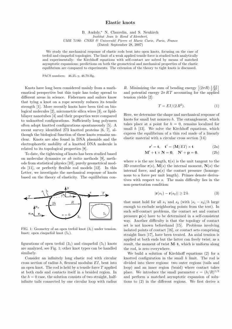
FIG. 1: Geometry of an open trefoil knot (31) under tension.Inset: open cinquefoil knot (51).

figurations of open trefoil (31) and cinquefoil (51) knotsare analyzed, see Fig. 1; other knot types can be handledsimilarly.

Consider an infinitely long elastic rod with circularcross section of radius h, flexural modulus EI, bent intoan open knot. The rod is held by a tensile force T appliedat both ends and contacts itself in a braided region. Inthe h = 0 case, the solution consists of two straight, half-infinite tails connected by one circular loop with radius

R. Minimizing the sum of bending energy[(2πR) 1

2EIR2

]and potential energy 2π R T accounting for the appliedtension yields [2]:

T = EI/(2R2). (1)

Here, we determine the shape and mechanical response ofknots for small but nonzero h. The entanglement, whichtakes place at a point for h = 0, remains localized forsmall h [13]. We solve the Kirchhoff equations, whichexpress the equilibrium of a thin rod made of a linearlyelastic material with a circular cross section [14]:

r′ = t, t′ = (M/EI) × t (2a)M′ + t × N = 0, N′ + p = 0. (2b)

where s is the arc length, t(s) is the unit tangent to the3D centerline r(s), M(s) the internal moment, N(s) theinternal force, and p(s) the contact pressure (homoge-nous to a force per unit length). Primes denote deriva-tives with respect to s. The main difficulty lies in thenon-penetration condition:

|r(s1) − r(s2)| ≥ 2h (3)

that must hold for all s1 and s2 (with |s1 − s2|/h largeenough to exclude neighboring points from the test). Insuch self-contact problems, the contact set and contactpressure p(s) have to be determined in a self-consistentway. Another difficulty is that the topology of contactset is not known beforehand [15]. Problems involvingisolated points of contact [16], or contact sets comprisingstraight lines [17], have been treated. An axial tension isapplied at both ends but the latter can freely twist; as aresult, the moment of twist M · t, which is uniform alongthe rod, is zero everywhere.

We build a solution of Kirchhoff equations (2) for aknotted configuration in the small h limit. The rod isdivided into three regions: two outer regions (tails andloop) and an inner region (braid) where contact takesplace. We introduce the small parameter ε = (h/R)1/2

and perform a matched asymptotic expansion of solu-tions to (2) in the different regions. We first derive a

2

scaling law for the length � of the braid, assuming � isan intermediate quantity, h � � � R. In the braid,of length �, transverse displacements are of order h: thecenterline has a slope of order h/� with respect to the zaxis. Points in the loop at a distance of order � from theaxis of symmetry y have a slope ∼ �/R. Equating thesetwo slopes requires � to be of order

√hR.

The rod configuration in the tails is found, to firstorder in ε, by solving equations (2) linearized near thestraight configuration (t = ez, M = 0 and N = T ez),where ex,y,z are unit vectors defined in Fig. 1. Thefirst order correction for the tails is found to have anexponential profile, proportional to e−|z|

√T/EI . Sim-

ilarly, the loop part is solved to first order by lin-earizing equations (2) near a circular configuration t =sin(s/R) ey − cos(s/R) ez, M = (EI/R)ex and N = 0,where −π R < s < π R. The perturbed loop configura-tion is found to remain planar, although in a plane thatis slightly tilted about the y axis. The details of thecalculations are omitted.

Let us proceed to the inner solution. The braid is thecrucial region where the external tensile load T in thetails is transformed, with the help of contact forces, intothe internal bending moment EI/R in the loop. Accord-ing to the previous scalings, the slope in the braid issmall, of order ε. Geometric nonlinearities can then beneglected and the leading order of system (2) for strand‘a’, with centerline ra = (xa, ya, za), reads: EIx′′′′

a = pxa ,

EIy′′′′a = py

a, z′a = 1 where pxa = |p| (xb − xa)/(2h) and

pya = |p| (yb − ya)/(2h) are the components of the con-

tact force, assuming that there is no friction. The equa-tions for the other strand ‘b’ are similar, with px

b = −pxa

and pyb = −py

a by the action-reaction principle. We takeadvantage of the linearity of these equations and sepa-rate the inner problem into an average and a differenceproblem. To this end, we introduce the new variables〈r(s)〉 = (ra(s) + rb(s))/2 and r = (rb(s) − ra(s))/2.

The average problem gives the position of the curvelying halfway in between the two strands. It obeys theKirchhoff linearized equations: EI〈x〉′′′′ = 0, EI〈y〉′′′′ =0, with the asymptotic conditions 〈x〉′′ = 1/(2R) at bothends to allow matching with the loop. Note that thecontact forces cancel out in the average problem. Asa result, it has an obvious solution, namely an arc ofcircle with radius 2R, up to a rigid-body rotation andtranslation.

The difference problem tells how the two strands con-tact and wind around each other. The components ofr satisfy the Kirchhoff linearized equations: EI x′′′′ =|p|x/h, EI y′′′′ = |p| y/h. Based on the previous scalinganalysis, we introduce the rescaled quantities:

u =xb − xa

2h, v =

yb − ya

2h, w =

z

(2hR)1/2. (4)

Since the tangent deviates only slightly from ez, the arclength s � z, or w in rescaled coordinates, can be used

-1-0.50.51

-0.5

0.5

1

2 4

-0.5

0.5

1

(a)

(b) (c)

Q

Q

u

v v

w

uvw u2 + v2 = 1

wc

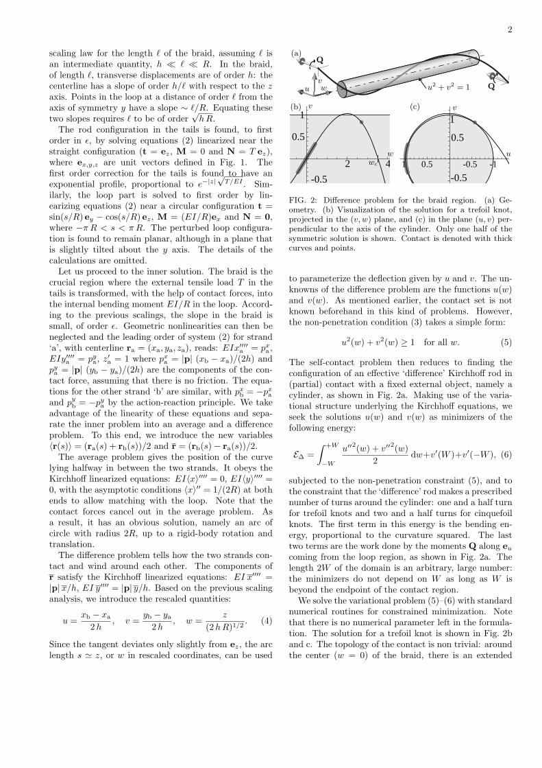
FIG. 2: Difference problem for the braid region. (a) Ge-ometry. (b) Visualization of the solution for a trefoil knot,projected in the (v, w) plane, and (c) in the plane (u, v) per-pendicular to the axis of the cylinder. Only one half of thesymmetric solution is shown. Contact is denoted with thickcurves and points.

to parameterize the deflection given by u and v. The un-knowns of the difference problem are the functions u(w)and v(w). As mentioned earlier, the contact set is notknown beforehand in this kind of problems. However,the non-penetration condition (3) takes a simple form:

u2(w) + v2(w) ≥ 1 for all w. (5)

The self-contact problem then reduces to finding theconfiguration of an effective ‘difference’ Kirchhoff rod in(partial) contact with a fixed external object, namely acylinder, as shown in Fig. 2a. Making use of the varia-tional structure underlying the Kirchhoff equations, weseek the solutions u(w) and v(w) as minimizers of thefollowing energy:

E∆ =∫ +W

−W

u′′2(w) + v′′2(w)2

dw+v′(W )+v′(−W ), (6)

subjected to the non-penetration constraint (5), and tothe constraint that the ‘difference’ rod makes a prescribednumber of turns around the cylinder: one and a half turnfor trefoil knots and two and a half turns for cinquefoilknots. The first term in this energy is the bending en-ergy, proportional to the curvature squared. The lasttwo terms are the work done by the moments Q along eu

coming from the loop region, as shown in Fig. 2a. Thelength 2W of the domain is an arbitrary, large number:the minimizers do not depend on W as long as W isbeyond the endpoint of the contact region.

We solve the variational problem (5)–(6) with standardnumerical routines for constrained minimization. Notethat there is no numerical parameter left in the formula-tion. The solution for a trefoil knot is shown in Fig. 2band c. The topology of the contact is non trivial: aroundthe center (w = 0) of the braid, there is an extended

3

�

R

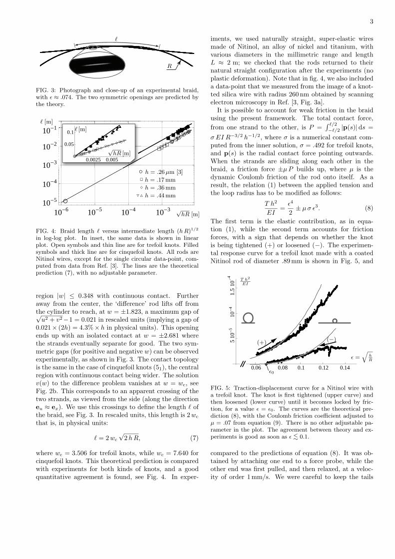
FIG. 3: Photograph and close-up of an experimental braid,with ε ≈ .074. The two symmetric openings are predicted bythe theory.

10 6 10 5 10 4 10 3 10 5

10 4

10 3

10 2

10 1

0.0025 0.005

0.05

0.1

√hR [m]

√hR [m]

� [m]

� [m]

h = .26 µm [3]

h = .17 mm

h = .36 mm

h = .44 mm

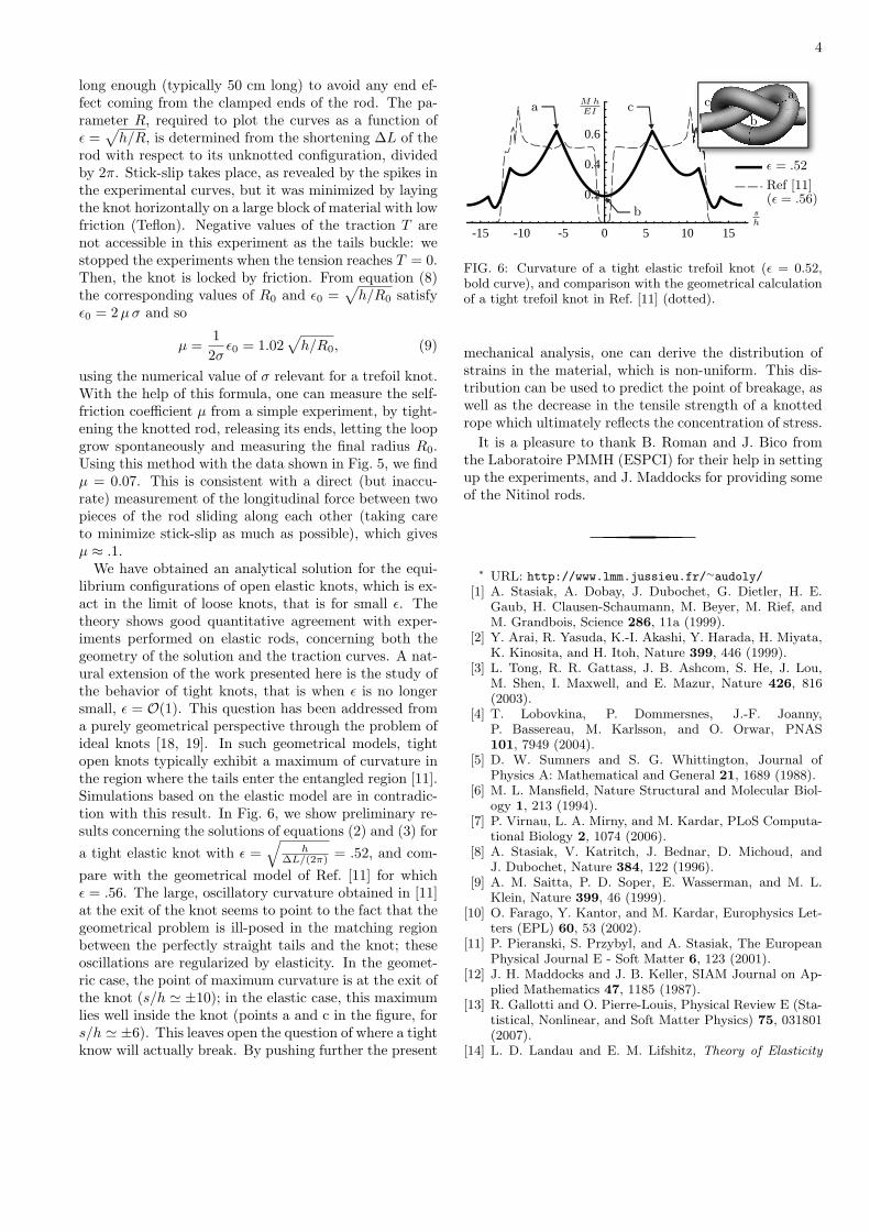
FIG. 4: Braid length � versus intermediate length (h R)1/2

in log-log plot. In inset, the same data is shown in linearplot. Open symbols and thin line are for trefoil knots. Filledsymbols and thick line are for cinquefoil knots. All rods areNitinol wires, except for the single circular data-point, com-puted from data from Ref. [3]. The lines are the theoreticalprediction (7), with no adjustable parameter.

region |w| ≤ 0.348 with continuous contact. Furtheraway from the center, the ‘difference’ rod lifts off fromthe cylinder to reach, at w = ±1.823, a maximum gap of√

u2 + v2−1 = 0.021 in rescaled units (implying a gap of0.021× (2h) = 4.3%×h in physical units). This openingends up with an isolated contact at w = ±2.681 wherethe strands eventually separate for good. The two sym-metric gaps (for positive and negative w) can be observedexperimentally, as shown in Fig. 3. The contact topologyis the same in the case of cinquefoil knots (51), the centralregion with continuous contact being wider. The solutionv(w) to the difference problem vanishes at w = wc, seeFig. 2b. This corresponds to an apparent crossing of thetwo strands, as viewed from the side (along the directioneu ≈ ex). We use this crossings to define the length � ofthe braid, see Fig. 3. In rescaled units, this length is 2wc

that is, in physical units:

� = 2wc

√2hR, (7)

where wc = 3.506 for trefoil knots, while wc = 7.640 forcinquefoil knots. This theoretical prediction is comparedwith experiments for both kinds of knots, and a goodquantitative agreement is found, see Fig. 4. In exper-

iments, we used naturally straight, super-elastic wiresmade of Nitinol, an alloy of nickel and titanium, withvarious diameters in the millimetric range and lengthL ≈ 2 m; we checked that the rods returned to theirnatural straight configuration after the experiments (noplastic deformation). Note that in fig. 4, we also includeda data-point that we measured from the image of a knot-ted silica wire with radius 260 nm obtained by scanningelectron microscopy in Ref. [3, Fig. 3a].

It is possible to account for weak friction in the braidusing the present framework. The total contact force,from one strand to the other, is P =

∫ �/2

−�/2|p(s)|ds =

σ EI R−3/2 h−1/2, where σ is a numerical constant com-puted from the inner solution, σ = .492 for trefoil knots,and p(s) is the radial contact force pointing outwards.When the strands are sliding along each other in thebraid, a friction force ±µP builds up, where µ is thedynamic Coulomb friction of the rod onto itself. As aresult, the relation (1) between the applied tension andthe loop radius has to be modified as follows:

T h2

EI=

ε4

2± µσ ε3. (8)

The first term is the elastic contribution, as in equa-tion (1), while the second term accounts for frictionforces, with a sign that depends on whether the knotis being tightened (+) or loosened (−). The experimen-tal response curve for a trefoil knot made with a coatedNitinol rod of diameter .89mm is shown in Fig. 5, and

0.06 0.08 0.1 0.12 0.14

510

510

410

1.5

4

ε =q

hR

ε0

T h2

EI

(+)(−)

FIG. 5: Traction-displacement curve for a Nitinol wire witha trefoil knot. The knot is first tightened (upper curve) andthen loosened (lower curve) until it becomes locked by fric-tion, for a value ε = ε0. The curves are the theoretical pre-diction (8), with the Coulomb friction coefficient adjusted toµ = .07 from equation (9). There is no other adjustable pa-rameter in the plot. The agreement between theory and ex-periments is good as soon as ε <∼ 0.1.

compared to the predictions of equation (8). It was ob-tained by attaching one end to a force probe, while theother end was first pulled, and then relaxed, at a veloc-ity of order 1mm/s. We were careful to keep the tails

4

long enough (typically 50 cm long) to avoid any end ef-fect coming from the clamped ends of the rod. The pa-rameter R, required to plot the curves as a function ofε =

√h/R, is determined from the shortening ∆L of the

rod with respect to its unknotted configuration, dividedby 2π. Stick-slip takes place, as revealed by the spikes inthe experimental curves, but it was minimized by layingthe knot horizontally on a large block of material with lowfriction (Teflon). Negative values of the traction T arenot accessible in this experiment as the tails buckle: westopped the experiments when the tension reaches T = 0.Then, the knot is locked by friction. From equation (8)the corresponding values of R0 and ε0 =

√h/R0 satisfy

ε0 = 2µσ and so

µ =12σ

ε0 = 1.02√

h/R0, (9)

using the numerical value of σ relevant for a trefoil knot.With the help of this formula, one can measure the self-friction coefficient µ from a simple experiment, by tight-ening the knotted rod, releasing its ends, letting the loopgrow spontaneously and measuring the final radius R0.Using this method with the data shown in Fig. 5, we findµ = 0.07. This is consistent with a direct (but inaccu-rate) measurement of the longitudinal force between twopieces of the rod sliding along each other (taking careto minimize stick-slip as much as possible), which givesµ ≈ .1.

We have obtained an analytical solution for the equi-librium configurations of open elastic knots, which is ex-act in the limit of loose knots, that is for small ε. Thetheory shows good quantitative agreement with exper-iments performed on elastic rods, concerning both thegeometry of the solution and the traction curves. A nat-ural extension of the work presented here is the study ofthe behavior of tight knots, that is when ε is no longersmall, ε = O(1). This question has been addressed froma purely geometrical perspective through the problem ofideal knots [18, 19]. In such geometrical models, tightopen knots typically exhibit a maximum of curvature inthe region where the tails enter the entangled region [11].Simulations based on the elastic model are in contradic-tion with this result. In Fig. 6, we show preliminary re-sults concerning the solutions of equations (2) and (3) fora tight elastic knot with ε =

√h

∆L/(2π) = .52, and com-

pare with the geometrical model of Ref. [11] for whichε = .56. The large, oscillatory curvature obtained in [11]at the exit of the knot seems to point to the fact that thegeometrical problem is ill-posed in the matching regionbetween the perfectly straight tails and the knot; theseoscillations are regularized by elasticity. In the geomet-ric case, the point of maximum curvature is at the exit ofthe knot (s/h � ±10); in the elastic case, this maximumlies well inside the knot (points a and c in the figure, fors/h � ±6). This leaves open the question of where a tightknow will actually break. By pushing further the present

0.2

0.4

0.6

-15 -10 -5 0 5 10 15

sh

M hEI

a

b

ca

b

c

ε = .52

Ref [11](ε = .56)

FIG. 6: Curvature of a tight elastic trefoil knot (ε = 0.52,bold curve), and comparison with the geometrical calculationof a tight trefoil knot in Ref. [11] (dotted).

mechanical analysis, one can derive the distribution ofstrains in the material, which is non-uniform. This dis-tribution can be used to predict the point of breakage, aswell as the decrease in the tensile strength of a knottedrope which ultimately reflects the concentration of stress.

It is a pleasure to thank B. Roman and J. Bico fromthe Laboratoire PMMH (ESPCI) for their help in settingup the experiments, and J. Maddocks for providing someof the Nitinol rods.

∗ URL: http://www.lmm.jussieu.fr/∼audoly/[1] A. Stasiak, A. Dobay, J. Dubochet, G. Dietler, H. E.

Gaub, H. Clausen-Schaumann, M. Beyer, M. Rief, andM. Grandbois, Science 286, 11a (1999).

[2] Y. Arai, R. Yasuda, K.-I. Akashi, Y. Harada, H. Miyata,K. Kinosita, and H. Itoh, Nature 399, 446 (1999).

[3] L. Tong, R. R. Gattass, J. B. Ashcom, S. He, J. Lou,M. Shen, I. Maxwell, and E. Mazur, Nature 426, 816(2003).

[4] T. Lobovkina, P. Dommersnes, J.-F. Joanny,P. Bassereau, M. Karlsson, and O. Orwar, PNAS101, 7949 (2004).

[5] D. W. Sumners and S. G. Whittington, Journal ofPhysics A: Mathematical and General 21, 1689 (1988).

[6] M. L. Mansfield, Nature Structural and Molecular Biol-ogy 1, 213 (1994).

[7] P. Virnau, L. A. Mirny, and M. Kardar, PLoS Computa-tional Biology 2, 1074 (2006).

[8] A. Stasiak, V. Katritch, J. Bednar, D. Michoud, andJ. Dubochet, Nature 384, 122 (1996).

[9] A. M. Saitta, P. D. Soper, E. Wasserman, and M. L.Klein, Nature 399, 46 (1999).

[10] O. Farago, Y. Kantor, and M. Kardar, Europhysics Let-ters (EPL) 60, 53 (2002).

[11] P. Pieranski, S. Przybyl, and A. Stasiak, The EuropeanPhysical Journal E - Soft Matter 6, 123 (2001).

[12] J. H. Maddocks and J. B. Keller, SIAM Journal on Ap-plied Mathematics 47, 1185 (1987).

[13] R. Gallotti and O. Pierre-Louis, Physical Review E (Sta-tistical, Nonlinear, and Soft Matter Physics) 75, 031801(2007).

[14] L. D. Landau and E. M. Lifshitz, Theory of Elasticity

5

(Course of Theoretical Physics) (Pergamon Press, 1981),2nd ed.

[15] H. von der Mosel, Annales de l’I. H. P., section C 16, 137(1999).

[16] G. H. M. van der Heijden, S. Neukirch, V. G. A. Goss,and J. M. T. Thompson, International Journal of Me-chanical Sciences 45, 161 (2003).

[17] B. Coleman and D. Swigon, Journal of Elasticity 60, 173(2000).

[18] A. Stasiak, V. Katritch, and L. H. Kauffman, eds., IdealKnots (World Scientific, Singapore, 1998).

[19] J. Baranska, P. Pieranski, S. Przybyl, and E. J. Rawdon,Phys. Rev. E 70, 051810 (2004).