UCRL-ID- 13 1770

Elastic Properties of Sand-Peat Moss Mixtures fro-m Ultrasonic Measurements

Cosette Trombino

September 2,1998

This is an informal report intended primarily for internal or limited external distribution. The opinions and conclusions stated are those of the author and may 01 may not be those of the Laboratory. Work performed under the auspices of the U.S. Department of Energy by the Lawrence Livermore National Laboratori under Contract W-7405.ENG-48.

DISCLAIMER

This document was prepared as an account of work sponsored by an agency of the United States Government. Neither the United States Government nor the University of California nor any of their employees, makes any warranty, express or implied, or assumes any legal liability or responsibility for the accuracy, completeness, or usefulness of any information, apparatius, product* or process disclosed, or represents that its use would not infringe privately owned rights. Reference herein to any specific commercial product, process, or service by trade name, trademark, manufacturer, or otherwise,~does not necessarily constitute or imply its endorsement, recommendation, or favoring by the United States Government or the University of California. The views and opinions of authors expressed herein do not necessarily state or reflect those of the United States Government or the University of California, and shall not be used for advertising or product endorsement purposes.

This report has been reproduced directly from the best available copy,

Available to DOE and DOE contractors from the Office of Scientific and Technical Information

P.O. Box 62, Oak Ridge, TN 37831 Prices available from (423) 576-8401

Available to the public from the National Technical Information Service

U.S. Department of commerce 5285 Port Royal Rd.,

Springfield, VA 22161

Elastic Properties of Sand-Peat Moss Mixtures from Ultrasonic Measurements

Cosetie Trombino

Abstract

Effective remediation of an environmental site requires extensive knowledge of the geologic setting, as well as the amount and distribution of contaminants. Seismic investigations provide a means to examine the subsurface with minimum disturbance, Laboratory measurements are needed to interpret field data.

In this experiment, laboratory tests were performed to characterize manufactured soil samples in terms of their elastic properties. The soil samples consisted of small (mass) percentages (1 to 20 percent) of peat moss mixed with pure quartz sand. Sand was chosen as the major component because its elastic properties are well known except at the lowest pressures. The ultrasonic pulse transmission technique was used to collect elastic wave velocity data. These data were analyzed and mathematically processed to calculate the other elastic properties such as the modulus of elasticity.

This experiment demonstrates that seismic data are affected by the amount~of peat moss added to pure sand samples. Elastic wave velocities, velocity gradients, and elastic moduli vary with pressure and peat moss amounts. In particular, ultrasonic response changes dramatically when pore space fills with peat. With some further investigation, the information gathered in this experiment could be applied to seismic field research.

r

l Background

Site characterization is an important step towards in-situ remediation. Several methods have been used to examine the physical properties of soil in the near subsurface. One important method is seismic interrogation, which involves measuring the velocities of elastic waves that travel through the subsurface. Effective seismic interrogation requires that measured parameters be related to soil properties. Laboratory experiments that measure elastic wave velocities in manufactured soils can provide tield researchers with methods for interpreting field-collected data.

Since the elastic properties of pure quark sand are well known (Domenico, 1976) except at the lowest pressures, pure quartz sand is often used to make reference measurements. The microstructure of the sample is altered with controlled “impurities” such as clay (or as in this experiment, peat moss), and ultrasonic measurements are made in the laboratory to characterize the associated effects.

In laboratory samples, it has been found that small amounts of swelling clay dramatically change the way seismic energy propagates through unconsolidated soils (Bonner et al., 1997). Seismic field data are therefore disproportionately affected by the presence of swelling clay. Clay blocks fluid flow, and to a large degree controls how fluids circulate as contaminants spread or are removed by remediation.

Soil composition (i.e., clay content) is only one factor that influences contaminant transport in the near subsurface. Other parameters such as porosity, permeability, and fluid saturation are important to site characterization. Electrical methods have been used to quantify these parameters, and studies (Harris et al., 1995, Berge et al., 1998) suggest that these methods could

be combined with seismic information about compressional and shear velocities to image the shallow subsurface.

l Motivation

Lawrence Livermore National Laboratory has been involved in the effort to find a cost-effective alternative to current methods of contaminated site characterization. Geophysical techniques (including seismic, electrical, and magnetic methods) can be used to image the earth’s shallow subsurface. These methods of imaging are much cheaper and less invasive than drilling many monitoring wells. Geophysical imaging techniques also have the potential to be more accurate and complete than traditional methods in predicting contaminant amounts and distributions, because geophysical methods provide three-dimensional information rather than providing data from one point in space at one instant in time.

A geophysical image shows the variation in physical properties for a particular volume or area element. A seismic image shows how elastic wave velocity varies with position. Therefore, an image is a measured attribute of the material, and calibration is necessary for accurate image interpretation. One way to calibrate the image is to perform laboratory measurements of the attributes (i.e., elastic wave velocity) for known standard materials. This paper provides an analysis of data gathered in such a calibration experiment using sand and peat moss (in prescribed combinations) as standards. The aim of the experiment is to develop a model by which to interpret field data.

Ultimately, geophysical imaging could result in faster and more effective in-situ remediation of contaminated sites. In addition, geophysical imaging has applications in civil engineering (e.g., locating clay layers that limit slope stability). Geophysical images might also assist prediction of ground motion during seismic activity by locating soils prone to liquifaction.

l Previous Work

Many studies have been done on the elastic properties of unconsolidated materials such as sand and soil (e.g., Wyllie et al., 1958; Whitman, 1966; Banner et al., 1997). Several examples exist in the geotechnical, civil engineering, geophysics, and marine acoustics literature (e.g., Domenico, 1976; Hamilton and Bachman, 1982). Such studies involve measuring elastic moduli or elastic wave velocities in unconsolidated materials (e.g., Hughes and Jones, 1950). The work described in this report uses standard ultrasonic methods (Trimmer et al., 1980) to measure elastic velocities at ultrasonic frequencies. This work builds on previous work conducted at Lawrence Livermore National Laboratory (Banner et al., 1997). Compressional and shear velocities have been determined experimentally for pure Ottawa sand samples confined hydrostatically. In the work described here, the effects of peat moss on acoustic and mechanical properties of the near subsurface were investigated to expand on similar studies involving mixtures of clay and sand.

. Theoretical Background

The two types of elastic waves that are important to seismic investigation are the compressional, or primary (P) waves and the shear, or secondary (S) waves (Aki and Richards, 1980). Both of these waves fall under the category of body waves, or waves that travel through the interior of a rock body. P-waves travel in any direction where compression is opposed, inducing longitudinal oscillatory particle motions similar to simple harmonic vibrations. S-waves are byproducts of P-

waves, occurring when P-waves impinge on a free boundary indirectly and cause displacement. S-waves only travel in material that resists changes in shape, so they do not travel in fluids.

Elastic waves with seismic frequencies (about 1 Hz to 100 kHz) are called seismic waves. Sound waves are P-waves at frequencies that the human ear can detect (about 20 Hz to 20 kHz). Elastic waves with high frequencies (about 20 kHz to 100 MHZ) are called ultrasonic waves.

Both P- and S- wave velocities can be determined theoretically by applying basic physics concepts to a differential area. The sum of the forces on a differential area is equal to the product of its mass and acceleration.

If the area element is not a solid, there can be no acoustic shear forces acting upon it, For example, in the one-dimensional case, compressional and shear waves obey the wave equation (Young and Freedman, 1996):

S2y(x,t) 1 S2y(x,t) 6x2 =7 &P

(Eq.1)

where y(x,t) is the wave function x = position t = time, and v = velocity (compressional or shear wave).

The velocity of the propagating wave is determined by the elastic properties of the medium, as given in the following equations (Lama and Vutukuri, 1978):

VP= E(l-v) $

p(l+ v)(l-2v) = 1 vs=[;]'=[2A'i+")]:

4 ’ K+-G T 3 [ 1 P

(Eq.2)

(Eq.3)

where . VP = velocity of compressional waves, m/s or in/s vs = velocity of shear waves, m/s or ht/s E = dynamic modulus of elasticity (Young’s modulus), Pa or lbUin2 K = dynamic bulk modulus (inverse of compressibility), Pa or lbf/in’ G = dynamic modulus of rigidity, Pa or Ibf7in2 v = Poisson’s ratio, and p = density, kg/m3 or lb&n’.

In this laboratory experiment, ultrasonic wave velocities for P- and S- waves were determined from measured wave arrival times and the known lengths of the samples:

“- 1cJ’z L-t,

where v.= velocity (of compressional or shear waves), m/s 1 O4 = factor converting cm+ to m/s [= distance traveled by wave, measured to be 1.770 +0.005 in (4.496 f0.013 cm), and &-to = travel time of wave (b established by aluminum calibration experiments), ps.

The aluminum calibration experiments involved substituting pure aluminum samples for the regular samples to determine the total lag time introduced by cables and connections in the sample setup. The aluminum samples were different length sections cut from a single aluminum bar. The arrival times were measured (see Experimental Setup and Procedure section) and plotted against length. The y-intercept given by a linear fit is the time ~adjustment. The compressional time adjustment (tm) was determined to be 1 ps, and the shear time adjustment (ba) was 3 PS.

Every experimental sample was made of three layers, each with a thickness of approximately l/3 the length of the sample (see Sample Preparation section). The total volume of the sample was measured by filling an empty sample assembly with deionized water, extracting the water with a syringe, then measuring the volume of the water in a graduated cylinder (knowing that 1 mL = 1 cm’). The density of the pure sand sample was determined mathematically to be 1691.92 kg/m’ from the volume of the cylinder, 78.0 cm3 -f 5%, the mass of sand that tills that volume, 13 1.97 g (all masses were measured by a Sartorius Analytic mass balance), and the equation relating the two:

where 1000 is the factor converting p to kg/ma, m = mass, g, and V = volume, cm’.

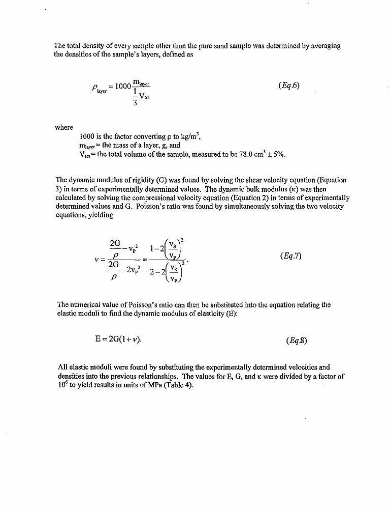
The total density of every sample other than the pure sand sample was determined by averaging the densities of the sample’s layers, defined as

(Eq.6)

where 1000 is the factor converting p to kg/m’, mraycr = the mass of a layer, g, and VtOt= the total volume of the sample, measured to be 78.0 cm3 f. 5%.

The dynamic modulus of rigidity (G) was found by solving the shear velocity equation (Equation 3) in terms of experimentally determined values. The dynamic bulk modulus (K) was then calculated by solving the compressional velocity equation (Equation 2) in terms of experimentally determined values and G. Poisson’s ratio was found by simultaneously solving the two velocity equations, yielding

C-Q.7

The numerical value of Poisson’s ratio can then be substituted into the equation relating the elastic moduli to find the dynamic modulus of elasticity (E):

E=2G(l+v). U-%.8)

All elastic moduli were found by substituting the experimentally determined velocities and densities into the previous relationships. ‘The values for E, G, and K were divided by a factor of IO6 to yield results in units of MPa (Table 4).

Laboratory Experiments

. Experimental Setup and Procedure

The experimental setup (Fig. 1) and flow (Fig. 2) were based on the method of ultrasonic pulse transmission (Sears and Banner, 1981).

r

Each sample is a packed mix of dry (room-temperature humidity) Ottawa sand and peat moss in a plastic shell designed to ensure that the signal is transferred through the soil mixture, rather than the shell.. The shell is capped with latex held in place by rubber O-rings. Latex was chosen to contain the soil mixture because it elastically deforms with the soil when pressure is applied and it has a minimal impact on the signal transmission.

For each measurement, a sample is placed between two heavily damped 500 kHz shear transducers (made by Panametrics) for elastic wave measurements, and is locked in place by adjusting the separation between the transducers to a minimum. The transducers produce sufficient compressional energy to identify bofh P- and S-wave arrivals. End-load pressures between 0 and 15 psi (0 to 0.11 MPa), simulating up to several meters of overburden, are applied to the sample through air-driven, pneumatic pistons (manufactured by Bimba) that push on the backs of fhe transducers. Although some small pressure (estimated to be less than 1 psi) is applied in the locking process, this is necessary for coupling, and any associated error in pressure readings is minimized by having one technician perform all the experiments and is not significant to calculations.

The end-load pressures are slowly applied in increments of 5 gauge units (or 1.56 psi) up to 50 gauge units (15.6 psi), then dropped in increments of 10 gauge units (3.12 psi), inducing static internal stress throughout the loading and unloading of the sample. To ensure consistent loading, house air (at 100 psi) is sent through a miniature compressed air filter (made by C. A. Norgren Co.) and a (Coilhouse Pneumatics) miniature regulator before it reaches the pneumatic pistons. The regulating knob controls the pressure that is sent to the pistons, and the regulator readout is the gauge pressure recorded.

A pulse generator (Fig. 3) sends 500 positive volts to activate the transmitting piezoelectric transducer (Transducer #l). The resultant ultrasonic wave produced by Transducer #l travels through the sample to the receiving transducer (Transducer #2). This ultrasonic wave is the dynamic stress that is used to image the sample. Transducer #2 converts the ultrasonic wave into electrical form, and the final signal is sent through a 40 to 60db signal preamplifier (a Panametrics preamp with a band pass of 20 kHz to 2 MHz) to a LeCroy 9400 Dual 125 MHz digital oscilloscope (Oscilloscope #l). Oscilloscope #l plots the excitation signal sent to Transducer #l (Channel 1) and the signal received by Transducer #2 (Channel 2) as functions of time. The pulse generator provides timing synchronization to both oscilloscopes. The Channel 1 display establishes the signal starting time. The Channel 2 information is simultaneously sent to a LeCroy 9430 10 bit 150 MHz digital oscilloscope (Oscilloscope #2). Oscilloscope #I and Oscilloscope #2 produce identical functions of the Channel 2 data by averaging 1000 sequential repetitive signals to improve the signal-to-noise ratio.

After the pre-amp and oscilloscope settings are adjusted to prevent clipping, the arrival times of the compressional (P) and shear(S) waves are determined through observation of the Channel 2 display (Fig. 4a-f) and recorded (Table 1). Human judgement was used to pick the arrival times in this experiment (see Results section), and we are currently automating the process to minimize

error. Oscilloscope I#2 digitizes the collected data and sends them to an attached Macintosh computer (MAC #l) through a transfer program written using National Instruments LabView software. MAC #l is networked to another Macintosh computer (MAC #2), where the data are stored for data reduction and signal processing using the Synergy Software program KaleidaGraph. A LabView program (currently being written) will filter the data, determine the frequency content, and automate the arrival time selection.

l Sample Preparation

Earlier experiments involved flushing sand-clay samples with solutions during data collection. To ensure even distribution of the solution (and to prevent clay clogging of fluid inlet ports), a middle layer of sand was included in every sample. Although the samples examined in this paper were unsaturated, each one included a central sand layer for consistency. The other two layers were sand-peat mixtures (the same for each layer).

Every sample used pure quartz (Gttowa) sand. This sand comes from a quarry near the city of Ottawa, Illinois and is Middle Ordovician in age. The sand is composed entirely of quartz grains (Domenico, 1976). The grain sizes of the tested sand are between 74 and 420 pm, and the median grain diameter is 273 pm (Aracne-Ruddle et al., 1998).

All peat mixtures used 100% Canadian Sphagnum peat moss with an added polyoxakylene glycol (8 ppm) wetting agent. This peat moss is readily available from garden and nursery suppliers. We did not perform chemical analyses to determine the composition of the peat. Peat is a soil with a very high percentage of organic matter and very low percentage of mineral components. Typical organic content of peat moss is 80 to 95% of the mass fraction. Since the samples were not water saturated in these experiments, the mechanical properties are assumed to be unaffected by the wetting agent that was added by the peat moss supplier.

The sand-peat mixtures used in each sample are combined and weighed separately, and the weight percentages are calculated precisely. This experiment used samples with sand-peat layer weight ratios of 99: 1,97:3,90:10, and SO:20 in addition to the (control) 100% sand sample (Table 2).

Every sample was prepared following the same procedure. First, the sample assembly (acrylic shell, latex caps, and rubber o-rings) is weighed empty. After the sample assembly mass has been recorded (Table 2), the assembly is filled to approximately l/3 of its volume by a portion of the sand/peat mixture. The sand-peat mixture is packed by a hand-held brass weight that fits snugly inside the acrylic shell (Fig. 5). The combination of assembly and sand/peat mixture is weighed, and the mass is recorded. Next, the assembly is tilled to approximately 2/3 of its capacity by adding a layer of pure sand, and the contents of the assembly are packed again. The assembly and its contents are reweighed, and the mass is recorded. Finally, the assembly is tilled to capacity with a second layer of the sand/peat mixture, packed, and weighed. The final weight is recorded. The true masses of the assembly and each layer of material are used to calculate approximate layer and total densities with Equation 6 and Equation 7 (Table 2).

Results

The results of ultrasonic velocity calculations are shown in Table 3. The elastic moduli are tabulated in Table 4.

The P-wave arrivals were picked at the first peaks evident in the signal (Fig 4a-f). The first trough was also identified. Error bars were assigned to every pick (Table 1). The first peak (“a” in most cases, “b” in the 20% peat moss sample) arrival times were used for velocity calculations (Table 3). Peaks were used rather than zero crossings for consistency.

The S-wave arrivals were more difficult to pinpoint. Several points were identified on the waveform and assigned uncertainties. These points were typically chosen to coincide with the first peak and the first trough before a major amplitude increase and accompanying frequency change indicative of second (shear) phase interference with the original (compressional) phase. After all the measurements were taken, plots of the oscilloscope displays were compared, and the points at the first troughs before the amplitude increases were chosen as the most consistent indicators of the shear arrivals. The points with the following labels were used for shear velocity calculations: 0% - b, 1% - c, 3% - b, 10% - a, 20% - a for 6.24 and 7.8 psi, c for 9.36 psi on, where the % indicates the percentage of peat moss in the respective samples’ peat-sand layers.

l Ultrasonic velocities

l Individual Samples

The compressional (P) and shear(S) wave velocities calculated in Table 3 were plotted as functions of loading stresses for each sample.

The pure sand sample (Fig. 6a) has P-wave velocities between 200 and 400 m/s and S-wave velocities between 100 and 250 m/s. These velocities are typical for unconsolidated materials, but are an order of magnitude lower than velocities in rocks. Both P- and S-wave velocities increase with added end-load pressure (stress) in the pure sand sample. Hysteresis is more noticeable for the P-wave velocities than for the S-wave velocities, but is not significant in either. Both the shear and compressional velocity gradients are steep at low stresses. At higher stresses, the shear velocity gradient flattens more significantly than the compressional velocity gradient.

The compressional and shear velocities in the 1% peat moss sample (Fig. 6b) are lower than the velocities of the pure sand sample. At the lowest stresses, the attenuation was so high that shear arrival times couldn’t be picked and compressional arrival time picks were scattered (Table 1). The shear velocity gradient seems to flatten with increased stress as it did in the pure sand sample, and is flatter than the compressional velocity gradient at high stresses. Greater hysteresis is evident in both velocities, but the effect is still smaller than the scatter of data points.

The compressional and shear velocities in the 3% peat moss sample (Fig. 6~) are approximately the same as those of the 1% peat moss sample. However, the maximum compressional velocity is higher for the 3% peat moss sample than for the 1%. There is less scatter and attenuation in the plots, and the characters of the slopes are different. One compressional velocity data point (3.12 psi, 468.30 m/s) was omitted from the plot, because the data for that point were collected after the sample was unlocked and relocked, producing a different waveform. The compressional and shear velocity gradients are initially flat. As stress is increased, the gradients increase. At the

highest stresses, the compressional velocity gradient remains steep but the shear velocity gradient flattens.

The compressional and shear velocities in the 10% peat moss sample (Fig. 6d) are considerably faster than the velocities of the pure sand, l%, and 3% samples (especially at low stresses). The velocity gradients are flatter for both wave types, and appear to be concave down at low stresses. Large uncertainties in shear wave arrival times (Table 1) due to the unique shape of the waveform (Fig. 4~) affect the shear velocity plot.

The 20% peat moss sample demonstrates extremely low shear velocities and velocity gradient but an extremely high compressional velocity gradient. This sample showed large hysteresis at pressures above 9 psi. High uncertainties are associated with both the compressional and the shear wave arrival times (Table 1), and thus the velocity plots.

l Graphical Velocity Comparison

Figure 7 compares the compressional velocities of all samples but the 20% peat moss sample (which was omitted due to its high uncertainties and scatter). Figure 8 compares the shear velocities of all the samples.

In Figure 7, the pure sand compressional velocity data points are fitted to a line to highlight the pure sand behavior. The compressional sand~velocities follow an approximately linear trend. The 10% peat moss sample has higher velocities than the pure sand sample, and all the other samples have velocities lower than the pure sand sample. For the 1,3, and 10% peat moss samples, compressional wave velocity increases systematically with peat moss addition. There is no systematic change in slope with sample composition.

In Figure 8, there are no clear patterns. With the exception of the 10% sample, the shear velocities in the sand-peat mixtures are lower at all stresses than the corresponding velocities in the pure sand. The 20% peat sample has the lowest velocities, and the 10% peat sample has the highest velocities. There is no systematic increase in velocity with added peat moss. There is no systematic change in slope with sample composition. Although the pure sand shear velocity data points are fitted to a line, they do not appear to follow a linear pattern (the velocity gradient is steep for low stresses and flat for high stresses).

l Velocity Ratios (VpIVs)

The range of values for the velocity ratio VpNs is 1.25 to 3.44. These extreme values are both from the 20% peat sample (which has high uncertainties associated with the velocities). The ranges of velocity ratios for the other samples are as follows: 1% - 1.56 to 1.80,3% - 1.63 to 1.94, 10% - 1.21 to 1.30, and pure sand - 1.66 to 1.92. The velocity ratio for the 1% peat sample decreases with increasing stress. The velocity ratio for the 3% peat sample increases with increasing stress. The velocity ratio for the 10% peat sample does not change systematically with stress. The velocity ratio for the 20% peat sample increases with increasing stress. The velocity ratio for the pure sand sample decreases with increasing stress. For consolidated sedimentary rocks, the Vdvs ratio is typically 1.5 to 2.0, with sandstones representing the lower values and calcareous rocks representing the higher values (Wilkens et al., 1984). Even though the elastic wave velocities of the samples are an order of magnitude smaller than velocities typical in consolidated, sedimentary rocks, the velocity ratios are similar.

l Elastic Moduli

l Poisson’s Ratio (v)

The ranges of Poisson’s ratio for the samples are as follows: I%, 0.15 to 0.28; 3%, 0.20 to 0.32; lo%, -0.55 to -0.22; 20%, -0.37 to 0.45; and pure sand, 0.21 to 0.31. The theoretical lim its on Poisson’s ratio for elastic materials are -1.00 to 0.500. The samples with the negative values for Poisson’s ratio are those with high P- and S-wave velocities, low velocity gradients, and anomalous waveform character.

. Shear Modulus (G)

The ranges (in MPa) of shear moduli for the samples are as follows: 1% - 27 to 50,3% - 28 to 53, 10% - 84 to 110,20% - 8.4 to 17, and pure sand - 27 to 8 1. The highest and lowest values are for the samples with negative Poisson’s ratios. These values are about two to three orders of magnitude lower than shear moduli values typically found for consolidated sedimentary rocks (e.g., W ikens et al., 1994).

. Elastic (Young’s) Modulus (E)

The ranges (in MPa) of elastic (Young’s) moduli for the samples are as follows: 1% - 67 to 110, 3% - 70 to 140,10% - 95 to 160,20% - 10 to 50, and pure sand - 69 to 200. The lowest values are for the sample with the highest percentage of peat moss and the highest uncertainty associated with the elastic wave arrival times. The highest values are for the sample with anomalous waveform character. These values are about two to three orders of magnitude lower than Young’s moduli values typically found for consolidated sedimentary rocks (e.g., W ikens et al., 1994).

. Bulk Modulus (K)

The ranges (in h4Pa) of bulk moduli for the samples are as follows: 1% - 42 to 69,3% - 40 to 130, 10% - 15 to 38,20% - 2.0 to 170, and pure sand- 52 to 130. The highest and lowest values are for the sample with the highest percentage of peat moss and the highest uncertainty associated with the elastic wave arrival times. These values are about two to three orders of magnitude lower than bulk moduli values typically found for consolidated sedimentary rocks (e.g., W ikens et al., 1994).

Discussion I Conclusions

Elastic wave velocity behavior is controlled by microstructure. The amount of peat moss, sand, Andy air in each sample, as well as the arrangement of these components, affects the P to S velocity ratio and velocity gradients.

The elastic wave behavior of the peat-sand samples is complicated. Some samples have velocities faster than pure sand, and some have velocities slower than pure sand. Some samples have steeper velocity gradients than pure sand, and some have shallower gradients than pure sand. These differences are not systematic.

The 1% peat moss sample follows the expected trend in which the compressional and shear velocities are lower than those of pure sand and the velocity gradients are approximately the same as for pure sand. This is expected because we have replaced a small amount of sand with a small amount of (slower) peat moss without significantly changing the microstructure.

The 3% peat moss sample is faster than the 1% peat moss sample, but not as fast as the pure sand sample. The compressional velocity gradient is steeper than that of the 1% peat sample, and the shear velocity gradient is approximately the same. This may be because the microstructure was changed when peat moss filled some pores (replacing some air). The change in microstructure has a greater effect on the compressional velocity than the shear velocity because peat moss does not have a cementing effect for the sample. Another factor affecting the velocities might be pre- compression of the peat within the sample. As the sample is built with latex caps parallel to the ground, mass is added to the top, and this has the effect of pre-compressing the bottom. This is not expected to be significant, because the total vertical stress created by building the sample vertically (the “lithostatic” stress equal to the sample height multiplied by sample density and gravitational acceleration) was less than 0.1 psi. Some permanent strain might have occurred as the peat-sand mixture was packed into the sample holder (indicated by the flat compressional velocity gradient for stresses below 4 psi). However, none of the pre-compression effects were significant for stresses above 4 psi for this sample. Another factor that may have influenced the compressional velocities is the moisture content of the peat moss. As more peat is added to a sample, the moisture content of the sample is increased (replacing some air with water). This affects the compressional velocities but not the shear velocities because the shear modulus of air is the same as the shear modulus for water (zero).

The 10% peat moss sample is much faster than any other samples, and has compressional and shear velocity gradients flatter than those of any other sample. The high velocities may be the result of peat moss tilling pore spaces (replacing air). The amount of air present in a sample is inversely proportional to the density of that sample. Figure 9 shows the density changes that occur as more peat is added to the sample mixture. The changing slope in Figure 9 demonstrates that a significant amount of air is replaced with peat when the mass percentage of peat changes from 3 to 10. Since the velocities of the 10% peat moss sample do not increase until stresses greater than 4 psi are applied, pm-compression may be a factor affecting velocity for low stresses. The slopes of the compressional and shear velocity curves for the 10% sample decrease with increasing stress (especially at the highest stresses). This behavior suggests that the peat moss, which now tills most of the spaces between the sand grains, increases in stiffness over this pressure range.

The 20% peat moss sample is much slower than any other samples, and has a shear velocity gradient approximately the same as for the other samples (excluding the 10% sample). Compressional velocity information for this sample is not reliable because the signal was weak.

This attenuation may be caused by having too few sand grains to form a continuous framework to transmit the ultrasonic waves. The relatively low shear velocities and high shear wave amplitudes are not understood and are currently under investigation.

The attenuation of the signals in the 30% peat moss sample was so large for both compressional and shear waves that arrivals could not be identified and velocities could not be determined. The waveforms were saved for this sample, and future work with signal processing may enable arrival identification.

Suggestions for Future Work

Many aspects of the experiment described in this report could have been more thoroughly investigated if time had permitted. Related future experiments would benefit from the following adjustments:

1. To ensure that densities are uniform, measure layer heights more accurately. 2. Perform hydrostatic tests on materials with the same compositions to see within what error

end-load pressures simulate shallow burial. 3. Control the moisture content of samples by controlling humidity (i.e., prepare samples in a

glove bag). 4. Try saturating samples in different solutions and measuring the differences in elastic wave

velocities. 5. Measure sample permeabilities and porosities to establish a relationship between elastic

properties and permeability. 6. Investigate (possibly using X-my methods) whether the elastic properties indicate whether or

not the pores are entirely tilled with peat. 7. Investigate the effects of higher end-load pressures. 8. Improve identification of arrivals through signal processing of waveforms.

Summary

Information about subsurface soil properties has many applications. One non-intrusive way to obtain this information is seismic interrogation. This method involves measuring the velocities of elastic waves that travel through the subsurface. Seismic velocity reveals information about physical structure and, combined with density information, enables derivation of material properties. Relationships between measured parameters and soil properties must be established if seismic interrogation is to be successful. Laboratory experiments can use controlled soils to establish such relationships. The experimental results can then be applied to field measurements.

The experiment described in this report used a modified ultrasonic technique to collect elastic wave velocity data from manufactured mixtures of peat moss and sand. The sand-peat moss mixtures were weighed and measured precisely for composition and density, then packed inside specially designed containers for testing. Each sample was locked in place between two heavily damped 500 kHz shear transducers as end-load pressures between 0 and 15 psi (0 to 0.11 MPa) were applied to the backs of the transducers by pneumatic pistons. A pulse generator began each test by providing timing synchronization to two oscilloscopes and supplying a voltage pulse through a preamplifier to the transmitting transducer. The oscilloscopes plotted the voltages received by the receiving transducer at each end-load stress as functions of time. These plots

were used to pick elastic wave arrival times. The arrival times were used to calculate the elastic wave velocities, which were in mm used to calculate elastic moduli.

The amounts and arrangement of peat moss, sand, and air in each sample (the microstructure of the sample) had a profound effect on the elastic wave velocity behaviors. The end-load pressures (simulated depth) also had a strong influence on velocity magnitudes and gradients. Secondary influences included pore tilling, pre-compression of sample mixtures, and sample moisture content. A particularly significant result was that the ultrasonic response changed dramatically when the density indicated that the pore space was filled with peat.

Acknowledgements

Pat Berge and Brian Banner were invaluable mentors. They provided constant assistance, instruction, and encouragement. They were generous with their time, geophysical knowledge, editing skills, and support.

Chantel Aracne-Ruddle was amazingly welcoming and helpful. She provided technical guidance throughout the experimental process.

Ed Hardy performed the aluminum calibrations and introduced me to the experimental method used in this report’s investigation.

Eric Carlberg, Jeff Roberta, and Dorthe Wildenschild introduced me to different aspects of the Joint Inversion of Geophysical Data project during my initial working weeks (when it seemed that everyone involved with the seismic element of the project was on vacation). Their input brought the larger goals of the project into perspective.

Bob Langland and the LLNL Mechanical Engineering Dept. graciously gave me the freedom to work on this project.

Wilbert Lick provided long-distance advising from UC Santa Barbara.

Ronna Nagel provided excellent administrative assistance.

Dave Trombino provided helpful information, motivation, and transportation.

Carl Boro provided technical support and banter.

I was proud and grateful to work with everyone involved with this project.

This work was performed under the auspices of the U. S. Department of Energy by the Lawrence Livermore National Laboratory under contract No. W-7405-ENG-48 and supported specifically by the DOE Office of Energy Research within the Offtce of Basic Energy Sciences, Division of Engineering and Geosciences. This project is funded as part of the Environmental Management Science Program (EMSP), a pilot program managed jointly by the Office of Energy Research and the Offtce of Environmental Management.

References

Aki, Keiiti, and Paul G. Richards, 1980, Quantitative Seismology: Theory and Methods, Volume I, W.H. Freeman and Co., New York.

Aracne-Ruddle, C., D. Wildenschild, B. Banner, and P. Berge, 1998, Direct observations of the morphology of sand-clay mixtures with implications for mechanical properties (abstract): submitted for presentation at the American Geophysical Union Annual Fall Meeting, to be held Dec. 6;,10, 1998, in San Francisco, CA.

Berge, P.A., J.G. Berryman, J.J. Roberts, and D. Wildenschild, 1998, Joint inversion of geophysical data for site characterization and restoration monitoring, EMSP project summary/progress report for FY98 for EMSP project 55411: Lawrence Livermore National Laboratory report UCRL-JC-128343, presented at the DOE Environmental Management Science Workshop held July 27-July 30, 1998, Chicago, IL, sponsored by the DOE EMSP and the American Chemical Society.

Banner, B.P., D.J. Hart, P.A. Berge, and C.M. Aracne, 1997, Influence of chemistry on physical properties: Ultrasonic velocities in mixtures of sand and swelling clay (abstract): Lawrence Livermore National Laboratory report UCRLJC-128306abs, Eos, Transactions of the American Geophysical Union 78 Fall Meeting Supplement, F679.

Domenico, S. N., 1976, Effect of brine-gas mixture on velocity in an unconsolidated sand reservoir: Geophysics 41,882-894.

Hamilton, Edwin L., and Richard T. Bachman, 1982, Sound velocity and related properties of marine sediments: J. Acoust. Sot. Am. 72 (6), 1891-1904.

Harris, J. M., R. C. Nolen-Hoeksema, R. T. Langan, M. Van Schaack, S. K. Lamratos, and J. W. Rector III, 1995, High-resolution crosswell imaging of a west Texas carbonate reservoir: Part l-- Project summary and interpretation: Geophysics 60,667--681.

Hughes, D. S., and Jones, H. J., 1950, Variation of elastic moduli of igneous rocks with pressure and temperature: Bull., Geol. Sot. Am. 61, 843-856.

Lama, R. D., and V. S. Vutukuri, 1978, Handbook on Mechanical Properties of Rocks: Testing Techniques and Results, Volume II, Trans Tech Publications, Clausthal, Germany, 195-196.

Sears, F. M., and Bonner, B. P., 1981, Ultrasonic attenuation measurement by spectral ratios utilizing signal processing techniques: IEEE Trans. On Geoscience and Remote Sensing GE19, 95-99.

Trimmer, D., B. Banner, H. C. Heard, and A. Duba, 1980, Effect of pressure and stress on water transport in intact and fractured gabbro and granite: J. Geophys. Res. 85,7059-7071.

Whitman, Robert V., 1966, The response of soils to dynamic loadings, report no. 25: miscellaneous studies of the formation of wave fronts in sand, MIT Dept. of Civil Engineering Research Report R66-32, Soils Pub. No. 196, MIT, Cambridge, Massachusetts.

Wilkens, Roy, Gene Simmons, and Lou Caruso, 1984, The ratio VpNs aa a discriminant of composition for siliceous limestones: Geophysics 49, 1850-1860.

Wyllie, M. R. J., A. R. Gregory, and G. H. F. Gardner, 1958, An experimental investigation of factors affecting elastic wave velocities in porous media: Geophysics 23,459493.

Young, Hugh D., and Roger A. Freedman, 1996, University Physics, Ninth Edition, Addison- Wesley, Reading, Mass.

Fig. 3: Pulse Generator -

PUSHOH

:r-Gq" l!iiia 0 SETREF

0.1 i . .

PS EXT CH

BATT . . T[

OFF . . MAINS

REC TRAH

0 0 JAMES ELECTRONICS,HlC.

Front

0 0 0 0 AHALOGUE TBSYJJC

500 Y TRAN IkY

. 0 J%6ROHICSIHC.

MOD. c-4902 25255

CHICAGO, ItUNOIS 60618

ON

BACK LJGHT

BCU

AC MAIHS EXT

0 12VDC @ 500mA 140mA

0 @ 250mA

Flg. 4a 1% Peat, 99% Sand

3104 - . I .:

1104 -

-1 104 1

-2 104 1

-3 104 - 'i.

-4104- 0 * 0 ' 0 0 1 ' 0 1 0 ' t 1 8 1 0 1 0 200 400 600 800

,L‘v

:

I ,

1000

Time (not corrected or scaled)

Fig. 4b 3% Peat, 97% Sand

Time (not corrected or scaled)

Fig. 4c 10% Peat, 90% Sand

I I I I 1 i

I I I I I I 0 200 400 600 800 1000

Time (not corrected or scaled)

I Waveform 1 Fig. 4d

20% Peat, 80% Sand 6. 24 psi

0 200 400 600 800 1000 1200

Time (not cc vxrrected or scaled)

Time (not m .szorrected or scaled)

O4

O4

04

0

04

04

”

L Waveform 1 Fig. 4f 100% Sand

0 200 400 600 800 1000 1200

Time i .m (not corrected or scaled)

Fig. 5

; P Veocit S Velocitr Fig. 6a

Pure Sand

E

.2 250

8 2 .

200

150

I v

.

.

.

.

. T

.

.

V

V V

v v V

8

.-

v-

IOOV~ j 1111,,,,,,,,,,,,,,, , I 0 4 6 8 10 12 14 16

Stress (psi)

r

I

.

100 ” I I I, I,, , , , , , , , , , , , , I 0 52 4 6 8 10 12 14 16

Stress (psi)

Fig. 6c 3% Peat, 97% Sand

400 I,.,,,,,,,,,,,,,,,,,,,,,,,,,,

t

350

300 i

I

150 1 A

.

. .

2 A A

f . A

.

A-

A.

loot~‘,‘~~~‘~~‘I’~~I~~~I~‘~I~‘~I~~’i 0 2 4 6 8 10 12 14 16

Stress (psi)

Fig. 6d 10% Peat, 90% Sand

380 , , , , , , , I , , ; , , , , , , , , , ,

360 -

‘340 - II

. . .

.

0 0 0

Cl

. . .

0 !?I

0 0

. m-

0 q

240. 0 2 4 6 8 10 12 14 18

Stress (psi)

350 -

300 -

250 - l l l

200 -

150 - l

8 0 O: 100 O - : o :

l 0

50 ##“,#(‘I I I I I IO I I I9 I I I I I I I I

0 2 4 6 8 10 12 14 16

Stress (psi)

l 1% Peat A 3% Peat n 10% Peat

- -v - - Pure Sand I

IO

50

IO

50

IO

30

I

I 17

0

Fig. 7 Compressional Velocities

I ,’ I

.’

I

I v , -;

,’ ,’

V/’ /’

A I

v

A A .I

: i 0 ’

l i r l

l 6 l 0

l

0 2 4 6 8 10 12 14 16

Stress (psi)

0 1% Peat A 3% Peat q 10% Peat 0 20% Peat

-v- Pure Sand Fig. 8

Shear Velocities

0 q

. .

. V TV.. v V-

p. . . -v V

v:. A

V 0

0 0‘

v .:, . . . . . B

0.

I,,,,,,,,,,,,,,, 0 2 4 6 8 10 12 14 16

Str+---- -aress (psi)

ILldO

-- 1500 E 2 1400

s E 1300

E 1200

1100

0 5 10 15 20 25 30 35 Amount of Peat (%)

Table 1: Arrival Time Raw Data

1 Pressure 1 P arrival a 1 error I P arrival b I error 1 P arrival cl error 1 S arrival a 1 error 1 S arrival b 1 error 1 S arrival c 1 error

-, - , --- , .- , --~

6.24 304 10 I 1444 110j 3.12 1 492 1 15 1 526 I IO I ‘---

0 I I I I I I

Mass (g) Density (kg/m3)

Mixture Sample’

I Description Peat Sand Total Assembly First layer Second layer Third layer p1 P2 1 P3 I Total

1 1% Pest/99% Sand IO.SfJ3 I 79.24 1 80.07 1 29.13 I 43.30 I 45.49 I 36.53 I 1665.191 1749.621 1405.001 1606.601 I I

3% Peat 197% Sand 2.70 87.31 90.01 30.13 30.49 49.68 40.11 1172.69 1910.77 1542.69 1642.05

10% Peat I 90% Sand 1 9.01 81.03 90.04 30.41 27;ll 35.60 34.36 1042.69 1369.23 1321.54 1244.49

120% Peat 180% Sand 1 12.00 1 48.06 I 60.06 1 30.09 I 28.23 I 29.16 1 30.97 (~685.77( 1121.54( 1191.15( 1132.821

) 30% Peat / 70% Sand I 15.00 I 35.60 I 50.60 I 29.87 I 23.57 I 36.49 1 23.86 1 906.541 1403.461 917.691 1075.901

0% Peat/ 100% Sand 0.00 131.97 131.97 29.64 131.97 11691.921

Table 2: Sample Compositions and Densities

Table 3: Wave Velocities

2at:Sand

I:99

-

f Wave Velocity (m/s) V,Ns v ‘ressure (psi) Wave Type Adujusted Arrival

Time (ps)

0 P 280 160.6 s

r

/

274.1 .-- - 1.579 0.165 I

12.48 P 164 S 259 ! 173.6 !

9.36 P 169 S 263

6.24 P 189 S 294 ! 1

6.24 P I! S 3LLa

9.36 P 173 I 259.9 S 295 I--

12.48 P 11 S 3u4

15.6 P 163 S 284 I 158.3 I

15.6 P 1 S 214

12.48 P 167 S 285 I to,., I

9.36 P 1 S 2kJu

I

69 266.0 ..^ 155.0

1.716 0.24:

‘eat:Sand Pressure (psi) Wave Type I AC

0 134 172

1.56 P 138 S 173

3.12 P 134 S 169

7.8 160

9.36 P 126 IO:90 S 157

10.92 P 123 36 S 157 28 I-.

‘eat:Sand

20:80

Wave Velocity (m/s) V,Ns v

eat:Sand

0:lOO

!at:Sand ~~o~~~(kglrn3) Pressure (psi) VP (m/s) VS (m/s) v IG (MPa)) E(MPa) K(MP~)

0 160.6

1.56 162.9

3.12 229.4

1 4.68 1 246.4 1 1 1 1

6.24 220.4 129.6 0.236 26.98 66.69 42.06

7.8 231.7 140.1 0.212 31.53 76.43 44.20

9.36 245.7 147.4 0.219 34.91 85.09 50.45

10.92 255.4 154.0 0.215 38.10 92.54 53.99

) 12.48 1 262.9 ( 161.1 1 0.199 ( 41.70 1 100.02 ) 55.45 1

1 14.04 1 269.2 1 170.3 ) 0.166 1 46.59 1 108.69 ~-~1~~54.30)

I:99 1606.60 I 15.6 1 274.1 1 176.3 1 0.147 1 49.94 1 114.57 1 54.12 1

Table 4: Elastic Moduli

r

1 12.48 1 274.1 ( 173.6 1 0.165 1 48.42 1 112.82 1 ~~~-56.15)

1 9.36 1 266.0 1 170.9 1 0.148 1 46.92 1 107.79 ) 51.11 1

1 6.24 1 237.9 ) 152.9 1 0.148 ( 37.56 ( 86.25 1 40.85 1

1 6.24 1 228.2 1 137.1 1 0.218 1 30.20 1 73.64 1 43.40 1

9.36 259.9 152.4 0.238 37.31 92.39 58.77

12.48 266.0 147.9 0.276 35.14 89.70 66.82

15.6 275.8 158.3 0.254 40.26 101.00 68.53

15.6 281.0 164.1 0.241 43.26 107.40 69.17

12.48 269.2 157.7 0.239 39.96 98.99 63.15

9.36 266.0 155.0 0.243 38.60 95.95 62.21

eatSand

3:97

jTOTAL(kglm3) Prewre (psi) VP (m/s) VS (m/s) v IG (MPa)] E(MPa) K (MPa)

1.56 228.2 140.1 0.198 30.27 72.49 39.95

3.12 230.6 135.0 0.239 28.10 69.66 44.53

4.68 247.0 141.8 0.254 31.01 77.78 52.74

1 6.24 ( 272.5 1 151.9 ( 0.275 1 35.58 1 90.70 1 67.07 1

7.8 290.1 156.6 0.294 37.82 97.90 79.35

9.36 290.1 164.7 0.262 41.83 105.59 74.00

10.92 316.6 165.9 0.311 42.44 111.26 97.98 1542.05

12.48 333.0 175.6 0.307 47.55 124.33 107.60

I 14.04 1 340.6 1 179.1 ( 0.309 1 49.46 1 129.49 1 1t?A4 1

15.6 359.7 185.0 0.320 52.78 139.35 129.15

12.48 338.0 180.6 0.300 50.30 130.79 109.11

1 9.36 1 314.4 1 174.3 1 0.278 1 46.85 1 119.76 / 89.96 1

) 6.24 1 272.5 1 ~~160.6 / 0.234 1 39.77 ) 98.15 1 61.48 ~1

1 3.12 1 468.3 1 1 1 1

eat:Sand

IO:90

lTOTAL(kg/m3) Pressure (psi) V, (m/s) Vs(m/s) v G(MPa) E(MPa) K (MPa)

0 335.5 261.4 -0.272 85.04 123.74 26.70

1.56 325.8 259.9 -0.375 84.06 105.07 20.01

( 3.12 1 335.5 1 266.0 ) -0.347 1 88.06 1 115.13 1 22.67 1

1 4.68 ) 343.2 1 275.8 1 -0.412 ) 94.66 ) 111.40 ~-~-j20.37

1 6.24 1 348.5 1 275.8 1 -0.338 1 94.66 1 125.34 1 24.93 1

7.8 356.8 281.0 -0.316 98.27 134.30 27.41

9.36 356.8 286.4 -0.405 102.08 121.33 22.33 1244.49

10.92 365.5 286.4 -0.295 102.08 143.86 30.15

12.48 377.8 290.1 -0.218 104.73 163.72 37.98

14.04 365.5 291.9 -0.381 106.04 131.38 24.87

15.6 359.7 291.9 -0.466 106.04 113.60 19.63

12.48 362.6 291.9 -0.422 106.04 122.86 22.24

1 9.36 1 356.8 ) 293.8 ( -0.554 1 107.42 1 96.04 1 15.20 1

) 6.24 1 343.2 1 281.0 1 -0.517 1 98.27 1 94.95 1 15.56 ~1

PeatSand prorAL (kg/m3) Pressure (psi) V, (m/s) Vs (m/s) v G (MPa) E (MPa) K (MPa)

6.24 107.8 86.0 -0.373 8.38 10.47 1.99

7.8 138.3 96.7 0.022 10.59 21.65 7.54

20:80

9.36 243.0 102.9 0.391 11.99 33.36 50.90

10.92 243.0 109.9 0.371 13.68 37.53 46.65

12.48 243.0 113.8 0.360 14.67 39.89 47.33

1132.82 14.04 412.5 119.9 0.454 16.29 47.35 171.04

15.6 412.5 123.2 0.451 17.19 49.90 169.83

12.48 405.0 121.8 0.450 16.81 48.75 163.40

9.36 115.0

6.24 101.9

3.12 85.6

r

r