elastic wave propagation and generation in...

Elastic Wave Propagationand Generation in

Seismology

Jose Pujol

PUBLISHED BY THE PRESS SYNDICATE OF THE UNIVERSITY OF CAMBRIDGE

The Pitt Building, Trumpington Street, Cambridge, United Kingdom

CAMBRIDGE UNIVERSITY PRESS

The Edinburgh Building, Cambridge CB2 2RU, UK40 West 20th Street, New York, NY 10011-4211, USA

477 Williamstown Road, Port Melbourne, VIC 3207, AustraliaRuiz de Alarcon 13, 28014, Madrid, Spain

Dock House, The Waterfront, Cape Town 8001, South Africa

http://www.cambridge.org

c© Jose Pujol 2003

This book is in copyright. Subject to statutory exceptionand to the provisions of relevant collective licensing agreements,

no reproduction of any part may take place withoutthe written permission of Cambridge University Press.

First published 2003

Printed in the United Kingdom at the University Press, Cambridge

TypefaceTimes 11/14pt. SystemLATEX 2ε [DBD]

A catalogue record of this book is available from the British Library

Library of Congress Cataloguing in Publication data

Pujol, Jose, 1945–Elastic wave propagation and generation in seismology / Jose Pujol.

p. cm.Includes bibliographical references and index.

ISBN 0 521 81730 7 – ISBN 0 521 52046 0 (pbk.)1. Elastic waves I. Title

QE538.5.P85 2003551.22–dc21 2002071477

ISBN 0 521 81730 7 hardbackISBN 0 521 52046 0 paperback

Contents

Preface pagexiiiAcknowledgements xviii

1 Introduction to tensors and dyadics 11.1 Introduction 11.2 Summary of vector analysis 21.3 Rotation of Cartesian coordinates. Definition of a vector 71.4 Cartesian tensors 11

1.4.1 Tensor operations 141.4.2 Symmetric and anti-symmetric tensors 161.4.3 Differentiation of tensors 171.4.4 The permutation symbol 181.4.5 Applications and examples 191.4.6 Diagonalization of a symmetric second-order tensor 231.4.7 Isotropic tensors 281.4.8 Vector associated with a second-order anti-symmetric

tensor 281.4.9 Divergence or Gauss’ theorem 29

1.5 Infinitesimal rotations 301.6 Dyads and dyadics 32

1.6.1 Dyads 331.6.2 Dyadics 34

2 Deformation. Strain and rotation tensors 402.1 Introduction 402.2 Description of motion. Lagrangian and Eulerian points of view 412.3 Finite strain tensors 432.4 The infinitesimal strain tensor 45

vii

viii Contents

2.4.1 Geometric meaning ofεi j 462.4.2 Proof thatεi j is a tensor 49

2.5 The rotation tensor 502.6 Dyadic form of the strain and rotation tensors 512.7 Examples of simple strain fields 52

3 The stress tensor 593.1 Introduction 593.2 Additional continuum mechanics concepts 59

3.2.1 Example 633.3 The stress vector 643.4 The stress tensor 673.5 The equation of motion. Symmetry of the stress tensor 703.6 Principal directions of stress 723.7 Isotropic and deviatoric components of the stress tensor 723.8 Normal and shearing stress vectors 733.9 Stationary values and directions of the normal and shearing

stress vectors 753.10 Mohr’s circles for stress 79

4 Linear elasticity – the elastic wave equation 844.1 Introduction 844.2 The equation of motion under the small-deformation

approximation 854.3 Thermodynamical considerations 864.4 Strain energy 884.5 Linear elastic and hyperelastic deformations 904.6 Isotropic elastic solids 924.7 Strain energy density for the isotropic elastic solid 964.8 The elastic wave equation for a homogeneous isotropic medium 97

5 Scalar and elastic waves in unbounded media 1005.1 Introduction 1005.2 The 1-D scalar wave equation 100

5.2.1 Example 1035.3 The 3-D scalar wave equation 1035.4 Plane harmonic waves. Superposition principle 1075.5 Spherical waves 1115.6 Vector wave equation. Vector solutions 112

5.6.1 Properties of the Hansen vectors 115

Contents ix

5.6.2 Harmonic potentials 1165.7 Vector Helmholtz equation 1165.8 Elastic wave equation without body forces 117

5.8.1 VectorP- andS-wave motion 1185.8.2 Hansen vectors for the elastic wave equation in the

frequency domain 1195.8.3 Harmonic elastic plane waves 1215.8.4 P-, SV-, andSH-wave displacements 123

5.9 Flux of energy in harmonic waves 125

6 Plane waves in simple models with plane boundaries 1296.1 Introduction 1296.2 Displacements 1316.3 Boundary conditions 1346.4 Stress vector 1356.5 Waves incident at a free surface 136

6.5.1 IncidentSHwaves 1366.5.2 IncidentP waves 1376.5.3 IncidentSVwaves 144

6.6 Waves incident on a solid–solid boundary 1526.6.1 IncidentSHwaves 1526.6.2 IncidentP waves 1576.6.3 IncidentSVwaves 164

6.7 Waves incident on a solid–liquid boundary 1686.7.1 IncidentP waves 1686.7.2 IncidentSVwaves 169

6.8 P waves incident on a liquid–solid boundary 1696.9 Solid layer over a solid half-space 170

6.9.1 IncidentSHwaves 1726.9.2 IncidentP andSVwaves 179

7 Surface waves in simple models – dispersive waves 1887.1 Introduction 1887.2 Displacements 1897.3 Love waves 191

7.3.1 Homogeneous half-space 1917.3.2 Layer over a half-space 1917.3.3 Love waves as the result of constructive interference 1987.3.4 Vertically heterogeneous medium 199

7.4 Rayleigh waves 202

x Contents

7.4.1 Homogeneous half-space 2027.4.2 Layer over a half-space. Dispersive Rayleigh waves 2067.4.3 Vertically heterogeneous medium 209

7.5 Stoneley waves 2127.6 Propagation of dispersive waves 213

7.6.1 Introductory example. The dispersive string 2147.6.2 Narrow-band waves. Phase and group velocity 2157.6.3 Broad-band waves. The method of stationary phase 2207.6.4 The Airy phase 227

8 Ray theory 2348.1 Introduction 2348.2 Ray theory for the 3-D scalar wave equation 2358.3 Ray theory for the elastic wave equation 237

8.3.1 P andSwaves in isotropic media 2408.4 Wave fronts and rays 242

8.4.1 Medium with constant velocity 2448.4.2 Medium with a depth-dependent velocity 2468.4.3 Medium with spherical symmetry 247

8.5 Differential geometry of rays 2488.6 Calculus of variations. Fermat’s principle 2548.7 Ray amplitudes 258

8.7.1 Scalar wave equation 2588.7.2 Elastic wave equation 2618.7.3 Effect of discontinuities in the elastic parameters 268

8.8 Examples 2698.8.1 SHwaves in a layer over a half-space at normal

incidence 2708.8.2 Ray theory synthetic seismograms 274

9 Seismic point sources in unbounded homogeneous media 2789.1 Introduction 2789.2 The scalar wave equation with a source term 2799.3 Helmholtz decomposition of a vector field 2819.4 Lame’s solution of the elastic wave equation 2829.5 The elastic wave equation with a concentrated force in thexj

direction 2859.5.1 Type of motion 2889.5.2 Near and far fields 289

Contents xi

9.5.3 Example. The far field of a point force at the origin inthex3 direction 291

9.6 Green’s function for the elastic wave equation 2959.7 The elastic wave equation with a concentrated force in an

arbitrary direction 2969.8 Concentrated couples and dipoles 2979.9 Moment tensor sources. The far field 300

9.9.1 Radiation patterns.SV andSHwaves 3039.10 Equivalence of a double couple and a pair of compressional

and tensional dipoles 3059.11 The tension and compression axes 3069.12 Radiation patterns for the single coupleM31 and the double

coupleM13 + M31 3089.13 Moment tensor sources. The total field 311

9.13.1 Radiation patterns 313

10 The earthquake source in unbounded media 31610.1 Introduction 31610.2 A representation theorem 31810.3 Gauss’ theorem in the presence of a surface of discontinuity 32110.4 The body force equivalent to slip on a fault 32210.5 Slip on a horizontal plane. Point-source approximation. The

double couple 32510.6 The seismic moment tensor 32910.7 Moment tensor for slip on a fault of arbitrary orientation 33110.8 Relations between the parameters of the conjugate planes 33810.9 Radiation patterns and focal mechanisms 33910.10 The total field. Static displacement 34710.11 Ray theory for the far field 352

11 Anelastic attenuation 35711.1 Introduction 35711.2 Harmonic motion. Free and damped oscillations 360

11.2.1 TemporalQ 36211.3 The string in a viscous medium 36411.4 The scalar wave equation with complex velocity 365

11.4.1 SpatialQ 36611.5 Attenuation of seismic waves in the Earth 36711.6 Mathematical aspects of causality and applications 370

11.6.1 The Hilbert transform. Dispersion relations 371

xii Contents

11.6.2 Minimum-phase-shift functions 37211.6.3 The Paley–Wiener theorem. Applications 375

11.7 Futterman’s relations 37711.8 Kalinin and Azimi’s relation. The complex wave velocity 38111.9 t∗ 38411.10 The spectral ratio method. Window bias 38411.11 Finely layered media and scattering attenuation 386

Hints 391Appendices 407A Introduction to the theory of distributions 407B The Hilbert transform 419C Green’s function for the 3-D scalar wave equation 422D Proof of (9.5.12) 425E Proof of (9.13.1) 428

Bibliography 431Index 439

1

Introduction to tensors and dyadics

1.1 Introduction

Tensors play a fundamental role in theoretical physics. The reason for this is thatphysical laws written in tensor form are independent of the coordinate system used(Morse and Feshbach, 1953). Before elaborating on this point, consider a simpleexample, based on Segel (1977). Newton’s second law isf = ma, wheref andaare vectors representing the force and acceleration of an object of massm. Thisbasic law does not have a coordinate system attached to it. To apply the law in aparticular situation it will be convenient to select a coordinate system that simplifiesthe mathematics, but there is no question that any other system will be equallyacceptable. Now consider an example from elasticity, discussed in Chapter 3. Thestress vectorT (force/area) across a surface element in an elastic solid is relatedto the vectorn normal to the same surface via the stress tensor. The derivation ofthis relation is carried out using a tetrahedron with faces along the three coordinateplanes in a Cartesian coordinate system. Therefore, it is reasonable to ask whetherthe same result would have been obtained if a different Cartesian coordinate systemhad been used, or if a spherical, or cylindrical, or any other curvilinear system, hadbeen used. Take another example. The elastic wave equation will be derived ina Cartesian coordinate system. As discussed in Chapter 4, two equations will befound, one in component form and one in vector form in terms of a combinationof gradient, divergence, and curl. Again, here there are some pertinent questionsregarding coordinate systems. For example, can either of the two equations beapplied in non-Cartesian coordinate systems? The reader may already know thatonly the latter equation is generally applicable, but may not be aware that thereis a mathematical justification for that fact, namely, that the gradient, divergence,and curl are independent of the coordinate system (Morse and Feshbach, 1953).These questions are generally not discussed in introductory texts, with the con-sequence that the reader fails to grasp the deeper meaning of the concepts of

1

2 Introduction to tensors and dyadics

vectors and tensors. It is only when one realizes that physical entities (such asforce, acceleration, stress tensor, and so on) and the relations among them have anexistence independent of coordinate systems, that it is possible to appreciate thatthere is more to tensors than what is usually discussed. It is possible, however, togo through the basic principles of stress and strain without getting into the detailsof tensor analysis. Therefore, some parts of this chapter are not essential for therest of the book.Tensor analysis, in its broadest sense, is concerned with arbitrary curvilinear co-

ordinates. A more restricted approach concentrates onorthogonal curvilinear co-ordinates, such as cylindrical and spherical coordinates. These coordinate systemshave the property that the unit vectors at a given point in space are perpendicular(i.e. orthogonal) to each other. Finally, we have the rectangular Cartesian system,which is also orthogonal. The main difference between general orthogonal andCartesian systems is that in the latter the unit vectors do not change as a functionof position, while this is not true in the former. Unit vectors for the spherical systemwill be given in §9.9.1. The theory of tensors in non-Cartesian systems is exceed-ingly complicated, and for this reason we will limit our study to Cartesian tensors.However, some of the most important relations will be written using dyadics (see§1.6), which provide a symbolic representation of tensors independent of the coor-dinate system. It may be useful to note that there are oblique Cartesian coordinatesystems of importance in crystallography, for example, but in the following we willconsider the rectangular Cartesian systems only.

1.2 Summary of vector analysis

It is assumed that the reader is familiar with the material summarized in this section(see, e.g., Lass, 1950; Davis and Snider, 1991).A vector is defined as a directed line segment, having both magnitude and direc-

tion. The magnitude, or length, of a vectora will be represented by|a|. The sumand the difference of two vectors, and the multiplication of a vector by a scalar(real number) are defined using geometric rules. Given two vectorsa andb, twoproducts between them have been defined.

Scalar, or dot, product:

a · b = |a||b| cosα, (1.2.1)

whereα is the angle between the vectors.

Vector, or cross, product:

a× b = (|a||b| sinα)n, (1.2.2)

1.2 Summary of vector analysis 3

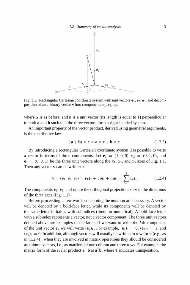
Fig. 1.1. Rectangular Cartesian coordinate system with unit vectorse1,e2,e3, and decom-position of an arbitrary vectorv into componentsv1, v2, v3.

whereα is as before, andn is a unit vector (its length is equal to 1) perpendicularto botha andb such that the three vectors form a right-handed system.An important property of the vector product, derived using geometric arguments,

is the distributive law

(a+ b)× c= a× c+ b× c. (1.2.3)

By introducing a rectangular Cartesian coordinate system it is possible to writea vector in terms of three components. Lete1 = (1,0,0), e2 = (0,1,0), ande3 = (0,0,1) be the three unit vectors along thex1, x2, andx3 axes of Fig. 1.1.Then any vectorv can be written as

v = (v1, v2, v3) = v1e1 + v2e2 + v3e3 =3∑i=1

viei . (1.2.4)

The componentsv1, v2, andv3 are the orthogonal projections ofv in the directionsof the three axes (Fig. 1.1).Before proceeding, a few words concerning the notation are necessary. A vector

will be denoted by a bold-face letter, while its components will be denoted bythe same letter in italics with subindices (literal or numerical). A bold-face letterwith a subindex represents a vector, not a vector component. The three unit vectorsdefined above are examples of the latter. If we want to write thekth componentof the unit vectorej we will write (ej )k. For example,(e2)1 = 0, (e2)2 = 1, and(e2)3 = 0. In addition, although vectors will usually be written in row form (e.g., asin (1.2.4)), when they are involved in matrix operations they should be consideredas column vectors, i.e., as matrices of one column and three rows. For example, thematrix form of the scalar producta · b is aTb, where T indicates transposition.


When the scalar product is applied to the unit vectors we find

e1 · e2 = e1 · e3 = e2 · e3 = 0 (1.2.5)

e1 · e1 = e2 · e2 = e3 · e3 = 1. (1.2.6)

Equations (1.2.5) and (1.2.6) can be summarized as follows:

ei · ej = δi j ={1, i = j0, i �= j .

(1.2.7)

The symbolδ jk is known as theKronecker delta, which is an example of a second-order tensor, and will play an important role in this book. As an example of (1.2.7),e2 · ek is zero unlessk = 2, in which case the scalar product is equal to 1.Next we derive an alternative expression for a vectorv. Using (1.2.4), the scalar

product ofv andei is

v · ei =(

3∑k=1

vkek

)· ei =

3∑k=1

vkek · ei =3∑k=1

vk(ek · ei ) = vi . (1.2.8)

Note that when applying (1.2.4) the subindex in the summation must be differentfrom i . To obtain (1.2.8) the following were used: the distributive law of the scalarproduct, the law of the product by a scalar, and (1.2.7). Equation (1.2.8) shows thatthe i th component ofv can be written as

vi = v · ei . (1.2.9)

When (1.2.9) is introduced in (1.2.4) we find

v =3∑i=1(v · ei )ei . (1.2.10)

This expression will be used in the discussion of dyadics (see §1.6).In terms of its components the length of the vector is given by

|v| =√v21 + v22 + v23 = (v · v)1/2. (1.2.11)

Using purely geometric arguments it is found that the scalar and vector productscan be written in component form as follows:

u · v = u1v1 + u2v2 + u3v3 (1.2.12)

and

u× v = (u2v3 − u3v2)e1 + (u3v1 − u1v3)e2 + (u1v2 − u2v1)e3. (1.2.13)

The last expression is based on the use of (1.2.3).

1.2 Summary of vector analysis 5

Vectors, and vector operations such as the scalar and vector products, among oth-ers, are defined independently of any coordinate system. Vector relations derivedwithout recourse to vector components will be valid when written in componentform regardless of the coordinate system used. Of course, the same vector may(and generally will) have different components in different coordinate systems,but they will represent the same geometric entity. This is true for Cartesian andmore general coordinate systems, such as spherical and cylindrical ones, but in thefollowing we will consider the former only.Now suppose that we want to define new vector entities based on operations on

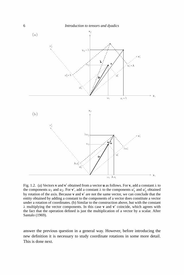
the components of other vectors. In view of the comments in §1.1 it is reasonableto expect that not every arbitrary definition will represent a vector, i.e., an entityintrinsically independent of the coordinate system used to represent the space. Tosee this consider the following example, which for simplicity refers to vectors intwo-dimensional (2-D) space. Given a vectoru = (u1,u2), define a new vectorv = (u1 + λ,u2 + λ), whereλ is a nonzero scalar. Does this definition result ina vector? To answer this question draw the vectorsu andv (Fig. 1.2a), rotate theoriginal coordinate axes, decomposeu into its new componentsu′

1 andu′2, addλ

to each of them, and draw the new vectorv′ = (u′1 + λ,u′

2 + λ). Clearly,v andv′

are not the same geometric object. Therefore, our definition does not represent avector.Now consider the following definition:v = (λu1, λu2). After a rotation similar

to the previous one we see thatv = v′ (Fig. 1.2b), which is not surprising, as thisdefinition corresponds to the multiplication of a vector by a scalar.Let us look now at a more complicated example. Suppose that given two vectors

u andv we want to define a third vectorw as follows:

w = (u2v3 + u3v2)e1 + (u3v1 + u1v3)e2 + (u1v2 + u2v1)e3. (1.2.14)

Note that the only difference with the vector product (see (1.2.13)) is the re-placement of the minus signs by plus signs. As before, the question is whether thisdefinition is independent of the coordinate system. In this case, however, finding ananswer is not straightforward. What one should do is to compute the componentsw1, w2, w3 in the original coordinate system, draww, perform a rotation of axes,find the new components ofu andv, computew′

1,w′2, andw

′3, draww

′ and compareit with w. If it is found that the two vectors are different, then it is obvious that(1.2.14) does not define a vector. If the two vectors are equal it might be temptingto say that (1.2.14) does indeed define a vector, but this conclusion would not becorrect because there may be other rotations for whichw andw′ are not equal.These examples should convince the reader that establishing the vectorial char-

acter of an entity defined by its components requires a definition of a vector thatwill take this question into account automatically. Only then will it be possible to


Fig. 1.2. (a) Vectorsv andv′ obtained from a vectoru as follows. Forv, add a constantλ tothe componentsu1 andu2. Forv′, add a constantλ to the componentsu′

1 andu′2 obtained

by rotation of the axis. Becausev andv′ are not the same vector, we can conclude that theentity obtained by adding a constant to the components of a vector does constitute a vectorunder a rotation of coordinates. (b) Similar to the construction above, but with the constantλ multiplying the vector components. In this casev andv′ coincide, which agrees withthe fact that the operation defined is just the multiplication of a vector by a scalar. AfterSantalo (1969).

answer the previous question in a general way. However, before introducing thenew definition it is necessary to study coordinate rotations in some more detail.This is done next.

1.3 Rotation of Cartesian coordinates. Definition of a vector 7

1.3 Rotation of Cartesian coordinates. Definition of a vector

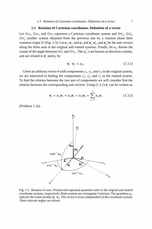
Let Ox1, Ox2, andOx3 represent a Cartesian coordinate system andOx′1, Ox′2,

Ox′3 another system obtained from the previous one by a rotation about theircommon originO (Fig. 1.3). Lete1, e2, ande3 ande′1, e

′2, ande

′3 be the unit vectors

along the three axes in the original and rotated systems. Finally, letai j denote thecosine of the angle betweenOx′i andOxj . Theai j ’s are known as direction cosines,and are related toe′i andej by

e′i · ej = ai j . (1.3.1)

Given an arbitrary vectorvwith componentsv1, v2, andv3 in the original system,we are interested in finding the componentsv′

1, v′2, andv

′3 in the rotated system.

To find the relation between the two sets of components we will consider first therelation between the corresponding unit vectors. Using (1.3.1)e′i can be written as

e′i = ai1e1 + ai2e2 + ai3e3 =3∑j=1

ai j ej (1.3.2)

(Problem 1.3a).

Fig. 1.3. Rotation of axes. Primed and unprimed quantities refer to the original and rotatedcoordinate systems, respectively. Both systems are rectangular Cartesian. The quantitiesai jindicate the scalar producte′i ·ej . The vectorv exists independent of the coordinate system.Three relevant angles are shown.


Furthermore, in the original and rotated systemsv can be written as

v =3∑j=1v jej (1.3.3)

and

v =3∑i=1

v′ie

′i . (1.3.4)

Now introduce (1.3.2) in (1.3.4)

v =3∑i=1

v′i

3∑j=1

ai j ej ≡3∑j=1

(3∑i=1

ai j v′i

)ej . (1.3.5)

Since (1.3.3) and (1.3.5) represent the same vector, and the three unit vectorse1,e1, ande3 are independent of each other, we conclude that

v j =3∑i=1

ai j v′i . (1.3.6)

If we write theej s in terms of thee′i s and replace them in (1.3.3) we find that

v′i =

3∑j=1

ai j v j (1.3.7)

(Problem 1.3b).Note that in (1.3.6) the sum is over the first subindex ofai j , while in (1.3.7)

the sum is over the second subindex ofai j . This distinction is critical and must berespected.Now we are ready to introduce the following definition of a vector:

three scalars are the components of a vector if under a rotation of coordinates they trans-form according to (1.3.7).

What this definition means is that if we want to define a vector by some setof rules, we have to verify that the vector components satisfy the transformationequations.Before proceeding we will introduce asummation convention(due to Einstein)

that will simplify the mathematical manipulations significantly. The conventionapplies to monomial expressions (such as a single term in an equation) and consistsof dropping the sum symbol and summing over repeated indices.1 This conventionrequires that the same index should appear no more than twice in the same term.

1 In this book the convention will not be applied to uppercase indices

1.3 Rotation of Cartesian coordinates. Definition of a vector 9

Repeated indices are known asdummy indices, while those that are not repeatedare calledfree indices. Using this convention, we will write, for example,

v =3∑j=1v jej = v jej (1.3.8)

v j =3∑i=1

ai j v′i = ai j v

′i (1.3.9)

v′i =

3∑j=1

ai j v j = ai j v j . (1.3.10)

It is important to have a clear idea of the difference between free and dummyindices. A particular dummy index can be changed at will as long as it is replaced(in its two occurrences) by some other index not equal to any other existing indicesin the same term. Free indices, on the other hand, are fixed and cannot be changedinside a single term. However, a free index can be replaced by another as long asthe change is effected in all the terms in an equation, and the new index is differentfrom all the other indices in the equation. In (1.3.9)i is a dummy index andj is afree index, while in (1.3.10) their role is reversed. The examples below show legaland illegal index manipulations.The following relations, derived from (1.3.9), are true

v j = ai j v′i = akjv

′k = al j v

′l (1.3.11)

because the repeated indexi was replaced by a different repeated index (equal tok or l ). However, it would not be correct to replacei by j becausej is alreadypresent in the equation. Ifi were replaced byj we would have

v j = aj j v′j , (1.3.12)

which would not be correct because the indexj appears more than twice in theright-hand term, which is not allowed. Neither would it be correct to write

v j = aikv′i (1.3.13)

because the free indexj has been changed tok only in the right-hand term. On theother hand, (1.3.9) can be written as

vk = aikv′i (1.3.14)

because the free indexj has been replaced byk on both sides of the equation.As (1.3.9) and (1.3.10) are of fundamental importance, it is necessary to pay

attention to the fact that in the former the sum is over the first index ofai j while


in the latter the sum is over the second index ofai j . Also note that (1.3.10) can bewritten as the product of a matrix and a vector:

v′ =

v′1

v′2

v′3

=a11 a12 a13a21 a22 a23a31 a32 a33

v1v2v3

≡ Av, (1.3.15)

whereA is the matrix with elementsai j .It is clear that (1.3.9) can be written as

v = ATv′, (1.3.16)

where the superscript T indicates transposition.Now we will derive an important property ofA. By introducing (1.3.10) in

(1.3.9) we obtain

v j = ai j aikvk. (1.3.17)

Note that it was necessary to change the dummy index in (1.3.10) to satisfy thesummation convention. Equation (1.3.17) implies that any of the three componentsof v is a combination of all three components. However, this cannot be generallytrue becausev is an arbitrary vector. Therefore, the right-hand side of (1.3.17) mustbe equal tov j , which in turn implies that the productai j aik must be equal to unitywhen j = k, and equal to zero whenj �= k. This happens to be the definition ofthe Kronecker deltaδ jk introduced in (1.2.7), so that

ai j aik = δ jk . (1.3.18)

If (1.3.9) is introduced in (1.3.10) we obtain

ai j ak j = δik . (1.3.19)

Settingi = k in (1.3.19) and writing in full gives

1= a2i1 + a2i2 + a2i3 = |e′i |2; i = 1,2,3, (1.3.20)

where the equality on the right-hand side follows from (1.3.2).Wheni �= k, (1.3.19) gives

0= ai1ak1 + ai2ak2 + ai3ak3 = e′i · e′k, (1.3.21)

where the equality on the right-hand side also follows from (1.3.2). Therefore,(1.3.19) summarizes the fact that thee′j s are unit vectors orthogonal to each other,while (1.3.18) does the same thing for theei s. Any set of vectors having theseproperties is known as an orthonormal set.

1.4 Cartesian tensors 11

In matrix form, (1.3.18) and (1.3.19) can be written as

ATA = AAT = I , (1.3.22)

whereI is the identity matrix.Equation (1.3.22) can be rewritten in the following useful way:

AT = A−1; (AT)−1 = A, (1.3.23)

where the superscript−1 indicates matrix inversion. From (1.3.22) we also find

|AAT| = |A||AT| = |A|2 = |I | = 1, (1.3.24)

where vertical bars indicate the determinant of a matrix.Linear transformations with a matrix such that its determinant squared is equal

to 1 are known as orthogonal transformations. When|A| = 1, the transformationcorresponds to a rotation. When|A| = −1, the transformation involves the reflec-tion of one coordinate axis in a coordinate plane. An example of reflection is thetransformation that leaves thex1 andx2 axes unchanged and replaces thex3 axisby −x3. Reflections change the orientation of the space: if the original system isright-handed, then the new system is left-handed, and vice versa.

1.4 Cartesian tensors

In subsequent chapters the following three tensors will be introduced.

(1) The strain tensorεi j :

εi j = 1

2

(∂ui∂xj

+ ∂u j∂xi

); i, j = 1,2,3, (1.4.1)

where the vectoru = (u1,u2,u3) is the displacement suffered by a particleinside a body when it is deformed.

(2) The stress tensorτi j :

Ti = τi j n j ; i = 1,2,3, (1.4.2)

whereTi andnj indicate the components of the stress vector and normal vectorreferred to in §1.1.

(3) The elastic tensorci jkl , which relates stress to strain:

τi j = ci jkl εkl . (1.4.3)

Let us list some of the differences between vectors and tensors. First, while avector can be represented by a single symbol, such asu, or by its components,such asu j , a tensor can only be represented by its components (e.g.,εi j ), althoughthe introduction of dyadics (see §1.6) will allow the representation of tensors by


single symbols. Secondly, while vector components carry only one subindex, ten-sors carry two subindices or more. Thirdly, in the three-dimensional space we areconsidering, a vector has three components, whileεi j andτi j have 3× 3, or nine,components, andci jkl has 81 components (3× 3× 3× 3). Tensorsεi j andτi j areknown as second-order tensors, whileci jkl is a fourth-order tensor, with the orderof the tensor being given by the number of free indices. There are also differencesamong the tensors shown above. For example,εi j is defined in terms of operations(derivatives) on the components of a single vector, whileτi j appears in a relationbetween two vectors.ci jkl , on the other hand, relates two tensors.Clearly, tensors offer more variety than vectors, and because they are defined in

terms of components, the comments made in connection with vector componentsand the rotation of axes also apply to tensors. To motivate the following definitionof a second-order tensor consider the relation represented by (1.4.2). For this rela-tion to be independent of the coordinate system, upon a rotation of axes we musthave

T ′l = τ ′

lkn′k. (1.4.4)

In other words, the functional form of the relation must remain the same after achange of coordinates. We want to find the relation betweenτ ′

lk andτi j that satisfies(1.4.2) and (1.4.4). To do that multiply (1.4.2) byali and sum overi :

ali Ti = ali τi j n j . (1.4.5)

Before proceeding rewriteT ′l andnj using (1.3.10) withv replaced byT and (1.3.9)

with v replaced byn. This gives

T ′l = ali Ti ; nj = akjn

′k. (1.4.6a,b)

From (1.4.6a,b), (1.4.2), and (1.4.5) we find

T ′l = ali Ti = ali τi j n j = ali τi j ak jn

′k = (ali ak jτi j )n

′k. (1.4.7)

Now subtracting (1.4.4) from (1.4.7) gives

0= (τ ′lk − ali ak jτi j )n

′k. (1.4.8)

As nk is an arbitrary vector, the factor in parentheses in (1.4.8) must be equal tozero (Problem 1.7), so that

τ ′lk = ali ak jτi j . (1.4.9)

Note that (1.4.9) does not depend on the physical nature of the quantities involvedin (1.4.2). Only the functional relation matters. This result motivates the followingdefinition.


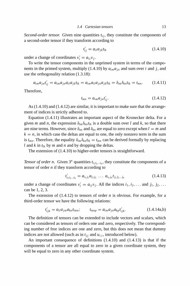
Second-order tensor.Given nine quantitiesti j , they constitute the components ofa second-order tensor if they transform according to

t ′i j = ail ajktlk (1.4.10)

under a change of coordinatesv′i = ai j v j .

To write the tensor components in the unprimed system in terms of the compo-nents in the primed system, multiply (1.4.10) byaimajn and sum overi and j , anduse the orthogonality relation (1.3.18):

aimajnt′i j = aimajnail ajktlk = aimail ajnajktlk = δlmδkntlk = tmn. (1.4.11)

Therefore,

tmn = aimajnt′i j . (1.4.12)

As (1.4.10) and (1.4.12) are similar, it is important to make sure that the arrange-ment of indices is strictly adhered to.Equation (1.4.11) illustrates an important aspect of the Kronecker delta. For a

givenm andn, the expressionδlmδkntlk is a double sum overl andk, so that thereare nine terms. However, sinceδlm andδkn are equal to zero except whenl = mandk = n, in which case the deltas are equal to one, the only nonzero term in the sumis tmn. Therefore, the equalityδlmδkntlk = tmn can be derived formally by replacingl andk in tlk bym andn and by dropping the deltas.The extension of (1.4.10) to higher-order tensors is straightforward.

Tensor of order n.Given 3n quantitiesti1i2...in , they constitute the components of atensor of ordern if they transform according to

t ′i1i2...in = ai1 j1ai2 j2 . . . ain jn t j1 j2... jn (1.4.13)

under a change of coordinatesv′i = ai j v j . All the indicesi1, i2, . . . and j1, j2, . . .

can be 1, 2, 3.The extension of (1.4.12) to tensors of ordern is obvious. For example, for a

third-order tensor we have the following relations:

t ′i jk = ail ajmakntlmn; tmnp= aimajnakpt′i jk . (1.4.14a,b)

The definition of tensors can be extended to include vectors and scalars, whichcan be considered as tensors of orders one and zero, respectively. The correspond-ing number of free indices are one and zero, but this does not mean that dummyindices are not allowed (such as int j j andui,i , introduced below).An important consequence of definitions (1.4.10) and (1.4.13) is that if the

components of a tensor are all equal to zero in a given coordinate system, theywill be equal to zero in any other coordinate system.


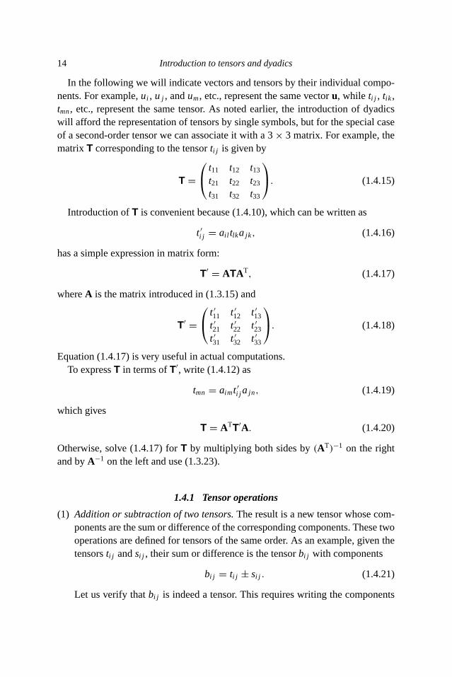
In the following we will indicate vectors and tensors by their individual compo-nents. For example,ui , u j , andum, etc., represent the same vectoru, while ti j , tik ,tmn, etc., represent the same tensor. As noted earlier, the introduction of dyadicswill afford the representation of tensors by single symbols, but for the special caseof a second-order tensor we can associate it with a 3× 3 matrix. For example, thematrixT corresponding to the tensorti j is given by

T = t11 t12 t13t21 t22 t23t31 t32 t33

. (1.4.15)

Introduction ofT is convenient because (1.4.10), which can be written as

t ′i j = ail tlkajk, (1.4.16)

has a simple expression in matrix form:

T′ = ATAT, (1.4.17)

whereA is the matrix introduced in (1.3.15) and

T′ = t ′11 t ′12 t ′13t ′21 t ′22 t ′23t ′31 t ′32 t ′33

. (1.4.18)

Equation (1.4.17) is very useful in actual computations.To expressT in terms ofT′, write (1.4.12) as

tmn = aimt′i j ajn, (1.4.19)

which gives

T = ATT′A. (1.4.20)

Otherwise, solve (1.4.17) forT by multiplying both sides by(AT)−1 on the rightand byA−1 on the left and use (1.3.23).

1.4.1 Tensor operations

(1) Addition or subtraction of two tensors.The result is a new tensor whose com-ponents are the sum or difference of the corresponding components. These twooperations are defined for tensors of the same order. As an example, given thetensorsti j andsi j , their sum or difference is the tensorbi j with components

bi j = ti j ± si j . (1.4.21)

Let us verify thatbi j is indeed a tensor. This requires writing the components


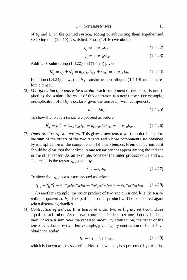
of ti j andsi j in the primed system, adding or subtracting them together andverifying that (1.4.10) is satisfied. From (1.4.10) we obtain

t ′i j = ail ajmtlm (1.4.22)

s′i j = ail ajmslm. (1.4.23)

Adding or subtracting (1.4.22) and (1.4.23) gives

b′i j = t ′i j ± s′i j = ail ajm(tlm ± slm) = ail ajmblm. (1.4.24)

Equation (1.4.24) shows thatbi j transforms according to (1.4.10) and is there-fore a tensor.

(2) Multiplication of a tensor by a scalar.Each component of the tensor is multi-plied by the scalar. The result of this operation is a new tensor. For example,multiplication ofti j by a scalarλ gives the tensorbi j with components

bi j = λti j . (1.4.25)

To show thatbi j is a tensor we proceed as before

b′i j = λt ′i j = λail ajmtlm = ail ajm(λtlm) = ail ajmblm. (1.4.26)

(3) Outer product of two tensors.This gives a new tensor whose order is equal tothe sum of the orders of the two tensors and whose components are obtainedby multiplication of the components of the two tensors. From this definition itshould be clear that the indices in one tensor cannot appear among the indicesin the other tensor. As an example, consider the outer product ofti j anduk.The result is the tensorsi jk given by

si jk = ti j uk. (1.4.27)

To show thatsi jk is a tensor proceed as before

s′i jk = t ′i j u′k = ail ajmtlmaknun = ail ajmakntlmun = ail ajmaknslmn. (1.4.28)

As another example, the outer product of two vectorsa andb is the tensorwith componentsai bj . This particular outer product will be considered againwhen discussing dyadics.

(4) Contraction of indices.In a tensor of order two or higher, set two indicesequal to each other. As the two contracted indices become dummy indices,they indicate a sum over the repeated index. By contraction, the order of thetensor is reduced by two. For example, giventi j , by contraction ofi and j weobtain the scalar

ti i = t11+ t22+ t33, (1.4.29)

which is known as thetraceof ti j . Note that whenti j is represented by amatrix,


ti i corresponds to the sum of its diagonal elements, which is generally knownas the trace of the matrix. Another example of contraction is the divergence ofa vector, discussed in §1.4.5.

(5) Inner product, or contraction, of two tensors.Given two tensors, first formtheir outer product and then apply a contraction of indices using one indexfrom each tensor. For example, the scalar product of two vectorsa andb isequal to their inner product, given byai bi . We will refer to the inner productas the contraction of two tensors. By extension, a product involvingai j , as in(1.4.5) and (1.4.11), for example, will also be called a contraction.

1.4.2 Symmetric and anti-symmetric tensors

A second-order tensorti j is symmetric if

ti j = t j i (1.4.30)

and anti-symmetric if

ti j = −t j i . (1.4.31)

Any second-order tensorbi j can be written as the following identity:

bi j ≡ 1

2bi j + 1

2bi j + 1

2bji − 1

2bji = 1

2(bi j + bji )+ 1

2(bi j − bji ). (1.4.32)

Clearly, the tensors in parentheses are symmetric and anti-symmetric, respectively.Therefore,bi j can be written as

bi j = si j + ai j (1.4.33)

with

si j = sji = 1

2(bi j + bji ) (1.4.34)

and

ai j = −aji = 1

2(bi j − bji ). (1.4.35)

Examples of symmetric second-order tensors are the Kronecker delta, the straintensor (as can be seen from (1.4.1)), and the stress tensor, as will be shown in thenext chapter.For higher-order tensors, symmetry and anti-symmetry are referred to pairs of

indices. A tensor is completely symmetric (anti-symmetric) if it is symmetric (anti-symmetric) for all pairs of indices. For example, ifti jk is completely symmetric,then

ti jk = t j ik = tik j = tk j i = tki j = t jki . (1.4.36)


If ti jk is completely anti-symmetric, then

ti jk = −t j ik = −tik j = tki j = −tk j i = t jki . (1.4.37)

The permutation symbol, introduced in §1.4.4, is an example of a completely anti-symmetric entity.The elastic tensor in (1.4.3) has symmetry properties different from those de-

scribed above. They will be described in detail in Chapter 4.

1.4.3 Differentiation of tensors

Let ti j be a function of the coordinatesxi (i = 1, 2, 3). From (1.4.10) we know that

t ′i j = aikajl tkl . (1.4.38)

Now differentiate both sides of (1.4.38) with respect tox′m,

∂t ′i j∂x′

m

= aikajl∂tkl∂xs

∂xs∂x′

m

. (1.4.39)

Note that on the right-hand side we used the chain rule of differentiation and thatthere is an implied sum over the indexs. Also note that since

xs = amsx′m (1.4.40)

(Problem 1.8) then

∂xs∂x′

m

= ams. (1.4.41)

Using (1.4.41) and introducing the notation

∂t ′i j∂x′

m

≡ t ′i j ,m; ∂tkl∂xs

≡ tkl,s (1.4.42)

equation (1.4.39) becomes

t ′i j ,m = aikajl amstkl,s. (1.4.43)

This shows thattkl,s is a third-order tensor.Applying the same arguments to higher-order tensors shows that first-order dif-

ferentiation generates a new tensor with the order increased by one. It must beemphasized, however, that in general curvilinear coordinates this differentiationdoes not generate a tensor.


1.4.4 The permutation symbol

This is indicated byεi jk and is defined by

εi jk =

0, if any two indices are repeated1, if i jk is an even permutation of 123

−1, if i jk is an odd permutation of 123.(1.4.44)

A permutation is even (odd) if the number of exchanges ofi, j, k required toorder them as 123 is even (odd). For example, to go from 213 to 123 only oneexchange is needed, so the permutation is odd. On the other hand, to go from 231to 123, two exchanges are needed: 231→ 213 → 123, and the permutation iseven. After considering all the possible combinations we find

ε123= ε231= ε312= 1 (1.4.45)

ε132= ε321= ε213= −1. (1.4.46)

The permutation symbol is also known as the alternating or Levi-Civita symbol.The definition (1.4.44) is general in the sense that it can be extended to more thanthree subindices. The following equivalent definition can only be used with threesubindices, but is more convenient for practical uses:

εi jk =

0, if any two indices are repeated1, if i jk are in cyclic order

−1, if i jk are not in cyclic order.(1.4.47)

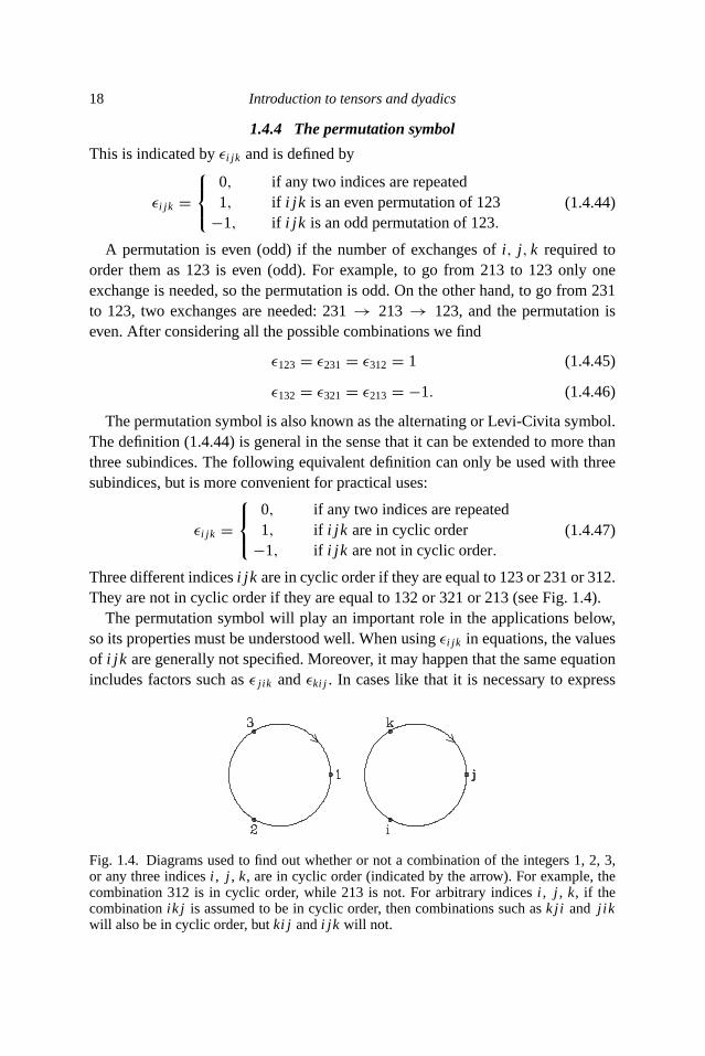
Three different indicesi jk are in cyclic order if they are equal to 123 or 231 or 312.They are not in cyclic order if they are equal to 132 or 321 or 213 (see Fig. 1.4).The permutation symbol will play an important role in the applications below,

so its properties must be understood well. When usingεi jk in equations, the valuesof i jk are generally not specified. Moreover, it may happen that the same equationincludes factors such asε j ik andεki j . In cases like that it is necessary to express

Fig. 1.4. Diagrams used to find out whether or not a combination of the integers 1, 2, 3,or any three indicesi , j , k, are in cyclic order (indicated by the arrow). For example, thecombination 312 is in cyclic order, while 213 is not. For arbitrary indicesi , j , k, if thecombinationik j is assumed to be in cyclic order, then combinations such ask j i and j ikwill also be in cyclic order, butki j andi jk will not.


one of them in terms of the other. To do that assume thatj ik is in cyclic order(Fig. 1.4) and by inspection find out whetherki j is in the same order or not. As itis not,εki j = −ε j ik .Is the permutation symbol a tensor? Almost. If the determinant of the transfor-

mation matrixA is equal to 1, then the components ofεi jk transform accordingto (1.4.14a). However, if the determinant is equal to−1, the components ofεi jktransform according to−1 times the right-hand side of (1.4.14a). Entities withthis type of transformation law are known aspseudo tensors. Another well-knownexample is the vector product, which produces apseudo vector, rather than a vector.Another important aspect ofεi jk is that its components are independent of the

coordinate system (see §1.4.7). A proof of the tensorial character ofεi jk can befound in Goodbody (1982) and McConnell (1957).

1.4.5 Applications and examples

In the following it will be assumed that the scalars, vectors, and tensors are func-tions ofx1, x2, andx3, as needed, and that the required derivatives exist.

(1) By contraction of the second-order tensorui, j we obtain the scalarui,i . Whenthis expression is written in full it is clear that it corresponds to thedivergenceof u:

ui,i = ∂u1∂x1

+ ∂u2∂x2

+ ∂u3∂x3

= div u = ∇ · u. (1.4.48)

In the last term we introduced the vector operator∇ (nabla or del), which canbe written as

∇ =(∂

∂x1,∂

∂x2,∂

∂x3

). (1.4.49)

This definition of∇ is valid in Cartesian coordinate systems only.

(2) The derivative of the scalar functionf (x1, x2, x3) with respect toxi is thei thcomponent of thegradientof f :

∂ f

∂xi= (∇ f )i = f,i . (1.4.50)

(3) The sum of second derivativesf,i i of a scalar functionf is theLaplacianoff :

f,i i = ∂2 f

∂x21+ ∂2 f

∂x22+ ∂2 f

∂x23= ∇2 f. (1.4.51)


(4) The second derivatives of the vector componentsui areui, jk . By contractionwe obtainui, j j , which corresponds to thei th component of the Laplacian ofthe vectoru:

∇2u = (∇2u1,∇2u2,∇2u3) = (

u1, j j ,u2, j j ,u3, j j). (1.4.52)

Again, this definition applies to Cartesian coordinates only. In general orthog-onal coordinate systems theLaplacian of a vectoris defined by

∇2u = ∇(∇ · u)− ∇ × ∇ × u, (1.4.53)

where the appropriate expressions for the gradient, divergence, and curlshould be used (e.g., Morse and Feshbach, 1953; Ben-Menahem and Singh,1981). For Cartesian coordinates (1.4.52) and (1.4.53) lead to the same ex-pression (Problem 1.9).

(5) Show that the Kronecker delta is a second-order tensor. Let us apply thetransformation law (1.4.10):

δ′i j = ail ajkδlk = ail ajl = δi j . (1.4.54)

This shows thatδi j is a tensor. Note that in the term to the right of the firstequality there is a double sum overl andk (nine terms) but because of thedefinition of the delta, the only nonzero terms are those withl = k (threeterms), in which case delta has a value of one. The last equality comes from(1.3.19).

(6) Let B be the 3× 3 matrix with elementsbi j . Then, the determinant ofB isgiven by

|B| ≡∣∣∣∣∣∣b11 b12 b13b21 b22 b23b31 b32 b33

∣∣∣∣∣∣ = εi jk b1i b2 j b3k = εi jk bi1bj2bk3. (1.4.55)

The two expressions in terms ofεi jk correspond to the expansion of the deter-minant by rows and columns, respectively. It is straightforward to verify that(1.4.55) is correct. In fact, those familiar with determinants will recognizethat (1.4.55) is the definition of a determinant.

(7) Vector product ofu andv. Thei th component is given by

(u× v)i = εi jk u j vk. (1.4.56)

(8) Curl of a vector. Thei th component is given by

(curlu)i = (∇ × u)i = εi jk∂

∂xjuk = εi jk uk, j . (1.4.57)

elastic wave propagation and generation in...

Documents