elastodynamic and elastostatic green tensors for

Geophys. J . Int. (1997) 130,786-800

Elastodynamic and elastostatic Green tensors for homogeneous weak transversely isotropic media

Vaclav VavryEuk Geophysical Institute, Czech Academy of Sciences, BoCni 11,4401, 141 31 Praha 4, Czech Republic. E-mail: [email protected]

Accepted 1997 May 16. Received 1997 May 1 4 in original form 1996 June 6

SUMMARY An explicit analytical formula for the complete elastodynamic Green tensor for homogeneous unbounded weak transversely isotropic media is presented. The formula was derived by analytical calculations of higher-order approximations of the ray series. The ray series is finite and consists of seven non-zero terms. The formula for the Green tensor is complete and correct for the whole frequency range, thus it describes correctly the wavefield at all distances and at all directions including the shear-wave singularity direction. The Green tensor consists of P, SV and SH far-field waves and four coupling waves. Three of them couple P and SV waves, and the fourth wave couples the SV and SH waves. The P-SV coupling waves behave similarly to the near-field waves in isotropy. However, the SV-SH coupling wave, which is called 'shear-wave coupling', behaves exceptionally and it has no analogy in the Green tensor for isotropy. The formula for the elastostatic Green tensor is also derived.

Key words: anisotropy, Green tensor, perturbation methods, ray theory, shear-wave coupling, shear-wave splitting.

1 INTRODUCTION

The point-force solution of the elastodynamic equation for homogeneous isotropic media was found by Stokes (1849). This well-known solution, known as the elastodynamic Green tensor for homogeneous isotropic and unbounded media, plays a fundamental role in elastodynamics. For anisotropic media, however, the problem is much more complex. Christoffel(l877) solved for plane-wave propagation in anisotropic media, but the point-force solution was unsolved. More than 100 years after the original Stokes paper, Lighthill (1960) and Buchwald (1959) found an integral form of the Green tensor for homogeneous anisotropic media: Lighthill ( 1960) for magnetohydro- dynamics and Buchwald (1959) for elastodynamics. The Green tensor is expressed by the Fourier integral, and the integral can be solved by the stationary phase method under the far- field approximation. We will call this solution the far-field or high-frequency approximation of the Green tensor. The point- force solutions for anisotropic media were also studied by Duff (1960), Burridge (1967), Yeatts (1984), Kazi-Aoual, Bonnet & Jouanna (1988), Tverdokhlebov & Rose (1988) and Wang & Achenbach (1993, 1994), among others. The solutions in those papers were obtained by the Fourier, Laplace or Radon trans- forms. Unfortunately, the solutions in the above-mentioned papers are either far-field approximations, or they are obtained by numerical application of the inverse transform. In order to obtain an explicit analytical form for the complete elastodynamic Green tensor including near-field waves, the inverse

transform was also solved analytically, but under very limited conditions only: for 2-D transverse isotropy (Payton 1971, 1983), for 3-D transverse isotropy for a ray parallel to the symmetry axis (Payton 1977, 1983), and for 3-D transverse isotropy for the general direction of a ray (Ben-Menahem & Sena 1990). Except for the SH-wave part of the 3-D Green tensor for transversely isotropic media, the above-mentioned analytical solutions are, however, complicated, and they do not give a simple physical insight as, for example, the Stokes solution into waves in isotropic media.

The formula for the SH-wave Green tensor in transverse isotropy was also derived by VavryCuk & Yomogida (1996) but by another method, analytical calculation of higher-order approximations of the ray series. Assuming that the Green tensor can be expressed by the ray expansion, we can calculate higher-order terms of the expansion from the far-field approximation of the Green tensor. Recurrent formulae for the calculation of higher-order terms of the ray series are known as the basic equations of the ray theory. For anisotropic media they were derived by Babich (1961), and subsequently studied by cerveny (1972). VavryCuk & Yomogida (1995, 1996) solved these equations for point sources in homogeneous media and showed that the Green tensor can be expressed exactly by the ray expansion with a finite number of terms, at least for some special cases (isotropy, SH waves in transverse isotropy). In this paper, we use this approach to set up the formula for the elastodynamic and consequently the elastostatic Green tensor for weak transverse isotropy. Weak transverse isotropy is chosen

786 0 1997 RAS

Elastodynamic and elastostatic Green tensors 787

since wave propagation is much simpler in this case, and all basic quantities of wavefields can be simply calculated by the perturbation method (Cerveny 1982; Farra 1989; Jech & PSenEik 1989; Nowack & PSenEik 1991; Kiselev 1994; Sayers 1994). Moreover, weak anisotropy and, in particular, weak transverse isotropy are frequently encountered in exploration seismics (Thomsen 1986), thus our calculations are not only of theoretical relevance, but they are also relevant for practical applications.

2 METHOD

The elastodynamic Green tensor for homogeneous anisotropic media satisfies the equation

pG,n - C i j k l G k n , l j = s i n s ( x ) s ( t ) , (1) where Gin = Gi,(x, t ) is the symmetric tensor of the second rank, p is the density, cijkl is the elasticity tensor, sin is the Kronecker delta, and 6 ( t ) is the Dirac delta function. Einstein summation convention is applied, where repeated indices mean summation. Solving eq. (1) by the Fourier method (e.g. Lighthill 1960; Buchwald 1959; Burridge 1967) leads to the solution in the form of a sum of three symmetric tensors:

G&, t ) = G;(X, t ) + G ~ : ( x , t ) + G ~ : ( x , t ) , (2) corresponding to three waves, P, S1 and S2. We assume that each of these tensors can be expressed in a form of the ray series (Cerveny 1972; Cervenk, Molotkov & PSenEik 1977):

m

G ~ ( x , t ) = 1 U r ( K ) ( x ) f ( K ) ( t - ~ " ( x ) ) , K = O

(3)

where

K denotes the order of the approximation, W denotes the wavetype (P, S1 or S2), U K ( K ) ( ~ ) is the ray amplitude tensor, and 7W(x) is the traveltime. Eq. (3) is the ray expansion of the Green tensor GE(x, t ) . Since the next formulae are analogous for all three waves, P, S1 and S2, the superscript W will be omitted unless it causes confusion. Inserting formula (3) into ( 1 ) leads to a system of equations for the amplitude tensors U p :

Ni,(Ui:')-Mi,(UL:-1))+Li,(Uif-2))=0, (4)

referred to as the basic equations of the ray theory. The right- hand side of eq. (4) is zero, because we eliminated the source term present in eq.(l). Later, we will discuss a way of incorporating an effect of the source into the solution of eq. (4).

Differential tensor operators N,,, M j n and L,, in (4) are defined for homogeneous anisotropic media as follows:

( K ) - r, u'K) - u(F) Nj??(ukn 1- j k kn jn 3

M j n ( U f ? ) = a i j k l ( P i u!!?l +PI ui!?i + pi,l u!?) >

Ljn(u!$) = aijkl uif!il > ( 5 )

aijkl is the density normalized elasticity tensor, p i is the slowness vector, p is the slowness, ni is the unit phase normal vector, c is the phase velocity and rj, is the Christoffel tensor. Instead

of the Christoffel tensor rjk= aijklP;Pl, we will sometimes use a scaled Christoffel tensor r j k = aijklninl. Both tensors, rjk and rjk, are symmetric. The ray amplitudes Ui:) for K < 0 are equal to zero.

Formula (4) is a recurrent system of equations for all terms UL:), K 2 0 of the ray expansion (3). For the calculation of Uif), it is convenient to introduce the so-called additional and principal components Ui:)' and Ui:)ll of the ray amplitude U g ) : U ( K ) kn - - U ( K ) L kn + UL:)I1 (see Cerveny 1972, eqs 18a and b; Cerveny et al. 1977, eqs 5.11 and 5.12). The calculation of each term of the ray series U i f ) ( K 2 0) is performed in two steps. First, the additional component Ui:)L is calculated by a differentiation of the lower-order terms. For P waves, U;jK) l is expressed as follows (see cerveny et al. 1977, eqs 5.13 and 5.14; VavryEuk & Yomogida 1996, eq. 6):

Second, the principal component Ug)I1 is calculated by solving an ordinary differential equation called the transport equation. For P waves generated by point sources in homogeneous anisotropic media, the transport equation reads (VavryEuk & Yomogida 1996, eq. 8) dU;;O)l' u;;o'l'

+--0. for K = O . a7 7

d~;;K)ll u P ( K ) I I kn +-

dz 7

= T { L , ( U ; ~ ~ - ~ ' ) - M , ( U ; ; ~ ) ~ ) } ~ ~ ~ ; , 1 for K > O . (6c)

The transport equations (6b and c) can be solved explicitly, and integration constants appearing in the solution can be determined (VavryCuk & Yomogida 1996, eq. 16). Finally, we can summarize the formulae for all terms U;LK) of the P-wave ray expansion: u;P&K) = u P ( K ) I + ~ f " K ) l l

for K < 0 : kn kn 3

U;;K)L = U;AK)l1 = 0,

for K=O:

(7) for K > 0 :

A;" = Afn(N) is the P-wave zeroth-order radiation function defined as the amplitude distribution on a sphere (but not on a wave surface), N is the ray direction, 1/47tp is a normalization constant, r is the distance of an observation point from the source, GW is an eigenvalue of the Christoffel tensor rj, and g"' is the corresponding unit polarization vector. The eigenvalue G P is equal to 1.

Forms of the function f ( ' ) ( t ) in eq. (3) and of the radiation function A;" in eq. (7) are not predicted by the theory presented

0 1997 RAS, GJI 130, 786-800

788 K VuuryCuk

because we eliminated a source term in eq.(4). Thus, the functions f ( ' ) ( t ) and A;" must be found by another method. Taking into account that the zeroth-order ray approximation is equivalent to the far-jield approximation, we can determine f ( ' ) ( t ) and A:,, from the far-field Green tensor for homogeneous anisotropic media (Ben-Menahem, Gibson & Sena 1991, eq. 12; Kendall, Guest & Thomson 1992, eq. 1; Ben-Menahem & Gibson 1995, eq. 51):

1 1 dd G;~(x, t ) = - - 6( t - ZP(X))

47.v (UP),@ T P

where u is the group velocity, K , and K , are the Gaussian curvatures of the slowness and wave surfaces, respectively, and 6 ( t ) is the Dirac delta function. Formula (8) was obtained by solving the exact integral form of the Green tensor by the stationary-phase method. G:p is also known as the ray- theoretical Green tensor. In fact, it is the zeroth-order ray- theoretical Green tensor in our terminology. Comparing eq. (8) with eqs (3) and (7), we obtain the following:

f " ) ( t ) = 6 ( t ) , A P - A - k'- UP@ g'g' - UP(PP)2*dd. (9)

Eqs ( 3 ) , (7) and (9) define a recurrent system of equations that allows us to find from the P-wave zeroth-order ray approximation, G::), all higher-order terms of the P-wave ray expansion, G:AK), K > 0. We can see that all the higher-order ray approximations can be obtained only by a spatial differentiation of the zeroth-order amplitude, U;;'), and by a time integration of I(')( t ) , which are mathematically elementary procedures. We should mention, however, that the multiple recursive differentiation tends to producing rather extensive formulae. Analogous formulae to eqs (7) and (9) can also be written for S1 and S2 waves.

3 WEAK T R A N S V E R S E ISOTROPY ( W T I )

3.1 Definition of WTI

We shall consider a weak transversely isotropic medium (hereafter called the WTI medium) with a vertical axis of rotation symmetry, defined as follows:

all = , a44 = 4 4 9 a13 = 4 3 + Aa13 >

(10) a33 = + A ~ 3 3 , Us6 = a24 + Aa66,

where a& = = 8,. a:" denotes the parameters of the unperturbed isotropic background medium with P and S velocities tl and /I, am" denotes the parameters of the WTI medium, and Aa,,, Au,, and are small perturbations satisfying conditions for weak anisotropy:

- 2a:,, ayl = t12 and

In (10) we do not perturb the parameters a,, and a44, since perturbations Aall and Aa44 do not cause anisotropy, but produce only perturbations of P and S velocities Atl and AD of an isotropic background medium. Thus, without any loss of generality, any WTI medium with a vertical axis of symmetry can be described by five parameters: P and S velocities in the

isotropic background tl and p, and perturbations Aa13, A u , ~ and AU66. Instead of the perturbations Aa,,, Aa,, and h6,, however, we will mainly use the anisotropy parameters E , , E~

and E,, defined as follows:

A ~ 3 3 - 2Aa13 Aa6fi and E , = - 2 2 ' E l = A ~ 1 3 , E2 =

thus

'11 + '33 - 2a13 - 4a44

2 = a13 - + 2~44, ~2 =

and

E3 = ___ a66 - a44

2 '

The reason for using the parameters E ~ , E~ and E, is the simplification of formulae presented later. The relations between parameters tl, fl, E ~ , E~ and E~ and Thomsen's parameters aT, PT, y, 6 and E (Thomsen 1986, eqs 8a,b, 9a,b and 17) are

tl=X,(l+E), p = f l ~ , E 1 = & $ ( 6 - 2 E ) ,

E 2 = W $ ( E - 6), (134

E3 = p$Y,

From (13) we can see that our isotropic background differs from that used by Thomsen (1986). The reason is that during the perturbation process we fixed the horizontal P-wave velocity (parameter a,,), but not the vertical P-wave velocity (parameter a,,), as done by Thomsen. Using eqs (13), we can readily express all the following formulae using Thomsen's parameters.

3.2 Perturbation formulae for WTI

The perturbation theory is a well-known method in theoretical physics (Morse & Feshbach 1953; Madelung 1964), in particular in quantum mechanics (Landau & Lifshitz 1974). We shall use it for calculating basic elastodynamic quantities for WTI media. Since the perturbation formulae for WTI are known (see e.g. Backus 1965; Thomsen 1986; Jech & PSenEik 1989; Kiselev 1994; Sayers 1994) or can be found without difficulty, we shall review them without any derivation. We shall present formulae for traveltimes, polarization vectors, eigenvalues of the Christoffel tensor, slowness vectors and Gaussian curvatures of the wave surface. All perturbed quantities will be expressed for a fixed ray direction specified by the unit vector N = (N, , N,, N,)T and by angle 0 between a ray and the symmetry axis.

(1) Phase velocities:

cP=tl a11

csv = p( 1 + - N ; - E2 " N : ) , a44 a44

0 1997 RAS, GJI 130, 786-800


(2) Traveltimes: (7) Gaussian curvatures of wave surfaces:

(3) P-wave polarization vector:

(4) Eigenvalues of the Christoffel tensor rkf:

a44

a44 a44

(5) Slowness vectors:

a44

(6) Angles between the ray and a phase normal:

E 6" = -2 sin 0 cos 0 2 ( 1 - 2N:), a44

E3

a44 hSH = 2 sin e cos e- .

4 THE ZEROTH-ORDER RAY APPROXIMATION OF THE GREEN TENSOR

Inserting perturbation formulae from the previous section into eq. (9), we obtain for the zeroth-order ray-theoretical Green tensor GLY)(x, t ) in WTI media the following formula:

(16)

The zeroth-order radiation functions Aff, A:,'' and A:? are defined as follows:

N:+ 1 + & 3 2 INkNf - N3(N16k3 + N k 6 f 3 )

a44( 1 - N:)

+6k3613-(1 - N:)6kf} > ( 224 where 6,, is the Kronecker delta. These formulae describe a linearized zeroth-order approximation of the Green tensor, valid only for weak anisotropy. The weaker the anisotropy, the better the formulae work. The Green tensor consists of three waves: P, SV and SH. All waves propagate with different velocities and have different polarizations. Velocities of P, SV

( 19)

0 1997 RAS, GJI 130, 786-800

790 V Vaury&k

and S H waves differ only slightly from the P- and S-wave velocities z and p of the isotropic background. Polarization of P waves also deviates slightly from the P-wave polarization in the background medium, which is parallel to the ray direction N. Polarizations of S waves in WTI, however, can differ from the S-wave polarization in the background medium quite distinctly. Instead of one S wave in isotropy, two S waves with mutually perpendicular polarizations propagate in WTI, SH-wave polarization being perpendicular to the axis of symmetry, and SV-wave polarization lying in the plane specified by the symmetry axis and a ray. The reason why the S-wave polarization in weakly anisotropic media is quite different from isotropy lies in the fact that anisotropy, in general, removes the degeneracy of S waves in isotropic media (see Jech & PSenEik 1989). The degeneracy of S waves is removed, even with weak anisotropy. The result is the well-known S-waoe splitting effect. Limits of the applicability of formulae (21) and (22) will be discussed later.

5 HIGHER-ORDER RAY APPROXIMATIONS OF THE GREEN TENSOR

Using formulae (21) and (22) for the zeroth-order ray-theoretical Green tensor for WTI and formulae (7) for higher-order terms of the ray expansion, we can recursively calculate the whole ray series of the WTI Green tensor for each P, S V and S H wave. This procedure is mathematically elementary since it involves only the partial derivatives of eq. (21). Nevertheless, since the differentiation is recursive, an extensive manipulation with rather complex formulae is needed. For this reason, we performed the calculations by using the symbolic manipulation software REDUCE (Hearn 1991). In this section, we will not present a detailed derivation, but will only summarize the basic formulae and general results. The final formula for the Green tensor including all higher-order ray approximations will be presented in the next section.

Calculating higher-order amplitude tensors U i . ) of the ray expansion for P, SV and SH waves, we arrive at the following results.

(1) For S H waves, the only non-zero higher-order term is the first-order term U;,"(l). All higher-order terms are equal to zero. For P and SV waves, six higher-order terms are non- zero and all the others are zero. A finite number of non-zero terms of the ray expansion of the P, SV and SH waves implies that the ray series is finite and convergent for all the three waves. Therefore, we can conclude that the Green tensor is expressed exactly by the ray series in the homogeneous WTI medium. This finding is very interesting and important, because the ray method is usually assumed to be only an approximate method, and the ray series is commonly assumed to be divergent.

(2) The first-order term for S H waves, U;,"(') contains none of the anisotropy parameters E~ or E ~ , and fully coincides with the first-order term, even for strong TI (see VavryEuk & Yomogida 1996, eq. 28). The first- and higher-order terms for P and SV waves contain no parameter E ~ . Moreover, the fifth- and sixth-order terms for P and SV waves do not contain the parameter E, .

(3) The third- and higher-order terms for P and SV waves are small perturbation quantities. This is obvious, since

amplitude tensors for the isotropic background medium UEl") are zero for K 2 3 (see VavryEuk & Yomogida 1995). Furthermore, calculation of the fifth- and sixth-order terms for P and SV waves simplifies considerably, because these terms are calculated from amplitude tensors, which are small perturbation quantities. In this case, the differential operators M,(ULf)) and L,(Uk.)) in eq. (7) reduce to operators for an isotropic background.

Formulae for the higher-order amplitude tensors U;fK) , Ufy;Y'K) and U;Fp'K) are rather extensive, thus we do not present them here. If we insert these tensors into the ray expansion (3), and take into account that the recursive integration of f " ) ( t ) yields

f'Q( t ) = 6( t ) , f'"( t ) = H ( t ) , + K - 1

f ' K ' ( t ) = L H ( t ) for K > 1 , (K - l)!

we can express formulae for the Green tensors G:[(x, t ) , G;;(x, t ) and GfF(x , t ) , and subsequently, for the complete Green tensor Gkl(x, t).

6 COMPLETE ELASTODYNAMIC GREEN TENSOR

The final form of the elastodynamic Green tensor for homogeneous WTI with the vertical axis of symmetry can be expressed as follows:

4," Bkf + ~ 6( t - Z S H ) -I- - [H( t - Ts") - H ( t - T S H ) ] r r2

(234

H ( t ) denotes the Heaviside step function, 6( t ) denotes the Dirac delta function, t is time, t = t(r, N) is the traveltime, r is the distance from an observation point to the source, and N is the ray direction. Using the time integrals instead of the Heaviside step function H ( t ) in eq. (23a), we get

123w

The zeroth-order radiation functions A;,, A:; and A:? are defined by eqs (22a-c). The higher-order radiation functions Bkl, C k l , Dk, and Ekl are defined as follows:

1 B -

Irf - /J'( 1 - N:)'

0 1997 RAS, GJI 130, 786-800


where a,, = a2 and a44 = B2. The correctness of the elastodynamic Green tensor was

verified by directly inserting (23) into the elastodynamic equation (1). For WTI with an arbitrarily oriented axis of symmetry, the Green tensor can be obtained from (23) by applying standard rules for the rotation of tensors.

For wavefield u(x, t ) generated by a generally oriented and time-dependent point force F(t), eq. (23b) yields

A;: A?? - 7') + -F,(t - 7s") + ---F,(t - P)

471P r r

For c1 = c2 = E~ = 0, eq. (23b) reduces to the exact formula for the elastodynamic Green tensor for homogeneous isotropic media:

7 PROPERTIES OF THE COMPLETE ELASTODYNAMIC GREEN TENSOR

Formulae (23) and (24) represent an explicit analytical form of the complete elastodynamic Green tensor for homogeneous WTI media. In contrast to the solution for general anisotropy (see e.g. Ben-Menahem & Gibson 1995, eq. 16) or for TI media

(see Ben-Menahem & Sena 1990), which are complicated, solution (23) is mathematically and computationally quite elementary. Moreover, it is very similar to the Stokes solurion for isotropic media. This enables us to understand the structure of the Green tensor for weak anisotropy and to obtain a physical insight into the differences between the Green tensor for isotropy and for weak anisotropy. We can study the properties of the different waves present in the Green tensor and understand which waves are dominant at different rays and at different distances from the source.

The Green tensor (23) consists of seven terms. The first three terms are the P, SV and SH waves in the zeroth-order ray approximation (hereafter the 'zeroth-order waves'), and the others are waves described by higher-order ray approximations (hereafter the 'higher-order waves'). The time dependence of the zeroth-order waves is the Dirac delta function, thus the amplitude of the waves is non-zero only at the instants of their arrivals. The amplitudes of the higher-order waves are non- zero at all times between the arrivals of the zeroth-order waves. The zeroth-order waves are high frequency, while the higher-order waves are rather low frequency. The amplitude of the zeroth-order waves decreases with distance as l/r; the amplitude of the higher-order waves decreases faster.

Radiation functions of the zeroth-order waves A:,, A:: and A:? consist of isotropic and anisotropic parts. The isotropic part is identical to the radiation functions of the Green tensor for isotropic media, and the anisotropic part is a linear function of the anisotropy parameter E,, E~ or E ~ . Since the anisotropy parameters must be small compared to elastic parameters of the isotropic background, anisotropic parts of the radiation functions represent only a small perturbation of the isotropic radiation functions. The higher-order radiation function C,, also consists of isotropic and anisotropic parts. However, the higher-order radiation functions &, and Ekl have no isotropic parts, thus they are zero for isotropic media. Functions Dk, and E,, are linear functions of the anisotropy parameters el and c2, but function Bk, does not depend on anisotropy parameters at all. For illustration, the isotropic and anisotropic parts of the zeroth-order and higher-order radiation functions in the x-z plane for vertical and horizontal single forces are shown in Figs 1 and 2. As expected, the anisotropic parts have, in general, more complicated forms than the isotropic parts, and are of a smaller amplitude than isotropic radiation functions. The exceptions are the radiation functions Dk, and E,,, which have relatively high amplitudes. This is due to scaling to the isotropic part of the radiation function C,,. However, functions D,, and Ek, stand at integrals which produce a function of lower frequencies and of a smaller amplitude than the integral standing at function Ckl. Thus these functions do not affect the amplitude of the Green tensor more significantly than the radiation function ckl. The most significant higher-order radiation function is function B,, , because this function is singular for a ray parallel to the symmetry axis. Exceptional properties of function B,, will be discussed in detail later.

As mentioned above, the higher-order waves occur only at times between the arrivals of the zeroth-order waves. We say that the higher-order waves couple the zeroth-order waves. This is mathematically displayed in eq. (23b) by the fact that the higher-order waves are expressed by integrals which couple terms of different ray expansions of P, SV and SH waves. Therefore, we can also call the higher-order waves coupling

0 1997 RAS, G J I 130, 786-800

792 I/. VavryEuk

Zeroth-order radiation functions

AiSO .-- . . A&,

. * - _ - s = 0.03

s = 0.03

P-SV higher-order radiation functions

C is0 %I ,-_ cE*

s = 0.03

1 ,

'-' s = O . l s = 0.1 I - $

.- , - E&2 I 3 D&, ! '

, ' . _ * s = 1

' , ' I ,. s = 8

~ horizontal force - - - - - - - - - - - vertical force

Figure I. Radiation functions for waves generated by the horizontal point single force F = (1,0, O)T (full line) and by the vertical point single force F = (0,0,1)= (dashed line). The magnitudes of the vector radiation functions are shown in the x-z plane. Parameters of the background medium: ul, = 22.36, u44 = 6.61. Ai,: the radiation function for far-field waves in the isotropic background; AC1 and AE2: parts of the radiation function A standing at anisotropy parameters zl and E ~ ; and analogously for functions C, D and E . Function ASH is zero for both forces. For the vertical force, function B is zero; for the horizontal force, B has the same form as shown in Fig. 2. Parameter s denotes the relative scale of anisotropic radiation functions with respect to the scale of the isotropic radiation function. Functions D and E have no isotropic parts Disa and Ei,,, thus D,,, D,,, E,, and E,, are scaled to the function CiJo. Function B is scaled to A::.

waves. For WTI media, we observe the coupling between P and SV waves and between SV and S H waves. Interestingly, no coupling between P and SH waves is observed. For general anisotropy, however, the coupling between all waves, P-S1, P-S2 and SlLS2, can be expected. The wave coupling is a typical phenomenon ignored by the zeroth-order ray theory, incorporated only by higher-order ray approximations. The coupling of higher-order waves is physically very important because it makes the Green tensor free from any static offset and divergence in time. Thus we can conclude that the higher- order waves in the Green tensor of any type of anisotropy

must be expressed only by coupling integrals similar to those in eq. (23b).

In the Green tensor for isotropic media (26), the zeroth- order waves describe the P and S waves in the far field, and the P-S coupling wave the wave in the near field (VavryEuk & Yomogida 1995). The far-field waves are dominant at distances greater than about 10 wavelengths from the source (see VavryEuk 1992), but for shorter distances the near-field waves should also be considered. Analogously in the Green tensor for WTI media (23b), the zeroth-order waves describe the P, SV and SH far-field waves, and the P-SV coupling

0 1997 RAS, GJI 130, 786-800


Zeroth-order and SV-SH higher-order radiation functions

A is0 A E3

SH 0 s = 0.2

P-SV higher-order radiation functions

Cis0 C&l

8 s = 0.1

B*(l-N(3)**2)

0 s = 3

CE2

s = 0.05

Figure 2. Radiation functions for waves generated by the horizontal single-point force F = (0, 1, O ) T . Radiation functions A' and As" are zero in the x-z plane. Function B is multiplied by the factor ( 1 - N g ) since B diverges for the ray direction N = (0, 0, l)T.

waves the near-field waves. However, the SV-SH coupling wave is exceptional in its properties. First, this wave is absent in the isotropic Green tensor because of the degeneracy of S waves in isotropic media. Second, its radiation function contains none of the anisotropy parameters c l , c2 or c 3 . The independence of radiation function BkI on strength of anisotropy indicates that the form of this wave will be preserved even for strong transverse isotropy. Third, since a time difference between the arrivals of shear waves (or, more exactly, quasi- shear waves) in weak anisotropy can be very small, the SV-SH coupling wave can be of relatively high frequency even at large distances from the source. Fourth, the radiation function B,, diverges for a ray parallel to the symmetry axis. For this reason, Fig. 2 does not show the SV-SH radiation function itself, but the function multiplied by a factor sin2 8, where 8 is the angle between a ray and the symmetry axis. For a direction parallel to the symmetry axis, velocities of SV and SH waves coincide, thus forming the shear-wave singularity. Although the amplitude of the SV-SH coupling wave decreases with distance generally as 1/r2, for the symmetry axis direction the dependence is changed into l / r due to the divergence of the radiation function for this direction. Moreover, the waveform of the coupling wave for this direction becomes the Dirac delta function, typical for waves in the far field. Thus, the complete Green tensor for the symmetry axis direction attains the following form:

+ 1 2 ~ ~ a , ~ a ~ ~ I ) r [ H ( t - r) - H ( t - ;)I, 1 a,, + 2 c 2 1 1

-6 t - - + G - ~ _ _ 4np a:, r ( :) 4np(a11 - a441

33 -

-24c2a11a44<}[H( r t - i) -H( t - ;)I. (27)

The other components of the Green tensor are zero. Formulae ( 2 7 ) are identical to Payton's analytical solution (Payton 1977) specified under weak anisotropy conditions ( 1 0 ) and ( 1 1 ) . It indicates that our approach gives correct results even for shear-wave singularity directions.

The term 'shear-wave coupling' or 'quasi-shear-wave coupling' was introduced and the phenomenon was first described by Chapman & Shearer (1989) and Coates & Chapman (1990), where an extensive discussion about the shear-wave coupling in inhomogeneous weakly anisotropic media can be found. In those papers, a method for calculating the shear-wave coupling due to gradients in weakly anisotropic

0 1997 RAS, GJI 130, 786-800

794 I/. Vavryc'uk

media is presented. In our paper, we found the S-wave coupling even in the Green tensor for homogeneous weakly anisotropic media. For a special case of weak anisotropy, we derived a very simple analytical formula for the S-wave coupling. We proved that the S-wave coupling in homogeneous media can be described by the ray theory correctly, if higher-order ray approximations are considered.

Limits of the applicability of the solution

In contrast to the exact solution of the Green tensor (see e.g. Ben-Menahem & Gibson 1995, eq. 16) valid for homogeneous general anisotropy (including strong anisotropy), formulae (23) are valid only for homogeneous weak transverse isotropy. By weak anisotropy we mean anisotropy that is free of caustics and that produces spatial variation of phase velocities up to 10 per cent. Some authors show that for some basic quantities (e.g. phase velocities) the weak anisotropy approximation works very well, even above the mentioned limit (see Jech & PSenCik 1989). However, the accuracy is reduced if the approxi- mated quantities are more complicated (e.g. polarization vectors, Gaussian curvatures, radiation functions). Except for

Phase velocities

Exact values

5.0 I I t

4.2 0 30 60 90

angle [degrees]

the weak anisotropy condition, no other approximation is used in the solution. Thus the solution describes correctly the wavefield at all distances from the source, including its close vicinity, and at all directions, including directions with shear- wave singularities. Note that directions with caustics are automatically excluded in weak anisotropy. The solution describes correctly the wavefield even in the limit of injinitely weak anisotropy, also called quasi-isotropy (Kravtsov & Orlov 1990).

8 NUMERICAL EXAMPLE

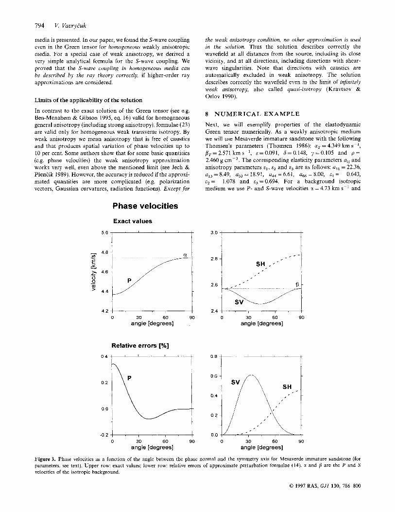
Next, we will exemplify properties of the elastodynamic Green tensor numerically. As a weakly anisotropic medium we will use Mesaverde immature sandstone with the following Thomsen's parameters (Thomsen 1986): aT = 4.349 km s-', bT=2.571 kms-', c=0.091, 6=0.148, y=0.105 and p = 2.460 g cm-3. The corresponding elasticity parameters aij and anisotropy parameters cl, E~ and E~ are as follows: a,, = 22.36,

c2 = - 1.078 and c3 = 0.694. For a background isotropic medium we use P- and S-wave velocities a = 4.73 km s-' and

a13 =z 8.49, a33 = 18.91, a44 = 6.61, a66 = 8.00, E l = -0.643,

2.6

2.4 0 30 60 90

angle [degrees]

Relative errors [%I

-0.2 0 30 60 90

angle [degrees]

0.0 I / 7 - , 1 4 0 30 60 90

angle [degrees]

Figure 3. Phase velocities as a function of the angle between the phase normal and the symmetry axis for Mesaverde immature sandstone (for parameters, see text). Upper row: exact values; lower row: relative errors of approximate perturbation formulae (14). c( and p are the P and S velocities of the isotropic background.

0 1997 RAS, GJI 130, 786-800


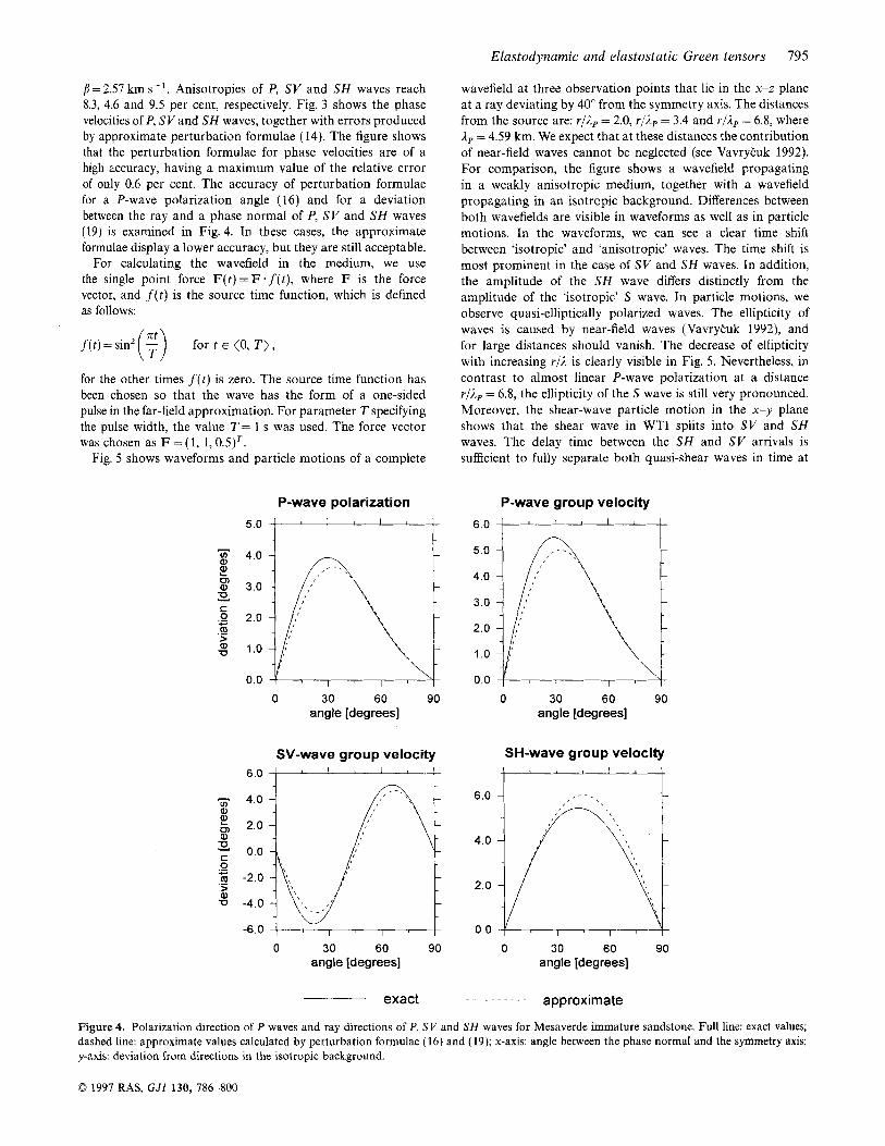
j = 2 . 5 7 km s-’. Anisotropies of P, SV and S H waves reach 8.3, 4.6 and 9.5 per cent, respectively. Fig. 3 shows the phase velocities of P, SV and SH waves, together with errors produced by approximate perturbation formulae (14). The figure shows that the perturbation formulae for phase velocities are of a high xcuracy, having a maximum value of the relative error of only 0.6 per cent. The accuracy of perturbation formulae for a P-wave polarization angle (16) and for a deviation between the ray and a phase normal of P, SV and SH waves (19) is examined in Fig. 4. In these cases, the approximate formulae display a lower accuracy, but they are still acceptable.

For calculating the wavefield in the medium, we use the single point force F(t) = F - f ( t ) , where F is the force vector, and f(t) is the source time function, which is defined as follows:

for the other times f( t ) is zero. The source time function has been chosen so that the wave has the form of a one-sided pulse in the far-field approximation. For parameter T specifying the pulse width, the value T = 1 s was used. The force vector was chosen as F = (1, 1, 0.5)T.

Fig. 5 shows waveforms and particle motions of a complete

- In a,

0) a,

C 0 m > a, U

E E ._ - .-

C 0 m > a, U

.- c

.-

P-wave polarization 5.0

4.0

3.0

2.0

1 .o

0.0

wavefield at three observation points that lie in the x-z plane at a ray deviating by 40” from the symmetry axis. The distances from the source are: r l l , = 2.0, r/& = 3.4 and r/& = 6.8, where 1, = 4.59 km. We expect that a t these distances the contribution of near-field waves cannot be neglected (see VavryEuk 1992). For comparison, the figure shows a wavefield propagating in a weakly anisotropic medium, together with a wavefield propagating in a n isotropic background. Differences between both wavefields are visible in waveforms as well as in particle motions. In the waveforms, we can see a clear time shift between ‘isotropic’ and ‘anisotropic’ waves. The time shift is most prominent in the case of SV and S H waves. In addition, the amplitude of the S H wave differs distinctly from the amplitude of the ‘isotropic’ S wave. In particle motions, we observe quasi-elliptically polarized waves. The ellipticity of waves is caused by near-field waves (VavryEuk 1992), and for large distances should vanish. The decrease of ellipticity with increasing r / l is clearly visible in Fig. 5. Nevertheless, in contrast to almost linear P-wave polarization at a distance r / l , = 6.8, the ellipticity of the S wave is still very pronounced. Moreover, the shear-wave particle motion in the x-y plane shows that the shear wave in WTI splits into SV and SH waves. The delay time between the SH and SV arrivals is sufficient to fully separate both quasi-shear waves in time at

6.0

5.0

4.0

3.0

2.0

1 .o

0.0

P-wave group velocity

t----‘----”---t

0 30 60 90 0 30 60 90 angle [degrees] angle [degrees]

SV-wave group velocity SH-wave group velocity 6.0

4.0

2.0

0.0

-2.0

-4.0

-6.0 0 30 60 90 0 30 60 90

angle [degrees] angle [degrees]

approximate ..~....... exact

Figure 4. Polarization direction of P waves and ray directions of P, SV and SH waves for Mesaverde immature sandstone. Full line: exact values; dashed line: approximate values calculated by perturbation formulae (16) and (19); x-axis: angle between the phase normal and the symmetry axis; y-axis: deviation from directions in the isotropic background.

0 1997 RAS, GJI 130, 786-800

796 V. Vauryc'uk

Waveforms

rlb = 2.0 , A! = 0.3 s

2 4 6 time [s]

Particle motions

r lb = 2.0, A t = 0.3 s

r/j = 3.4 , A! = 0.5 s

2 4 6 8 time [s]

rlb = 3.4 A t = 0.5 s

X

. . . 6 8 10 12 14

time [s]

r l h = 6 . 8 , h t = l . O s

Figure 5. Waveforms and particle motions of waves in the WTI medium (full line) and in the isotropic background (dashed line). Diagrams are shown for three receivers lying in the x-z plane at the ray deviating from the z-axis by a = 40" at distances r/A, = 2.0, 3.4 and 6.8. Parameter At represents the delay time between SH- and SV-wave arrivals.

this distance. Although the split S waves are fully separated, they still exhibit an elliptical polarization. The ellipticity of split quasi-shear waves is controlled in this case predominantly by the SV-SH coupling wave. The S-wave splitting and coupling effects are also displayed in Figs 6 and 7. Fig. 6 shows waveforms and particle motions of quasi-shear waves for the complete solution (23) and for the far-field approximation (21) at observation points situated in the x-z plane at a ray deviating by 40" from the symmetry axis. The distances from the source are: I l l S H = 8.7, rJAsH = 17 and rJlsH = 40, where ASH = 2.69 km. The corresponding separation times between the split SH and S V waves are: At = 0.75 s, At = 1.5 s and At = 3.5 s. For the first observation point the S H and SV waves are not yet fully separated, but for the other observation points they do not interfere. From the particle motions, we can see that the standard far-field approximation fails if the separation time between the SV and S H waves is not sufficiently high. Even in the case that the split S waves do not interfere, the

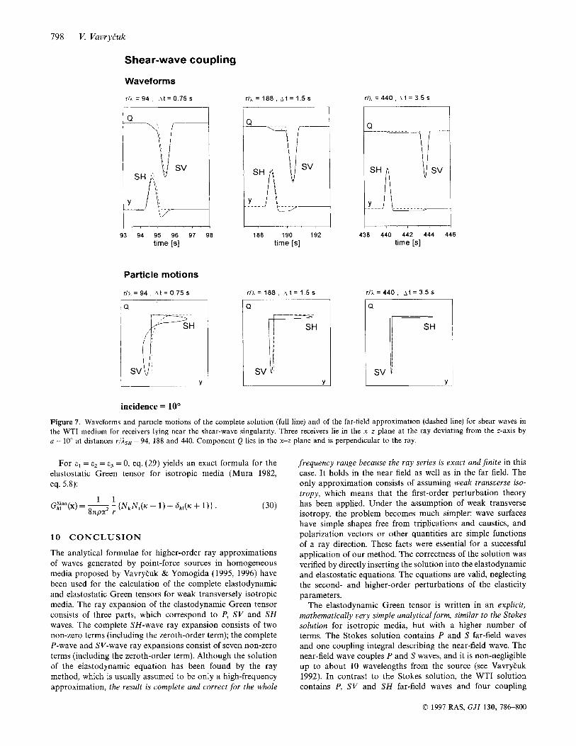
standard far-field approximation can give erroneous results. For insufficiently large separation times, we observe that the split S waves are not linearly polarized as is predicted by the far-field approximation, but they display a significant ellipticity. The ellipticity of split S waves decreases with increasing separation time. The same effect is shown in Fig. 7, but for observation points situated at a ray deviating from the symmetry axis by only 10". Since the observation points are near the S-wave singularity in this case, values of the SH- and SV-wave velocities are very close to each other, and the S waves split at very large distances from the source. The observation points for the same separation times as in Fig. 6 now have the following distances: rJAsH = 94, rJAsH = 188 and rJAsH = 440, where ASH = 2.58 km. Even at such enormously large distances the split S waves are still elliptical. It means that the shear-wave coupling is detected well and the difference between the complete solution and the standard far-field approximation is still remarkable.

0 1997 RAS, GJI 130, 786-800


Shear-wave coupling

Waveforms

rlh = 8.7 I A t = 0.75 s rlh = 17 I A t = 1.5 s

Q

7 8 9 10 1 1 time [s]

Particle motions

r / i = 8.7 ~t = 0.75 s

Q

SH

16 18 20 time [s]

Q

SV I

40 42 44 46 time Is]

r / h = 40 , A t = 3.5 S

Q

SH

SV Y

incidence = 40”

Figure 6. Waveforms and particle motions of shear waves for the complete solution (full line) and for the far-field approximation (dashed line) in the WTI medium. Three receivers lie in the x-z plane at the ray deviating from the z-axis by a = 40” at distances r/ASH = 8.7, 17 and 40. Component Q lies in the x-z plane and is perpendicular to the ray.

9 ELASTOSTATIC GREEN TENSOR

Convolving the elastodynamic Green tensor Gkl(x, t ) with the unit constant in time we obtain the elastostatic Green tensor GI (4:

m

G;i(X) = Gk,(X, t )*1 Gkl(X, t ) d t , J-, where * is the time convolution operator. Using the equations

OD

6 ( t ) d t = 1,

[H( t - tsy) - H ( t - ?“)I dt = tSH - tsv ,

[ H ( t - tp) - H ( t - tsv) l tndt = 1 [(P)”+’- ( z ~ y + l l ,

Im 1-1

m 1: m n + l

( 2 8 )

and specifying tP, 7’“ and zSH by applying eq. (19, we arrive at the final form of the elastostatic Green tensor for homogeneous

WTI:

where a , , = I + 2 p = u Z , a, ,=p=p’ and ~ = a ~ , / a , , = a ’ / ~ ’ =

The correctness of the elastostatic Green tensor was verified by directly inserting ( 2 9 ) into the elastostatic equation (Mura 1982, eq. 5.2). The elastostatic Green tensor for WTI with an arbitrarily oriented symmetry axis can be obtained from eq. ( 2 9 ) by applying standard rules for a rotation of tensors.

(2 + 2P)IP.

8 1997 RAS, GJI 130, 786-800

798 V VuvryEuk

Shear-wave coupling

Waveforms

r/i, = 9 4 , \ t = 0 75 s

93 94 95 96 97 98 time [s]

Particle motions

r / ) . = 9 4 , \ t = O 7 5 s

I Q

L Y

incidence = 10"

r/j, = 188 , ~t = 1.5 s rl?, = 440 , I t = 3 5 s

188 190 192 time [s]

r lh = 180, L3 t = 1.5 s

Q

Y

438 440 442 444 446 time [s]

r l i , = 4 4 0 , A t = 3.5 s

I Q I

Figure 7. Waveforms and particle motions of the complete solution (full line) and of the far-field approximation (dashed line) for shear waves in the WTI medium for receivers lying near the shear-wave singularity. Three receivers lie in the x-z plane at the ray deviating from the z-axis by u = 10" at distances r/LsH = 94, 188 and 440. Component Q lies in the x-z plane and is perpendicular to the ray.

For E~ = E~ = c3 = 0, eq. (29) yields an exact formula for the elastostatic Green tensor for isotropic media (Mura 1982, eq. 5.8):

1 1 8npu r G?(X) = 7 - { N , N [ ( K ~ 1) + &(IC + 1)) . (30)

10 CONCLUSION

The analytical formulae for higher-order ray approximations of waves generated by point-force sources in homogeneous media proposed by VavryEuk & Yomogida (1995, 1996) have been used for the calculation of the complete elastodynamic and elastostatic Green tensors for weak transversely isotropic media. The ray expansion of the elastodynamic Green tensor consists of three parts, which correspond to P, S V and SH waves. The complete SH-wave ray expansion consists of two non-zero terms (including the zeroth-order term); the complete P-wave and SV-wave ray expansions consist of seven non-zero terms (including the zeroth-order term). Although the solution of the elastodynamic equation has been found by the ray method, which is usually assumed to be only a high-frequency approximation, the result is complete and correct for the whole

frequency range because the ray series is exact andjnite in this case. It holds in the near field as well as in the far field. The only approximation consists of assuming weak transverse isotropy, which means that the first-order perturbation theory has been applied. Under the assumption of weak transverse isotropy, the problem becomes much simpler: wave surfaces have simple shapes free from triplications and caustics, and polarization vectors or other quantities are simple functions of a ray direction. These facts were essential for a successful application of our method. The correctness of the solution was verified by directly inserting the solution into the elastodynamic and elastostatic equations. The equations are valid, neglecting the second- and higher-order perturbations of the elasticity parameters.

The elastodynamic Green tensor is written in an explicit, mathematically very simple analytical form, similar to the Stokes solution for isotropic media, but with a higher number of terms. The Stokes solution contains P and S far-field waves and one coupling integral describing the near-field wave. The near-field wave couples P and S waves, and it is non-negligible up to about 10 wavelengths from the source (see VavryEuk 1992). In contrast to the Stokes solution, the WTI solution contains P, SV and SH far-field waves and four coupling

0 1997 RAS, GJI 130, 786-800


integrals: three of them couple P and SV waves and the fourth couples SV and S H waves. The P-SV coupling waves behave similarly to the P-S coupling wave in isotropy, thus we can again call them the near-field waves. However, the SV-SH coupling wave, which is called the ‘shear-wave coupling’ or ‘quasi-shear-wave coupling’ (Chapman & Shearer 1989; Coates & Chapman 1990), behaves exceptionally and has no analogy in the Green tensor for isotropy. The shear-wave coupling can be non-negligible even at quite large distances, thus this wave cannot be classified as the near-field wave. The shear-wave coupling considerably affects waveforms and polarization of quasi-shear waves in regions, where S waves are not well separated, and in the vicinity of shear-wave singularities. Even if the split shear waves are fully separated in time and thus do not mutually interfere, the SV-SH coupling wave can cause the polarization of both split waves to be elliptical. It implies that the standard far-field approximation (or equivalently the zeroth-order ray approximation) can be applied only to regions where the separation time between the S-wave arrivals is at least several times larger than the width of the split S pulses. For some directions, this condition can be fulfilled at distances of even hundreds of wavelengths from the source.

For simplicity, we described the WTI media by two parameters of the background isotropic medium, a,, and a44, and by three anisotropy parameters, E~ and E ~ . For this parametrization, the formula for the Green tensor seems to be the simplest. We stress, however, that the formula can be rewritten without any problems for other specifications of the WTI medium. We admit that from the viewpoint of numerical errors, other parametrizations can appear to be more suitable. In particular, a careful selection of an optimum background medium can improve the accuracy of perturbation formulae considerably. We believe that a more precise formula for the elastodynamic Green tensor for WTI can also be found by considering even higher-order perturbations of elastic parameters. In that case the ray expansion of the Green tensor will be finite again, but with a higher number of non-zero terms of the ray series. Another promising approach is calculating the Green tensor for other types of weak anisotropy or even for a general weak anisotropy. Obviously, for a general weak anisotropy, such formulae will be more extensive because of the higher number of perturbation parameters.

ACKNOWLEDGMENTS

I thank V. cerveny and I. PSenEik for many valuable discussions on the subject. I am obliged to I. PSenEik for critically reading the manuscript and offering his comments. The work was partially done while the author was visiting Hiroshima University under the JSPS postdoctoral fellowship, and the International Centre for Theoretical Physics, Trieste, Italy under the G O WEST fellowship. The work was also supported by the Grant Agency of the Czech Republic, Grant No. 205/96/0968 and by Copernicus Project PL 96 30 23.

REFERENCES

Babich, V.M., 1961. Ray method for the computation of the intensity of wave fronts in an elastic inhomogeneous anisotropic medium, in Problems of the Dynamic Theory of Propagation of Seismic Waves 5, pp. 36-46, Leningrad University Press, republished in Geophys. J . fnt., 118, 379-383 (1994).

Backus, G.E., 1965. Possible forms of seismic anisotropy of the uppermost mantle under oceans, J . geophys. Res., 70, 3429-3439.

Ben-Menahem, A. & Gibson, R.L., 1995. Radiation of elastic waves from sources embedded in anisotropic inclusions, Geophys. J . fnt., 122, 249-265.

Ben-Menahem, A. & Sena, A.G., 1990. Seismic source theory in stratified anisotropic media, J. geophys. Res., 95, 15 395-15 427.

Ben-Menahem, A., Gibson, R.L. & Sena, A.G., 1991. Green’s tensor and radiation patterns of point sources in general anisotropic inhomogeneous elastic media, Geophys. J . Znt., 107, 297-308.

Buchwald, V.T., 1959. Elastic waves in anisotropic media, Proc. R . Soc. Lond., A, 253, 563-580.

Burridge, R., 1967. The singularity on the plane lids of the wave surface of elastic media with cubic symmetry, Q. J . Mech. Appl. Math., 20, 40-56.

cerveny, V., 1972. Seismic rays and ray intensities in inhomogeneous anisotropic media, Geophys. J. R . astr. Soc., 29, 1-13.

cerveni, V., 1982. Direct and inverse kinematic problem for inhomogeneous hexagonal anisotropic media-linearization approach, Contr. Geophys. fnst. Slou. Acad. Sci., 13, 127-133.

cerveny, V., Molotkov, LA. & PSenEik, I., 1977. Ray Method in Seismology, Charles University Press, Praha.

Chapman, C.H. & Shearer, P.M., 1989. Ray tracing in azimuthally anisotropic media-11. Quasi-shear wave coupling, Geophys. J.,

Christoffel, E.G., 1877. Uber die Fortpflanzung von Stossen durch elastische feste Korper, Ann. d i Mat., 8, 193-243.

Coates, R.T. & Chapman, C.H., 1990. Quasi-shear wave coupling in weakly anisotropic 3-D media, Geophys. J . Znt., 103, 301-320.

Duff, G.F.D., 1960. The Cauchy problem for elastic waves in an anisotropic medium, Phil. Trans. R. SOC. Lond., A, 252, 249-273.

Fara, V., 1989. Ray perturbation theory for heterogeneous hexagonal anisotropic media, Geophys. J . Znt., 99, 723-737.

Hearn, A.C., 1991. REDUCE 3.4. User’s Manual. RAND Corporation, Santa Monica.

Jech, J. & PSenEik, I., 1989. First-order perturbation method for anisotropic media, Geophys. J . fnt., 99, 369-376.

Kazi-Aoual, M.N., Bonnet, G. & Jouanna, P., 1988. Response of an infinite elastic transversely isotropic medium to a point force. An analytical solution in Hankel space, Geophys. J., 93, 587-590.

Kendall, J.-M., Guest, W.S. & Thomson, C.J., 1992. Ray-theory Green’s function reciprocity and ray-centred coordinates in anisotropic media, Geophys. J. Int., 108, 364-371.

Kiselev, A.P., 1994. Body waves in a weakly anisotropic medium-I. Plane waves, Geophys. J. Int.. 118, 393-400.

Kravtsov, Yu.A. & Orlov, Yu.I., 1990. Geometrical Optics of Inhomogeneous Media, Springer Verlag, Heidelberg.

Landau, L.D. & Lifshitz, E.M., 1974. Quantum Mechanics- Nonrelatiuistic Theory, Pergamon Press, Oxford.

Lighthill, M.J., 1960. Studies on magneto-hydrodynamic waves and other anoisotropic wave motions, Phil. Trans. R. Soc. Lond., A, 252, 397-430.

Madelung, E., 1964. Die Mathematischen Hilfsmittel des Physikers, Springer Verlag, Berlin.

Morse, P.M. & Feshbach, H., 1953. Methods of Theoretical Physics, McGraw-Hill, New York, NY.

Mura, T., 1982. Micromechanics of Defects in Solids, Martinus Nijhoff, London.

Nowack, R.L. & PSenEik, I., 1991. Perturbation from isotropic to anisotropic heterogeneous media in the ray approximation, Geophys. J . Znt., 106, 1-10,

Payton, R.G., 1971. Two-dimensional anisotropic elastic waves emanating from a point source, Proc. Camh. Phil. SOC., 70, 191-210.

Payton, R.G., 1977. Symmetry-axis elastic waves for transversely isotropic media, Q. Appl. Math., 35, 63-73.

Payton, R.G., 1983. Elastic Wave Propagation in Transversely Isotropic Media, Martinus Nijhoff, The Hague.

96, 65-83.

0 1997 RAS, G J f 130, 786-800

800 V. Vaurycluk

Sayers, C.M., 1994. P-wave propagation in weakly anisotropic media, Geophys. J . Int., 116, 199-805.

Stokes, G.G., 1849. On the dynamical theory of diffraction, Trans. Camb. Phil. SOC., 9, 1-62.

Thomsen, L., 1986. Weak elastic anisotropy, Geophysics, 51, 1954-1966.

Tverdokhlebov, A. & Rose, J., 1988. On Green’s function for elastic waves in anisotropic media, J. acousr. SOC. Am., 83, 118-121.

VavryEuk, V., 1992. Polarization properties of near-field waves in homogeneous isotropic and anisotropic media: numerical modelling, Geophys. X Int., 110, 180-190.

VavryEuk, V. & Yomogida, K., 1995. Multipolar elastic fields in

homogeneous isotropic media by higher-order ray approximations, Geophys. J . Int., 121, 925-932.

VavryEuk, V. & Yomogida, K., 1996. SH-wave Green tensor for homogeneous transversely isotropic media by higher-order approximations in asymptotic ray theory, Wave Motion, 23, 83-93.

Wang, C.-Y. & Achenbach, J.D., 1993. A new method to obtain 3-D Green’s function for anisotropic solids, Wave Motion, 18, 273-289.

Wang, C.-Y. & Achenbach, J.D., 1994. Elastodynamic fundamental solutions for anisotropic solids, Geophys. J . Int., 118, 384-392.

Yeatts, F.R., 1984. Elastic radiation from a point source in an anisotropic medium, Phys. Rev., B, 29, 1674-1684.

0 1997 RAS, G J I 130, 786-800

elastodynamic and elastostatic green tensors for

Documents