Electoral Accountability and Corruption:

Evidence from the Audits of Local Governments∗

Claudio Ferraz†

PUC-Rio

Frederico Finan‡

UC-Berkeley

February 2010

Abstract

We show that political institutions affect corruption levels. We use corruption audit

reports in Brazil to construct new measures of political corruption in local governments

and test whether electoral accountability affects the corruption practices of incumbent

politicians. We find significantly less corruption in municipalities where mayors can get re-

elected. Mayors with re-election incentives misappropriate 27 percent fewer resources than

mayors without re-election incentives. These effects are more pronounced among munici-

palities with less access to information and where the likelihood of judicial punishment is

lower. Overall our findings suggest that electoral rules that enhance political accountability

play a crucial role in constraining politician’s corrupt behavior.

Key words: Accountability, Corruption, Local Governments, Re-election.

JEL: D72, D78, H41,O17.

∗We are grateful to two anonymous referees, Sandra Black, David Card, Allan Drazen, Alain de Janvry,Seema Jayachandran, Joe Hotz, Philip Keefer, Maurizio Mazzocco, Ted Miguel, Enrico Moretti, Sarah Reber,James Robinson, Gerard Roland, Elisabeth Sadoulet, Helena Svaleryd, Duncan Thomas and numerous seminarparticipants for their helpful comments and suggestions. We also thank the staff at the Controladoria Geral daUniao (CGU) for information about the details of the anti-corruption program and Paula Aniceto, LeonardoCosta and Tassia Cruz for excellent research assistance. Ferraz gratefully acknowledges financial support fromCAPES-Brazil.

†Department of Economics, Pontifıcia Universidade Catolica do Rio de Janeiro, Rua Marques de Sao Vicente,225, Gavea. Rio de Janeiro, RJ, 22451-900, Brasil. Email: cferraz@econ.puc-rio.br

‡Department of Economics, 508-1 Evans Hall #3880, UC-Berkeley, Berkeley, CA 94720-3880. Email: ffi-nan@econ.berkeley.edu; and BREAD, IZA, and NBER

1 Introduction

The abuse of entrusted power by politicians through rent-seeking and corruption is a threat

to many modern democracies. Developing countries, in particular, provide seemingly endless

examples of political elites diverting funds intended for basic public services such as health,

schools, and roads for private gains.1 While the pervasive effects of corruption on economic

development have been well documented, the root causes are poorly understood.2

Variation in electoral systems is believed to explain a significant portion of the differences

in corruption practices across countries. Because voters can oust corrupt politicians from office,

electoral rules that enhance political accountability should constrain the behavior of corrupt

politicians.3 While there are convincing theoretical arguments for why political institutions

affect corruption (see for example Myerson (1993) and Persson, Roland, and Tabellini (1997)),

the empirical evidence identifying the specific electoral structures that discipline politicians’

behavior suffers from at least two important shortcomings. First, most of these studies are

based on indices that measure perceptions rather than actual political corruption. Second, many

have relied primarily on cross-country analysis, where the inability to account for the full set

of institutional arrangements that determine corruption has made results difficult to interpret

(Adsera, Boix, and Payne (2003), Kunicov and Rose-Ackerman (2005), Lederman, Loayza, and

Soares (2005), Persson, Tabellini, and Trebbi (2003)).

In this paper, we examine the effects of electoral accountability on corruption in local gov-

ernments in Brazil. We construct new and objective measures of corruption using reports from

an anti-corruption program that audits municipalities for their use of federal funds. From these

reports we estimate the share of total federal resources transferred to municipalities that is as-

sociated with fraud in the public procurement of goods and services, diversion of funds, and

over-invoicing of goods and services.4 Based on our estimates, corruption in local governments

is responsible for losses of approximately US $550 million per year. Thus, corruption at the local

level, as in many other countries, has become an overarching concern (Rose-Ackerman 1999).

With estimates for corruption at the municipal level, we compare mayors serving in a first

term to mayors in their second term (who face a term-limit) to identify the effects of re-election

incentives. Our identification uses variation only from municipalities audited at the same time

and in the same state, while controlling for a full set of mayor and municipal characteristics.

Also, by estimating the effects of re-election incentives on political corruption at a sub-national

1See for example Di Tella and Schargrodsky (2003), Olken (2007), Reinikka and Svensson (2004)2See Knack and Keefer (1995), Mauro (1995), Bertrand et al. (2007) for studies examining the impacts of

corruption.3Despite a general perception that political corruption is harmful, some voters may still be willing to vote for

corrupt politicians in exchange for particularistic goods or based on ideological or ethnic preferences.4Although Ferraz and Finan (2008) use the same audit reports, both the data and the sample differ in two

important ways. First, here we only use municipalities that were audited prior to the 2004 municipal elections.Second, the measures constructed for this analysis are more comprehensive and extensive.

1

level, we keep constant the macro-level institutions, both formal and informal, whose differences

plague most cross-country analysis.

We find that mayors with re-election incentives are significantly less corrupt than mayors

without re-election incentives. In municipalities where mayors are in their first term, the share

of stolen resources is, on average, 27 percent lower than in municipalities with second-term

mayors. The results are robust to various specifications and estimation strategies, as well as

to alternative measures of corruption. Considering that municipalities receive, on average, 2

million dollars of federal transfers, lame-duck mayors steal approximately US$55,000 more than

first-term mayors. Assuming that in the absence of re-election incentives first-term mayors

would behave as second-term mayors, re-election incentives reduce corruption by US$160 million

throughout Brazil. This is almost half of what the federal government spent in 2002 on the Bolsa

Escola conditional cash transfer program - its largest social program providing stipends to over

4.8 million families all throughout Brazil. We also find that the effects of re-election incentives

vary considerably according to differences in the local institutional settings that govern either

the provision of information or the potential punishment corrupt politicians might suffer. For

instance, among municipalities with the presence of local media or local public prosecutors, we

find little differential effect between first and second-term mayors. Conversely, for the munic-

ipalities without local media, re-election incentives reduce political corruption by 9 percentage

points. The effects of re-election incentives are also more pronounced in municipalities where

the elections were competitive suggesting that first-term mayors with an electoral advantage can

afford to be more corrupt.

While our results are consistent with a model of electoral accountability, these findings also

have alternative interpretations. First, our results may simply reflect differences in unobserved

characteristics of the municipality that determine both reelection and corruption. To address

this concern, we demonstrate that our results are robust to a regression discontinuity approach

that compares municipalities where incumbent mayors barely won reelection in 2000 (and thus

served as a second-term mayor from 2001-2004) to municipalities where the incumbent barely lost

the election and thus was replaced by a new mayor (who then served as a first-term mayor from

2001-2004). Second, an obvious difference between first and second-term mayors is that second-

term mayors have been re-elected. If elections serve to select the most able politicians and ability

and corruption are positively correlated, then our results overestimate the effects of reelection

incentives. To test for this possibility, we compare second-term mayors with the set of first-term

mayors who are re-elected in the subsequent election, and are thus potentially as politically able

as second-term mayors. Even under this comparison, our results remain unchanged. Finally, our

results are also consistent with a simple model in which politicians learn to be corrupt over time.

Although we cannot necessarily reject this hypothesis given the data, we do provide evidence

that these differences in corruption levels cannot be entirely explained by learning. First, our

2

results are robust when comparing second-term mayors with first-term mayor that have the

same amount of political experience. Moreover, the fact that we observe important differences

depending on presence of media or the level of political competition is difficult to reconcile with

a model of pure learning.

In addition to these robustness tests, we also present two specification checks of the theory.

First, we construct a measure of violations that include less visible forms of corruption and

mismanagement. Since voters are less aware of these violations, re-election incentives should

not affect as directly this form of bad governance. We find that our data support this hy-

pothesis. Second, mayors who face the possibility of re-election should not only refrain from

rent-extraction, but may also try to procure additional funds through matching grants. We find

that mayors with re-election incentives are much more likely to attract federal funding for public

works than second term mayors, and this difference increases as the elections approach.

Our findings lend empirical support for political agency models of Barro (1970), Ferejohn

(1986) and Banks and Sundaram (1993), which highlight the importance of elections as a dis-

ciplining device.5 In this respect, our results are consistent with a growing empirical literature

documenting how electoral accountability, and term limits in particular, influences political be-

havior. Besley and Case (1995) show that term limits affect the fiscal policy of U.S. governors,

while List and Sturm (2006) provide evidence that they even influence secondary policies, such

as environmental policy. Alt, de Mesquita, and Rose (2009) also find that term limits affect the

expected quality of incumbents.6 Our paper contributes to this literature. By using objective

measures of corruption and exploiting within country variation in re-election incentives, we pro-

vide to our knowledge the first test of how electoral accountability affects political corruption.

Our findings also complement Ferraz and Finan (2008) who show that voters punish corrupt

politicians when information about corruption practices are publicized. Together, these results

suggest that electoral accountability acts as a powerful mechanism to align politicians’ actions

with voters’ preferences.

The remainder of the paper is organized as follows. Section 2 presents a theoretical framework

that links corruption to re-election incentives. It is within this context that we interpret our

empirical results. Section 3 provides some basic background information on corruption in Brazil,

and section 4 describes the data and how we construct our measures of corruption. Our empirical

strategy is discussed in section 5. The results are presented in section 6, followed by tests of

alternative explanations in section 7. Section 8 concludes the paper.

5See Persson and Tabellini (2000) and Besley (2006) for excellent reviews of political agency models.6While these studies have focused on the U.S. governors, a related literature has investigated the effects of

term limits in U.S. state legislatures. The evidence using the introduction of legislative term-limits has beenmore mixed, and depends on the measure of behavior that is analyzed (Kurtz, Cain, and Niemi 2007). Diermeier,Keane, and Merlo (2005) estimate a structural model of the behavior of members of the U.S. Congress, andsimulate the effects of imposing term limits. They find that term limits substantially increase early voluntaryexit from the House.

3

2 Theoretical Framework

In this section, we present a simple model to help interpret our empirical findings. We utilize

the political agency framework of Besley (2006), whereby voters decide whether to re-elect an

incumbent, but are unable to observe either his type or actions. In a world of corrupt and

non-corrupt politicians, a corrupt mayor who faces the possibility of re-election can exploit

this information asymmetry to increase re-election chances by refraining from rent-seeking and

behaving as a non-corrupt mayor. According to this standard model, mayors who face re-election

incentives will on average be less corrupt than mayors who do not.7

A simple agency model

Consider a two-period model with two types of politicians: a non-corrupt politician nc and

a corrupt politician c. Let π denote the proportion of non-corrupt politicians in the pool of

potential candidates. In each period, the elected politician sets a state-dependent policy et(st, i),

where i ∈ {c, nc} is the type of politician and st ∈ {0, 1} is the state of the world at time t. Each

state occurs with equal probability and is only observed by the incumbent politician.

Given the choice of policy, voters receive a payoff of V if et = st and zero otherwise. Non-

corrupt politicians set policy to maximize voters’ objectives, whereas corrupt politicians receive

a private benefit rt for setting et 6= st. The private benefit is randomly drawn each period from a

distribution G(r) with mean µ and finite support [0, R]. The model assumes that R > δ(µ + E)

where δ is a common discount factor less than one and E denotes ego-rents that politicians enjoy

from holding office.

The timing of this game is as follows. A politician is elected at the beginning of each period,

after which nature reveals to the incumbent the state of the world. If newly elected, nature also

reveals his type. Corrupt incumbents then receive a random draw from the distribution G(r)

of private benefits. After policy is set, voters observe their payoffs and then decide whether or

not to re-elect the incumbent or select a challenger who has been drawn at random from the

pool of potential politicians. After elections are held, the corrupt politicians receive another

independent draw r2 from the distribution G(r). Period 2 actions then follow and payoffs are

realized.

The perfect Bayesian Nash equilibrium of this game requires that each politician behaves

optimally in each period, given the decision rule of the voters. Because the game ends in period

2, absent re-election incentives, each politician sets his preferred policy. Non-corrupt incumbents

will set e2(s, nc) = s2, and corrupt incumbents will set e2(s, c) = 1−s2 to receive r2. Since voters

7Campante, Chor, and Do (2009) presents an alternative model where corruption depends on politician’sstability. Politicians facing more uncertainty about re-election (a shorter horizon) will extract more rents frompower.

4

are better off with non-corrupt incumbents in period 2, they maximize the likelihood that a non-

corrupt politician is elected to the second period.

The equilibrium in period 1 is much more intriguing. While non-corrupt incumbents will

still behave in accordance with voters’ objectives, corrupt politicians face a tradeoff. Because

the probability that a politician is non-corrupt conditional on observing V is greater than the

proportion of non-corrupt types in the population, that is:

Pr(i = nc|V ) =Pr(V |i = nc)Pr(i = nc)

Pr(V )

=Pr(V |i = nc)Pr(i = nc)

Pr(i = nc) + Pr(i = c)Pr(r1 ≤ δ(µ + E))

=π

π + (1− π)Pr(r1 ≤ δ(µ + E))≥ π,

voters will re-elect the incumbent if V is provided. Thus, a corrupt politician can either extract

rents r1 in period 1 and forgo re-election, or alternatively behave as a non-corrupt politician to

guarantee re-election and reap the benefits of a second term.

Given this tradeoff, the probability that a corrupt politician provide voters with a positive

payoff in period 1 is simply Pr(r1 ≤ δ(µ + E)): the probability that r1 is less than the present

value of expected future benefits from holding office in period 2. Based on the distributional

assumptions of r1, this probability, which we denote as λ, is equal to G(δ(µ + E)).

Besley (2006) shows that in equilibrium non-corrupt politicians always set et = st. Corrupt

politicians choose e2 = (1−s2) in period 2, and e1 = s1 in period 1, provided they earn sufficiently

small rents. All politicians who choose e1 = s1 will get re-elected. In equilibrium, if the ratio of

disciplined politicians to non-disciplined politicians is larger than the share of non-corrupt types,

i.e. λ1−λ

≥ π, then rent extraction will on average be higher in the second period than in the

first period, that is,8

(1− π)(1− λ)

∫ R

r1≥δ(µ+E)

rdG(r) ≤ (1− π)λ

∫ R

0

rdG(r) + (1− π)(1− λ)(1− π)

∫ R

0

rdG(r).

The intuition for this result is simple. When faced with the possibility of re-election, corrupt

politicians have the incentive to reduce rent extraction and provide more public goods. Assuming

the disciplining effect λ is sufficiently large, rents will on average be higher in the second period,

relative to the first period. We take this main testable prediction to the data by comparing the

corruption levels of first-term mayors who face the possibility of re-election to the corruption

levels of second-term mayors who are no longer eligible for re-election.

8The condition that λ1−λ ≥ π is sufficient but not necessary for rents to be higher in the second period. Rents

are higher in the second period if the following inequality holds: π∫ R

r1≥δ(µ+E)rdG(r) < λ

1−λ

∫ R

r1≥δ(µ+E)rdG(r) +

(λ + (1− λ)(1− π))∫ r1≤δ(µ+E)

0rdG(r).

5

While our model predicts that second term mayors will be more corrupt than first term

mayors, an alternative model in which mayors learn to be more corrupt over time would also

provide the same prediction even in the absence of re-election incentives. There are, however, two

additional implications that come out of a model of electoral accountability which are not present

in a model based purely on learning. First, the effects of electoral accountability on corruption

should depend on institutional features of the municipality that strengthen the incentives for

first-term mayors to reduce corruption such as the amount of information available to voters

and the competitiveness of local elections. This is unlikely to be the case in a standard model

of learning. Second, implicit in our model of re-election incentives is the assumption that voters

can infer a mayor’s level of corruption ether by direct observation or indirectly through the lack

of public goods provision. While some acts of corruption are quite visible to the public, mayors

also commit other types of violations that either voters care less about or are harder to detect

in the absence of a formal audit. Because these types of violations may not enter into citizen’s

calculus when voting, we should not expect to see a difference in their levels between first and

second-term mayors. In contrast, a model of learning would predict differences in both non-

visible and visible forms of corruption. Given the richness of our data, we are able to test these

additional implications of the model.

3 Institutional Background

Brazil introduced several institutional changes that facilitate the test of whether electoral ac-

countability affects political corruption. Figure 1 presents a timeline of these events. First,

re-election incentives were introduced in 1997 through a constitutional amendment that enabled

mayors to run for a second consecutive term in 2000 elections. Second, in 2003 the Contro-

ladoria Geral da Uniao (CGU) introduced an ambitious anti-corruption program that audits

municipalities for their use of federal funds. These audit reports provide objective measures of

corruption at the municipal level for the 2001-2004 electoral term.9 These data combined with

the constitutional amendment allow us to compare the corruption levels between municipalities

where mayors are in their first term to those where mayors are in their second term.

3.1 Brazilian mayors and their political horizons

Brazil is one of the most decentralized countries in the world. Local governments receive, on

average, $35 billion per year from the federal government to provide a significant share of public

services in the areas of education, health, transportation, and local infrastructure. Despite some

constitutional mandates that allocate portions of the budget to certain sectors, the mayor in

9Municipal elections are held countrywide at the end of the year. The new administration begins in Januaryof the following year.

6

conjunction with local legislators decide how to spend these resources. Each year the mayor

proposes a detailed budget, itemizing spending on all programs and public work projects. The

local legislature analyzes the budget proposal and then returns it to the mayor with or without

line-items vetoes. Upon receiving the revised budget, the mayor then decides how much to

spend on all of the approved items. With the large influx of resources to municipalities, local

politicians, and particularly mayors, are important political figures both at the local and in some

cases the national level.

Given these potential benefits from office, it is not surprising that over 73 percent of mayors

run for re-election. But that only 40 percent of mayors have been re-elected since the introduction

of a second consecutive term is surprising, especially compared to the large incumbency effects

that exist in U.S.10 Because re-election is not guaranteed, mayors who face the possibility of

re-election have a strong incentive to perform well in office.

Although mayors can only hold office for two consecutive terms, they do have the possibility

of returning after a one-term hiatus. This naturally begs the question of whether or not term-

limits should affect a mayor’s political horizon. In practice, despite the fact that second-term

mayors can return to office, few actually do. Among the mayors who were in their second term

during 2001-2004, only 12 percent were reelected in 2008. Moreover, only 9 percent even run for

higher offices (i.e. state or national congress, senate, or governor). Thus given the low probability

of returning to political office in the future, it is reasonable to expect the average second-term

mayor to behave as if he is serving his last term. Even if this was not the case and term-limits do

not properly capture a politician’s political horizon, the finding that first-term mayors behave

differently than second-term mayors would simply imply that we are underestimating the true

effects of re-election incentives.

3.2 Corruption Schemes in Brazil’s Municipalities

Frauds in the procurement of goods and services, diversion of funds, and over-invoicing of goods

and services are among the most common ways local politicians find to appropriate resources.

Other common irregularities include incomplete public works (paid for but unfinished); the use

of fake receipts and phantom firms (i.e. firms that only exist on paper).

Some examples are useful to illustrate these corruption technologies. A common scheme used

to divert public resources in the municipalities of El Dorado dos Carajes and Porto Seguro, for

example, include the creation of phantom firms, simulation of the call for bids, and kickbacks to

government officials.11 In other contracts, although existing firms did win the bids, none of them

10Other developing countries, such as India, do display small or even negative incumbency effects (Linden2004).

11These descriptions are based on several CGU reports and press releases available at:www.presidencia.gov.br/cgu.

7

were even aware that they had participated in the bidding process. The local administration

used the names of these firms in fake receipts to appropriate resources for public goods that were

never provided.

Another irregular practice, common in several municipalities, is a non-competitive procure-

ment process. While Brazilian law requires at least three firms to participate in any call-for-bids

involving projects in excess of $30,000 per year, the municipality of Itapetinga in the state of

Bahia, for example, highlights one of the many ways local politicians have manipulated the

process. In 2002 and 2003, the federal government transferred to Itapetinga $110,000 for the

purchase of school lunches. In 12 out of the 16 calls for bids, only one bid was ever supplied. It

was later discovered that each call for bids was posted only one hour prior to its deadline, and

not surprisingly only a firm owned by the mayor’s brother posted within the time limit. This

same scheme was uncovered for other social programs in the areas of education and health.

Mayors also divert funds intended for education and health projects towards the purchase of

cars, fuel, apartments, or payment of their friends’ salaries. In some cases, the mayor himself

is a direct beneficiary. For example, in Paranhos, Mato Grosso do Sul, $69,838 was paid to

implement a rural electrification project. As it turns out, one of the farms benefitted by the

project was owned by the mayor.

3.3 Brazil’s Anti-Corruption Audit Program

In May 2003 the government of Luiz Inacio Lula da Silva started an unprecedented anti-

corruption program based on the random auditing of municipal government’s expenditures.

The program, which is implemented through the Controladoria Geral da Uniao (CGU), aims

to discourage misuse of public funds among public administrators and fostering civil society

participation in the control of public expenditures.

The program started with the audit of 26 randomly selected municipalities, one in each state

of Brazil. It has since expanded to auditing 50 and later 60 municipalities per lottery, from a

sample of all Brazilian municipalities with less than 450,000 inhabitants.12 The lotteries, which

are held on a monthly basis at the Caixa Economica Federal in Brasilia, are drawn in conjunction

with the national lotteries. To assure a fair and transparent process, representatives of the press,

political parties, and members of the civil society are all invited to witness the lottery.

Once a municipality is chosen, the CGU gathers information on all federal funds transferred

to the municipal government from 2001 onwards. Approximately 10 to 15 CGU auditors are then

sent to the municipality to examine accounts and documents, to inspect for the existence and

quality of public work construction, and delivery of public services. Auditors also meet members

of the local community, as well as municipal councils in order to get direct complaints about any

12This excludes approximately 8 percent of Brazil’s 5500 municipalities, comprising mostly of the state capitalsand coastal cities.

8

malfeasance.13 After approximately one week of inspections, a detailed report describing all the

irregularities found is submitted to the central CGU office in Brasilia. The reports are then sent

to the Tribunal de Contas da Uniao (TCU), to public prosecutors and to the legislative branch

of the municipality. For each municipality audited, a summary of the main findings is posted

on the internet and disclosed to media sources. It is from these reports that we construct an

objective measure of corruption.

4 Data

This section describes how we constructed our measures of corruption and mismanagement. We

then present summary statistics of the variables used in the analysis.

4.1 Measuring Corruption from the Audit Reports

As with any illegal activity, obtaining data on corruption is a difficult task. Several empirical

studies that focus on illegal behavior have used indirect evidence to analyze its determinants

and consequences (see for example Duggan and Levitt (2002); Fisman (2002); Fisman and Wei

(2004), Bandiera, Prat, and Valletti (2009)). A growing body of literature, however, has tried to

assess corruption more directly by focusing on two forms: bribery of public officials and the theft

of public resources (Svensson (2003); Di Tella and Schargrodsky (2003); Reinikka and Svensson

(2004); Olken (2007)).

Our approach, although related to the studies cited above, uses a methodology made possible

by the availability of audit reports from Brazil’s anti-corruption program. Each audit report

contains the total amount of federal funds transferred to the municipal administration and the

amount audited, as well as an itemized list describing each irregularity found by the auditors

and, in most cases, the amount of funds involved. Audit reports were available in the beginning

of 2004 for 496 municipalities randomly selected across the first 11 lotteries of the anti-corruption

program.14

Although local corruption in Brazil assumes a variety of forms, most corruption schemes in

local governments are associated with three types of violations: 1) fraud in the procurement

of public goods and services; 2) diversion of public funds for private gain; 3) over-invoicing of

goods and services. Thus, for coding purposes, we define as political corruption any irregularity

13These auditors are hired based on a public examination, and prior to visiting the municipality receive extensivetraining on the specificities of the sampled municipality. Also, there is a supervisor for each team of auditors.

14Only 26 municipalities were selected in the first lottery. From lottery two to lottery nine, 50 municipalitieswere chosen in each. Starting on the tenth lottery in May of 2004, the CGU increased the number of municipalitieschosen to 60. In our estimation sample, we lose 20 municipalities because of missing values for the covariates.To including these municipalities does not affect our estimates of the unadjusted relationship between corruptionand re-election incentives.

9

associated with one of these three non-mutually exclusive categories. Specifically, we classify

diversion of resources as any irregularity involving the embezzlement of public funds. This

typically occurs in two situations: 1) federally-transferred resources simply “disappear” from

municipal bank accounts; and 2) the municipality claimed to have purchased goods and services

that were never provided, which is determined when there is no proof of purchase and community

members confirm that the goods were in fact not delivered. We classify over-invoicing as any

irregularity in which auditors determined that the goods and services were purchased at a value

above market price. We classify the irregularity as an irregular public procurement when there

is an illegal call-for-bids where the contract was awarded to a ”friendly firm” and the public

good was not provided. These firms are usually connected directly to the mayor and/or his

family or do not even physically exist. Often, corruption involving illegal public procurements

include any combination of: i) use of non-existing firms in the bidding process; ii) use of fake

receipts to pay for goods and services; iii) over-invoicing of prices to increase the amount paid

for the goods and services. These practices are not only the most common ways by which local

politicians divert public resources, but in many instances represent complementary technologies

(see Trevisan et al. (2004)).15

We read each audit report and categorize the irregularities listed by the auditors into one of

the several categories of corruption listed above.16 Based on the coding of the reports, we define

as our principal measure of corruption the total amount of resources related to corrupt activities,

expressed as a share of the total amount of resources audited. While this is our preferred measure,

we also report two additional indicators of corruption: the number of irregularities related to

corruption and the share of service items associated with corruption, which simply divides the

number of irregularities related to corruption by the number of service items audited.

There are at least two reasons why we calculate these additional measures. First, although

highly correlated with our main measure, these other indicators help to distinguish whether

second-term mayors also engage in more corrupt transactions. Second, in coding the amount

of stolen resources, a dollar amount was not available for all listed irregularities. While coding

these cases as zero underestimates the amount of corruption, this could create a bias for testing

re-election incentives if the cases occurred disproportionately more for first-term mayors. By

using additional measures we include these irregularities and thus avoid the potential bias.17

The corruption measures used in this analysis are different than the indicator used in Ferraz

15To give a better sense of the irregularities found and the procedure used to code corruption, we present inthe appendix some specific examples from the audit reports.

16We also used two independent research assistants to code the reports in order to provide a check on ourcoding.

17Approximately 89 percent of the incidences of illegal procurement practices and funds diversion have a valuereported by the auditors. Because the proportion of irregularities with no value listed is 4 percentage pointshigher for second-term mayors (although not statistically significant), if anything, we are underestimating theeffect of re-election incentives on the share of total resources associated with corruption.

10

and Finan (2008), even though these data come from the same policy experiment. In Ferraz

and Finan (2008), we construct a measure that captured the information that voters received

based on an extensive summary of the audit reports that the CGU provided to various media

sources and the municipality. The purpose of the measures used in this analysis is to have a more

comprehensive and complete measure of the corruption that occurred from 2001-2003. Hence,

we complement the information available in the audit reports posted on the internet with more

detailed audit reports provided by the CGU office.

As described above, our corruption measure captures the more blatant acts of corruption.

But mayors commit other violations that are either harder to detect or that voters care less

about.18 To measure these types of non-visible violations, we create an index of mismanagement

where we count the number of violations and divide it by the number of service items audited.19

Some examples are useful to illustrate this measure. A common violation in the procurement

of public goods occurs when less than three firms bid for a public contract. This can occur

for a variety of reasons, such as, ineptitude in publicizing the call-for-bids, lack of suppliers

in the smaller municipalities, or perhaps even corruption. But in the cases where the public

good is provided we code this violation as an act of mismanagement rather than corruption

given that voters are unlikely to detect these subtler forms of fraud. Another common form of

mismanagement occurs in the misuse of resources. Some of the block grants that municipalities

receive stipulate that the resources be spent on goods in particular sectors, such as education or

health. In some municipalities, mayors will use resources intended for health and use them on

teachers’ salaries or other public goods. Again while corruption may be involved in the misuse

of these funds, these resources were not being overtly diverted for private gain. Other violations

are more standard and they include acts such as: medicines were not being properly stored, or

schools were serving lunches that were past their expiration dates, or the mayor’s office was not

keeping school attendance for children participating in a federal school program.

4.2 Summary Statistics on Corruption and Mismanagement

Summary statistics for each one of the three corruption categories and the overall corruption

indicator are displayed in Table 1. As seen in row 1, 58 percent of the municipalities have

performed an illegal procurement practice, and 54 percent of the municipalities have diverted

funds. Over-invoicing is found much less frequently, occurring in only 7 percent of our sample.

After combining these indicators, we see that 79 percent of the municipalities have had at

least one incidence of corruption and virtually every municipality has committed some act of

18In many cases, these violations constitute what Bandiera, Prat, and Valletti (2009) refer to as passive waste.19Because of the time and cost involved in coding these reports, we only construct this measure of misman-

agement for municipalities within a randomly selected subset of the lotteries. Thus, lotteries 8, 10, and 11 wererandomly excluded and we only have this measure for 366 municipalities.

11

mismanagement (99 percent). Moreover, those administrations that commit an act of corruption

average around 2.46 corrupt violations, which is 6.7 percent of the service items audited. The

average amount of resources diverted is R$327,000 per violation which represents 8 percent of

the total amount audited. In the last column of Table 1, we also see that the ratio of acts of

mismanagement to number of service items audited is 1.65.

To get a sense for how electoral accountability may affect these various irregularities, Table

2 compares these indicators between municipalities with mayors in their first-term to those that

have mayors serving in their second-term. In the first set of columns, the share of audited

resources found to be associated with corruption is 1.9 percentage points higher for second-term

mayors (significant at the 95 percent level of confidence). Second-term mayors are also more

corrupt in each one of the three individual categories of corruption (diversion of funds, illegal

procurement practices, and over-invoicing), but it is the difference in illegal procurement that

accounts for much of the difference in the aggregate measure. On average, the share of resources

that are diverted illegally in the procurement of public works is 1.7 percentage points higher

among second-term mayors than first-term mayors.

When corruption is measured as either the incidence of irregularities or the share of service

items, in columns 4-9 of Table 2, we see further evidence in support of the theoretical predictions.

Compared to first-term mayors, second-term mayors commit 0.12 and 0.27 more irregularities

in the diversion of funds and illegal procurement practices respectively, which represent 0.2 and

0.6 percentage points differences in the share of services items audited.

4.3 Municipal and Mayor Characteristics

The other data sources used in the analysis were obtained from the Brazilian Institute of Geog-

raphy and Statistics (Instituto Brasileiro de Geografia e Estatıstica (IBGE)), Tribunal Superior

Eleitoral (TSE), and Tesouro Nacional. The richness of these data allows us to control for a large

number of municipal characteristics that are likely to be correlated with corruption practices and

whose absence might otherwise confound our estimates.20

Table 3 compares differences in mean characteristics of municipalities with a first-term mayor

to municipalities with a second-term mayor. Because of the lack of an experimental design and

the need to assume selection on observable characteristics, it is important to understand if the

determinants of corruption are significantly different across the municipalities. As the table

demonstrates, there are few differences in observable characteristics between these municipali-

ties. Out of 43 variables, only 5 are significantly different at a 95 percent level of confidence.21

There is a significant difference between first and second-term mayors in our measures of electoral

performance for the 2000 municipal elections. The other significant differences across munici-

20See the data appendix for a detailed description of data sources.21We report the 19 most important variables that are later used in our specifications.

12

palities are the proportion of the population with at least a secondary school education and

the share of the population that lives in urban areas; characteristics that are fairly correlated.

In fact, the difference in the share of the urban population loses statistical significance in our

regressions once we account for the difference in secondary school attainment.

5 Empirical Strategy

Our main objective is to test whether re-election incentives affect the level of political corruption

in a municipality. As the theory presented in Section 2 predicts, mayors who face re-election

incentives should, on average, be less corrupt than those who are no longer eligible for re-election.

To estimate these effects, the ideal experiment would be to randomly assign the possibility of

re-election across municipalities and then measure the differences in corruption levels across

these two groups of municipalities among mayors in their first term of office. Unfortunately, this

experiment design does not exist and given the cross-sectional nature of our data, we instead

compare mayors in their first term, who still face re-election incentives, to second-term mayors

using the following regression:

ri = βIi + Xiϕ + Ziγ + εi, (1)

where ri is the level of corruption for municipality i, and Ii indicates whether the mayor is

in his first term. The vector Xi is a set of municipal characteristics and the vector Zi is a

set of mayor characteristics that determine the municipality’s level of corruption. The term εi

denotes unobserved (to the econometrician) municipal and mayor characteristics that determine

corruption.

In estimating Equation 1, we face two main empirical challenges. First, without random

assignment of re-election incentives, unobserved characteristics of the municipality and the mayor

that affect both re-election and local corruption (e.g. political ability and campaigning effort)

will bias a simple OLS regression. Second, even if first and second-term mayor were randomly

assigned, the finding that second-term mayors are more corrupt could be due to the fact that

they have more experience.

To illustrate these potential biases, consider a simple model that expresses the difference in

corruption level between first and second-term mayors in terms of potential outcomes. Let rDTt

be the level of rents extracted by a politician at term t in a municipality where mayors can be

re-elected to a second term, i.e. a double-term regime, DT . The simple comparison between

mayors in their first and second term is:

∆ = E[rDT2 |τ = 2]− E[rDT

1 |τ = 1]

13

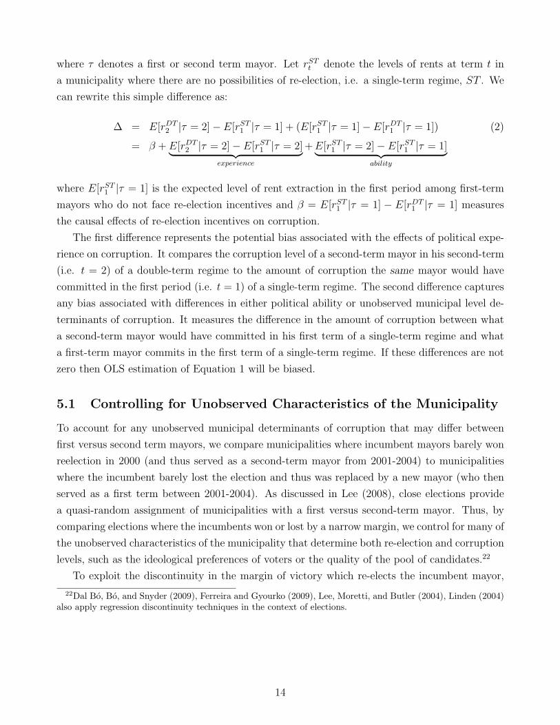
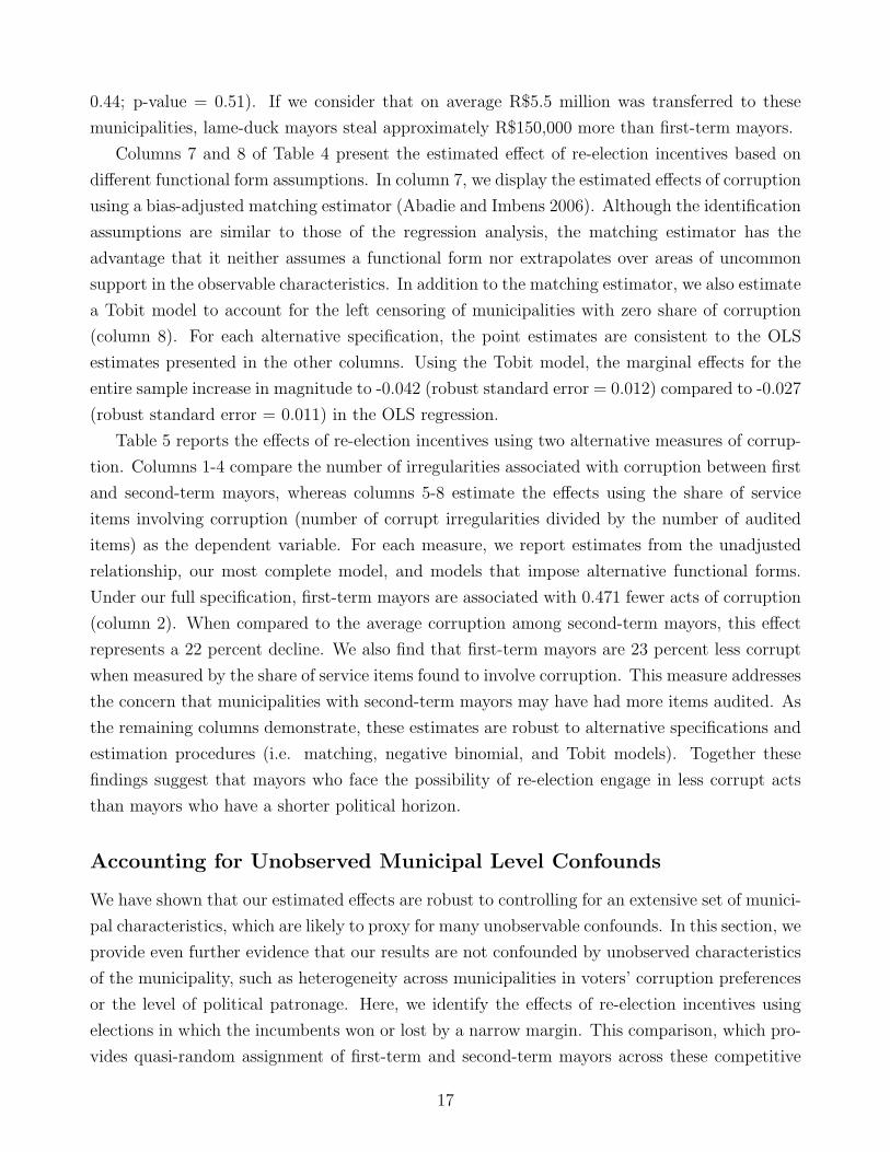
where τ denotes a first or second term mayor. Let rSTt denote the levels of rents at term t in

a municipality where there are no possibilities of re-election, i.e. a single-term regime, ST . We

can rewrite this simple difference as:

∆ = E[rDT2 |τ = 2]− E[rST

1 |τ = 1] + (E[rST1 |τ = 1]− E[rDT

1 |τ = 1]) (2)

= β + E[rDT2 |τ = 2]− E[rST

1 |τ = 2]︸ ︷︷ ︸experience

+ E[rST1 |τ = 2]− E[rST

1 |τ = 1]︸ ︷︷ ︸ability

where E[rST1 |τ = 1] is the expected level of rent extraction in the first period among first-term

mayors who do not face re-election incentives and β = E[rST1 |τ = 1] − E[rDT

1 |τ = 1] measures

the causal effects of re-election incentives on corruption.

The first difference represents the potential bias associated with the effects of political expe-

rience on corruption. It compares the corruption level of a second-term mayor in his second-term

(i.e. t = 2) of a double-term regime to the amount of corruption the same mayor would have

committed in the first period (i.e. t = 1) of a single-term regime. The second difference captures

any bias associated with differences in either political ability or unobserved municipal level de-

terminants of corruption. It measures the difference in the amount of corruption between what

a second-term mayor would have committed in his first term of a single-term regime and what

a first-term mayor commits in the first term of a single-term regime. If these differences are not

zero then OLS estimation of Equation 1 will be biased.

5.1 Controlling for Unobserved Characteristics of the Municipality

To account for any unobserved municipal determinants of corruption that may differ between

first versus second term mayors, we compare municipalities where incumbent mayors barely won

reelection in 2000 (and thus served as a second-term mayor from 2001-2004) to municipalities

where the incumbent barely lost the election and thus was replaced by a new mayor (who then

served as a first term between 2001-2004). As discussed in Lee (2008), close elections provide

a quasi-random assignment of municipalities with a first versus second-term mayor. Thus, by

comparing elections where the incumbents won or lost by a narrow margin, we control for many of

the unobserved characteristics of the municipality that determine both re-election and corruption

levels, such as the ideological preferences of voters or the quality of the pool of candidates.22

To exploit the discontinuity in the margin of victory which re-elects the incumbent mayor,

22Dal Bo, Bo, and Snyder (2009), Ferreira and Gyourko (2009), Lee, Moretti, and Butler (2004), Linden (2004)also apply regression discontinuity techniques in the context of elections.

14

we modify Equation 1 to estimate the following model:

ri = βIi + f(Wi) + Xiϕ + Ziγ + εi

Ii = 1[Wi ≥ 0]

where Wi denotes the difference in vote shares between the incumbent and the second place

candidate, and f(Wi) is a smooth continuous function of margin of victory. As is typically

the case in a regression discontinuity framework, there is a tradeoff between precision and bias,

particularly as one moves away from the discontinuity. In section 6, we present estimates that

are robust to various functional form assumptions for f(Wi).

5.2 Controlling for Political Ability and Experience

While the regression discontinuity approach does eliminate an important class of municipal-level

confounds, this identification strategy does not account for any underlying differences in the

unobserved characteristics of individual politicians. If, for instance, incumbent mayors are more

politically able than first-term mayors, then our estimates will be overestimated even when we

restrict the sample to only those municipalities with close elections. To addresses differences in

unobserved political ability, we instead compare second-term mayors with a subset of first-term

mayors that were able to get re-elected in 2004 elections. If the bias from the OLS regression

comes from unobserved political ability that positively selects more able politicians into a second-

term, this approach controls for a significant portion of this bias by comparing mayors that are

as politically able as second-term mayors.

Another empirical challenge comes from the fact that second-term mayors are by definition

more experienced then first-term mayors. Thus, if there is a learning process associated with

corruption or if it simply takes time to establish the networks that enable corrupt practices,

then the difference in corruption levels between first and second-term mayors may not only

reflect re-election incentives but also political experience.23

To account for differences in experience, we collect data on all mayors who held a political

position as either mayor or local legislator during the 1989-1992, 1993-1996, and 1997-2000

administrations. We can then compare the corruption of mayors facing a second-term with those

mayors serving on a first-term, but who have had previous political experience. If the difference

in corruption levels between first and second-term mayors is largely due to experience then we

would expect first-term mayors who had previously been in power to have similar corruption

levels to second-term mayors.24

23As long as reducing corruption increases one chances of getting re-elected then theoretically it is unlikely thatany difference between first and second-term mayors is strictly due to a learning-by-doing process.

24Underlying this comparison is the assumption that legislative experience is a good proxy for the additional

15

6 Empirical Results

This section provides evidence that municipalities where mayors face re-election incentives are

associated with significantly lower levels of corruption, as measured by the share of stolen re-

sources. These findings are robust to alternative definitions of corruption, as well as to various

specifications and estimation techniques. We also explore how re-election incentives vary with

local characteristics and find that the effects are stronger among municipalities where the cost

of rent extraction are lower and political competition is higher. All these results are consistent

with the basic predictions of a standard political agency model. We conclude this section with

additional results that address several potential threats to our identification assumptions.

Main Results on Corruption

Table 4 presents regression results from estimating several variants to Equation 1, where the

dependent variable is the share of audited resources that involved corruption. Column 1 reports

the unadjusted relationship between whether the mayor is in his first term and the share of

stolen funds. The remaining columns correspond to specifications that include additional sets of

controls. The specifications presented in columns 2-4 account for various mayors, demographic

and institutional characteristics of the municipality, whereas the specifications in columns 5 and

6 include, in addition to the other controls, indicators for when the municipality was selected for

audit (lottery intercepts) and state intercepts. The specification presented in column 6, where

re-election incentives are identified from only within state and lottery variation, accounts for any

state-specific or lottery-specific unobservable that might have affected political corruption. It

also controls for any differences across states (and in effect across time) for how the municipalities

may have been audited.

From the bivariate relationship in column 1, we see that first-term mayors are associated with

a 1.9 percentage point decrease in corruption. At an average corruption level of 0.074 among

second-term mayors, this estimate represents a 27 percent decline. As seen in the other columns,

the inclusion of additional controls has a minimal effect on the point estimate. For example

in column 6, which controls for state and lottery intercepts and various mayor and municipal

characteristics, including the amount of resources transferred to the municipality, the estimated

effect is slightly larger in magnitude (point estimate =-0.027; and robust standard error = 0.011),

but statistically indistinguishable from the estimate of the unadjusted regression (F( 1, 409) =

years of experience as a second-term mayor. This is a reasonable assumption. Local legislators influence localspending and the quality of public policy in much the same way as mayors do. For instance, legislators mustapprove and modify the municipal budget. They are also responsible for submitting bills and petitions. Whilemayors and local legislators do engage in activities that require similar knowhow, mayors do yield substantivelymore constitutional powers. But given the similarities, it is not surprising that at least 65 percent of mayorsstarted their political career as a local legislator.

16

0.44; p-value = 0.51). If we consider that on average R$5.5 million was transferred to these

municipalities, lame-duck mayors steal approximately R$150,000 more than first-term mayors.

Columns 7 and 8 of Table 4 present the estimated effect of re-election incentives based on

different functional form assumptions. In column 7, we display the estimated effects of corruption

using a bias-adjusted matching estimator (Abadie and Imbens 2006). Although the identification

assumptions are similar to those of the regression analysis, the matching estimator has the

advantage that it neither assumes a functional form nor extrapolates over areas of uncommon

support in the observable characteristics. In addition to the matching estimator, we also estimate

a Tobit model to account for the left censoring of municipalities with zero share of corruption

(column 8). For each alternative specification, the point estimates are consistent to the OLS

estimates presented in the other columns. Using the Tobit model, the marginal effects for the

entire sample increase in magnitude to -0.042 (robust standard error = 0.012) compared to -0.027

(robust standard error = 0.011) in the OLS regression.

Table 5 reports the effects of re-election incentives using two alternative measures of corrup-

tion. Columns 1-4 compare the number of irregularities associated with corruption between first

and second-term mayors, whereas columns 5-8 estimate the effects using the share of service

items involving corruption (number of corrupt irregularities divided by the number of audited

items) as the dependent variable. For each measure, we report estimates from the unadjusted

relationship, our most complete model, and models that impose alternative functional forms.

Under our full specification, first-term mayors are associated with 0.471 fewer acts of corruption

(column 2). When compared to the average corruption among second-term mayors, this effect

represents a 22 percent decline. We also find that first-term mayors are 23 percent less corrupt

when measured by the share of service items found to involve corruption. This measure addresses

the concern that municipalities with second-term mayors may have had more items audited. As

the remaining columns demonstrate, these estimates are robust to alternative specifications and

estimation procedures (i.e. matching, negative binomial, and Tobit models). Together these

findings suggest that mayors who face the possibility of re-election engage in less corrupt acts

than mayors who have a shorter political horizon.

Accounting for Unobserved Municipal Level Confounds

We have shown that our estimated effects are robust to controlling for an extensive set of munici-

pal characteristics, which are likely to proxy for many unobservable confounds. In this section, we

provide even further evidence that our results are not confounded by unobserved characteristics

of the municipality, such as heterogeneity across municipalities in voters’ corruption preferences

or the level of political patronage. Here, we identify the effects of re-election incentives using

elections in which the incumbents won or lost by a narrow margin. This comparison, which pro-

vides quasi-random assignment of first-term and second-term mayors across these competitive

17

elections, eliminates an important class of potential confounds. This identification strategy does

not however, allow us to disentangle the effects of re-election incentives from a simple model of

experience, or control for underlying differences in characteristics of politicians. We account for

these possibilities in the next set of robustness checks.

Table 6 presents the results from the regression discontinuity design for the subset of mayors

that ran for re-election. Because the sample is conditioned on the 328 incumbents who ran

for re-election in 2000, column 1 presents the OLS estimates of our full specification for this

subsample. The point estimate of -0.031 (robust standard error =0.014) is both statistically

and economically similar to the effects estimated for the overall sample. In columns 2-7 we

present results from various RDD specifications that correspond to different functional form

assumptions on the running variable – margin of victory. In columns 2-4 we estimate models

where the running variable ranges from a linear specification to a cubic specification, but restrict

the slopes to be constant. In columns 5-7, we relax the constant slope assumption using splines,

which allows for differential slopes on either side of the discontinuity.

The RDD approach yields estimates similar to those presented in Table 4. Depending on the

functional form assumptions, the coefficient on the first-term indicator varies between -0.028 and

-0.047 (robust standard errors varying from 0.019 to 0.029). For instance, allowing for a cubic

polynomial in the incumbent’s margin of victory, first-term mayors are 3.8 percentage points less

corrupt than second term mayors. The other point estimates increase in absolute magnitude as

the functional form assumption is relaxed, with the exception being in column 7. With only 328

observations, the cubic spline is estimated with less precision, but the point estimate (=-0.028) is

of the same magnitude as the other estimates. In Figure 2, we depict the main results graphically

using a third-degree polynomial fit. Similar to the regression results, there is approximately a

0.04 percentage point increase in corruption near the threshold, suggesting that second-term

mayors are more corrupt even after controlling for the potential effects of unobserved municipal

characteristics.

Our results thus far are consistent with re-election incentives reducing corrupt practices, even

after accounting for both observable and unobservable differences in municipal-characteristics

between first and second-term mayors. This does not preclude the possibility that individual

differences between first and second-term mayors are confounding the results. In the following

sections, we explore whether differences between first and second-term mayors in either political

ability or experience can explain the observed differences in corruption levels.

Accounting for Political Ability

An obvious difference between first and second-term mayors is that second-term mayors have

been re-elected. If elections serve to select the most able politicians and ability and corruption

are positively correlated, then our results overestimate the effects of reelection incentives. To

18

explore this potential bias, we can compare the corruption levels of second-term mayors to the

subset of first-term mayors who are re-elected in the subsequent elections in 2004. By selecting

on this subset of first-term mayors, we are comparing first and second-term mayors with similar

levels of innate political ability.

The results of this comparison are reported in column 1 of Table 7. The coefficient on the

first-term indicator increases in magnitude to -0.040 (robust standard error=0.013), suggesting

that second-term mayors extract a higher level of rents from office even compared to first-term

mayors of similar political ability. It is important to note however that the larger coefficient on

the first-term dummy was expected because the dissemination of the audit program decreased

the probability that corrupt mayors were re-elected (Ferraz and Finan 2008). To control for

the effects of the audits, we use an alternative strategy where we estimate the probability of re-

election using the sample of mayors that were not audited before the 2004 elections (and hence

voters did not have this information) and compute the predicted probability of a first-term mayor

getting re-elected.25 We then compare second-term mayors to the subset of first-term mayors

that were predicted to be re-elected. After controlling for the effects of the audits, the point

estimate reduces to -0.034 (robust standard error = 0.017) and is still significant at 90 percent

confidence (see column 2).

Accounting for Political Experience

Even if we account for differences in ability between first and second-term mayors, politicians

in power for a longer period of time may learn to be more corrupt over time. If this was the

case, the estimated differences in corruption between first and second-term mayors might reflect

the corruption know-how accumulated over time rather than the effects of re-election incentives.

In this section we provide evidence that, although second-term mayors have, on average, more

political experience, additional years in office cannot fully explain the difference in corruption

between first and second-term mayors.

We start by identifying the 2001-2004 mayors who were either in power during the 1989-1992,

1993-1996 administrations or served as local legislators during the 1997-2000 administration.

If the difference in corruption levels between first and second-term mayors is largely due to

experience then we would expect first-term mayors who had previously been in power to have

similar corruption levels to second-term mayors. In column 3 of Table 7, we re-estimate our

25We constructed a propensity score for whether the mayor was re-elected in the 2004 elections using variousmayor and municipal characteristics. These characteristics included: the mayor’s gender, education, marriagestatus, age, and party affiliation dummies; the municipality’s log population, population with secondary schooleducation, age of municipality, log GDP per capita, income equality, share of the legislative branch that supportsthe mayor, effective number of parties in 2000 election, an indicator for whether there is a judge in the municipality,state fixed effects. The predicted indicator is equal to one if the propensity score was greater than or equal to0.5. The estimation predicted 64 percent of the cases correctly.

19

full specification, but control for an indicator for whether the first-term mayor was in power in

one of the three previous terms. The point estimate of -0.027 (robust standard error=0.012) is

identical to the original point estimate in column 6, Table 4. In the next column, we explore

an alternative definition of political experience, in which we sum the number of years that the

mayor has been previously in office either as a mayor or legislator. As we see in column 4,

controlling for previous experience flexibly increases in magnitude our point estimate to -0.030

(robust standard error=0.012).

An alternative way to account for previous experience is to compare second-term mayors with

only first-term mayors who had been previously in power. Hence, we re-estimate the baseline

regression using all second-term mayors, but restrict first-term mayors to only those that have

been mayors before (either from 1988-1992 or 1993-1996). The coefficient on first-term, shown

in Table 7, column 5, is -0.038 (robust standard error= 0.014) further suggesting that political

experience does not determine the difference in corruption levels between first and second-term

mayors.

One potential criticism to this approach is that the political networks built by a mayor during

1992-1996 might be lost when he spends time away from office before returning in 2001. Hence,

in column 6, we re-estimate the basic model comparing second-term mayors to first-term mayors

that have had previous political experience, including experience as local legislators during the

previous term. The estimated difference in corruption between first and second-term mayors

decreases slightly to the original estimate of 2.7 percentage points (robust standard error=0.016).

Testing for Additional Implications of Re-election Incentives

Visible versus non-visible violations

As we discussed in Section 4, our corruption measures capture fairly visible forms of corruption.

Examples include such violations as the partial construction of roads and classrooms, or the

construction of dams and wells on politicians’ private farms. Other acts of corruption, while not

directly observed, could have been easily inferred by voters, such as when teachers were forced

to go on strike because the mayor had not paid their salaries in over a year or when children are

not supplied with school lunches for a school feeding program.26 It is these acts of corruption,

both directly and indirectly visible, that we would expect mayors who face re-election incentives

to avoid. Thus far, our results suggest this to be the case.

Mayors do, however, commit other types of violations which either voters care less about or

are harder to detect in the absence of a formal audit. Because these types of violations may

not enter into a voter’s calculus when voting, we should not expect to see a difference in their

levels between first and second-term mayors. To test this hypothesis, we use the audit reports

26See for instance “Desvio do FUNDEF atrasa salarios de professores”, O Globo 03/27/2005.

20

to classify a separate measure of mismanagement. Some incidences of mismanagement involve

acts of corruption that are difficult to detect, such as when public funds are not used for their

intended purposes. While others involve simple administrative violations that either voter do

not care about or do not observe, such as non-competitive bids (but where the public good was

still provided). Thus, while this measure may capture some corruption, it is unlikely that voters

have sufficient awareness of these violations to exact electoral retribution.

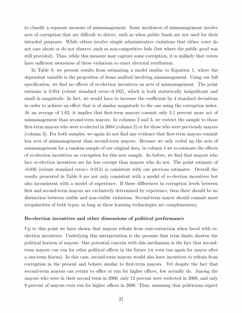
In Table 8, we present results from estimating a model similar to Equation 1, where the

dependent variable is the proportion of items audited involving mismanagement. Using our full

specification, we find no effects of re-election incentives on acts of mismanagement. The point

estimate is 0.054 (robust standard error=0.102), which is both statistically insignificant and

small in magnitude. In fact, we would have to increase the coefficient by 4 standard deviations

in order to achieve an effect that is of similar magnitude to the one using the corruption index.

At an average of 1.62, it implies that first-term mayors commit only 3.1 percent more act of

mismanagement than second-term mayors. In columns 2 and 3, we restrict the sample to those

first-term mayors who were re-elected in 2004 (column 2) or for those who were previously mayors

(column 3). For both samples, we again do not find any evidence that first-term mayors commit

less acts of mismanagement than second-term mayors. Because we only coded up the acts of

mismanagement for a random sample of our original data, in column 4 we re-estimate the effects

of re-election incentives on corruption for this new sample. As before, we find that mayors who

face re-election incentives are far less corrupt than mayors who do not. The point estimate of

-0.036 (robust standard error= 0.013) is consistent with our previous estimates. Overall the

results presented in Table 8 are not only consistent with a model of re-election incentives but

also inconsistent with a model of experience. If these differences in corruption levels between

first and second-term mayors are exclusively determined by experience, then there should be no

distinction between visible and non-visible violations. Second-term mayor should commit more

irregularities of both types, as long as these learning technologies are complementary.

Re-election incentives and other dimensions of political performance

Up to this point we have shown that mayors refrain from rent-extraction when faced with re-

election incentives. Underlying this interpretation is the premise that term limits shorten the

political horizon of mayors. One potential concern with this mechanism is the fact that second-

term mayors can run for other political offices in the future (or even run again for mayor after

a one-term hiatus). In this case, second-term mayors would also have incentives to refrain from

corruption in the present and behave similar to first-term mayors. Yet despite the fact that

second-term mayors can return to office or run for higher offices, few actually do. Among the

mayors who were in their second term in 2000, only 12 percent were reelected in 2008, and only

9 percent of mayors even run for higher offices in 2006. Thus, assuming that politicians expect

21

low probabilities of returning to office and discount future gains, it is reasonable to expect that

on average second-term mayors will act as if they face real term-limits.

Moreover, if mayors respond to re-election opportunities, then they will not only refrain

from rent extraction, but will also exert effort along other dimensions of political performance.

In this subsection, we examine whether re-election incentives affect whether mayors procure

matching grants from the central government, which is the only mechanism mayors have to

attract additional discretionary resources to their municipalities. If the political horizon of

second-term mayors is similar to those of first-term mayors then we would not expect a difference

between first and second-term mayors in the amount of grants that mayors attract.

To test this, we collect annual data on every matching grant solicited by a municipality and

the value transferred from the federal government during 2001-2004.27 These data on matching

grants are useful for two reasons. First, unlike other transfers received by the municipality, the

receipt of these funds is not formula based, but depends on the ability and effort of the mayor

to procure them. Second, in almost all cases, these contracts designate the construction of some

large public works projects, such as road construction, schools, health clinics, rural electrification,

among others. Thus, they constitute highly visible projects that can garner electoral support.

For these reasons, we would expect that, on average, mayors with re-election incentives procure

more grants than those who do not face re-election incentives.

To test the effects of re-election incentives on the receipt of matching grants, we exploit the

panel structure of the data to estimate the following model:

yit = α0 +∑

t

αt(Tt × Ii) + λt + ηi + εit (3)

where yit denotes one of three dependent variables: 1) indicator for whether the municipality

signed a matching grant in year t; 2) log value of all contracts signed in year t expressed in per

capita terms; 3) percentage of signed contracts disbursed in year t.28 The term Tt × Ii denotes

the interaction between being a first-term mayor Ii and the year of the contract; λt denotes

year effects and ηi represents municipal fixed-effects. The error term, εit, is clustered at the

municipality level.

Table 9 presents regression results from estimating variants to Equation 3. In odd columns,

we estimate the model without municipal fixed-effects (and thus included a dummy for whether

the mayor is in his first term) but control for various municipal and mayor characteristics. In

column 2 and 4, we include municipal fixed-effects and differential time trends by each of our

municipal and mayor characteristics. The coefficients presented in columns 1 and 2 reveal a

27Matching grants are contracts between the federal government and the municipality specifying each partiescontribution to the construction of a public works. However, in virtually all cases, municipalities contribute lessthan 10 percent of the expected costs.

28To avoid problems associated with ln(0), we add a 1 to the contract value before taking the log.

22

striking pattern in whether or not a municipality received a contract. During their first year

in office, first-term mayors are 5.8 percentage points less likely than second-term mayors to

attract any grants. This result is not too surprising given their lack of experience. But in

subsequent years, first term mayors become more likely to procure grants. For instance, during

the electoral year 2004, first-term mayors are 14 percentage points more likely to attract a grant

than second-term mayors (robust standard error = 0.049). Moreover, the difference between first

and second-term mayors increases as the elections approach. Although we cannot reject that

these coefficients are not statistically the same, the economic differences in magnitudes are quite

meaningful.

We also observe a similar pattern in columns 3 and 4, when we use the per capita value of

the contract as the dependent variable. Again, while first term mayors attract significantly less

funds during their first year in office, the difference is quickly reversed in subsequent years. Given

that the average length of a matching grant is 17 months, the electoral rewards for procuring

them can be high even in the second year of office.

Finally, in the remaining columns of Table 9 we examine whether the percentage of funds

disbursed exhibit similar pattern. Mayors who face the possibility of re-election not only have an

incentive to attract more grants, but to also sign contracts in which the funds can be disbursed

prior to the elections, so as to claim credit for the public work. In columns 5 and 6, we find

that first-term mayors receive a much higher percentage of the signed contract compared to

second-term mayors. Again, this difference increases as the elections near.

Overall the results presented in Table 9 are consistent with our findings that electoral ac-

countability reduces corruption practices. Moreover, the findings are difficult to reconcile with

an alternative model in which experience drives the differences in political performance between

first and second-term mayors. If experience was the principal mechanism, we would find a pat-

tern where either second-term mayor consistently attracted more grants over time, or where the

difference in grants attracted by first and second-term mayors decreased over time.

Local Context and Re-election Incentives

In this section we explore the extent to which the effects of re-election incentives on corruption

might vary according to local characteristics that affect electoral accountability. In order to shed

light on the empirical results, we start by discussing some natural extensions to the simple model

presented in Section 2.

The asymmetry of information between voters and politicians lies at the heart of political

agency models. Hence, factors that influence access to information may affect how re-election

incentives affect corruption. To see this in the framework proposed in Section 2, suppose that

with some probability, τ , voters observe their politician’s type after he has chosen his action, e

and before the election is held. In this case, the likelihood that a corrupt politician will pool with

23

non-corrupt politicians will depend negatively on τ , (i.e. ∂λ∂τ

where λ = G((1−τ)δ(µ+E))). Thus,

as the likelihood that a corrupt politician is detected in the first period increases (i.e. voters have

more information), a corrupt politician will be less likely to pool with non-corrupt politicians,

and hence discipline will be reduced. But as corrupt politicians become less disciplined, they are

less likely to survive into a second-period and the quality of the average politician that survives

into a second-mandate improves. Hence, the overall effect of an increase of information that

allows voters to identify politicians’ type is ambiguous– corruption will decrease in the second

period and potentially increase in the first because those corrupt mayors will now extract as much

rent as they can in the first period.29 Empirically, with a cross-section of mayors, one would

expect that the difference in corruption between first and second-term mayors to be smaller

in municipalities where there is more access to information that allows voters to uncover the

politician’s type.

To proxy for access to information, we use an indicator for the presence of local media in the

form of either a radio station or a local newspaper. Since the re-democratization of Brazil in the

early 1980s, local radio has played a central role in local politics, and has been a natural medium

for informing voters about politician behavior (Ferraz and Finan 2008). Because we want our

proxy to identify places with better access to information, we also include in our definition of

media the existence of local newspapers. Although circulation rates of Brazilian newspapers

tend to be relatively low, newspapers may offer a greater degree of investigative journalism than

that of radio stations.30

An additional source of heterogeneity stems from differences across municipalities in the

potential punishment of engaging in corruption. For instance, the probability of being prosecuted

and punished for corruption charges is likely to be higher in municipalities where the judiciary

has a public prosecutor, thus increasing the cost of engaging in corrupt activities. To capture

this feature in our framework, one could assume that corrupt mayors receive a private benefit θrt,

where θ ≤ 1 represents the cost of being corrupt. Corrupt mayors in deciding to accept the private

benefit trade off the rents in the first period r1 to the prospects of future benefits 1θδ(θµ + E).

Thus, as corruption costs increase, thus reducing the future benefits of rent extraction, politicians

will become less disciplined and the selection effect will increase. Therefore, we would expect

that in municipalities where the costs of engaging in corruption are higher, the difference in

corruption between first and second-term mayors will also be lower. To distinguish between

municipalities where the cost of engaging in corruption may be higher, we use an indicator for

29Alternatively, one could assume that rather than observe the politician’s type, we could suppose that actionsare only observed with some probability τ . The probability of a politician acting disciplined is then: λ =G(τδ(µ + E)). In this situation, increasing the probability of observing the politician’s action increases theprobability that bad types pool with good types. Thus in this model, we would expect the difference in corruptionlevels between first and second-term mayors to be higher in areas with local media.

30Our results are similar if we only use the presences of a local radio station as our proxy for access toinformation.

24

the presence of a judge, which can increase the likelihood of being prosecuted.31

Political competition may also determine how re-election incentives affect corruption. An

increase in electoral advantage will reduce the disciplining effect, as the probability of being

re-elected increases, even if the corrupt mayor does not pretend to be non-corrupt. Thus, the

difference between first and second-term mayors is less in municipalities where the elections are

less competitive.

Finally, a mayor’s political support might affect corruption choices. If the mayor has a

majority in the local legislature, he will be able to pass legislations, increase public employment

and adopt other strategies that increase his re-election chances. Everything else constant, he

can be less disciplined and still get reelected into a second-term. Thus, we expect the difference

in corruption between first and second term mayors to decrease as the support in the local

legislature increase.

In Table 10, we see that the presence of public prosecutors or a local media reduces the corrup-

tion differential between first-term and second-term mayors. Among municipalities with public

prosecutors, there is only a small difference in corruption levels between first and second-term

mayors (column 1), and in municipalities with local media the difference is only 1.4 percentage

points (column 2). In contrast, among municipalities where there does not exist any local media,

second-term mayors are almost 10 percentage points (robust standard error=0.03) more corrupt

than first-term mayors, which represents an average R$525,000.

In column 2, we also find that the presence of local media has a direct effect on corruption

levels. In municipalities with a second-term mayor, the existence of media reduces corruption by

5.3 percentage points. But in municipalities with a first-term mayor, corruption is 3.3 percentage

points higher in areas with media relative to those without. This is again consistent with the

theory. Because media increases the probability that the politician’s type is revealed, we expect

less discipline among first term mayors (and thus higher corruption levels) but less corruption in

municipalities with second-term mayors due to the positive selection effects. The direct effects

of having a local prosecutor are similar to those of media, but are not statistically significant.

Columns 3 and 4 report how the second-term effect varies with the degree of political com-

petition, as measured by the proportion of the local council that is from the same party as the

mayor (column 3) and a political Herfindahl index in the previous election (column 4).32 As

reported in column 3, political competition increases the difference in corruption levels between

first and second-term mayors. When only 9 percent of the legislative council is from the same

political party as the mayor (5th percentile of the distribution), there an 8.8 percentage point

difference between first and second-term mayors. Whereas, when the political support of the

31In Brazil, the presence of a judge depends on whether the municipality is a judiciary district (comarca),which in turn depends on local characteristics such as population, local revenues and the number of judiciaryprocesses.

32The Herfindahl index is computed by dividing one by the effective number of political parties.

25

incumbent mayor represents 55 percent of the legislative branch, then there is no difference in

corruption levels between first and second-term mayors. The results reported in Column 4 tell

a similar story. For instance, among municipalities where the Hefindahl index was 0.08 (the

1st percentile of the distribution), first-term mayors are 3.9 percentage points less corrupt that

second-term mayors. In contrast, when elections are less competitive at 0.528 (the 99 percentile

of the distribution), the difference in corruption levels between first and second-term mayors is

-0.007. In effect, the results presented in columns (3) and (4) suggest that municipalities char-

acterized by low competition exhibit no differential effect in rent-extraction between first and

second-term mayors. First-term mayors with an extreme electoral advantage can afford to be as

corrupt as a lame-duck mayor since his re-election is practically guaranteed.

In sum, the effects reported in Table 10 are consistent with a model where incumbent politi-

cians are responsive to re-election incentives. These interaction effects also provide even further

evidence that a model of experience cannot be the principal mechanism explaining the difference

in corruption levels between first and second-term mayors. For instance, in a simple learning

model, we would not observe first-term mayors behaving as second-term mayors in municipalities

where the political competition is low.

7 Testing for Alternative Explanations

Our analysis shows that mayors who can be held accountable at the polls will engage in less

corruption. First-term mayors steal 27 percent less resources than second-term mayors even

when accounting for potential biases in political ability and experience.

An obvious concern in interpreting this finding is that it may simply reflect corruption on

the part of the auditors. Because first-term mayors have more incentive to bribe the auditors

for a more favorable report, we could be capturing the effects of re-election incentives on bribing

rather than the effects of career concerns on actual corruption. While it is difficult to test this

hypothesis directly, we provide suggestive evidence that this is not the case. For instance, if

first-term mayors are more likely to bribe auditors, we might expect those who were audited

during the election year or affiliated with either the federal government or state government to

receive more favorable reports.

We explore these possibilities in Table 11. In columns 1-3 we regress our measure of corrup-

tion on the first-term indicator and interaction terms with variables that would suggest larger

incentives for bribing the auditors. In column 1 we test for differential auditing according to

whether the municipality was drawn to be audited during the 2004 election year. We show that

there is no difference in corruption levels between first and second-term mayors depending on

whether they were audited during the electoral year or not (coefficient= 0.001, robust standard

error=0.017). We also do not find any differential effects by whether the mayor belongs to the

26

same party of the president – the PT (Worker’s Party) – (column 2) or the state governor (col-

umn 3).33 An alternative way in which auditors may have favored first-term mayors could have

been to audit less valued projects. Although this is unlikely to explain the patterns that we find

in the main regressions, we regress the log value of projects audited on an indicator for whether

the mayor is in a first-term. As reported in column 4, we again do not find any statistically sig-

nificant difference in the amount of resources audited between first and second term-mayors. We

also do not find any differential effects depending on whether the municipality was audit during

the 2004 electoral year (column 5), whether the mayor was from the Worker’s Party (column 6),

or whether the mayor was from the same party as the governor (column 7).

In addition to the previous analysis, there are several reasons why it is unlikely that differences

in corruption between first and second-term mayors reflect corrupt auditors. First, they are

federal public employees hired based on a highly competitive public examination and high salary.

Moreover, each team of auditors reports to a regional supervisor. Therefore, not only is it hard

to cheat individually, but also the cost of getting caught is large. According to program officials,

there has never been an incidence in which auditors have even been caught receiving bribes.

Another alternative explanation for the difference in reported corruption levels is that lame

duck mayors, who are no longer accountable to voters, simply have less incentive to hide or are

less careful in their attempt to hide corruption. Although this hypothesis is in many respects

observationally equivalent to what we find, it is unlikely that this could explain the estimated

effects since this program was unexpected and the audits were based on past behavior. Moreover,

although second term mayors may not face electoral retribution, they also have an incentive to

hide corruption due to potential judiciary prosecution.

8 Conclusions

The abuse of entrusted power by democratically-elected politicians through rent-seeking and

corruption is a central issue in a large number of countries. Thus the capacity of elections to solve

the inherent agency problem between voters and elected representatives has been a central area of

research in political economy. In this paper, we examine whether electoral accountability induced

by the possibility of reelection can discipline incumbent politicians and control their rent-seeking

behavior. We provide empirical evidence that re-election incentives reduce corruption. Using a

new data set of corruption practices by local politicians in Brazil and exploiting the variation in

electoral incentives provided by term limits, we show that first-term mayors eligible for re-election

are associated with significantly less corruption than second-term mayors who face a binding

term-limit. This difference in corruption is remarkably robust to various specifications and

33Ferraz and Finan (2008) compare corruption levels using the count measure between first-term mayors thatwere audited before the election versus after the election. They do not find any evidence that corruption levelsdiffered between these two groups along various dimensions.

27

alternative interpretations such as unobserved differences in municipal characteristics, political

ability or experience between first and second-term mayors. These findings suggest that electoral

rules that enhance political accountability play a crucial role in constraining politicians even in

an institutional context where corruption is pervasive and elites dominate local politics.

We interpret our findings in the context of a simple political agency model where incumbent

mayors with electoral concerns restrain from corruption due to the possibility that voters learn

about their rent-seeking behavior and punish them at the polls. Consistent with this mechanism,

we find that the effect of electoral accountability on reducing corruption is higher in places where

the probability of corrupt practices being detected is higher (as measured by the presence of local

media and local judiciary agents). Moreover, while politicians with re-election incentives should

refrain from rent-seeking activities that voters can observe, they need not refrain from committing

irregularities that voters either cannot detect or care less about. We find that violations that

are unlikely to be uncovered by voters do not differ between first and second-term mayors.

The result that electoral accountability can reduce corruption also raises the critical question

of how to make local governments more accountable. Allowing citizens to have better information

about policy implementations and corruption practices is one possibility. In this regard, audit

policies that reveal new information about government quality can increase the probability that

bad politicians get caught. Together with the use of ”information campaigns”, it can help voters

to select better leaders. Finally, political competition and the overall improvement of the quality

of politicians, especially in local legislatures, can enhance checks and balances between executive

and legislative powers.

Finally, given our findings, it is natural to ask whether a two-term limit system is optimal to

reduce the incentives for rent-extraction. Although Smart and Sturm (2006) provide theoretical

justification for why a two-term limit regime might be optimal under some conditions, we are

unfortunately unable to test this. Unlike the variation that exists in term-limits across the U.S.,

our research design can only identify the effects of re-election incentives on corruption under a

two-term regime relative to a one-term regime. We cannot estimate for instance how politicians

would behave if they were elected for a third term or even re-elected indefinitely. Moreover,

the fact that incumbent politicians respond to electoral incentives and reduce corrupt practices

does not imply that term-limits should necessarily be abolished. In theory, term-limits can

have beneficial effects as well. Because re-election incentives can induce politicians to pander

to voters or adopt inefficient policies near elections, term limits may provide politicians with

the freedom to enact policies that are more socially optimal (Canes-Wrone, Herron, and Shotts

2001). Without term limits, entrenchment effects also become a concern. Although we suspect

that this is less likely to occur in Brazil where incumbency rates are low, entrenchment effects

can deter the entry of new leaders and reduce the overall quality of the political class in the

long-run (Dick and Jr. (1993), Buchanan and Congleton (1994)). In sum, despite the fact that

28

re-election incentives constrains corruption, further research is needed to assess whether electoral

accountability affects other aspects of governance and ultimately improves voters’ welfare.

References

Abadie, Alberto, and Guido Imbens. 2006. “Large Sample Properties of Matching Estimators

for Average Treatment Effects.” Econometrica 74 (1): 235–267.

Adsera, Alicia, Carles Boix, and Mark Payne. 2003. “Are You Being Served? Political Account-

ability and the Quality of Government.” The Journal of Law, Economics, and Organization

19, no. 2 (445-490).

Alt, James, Ethan Bueno de Mesquita, and Shanna Rose. 2009. “Accountability and Compe-

tence in Elections: Theory and Evidence from U.S. Term Limits.” Mimeo.

Bandiera, Oriana, Andrea Prat, and Tommaso Valletti. 2009. “Active and Passive Waste in

Government Spending: Evidence from a Policy Experiment.” American Economic Review

99 (4): 1278–1308 (September).

Banks, Jeffrey S., and Rangarajan K. Sundaram. 1993. “Adverse Selection and Moral Hazard in

a Repeated Elections Model.” In Political Economy: Institutions, Information, Competition,

and Representation, edited by et al W. Barnett. Cambridge and New York: Cambridge

University Press.

Barro, Robert J. 1970. “The Control of Politicians: An Economic Model.” Public Choice

14:19–42.

Bertrand, Marianne, Simeon Djankov, Rema Hanna, and Sendhil Mullainathan. 2007. “Does

Corruption Produce Unsafe Drivers?” Quarterly Journal of Economics CXXII (4): 1639–

1676 (November).

Besley, Timothy J. 2006. Principled Agents? The Political Economy of Good Government.

Oxford, UK: The Lindahl Lectures, Oxford University Press.

Besley, Timothy J., and Anne Case. 1995. “Does Electoral Accountability Affect Economic Pol-

icy Choices? Evidence from Gubernatorial Term Limits.” Quarterly Journal of Economics

110 (3): 769–798 (August).

Buchanan, James M., and Roger D. Congleton. 1994. “The Incumbency Dilemma and Rent

Extraction by Legislators.” Public Choice 79 (1-2): 47–60 (April).

Campante, Filipe R., Davin Chor, and Quoc-Anh Do. 2009. “Instability and the Incentives for

Corruption.” Economics & Politics 21 (1): 42–92 (March).

29

Canes-Wrone, Brandice, Michael C. Herron, and Kenneth W. Shotts. 2001. “Leadership and

Pandering: A Theory of Executive Policymaking.” American Journal of Political Science

45 (3): 532–550.

Dal Bo, Ernesto, Pedro Dal Bo, and Jason Snyder. 2009. “Political Dynasties.” Review of

Economic Studies 76, no. 1.

Dick, Andrew R., and John R. Lott Jr. 1993. “Reconciling Voters Behavior with Legislative

Term Limits.” Journal of Public Economics 50 (1): 1–14.

Diermeier, Daniel, Michael Keane, and Antonio Merlo. 2005. “A Political Economy Model of

Congressional Careers.” American Economic Review 95:347–373.

Di Tella, Rafael, and Ernesto Schargrodsky. 2003. “The Role of Wages and Auditing During a

Crackdown on Corruption in the City of Buenos Aires.” Journal of Law and Economics 46

(1): 269.

Duggan, Mark, and Steven D. Levitt. 2002. “Winning Isnt Everything: Corruption in Sumo

Wrestling.” American Economic Review 92 (5): 1594 605.

Ferejohn, John. 1986. “Incumbent Performance and Electoral Control.” Public Choice 50:5–25.

Ferraz, Claudio, and Frederico Finan. 2008. “Exposing Corrupt Politicians:The Effects Of

Brazils Publicly-released Audits on Electoral Outcomes.” Quarterly Journal of Economics

123 (3): 703–745 (May).

Ferreira, Fernando, and Joseph Gyourko. 2009. “Do Political Parties Matter? Evidence from

U.S. Cities.” Quarterly Journal of Economics 124 (1): 349–397.

Fisman, Raymond. 2002. “Estimating the Value of Political Connections.” American Economic

Review 91 (4): 10951102.

Fisman, Raymond, and Shang-Jin Wei. 2004. “Tax Rates and Tax Evasion: Evidence from

Missing Imports in China.” Journal of Political Economy 112:471–496.

Glaeser, Edward L., and Raven E. Saks. 2006. “Corruption in America.” Journal of Public

Economics 90:1053–1072.

Knack, Stephen, and Philip Keefer. 1995. “Institutions and Economic Performance: Cross-

Country Tests Using Alternative Institutional Measures.” Economics and Politics 7 (3):

207–227.

Kunicov, Jana, and Susan Rose-Ackerman. 2005. “Electoral Rules and Constitutional Struc-

tures as Constraints on Corruption.” British Journal of Political Science 35, no. 4 (October).

Kurtz, Karl T., Bruce Cain, and Richard G. Niemi. 2007. Institutional Change in American

Politics: The Case of Term Limits. Ann Arbor, Michigan: University of Michigan Press.

30

Lederman, Daniel, Norman Loayza, and Rodrigo Reis Soares. 2005. “Accountability and

Corruption: Political Institutions Matter.” Economics and Politics 17 (1): 1–35 (March).

Lee, David S. 2008. “Randomized Experiments from Non-random Selection in U.S. House

Elections.” Journal of Econometrics 142 (2): 675–697.

Lee, David.S., Enrico Moretti, and Matthew J. Butler. 2004. “Do Voters Affect or Elect

Policies? Evidence from the U.S. House.” Quarterly Journal of Economics 119:807–859.

Linden, Leigh L. 2004. “Are Incumbents Always Advantaged? The Preference for Non-

Incumbents in India.” Working paper.

List, John A., and Daniel M. Sturm. 2006. “How Elections Matter: Theory and Evidence from

Environmental Policy.” Quarterly Journal of Economics 121 (4): 1249–1281 (November).

Mauro, Paolo. 1995. “Corruption and Growth.” Quarterly Journal of Economics, no. 110:681–

712.

Myerson, Roger B. 1993. “Effectiveness of Electoral Systems for Reducing Government Cor-

ruption: A Game Theoretical Analysis.” Games and Economic Behavior 5:118–132.

Olken, Benjamin A. 2007. “Monitoring Corruption: Evidence from a Field Experiment in

Indonesia.” Journal of Political Economy 115, no. 2 (April).

Persson, Torsten, Gerard Roland, and Guido E. Tabellini. 1997. “Separation of Powers and

Political Accountability.” Quarterly Journal of Economics 112 (4): 1163–1202 (November).

Persson, Torsten, and Guido E. Tabellini. 2000. Political Economics: Explaining Economic

Policy. Cambridge, Massachussets: MIT Press.

Persson, Torsten, Guido E. Tabellini, and Francesco Trebbi. 2003. “Electoral Rules and Cor-

ruption.” Journal of the European Economic Association 1, no. 4 (June).

Reinikka, Ritva, and Jakob Svensson. 2004. “Local Capture: Evidence from a Central Gov-

ernment Transfer Program in Uganda.” Quaterly Journal of Economics 119 (2): 679–705

(May).

Rose-Ackerman, Susan. 1999. Corruption and Government: Causes, Consequences, and Re-

form. New York: Cambridge University Press.

Smart, Michael, and Daniel M. Sturm. 2006. “Term Limits and Electoral Accountability.”

CEPR Discussion Paper 4272, July.

Svensson, Jakob. 2003. “Who Must Pay Bribes and How Much? Evidence from a Cross-Section

of Firms.” Quarterly Journal of Economics CXVIII (February): 207–230.

Treisman, Daniel. 2000. “The causes of corruption.” Journal of Public Economics, vol. 76.

31

Trevisan, Antoninho Marmo, Antonio Chizzotti, Joao Alberto Ianhez, Jose Chizzotti, and

Josmar Verillo. 2004. O Combate a Corrupcao nas Prefeituras do Brasil. Sao Paulo, Brasil:

Atelie Editorial.

32

Appendix A: Coding the Audit Reports

This appendix explains how we used the audit reports to construct indicators of corruption.

We provide the definition used for each type of irregularity and include an illustrative example

drawn from the reports.34

Examples of Political Corruption

Health related purchases without procurement using false receipts: The ministry of Health

transferred to the municipality R$ 321,700 for the Programa de Atencao Bsica. The mu-

nicipal government used fake receipts valued at R$ 166,000 to provide proof of purchase.

Furthermore, there is no proof that the goods were purchased since there were no registered

entries of the merchandize in the stock. Also, in 2003 the municipality bought medicines

valued at R$253,300 without procurement. In 2004, the value was R$113,700, also without

procurement. We classified this violation as an incidence of irregular procurement and

diversion of public funds in the area of health. We valued this irregularity as a diversion

of R$166,000. This irregularity occurred in Capelinha, Minas Gerais, drawn by lottery

number 9.

Evidence of irregularities in well construction: The Ministry of National Integration trans-

ferred R$117,037 to the municipality for the maintenance of water infra-structure. The

working plan specified the maintenance of ten wells and four dams. None of these repairs

were made. Instead, the dam Henrique Dantas, located inside a private farm was repaired.

We classified this violation as an incidence of diversion of public funds in the area of water

and sanitation. We valued this irregularity as a diversion of R$117,037. This irregularity

occurred in Santa Cruz, Rio Grande do Norte, drawn by lottery number 9.

Over-invoice of more than R$3 million in road construction: The firm Mazda was hired,

without procurement, to build approximatly nine kilometers of a road. The cost of the

construction was estimated at R$ 1 million based on similar constructions. The receipts

presented by Mazda and paid by the government totalled R$ 5 million. No further doc-

umentation was shown by the municipal government proving the need for the additional

amount of resources. The auditors found that the firm Mazda, did not have any experi-

ence with construction and had sub-contracted the firm CTE for R$ 1.8 million to do the

construction. Hence, the project was over paid by more than R$ 3 million. As evidence

of corruption, it was late found that the firm Mazda gave an apartment for the mayor

and his family valued at R$600,000 suggesting a kickback. We classified this violation as

an incidence of over-invoice in the area of infrastructure. We valued this irregularity as a

34For access to the summary of the audit reports, see www.cgu.gov.br

33

diversion of R$3.2 million. This irregularity occurred in Sao Francisco do Conde, Bahia,

drawn by lottery number 6.

Appendix B: Data Sources

The data used in the paper comes from a variety of sources. The data is at the level of the

municipality, the lowest government unit below a state in Brazil.

Municipal demographic characteristics: The 2000 population census provides socio-economic

and demographic characteristics of municipalities. The variables we include in our analysis

are: population size, percentage of urban households, Gini coefficient and the percentage

of adults with secondary education. In addition, we also include the level of income mea-

sured by municipal GDP per capita estimated by the IBGE. These variables are important

determinants of corruption as shown by Glaeser and Saks (2006) and Treisman (2000).

Municipal institutional and public management characteristics: Our second complemen-

tary data source from IBGE is a municipality survey, Perfil dos Municıpios Brasileiros:

Gestao Publica, conducted in 1999 and 2001. The survey provides structural features of

the municipality such as the existence of local daily newspaper, radio, local public pros-

ecutors and the age of the municipality. These data also characterize various aspects of

the public administration, including the existence of laws which govern its budgetary and

planning procedures.

Election data: Results from 2000 and 2004 mayor elections are available from the Tribunal

Superior Eleitoral (TSE). These data contain vote totals for each candidate by municipal-

ity, along with various individual characteristics such as the candidate’s gender, education,

occupation, and party affiliation. We use this information to construct measures of elec-

toral performance, and to control for individual mayor characteristics that might affect

corruption. We also use the TSE data to build measures of mayor’s political support in

the local legislature as well as the size of the legislature.

Public finance data: We use public finance data, FINBRA, from the Tesouro Nacional (Na-

tional Treasury) to construct a measure of intergovernmental transfers received by munic-

ipalities. These data control for potential differences in the amount of resources received

from the state and federal governments across municipalities.

Matching grants data: We use data on matching grants solicited from the Federal government

by the municipality. These transfers are for the implementation of a program, project or

activity for which there is a common interest from both the municipal and federal gov-

ernments. Most transfers are related to public service provision (e.g. improve education

34

quality, health quality and urban infrastructure). Information on each project, includ-

ing the amount of resources transferred and the initial and final dates is available at:

www.portaltransparencia.gov.br

35

Table 1: Summary Statistics of Corruption by Type

Diversion of funds

Illegal procurement

Over invoicing

Corruption indicator

Mismanagement

Proportion of municipalities with at least one irregularity 0.536 0.576 0.071 0.786 0.986(0.499) (0.495) (0.258) (0.411) (0.116)

Conditional on at least one irregularityAverage number of irregularities 1.686 1.657 1.029 2.457 n/a

(1.006) (0.945) (0.171) (1.554)Average value of irregularity (R$) 159,205.20 291,431.50 60670.14 327573.10 n/a

(324303.8) (578272.1) (166733.8) (627514.2)Share of audited resources 0.041 0.070 0.015 0.080 n/a

(0.072) (0.093) (0.036) (0.109)Share of audited items 0.047 0.045 0.029 0.067 1.647

(0.036) (0.028) (0.012) (0.050) (1.154)

Type of irregularity

Notes: This table reports descriptive statistics on the various measures of corruption computed from the audit reports. These statistics presented in the first 1-4 columns were computed for our sample of 476 municipalities. In column 5, the statistics were computed for 366 municipalities. Standard deviations are reported in parentheses.

Table 2: Summary Statistics of Corruption by First and Second-term Mayors

First-term Second-term Difference First-term Second-term Difference First-term Second-term Difference(1) (2) (3) (4) (5) (6) (7) (8) (9)

Diversion of funds 0.021 0.022 0.001 0.852 0.971 0.119 0.024 0.026 0.002 [0.005] [0.103] [0.003]

Illegal procurement 0.033 0.050 0.017 0.837 1.107 0.270 0.023 0.029 0.006 [0.007] [0.100] [0.003]

Over invoicing 0.001 0.002 0.001 0.074 0.073 -0.001 0.002 0.002 0.000 [0.001] [0.025] [0.001]

Corruption 0.055 0.074 0.019 1.763 2.150 0.388 0.050 0.057 0.008 [0.009] [0.157] [0.005]

Share of audited resources Incidence of irregularities Share of audited items

Notes: This table compares the various measures of corruption between first and second-term mayors. These statistics were only computed for the 476 municipalities. Columns 1, 4, and 7 report the means for the 270 municipalities with a first term mayor. Columns 2, 5, and 8 report the mean for the 206 municipalities with second-term mayors. Columns 3, 6, and 9 report the difference in means and robust standard error of the difference are presented in brackets.

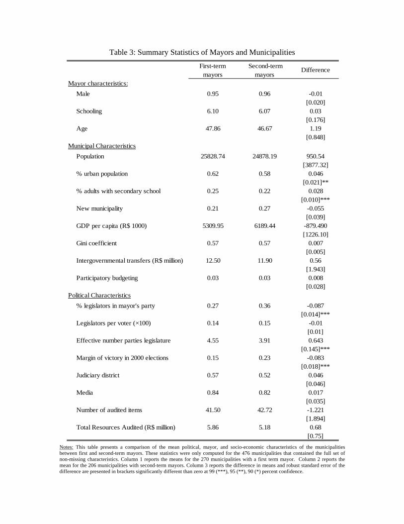
Table 3: Summary Statistics of Mayors and Municipalities

First-term

mayors Second-term

mayorsDifference

Mayor characteristics:Male 0.95 0.96 -0.01

[0.020]Schooling 6.10 6.07 0.03

[0.176]Age 47.86 46.67 1.19

[0.848]Municipal Characteristics

Population 25828.74 24878.19 950.54[3877.32]

% urban population 0.62 0.58 0.046[0.021]**

% adults with secondary school 0.25 0.22 0.028[0.010]***

New municipality 0.21 0.27 -0.055[0.039]

GDP per capita (R$ 1000) 5309.95 6189.44 -879.490[1226.10]

Gini coefficient 0.57 0.57 0.007[0.005]

Intergovernmental transfers (R$ million) 12.50 11.90 0.56[1.943]

Participatory budgeting 0.03 0.03 0.008[0.028]

Political Characteristics% legislators in mayor's party 0.27 0.36 -0.087

[0.014]***Legislators per voter (×100) 0.14 0.15 -0.01

[0.01]Effective number parties legislature 4.55 3.91 0.643

[0.145]***Margin of victory in 2000 elections 0.15 0.23 -0.083

[0.018]***Judiciary district 0.57 0.52 0.046

[0.046]Media 0.84 0.82 0.017

[0.035]Number of audited items 41.50 42.72 -1.221

[1.894]Total Resources Audited (R$ million) 5.86 5.18 0.68

[0.75]Notes: This table presents a comparison of the mean political, mayor, and socio-economic characteristics of the municipalities between first and second-term mayors. These statistics were only computed for the 476 municipalities that contained the full set of non-missing characteristics. Column 1 reports the means for the 270 municipalities with a first term mayor. Column 2 reports the mean for the 206 municipalities with second-term mayors. Column 3 reports the difference in means and robust standard error of the difference are presented in brackets significantly different than zero at 99 (***), 95 (**), 90 (*) percent confidence.

Table 4: The Effects of Re-election Incentives on Corruption

Dependent variable:

OLS OLS OLS OLS OLS OLS Matching Tobit(1) (2) (3) (4) (5) (6) (7) (8)

Mayor in first-term -0.019 -0.020 -0.020 -0.024 -0.026 -0.027 -0.028 -0.042[0.009]** [0.010]** [0.010]** [0.011]** [0.011]** [0.011]** [0.010]** [0.012]**

R-squared 0.01 0.08 0.10 0.12 0.14 0.20 n/a n/aNumber of observations 476 476 476 476 476 476 476 476

Mayor characteristics No Yes Yes Yes Yes Yes Yes YesMunicipal characteristics No No Yes Yes Yes Yes Yes YesPolitical and judicial institutions No No No Yes Yes Yes Yes YesLottery intercepts No No No No Yes Yes Yes YesState intercepts No No No No No Yes Yes Yes

Share of audited resources involving corruption

Notes: This table reports the effects of re-election incentives on share of resources found to involve corruption. Columns 1-6 present the results of an OLS regression of the dependent variables listed in that column on an indicator variable for whether the mayor is in his first term. Column 7 estimates the relationship using Abadie and Imbens (2004) matching estimator and Column 8 use a Tobit specification and reports marginal effects. The log likelihood for the Tobit estimation is 194.20. Mayor characteristics include the age, gender, education and party affiliation of the mayor. Municipal characteristics: population expressed in logarithms, percentage of the population that has at least a secondary education, percentage of the population that lives in the urban sector, new municipality, log GDP per capita per in 2002, Gini coefficient. Political and judicial institutions include: effective number of political parties in the legislature, the number of legislator per voter, the share of the legislature that is of the same party as the mayor, and whether the municipality is judiciary district, and the amount of resources sent to the municipal expressed in logarithms. Robust standard errors are displayed in brackets. Significantly different than zero at 99 (***), 95 (**), 90 (*) percent confidence.

Table 5: The Effects of Re-election Incentives on Alternative Measures of Corruption

Dependent variables:

OLS OLS MatchingNegative Bionomial OLS OLS Matching Tobit

(1) (2) (3) (4) (5) (6) (7) (8)

Mayor in first-term -0.388 -0.471 -0.339 -0.456 -0.008 -0.011 -0.010 -0.009[0.158]** [0.148]*** [0.146]** [0.127]** [0.005] [0.004]** [0.005]* [0.005]*

R-squared 0.01 0.43 n/a n/a 0.01 0.45 n/a n/aNumber of Observations 476 476 476 476 476 476 476 476

Mayor characteristics No Yes Yes Yes No Yes Yes YesMunicipal characteristics No Yes Yes Yes No Yes Yes YesPolitical and judicial institutions No Yes Yes Yes No Yes Yes YesLottery intercepts No Yes Yes Yes No Yes Yes YesState intercepts No Yes Yes Yes No Yes Yes Yes

Share of audited items involving corruptionNumbers of irregularities involving corruption

Notes: This table reports the effects of re-election incentives on number of irregularities associated with corruption and the share of service items involving corruption. Columns 1-2 and columns 5-6 present the results of an OLS regression of the dependent variables listed in that column on an indicator variable for whether the mayor is in his first term. Columns 3 and 7 estimate the relationship using Abadie and Imbens (2004) matching estimator; Column 4 uses a negative binomial specification and Column 8 uses a Tobit specification. In both columns 4 and 8, marginal effects are reported. The pseudo-likelihood for the negative binomial specification is -729.68 and the log likelihood for the Tobit is 459.40. Mayor characteristics include the age, gender, education and party affiliation of the mayor. Municipal characteristics: population expressed in logarithms, percentage of the population that has at least a secondary education, percentage of the population that lives in the urban sector, new municipality, log GDP per capita per in 2002, Gini coefficient. Political and judicial institutions include: effective number of political parties in the legislature, the number of legislator per voter, the share of the legislature that is of the same party as the mayor, and whether the municipality is judiciary district, and the amount of resources sent to the municipal expressed in logarithms. Robust standard errors are displayed in brackets. Significantly different than zero at 99 (***), 95 (**), 90 (*) percent confidence.

Table 6: The Effect of Re-Election Incentives on Corruption Controlling for Unobserved Municipal Characteristics

Dependent variable:

Incumbents who run for reelection

in 2000Linear Quadratic Cubic Linear spline

Quadratic spline

Cubic spline

(1) (2) (3) (4) (5) (6) (7)

Mayor in first-term -0.031 -0.039 -0.040 -0.038 -0.043 -0.047 -0.028[0.014]** [0.019]** [0.019]** [0.022]* [0.019]** [0.024]* [0.029]

Observations 328 328 328 328 328 328 328R-squared 0.27 0.27 0.27 0.27 0.27 0.28 0.28

Mayor characteristics Yes Yes Yes Yes Yes Yes YesMunicipal characteristics Yes Yes Yes Yes Yes Yes YesPolitical and judicial institutions Yes Yes Yes Yes Yes Yes YesLottery intercepts Yes Yes Yes Yes Yes Yes YesState intercepts Yes Yes Yes Yes Yes Yes Yes

Share of audited resources involving corruption

Notes: This table reports the effects of re-election incentives on the share of resources involving corruption. The estimation samples in columns 1-7 include only municipalities where the incumbent ran for re-election. In columns 2-4, the functional form assumption for the running variable is specified at the top of each column. Mayor characteristics include the age, gender, education and party affiliation of the mayor. Municipal characteristics: population expressed in logarithms, percentage of the population that has at least a secondary education, percentage of the population that lives in the urban sector, new municipality, log GDP per capita per in 2002, Gini coefficient. Political and judicial institutions include: effective number of political parties in the legislature, the number of legislator per voter, the share of the legislature that is of the same party as the mayor, and whether the municipality is judiciary district, and the amount of resources sent to the municipal expressed in logarithms. Robust standard errors are displayed in brackets. Significantly different than zero at 99 (***), 95 (**), 90 (*) percent confidence.

Table 7: The Effect of Re-Election Incentives on Corruption Controlling for Ability and Experience

Dependent variable:

Second-term and first-term

later re-elected

Second-term and first-term

later re-electedpredicted

Full sample Full sample

Second-term and first-term that served as

previous mayors

Second-term and first-term that

served as mayor or legislator in past

(1) (2) (3) (4) (5) (6)

Mayor in first-term -0.04 -0.034 -0.027 -0.030 -0.038 -0.027[0.013]*** [0.018]* [0.012]** [0.012]** [0.014]*** [0.017]

Mayor with political experience -0.007[0.011]

Number of years in political office 0.008[0.007]

Number of years in political office ² -0.002[0.001]

R-squared 0.27 0.29 0.21 0.21 0.30 0.29Observations 313 294 476 476 287 311

Mayor characteristics Yes Yes Yes Yes Yes YesMunicipal characteristics Yes Yes Yes Yes Yes YesPolitical and judicial institutions Yes Yes Yes Yes Yes YesLottery intercepts Yes Yes Yes Yes Yes YesState intercepts Yes Yes Yes Yes Yes Yes

Share of audited resources involving corruption

Notes: This table reports the effects of re-election incentives on the share of resources involving corruption. Column 1 compares the corruption levels of second term mayors to those of the subset of first term mayors that were re-elected in the subsequent mayor elections. Column 2 compares the corruption levels of second term mayors to those of the subset of first term mayors who were predicted to be re-elected, based on a propensity score. Column 3-4 is estimated on the full sample. Column 5 includes only municipalities with a second-term mayor and first-term mayors who had a mayor in a previous term. Column 6 includes only municipalities with a second-term mayor and first-term mayors who had been either a mayor or legislator in a previous term. Mayor characteristics include the age, gender, education and party affiliation of the mayor. Municipal characteristics: population expressed in logarithms, percentage of the population that has at least a secondary education, percentage of the population that lives in the urban sector, new municipality, log GDP per capita per in 2002, Gini coefficient. Political and judicial institutions include: effective number of political parties in the legislature, the number of legislator per voter, the share of the legislature that is of the same party as the mayor, and whether the municipality is judiciary district, and the amount of resources sent to the municipal expressed in logarithms. Robust standard errors are displayed in brackets. Significantly different than zero at 99 (***), 95 (**), 90 (*) percent confidence.

Table 8: Re-election Incentives and Other Forms of Bad Governance

Dependent variable: Corruption

Full sampleSecond-term and first-term later re-elected

Second-term and first-term that served as

previous mayors Full sample

(1) (2) (3) (4)

Mayor in first-term 0.054 0.069 0.088 -0.036[0.102] [0.151] [0.180] [0.013]***

Observations 366 243 218 366R-squared 0.44 0.50 0.49 0.28

Mayor characteristics Yes Yes Yes YesMunicipal characteristics Yes Yes Yes YesPolitical and judicial institutions Yes Yes Yes YesLottery intercepts Yes Yes Yes YesState intercepts Yes Yes Yes Yes

Share of audited items involving mismanagement

Notes: This table reports the effects of re-election incentives on the share of audited items found to involve acts of mismanagement. Column 1 uses the full sample. Column 2 compares the mismanagement levels of second term mayors to those of the subset of first term mayors that were re-elected in the subsequent mayor elections. Column 3 includes only municipalities with a second-term mayor and first-term mayors who had a mayor in a previous term. Column 4 reports the effects of re-election incentives on corruption for the sample used in estimating the results presented in column 1. Mayor characteristics include the age, gender, education and party affiliation of the mayor. Municipal characteristics: population expressed in logarithms, percentage of the population that has at least a secondary education, percentage of the population that lives in the urban sector, new municipality, log GDP per capita per in 2002, Gini coefficient. Political and judicial institutions include: effective number of political parties in the legislature, the number of legislator per voter, the share of the legislature that is of the same party as the mayor, and whether the municipality is judiciary district, and the amount of resources sent to the municipal expressed in logarithms. Robust standard errors are displayed in brackets. Significantly different than zero at 99 (***), 95 (**), 90 (*) percent confidence.

Notes: This table reports the effects of re-election incentives on the procurement of matching grants. The specification presented in the odd columns include municipal and mayor characteristics and year intercepts, whereas the specifications in the even columns also include municipality fixed-effects and linear time trends interacted with our mayor and municipal covariates. The sample represents yearly data from 2001-2004 for each municipality in our sample. Robust standard errors clustered at the municipality level are displayed in brackets. Significantly different than zero at 99 (***), 95 (**), 90 (*) percent confidence.

Dependent variable: (1) (2) (3) (4) (5) (6)

Mayor in first term × Election(t) 0.140 0.132 2.053 2.002 0.158 0.143[0.049]*** [0.057]** [0.594]*** [0.688]*** [0.050]*** [0.059]**

Mayor in first term × Election(t-1) 0.105 0.100 1.528 1.494 0.118 0.109[0.047]** [0.054]* [0.572]** [0.655]** [0.048]** [0.055]**

Mayor in first term × Election(t-2) 0.080 0.078 1.342 1.325 0.043 0.038[0.035]** [0.040]* [0.425]*** [0.491]*** [0.036] [0.042]

Mayor in first-term -0.058 -1.107 -0.061[0.034]* [0.423]** [0.034]*

F-test: Election(t-1)=Election(t-2) 0.38 0.23 0.15 0.09 2.91 1.95F-test: Election(t)=Election(t-1) 0.59 0.38 0.95 0.66 0.82 0.44F-test: Election(t)=Election(t-3) 2.15 1.33 2.00 1.36 7.44 4.47Observations 1904 1904 1904 1904 1903 1903Number of municipalities 476 476 476 476 476 476R-squared 0.13 0.45 0.14 0.48 0.12 0.44

Year intercepts Y Y Y Y Y YMunicipal and mayor characteristics Y n/a Y n/a Y n/aMunicipality fixed-effects N Y N Y N YMunicipal and mayor characteristic × time trends N Y N Y N Y

Share of the grant receivedReceived a grant Amount of grants per capita

Table 9: Re-election Incentives and Matching Grants

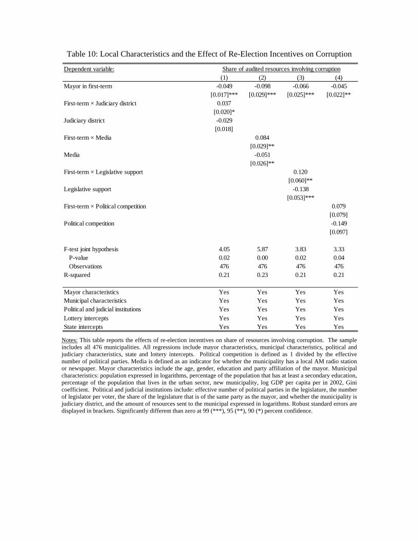
Table 10: Local Characteristics and the Effect of Re-Election Incentives on Corruption

Dependent variable:(1) (2) (3) (4)

Mayor in first-term -0.049 -0.098 -0.066 -0.045[0.017]*** [0.029]*** [0.025]*** [0.022]**

First-term × Judiciary district 0.037[0.020]*

Judiciary district -0.029[0.018]

First-term × Media 0.084[0.029]**

Media -0.051[0.026]**

First-term × Legislative support 0.120[0.060]**

Legislative support -0.138[0.053]***

First-term × Political competition 0.079[0.079]

Political competition -0.149[0.097]

F-test joint hypothesis 4.05 5.87 3.83 3.33P-value 0.02 0.00 0.02 0.04Observations 476 476 476 476

R-squared 0.21 0.23 0.21 0.21

Mayor characteristics Yes Yes Yes YesMunicipal characteristics Yes Yes Yes YesPolitical and judicial institutions Yes Yes Yes YesLottery intercepts Yes Yes Yes YesState intercepts Yes Yes Yes Yes

Share of audited resources involving corruption

Notes: This table reports the effects of re-election incentives on share of resources involving corruption. The sample includes all 476 municipalities. All regressions include mayor characteristics, municipal characteristics, political and judiciary characteristics, state and lottery intercepts. Political competition is defined as 1 divided by the effective number of political parties. Media is defined as an indicator for whether the municipality has a local AM radio station or newspaper. Mayor characteristics include the age, gender, education and party affiliation of the mayor. Municipal characteristics: population expressed in logarithms, percentage of the population that has at least a secondary education, percentage of the population that lives in the urban sector, new municipality, log GDP per capita per in 2002, Gini coefficient. Political and judicial institutions include: effective number of political parties in the legislature, the number of legislator per voter, the share of the legislature that is of the same party as the mayor, and whether the municipality is judiciary district, and the amount of resources sent to the municipal expressed in logarithms. Robust standard errors are displayed in brackets. Significantly different than zero at 99 (***), 95 (**), 90 (*) percent confidence.

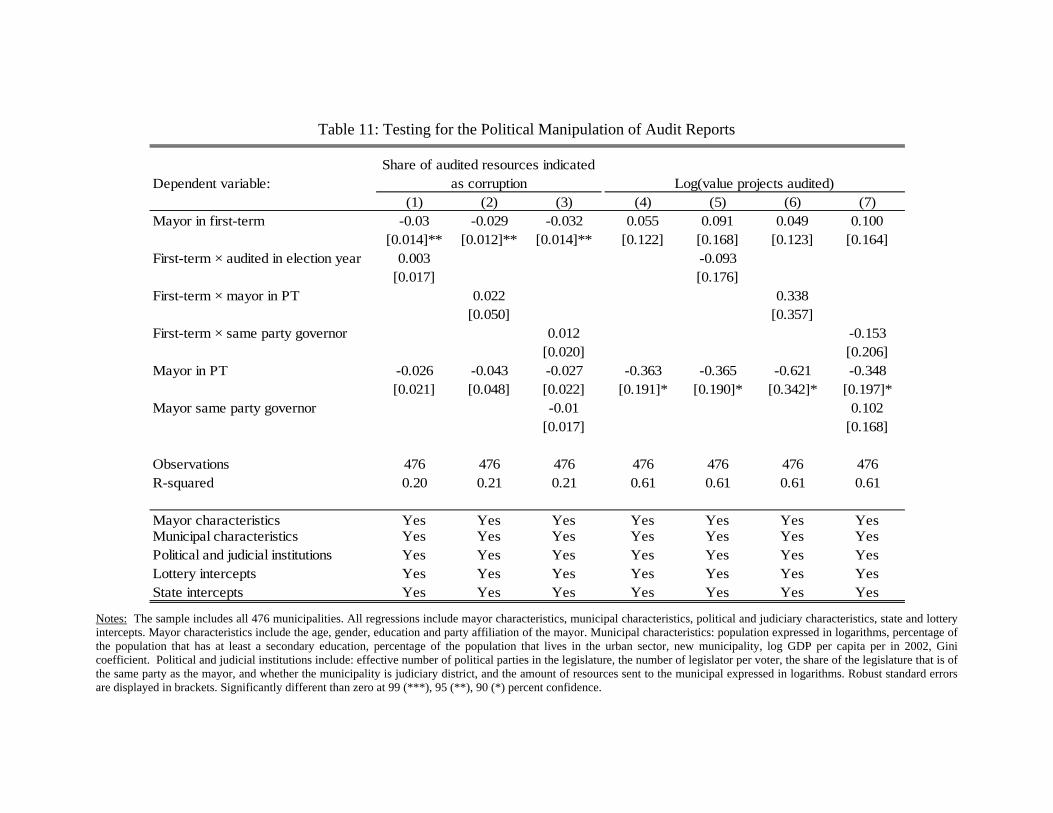
Table 11: Testing for the Political Manipulation of Audit Reports

Dependent variable:(1) (2) (3) (4) (5) (6) (7)

Mayor in first-term -0.03 -0.029 -0.032 0.055 0.091 0.049 0.100[0.014]** [0.012]** [0.014]** [0.122] [0.168] [0.123] [0.164]

First-term × audited in election year 0.003 -0.093[0.017] [0.176]

First-term × mayor in PT 0.022 0.338[0.050] [0.357]

First-term × same party governor 0.012 -0.153[0.020] [0.206]

Mayor in PT -0.026 -0.043 -0.027 -0.363 -0.365 -0.621 -0.348[0.021] [0.048] [0.022] [0.191]* [0.190]* [0.342]* [0.197]*

Mayor same party governor -0.01 0.102[0.017] [0.168]

Observations 476 476 476 476 476 476 476R-squared 0.20 0.21 0.21 0.61 0.61 0.61 0.61

Mayor characteristics Yes Yes Yes Yes Yes Yes YesMunicipal characteristics Yes Yes Yes Yes Yes Yes YesPolitical and judicial institutions Yes Yes Yes Yes Yes Yes YesLottery intercepts Yes Yes Yes Yes Yes Yes YesState intercepts Yes Yes Yes Yes Yes Yes Yes

Share of audited resources indicated as corruption Log(value projects audited)

Notes: The sample includes all 476 municipalities. All regressions include mayor characteristics, municipal characteristics, political and judiciary characteristics, state and lottery intercepts. Mayor characteristics include the age, gender, education and party affiliation of the mayor. Municipal characteristics: population expressed in logarithms, percentage of the population that has at least a secondary education, percentage of the population that lives in the urban sector, new municipality, log GDP per capita per in 2002, Gini coefficient. Political and judicial institutions include: effective number of political parties in the legislature, the number of legislator per voter, the share of the legislature that is of the same party as the mayor, and whether the municipality is judiciary district, and the amount of resources sent to the municipal expressed in logarithms. Robust standard errors are displayed in brackets. Significantly different than zero at 99 (***), 95 (**), 90 (*) percent confidence.

Federal funds that were audited by CGU

Audit program introduced

Constitutional amendment allowing incumbent

mayors to be re-elected

1996 2000 2004Elections→

FIGURE 1: TIMELINE OF THE ELECTORAL CYCLES AND AUDIT TIMING

Notes: Figure shows the timing of Brazil’s municipal elections and the introduction of the audit program. It also depicts the period over which the federal funds were audited and when the constitutional amendment allowing for a second consecutive term in office took place.

FIGURE 2: THE EFFECTS OF RE-ELECTION INCENTIVES ON CORRUPTION

Notes: Figure shows the share of audited resources involving corruption by the margin of victory for incumbents who ran for re-election in 2000. Each figure presents mean corruption for a bin size of 30 percentage points (hollow-circles) along with the fitted values from a 3rd degree polynomial fit on each side of the discontinuity. The dashed lines denote 90 percent confidence intervals. These estimates were computed for a sample size of 328 municipalities.

0.0

5.1

.15

Cor

rupt

ion

-.4 -.2 0 .2 .4 .6Margin of victory