electoral systems and public spending* in modern democracies, elected

ELECTORAL SYSTEMS AND PUBLIC SPENDING*

GIAN MARIA MILESI-FERRETTI

ROBERTO PEROTTI

MASSIMO ROSTAGNO

We study the effects of electoral institutions on the size and composition ofpublic expenditure in OECD and Latin American countries. We emphasize thedistinction between purchases of goods and services, which are easier to targetgeographically, and transfers, which are easier to target across social groups. Wepresent a theoretical model in which voters anticipating government policymak-ing under different electoral systems have an incentive to elect representativesmore prone to transfer (public good) spending in proportional (majoritarian)systems. The model also predicts higher total primary spending in proportional(majoritarian) systems when the share of transfer spending is high (low). Afterdefining rigorous measures of proportionality to be used in the empirical investi-gation, we find considerable support for our predictions.

I. INTRODUCTION

In modern democracies, elected representatives making de-cisions on fiscal policy face a basic trade-off between allegiance toa social constituency and allegiance to a geographic constituency.Elected officials represent a specific district, but also typicallyadvance the interests of specific social groups that spread acrossmany districts or the whole nation. This trade-off is relevant tofiscal policymaking because it parallels the distinction betweenthe two main types of government spending: transfers and pur-chases of goods and services. The former are mostly targeted togroups of individuals with certain social characteristics, such asthe unemployed and the elderly; the scope for targeting themgeographically is therefore limited. The latter (which we will callpublic goods) instead are typically targeted along geographicallines.

* For useful comments and suggestions, we thank Alberto Alesina, V. V.Chari, Torsten Persson, Guido Tabellini, Jose Tavares, two anonymous referees,and participants at seminars at Ente Einaudi in Rome, New York University, YaleUniversity, and the University of California, Los Angeles. We are grateful toArend Lijphart for generously sharing his data. Ernesto Talvi helped us withelectoral results from Uruguay, Jo Buelens provided much needed clarificationson the Belgian electoral system, and Asbjorn Fidjestol on the Norwegian system.Jeffrey Frieden, Mark Hallerberg, Ron Rogowski, Ernesto Stein, and Paul Zackgave us useful bibliographical suggestions. Manzoor Gill and Nada Mora providedexcellent research assistance. The views expressed in this paper do not necessar-ily reflect those of the International Monetary Fund or the European CentralBank. Roberto Perotti is grateful to the National Science Foundation for financialsupport.

© 2002 by the President and Fellows of Harvard College and the Massachusetts Institute ofTechnology.The Quarterly Journal of Economics, May 2002

609

In this paper we study how the electoral system shapes thistrade-off and the incentives of elected officials to allocate reve-nues to the two types of spending. We show that proportionalsystems are more geared to spending on transfers, while majori-tarian systems are more prone to public good spending. Thus,loosely speaking, our model captures the widespread notion that“proportional systems allow representation of a greater variety ofinterests” (a frequent claim by advocates of this system), while“majoritarian systems are more grounded in local interests.”

The model is based on the logic of strategic delegation ofChari, Jones, and Marimon [1997] and Besley and Coate [1999],extended to a framework with two types of government spendingand with different electoral systems. In a majoritarian system,each district elects one representative. If the distribution of dif-ferent social groups is similar across districts, all representativeswill belong to the same social group. Hence, all elected represen-tatives derive utility from the same type of transfers, but eachderives utility from a different public good. It follows that electorswill have an incentive to vote for individuals with stronger pref-erences for public goods relative to transfers, in order to biasgovernment expenditure on public goods toward their district. Inequilibrium the result is just high expenditure on public goods.

In a proportional system, each district elects more than onerepresentative. Hence, more than one social group will be repre-sented in Parliament; in contrast to the majoritarian system,each representative now derives utility from a different type oftransfer. Individuals have an incentive to vote for representativeswith stronger preference for transfers, in order to bias the spend-ing decisions of the government toward their own type of trans-fers. In equilibrium, high spending on transfers is the result. Themodel then predicts that spending on transfers is higher in pro-portional systems, and spending on public goods is higher inmajoritarian systems. Total government spending is higher inproportional systems if the median voter values relatively littlethe public good and relatively highly private consumption andtransfers, lower in the opposite case.

One virtue of our model is that it captures common and, webelieve, plausible views both of the properties of different elec-toral systems and of different types of government spending.Other recent positive models of electoral systems—such as Pers-son and Tabellini [1999a, 2000] and Lizzeri and Persico [2001]—exploit the differences between alternative types of government

610 QUARTERLY JOURNAL OF ECONOMICS

spending, but they emphasize a different breakdown, that be-tween a “universal” expenditure and a more targetable one. Ourmodel does not have a universal type of spending, but two typesof goods with different targeting characteristics: this is whatgenerates the dichotomy between “allegiance to social constitu-encies” and “allegiance to geographic constituencies,” and thatbetween “greater variety of interests” in proportional systems and“greater importance of local interests” in majoritarian systems.1

In the empirical part of this paper, we construct rigorouslydefined measures of the degree of proportionality of electoralsystems in OECD and Latin American countries, and use them toexplore the reduced-form relationship between electoral systemsand government spending. In both cross-section and panel regres-sions, we find considerable support for the predictions of ourmodel for OECD countries, and weaker results for Latin America.In particular, we document the existence of a strong and veryrobust positive relationship between the degree of proportionalityof the electoral system and the size of transfer spending amongOECD countries.

The plan of the paper is as follows. The next section presentsthe model. Sections III and IV solve it in the majoritarian andproportional systems, respectively. Sections V and VI discuss howto operationalize voting systems in view of an empirical test of themodel. Section VII presents the cross-sectional evidence; SectionVIII the panel evidence. Section IX discusses further the relation-ship to the recent literature, both theoretical and empirical. Sec-tion X concludes. Some of the more technical passages in thesolution of the model are presented in Appendix 1; details on theconstruction of the electoral variables are given in Appendix 2;Appendix 3 presents the data.

1. We discuss these models more in detail in Section IX; an importantdifference with our model is that they allow for binding promises by candidates,which we rule out. We also rule out strategic voting. Austen-Smith and Banks[1988] and Baron and Diermeier [2001] show in different contexts how voters canbehave strategically in their electoral decision, internalizing the expected coali-tion bargaining that will lead to policy formation after the election. Strategicvoting can lead electors to pick a party whose preferences or policy platform aremore distant from theirs than another party’s. Key issues are how the right topropose a government coalition is attributed (typically depending on vote shares)and what is each party’s utility out of the status quo outcome in case an agreementis not reached. As we will see, these issues do not arise in our model, because theright to form a government is attributed randomly and all representatives whorefuse an offer to take part in the government receive the same utility.

611ELECTORAL SYSTEMS AND PUBLIC SPENDING

II. THE MODEL

II.1. Population and the Fiscal System

The country is populated by a continuum of individuals, withtotal mass 1. The population is divided into three groups, A, B,and C, with size �A, �B, and �C, respectively. These sizes can bedifferent, but no group can include more than 50 percent or lessthan 25 percent of the population.2 The country is composed ofthree geographic regions. A region can be thought of as the basicsubnational unit of the country: hence, government spendingcannot be targeted more finely than a region.

There are two types of government spending: transfers andpurchases of goods and services, or “public goods.” Typically, thegovernment fixes the eligibility criteria for a specific transfer, andall citizens who meet the criteria are then eligible for that trans-fer, regardless of their region of residence. For instance, old agepensions are paid to all national residents above a certain agewho have paid enough contributions, and unemployment benefitsare paid to all unemployed individuals with a work history. Incontrast, spending on goods and services is local in nature. Thegovernment can always decide to build a school or to hire morepolicemen in a city and not in another; it is a matter of policy howevenly distributed these expenditures are on the national territory.3

Of course, the distinction is not always precise. Certain goodsor services purchased by the government are available virtuallyto the whole population (for instance, a plane in a state-ownedairline company). But it is rarer for transfers to households pro-vided by the central government to be explicitly localized: legis-lation usually does not bar citizens from a certain transfer onlybecause of where they live.4 Thus, we believe that, by and large,the distinction we have made is conceptually and empiricallysound.

We capture this difference between the two types of govern-

2. As we will see, this condition ensures that all three groups are representedin a proportional system.

3. Some public goods—such as defense—clearly have a nationwide external-ity. However, expenditure on these goods is still localized: a military base can bebuilt in a specific state. Ceteris paribus, residents of a state prefer to have themilitary base in their own state than in another state.

4. Of course, transfers can end up being more concentrated in certain areasbecause of the demographic or labor market characteristics of these areas: thus,Florida receives more old-age pension expenditure per person than most otherstates, and high-unemployment areas receive a larger share of unemployment-related transfers.


ment spending in a simple way. Because of some different under-lying characteristics, individuals in the three groups differ in thetypes of transfers they are entitled to: an individual in group jbenefits from the transfer sj, but not from the transfers specific tothe other groups. In contrast, individuals in region k derive utilityfrom public good spending in region k, gk, and not from the publicgoods specific to the other regions.

All individuals have the same productivity, which we nor-malize at 1. The utility of individual i of group j in region k is

(1) Uijk � �1 � t��i�isj�i�1 � �i�gk

1 � �i,

where t is the proportional tax rate, and (1 � t) is therefore anindividual’s posttax income. Thus, individuals have Cobb-Doug-las preferences over public goods and private income, and Cobb-Douglas preferences over the breakdown of disposable incomeinto primary income and transfer income. Within each group, theparameters �i and �i are distributed uniformly over the intervals[�L,�H] and [�L,�H], respectively, with �L, �L � 0 and �H, �H �1.5

II.2. The Electoral System and Government Formation

The values of taxes t, transfers sj, and public goods gk, aredecided by elected representatives. We describe first how repre-sentatives are elected, and then how their preferences are aggre-gated to deliver the policy outcomes [t,sj,gk].

The first stage corresponds to the electoral system. We fix thenumber of representatives at three, and characterize an electoralsystem by the number of electoral districts. At one extreme, eachof the three regions is a separate electoral district electing onerepresentative; we call this the majoritarian system. At theother extreme, the whole country makes up a single electoraldistrict, electing three representatives; we call this the propor-tional system.

Representatives of group j from different regions all deriveutility from the same transfer sj, but from different public goods.When a district comprises more than one region, as in the pro-portional system, it is not necessary for our purposes to specify

5. The assumption of a uniform distribution ensures the existence of a non-cycling majority when individuals vote on the two issues contemporaneously. Theassumption could be relaxed if we assumed that voting on the two issues issequential—see Appendix 1.


fully the process by which public good spending within the dis-trict is then allocated to the regions within the district; we simplyassume that, whatever process is in place, the equilibrium out-come is a uniform allocation of total public good spending amongthe regions.6 Our model focuses on the allocation to districts atthe central government level; in turn, in deciding its allocation,the central government takes into account that it will be dividedequally among the regions in the district.

The second stage describes how governments are formed andhow their decisions are taken. The literature has provided a largenumber of possibilities here. In our setup, one simple way toformalize government formation is the following. One of the threerepresentatives (the Prime Minister) is randomly selected to forma government. He makes an offer to join the government toanother representative, subject to the constraint that the govern-ment maximizes the joint utility of its members. If the secondrepresentative accepts, the government is formed, and policy isdecided by maximizing the joint utility function of the two repre-sentatives. If the second representative does not accept, thePrime Minister makes an offer to the third representative. If healso refuses, then no spending on transfers and public goods isauthorized, and all representatives receive a status-quo utility ofzero. It should be clear that (i) it is not in the interest of the PrimeMinister to offer more than one representative to join the govern-ment; (ii) it is in the interest of a representative to accept an offerby the Prime Minister.7

Besides its simplicity, this formulation of the political processhas the important virtue that it separates the electoral systemfrom the formation of government; that is, electoral systems differonly in the way representatives are elected, and not in the waygovernments are assumed to be formed.

6. The within-district allocation can be interpreted as a subnational voting orbargaining process that takes as given the total amount of public goods allocatedto that district by the central government. All results would go through even if wetreated the subnational governments symmetrically to the national government:namely, the subnational government at the district level is formed by the repre-sentative of a randomly chosen subregion, who then invites the representativefrom another subregion to join the government.

7. The assumption that the government has to maximize the joint utility ofits members reduces the importance of agenda control. As an alternative, we couldassume that two of the three representatives are selected at random to form agovernment. If they agree, the government is formed, and policy is decided bymaximizing a joint utility function. If they do not, then no spending on eithertransfers or public goods can be authorized, and all representatives receive astatus quo utility of 0.


III. MAJORITARIAN SYSTEM

In this system each of the three districts elects one represen-tative. We solve the model backward, starting with the policieschosen by the government.

III.1. The Policy Formation in the Government

In our main analysis we shall assume for simplicity that onegroup is larger than the other two.8 Because all districts have thesame composition, the three representatives will all belong to thelargest group. Assume that group B is such a group: thus, thegovernment will be composed of two B-individuals, elected in twodifferent districts. Denote by k1 and k2 the districts where thetwo members of the government have been elected, and let anasterisk denote an elected individual. Taking logs, the govern-ment will maximize the joint utility:

(2) VM�k1, k2� � ��*k1�*k1 � �*k2�*k2� log �1 � t� � ��*k1�1 � �*k1�

� �*k2�1 � �*k2�� log sB � �1 � �*k1� log gk1 � �1 � �*k2� log gk2,

where the superscript M denotes a majoritarian system and �*ki

and �*kirepresent the preferences of the individuals elected in

district ki. These representatives (and their constituencies) wantdifferent public goods, but both derive utility only from the trans-fer sB. Maximization of the above objective function is subject tothe government budget constraint,

(3) t � �BsB � gk1 � gk2,

where t is the proportional tax rate and the aggregate income ofthe economy is 1. To understand the above expression, recall thatthe per capita transfer is sB: only individuals of type B (a fraction�B of the population) receive it: there is no reason for the tworepresentatives in the government to vote for a positive transferthat benefits the other two groups.

Let s� j � �jsj denote total spending on transfers to group j; lets� , g, and t denote the shares in GDP of transfers, expenditure onthe public goods and total expenditure, i.e., s� � ¥j�A

C �jsj; g �

8. The assumption that a group larger than the others exists considerablysimplifies the algebra in the majoritarian case, but in no way is it essential to ourargument. All our results would go through if we assumed that all groups have thesame size one-third—see the discussion at the end of this section.


¥k�13 gk, and t � s� g. It is straightforward to show that the

government policies that maximize (2) are

(4)

tM�k1,k2� �2 � ��*k1�*k1 � �*k2�*k2�

2

s�BM�k1,k2� �

�*k1�1 � �*k1� � �*k2�1 � �*k2�

2 ; s�AM�k1,k2� � 0; s�C

M�k1,k2� � 0

gk1M�k1,k2� �

1 � �*k1

2 ; gk2M�k1,k2� �

1 � �*k2

2 ; gk3M�k1,k2� � 0

gM�k1,k2� � gk1M�k1,k2� � gk2

M�k1,k2� �2 � �*k1 � �*k2

2 ,

where tM(k1,k2) indicates the equilibrium value of total primaryspending in the majoritarian system when the government isformed by representatives from districts k1 and k2, and similarlyfor the other fiscal policy variables. Similar results obtain in thecase that all groups have the same size.9

III.2. The Choice of the Representatives

In the first stage, each group selects simultaneously by ma-jority voting its own representative among its members, so thatthe space of possible candidates spans the rectangle with length[�L,�H] and height [�L,�H]. In Appendix 1 we show that theindividual with median values of the parameters � and � is thedecisive voter in each group, despite the fact that the issue spaceis bi-dimensional. The median voter of group B in region k1maximizes with respect to �*k1

and �*k1the utility function,10

9. When all groups are the same size, the election result is random. In thiscase we have two possible outcomes for government formation. The first occurs ifthe government is formed by two representatives belonging to the same socialgroup. In this case the policy choice is analogous to the one in equation (4) above.The second outcome occurs if the government coalition is formed between tworepresentatives belonging to different social groups (this will always occur whenthree candidates belonging to different parties are elected). In this case theoptimal policy choice will be analogous to the one of equation (4) for taxation andpublic good spending (with the subscripts k1, k2 now indicating representativesfrom different social groups as well as regions); for transfer spending, the totalis unchanged, but its composition now reflects the preferences of the two so-cial groups in government, with s�k1

M(k1,k2) � ��*k1�1 � �*k1��/ 2 and s�k2M(k1,k2) �

��*k2�1 � �*k2��/2 .10. For simplicity, we omit the social group and region subscripts from the

utility parameters.


(5) E�VmBk1M � � �

r�2

3

�m�m log �1 � tM�k1,kr��

� �m�1 � �m� log sBM�k1,kr� � �1 � �m� log gk1

M�k1,kr��,

where tM (k1,kr), sBM (k1,kr), and gk1

M (k1,kr) are given by (4).Taking first-order conditions and imposing symmetry betweenthe two districts, we obtain the �* and �* preferred by the medianvoter in a majoritarian system:

(6) �*M ��m

2 � �m; �*M � �m.

Hence, the median voter wants a representative with the medianvalue of � but a value of � below the median. The logic is similarto that of Besley and Coate [1999], except that there are two typesof public expenditures. In a majoritarian system, all representa-tives and members of the government benefit from the sametransfer, but from different public goods. Hence, the median voterin district k tries to bias the decision of the government towardhis own public good by electing an individual with preference forhigh spending on public goods relative to transfers. In equilib-rium the result is just high spending on the two public goods thatget funded.

Substituting (6) into (4), one finally gets

tM � 1 ��m�m

2 � �m

(7) s� M ��m�1 � �m�

2 � �m

gM �2�1 � �m�

2 � �m.

Again, similar results obtain when all groups have the samesize.11

11. In this case, the solution for the values of �* and �* chosen by the medianvoter for each party representative in the district turns out to be a weightedaverage of the values in equation (6) and of those that occur under a proportionalsystem (see equation (12) below). The weights are equal to the respective proba-bilities that a government will be formed by two representatives of the same partyor by representatives of two different parties. Results are available from theauthors upon request.


IV. PROPORTIONAL SYSTEM

Because each group has more than 25 percent but less than50 percent of total population, in this system a representativefrom each group is elected.

IV.1. The Policy Formation in the Government

Suppose that the government is formed by representatives ofgroup j1 and j2, who maximize joint utility12

(8) VP� j1, j2� � ��*j1�*j1 � �*j2�*j2� log �1 � t� � �*j1�1 � �*j1� log sj1

� �*j2�1 � �*j2� log sj2 � �2 � �*j1 � �*j2� log �g/3�,

where �*j1and �*j1

are the two utility parameters of the represen-tative from group j1, and similarly for �*j2

and �*j2. The maximi-

zation of the above objective function is subject to the governmentbudget constraint,

(9) t � �j1sj1 � �j2sj2 � g.

It is straightforward to show that the solutions to this problemare

(10)

tP� j1, j2� �2 � ��*j1�*j1 � �*j2�*j2�

2

s� j1P� j1, j2� �

�*j1�1 � �*j1�2 ; s� j2

P� j1, j2� ��*j2�1 � �*j2�

2 ; s� j3P� j1, j2� � 0

s� P� j1, j2� � s� j1P � s� j2

P ��*j1�1 � �*j1� � �*j2�1 � �*j2�

2

gP� j1, j2� � gj1P� j1, j2� � gj2

P� j1, j2� � gj3P� j1, j2� �

2 � �*j1 � �*j22 .

For given �* and �*, total spending on each of the two instru-ments is the same as under a majoritarian system (see equation(4)); however, the optimal choices of �* and �* by the medianvoters will now be different, as we show next.

12. Because in equilibrium public good spending is divided equally within thedistrict, individuals are indifferent to the region of origin of a representative: theonly relevant characteristic is to which social group the representative belongs.


IV.2. The Choice of the Representatives

The median voter of group j1 maximizes with respect to �*j1

and �*j1the utility function:13

(11) E�Vj1mP ��

r�2

3

�m�m log �1�tP� j1, jr��m�1��m� log sj1P� j1, jr�

�1��m� log gP� j1, jr��,

where the values of tP, sj2

P, and gP are given by (10). Takingfirst-order conditions and imposing symmetry between the twogroups, the values of � and � preferred by the median voter in theproportional system are

(12) �*P ��m

2 � �m; �*P �

�m�2 � �m�

1 � �m�1 � �m�.

Hence, the median voter selects a candidate with � higher and �lower than the median. This pattern is exactly the opposite thatunder a majoritarian system. The reason is intuitive: in a propor-tional system, spending on public goods is uniform across regions,but each member of the government benefits from a different typeof transfer. Hence, the median voter tries to bias the decision ofthe government toward his own transfer by electing an individualwith a preference for high spending on transfers relative to publicgoods. In equilibrium the result is just high spending on the twotypes of transfers that get funded. Using (12) in (10), one finallygets

tP �1 � �m�1 � 2�m�

1 � �m�1 � �m�

(13) s� P �2�m�1 � �m�

1 � �m�1 � �m�

gP �1 � �m

1 � �m�1 � �m�.

13. Again, when this does not create any ambiguity, we omit the region andthe group subscripts.


IV.3. Predictions

Comparing equations (6) and (13), it is easy to see that

s� P � s� M

(14) gP � gM

tP � tM7�m �1

�2 � �m�.

Thus, the model delivers three predictions. First, suppose thatone compares the outcome across electoral systems, holding con-stant the median voter’s preference parameters; then we havejust shown that

1. spending on transfers is higher in a proportional system;and

2. spending on goods and services is higher in a majoritariansystem.

Now consider two countries, with different values of �m and�m. In the first, transfers are larger than public good spendingunder both electoral systems: from (7) and (13) this implies that�m � 2/(3 � �m). In the second country, public good spending islarger under both electoral systems, implying that �m 1/(3 �2�m). For �m 1, 2/(3 � �m) � 1/(2 � �m); hence, from (14) inthe first country total spending is larger in a proportional system:tP � tM. Conversely, because 1/(3 � 2�m) 1/(2 � �m), againfrom (14) in the second country, total spending is lower in aproportional system: tM � tP. Hence, we have the third predictionof the model:

3. Total government spending is higher in a proportionalsystem if transfer spending is large relative to public goodspending, regardless of the electoral system; conversely,total government spending is higher in a majoritariansystem if transfer spending is low relative to public goodspending, regardless of the electoral system.

Note that these results also hold when we compare the twoelectoral systems holding constant the number of parties in Par-liament or in government. For example, when all social groupshave the same size, we can have three parties in Parliament evenin a majoritarian system. However, while for given preferences ofthe representatives the collective choices concerning public spend-ing would be the same as in a proportional system, it is still thecase that the representatives chosen under a majoritarian systemhave a stronger preference for public goods’ spending. In fact,


when selecting candidates voters internalize the higher likeli-hood of a conflict of interest in government between public spend-ing priorities than between transfer priorities.

V. OPERATIONALIZING VOTING SYSTEMS

To test these hypotheses, we need quantitative measures ofthe degree of proportionality of a system. The key variable weconstruct is the share of electoral votes that guarantees a party aparliamentary seat in an electoral district of average size. Thisvariable, formally defined in subsection V.2, is denoted by UMS(upper marginal share). Clearly, the more proportional is a sys-tem, the easier it is for small parties to gain political representa-tion, and hence proportionality is declining in the UMS.

Constructing such measure is not a straightforward matter,however, because real-life electoral systems are invariably morecomplicated than the stylized systems of the model. Three fea-tures of actual electoral systems need to be taken into accountwhen constructing measures of proportionality: the number oftiers used to allocate seats; the presence or absence of legalthresholds to bar smaller parties from entering parliament; andthe method used for translating seats into votes.

V.1. Electoral Tiers

Electoral systems in general have one or two tiers. In two-tiersystems, a certain portion of parliamentary seats are allocated ina second tier comprising fewer, larger districts, each encompass-ing several first-tier districts. This second tier typically serves thefunction of increasing the degree of proportionality in the elec-toral system. We will use T1 and T2 as shortcuts for “first tier”and “second tier.”

Let Sik denotes the number of seats attributed to parties onthe basis of votes in district k of tier i,14 or its district size; Si �¥k Sik is the total number of seats attributed to parties on thebasis of votes in tier i, or the tier size; Di is the number ofdistricts in tier i; S� i � Si/Di is the average district size of tier i.15

14. The subscripts i and k in this section have a different meaning from thesame letters in the presentation of the model (Sections II–IV).

15. In some electoral systems (see subsection V.4), S1k can be an upper boundto the number of seats attributed in a T1 district: some seats could be left unfilled,transferred to T2, and attributed there; in these cases, the number of seatsattributed in T2 depends on the number of seats effectively attributed in T1.


As is standard in the literature, whenever there are two cham-bers, all of these magnitudes refer to the lower chamber.

V.2. Voting Method

A voting method describes how party votes are converted intoseats in each district of an electoral system. We distinguish be-tween three voting methods:

1. Majority/Plurality. All the Sik district seats are attributedto those parties that win an absolute majority of votes(Majority systems) or just more votes than other candi-dates/lists (Plurality systems). In our sample, Majoritymethods are represented by the Two-Round method(France) and the Alternative Vote method (Australia);16

Plurality methods are represented by the First-Past-the-Post method (United Kingdom and several others).

2. Highest Average. The share of votes obtained by eachparty in each district is divided sequentially by a set ofdivisors: 1, 2, 3, . . . in the case of the d’Hondt formula, and1,3,5, . . . in the case of the St. Lague formula. Each of theSik highest quotients entitles the party that obtains themto a seat.17

3. Largest Remainder. In each district k of tier i, first a quotais calculated, defined as 1/Sik in the Hare formula,1/(Sik 1) in the Droop formula, and 1/(Sik 2) in theImperiali formula. Then each party is allocated as manyseats as full quotas it has obtained. The seats left unfilledafter this allocation can be transferred to a higher tier, ifit exists, or attributed in the same district to the parties orcandidates with the largest remainders.18

16. In the Australian system, voters rank candidates on the ballot. Any candi-date with an absolute majority is elected. If no candidate reaches an absolute major-ity, the candidate with the lowest number of first preferences is eliminated, and hisvotes reassigned to all other candidates according to the ranking indicated on hisballots. The process is repeated until a candidate reaches an absolute majority.

17. As an example, consider a four-seat district with three parties (A, B, andC), 100 electors, and votes obtained by each party VA � 50, VB � 30, VC � 20.Under a d’Hondt formula, the quotients obtained by A are 50, 50/2, and 50/3; byB, 30, 30/2, and 30/3; by C, 20, 20/2, and 20/3. The three highest quotients are 50,30, and 50/2. Hence, A gets two seats, B one seat, and C gets no seats.

18. Two methods, the Single Transferable Vote (used in Ireland) and theSingle Nontransferable Vote (used in Japan until 1995) are difficult to fit in ourclassification. In one important respect (the calculation of upper quotas—seebelow) they behave like Largest Remainder methods; hence, we will classify themas such. In the Irish STV method, voters rank candidates. Any candidate whosefirst preferences reach a full Droop quota is elected, and his votes above the quotaare redistributed to the remaining candidates following the second preferences he


V.3. Legal Thresholds

Legal thresholds serve the purpose of limiting access to Par-liament to parties receiving “small” shares of votes. Formally, thelegal threshold of tier i, THRi, is the minimum share of nationalvotes, set by the electoral law, that a party must obtain in orderto be eligible for a seat in the tier.19

V.4. Defining Proportionality of Electoral Systems

We now proceed to construct our measure of proportionality,in three stages. We first determine the share of votes that guar-antees a seat in the average district of each tier, abstracting fromelectoral thresholds. We then take electoral thresholds into ac-count. Finally, we determine in which tier the “marginal seat” isallocated.20

We start by defining the share of votes that, even under themost unfavorable distribution of votes among parties in the dis-trict, still guarantees a seat to the party that obtains it.

DEFINITION (UPPER QUOTA, QI). The upper quota of district k in tieri, Qi(Sik), is the share of district votes that would guaranteea party its first seat in that district, if there were no legalthreshold.

Note that in general the upper quota depends only on thedistrict size, not on the number of parties in the district.21 We

has received. If no candidates reach a full quota, the candidate with the lowestnumber of first preferences is eliminated. The process continues until all Sik seatsare filled. In the Japanese SNTV method, voters express a single vote; theSik most voted candidates are elected.

19. Thus, THR2 � .05 would state that, in order to obtain at least one seatin T2, a party must win at least 5 percent of the national votes. If the samethreshold also applies to T1, a party not meeting this threshold must relinquishany T1 seat that it might have obtained. Otherwise, the threshold is binding onlyfor the allocation of T2 seats. Note that, if a legal threshold does not exist in tieri, this is equivalent to assuming that THRi � 0. Sometimes the electoral lawsstate requirements on the vote shares of a party in a district, rather than a tier.These local requirements can be translated into a share of national votes, andtherefore into a legal threshold, using the procedure described in Appendix 2.

20. To implement our measures of proportionality, we assume that the dis-tribution of votes among parties is the same in all T1 districts. In other words, bythis assumption a party’s district share of votes in all T1 districts is equal to itsnational share. An obvious shortcoming of this assumption is that it does not dealwell with regional parties. However, incorporating regional parties would requirea detailed knowledge of actual results, election by election and district by district,which we do not have.

21. In a few cases (Hare and St. Lague when the number of parties is belowthe district magnitude) the formula for the upper quota depends on the number of


provide formulas for the upper quota for each voting methodin the Appendix.

By taking into account the electoral threshold, we cannow define the share of votes that ensures a party electoralrepresentation in a district of average size in tier i.

DEFINITION (UPPER MARGINAL SHARE OF VOTES OF TIER I, UMSI). Theupper marginal share of votes of tier i, UMSi, is the share ofnational votes that guarantees a seat to a party in the districtof average size of that tier: UMSi � max(Qi(S� i),THRi).

For multitier systems, we also need to establish in whichtier the “marginal” seat is allocated: that tier is the decisivetier for the purpose of determining the degree ofproportionality.

DEFINITION (DECISIVE TIER). The decisive tier of an electoral systemis the tier with the lower Upper Marginal Share of votes.

In other words, the decisive tier is the tier where it iseasier for a small party to gain representation. We can nowdefine our proportionality variable.

DEFINITION (UPPER MARGINAL SHARE OF VOTES OF AN ELECTORAL SYS-TEM, UMS). The upper marginal share of votes of an electoralsystem, UMS, is the share of national votes that guaranteesa seat in the district of average size of the decisive tier: UMS� min(UMS1,UMS2).

V.5. Implementing the Definition

We now show how this definition can be applied in practice tothe different types of electoral systems. The case of one-tier elec-toral systems is straightforward: UMS is just the larger betweenthe upper quota in the average-size district and the electoralthreshold in the only tier; that is, UMS � max(Q1(S� 1),THR1).

Constructing UMS in two-tier systems is more complicated.In order to determine the share of national votes that ensures aseat in the system as a whole, we need to address two issues: first,how is the total number of second-tier seats (S2) determined, andsecond, which votes are used to allocate such seats. Table Isummarizes the two-tier systems in our sample.

parties. In these cases, we have collected data on the number of parties in eachelection.


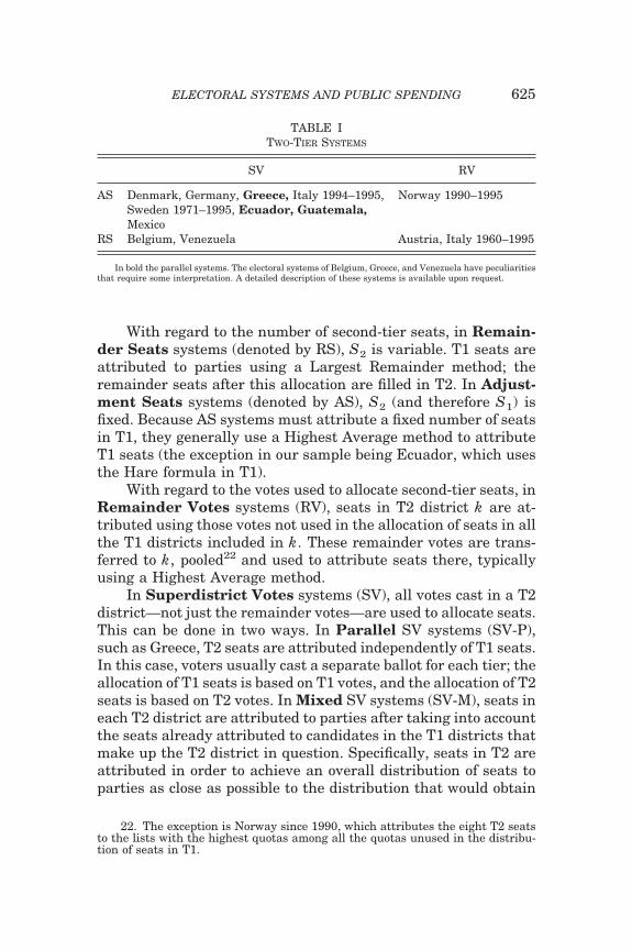
With regard to the number of second-tier seats, in Remain-der Seats systems (denoted by RS), S2 is variable. T1 seats areattributed to parties using a Largest Remainder method; theremainder seats after this allocation are filled in T2. In Adjust-ment Seats systems (denoted by AS), S2 (and therefore S1) isfixed. Because AS systems must attribute a fixed number of seatsin T1, they generally use a Highest Average method to attributeT1 seats (the exception in our sample being Ecuador, which usesthe Hare formula in T1).

With regard to the votes used to allocate second-tier seats, inRemainder Votes systems (RV), seats in T2 district k are at-tributed using those votes not used in the allocation of seats in allthe T1 districts included in k. These remainder votes are trans-ferred to k, pooled22 and used to attribute seats there, typicallyusing a Highest Average method.

In Superdistrict Votes systems (SV), all votes cast in a T2district—not just the remainder votes—are used to allocate seats.This can be done in two ways. In Parallel SV systems (SV-P),such as Greece, T2 seats are attributed independently of T1 seats.In this case, voters usually cast a separate ballot for each tier; theallocation of T1 seats is based on T1 votes, and the allocation of T2seats is based on T2 votes. In Mixed SV systems (SV-M), seats ineach T2 district are attributed to parties after taking into accountthe seats already attributed to candidates in the T1 districts thatmake up the T2 district in question. Specifically, seats in T2 areattributed in order to achieve an overall distribution of seats toparties as close as possible to the distribution that would obtain

22. The exception is Norway since 1990, which attributes the eight T2 seatsto the lists with the highest quotas among all the quotas unused in the distribu-tion of seats in T1.

TABLE ITWO-TIER SYSTEMS

SV RV

AS Denmark, Germany, Greece, Italy 1994–1995,Sweden 1971–1995, Ecuador, Guatemala,Mexico

Norway 1990–1995

RS Belgium, Venezuela Austria, Italy 1960–1995

In bold the parallel systems. The electoral systems of Belgium, Greece, and Venezuela have peculiaritiesthat require some interpretation. A detailed description of these systems is available upon request.


if all seats were attributed based on the T2 votes, method, andnumber of districts. Effectively, then, if there are enough seats inT2, the seats attributed to candidates in T1 serve only to deter-mine the names of as many representatives, but the distributionof seats to parties is determined wholly in T2. Since we areinterested in the distribution of seats to parties, for our purposesthe system effectively works as if S2 � Stot: this is what we willuse in our empirical application.23

We can now turn to the determination of the degree of pro-portionality of two-tier systems. In SV systems we can deter-mine UMS2 by simply applying its definition: UMS2 �max(Q2(S� 2),THR2).24 The purpose of the second tier is to in-crease the proportionality of the system; hence, in all these sys-tems UMS2 UMS1, and T2 is the decisive tier: UMS � UMS2.

In two-tier RV systems the lowest share of national votesthat still guarantees a seat to a party in the average district of T2occurs when the party does not win any T1 seat, transfers all itsvotes as remainders to T2, and these votes are enough to guar-antee a seat in the average district there. Thus, as in SV systemsUMS � UMS2. However, now it is no longer true that the T2shares of votes are the same as the national shares of votes: onlythe remainder votes from T1 are used to allocate T2 seats, andsmall parties (for instance, all those that did not obtain any seatin T1) have a much larger share of remainder votes than of allnational votes. Appendix 2 shows how UMS2 can be calculated inthese cases.

VI. MEASURES OF PROPORTIONALITY

Typically, in the literature (e.g., Taagepera and Shugart[1989] and Lijphart [1994]) proportionality is captured by a mea-sure of district size, rather than by a measure of vote share likeUMS.25 Thus, in this section we first convert UMS into a mea-sure of average district size; then we present two more measures

23. Obviously for the first tier in these systems to be completely irrelevant, asufficient number of seats must be attributed in the second tier. In practice, thisis the case for all SV-M systems in our sample.

24. Although the formula is the same, recall that S2 � Stot in AS/SV-Msystems, while in AS/SV-P systems S2 Stot.

25. Taagepera and Shugart [1989] calculated average effective district mag-nitudes for a number of OECD countries in the seventies and mideighties. Ourmeasure differs from theirs because it is based on the rigorously defined notion ofUpper Marginal Share of votes, which incorporates the different types of two-tiersystems and legal thresholds.


of proportionality, some variants of which have often been used inthe literature. These measures try to formalize how easy it is forsmaller parties to gain representation in Parliament.26

VI.1. Average Standardized District Magnitude (SM)

As made clear in the previous section, UMS is, ceteris pari-bus, inversely related to the average district size of the decisivetier. For instance, in a single-tier electoral system with no thresh-olds, which uses the d’Hondt voting method, UMS is equal to theupper quota in the “average” district: UMS � Q1(S� 1) � 1/(1 S� 1). One can invert the above relation and back out a measure ofaverage district magnitude from data on UMS. In doing so,however, it is important to partial out the voting method used ineach system.27 We use the d’Hondt formula, which does notdepend on the number of parties and therefore provides a one-to-one mapping with UMS. By applying the inverse of the d’Hondtformula to UMS, we thus obtain the Average Standardized Dis-trict Magnitude, or SM. More formally,

DEFINITION (AVERAGE STANDARDIZED DISTRICT MAGNITUDE, SM). Con-sider the electoral system �, possibly with two tiers and alegal threshold; and consider the electoral system �, with onetier, no legal threshold, and the d’Hondt formula. The aver-age standardized district magnitude of system �, SM, is theaverage district size of system � in which a party with thesame UMS of � would be guaranteed a seat.

Hence, SM � S� � � 1/UMS � 1.

26. In constructing these measures of proportionality, we ignore those tierselecting less than 5 percent of the total assembly size. In our sample, this excludesthe second tier in the Norwegian AS/RV system in 1991–1995, which elects 8 outof 165 representatives, and the fourth parallel tier in the Greek AS/SV system,which elects 12 out of 300 representatives.

27. Suppose that two one-tier systems have the same value of UMS of 0.1,but the first uses the St. Lague formula with six parties, the second the d’Hondtformula. Inverting the formulas for the upper quotas in Appendix 2, subsection 2,the average district magnitude would be 8.5 in the first system and 9 in the secondsystem. Hence, it is important to convert the UMS of the system in the averagedistrict size of a standard system, with a fixed electoral formula. In the workingpaper version of this paper [Milesi-Ferretti, Perotti, and Rostagno 2001], we alsoconsider an alternative measure of proportionality which uses the voting methodof the decisive tier of the electoral system to invert the formula for the upperquota. In practice, this measure is very strongly correlated with SM.


VI.2. Average District Magnitude (AM)

A second measure of average effective district magnitudecaptures the notion of how large is the district where the “aver-age” representative is formally elected. It is defined as follows:

DEFINITION (AVERAGE DISTRICT MAGNITUDE, AM). The average dis-trict magnitude of an electoral system is the weighted aver-age of the average district sizes of the two tiers, with weightsequal to the proportion of all representatives elected in thetwo tiers.

Thus, this variable is measured simply by AM � (S1/Stot)S� 1 (S2/Stot)S� 2. Note that, for the purposes of computingthis variable, S1 and S2 represent the number of representativeseffectively elected in each tier.

VI.3. The Average Deviation from Proportionality (RAE)

The two variables described so far are ex ante measures ofproportionality, being based on institutional characteristics. Wealso use one ex post measure, based on voting outcomes electionby election. This variable was originally defined by Rae [1967] asfollows:

DEFINITION (AVERAGE DEVIATION FROM PROPORTIONALITY, RAE). TheAverage Deviation from Proportionality (RAE) is the averageof the deviations (in absolute values) of the share of seats ofeach party from its share of votes: RAE � ¥p � 1

P �sp � vp�,where p indexes a party, sp is the share of seats and vp is theshare of votes obtained by party p.

Thus, this variable measures deviations of the shares of seatsin Parliament from the share of votes obtained by parties in eachelection.28

VII. CROSS-SECTIONAL REGRESSIONS

VII.1. The Data

Our sample consists of twenty OECD and twenty LatinAmerican countries, listed in Appendix 3. The data consist of the

28. This variable is not independent of the number of parties and their size:it tends to give a small degree of disproportionality in systems with many smallparties. An alternative measure, proposed by Gallagher [1991], is defined as thesquare root of the sum of squares of the deviations between seat and votepercentages. Thus, it gives more weight to large deviations. In practice, it is highlycorrelated with RAE.


political variables described in the previous section, the level andcomposition of public spending as well as a number of othercontrol variables described in Appendix 3. The fiscal data includetotal primary government spending, government transfers tohouseholds, and expenditure on public goods, all by the generalgovernment. Transfers are defined as the sum of social securitypayments and other transfers to families, plus subsidies tofirms.29 Public goods are defined as the sum of current and capitalspending on goods and services, i.e., the sum of governmentconsumption and of capital spending.30 The so-called “pork-bar-rel” expenditure, like building a bridge or hiring civil servants ina certain locality to please one own’s constituency, falls mostlyunder one of the two components of our definition of public goods,government consumption and investment.

Data for the OECD sample start in 1960, with the exceptionof Greece, Portugal, and Spain whose data start in the mid-seventies. The time span for Latin American data is more limited—we have information on electoral variables for the early nineties.In our empirical investigation we first use the combined OECDand Latin American samples for cross-sectional estimates (basedon averages of all variables over the four-year period 1991–1994or the closest available periods31), and then we exploit the time-series dimension of the OECD sample to run panel regressions.

Table II displays the cross-sectional 1991–1994 average,standard deviation, minima and maxima for each variable, for thewhole sample as well as for OECD and the Latin Americancountries separately. To make the reading of the empirical resultseasier, we will define all electoral variables as direct measures ofproportionality. To do so, in the case of RAE we take the negativeof the variable as originally defined, although we keep the origi-nal name.

A few points are worth noticing, because they will play a rolein interpreting our results. Latin American countries have, onaverage, more proportional systems. They also have much

29. For most Latin American countries we do not have enough information toseparate social transfers to families from subsidies to firms.

30. The residual term in total primary expenditure is property income paid(net of interest payments), which is also largely not subject to political control ateach moment in time. In the OECD sample, the residual term also includessubsidies to firms.

31. For some Latin American countries, we use a different period wheneverthe electoral law changes during the 1991–1994 period, in order to encompass onlyone electoral law. The details of the time periods used for Latin American coun-tries are in Appendix 3, subsection 1.


TA

BL

EII

SU

MM

AR

YS

TA

TIS

TIC

S

All

Mea

nA

llS

DA

llM

inA

llM

axO

EC

DM

ean

OE

CD

SD

OE

CD

Min

OE

CD

Max

LA

Mea

nL

AS

DL

AM

inL

AM

ax

Avg

.di

stri

ctm

agn

.(A

M)

16.1

30.7

115

015

32.3

115

017

.329

.91

120

Sta

nd.

dist

rict

mag

n.

(SM

)23

.639

.71

180.

820

.133

114

8.3

27.2

461

180.

8R

AE

34.

40.

326

.12.

41.

90.

36.

83.

76.

50.

326

.1P

rim

ary

expe

nd.

/GD

P32

.615

.110

.366

.645

.49.

432

.766

.619

.85.

510

.329

.8T

ran

fers

/GD

P13

.49.

51.

431

.621

.36.

311

.531

.65.

53.

61.

414

.6P

ubl

icgo

ods/

GD

P18

.15.

67.

129

.921

.94.

216

29.9

14.4

4.1

7.1

23.5

GD

Ppe

rca

pita

8400

5500

1200

1810

013

200

2800

6800

1810

035

0018

0012

0072

00P

opu

l.sh

are

over

659.

75.

22.

919

.514

.42

11.3

19.5

52.

22.

911

.8E

ff.

nu

mb.

ofpa

rtie

s3.

51.

71.

38.

43.

71.

61.

98.

43.

31.

71.

38.

4E

TH

NIC

(fra

ct.

inde

x)20

.119

.81

7522

.122

.11

7518

.117

.51.

159

.9O

PE

N(o

pen

nes

s)30

.517

.37.

496

.130

.114

.18.

762

.930

.920

.47.

496

.1

Cro

ss-s

ecti

onal

aver

ages

,sta

nda

rdde

viat

ion

s,m

inim

um

and

max

imu

mva

lues

for

all

the

vari

able

sfo

rth

efu

llsa

mpl

e,th

eO

EC

Dsa

mpl

ean

dth

eL

atin

Am

eric

ansa

mpl

e.S

eeth

eA

ppen

dix

for

vari

able

s’m

nem

onic

s.E

ach

cros

s-se

ctio

nal

obse

rvat

ion

isth

e19

91–1

994

(or

clos

est

avai

labl

epe

riod

)ave

rage

ofth

eva

riab

lefo

rth

eco

un

try.

Nu

mbe

rof

obse

rvat

ion

s:40

for

the

wh

ole

sam

ple

(35

for

RA

E);

20fo

rth

eO

EC

Dsa

mpl

e,20

for

the

Lat

inA

mer

ican

sam

ple

(15

for

RA

E).


smaller governments: average primary expenditure is 19.8 per-cent of GDP, less than half than in OECD countries; indeed, thelargest Latin American government is smaller than the smallestOECD government. The largest difference between the twogroups of countries is in transfers: on average, their ratio to GDPis four times higher in OECD countries; in contrast, the shares ofpublic goods are much closer: 21.9 percent versus 13.9 percent. InLatin America public good spending is much larger than trans-fers, but the two items are virtually equal in OECD countries.32

Table III displays the average values over 1991–1994, coun-try by country, of the electoral variables used in our estimation.Table IV displays the cross-country correlations among the aver-ages of LogAM (the log of Average District Magnitude), LogSM(the log of Average Standardized District Magnitude), MAJ (a

32. Indeed, if one subtracts military spending from public good spending,transfer spending becomes larger than public good spending. The size of militaryspending is to a large extent dictated by international commitments, and itsgeographic targeting may be constrained by strategic considerations.

TABLE IIIAVERAGE VALUES OF ELECTORAL VARIABLES*

AM SM RAE ENPP AM SM RAE ENPP

Australia 1.0 1.0 �5.1 2.4 Argentina 10.7 10.7 3.0Austria 19.4 38.0 �1.0 3.0 Bolivia 14.4 14.9 �2.2 3.3Belgium 8.4 23.6 �1.1 8.4 Brazil 17.8 17.8 �1.8 8.4Canada 1 1 �6.8 2.3 Chile 2.0 2.0 �1.8 5.0Switzerland 7.8 7.8 �0.9 6.3 Colombia 4.9 4.9 3.1Germany 10.8 19.0 �2.0 3.2 Costa Rica 8.1 8.8 �1.8 2.2Denmark 15.3 49.0 �1.0 4.4 Dominican Rep. 30.0 39.0 �2.7 2.9Spain 6.7 6.7 �1.8 2.9 Ecuador 4.4 12.2 6.4Finland 13.3 13.3 �1.4 5.2 El Salvador 4.3 4.3 �2.0 3.0France 1 1 �5.2 3.0 Guatemala 10.1 29.0 �3.4 4.7United Kingdom 1 1 �5.0 2.2 Honduras 6.7 7.9 �1.5 2.0Greece 5.7 10.4 �1.9 2.3 Jamaica 1 1 �26.1 1.3Ireland 4.0 4.0 �1.5 3.2 Mexico 80.6 65.7 �1.2 2.3Italy 17.2 29.3 �1.2 5.5 Nicaragua 10.0 12.3 �0.9 2.1Japan 3.9 3.9 �1.7 3.4 Panama 1.7 1.7 1.4Netherlands 150.0 148.3 �0.3 4.2 Paraguay 4.4 4.4 �1.1 2.5Norway 8.7 8.6 �1.2 4.2 Peru 120 120 3.9Portugal 10.5 10.5 �3.7 2.3 Trin. and Tob. 1 1 �8.1 2.1Sweden 14.1 24.0 �1.0 4.1 Uruguay 5.2 5.2 �0.3 3.3United States 1.0 1.0 �4.7 1.9 Venezuela 7.9 180.8 �0.9 3.4

* AM: Average district magnitude. SM: Average standardized district magnitude. RAE: (minus) index ofdeviations from proportionality. ENPP: effective number of political parties in Parliament. See Section VI andAppendix 3 for further details on the definition of variables.


dummy variable taking the value of one in majoritarian systemsand zero otherwise, from Persson and Tabellini [1999a]); andLogMAGN (the log of the measure of effective district magnitudeby Taagepera and Shugart [1989] and Lijphart [1994], which weextended to 1995 using the same methodology). The high corre-lations between LogSM, LogAM, and LogMAGN, and betweenRAE and MAJ are noteworthy. Table A1, available from theauthors at http://www.iue.it/Personal/Perotti, presents the de-tails, country by country, of each electoral system.

VII.2. Basic Specification

Our basic cross-section specification is

(15) Gi � c � cOECD � �Xi � �POP65i � �LogGDPPCi � �i,

TABLE IVPROPORTIONALITY MEASURES: CROSS-COUNTRY CORRELATIONS (1991–1994)

Log SM Log AM RAE MAJ Log MAGN

Panel A. Whole sample

Log SM 1Log AM 0.92 1RAE 0.52 0.55 1MAJ �0.18 �0.17 �0.58 1

Panel B. OECD

Log SM 1Log AM 0.97 1RAE 0.85 0.84 1MAJ �0.82 �0.82 �0.92 1Log MAGN 0.95 0.95 0.87 �0.87 1

Panel C. Latin America

Log SM 1Log AM 0.86 1RAE 0.52 0.55 1MAJ �0.18 �0.17 �0.58 1

Measures of proportionality calculated as average during the period 1991–1994. AM: Average districtmagnitude. SM: Average standardized district magnitude. RAE: (minus) index of deviations from propor-tionality. MAJ: dummy variable taking the value of one if the electoral system is majoritarian and zerootherwise. MAGN: effective district magnitude. See Section VI and Appendix 3 for more details on thedefinition of variables. The variables SM and AM are available for all countries in the sample. The variableMAGN is available for OECD countries only. The variables RAE and MAJ are available for all OECDcountries and fifteen and eighteen Latin American countries, respectively.


where i indexes a country. G is the average percent share in GDPof either total primary expenditure EXP, transfers TRAN, orpublic goods PGOOD. X is one of the three electoral systemvariables that we have introduced before; the first two, LogAMand LogSM, are the logs of the Average District Magnitude and ofthe Average Standardized District Magnitude, respectively.33

The third electoral variable is RAE. POP65, the share of popula-tion over 65, is a potentially important determinant of the size oftransfer expenditure;34 and LogGDPPC, the PPP adjusted percapita income of the country, in logs of thousands of dollars,captures possible Wagner Law-type effects. In addition to theregression constant, c, we also include an OECD dummy vari-able, cOECD, to allow for the large difference in the averagegovernment spending/GDP ratio between OECD and Latin Ameri-can countries.

Our hypotheses imply that an increase in the value of any ofthe electoral variables should be associated with a higher share oftransfers in GDP—a positive value of � when G � TRAN—andwith a lower share of public goods in GDP—a negative value of �when G � PGOOD (see Results 1 and 2 in subsection IV.3). Inaddition, the effect on total spending depends on the initial shareof transfers in total primary spending, and more fundamentallyon the underlying preferences of the median voter. We havedocumented above the vastly different shares of transfers in GDPand in government spending between Latin American and OECDcountries. If we interpret these differences as reflecting, at leastin part, different patterns of distribution of preferences over fiscalpolicy between these two groups of countries, then when Gi �EXP, we should expect a positive value of � in OECD countries,which have a large share of transfers in primary spending, and anegative value of � in Latin American countries, all of which havean extremely low share of transfers (see Result 3 in subsectionIV.3).

33. We use logs because increasing the average district magnitude by onerepresentative has a very different effect on government spending when the initialdistrict magnitude is 1 than when it is 50.

34. One could argue that POP65 is an endogenous variable, as higher spend-ing on certain types of expenditure (notably health) can increase life expectancy.We cannot think of a good instrument in our sample, but we note that thecorrelation of POP65 with the electoral variable is quite low; in fact, when wereestimate our regressions dropping POP65, the estimated coefficients of theelectoral variables are largely unchanged, and if anything, larger.


VII.3. Basic Results

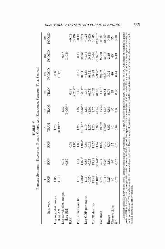
In columns (1)–(3) of Table V the dependent variable is thetotal primary spending/GDP ratio, EXP. The estimated coeffi-cients of the three electoral variables are positive, but none issignificant at conventional levels. This result is consistent withour theoretical model, where a more proportional system canhave an ambiguous impact on total primary government spend-ing, depending on the relative strength of its effects on transferand public good spending. In fact, we will see shortly that thisresult is the combination of two very different patterns in LatinAmerica and in OECD countries.

Our model predicts that more proportional systems should beassociated with higher spending on transfers. Columns (4)–(6)display the same regressions as columns (1)–(3), but with theshare of transfers in GDP as the dependent variable. Now all theestimated coefficients of the electoral variables are significant atthe 5 percent level. To assess the economic significance, considerthe change in the dependent variable associated with a change inthe electoral variable equal to its range (reported in the third tolast row of the table). The range in the transfer/GDP ratio variesbetween about 6.9 (in the LogSM regressions of column (5)) and9.8 percentage points of GDP (in the RAE regression of column(6)). Besides electoral variables, the only other significant vari-able in the regressions is POP65, which has the expected positivecoefficient. Still, the explanatory power of these regressions isquite large, with adjusted R2s always at or above .8.

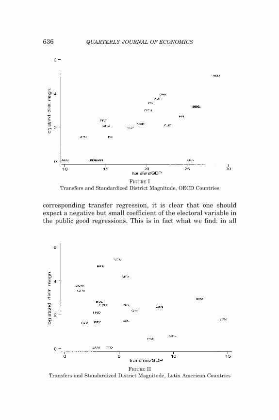
The reader may question whether we are simply capturing adichotomy between majoritarian and proportional systems,rather than a systematic relation between the degree of propor-tionality and transfers. Figure I provides a clear negative answerto this question. It shows that, for OECD countries, the positiverelationship between LogSM and transfers survives (and actuallybecomes stronger) even if one excludes the countries with a ma-jority/plurality system in the sample: Australia, France, UnitedKingdom, Canada, and the United States. A plot of the residualsof a regression of transfers on log GDP per capita and share ofpopulation above 65 (not included for reasons of space) conveysthe same message. In Latin America, by contrast, there is no bivari-ate relation between proportionality and transfers (Figure II).

By comparing the coefficients of the electoral variables ineach total spending regressions with the same coefficient in the


TA

BL

EV

PR

IMA

RY

SP

EN

DIN

G,

TR

AN

SF

ER

S,

PU

BL

ICG

OO

DS,

AN

DE

LE

CT

OR

AL

SY

ST

EM

S(F

UL

LS

AM

PL

E)

Dep

.va

r.(1

)E

XP

(2)

EX

P(3

)E

XP

(4)

TR

AN

(5)

TR

AN

(6)

TR

AN

(7)

PG

OO

D(8

)P

GO

OD

(9)

PG

OO

D

Log

avg.

dist

.m

agn

.1.

051.

70�

0.60

(Log

AM

)(1

.10)

(3.4

9)**

(1.1

2)L

ogst

and.

dist

.m

agn

.0.

741.

32�

0.48

(Log

SM

)(0

.89)

(3.0

6)**

(1.0

3)R

AE

0.32

0.38

�0.

02(1

.05)

(2.2

1)**

(0.1

3)P

op.

shar

eov

er65

1.13

1.14

1.30

1.25

1.27

1.42

�0.

12�

0.12

�0.

10(1

.86)

*(1

.87)

*(1

.95)

*(4

.04)

**(3

.96)

**(3

.81)

**(0

.34)

(0.3

5)(0

.27)

Log

GD

Ppe

rca

pita

1.16

0.83

0.54

2.19

1.69

1.45

�1.

64�

1.46

�1.

72(0

.37)

(0.2

6)(0

.16)

(1.3

7)(1

.04)

(0.7

8)(0

.92)

(0.8

3)(0

.93)

OE

CD

dum

my

13.4

913

.82

11.5

51.

201.

75�

0.21

10.8

310

.64

10.6

5(2

.10)

**(2

.14)

**(1

.57)

(0.3

7)(0

.52)

(0.0

5)(2

.98)

**(2

.92)

**(2

.60)

**C

onst

ant

2.75

5.74

10.8

6�

21.7

9�

17.4

6�

11.7

529

.32

27.8

328

.87

(0.1

1)(0

.23)

(0.4

2)(1

.73)

*(1

.36)

(0.8

1)(2

.09)

*(2

.01)

(2.0

0)*

Ran

ge5.

253.

848.

308.

516.

869.

763.

022.

490.

55O

bser

vati

ons

4040

3540

4035

4040

35R�

20.

760.

750.

730.

840.

830.

800.

440.

430.

38

Dep

ende

nt

vari

able

s:E

XP

:sh

are

ofto

tal

prim

ary

spen

din

gin

GD

P(c

olu

mn

s(1

)–(3

));T

RA

N:s

har

eof

tran

sfer

sin

GD

P(c

olu

mn

s(4

)–(6

));P

GO

OD

:sh

are

ofsp

endi

ng

onpu

blic

good

sin

GD

P(c

olu

mn

s(7

)–(9

)),a

vera

ges

1991

–199

4or

clos

est

avai

labl

epe

riod

.See

App

endi

x3

for

the

defi

nit

ion

ofal

lva

riab

les.

Est

imat

ion

byor

din

ary

leas

tsq

uar

es(t

-sta

tist

ics

are

inpa

ren

thes

es).

*(*

*)si

gnifi

can

tat

the

10pe

rcen

t(5

perc

ent)

leve

l.R

ange

isra

nge

ofva

riat

ion

ofde

pen

den

tva

riab

le,a

ssoc

iate

dw

ith

ran

geof

vari

atio

nof

elec

tora

lva

riab

le,

hol

din

gco

nst

ant

all

oth

erva

riab

les.


corresponding transfer regression, it is clear that one shouldexpect a negative but small coefficient of the electoral variable inthe public good regressions. This is in fact what we find: in all

FIGURE ITransfers and Standardized District Magnitude, OECD Countries

FIGURE IITransfers and Standardized District Magnitude, Latin American Countries


public good regressions (columns (6)–(9)), the electoral variableshave negative coefficients but never reach statistical significance.

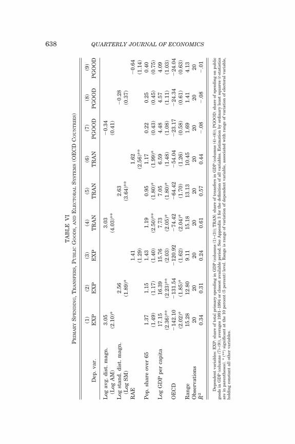
However, Table V hides a substantial difference between thetwo subsamples. Table VI displays the same regressions as TableV for the subsample of OECD countries. In the primary spendingregressions of columns (1)–(3), the coefficients of the electoralvariables are three to five times larger in the OECD subsamplethan in the whole sample, and are now significant at the 10percent level (except for RAE in column (3)). Even stronger re-sults hold for the transfer regressions in columns (4)–(6): now thecoefficients of the electoral variables are typically twice as big asin the corresponding columns of Table V, and all significant atleast at the 2 percent level. The effect of electoral variables ontransfers explains nearly all of their effect on total spending: as aresult, we find small and statistically insignificant negative ef-fects on public good spending (columns (7)–(9)).

Qualitatively, the results for Latin America, displayed inTable VII, are almost the mirror image of those for OECD coun-tries, although they are statistically less strong (we do not displayresults with RAE, because in the Latin American sample we haveonly fifteen observations on this variable). The effect of electoralvariables on total spending is now negative, although statisticallyinsignificant (columns (1)–(3)). This is the result of almost noeffect on transfers (columns (4)–(6)) and a large negative effect onpublic good spending (columns (7)–(9)), although with high p-values, between .15 and .20.

All the point estimates in Tables V to VII are consistent withthe predictions of subsection IV.3. Consistent with Results 1 and2, more proportional systems always have higher transfers andlower public good spending, ceteris paribus. Consistent with Re-sult 3, more proportional systems are associated with higher totalprimary spending, in OECD countries, which have high transferspending, and with lower primary spending in Latin Americancountries, which have low transfers regardless of the electoralsystem.

These results complement those of a related literature thathas studied the difference in Latin American and OECD fiscalpolicy. As documented in Gavin and Perotti [1997], in LatinAmerica most of the fiscal policy response to cyclical variations inthe economy and to external shocks occurs on public good spend-ing, in OECD countries on transfer spending. This paper showsthat the (cross-country) response of fiscal policy to electoral insti-


TA

BL

EV

IP

RIM

AR

YS

PE

ND

ING

,T

RA

NS

FE

RS,

PU

BL

ICG

OO

DS,

AN

DE

LE

CT

OR

AL

SY

ST

EM

S(O

EC

DC

OU

NT

RIE

S)

Dep

.va

r.(1

)E

XP

(2)

EX

P(3

)E

XP

(4)

TR

AN

(5)

TR

AN

(6)

TR

AN

(7)

PG

OO

D(8

)P

GO

OD

(9)

PG

OO

D

Log

avg.

dist

.m

agn

.3.

053.

03�

0.34

(Log

AM

)(2

.10)

*(4

.03)

**(0

.41)

Log

stan

d.di

st.

mag

n.

2.56

2.63

�0.

28(L

ogS

M)

(1.8

9)*

(3.6

4)**

(0.3

7)R

AE

1.41

1.62

�0.

64(1

.29)

(2.5

6)**

(1.1

4)P

op.

shar

eov

er65

1.37

1.15

1.43

1.19

0.95

1.17

0.22

0.25

0.40

(1.4

9)(1

.17)

(1.4

0)(2

.50)

**(1

.80)

*(1

.99)

*(0

.43)

(0.4

5)(0

.75)

Log

GD

Ppe

rca

pita

17.1

516

.39

15.7

67.

737.

056.

594.

484.

574.

09(2

.36)

**(2

.23)

**(2

.03)

(2.0

5)*

(1.8

0)*

(1.4

8)(1

.08)

(1.1

1)(1

.03)

OE

CD

�14

2.10

�13

1.54

�12

0.92

�74

.42

�64

.42

�54

.04

�23

.17

�24

.34

�24

.04

(2.0

2)*

(1.8

5)*

(1.6

2)(2

.04)

*(1

.70)

(1.2

6)(0

.58)

(0.6

1)(0

.63)

Ran

ge15

.28

12.8

09.

1115

.18

13.1

310

.45

1.69

1.41

4.13

Obs

erva

tion

s20

2020

2020

2020

2020

R�2

0.34

0.31

0.24

0.61

0.57

0.44

�.0

8�

.08

�.0

1

Dep

ende

nt

vari

able

s:E

XP

:sh

are

ofto

tal

prim

ary

spen

din

gin

GD

P(c

olu

mn

s(1

)–(3

));T

RA

N:s

har

eof

tran

sfer

sin

GD

P(c

olu

mn

s(4

)–(6

));P

GO

OD

:sh

are

ofsp

endi

ng

onpu

blic

good

sin

GD

P(c

olu

mn

s(7

)–(9

)),a

vera

ges

1991

–199

4or

clos

est

avai

labl

epe

riod

.See

App

endi

x3

for

the

defi

nit

ion

ofal

lva

riab

les.

Est

imat

ion

byor

din

ary

leas

tsq

uar

es(t

-sta

tist

ics

are

inpa

ren

thes

es).

*(*

*)si

gnifi

can

tat

the

10pe

rcen

t(5

perc

ent)

leve

l.R

ange

isra

nge

ofva

riat

ion

ofde

pen

den

tva

riab

le,a

ssoc

iate

dw

ith

ran

geof

vari

atio

nof

elec

tora

lva

riab

le,

hol

din

gco

nst

ant

all

oth

erva

riab

les.


tutions also follows the same pattern: it affects mostly public goodspending in Latin America, and mostly transfer spending inOECD countries.

For Latin America, results are statistically much weaker. Wehave two candidate explanations for this difference—besides theobvious one that our theory fits Latin America less well thanOECD countries. First, measurement error: both the budget vari-ables and the electoral variables are measured less precisely inLatin American countries. Second, Latin America and its fiscalpolicy are subject to larger and more frequent shocks than OECDcountries (see, e.g., Gavin et al. [1996]); hence, it is likely that therole of electoral systems in shaping fiscal outcomes will be harderto detect in Latin America.

VII.4. Robustness

Because of the small sample size, our benchmark specifica-tion is necessarily very parsimonious. Several variables that wehave omitted could conceivably be correlated both with the elec-toral systems and with fiscal outcomes. In Table A2, available

TABLE VIIPRIMARY SPENDING, TRANSFERS, AND ELECTORAL SYSTEMS

(LATIN AMERICAN COUNTRIES)

(1)EXP

(2)EXP

(3)TRAN

(4)TRAN

(5)PGOOD

(6)PGOOD

Log avg. distr. magn. �0.91 0.36 �0.99(Log AM) (0.86) (0.67) (1.31)

Log stand. distr. magn. �1.08 0.14 �0.96(Log SM) (1.13) (0.28) (1.40)

Pop. share over 65 0.69 0.49 0.98 0.95 �0.38 �0.52(0.96) (0.65) (2.69)** (2.44)** (0.75) (0.97)

Log GDP per capita �1.45 �0.77 1.50 1.44 �2.42 �1.83(0.51) (0.27) (1.04) (0.96) (1.20) (0.89)

Constant 29.84 26.00 �12.12 �11.13 37.64 33.87(1.40) (1.24) (1.12) (1.02) (2.49)** (2.26)**

Range 4.38 5.61 1.72 0.71 4.72 4.99Observations 20 20 20 20 20 20R� 2 �.04 0.00 0.40 0.38 0.09 0.10

Dependent variables: EXP: share of total primary spending in GDP (columns (1)–(2)); TRAN: share oftransfers in GDP (columns (3)–(4)); PGOOD: share of spending on public goods in GDP (columns (5)–(6)),averages 1991–1994 or closest available period. See Appendix 3 for the definition of all variables. Estimationby ordinary least squares (t-statistics are in parentheses). * (**) significant at the 10 percent (5 percent) level.Range is range of variation of dependent variable, associated with range of variation of electoral variable,holding constant all other variables.


from the authors at http://www.iue.it/Personal/Perotti web site,we display the estimated coefficients of the electoral variableswhen we add these omitted variables, one at a time, in thespecification estimated so far; we also display the estimated co-efficient of the added variable. In this section we briefly discussthe main results: to conserve space, we focus on the most relevantdependent variables in the two groups of countries: transferspending in OECD countries, and spending on public goods inLatin American countries. Also, we present results for LogSMonly: results with the other variables are similar.

Conventional wisdom has it that proportional systems tendto be associated with a larger number of parties in Parliamentand therefore with larger coalition governments. In turn, empiri-cally larger coalitions tend to be associated with more expendi-ture, particularly on transfers (see Perotti and Kontopoulos[1999]). To address this issue, we add the log of the averageeffective number of parliamentary parties, LogENPP, to the listof independent variables. In OECD countries the estimated coef-ficient of LogENPP is positive, albeit insignificant; more impor-tantly, the coefficient of LogSM remains significant at the 5percent level. In Latin America the estimated coefficient ofLogSM practically does not change.35 Very similar results obtainwhen we use for OECD countries the number of parties in thecoalition, from Perotti and Kontopoulos. We conclude that theelectoral system has an effect on fiscal outcomes independent ofits effects on the degree of party fractionalization both in electionsand in Parliamentary representation.

In an influential paper Rodrik [1998] argues that more opensocieties spend more on government transfers as insuranceagainst external shocks. When we include openness in our regres-sions, its coefficient is always entirely insignificant in both theOECD and Latin American samples; the coefficients of the elec-toral variables are largely unaffected. The same happens if weinteract the openness variable with the volatility of the terms oftrade, as suggested by Rodrik.36

One could also argue that more ethnically or linguistically

35. In a study of the effects of electoral institutions on fiscal performance inLatin America, Stein, Talvi, and Grisanti [1999] find that the only “political”variable correlated with the size of total spending (inclusive of interest payments)is the effective number of parties.

36. These results are potentially important in view of the considerable debatethat Rodrik [1998] has generated. See, for instance, Alesina and Wacziarg [1998,1999].


“fragmented” countries might have more proportional systems, toensure the representation of all minorities; ethnolinguistic frac-tionalization might also independently affect the provision ofpublic goods, for instance as a means to ensure the consensus ofdifferent groups, as in Alesina and Spolaore [1997]. When weinclude ethnolinguistic fractionalization in our regressions, itscoefficient is insignificant, and the coefficient of the electoralvariable is not affected.37

Another potentially relevant omitted variable is ideology.Countries with larger district magnitudes tend to be Nordic coun-tries, with a Social-Democratic tradition, or Southern Europeancountries, that have had leftist governments for long periods oftime. Thus, when we add an ideology variable, IDEOL (not avail-able for Latin American countries), which takes values rangingfrom 1 in more rightist governments to 5 in the more leftist ones(see Appendix 3 for a more detailed description). Its coefficienthas a t-statistic very close to 0, while the estimated coefficient ofthe electoral variable is virtually unchanged.

Particularly in small samples, one has to worry about therobustness of the results to possible outliers. In the OECD group,when we exclude one country at a time, the p-value on theestimated coefficient of the electoral variables in the transferregression never falls below .05.38 In Latin America the initialresults are statistically less strong to begin with; a similar exer-cise confirms that no individual country is responsible for theseweaker results.

One could also worry that the 1991–1994 period might not berepresentative, for instance because it was a period of widespreadfiscal consolidations in many countries. We do not have a choicefor Latin American countries, but for OECD countries we have

37. Alesina, Baqir, and Easterly [1999] find that in ethnically fragmentedU. S. cities the provision of public goods is lower, while Ordeshook and Shvestova[1994] present cross-country evidence on the impact of ethnic fractionalization onthe effective number of parties under different electoral systems.

38. In principle, two countries could have a nontrivial influence on the re-sults: the Netherlands, with a very large average district magnitude (its propor-tional system consists of only one district electing 150 representatives) andFrance, the only non-English speaking country with a majority system, but at thesame time with a very high share of transfers in GDP, close to 30 percent. Indeed,when we reestimate all our regressions dropping one country at a time, wetypically find that the exclusion of France causes the estimated coefficients ofelectoral variables and their t-statistics to increase dramatically; the exclusion ofthe Netherlands causes them to fall somewhat, although they always remainsignificant at the 5 percent level. When we exclude both countries, point estimatesand t-statistics rise considerably relative to the benchmark regressions of Table VI.


annual data over the whole 1960–1995 period. When we reesti-mate the regressions of Table VI using cross-sectional data basedon 1960–1995 averages, we find even stronger results, withlarger and more significant coefficients in the total spending andtransfer regressions.

VIII. TIME-SERIES EVIDENCE: INTERACTIVE EFFECTS

In the OECD sample we can exploit the time dimension of thefiscal data to investigate the following question: do electoral in-stitutions affect the response of fiscal variables to shocks? Thespirit of the model suggests that the increase in governmentspending in response to a given shock should be higher in a moreproportional system.39 Except for RAE, the electoral measures weuse in the previous regressions display limited or no time varia-tion in the OECD sample;40 hence, it does not make sense to runpure fixed effects panel regressions, because the fixed effects andthe electoral variables would be highly collinear. We use twodifferent methodologies, designed to estimate the responses tocommon shocks and to country-specific shocks, respectively.

VIII.1. Common Shocks

To study the response to common shocks, we borrow themethodology of Blanchard and Wolfers [2000]: we estimate re-gressions of the type,

(16) Git � ci � dt�1 � �Xi� � �POP65it � �LogGDPPCit � �it,

where i indexes the country and t the period. ci is a country-specific intercept, dt is a time dummy, and the other variableshave been defined previously. Thus, in this specification the timedummies capture the common shocks, and their effects depend onthe value of the electoral variable. This dependence is captured bythe coefficient �.

Without a richer dynamic specification (which would be dif-ficult to estimate given the short time series) it would not be

39. Strictly speaking, this question is outside the model. However, it couldeasily be incorporated in a version of the model where the current policy acts asthe status quo.

40. There is more time series variation in the Latin American sample, due tothe frequent changes in electoral laws engendered by new administrations. How-ever, it is extremely difficult to reconstruct precisely electoral laws further backthan the early nineties, and in many countries meaningful democratic electionsbegan only in the mid- or late eighties.


reasonable to interpret this regression as capturing the effects ofelectoral institutions on year-to-year changes in fiscal policy:hence, all our variables are averages over a five-year period, andthe time index t refers to five-year periods, beginning in 1960 orthe earliest available year.

Table VIII reports estimates of equation (16) (by nonlinearleast squares) on the sample of twenty OECD countries, with thespending/GDP ratio (columns (1)–(3)) and the transfer/GDP ratio(columns (4)–(6)) as the dependent variables.41 In the case ofRAE, which has meaningful time series variation, the regressionalso includes the variable by itself. The first row of Table VIIIdisplays the effects of the “pure” time effects, i.e., the increase inthe spending/GDP ratio that would have been experienced by a

41. The presentation of results also follows Blanchard and Wolfers [2000].

TABLE VIIICOMMON SHOCKS AND ELECTORAL SYSTEMS

PANEL REGRESSIONS, INDUSTRIAL COUNTRIES

Dep. var.(1)

EXP(2)

EXP(3)

EXP(4)

TRAN(5)

TRAN(6)

TRAN

Time 14.91 14.02 14.29 13.19 12.78 12.40Log AM � time dummy 0.10 0.13

(2.08)** (4.93)**Log SM � time dummy 0.07 0.11

(1.61) (4.35)**RAE � time dummy 0.05 0.06

(1.84)* (3.56)**RAE �2.95 �2.93

(�1.43) (�2.79)**Pop. share over 65 0.95 1.01 0.95 0.21 0.21 0.25

(2.22)** (2.43)** (2.28)** (1.08) (1.06) (1.23)Log GDP per cap. �4.09 �3.62 �3.84 �4.79 �4.46 �4.43

(�1.17) (�1.04) (�1.08) (�2.94)** (�2.68) (�2.53)**Min 0.82 0.86 0.68 0.78 0.80 0.64Max 1.34 1.22 1.12 1.43 1.32 1.14Range 0.52 0.36 0.44 0.65 0.52 0.50Observations 112 112 112 112 112 112R� 2 0.92 0.92 0.91 0.96 0.96 0.96

Dependent variable: share of total primary spending in GDP (columns (1)–(3)) and share of transfers inGDP (columns (4)–(6)); five-year averages from 1960 (earliest available year) to 1995. See Appendix 3 for thedefinition of all variables. Estimation by nonlinear least squares (t-statistics are in parentheses). * (**)indicates statistical significance at the 10 percent (5 percent) level. Range is range of variation of dependentvariable, associated with range of variation of electoral variable, holding constant all other variables(minimum and maximum values also reported).


country with the average value of the electoral variable. Thus, thepure time effect is equal to the difference between the estimatedtime effects in 1990–1995 (the last one) and 1960–1964. The nextrow reports the estimate of � with its t-statistic. The rows labeled“Min” and “Max” answer the following question: suppose that acommon shock causes the spending/GDP ratio to increase by 1percentage point in the country with average values of the elec-toral variable: by how much does the spending/GDP ratio in-crease in the countries with the lowest and highest values of theelectoral variable? The answer is given by 1 �Xmin and 1 �Xmax, respectively. The row labeled “Range” displays the differ-ence between the two.

Table VIII provides some support for the notion that inresponse to common shocks primary spending increases by morein more proportional systems than in other systems, and muchstronger support for the notion that transfers increase by more inmore proportional systems. In the primary spending regressions,all the estimates of � are positive, and significant in the case ofLogAM (at the 5 percent level) and RAE (at the 10 percent level).According to the point estimates, the range of variation in thespending/GDP ratio in response to a shock that causes the sameratio to increase by 1 percentage point in the “average” country, isbetween .36 and .52 percentage points of GDP.

In the transfers regressions (columns (4)–(6)) the coefficientsof the electoral variables are very close to those in the spendingregressions, and the t-statistics are much higher—the p-valuesare all below .001. The implied range of variation in the transfer/GDP ratio in response to the “average” shock is even larger, from.5 to .65 percentage points of GDP. Note also that the “pure” timeeffect (first row) is similar across all columns.

VIII.2. Country-Specific Shocks

We now allow electoral institutions to interact with country-specific shocks. To do so, we need a macroeconomic shock whoseeffects on spending are a priori clear. An increase in unemploy-ment will cause most types of government spending to increaserelative to GDP, both because of the working of automatic stabi-lizers and because of the discretionary response by the govern-ment. Thus, we estimate regressions of the type,

(17)

Git � ci � dt � �Uit � �UitXi � �POP65it � �LogGDPPCit � �it.


Uit is the unemployment rate in country i in period t. Thus, �captures the interaction of a shock to unemployment with theelectoral system: if a country with a more proportional systemresponds to a shock to unemployment by increasing spending ortransfers more, � is positive. As before, because RAE displaysmeaningful time series variation, we also include the variable byitself, in addition to its interaction with U.

Table IX displays the results. The estimated coefficient of Uis indeed always positive and significant: over a five-year horizon,in a majority system (where LogAM and LogSM are equal to 0) anincrease in unemployment by 1 percentage point is associatedwith an increase in the total primary spending/GDP ratio bybetween .42 and .48 percentage points, and an increase in thetransfers/GDP ratio by between .27 and .31 percentage points.

The estimates of the interactive term coefficient, �, are al-ways positive, but they are significant at the 5 percent level onlywhen transfers/GDP is the dependent variable (columns (4)–(6)).

TABLE IXCOUNTRY-SPECIFIC SHOCKS AND ELECTORAL SYSTEMS

PANEL REGRESSIONS, INDUSTRIAL COUNTRIES

Dep. var.(1)

EXP(2)

EXP(3)

EXP(4)

TRAN(5)

TRAN(6)

TRAN

Log AM � unempl. rate 0.14 0.15(1.60) (3.15)**

Log SM � unempl. rate 0.09 0.11(1.25) (2.80)**

RAE �0.14 �0.39(�0.30) (�1.53)

RAE � unempl. rate 0.05 0.06(1.01) (2.09)**

Unempl. rate 0.42 0.48 0.8 0.27 0.30 0.68(2.04)** (2.38)** (4.44)** (2.38)** (2.74)** (6.80)**

Pop. share over 65 1.68 1.68 1.77 1.05 1.04 1.15(4.38)** (4.35)** (4.58)** (5.00)** (4.91)** (5.31)**

Log GDP per capita 4.59 4.46 3.94 2.69 2.62 2.17(1.90)* (1.84)* (1.62) (2.04)** (1.97)** (1.60)

Range 0.72 0.47 0.46 0.77 0.57 0.53Observations 112 112 112 112 112 112R� 2 0.90 0.90 0.90 0.94 0.94 0.94

Dependent variable: share of total primary spending in GDP (columns (1)–(4)) and share of transfers inGDP (columns (5)–(8)); five-year averages from 1960 (earliest available year) to 1995. See Appendix 3 for thedefinition of all variables. Estimation by nonlinear least squares (t-statistics are in parentheses). * (**)indicates statistical significance at the 10 percent (5 percent) level. Range is range of variation of dependentvariable, associated with range of variation of electoral variable, holding constant all other variables(minimum and maximum values also reported).


The implied economic significance is also considerable: from therow labeled “range,” a 1 percentage point shock to unemploymentcauses the transfers/GDP ratio to increase by between .53 and .77percentage points more in the most proportional electoral systemthan in the least proportional one.

Both types of panel regressions are robust to outliers. Wereestimated all regressions in Tables VIII and IX dropping onecountry at a time, and both France and the Netherlands at thesame time. The estimates of � change only minimally, and so dotheir p-values.

IX. RELATION WITH THE LITERATURE

We now discuss the relationship between our contributionand the existing literature, in terms of both theory and empirics.In Persson and Tabellini [1999a, 2000, 2001] two candidatesmake binding promises on the provision of a “universal” type ofspending, and on a “targetable” one (which is both district- andgroup-specific). The driving force is uncertainty by the policymak-ers over the distribution of voters’ preferences, and therefore overthe identity of the median voter. In a majoritarian system thecandidates compete for “swing” districts, by directing the tar-getable instrument toward a narrower constituency, identified intheir model with the “middle class.” Hence, majoritarian systemshave higher spending on the more targetable instrument, and alower provision of the universal public good. By focusing on votersin a limited number of districts, politicians in a majoritariansystem fail to internalize the overall distortions induced by tax-ation decisions, thus also leading to a larger government.

Thus, in terms of the composition of spending, these modelspredict that the universal type of spending will be higher inproportional systems, while the targetable type of spending willbe higher in majoritarian systems; in terms of the level of spend-ing, the prediction is that total government expenditure will behigher in majoritarian systems. In contrast, our model predictsthat expenditure on transfers will be higher in proportional sys-tems, while expenditure on purchases of goods and services willbe higher in majoritarian systems; the effect of the electoralsystem on total government spending depends on the share of


transfers in total spending—and, more deeply, the underlyingdistribution of voters preferences.42

In estimating these models, Persson and Tabellini mostlycapture the properties of the electoral system via a “majoritarian”dummy variable.43 In Persson and Tabellini [1999a] public goodsare the universal expenditure and transfers the targetable one. Inthe empirical application, the universal public good is definedmore specifically as expenditure on order and safety, health,transportation, and education; in a cross section of 50 countries,there is evidence that expenditure on these universal public goodsis indeed higher in proportional systems, and that total govern-ment expenditure is higher in majoritarian systems. In Perssonand Tabellini [2000, 2001] welfare transfers are instead the uni-versal expenditure, and local public goods are the targetable one.In the empirical application they find, based on a panel of 60countries, that majoritarian systems tend to have lower overallexpenditure and especially lower welfare spending.44

Another difference with our approach is that our theory andour empirical results underscore the importance of disaggregat-ing the sample: the relation between degree of proportionalityand size of transfers is positive and very robust among OECDcountries, but not so for Latin American countries.

X. CONCLUDING REMARKS

In this paper we have studied the effects of electoral institu-tions on the size and composition of public expenditure in OECDand Latin American countries. We have emphasized the distinc-tion between purchases of goods and services, which are easier to

42. In Lizzeri and Persico [2001] two candidates make binding promises onthe level of spending on two types of government expenditure, a universal publicgood and transfers that can be targeted geographically or by groups. Even whenthe public good is more valuable to individuals, in a majoritarian system, wherethe spoils of office go to the winner, on average one could have lower provision ofthe universal public good.

43. For some regressions, Persson and Tabellini [1999a] also use the inverseof the average district magnitude, from Cox [1997]. However, the construction ofthis variable does not take into account the specific features of two-tier systemsthat we highlighted in Sections V and VI.

44. However, the main focus of these papers is on the dichotomy betweenpresidential and parliamentary systems; in this case, Persson and Tabelliniconsistently find that presidential systems tend to have lower government expen-diture. In an interesting study at a more disaggregated level, Baqir [2001] findsthat in a cross section of U. S. cities larger district councils are associated withlarger city governments, and that spending is higher when councils are elected “atlarge” than when they are elected by city district.


target geographically, and transfers, which are easier to targetacross social groups. We presented a theoretical model in whichvoters anticipating government policymaking under differentelectoral systems have an incentive to elect representatives moreprone to transfer (public good) spending in proportional (majori-tarian) systems. The model also predicts higher total primaryspending in proportional (majoritarian) systems when the shareof transfer spending is high (low).

To test our predictions, we have defined and constructedrigorous measures of proportionality that take into account theexistence of different voting methods, multiple electoral tiers, andelectoral thresholds. In the empirical investigation, we havefound strong support for our predictions in OECD countries, andmuch weaker evidence for Latin American countries. Interest-ingly, the positive relation between transfers and the degree ofproportionality in OECD countries holds even within propor-tional systems, highlighting the importance of constructing mea-sures of proportionality that go beyond the majoritarian/propor-tional dichotomy. In future research it would be interesting toexamine the relation between electoral systems and the distribu-tion of expenditure within countries, since existing models (in-cluding ours) have strong implications in this regard.

APPENDIX 1

Given the assumption of uniform distribution of preferences(�,�) over the rectangle with vertices �L,�H,�L,�H, the voter withmedian preferences over � and � is the decisive voter in eachelectoral system. This result would still hold if we relaxed theassumption about uniform distribution of preferences, as long asthese are nondegenerate and bounded, and allowed the represen-tative to be selected by a sequential vote on � and �, regardless ofthe order of voting.

Consider the majoritarian system first, and suppose initiallythat the sequencing on votes is first on � and then on �. Considerthe problem solved by individual i of group B in district k1 (forbrevity, we will omit the subscript B to indicate the group whenthis does not create any ambiguity). Starting from the secondstage, let �*k1

denote the value of � that has prevailed by majorityvoting in the first stage. The problem of individual i in district k1is to find the optimal value of � for a representative who alreadyhas a value of � equal to �*k1

. Denote this optimal value of � from


the perspective of individual i by �*ik1. This is found by maximiz-

ing with respect to �*k1expression (5) (with the index i replacing

the median voter index m), subject to tM, s�BM, and g1

M being givenby suitable modifications of expressions (4), and taking as given�*k1

, �*k2, �*k3

, �*k2, and �*k3

. It is easy to see that one obtains�*ik1

� �ik1. Thus, in the second stage an individual with median

value of � prevails in each district.In the first stage, the optimal value of � for a representative

from the point of view of individual i in district k1, �*ik1, is found

by maximizing the same expression above with respect to �ik1,

with �*k1� �m. Again, it is easy to see that one obtains �*ik1

��ik1

/(2 � �ik1). Hence, the individual with median value of � is

decisive in the first stage.A similar reasoning applies when voting first on �, then on �,

and in the proportional system.

APPENDIX 2

As we mentioned in the text, in two-tier electoral systemsthere is a distinction between the upper bound on the number ofrepresentatives that can be elected in a district and the actualnumber of representatives that can be elected. We denote with anasterisk actual sizes: thus, S*ik denotes the actual district size ofdistrict k in tier i, and analogous definitions hold for S*i and S� *i:note that for T2 districts, S2k � S*2k always; i.e., they are alwaysconditional on T1 results. Clearly, S*2 � 0 for one-tier systems.

In Remainder Seats systems, S2 is variable: in principle, allor no seats could be attributed in T1 (S1 � Stot); but typicallyonly some are (S*1 � S1), and the remainder seats are filled in T2(S2 � S*2 � Stot � S*1). In Adjustment Seats systems, S2 is fixed;hence, S*1 � S1, and S2 � S*2 � Stot � S1.

2.1. Local Requirements

A first type of local requirement sets a minimum share ofvotes that a party must obtain in a given district in order toparticipate in the allocation of seats in that district; this is equiva-lent to a legal threshold of the same size applying to that tier. Asecond type of local requirement defines a fraction h of an upperquota that a party must win in at least one district in T1 in orderto have access to the allocation of seats in T2. To translate thisrequirement into a legal threshold, note that the binding con-straint is meeting the requirement in the largest district of T1.


Hence, the legal threshold in T2 is THR2 � hQ1 (S1max). We haveassembled information on the maximum district size in T1, andwe use it in constructing THR2 whenever the local requirement isof this type.

2.2. Upper Quotas

We now provide the formulas for the upper quota in thedifferent voting methods and formulas. In all cases, we will referto “party A” as the party whose share is equal to the upper quota.We will assume that there are P parties in each district.

Majority/Plurality Methods

FPTP: clearly Qi(Sik) � .5Alternative Vote: Qi(Sik) � .5Two-Round: Qi(Sik) � .5

Largest Remainder Methods

In LR methods in which “remainders” are transferred to anupper tier, the formulas for the upper quotas are clearly the sameas the quotas themselves: any party needs to reach the full quotato be assured of a seat. The exception is the LR Imperiali method,where the number of quotas can exceed the number of seats.Hence,Hare: Qi(Sik) � 1/SikDroop: Qi(Sik) � 1/(1 Sik)45

Imperiali: Qi(Sik) � 1/(1 Sik).In LR methods in which remainder seats are attributed

within the same electoral tier, the formulas for the Droop andImperiali quotas are unchanged. For the Hare quota, instead,they depend on the relation between the number of seats in thedistrict and the number of parties P competing for the seats (seeLijphart and Gibberd [1977] and Gallagher [1991]). If Sik P,the upper quota is 1/(1 Sik), as for the other methods. If Sik �P, the upper quota is (P � 1)/PSik for the Hare formula.

45. In the Japanese SNTV method, the share that guarantees a candidateelection without resorting to any second-round allocation of votes is defined by lawas the Droop quota, hence Qi(Sik) � 1/(1 Sik). For the purpose of calculatingupper quotas, we consider the Irish STV method as equivalent to a Droop formula.In fact, the Irish system establishes that the Droop quota guarantees election fora candidate. We assume that this is also the quota for a party. Hence, Qi(Sik) �1/(1 Sik).


Highest Average Methods

d’Hondt. The least favorable distribution of votes for party Ais when another party (say party P) gets all the remaining votes.Party A still gets one seat if party P gets a vote share VP which isjust short of VASik. Thus, when the vote share of the two partiesare divided by 1,2, . . . , Sik � 1, party P gets a seat each time.The last quotient, VP/Sik, is (infinitesimally) smaller than VA,hence party A gets the last representatives. Hence, Qi(Sik) isdefined by the conditions

VA � VP � 1; VA � VP/Sik; Qi�Sik� � VA,

which gives Qi(Sik) � 1/(1 Sik). This formula is valid irrespec-tive of the relation between number of parties and number ofseats.

Modified St. Lague. We present the conditions for the Modi-fied St. Lague formula, since this is always used instead of thepure St. Lague formula. Under Modified St. Lague, the partyshares are divided by 1.4,3,5, . . . instead than by 1,3,5, . . . In thiscase we need to distinguish between the case in which the num-ber of parties is larger than the number of seats (Sik P) and theopposite case. In the former case, the worst distribution of votesfor party A obtains when Sik other parties get a share of voteswhich is the same as the share of party A. This implies that thevote share to ensure election is implicitly given by VA/1.4 � (1 �VA)/1.4Sik, which in turn implies Qi(Sik) � 1/(1 Sik). Ifinstead the number of parties is “intermediate” (Sik � P �Sik/ 2 1), then Qi(Sik) � 1.4/(1.6 Sik � 0.2P 1.6) [Gal-lagher 1992]. Finally, if the number of parties is “small” (P (Sik/ 2 1), then Qi(Sik) � 1.4/(2Sik � P 2.4) [Lijphart andGibberd 1977].

2.3. Calculation of Upper Marginal Share in Two-Tier RVSystems

In this Appendix we show the calculation for the case when aLargest Remainder method is used in T1. In our sample, onlyNorway after 1990 uses a Highest Average method to attributeT1 seats. The eight T2 seats are attributed to the T1 district listswith the eight highest averages after the averages that earned aseat. Unlike in a Largest Remainder method, in a Highest Aver-age method a seat can be attributed in T1 even to a party thatgets less than the upper quota. Therefore, it is more difficult to


approximate the share of votes that go to T2 as remainders, andto calculate UMS2. However, because the number allocated in T2seats is less than 5 percent of the assembly size, by the rule we setout above we do not consider T2 in this case. In any case, becauseT2 is so small, we know that UMS2 must be very close to UMS1.This leaves Austria and Italy 1960–1993 to represent two-tier RVsystems. Seats are attributed in a T1 district only if the upperquota is met,46 hence on average each seat attributed in T1 usesa fraction of district votes equal to Q1(S� 1), (assuming, as it isalways the case in practice, that this is larger than THR1; seesubsection V.3), and a fraction of national votes equal to Q1(S� 1)/D1.47 A total of S*1 seats are attributed in T1 this way, thusleaving a fraction 1 � S*1Q1(S� 1)/D1 of national votes to be usedfor the allocation of the remaining S2 T2 seats.48 Assuming thatall T2 districts have the same size, and ignoring for the momentlegal thresholds, to be guaranteed a seat in a T2 district a partyneeds a share Q2(S� 2) of all the average T2 district votes, hencethe same fraction of all T2 votes, hence a fraction Q2(S� 2)(1 �S*1Q1(S� 1)/D1) of national votes. UMS2 can then be computed asUMS2 � max (Q2(S� 2)(1 � S*1Q1(S� 1)/D1), THR2).

APPENDIX 3

3.1. List of Countries

OECD countries: Australia, Austria, Belgium, Canada, Den-mark, Finland, France, Germany, Greece, Ireland, Italy, Japan,Netherlands, Norway, Portugal, Spain, Sweden, Switzerland,United Kingdom, United States.

Latin American countries: (all variables are taken as averagesover the 1991–1994 period, unless otherwise indicated): Argentina,Bolivia (1993–1994), Brazil (1991–1992), Chile, Colombia (1992–1993), Costa Rica, Dominican Republic, Ecuador, El Salvador, Gua-

46. Recall that, when a Largest Remainder method is used in T1 districts ofRV systems, Q1(S1k) is the actual share of district votes used for each seatallocated in district k of T1.

47. This is clearly an approximation because we replace the average ofQ1(S1k) with Q1(S� 1).

48. We do not have information on S*1 for each election; however, Taageperaand Shugart [1989] do provide information on the average value of S*1, where theaverage is taken across elections in a given country. In the empirical implemen-tation of our variables, we use this average value as a proxy for the actual valueof S*1. Throughout these calculations, we assume that there are no abstentions orinvalid ballots.


temala, Honduras, Jamaica (1993–1994), Mexico, Nicaragua (1992–1994), Panama (1991–1993), Paraguay (1993–1994), Peru (1990–1991), Trinidad and Tobago (1992–1994), Uruguay (1991–1992),Venezuela.

3.2 Fiscal Variables

OECD Countries

All fiscal variables are from the OECD Economic OutlookDatabase, and refer to the general government.

TRAN Transfers to households. Defined as SSPG TRPGusing the mnemonics of the Economic Outlook Data-base. SSPG: Social security benefits to households;TRPG: Other transfers to households.

PGOOD Public goods, defined as the sum of government consump-tion and government investment, net of depreciation:CGW CGNW CAPEXP. CGW: Government con-sumption, wages; CGNW: Government consumption, ex-cluding wages; CAPEXP: government investment, net ofdepreciation, plus net capital transfers paid.

EXP Total primary government expenditure, defined asTRAN PGOOD residual item, where residual item �TSUB YPEPG � GNINTP. TSUB: Subsidies to firms;YPEPG: Property income paid by government; GNINTP:Net interest payments by government.

Latin American Countries

For Argentina, Bolivia, Brazil, Chile, Colombia, Costa Rica,Ecuador, Mexico, Panama, Paraguay, Peru, Uruguay, Venezuela:Gavin and Perotti [1997], based on IMF data, World Bank data,and national data. For Dominican Republic, El Salvador, Guate-mala, Honduras, Jamaica, Nicaragua, Trinidad and Tobago: IMFdata.

All definitions are consistent, and follow the IMF Govern-ment Financial Statistics classification, which in turn is, for largeaggregates, virtually identical to the OECD Economic Outlookclassification.


3.3. Political Variables

Log AM Logarithm of average district magnitude. AM is de-fined as the weighted average of the average districtsizes of the two electoral tiers, with weights equal tothe proportion of all representatives elected in thetwo tiers (see Section VI for details). Sources: forOECD countries authors’ calculations based on Ta-agepera and Shugart [1989], Lijphart [1994], andnational sources, for Latin American countries Inter-Parliamentary Union (various years), Political data-base of the Americas (http://www.georgetown.edu/pdba/english.html), and national sources (mostlyconstitutions and electoral laws in place at the timeswe take our cross-sectional observations).

Log SM Logarithm of Standardized Average District Magni-tude. SM is defined as 1/UMS � 1, where UMS is theminimum share of national votes which guarantees aParliamentary seat to a party (see Section VI for de-tails). Sources: for OECD countries authors’ calcula-tions based on Taagepera and Shugart [1989], Lijphart[1994], and national sources, for Latin American coun-tries Inter-Parliamentary Union (various years), Politi-cal database of the Americas, and national sources.

LogENPP Logarithm of the effective number of Parliamentaryparties. ENPP is defined as ¥p/sp

21, where sp is the shareof seats of party p. Source: for OECD countries Lijphart[1994] and unpublished data from Lijphart extended tothe early 1990s using national sources; for Latin Ameri-can countries Inter-Parliamentary Union (variousyears), Political database of the Americas, and nationalsources.

IDEOL Ideological configuration of government. The variabletakes values from 1 (dominant right-wing party) to 5(dominant left-wing party). Source: Woldendorp, Ke-man, and Budge [1993] and updates from Perotti andKontopoulos [1999] (available only for OECD countries).


MAJ Dummy variable taking the value of one if the elec-toral system is majoritarian and zero otherwise.Source: Persson and Tabellini [1999a].

MAGN Effective district magnitude. Source: Taagepera andShugart [1989], Lijphart [1994] and authors’ exten-sions (until 1995).

3.4. Other Variables

ETHNIC Index of ethnolinguistic fractionalization for 1960.It measures the probability that two randomly se-lected people from a given country will not belong tothe same ethnolinguistic group. Source: Atlas Nar-odov Mira [1964] as reported in Easterly and Le-vine [1997].

LogGDPPC Log of real GDP per capita in thousands of 1985international dollars. Source: Summers and Heston[1991] and Penn World Tables 5.6 update; updatedfor the years after 1992 using World Bank data.

OPEN Ratio of exports of goods and services plus importsof goods and services over two times GDP. Source:World Bank, World Development Indicators andPenn World Tables 5.6 update.

POP65 Ratio of population above 65 to total population.Source: World Bank, World Development Indicators.

U Unemployment rate. Source: OECD Economic Out-look Database.

INTERNATIONAL MONETARY FUND AND CENTRE FOR ECONOMIC POLICY RESEARCH

EUROPEAN UNIVERSITY INSTITUTE AND CENTRE FOR ECONOMIC POLICY RESEARCH

EUROPEAN CENTRAL BANK

REFERENCES

Alesina, Alberto, Reza Baqir, and William Easterly, “Public Goods and EthnicDivisions,” Quarterly Journal of Economics, CXIV (1999), 1243–1284.

Alesina, Alberto, and Enrico Spolaore, “On the Number and Size of Nations,”Quarterly Journal of Economics, CXII (1997), 1027–1056.


Alesina, Alberto, and Romain Wacziarg, “Openness, Country Size, and Govern-ment,” Journal of Public Economics, LXIX (1998), 305–321.

Alesina, Alberto, and Romain Wacziarg, “Is Europe Going Too Far?” Carnegie-Rochester Conference Series on Public Policy, LI (1999), 1–42.

Austen-Smith, David, and Jeffrey Banks, “Elections, Coalitions and LegislativeOutcomes,” American Political Science Review, LXXXII (1988), 405–422.

Baqir, Reza, “Districting and Government Overspending,” IMF Working Paper01/96, August 2001, Journal of Political Economy, forthcoming.

Baron, David P., and Daniel Diermeier, “Elections, Governments, and Parlia-ments in Proportional Representation Systems,” Quarterly Journal of Eco-nomics, CXVI (2001) 933–968.

Besley, Timothy, and Stephen Coate, “Centralized versus Decentralized Provisionof Local Public Goods: A Political Economy Analysis,” NBER Working PaperNo. 7084, 1999.

Blanchard, Olivier Jean, and Justin Wolfers, “The Role of Shocks and Institutionsin the Rise of European Unemployment: The Aggregate Evidence,” EconomicJournal, CX (2000), C1–33.

Chari, V. V., Larry E. Jones, and Ramon Marimon, “On the Economics of Split-Ticket Voting in Representative Democracies,” American Economic Review,LXXXVII (1997), 957–976.

Cox, Gary W., Making Votes Count (New York, NY: Cambridge University Press,1997).

Easterly, William, and Ross Levine, “Africa’s Growth Tragedy: Policies and EthnicDivisions,” Quarterly Journal of Economics, CXII (1997), 1203–1250.

Gallagher, Michael, “Proportionality, Disproportionality and Electoral Systems,”Electoral Studies, X (1991), 33–51.

Gavin, Michael, Ricardo Hausmann, Roberto Perotti, and Ernesto Talvi, “Manag-ing Fiscal Policy in Latin America and the Caribbean: Volatility, Procyclical-ity, and Limited Creditworthiness,” IADB Working Paper No. 326, 1996.

Gavin, Michael, and Roberto Perotti, “Fiscal Policy in Latin America,” NBERMacroeconomics Annual, Ben Bernanke and Julio Rotemberg, eds. (Cam-bridge, MA: MIT Press, 1997).

Inter-Parliamentary Union, Chronicle of Parliamentary Elections and Develop-ments, Geneva, Switzerland (various years).

Lijphart, Arend, Electoral Systems and Party Systems (Oxford, UK: Oxford Uni-versity Press, 1994).

Lizzeri, Alessandro, and Nicola Persico, “The Provision of Public Goods underAlternative Electoral Incentives,” American Economic Review, XCI (2001),225–239.

Milesi-Ferretti, Gian Maria, and Roberto Perotti, with Massimo Rostagno, “Elec-toral Rules and Public Spending,” Centre for Economic Policy Research Dis-cussion Paper No. 2742, March 2001.

Ordeshook, Peter C., and Olga V. Shvestova, “Ethnic Heterogeneity, DistrictMagnitude, and the Number of Parties,” American Journal of Political Sci-ence, XXXVIII (1994), 100–123.

Perotti, Roberto, and Yianos Kontopoulos, “Fragmented Fiscal Policy,” mimeo,Columbia University, (1999) Journal of Public Economics, forthcoming.

Persson, Torsten, and Guido Tabellini, “The Size and Scope of Government:Comparative Politics with Rational Politicians,” European Economic Review,XLIII (1999a), 699–735.

Persson, Torsten, and Guido Tabellini, “Political Economics and Public Finance,”NBER Working Paper No. 7097, 1999b, in Handbook of Public Economics,Vol. 3, Alan Auerbach and Martin Feldstein, eds. (Amsterdam, The Nether-lands: Elsevier Science Publishers), forthcoming.

Persson, Torsten, and Guido Tabellini, Political Economics (Cambridge, MA: MITPress, 2000).

Persson, Torsten, and Guido Tabellini, “Political Institutions and Policy Out-comes: What Are the Stylized Facts?” CEPR Discussion Paper No. 2872, June2001.

Rae, Douglas W., The Political Consequences of Electoral Laws (New Haven, CT:Yale University Press, 1967).


Rodrik, Dani, “Why Do More Open Economies Have Bigger Governments?” Jour-nal of Political Economy, CVI (1998), 997–1032.

Stein, Ernesto, Ernesto Talvi, and Alejandro Grisanti, “Institutional Arrange-ments and Fiscal Performance: The Latin American Experience,” in FiscalInstitutions and Fiscal Performance, James Poterba and Jurgen von Hagen,eds. (Chicago, IL: University of Chicago Press for NBER, 1999).

Summers, Robert, and Alan Heston, “Penn World Tables Mark 5: An ExpandedSet of International Comparisons,” Quarterly Journal of Economics, CVI(1991), 327–368.

Taagepera, Rein, and Matthew Soberg Shugart, Seats and Votes (New Haven, CT:Yale University Press, 1989).

Woldendorp, J., H. Keman, and I. Budge, “A Compilation of Political Data onIndustrialized Parliamentary Democracies,” European Journal of PoliticalResearch, XXV (1993), 1–120.


electoral systems and public spending* in modern democracies, elected

Documents