electrical axes of tesla-type cavities - desy - flash ... · electrical axes of tesla-type cavities...

- 1 -

Electrical axes of TESLA-type cavities (Theoretical background, development of measurement equipment, measurement results)

Anton Labanc, MHF-SL, DESY, January 2008

Abstract

Cells in TESLA cavities after the fabrication are detuned and strongly misaligned. Before cavities are installed into a cryomodule the cells must be aligned and their resonance frequencies must be corrected to obtain equal field amplitudes of the accelerating TM010-π mode in all cells. Until now, the eccentricity (misalignment) of cells is measured mechanically. The mechanical measurement is weakly related to the real electromagnetic fields, both of the accelerating mode and higher order modes. A new method of electromagnetic field mapping inside a cavity based on small perturbation method was developed to improve the axis determination. A short overview was already published at the TESLA Report 2007-01. This paper brings more details about the method, technical background and more measurement results. It contains a lot of fundamentals and basic theory which for many readers is well known since many years, but I hope it will be helpful for novices in this field.

TESLA Report 2008-01

- 2 -

1. Introduction The International Technology Recommendation Panel in August 2004 recommended

implementation of the superconducting (TESLA) technology for the International Linear Collider (ILC) project. Since then many R&D programs have been initialized with a hope to lower the total cost of the ILC main accelerator and improve its performance. The preservation of the colliding beams quality, their low emittance and low energy spread, along the main accelerator is one of the precautions needed for the proper performance of the ILC facility. The dilution of the beam quality is caused by an interaction of the beam with cavity parasitic modes and/or by tilt of a cavity making the accelerating field unparallel to the beam trajectory. Therefore it is of great importance to determine the electrical axis of a cavity, a position which minimizes the dilution.

The tuning method used until now allows minimizing the after fabrication mechanical eccentricity below 0.4 mm. The mechanical measurement has always systematic errors. One source of the error is the non-uniform thickness of the cavity wall after forming the cells by deep-drawing. This measurement can be performed only on the outer surface of the cavity wall and the unknown wall thickness does not allow determination of the actual cavity inner contour. Another error source is that the measurement is done only on equators. If an iris or a side of any cell is deformed, this method cannot detect it.

The small perturbation method measures the field directly and thus makes possible to investigate almost all modes which do not propagate in the beam pipes. Several measured modes provide data sufficient to reconstruct the deformation of cells. If the cell is perfectly rotation-symmetric, all modes have the same electrical axis. Otherwise diverse modes due to their different field patterns are perturbed in different way, which results in different geometrical locations of their electrical axes.

For the electrical axis measurement a special experimental setup was designed and built. After development the setup was tested and used for several 9-cell niobium TESLA cavities and their 9-cell copper model. The expected measurement precision was 0.1 mm in rectangular coordinates (0.14 mm in polar coordinates). Results for the copper model and one niobium cavity are included in this report. The results for the other niobium cavities are very close to the result for niobium cavity presented here.

Fig. 1.1 TESLA cavity


- 3 -

2. Small perturbation theory

2.1. Fundamental equation

The resonant frequency of a mode varies over a certain range when a small perturbing object, e.g. metallic or dielectric sphere, needle, disk or torus etc., is inserted into the cavity interior. The change of the resonant frequency can be found analytically by means of the first and second Maxwell’s equations applied to the unperturbed and perturbed cavity [1, 2]. The other way to find the frequency change is to treat the perturbing object as an electric or magnetic dipole [3]. In the following analysis we will assume that the cavity volume V is filled with ε = 1 medium (vacuum). Further we assume that the resonant mode under consideration has resonant frequency ω0 and amplitudes of the electric and magnetic field E0 and H0 respectively. The inserted perturbing object changes locally the absolute permittivity and permeability by Δε and Δμ. The new resonant frequency ω is then given by:

( )( )∫

∫⋅⋅+⋅

⋅⋅Δ+⋅Δ−=

−∗∗

∗∗

V

V

dVHHEE

dVHHEE

0000

000 rrrr

rrrr

με

με

ωωω

(2.1)

In case of small perturbation we can assume: 0EErr

≈ , 0HHrr

≈ , 0ωω ≈

( )( )

( )W

dVHHEE

dVHHEE

dVHHEEV

V

V

4

00

000000

00

0

0∫

∫

∫ ⋅⋅Δ+⋅Δ−=

⋅⋅+⋅

⋅⋅Δ+⋅Δ−≈

−∗∗

∗∗

∗∗rrrr

rrrr

rrrrμε

με

με

ωωω (2.2)

where W is total energy stored in the cavity. When the integral in the numerator is known for given perturbing bead, the equation (2.2) has the following form:

( )20M0

200

0

1 HEWf

fE αμαε +=

Δ (2.3)

The αE and αM are electric and magnetic polarizabilities of the object and E0, H0 are unperturbed amplitudes of the electric and magnetic field in the location of the perturbation. Later in this report, in equations for polarizabilities we denote by ξ the relative permittivity εr in case of electric and the relative permeability μr in case of magnetic perturbation. The reason is that the general equations for the electric and magnetic polarizability are identical. The equations for polarizabilities used here are derived from formulas published in [1], [3] and [4].


- 4 -

The field measured technique is shown schematically on Fig. 2.1. A thin nylon thread (which itself causes only a negligible perturbation) holds the bead at the location of measurement. The intensity of perturbed field component is proportional to the square root of the resonant frequency detuning (2.3).

Fig. 2.1 Principle of the bead-pull measurement

Theoretically perturbation of both, the electric and/or magnetic field could be used to measure the field strength, but practically, the measurement is limited to the electric perturbation, because material which interacts only with magnetic field does not exist.

2.2. Sphere

A sphere is the simplest perturbation object. The polarizability of the sphere with radius a for any direction of perturbed field is given by formula:

213

+−

−=ξξπα a (2.4)

In case of perfect conducting object in RF field we assume infinite εr and zero μr.

∞→rε 0=rμ (2.5)

Substitution of (2.5) into (2.4) gives:

3aE πα −= (2.6)

3.21 aM πα = (2.7)


- 5 -

2.3. Prolate spheroid (model of needle)

A prolate spheroid (Fig. 2.2) arises by rotation of an ellipse around its major axis. It is frequently used for approximation of the shape of needles.

Fig. 2.2 Prolate spheroid Fig. 2.3 Oblate spheroid

When a and b are the lengths of major and minor half-axes respectively, the shape factor β of the spheroid is:

ab

=β (2.8)

If the perturbed field is parallel to the major axis, the polarizability is given by:

1)1(2)1(1

)1(1ln)1(2

)1(

)1(31

21

2

21

2

21

2

23

2

2

23

+⎥⎥⎥

⎦

⎤

⎢⎢⎢

⎣

⎡−−

−−

−+

−−

−−=

ββ

β

β

βξ

βπξα

a (2.9)

In case of a perfect conducting bead the equation (2.9) turns into:

21

2

21

2

21

2

23

23

)1(2)1(1

)1(1ln

)1(32

ββ

β

βπα

−−−−

−+

−−=

aE (2.10)

2

21

2

21

2

21

2

23

23

)1(2

)1(1

)1(1ln

)1(32

ββ

β

β

βπα

−−

−−

−+

−−=

aM (2.11)


- 6 -

When the perturbed field is parallel to the minor axis, the polarizability is given by:

⎥⎥⎥

⎦

⎤

⎢⎢⎢

⎣

⎡−−

−−

−+

−−−+

−−=

21

2

21

2

21

2

23

2

2

23

)1(2)1(1

)1(1ln)1.(2

)1(1

)1(32

ββ

β

β

βξξ

βπξα

a (2.12)

and for perfect conductor:

2

21

2

21

2

21

2

23

23

)1(2

)1(1

)1(1ln

)1(34

ββ

β

β

βπα

−−

−−

−+

−=

aE (2.13)

2

221

2

21

2

21

2

23

23

)21()1(2

)1(1

)1(1ln

)1(34

βββ

β

β

βπα

−−+

−−

−+

−−=

aM (2.14)

2.4. Oblate spheroid (disk)

An oblate spheroid (Fig. 2.3) is formed by rotation of an ellipse around its minor axis and is used for modeling of disk shaped beads. The polarizability is given by (2.15) when the field is parallel to the major axis:

⎥⎥⎥

⎦

⎤

⎢⎢⎢

⎣

⎡−

−−

−−−+

−−=

ββ

β

ββ

ξξ

βπξα

21

2

23

22

3

)1(arctan)1(

11)1(1

)1(32 a

(2.15)

and for a perfect conducting object it yields:

21

221

2

23

23

)1()1(arctan

)1(32

ββββ

βπα

−−−

−−=

aE (2.16)


- 7 -

βββ

ββ

βπα

)2()1()1(arctan

)1(32

221

221

2

23

23

−−−

−

−−=

aM (2.17)

Finally, for the field parallel to the minor axis the polarizability is given by:

1)1(arctan)1(

11)1(

)1(31

21

2

23

22

3

+⎥⎥⎥

⎦

⎤

⎢⎢⎢

⎣

⎡−

−−

−−

−−=

ββ

β

ββ

ξ

βπξα

a (2.18)

and for a perfect conductor (2.18) takes the following form:

ββ

ββ

βπα

21

221

2

23

23

)1()1(arctan

)1(31

−−

−

−=

aE (2.19)

21

221

2

23

23

)1()1(arctan

)1(31

ββββ

βπα

−−−

−=

aM (2.20)

Fig. 2.4 shows the polarizability of sphere with radius 5 mm as a function of relative permittivity or permeability. Fig. 2.5 and 2.6 show the electric and magnetic polarizabilities of perfect conducting spheroids (prolate and oblate) with the major half-axis 5 mm long as a function of the shape factor β. Please note that the spheroids with β=1 are spheres.

The general rule for perfect conducting perturbing objects is that they decrease the resonant frequency of the cavity when they perturb the electric field and increase the resonant frequency when they perturb the magnetic field.

Fig. 2.4 Polarizability of sphere as a function of relative permittivity or permeability


- 8 -

Fig. 2.5 Electric polarizability of PEC spheroids as a function of form factor

Fig. 2.6 Magnetic polarizability of PEC spheroids as a function of form factor

3. Field distribution in the TESLA cavity and application of small perturbation method

This chapter presents a short overview of the accelerating mode and higher order modes which have high R/Q and therefore must be considered from the emittance preservation point of view as well as the way of mapping their fields by small perturbation method. For demonstration a single-cell 1.3 GHz cavity (Fig. 3.1) is used. Its fields were calculated in the CST Microwave Studio simulation software.

Fig. 3.1 Single cell cavity Fig. 3.2 Mode TM010, E- field Fig. 3.3 Mode TM010, H- field


- 9 -

Fig. 3.2 and Fig. 3.3 show the accelerating TM010 mode and the Fig. 3.4 – 3.11 illustrate the higher order modes which do not propagate inside the beam pipes. As they are excited in superconducting environment they may provide very high quality factor, unless they are suppressed by the HOM couplers. The modes with resonant frequency above 2.5 GHz do propagate in the beam tubes. Some of them, e.g. the third dipole passband, still may have rather high beam impedance when they are trapped between cavities in the cryomodule. But their electrical axes could be hardly measured because not a single cavity, but a chain of several cavities (a part of a cryomodule or a whole one) should be measured at once.

The TM010 monopole mode is used for acceleration. Its z-oriented electric field has a very flat maximum as a function of the radial coordinate close to the axis. A small off axis displacement of the beam does not change its interaction with the mode as long as the beam trajectory stays parallel to the electrical axis. A tilt of the beam in respect to the accelerating electric field leads to the beam deflection by the transversal electric field component.

The z-oriented electric field of this mode can be mapped by z-oriented metallic needle carried by very thin nylon thread. This needle is moved across the equatorial plane of measured cell consequently in two orthogonal directions and its resonant frequency detuning gives relative information about the electric field intensity at the location of the needle. Needle shape of the bead minimizes perturbation of magnetic field and is very light which avoids thread deflection and vibration. The metal in the RF field acts as a dielectric with infinite permittivity (2.5) and therefore causes stronger perturbation as any dielectric bead of the same dimensions.

Measurement on equatorial planes has one difficulty – as the thread with the perturbing object can travel only up to iris radius, only the flat maximum of the curve can be taken. This leads to noisy results. The noise can be efficiently suppressed by averaging of ten measurements.

It is also possible to measure TM010 modes on iris planes, if their Ez component on a given iris plane is continuous. Both adjacent cells should store approximately the same amount of energy; otherwise the electric field pattern will be determined only by more energized cell. As in this case the perturbing object scans almost whole field profile, fewer measurements have to be averaged. Measurements presented in this paper were done with averaging factor five, but according to later experience even factor of three would be sufficient. The same is valid also for measurements of higher order modes.

Fig. 3.4 TE111, E-field Fig. 3.5 TE111, H-field Fig. 3.6 TM110, E-field Fig. 3.7 TM110, H-field


- 10 -

The TE111 and TM110 modes are dipoles. In case of multi-cell structures and some modes from the TE111 and TM110 passbands a hybrid wave is excited (both TE and TM field components are present). If the beam is displaced, it stores part of its energy to the TM110 modes. The energy stored in the hybrid fields excites consequently the TE111 field component which kicks the beam to the side. This is called regenerative BBU (Beam Break Up) mechanism [5]. As this is the most effective BBU mechanism, and the R/Q of the TM110 modes rises with square of the beam displacement [5], these modes must be sufficiently damped and the beam to cavity alignment must be done as well as possible.

To map the TE111 modes one needs a sphere or disk. This measurement could not be performed on the existing equipment – a sphere was too heavy and vibrated on the thread still several minutes after positioning. A disk followed the torsion movement of the thread and its stable position perpendicular to the electric lines of force could not be fixed.

Measurement of the TM110 modes is easy with a z-oriented metallic needle and results are free of noise due to the sharp electric minimum on the axis. The direction of the bead path must follow the polarization angles which have to be measured before.

Fig. 3.8 TE211, E-field Fig. 3.9 TE211, H-field Fig. 3.10 TM011, E- field Fig. 3.11 TM011, H- field

The TE211 is the lowest frequency quadrupole mode. The coupling of quadrupole modes and modes with higher order of azimuthal symmetry to the beam is not efficient [5] and the kick to the beam is negligible. Therefore they will not be investigated here.

The TM011 is monopole mode and is the highest frequency mode concerned in this work. The longitudinal electric field is maximal on the axis so this mode always interacts with the beam and causes energy modulation. A displaced beam can also suffer a kick of the radial electric field component. The measurement with needle can be performed on irises only. For equators and their radial electric field a sphere or disk and another mechanical setup would be necessary.

The polarization angles of dipole modes must be determined before the electrical eccentricity measurement. In general, each cell can be differently polarized, but in case of small deformation of cells these differences are negligible and it was possible to measure our cavities in the same coordinate system for each cell. However, the polarization of different modes differs significantly and must be taken into account.


- 11 -

4. Equipment for electrical axis measurement

4.1. Mechanics

The coordinate assignment for the measurement setup is illustrated in Fig. 4.1. The z-axis (cavity axis) goes through centers of the reference rings. Its orientation was chosen to keep the compatibility with the machine for mechanical eccentricity measurement and tuning.

x

y

z

r

φ

Equator 1

Iris 1Iris 8

Equator 9Input coupler flange

Fig. 4.1 Coordinate system Fig. 4.2 Cavity fitting

The mechanical construction is made of aluminium profiles and fitted on a very steady rail which was formerly used for tuning of S-band structures. The measured cavity is precisely supported under its reference rings. Each cell is relaxed by spring to avoid deflection due to the gravity. The equipment is covered by polyethylene tent to avoid draught and temperature fluctuation during measurement (Fig. 4.2).

As bead carrying thread a 0.12 mm fishing line is used. It forms a closed loop running on four rollers; one of them is powered by a stepper motor. The whole system: rollers, motor and thread can be transversally positioned in x and y axes by stepper motors with linear transmissions. The x-direction linear transmissions are “biased” by springs to hold their clearances fixed (Fig. 4.3). At the y-direction transmission the gravity does the same job. The specified precision of proximity switches is 40 μm, measured precision is 10 μm. Two rollers which lead the thread through the cavity require extraordinary small clearance not to allow transversal freedom of the thread. A special construction is used – the roller has two symmetrically placed bearings with conical separators. A spring washer under fixation screw presses on the inner parts of the bearings and fixes the balls close to the symmetry plane (Fig. 4.4). This minimizes the clearances of bearings.

Fig. 4.3 Linear transmissions Fig. 4.4 Drawing of the clearance--free roller


- 12 -

The perturbing needle is made by winding of 0.1 mm tinned copper wire, turn by turn, around the nylon thread. This guarantees perfect symmetry of the bead. The length of 12 and later 15 mm was used. Such object is very light and causes no significant deflection or vibration of the thread.

4.2. Instrumentation

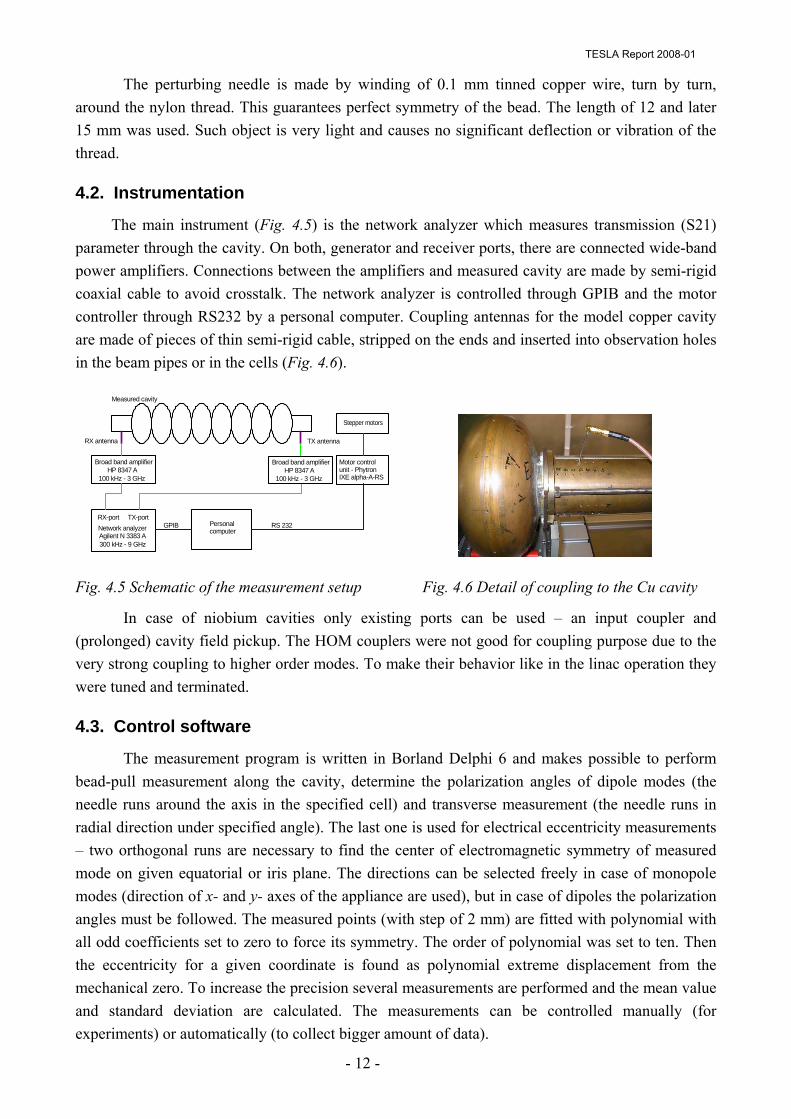
The main instrument (Fig. 4.5) is the network analyzer which measures transmission (S21) parameter through the cavity. On both, generator and receiver ports, there are connected wide-band power amplifiers. Connections between the amplifiers and measured cavity are made by semi-rigid coaxial cable to avoid crosstalk. The network analyzer is controlled through GPIB and the motor controller through RS232 by a personal computer. Coupling antennas for the model copper cavity are made of pieces of thin semi-rigid cable, stripped on the ends and inserted into observation holes in the beam pipes or in the cells (Fig. 4.6).

Stepper motors

Motor controlunit - PhytronIXE alpha-A-RS

TX antennaRX antenna

Measured cavity

Broad band amplifier

Network analyzerRX-port TX-port

Personalcomputer

GPIB RS 232

HP 8347 A100 kHz - 3 GHz

Broad band amplifierHP 8347 A

100 kHz - 3 GHz

Agilent N 3383 A300 kHz - 9 GHz

Fig. 4.5 Schematic of the measurement setup Fig. 4.6 Detail of coupling to the Cu cavity

In case of niobium cavities only existing ports can be used – an input coupler and (prolonged) cavity field pickup. The HOM couplers were not good for coupling purpose due to the very strong coupling to higher order modes. To make their behavior like in the linac operation they were tuned and terminated.

4.3. Control software

The measurement program is written in Borland Delphi 6 and makes possible to perform bead-pull measurement along the cavity, determine the polarization angles of dipole modes (the needle runs around the axis in the specified cell) and transverse measurement (the needle runs in radial direction under specified angle). The last one is used for electrical eccentricity measurements – two orthogonal runs are necessary to find the center of electromagnetic symmetry of measured mode on given equatorial or iris plane. The directions can be selected freely in case of monopole modes (direction of x- and y- axes of the appliance are used), but in case of dipoles the polarization angles must be followed. The measured points (with step of 2 mm) are fitted with polynomial with all odd coefficients set to zero to force its symmetry. The order of polynomial was set to ten. Then the eccentricity for a given coordinate is found as polynomial extreme displacement from the mechanical zero. To increase the precision several measurements are performed and the mean value and standard deviation are calculated. The measurements can be controlled manually (for experiments) or automatically (to collect bigger amount of data).


- 13 -

5. Calculation of electrical axis of the TM010-π mode

The goal of the cell alignment is to minimize the eccentricity of each cell. As the eccentricities cannot be set exactly to zero values, the electrical axis for the accelerating mode must be calculated and the cavity must be fixed in the cryomodule with certain tilt in order to pass the beam through the electrical axis. The tolerances for beam trajectory in respect to the electrical axis are 0.5 mm for offset and 0.5 mrad for tilt. We assume equal electric field distribution among cells what is a goal of cavity tuning. The electrical axis will be calculated as a straight line with minimal sum of quadratic deviations from measured electric centers of all cells. [6]

We will work in Cartesian coordinates with notation of xi and yi for x and y coordinate of the electrical center of i-th cell. We set the z-coordinate as variable. The deviation of the center of i-th cell from the electrical axis is given by:

iibai xzxxx −+=Δ )( (5.1)

iibai yzyyy −+=Δ )( (5.2)

Where xa and ya are zero order and xb and yb are first order parameters. The x and y coordinates are independent, they can be treated separately. In the following text we will find the xa and xb

parameters only. The equations for the y coordinate are identical. The equation (5.1) can be written in form (5.3) or (5.4):

⎟⎟⎟⎟⎟

⎠

⎞

⎜⎜⎜⎜⎜

⎝

⎛

Δ

ΔΔ

+

⎟⎟⎟⎟⎟

⎠

⎞

⎜⎜⎜⎜⎜

⎝

⎛

=⎟⎟⎠

⎞⎜⎜⎝

⎛⋅

⎟⎟⎟⎟⎟

⎠

⎞

⎜⎜⎜⎜⎜

⎝

⎛

9

2

1

9

2

1

9

2

1

1

11

x

xx

x

xx

xx

z

zz

b

a

MMMM (5.3)

XVXM x Δ+=⋅ (5.4)

The goal of optimization is:

∑=

=Δ9

1

2 min)(i

ix (5.5)

In order to satisfy equation (5.5) we evaluate the error vector ΔX from the (5.4), differentiate it over the variable z and set the result to zero. Then we evaluate the coefficient vector X (5.6) and identically the coefficient vector Y (5.7):

( ) xTT VMMMX ⋅⋅⋅=

−1 (5.6)

( ) yTT VMMMY ⋅⋅⋅=

−1 (5.7)


- 14 -

The position of electrical axis of measured will be later calculated as points where it passes equator planes of the first (5.8) and last cells (5.9).

⎟⎟⎠

⎞⎜⎜⎝

⎛=

a

a

yx

P1 (5.8)

⎟⎟⎠

⎞⎜⎜⎝

⎛⋅+⋅+

=ba

ba

ydyxdx

P88

9 (5.9)

where d is the distance between the cells (115.4 mm). Additionally the tilt of the electrical axis in respect to the z axis will be calculated in degrees (5.10).

( )22arctan180bb xx +⋅⎟

⎠⎞

⎜⎝⎛ °

=π

α (5.10)

6. Measurements of copper model cavity

These measurements were performed in order to evaluate the measurement method. The goal was to measure as many modes as possible and observe whether they have the same electrical eccentricity in same cells. This would be the case when the given cell is (or is not) shifted from the mechanical axis of the cavity, but has no deformations and is perfectly rotational symmetric. Otherwise different modes can have different centers due to their different field structure. The advantage of use of this cavity is flexibility to choose the location of coupling antennas (Fig. 4.6). This is very important for optimizing of coupling and polarizations separation of dipole HOMs. The dimensions of used metallic perturbing needle are 12 mm length and 0.3 mm diameter.

At first the bead-pull measurements for modes TM010, TM110 and TM011 were performed. This was necessary to explore the field pattern along the z-axis and determine cells with sufficient amount of stored energy for given modes, which is necessary to perform the measurement. For dipole modes also the polarization planes must be determined. Then by use of selected modes transverse measurements were done, the electrical centers of cells found and results were compared in polar coordinates. Unfortunately the reference rings of the copper cavity are not precisely soldered (the distance between their centers in the xy-plane is 0.5 mm) and therefore electromagnetic measurement results could be compared one with another (relative), but not with the mechanical measurement made on the machine with another fixation of the cavity.

6.1. TM010 passband

The TM010 modes were measured on equators (average of 10 measurements) and on iris (average of 5 measurements). The measurements on equators were made for all cells with sufficient amount of stored energy at given modes. Modes for iris measurements were selected as shown on Fig. 6.1 – 6.3. They have continuous Ez component on measured iris plane and not too different electric field intensities in adjacent cells.


- 15 -

Fig. 6.1 TM010-4π/9 suitable for irises 1 and 8 Fig. 6.2 TM010-2π/9 suitable for irises 2, 3, 6, 7

Fig. 6.3 TM010-π/9 suitable for irises 3 – 6

The results of 10 measurements per mode, cell and direction (0° and 90°) for equators and of 5 measurements per mode, cell and direction for irises were averaged, standard deviations were calculated and converted to polar coordinates (Fig. 6.4 - 6.8), Finally, the average values of all measured modes for each equator and iris were calculated and compared one with another (Fig. 6.9, 6.10).

0

0.2

0.4

0.6

0.8

1

1.2

1 2 3 4 5 6 7 8 9Cell number

Ecce

ntric

ity -

radi

us [m

m]

TM010 pi/9

TM010 2pi/9

TM010 3pi/9

TM010 4pi/9

TM010 5pi/9

TM010 6pi/9

TM010 7pi/9

TM010 8pi/9

TM010 pi

-200

-180

-160

-140

-120

-100

-80

-60

-40

-20

0

1 2 3 4 5 6 7 8 9

Cell number

Ecce

ntric

ity -

angl

e [°

]

TM010 pi/9

TM010 2pi/9

TM010 3pi/9

TM010 4pi/9

TM010 5pi/9

TM010 6pi/9

TM010 7pi/9

TM010 8pi/9

TM010 pi

Fig. 6.4 Radius of eccentricity, equators Fig. 6.5 Angle of eccentricity, equators


- 16 -

0.000

0.020

0.040

0.060

0.080

0.100

0.120

0.140

1 2 3 4 5 6 7 8 9Cell number

Sta

ndar

d de

viat

ion

of ra

dial

ecc

entri

city

[mm

]

TM010 pi/9

TM010 2pi/9

TM010 3pi/9

TM010 4pi/9

TM010 5pi/9

TM010 6pi/9

TM010 7pi/9

TM010 8pi/9

TM010 pi

Fig. 6.6 Standard deviations of radial eccentricity, equators

0

0.2

0.4

0.6

0.8

1

1.2

1 2 3 4 5 6 7 8

Iris number

Ecce

ntric

ity -

radi

us [m

m]

TM010 pi/9

TM010 2pi/9

TM010 4pi/9

-180

-160

-140

-120

-100

-80

-60

-40

-20

0

1 2 3 4 5 6 7 8Iris number

Ecce

ntric

ity -

angl

e [°

]

TM010 pi/9

TM010 2pi/9

TM010 4pi/9

Fig. 6.7 Radius of eccentricity, irises Fig. 6.8 Angle of eccentricity, irises

0.00

0.20

0.40

0.60

0.80

1.00

1.20

1E 1I 2E 2I 3E 3I 4E 4I 5E 5I 6E 6I 7E 7I 8E 8I 9E

Equator(E) and iris (I) number

Ecce

ntric

ity -

radi

us [m

m]

-180

-160

-140

-120

-100

-80

-60

-40

-20

0

1E 1I 2E 2I 3E 3I 4E 4I 5E 5I 6E 6I 7E 7I 8E 8I 9E

Equator(E) and iris (I) number

Ecc

entri

city

- an

gle

[°]

Fig. 6.9 Comparison of eccentricity Fig. 6.10 Comparison of eccentricity of equators and irises (radius) of equators and irises (angle)

TM010 passband - conclusion:

• The maximum measured standard deviation of radial eccentricity was 0.12 mm, which satisfies expected error (0.1 mm in rectangular or 0.14 mm in polar coordinates).


- 17 -

• The eccentricity differences for various modes in the same cells are lower than the corresponding standard deviations, so assuming the available precision we can say that the eccentricities of different modes in the same cells are equal. It means that the rotation symmetry of cells, although the center of the cavity is displaced more then 1 mm from the mechanical axis, is not significantly perturbed.

• The eccentricities of irises follow the eccentricities of equators. It means, that in case of high precision cells (without significant deformations) and less demanding tasks fast measurements on irises can be used instead of time consuming measurements on equators.

6.2. TM110 passband

The modes of this passband are easily measurable on equatorial planes of cells due to sharp electric field minima on the axis. Unlike the monopole modes, the coordinate system for this measurement cannot be freely chosen but is determined by polarization angles which must be measured before. The equators of cells with enough stored energy for given modes were measured and the eccentricities were recalculated into polar coordinates. The results were compared with the average of TM010 eccentricities (red bars).

0

0.2

0.4

0.6

0.8

1

1.2

1.4

1 2 3 4 5 6 7 8 9Cell number

Ecce

ntric

ity -

radi

us [m

m]

TM110 pi/9

TM110 2pi/9

TM110 3pi/9

TM110 4pi/9

TM110 5pi/9

TM110 6pi/9

TM110 7pi/9

TM110 8pi/9

TM110 pi

TM010 average

-200

-180

-160

-140

-120

-100

-80

-60

-40

-20

0

1 2 3 4 5 6 7 8 9

Cell number

Ecce

ntric

ity -

angl

e [°

]

TM110 pi/9

TM110 2pi/9

TM110 3pi/9

TM110 4pi/9

TM110 5pi/9

TM110 6pi/9

TM110 7pi/9

TM110 8pi/9

TM110 pi

TM010 average

Fig. 6.11 Radius of eccentricity Fig. 6.12 Angle of eccentricity

0.000

0.020

0.040

0.060

0.080

0.100

0.120

0.140

0.160

1 2 3 4 5 6 7 8 9Cell number

Stan

dard

dev

iatio

n of

radi

al e

ccen

trici

ty [m

m]

TM110 pi/9

TM110 2pi/9

TM110 3pi/9

TM110 4pi/9

TM110 5pi/9

TM110 6pi/9

TM110 7pi/9

TM110 8pi/9

TM110 pi

Fig. 6.13 Standard deviations of radial eccentricity


- 18 -

TM110 passband - conclusion:

• The expected precision is satisfied.

• The differences between modes (also in comparison with the average of all measured TM010

modes) are bigger as in case of TM010 modes. The TM110 modes are more sensitive to deformations of cells due to their different field pattern. Maximum measured difference of radius of eccentricity is approximately 0.2 mm.

6.3. TM011 passband

TM011 is the second monopole passband. The coordinate system can be chosen arbitrarily. With the existing measurement setup only irises could be measured. The used modes (5π/9 up to π) have sufficiently strong local electric field maxima on measured irises. The results are on Fig. 6.14 - 6.16. They are compared also with the average eccentricity of TM010 modes on irises (red bars).

0

0.2

0.4

0.6

0.8

1

1.2

1.4

1 2 3 4 5 6 7 8Iris number

Ecce

ntric

ity -

radi

us [m

m]

TM011 pi

TM011 8pi/9

TM011 7pi/9

TM011 6pi/9

TM011 5pi/9

TM010 average

-200

-180

-160

-140

-120

-100

-80

-60

-40

-20

0

1 2 3 4 5 6 7 8Iris number

Ecce

ntric

ity -

angl

e [°

]

TM011 pi

TM011 8pi/9

TM011 7pi/9

TM011 6pi/9

TM011 5pi/9

TM010 average

Fig. 6.14 Radius of eccentricity, irises Fig.6.15 Angle of eccentricity, irises

0.000

0.010

0.020

0.030

0.040

0.050

0.060

0.070

0.080

0.090

1 2 3 4 5 6 7 8Iris number

Ecce

ntric

ity -

radi

us [m

m]

TM011 pi

TM011 8pi/9

TM011 7pi/9

TM011 6pi/9

TM011 5pi/9

Fig. 6.16 Standard deviations of radial eccentricity


- 19 -

TM011 passband- conclusion:

• The expected precision is satisfied.

• Differences between many modes lie below 0.1 mm, but also some differences about 0.2 mm are present. This can be caused not only by cell deformations, but also by imperfection of beam pipes, because they are close to the cut-off and some modes store significant amount of energy there. The coupling between cells is also very strong, so one cell or a beam pipe could significantly influence the whole structure. On the other side the beam pipes are long enough to suppress the influence of open boundaries. This was tested by comparison of field eccentricity on the iris nr. 1 with and without large perturbing object (nut M16) placed at the end of the beam pipe. No difference was detected.

7. Measurements of niobium cavity

The experiments with copper cavity are very comfortable and have great scientific value. The niobium cavities have a lot of limitation in the measurements. All ports of the cavity (input coupler, HOM couplers, and field pickup) are fixed and there is no other way to couple RF power to and from the cavity. The coupling to the TM010-π/9 mode was so weak that this measurement was not possible. As this mode is necessary to measure irises nr. 3 – 6, the measurement on irises was omitted. Also the dipole modes could not be measured because the port locations could not be matched to their polarizations planes. The band TM011 was measured, but the field in cells 1 and 2 was strongly influenced by the following quadrupole passband, so these results have little value.

The cavity used for these measurements was received in coarse pre-tuned state (after electropolishing). The first set of measurements was done in this state and a metallic needle with diameter 0.3 mm and length 12 mm was used as perturbing bead. The second set of measurements was performed after the precise (according to the mechanical measurement) tuning. The results with the 12 mm needle were too noisy (probably due to lower temperature stability than in the previous case), so the needle was prolonged to 15 mm. The HOM couplers were tuned and terminated before the measurements to behave in the same way as in operation. As explained above, only TM010 passband on equators gave reasonable results. Comparison with mechanically measured eccentricities (red bars on the charts) was also done and the electric and geometrical axis positions for the accelerating mode were calculated and compared. Finally, the electrical axis for the accelerating mode and geometrical axis were calculated. The position of the electrical (Tab. 7.1, Fig. 7.5 left) and geometrical (Tab. 7.2, Fig. 7.5 left) axis was evaluated in respect to the cavity axis (in the coordinate system of the measurement equipment) and in respect to the geometrical axis (Tab. 7.3, Fig. 7.5 right) - or in respect to the beam, if the geometrical axis, as done until now, is aligned with the beam trajectory).


- 20 -

0.00

0.10

0.20

0.30

0.40

0.50

0.60

0.70

1 2 3 4 5 6 7 8 9Cell number

Ecce

ntric

ity -

radi

us [m

m]

TM010 pi/9

TM010 2pi/9

TM010 3pi/9

TM010 4pi/9

TM010 5pi/9

TM010 6pi/9

TM010 7pi/9

TM010 8pi/9

TM010 pi

Mechanic

0

0.1

0.2

0.3

0.4

0.5

0.6

1 2 3 4 5 6 7 8 9

Cell number

Ecce

ntric

ity -

radi

us [m

m]

TM010 pi/9

TM010 2pi/9

TM010 3pi/9

TM010 4pi/9

TM010 5pi/9

TM010 6pi/9

TM010 7pi/9

TM010 8pi/9

TM010 pi

Mechanic

Fig. 7.1 Radius of eccentricity, coarse pre-tuned Fig. 7.2 Radius of eccentricity, tuned

-50

0

50

100

150

200

1 2 3 4 5 6 7 8 9Cell number

Ecce

ntric

ity -

angl

e [°

]

TM010 pi/9

TM010 2pi/9

TM010 3pi/9

TM010 4pi/9

TM010 5pi/9

TM010 6pi/9

TM010 7pi/9

TM010 8pi/9

TM010 pi

Mechanic

-200

-150

-100

-50

0

50

100

150

200

1 2 3 4 5 6 7 8 9Cell number

Ecce

ntric

ity -

angl

e [°]

TM010 pi/9

TM010 2pi/9

TM010 3pi/9

TM010 4pi/9

TM010 5pi/9

TM010 6pi/9

TM010 7pi/9

TM010 8pi/9

TM010 pi

Mechanic

Fig. 7.3 Angle of eccentricity, coarse pre-tuned Fig. 7.4 Angle of eccentricity, tuned

Tab.7.1 Position of electrical axis of accelerating mode

Cavity state Equator plane 1 crossing [mm] Equator plane 9 crossing [mm] Tilt [μrad]

Pre-tuned (-0.325, 0.208) (-0.02, 0.12) 344 Final tuned (-0.156, 0.116) (0.177, 0.033) 371

Tab. 7.2 Position of geometrical axis

Cavity state Equator plane 1 crossing [mm] Equator plane 9 crossing [mm] Tilt [μrad] Pre-tuned (0.06, 0.03) (0.201, 0.036) 153

Final tuned (0.017, 0.008) (0.215, -0.005) 216

Tab. 7.3 Position of electrical axis in respect to the geometrical axis

Cavity state Equator plane 1 crossing [mm] Equator plane 9 crossing [mm] Tilt [μrad] Pre-tuned (-0.265, 0.238) (0.181, 0.155) 491

Final tuned (-0.139, 0.125) (0.392, 0.028) 585


- 21 -

Fig. 7.5 Position of electrical and geometrical axes in respect to the cavity axis (left) and position of electrical axis in respect to the geometrical axis (right)

TM010 passband – conclusion:

• Standard deviations are higher than in case of the copper cavity, but the precision requirement is still satisfied. The signal noise results from the fixed antenna location (optimization of coupling was not possible) and also from two times lower unloaded quality factor of the niobium cavity in comparison to the copper one.

• Differences between some modes are significant; it means that the cell walls are slightly deformed. Please note that although the mechanical eccentricity of the cell nr. 4 was significantly reduced – by 0.3 mm, the electrical eccentricity only by something above 0.1 mm. The mechanical eccentricities of cells nr. 5 and 6 were also successfully lowered, but the electrical centers went to another direction. The tilt of the electrical axis of the accelerating mode was increased by the final tuning from 491 μrad to 585 μrad. This is the evidence of precision limit of the mechanical method.

• Maximum difference between the electrical eccentricity of the accelerating π-mode and the mechanical eccentricity measured in classical way (cell 5, final tuned cavity) is below the accepted tolerance of 0.4 mm. Position of the electrical axis in respect to the geometrical one lies also inside the tolerance band, which is 0.5 mm for offset and 0.5 mrad for tilt.


- 22 -

8. Conclusion • The possibility of using of small perturbation for cavity eccentricity measurement was

theoretically analyzed and consequently the measurement equipment was designed, built and control software was written.

• In the case of copper cavity the random error of all measurements is below the expected limit (0.1 mm in rectangular or 0.14 mm in polar coordinates). Under good conditions (sufficiently strong coupling of antennas and stable temperature) the standard deviation in many cases is even below 50 μm. In the niobium cavity it is - due to suboptimal coupling - worse , but still sufficiently precise.

• In the copper cavity a complete set of TM010, TM110 and TM011 modes was measured. Though the center of the cavity is displaced by more than 1 mm from the cavity axis, the cells keep the rotation symmetry and the spread of their electrical centers for different TM010

modes is below the measurement noise level. For higher order modes the spread of electrical eccentricity is greater – up to 0.2 mm.

• Due to the limitations of coupling possibilities to the niobium cavity only the TM010 passband measurement gave reasonable results. The spread of electrical centers of various modes in the same cells is greater than in the case of copper cavity. This indicates small deformation of cavity wall.

• The performed tuning with goal of minimization of geometrical eccentricity slightly increased the electrical eccentricity of some cells and the tilt of electrical axis. This indicates that the mechanical measurement method matches the electrical eccentricity only with a precision of few tenths of mm.

• The difference between the mechanical and electrical eccentricity lies below the accepted error of 0.4 mm and the misalignment between electrical and geometrical axis below tolerated 0.5 mm and 0.5 mrad. The measurements of another two niobium cavities gave similar results. In case no increase of precision will be required the mechanical measurement is sufficient. To increase the precision of cavity measurement and/or tuning the small perturbation measurement would be necessary.


- 23 -

References

[1] Martin Nagl, DESY, group MIN: Consultations and hand written notes

[2] O. S. Milovanov, N. P. Sobenin: “Ultra High Frequency Engineering”, Atomizdat, Moscow, Russia, 1980

[3] Robert E. Collin: “Foundation for Microwave Engineering”, McGraw-Hill, 2-nd edition, USA, 1992, ISBN: 0-07-112569-8

[4] L.C. Maier Jr, J.C. Slater: “Field Strength Measurements in Resonant Cavities”, Research laboratory of Electronics, MIT, Cambridge, Massachusetts, USA, 1951

[5] P. M. Lapostolle, A. L. Septier: “Linear Accelerators”, North Holland Pub. Co., Amsterdam, Holland, 1970

[6] Martin Dohlus, DESY, group MPY: Consultations

Acknowledgements

I would like to sincerely thank my colleagues for great help with this work: • Jacek Sekutowicz, Martin Nagl and Martin Dohlus for theoretical support • Guennadi Kreps and Wolf-Dietrich Möller for measurement advices and many useful proposals • Daniel Klinke and Hans-Bernhard Peters for mechanical design


electrical axes of tesla-type cavities - desy - flash ... · electrical axes of tesla-type cavities...

Documents