electrical power cables – part 2 cable rating … - lec4 - cables... · the calculation of cable...
TRANSCRIPT
ELEC9712: Power Cables – Part 2 p. 1/32
ELEC9712 High Voltage Systems
Electrical Power Cables – Part 2 Cable Rating Calculations
The calculation of cable ratings is a very complex determination because of the large number of interacting characteristics and parameters involved in the establishment of a heat balance (for steady state ratings) or general heat dissipation/heat generation equation (for transient ratings). The cable heat dissipation is achieved by means of thermal conduction to the cable surface (an inefficient heat transfer process compared to convection and radiation transfer). From the cable surface heat is then dissipated by a variety of means, depending on the cable installation, the ambient conditions and the general configuration. The cable thermal properties and also the thermal characteristics of the environment of the cable installation are thus very important in the rating calculations. 1. Cable installation methods Cables are installed in a very large variety of environments, including the following examples:
ELEC9712: Power Cables – Part 2 p. 2/32
Direct burial in the ground with no special backfill material
Burial in a trench packed with thermally enhanced dissipation material
Installation in ducts or pipes buried in the ground
Installation in a duct or pipe situated in open air
Installation in large diameter tunnels
Installation directly in open air situations
Undersea: open or buried
In troughs with circulating water In addition to the usual case of internal heat generation in a single cable (self-heating), it will generally be the case that cables will be installed in closely-coupled three phase groups or even double circuit arrangements of six cables. The result of this close interaction will be that mutual heat generation between cables must also be taken into consideration when determining the heat generation level. In all of these cases the thermal properties, including the thermal resistances, of the material surrounding the cable must be known in detail so that the heat dissipation rates from the cable surface to the infinite heat sink at ambient temperature can be determined. It is also necessary to determine such details, particularly the internal thermal resistances, for the cable and its component parts and materials.
ELEC9712: Power Cables – Part 2 p. 3/32
In particular, the following are the important material characteristics required:
thermal resistivity of insulation (g: oC/W or thermal Ω.m)
specific heat of insulation and of the metal (c: J/kg/C)
mass density of the insulation and the metal (δ : kg/m3) The thermal resistivity (g) of the various materials is of major importance in determining the thermal resistance of various parts of the thermal circuit used for steady state rating calculations. The thermal diffusivity of the insulation, defined as:
1. .g c
αδ
= [m2/s]
is also an important parameter for transient rating calculations of buried cables. In this case the heat storage characteristics are important. Typical values of the above quantities for some relevant materials are shown in the accompanying table. The thermal diffusivity of different soil materials does not vary very much, being generally in the range of about 1.0 ± 0.8 m2/sec. An average value of about 0.6 is often used. A value of soil thermal resistivity of 1.2 thermal Ω.m is often used. Typically insulation materials will have thermal resistivities of about 5-6 thermal Ω.m.
ELEC9712: Power Cables – Part 2 p. 4/32
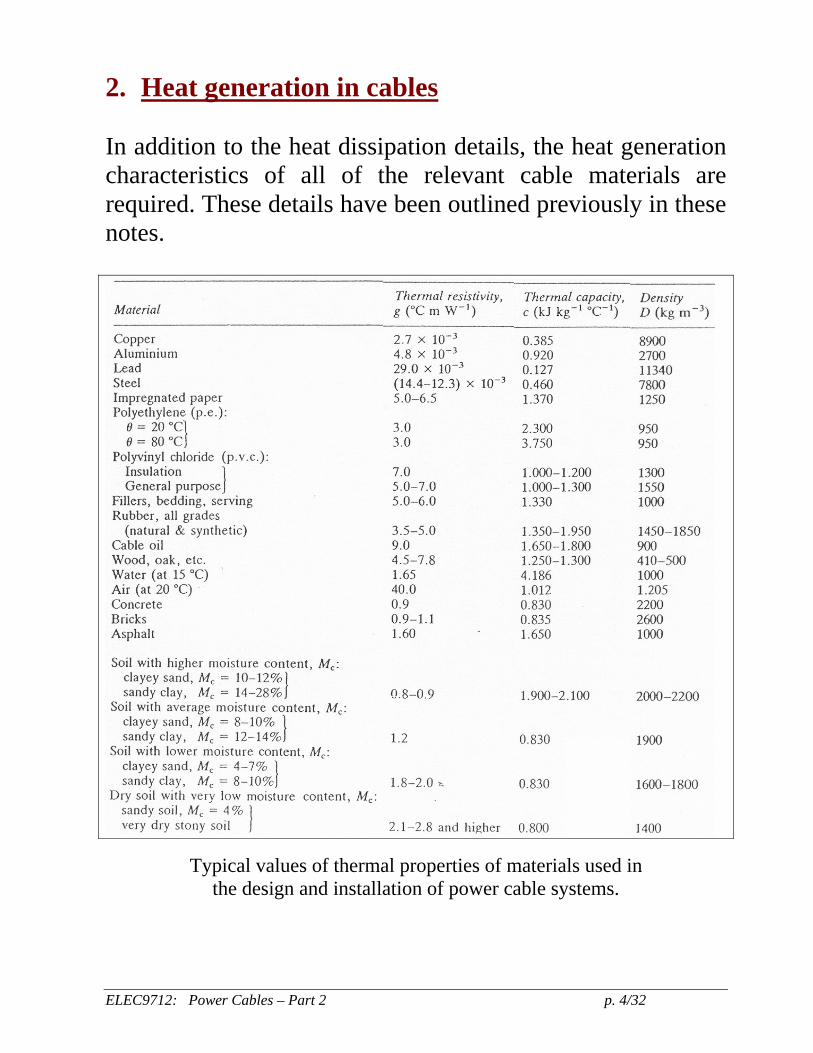
2. Heat generation in cables In addition to the heat dissipation details, the heat generation characteristics of all of the relevant cable materials are required. These details have been outlined previously in these notes.
Typical values of thermal properties of materials used in the design and installation of power cable systems.
ELEC9712: Power Cables – Part 2 p. 5/32
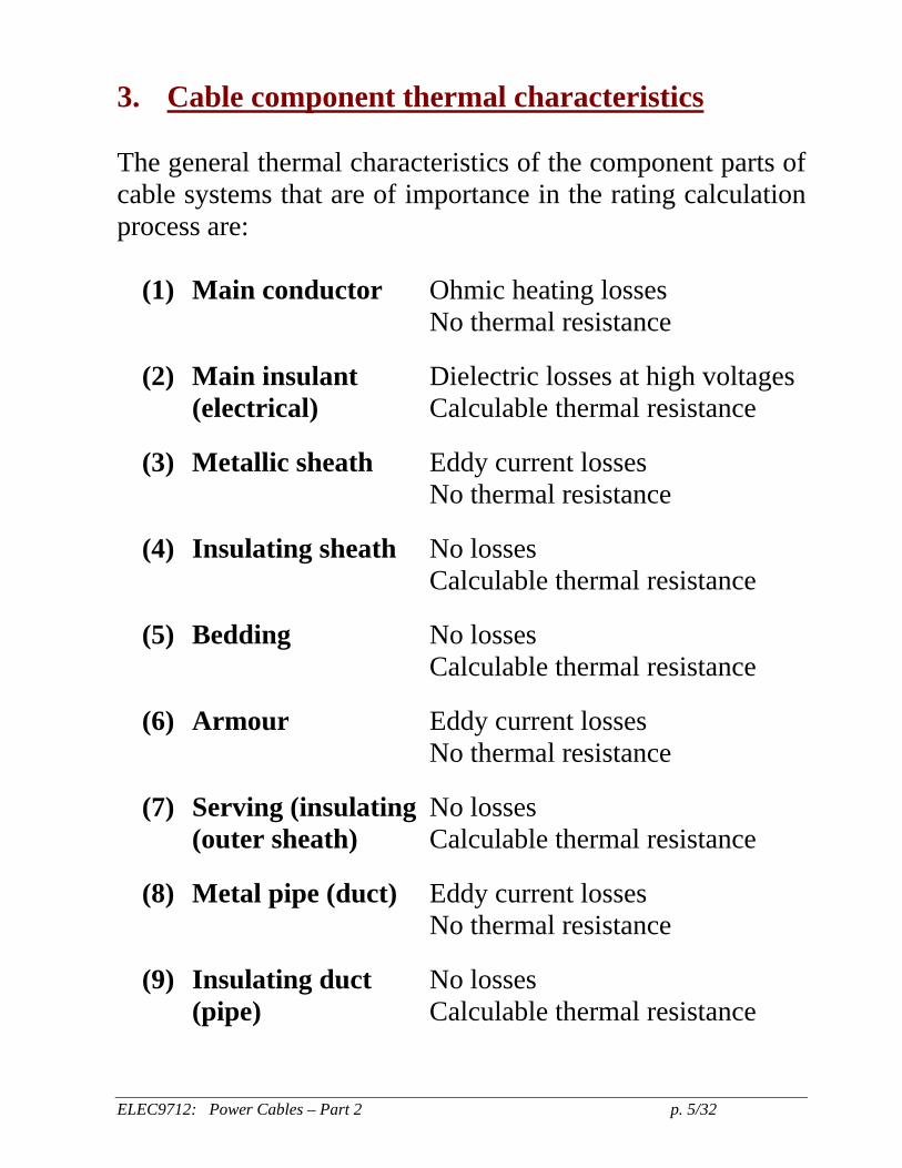
3. Cable component thermal characteristics The general thermal characteristics of the component parts of cable systems that are of importance in the rating calculation process are:
(1) Main conductor Ohmic heating losses No thermal resistance (2) Main insulant Dielectric losses at high voltages (electrical) Calculable thermal resistance (3) Metallic sheath Eddy current losses No thermal resistance (4) Insulating sheath No losses Calculable thermal resistance (5) Bedding No losses Calculable thermal resistance (6) Armour Eddy current losses No thermal resistance (7) Serving (insulating No losses (outer sheath) Calculable thermal resistance (8) Metal pipe (duct) Eddy current losses No thermal resistance (9) Insulating duct No losses (pipe) Calculable thermal resistance
ELEC9712: Power Cables – Part 2 p. 6/32
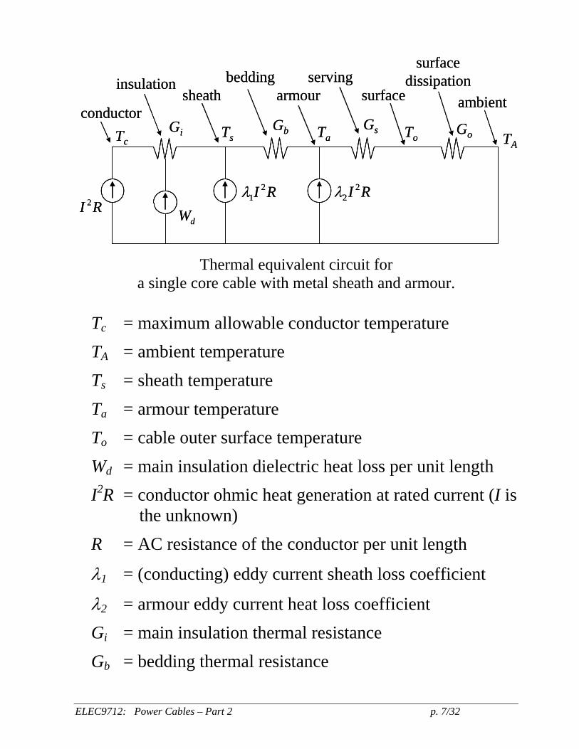
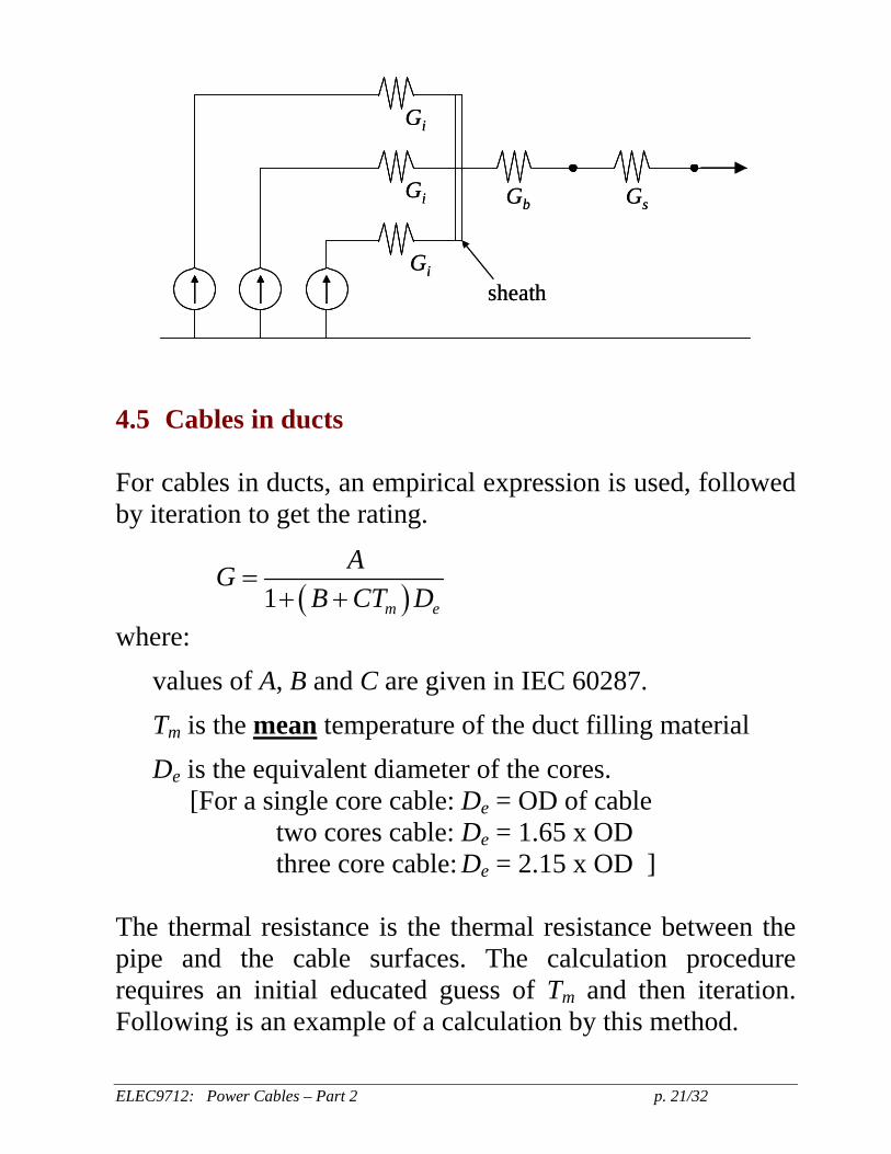
In addition to the thermal characteristics of the cable components, the thermal characteristics of the cable installation environment are also required: these include, for example, the ground (soil) thermal resistance, the air thermal resistance and the associated heat capacities and diffusivities etc. If the cable is in open air, the radiative and convective dissipation properties are also needed. 3.1 Equivalent Steady State Thermal Circuit The general thermal equivalent circuit used for steady state rating calculation is shown below. It is an electrical-thermal analogy using the heat generation as the equivalent current sources, the thermal resistances for electrical resistances and the temperature as the voltage potential analogue. From the equivalent circuit it can be seen that it is necessary to calculate accurately the thermal resistances and the heat generation losses and to be able to specify the fixed temperatures at the conductor and at the ambient condition (the ground surface, for example). The unknown is the current level (the thermal rating) which will be determined by the heat balance at steady state operation.
ELEC9712: Power Cables – Part 2 p. 7/32
Gi
ambient
2I R
conductorsheath
dW
21I Rλ 2
2I Rλ
TA Tc
Gb Gs Go
insulation
Ts
beddingarmour
Ta
serving
To
surface
surfacedissipation
Gi
ambient
2I R
conductorsheath
dW
21I Rλ 2
2I Rλ
TA Tc
Gb Gs Go
insulation
Ts
beddingarmour
Ta
serving
To
surface
surfacedissipation
Thermal equivalent circuit for a single core cable with metal sheath and armour.
Tc = maximum allowable conductor temperature
TA = ambient temperature
Ts = sheath temperature
Ta = armour temperature
To = cable outer surface temperature
Wd = main insulation dielectric heat loss per unit length
I2R = conductor ohmic heat generation at rated current (I is the unknown)
R = AC resistance of the conductor per unit length
λ1 = (conducting) eddy current sheath loss coefficient
λ2 = armour eddy current heat loss coefficient
Gi = main insulation thermal resistance
Gb = bedding thermal resistance
ELEC9712: Power Cables – Part 2 p. 8/32
Gs = serving or insulating sheath thermal resistance
Go = effective thermal resistance between the cable surface and the ambient
Go will depend on the nature of the cable installation and may ultimately be the most difficult quantity to evaluate accurately, particularly when the cable surface is open to air or fluid environments. Note that the (distributed) dielectric heat generation Wd is normally included at the mid-point of the insulation resistance, so that Wd passes through only half of the thermal resistance. It can be shown mathematically that the temperature rise of insulation due to dielectric heating is:
12 d iT W GΔ = ×
Thus it is necessary to place the dielectric heat input at the midpoint of Gi in the equivalent circuit. 3.1.1 Specified Conductor Temperature The maximum conductor temperature to be used in the calculation will be that specified by the manufacturer as the maximum permissible steady state temperature of the insulation material that is in contact with the main insulation. Some typical upper limits of temperature are shown over.
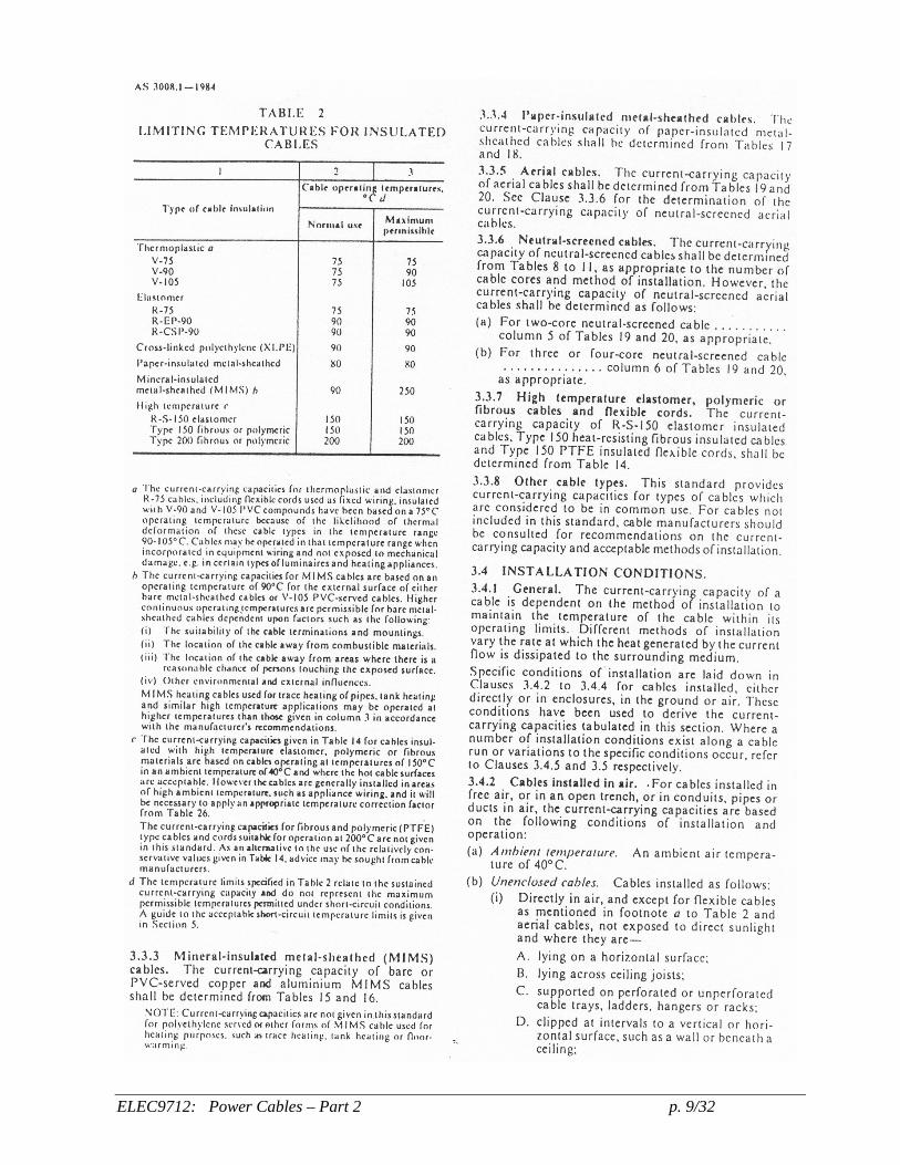
ELEC9712: Power Cables – Part 2 p. 9/32
ELEC9712: Power Cables – Part 2 p. 10/32
ELEC9712: Power Cables – Part 2 p. 11/32
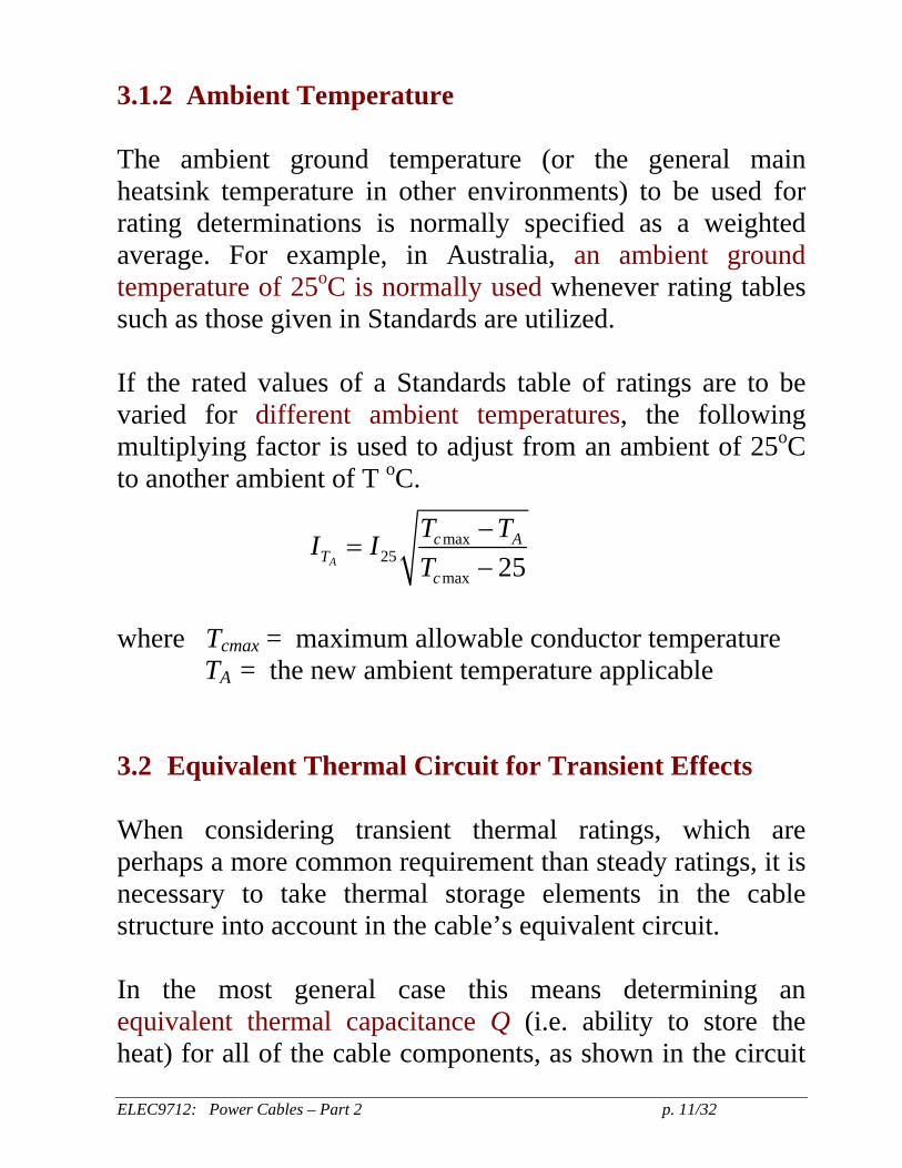
3.1.2 Ambient Temperature The ambient ground temperature (or the general main heatsink temperature in other environments) to be used for rating determinations is normally specified as a weighted average. For example, in Australia, an ambient ground temperature of 25oC is normally used whenever rating tables such as those given in Standards are utilized. If the rated values of a Standards table of ratings are to be varied for different ambient temperatures, the following multiplying factor is used to adjust from an ambient of 25oC to another ambient of T oC.
max25
max 25A
c AT
c
T TI IT
−=
−
where Tcmax = maximum allowable conductor temperature TA = the new ambient temperature applicable 3.2 Equivalent Thermal Circuit for Transient Effects When considering transient thermal ratings, which are perhaps a more common requirement than steady ratings, it is necessary to take thermal storage elements in the cable structure into account in the cable’s equivalent circuit. In the most general case this means determining an equivalent thermal capacitance Q (i.e. ability to store the heat) for all of the cable components, as shown in the circuit
ELEC9712: Power Cables – Part 2 p. 12/32
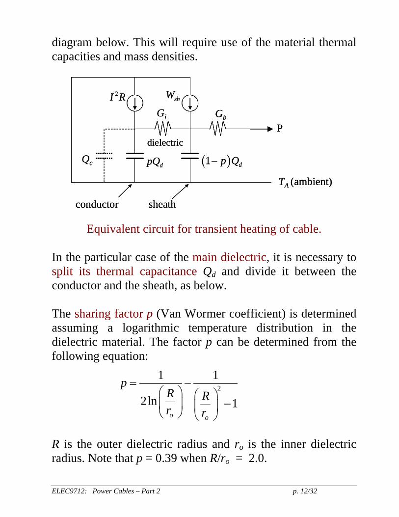
diagram below. This will require use of the material thermal capacities and mass densities.
( )1 dp Q−
Gi Gb
Qc
TA (ambient)
dpQ
Pdielectric
2I R shW
conductor sheath
( )1 dp Q−
Gi Gb
Qc
TA (ambient)
dpQ
Pdielectric
2I R shW
conductor sheath
Equivalent circuit for transient heating of cable. In the particular case of the main dielectric, it is necessary to split its thermal capacitance Qd and divide it between the conductor and the sheath, as below. The sharing factor p (Van Wormer coefficient) is determined assuming a logarithmic temperature distribution in the dielectric material. The factor p can be determined from the following equation:
21 1
2ln 1o o
pR Rr r
= −⎛ ⎞ ⎛ ⎞
−⎜ ⎟ ⎜ ⎟⎝ ⎠ ⎝ ⎠
R is the outer dielectric radius and ro is the inner dielectric radius. Note that p = 0.39 when R/ro = 2.0.
ELEC9712: Power Cables – Part 2 p. 13/32
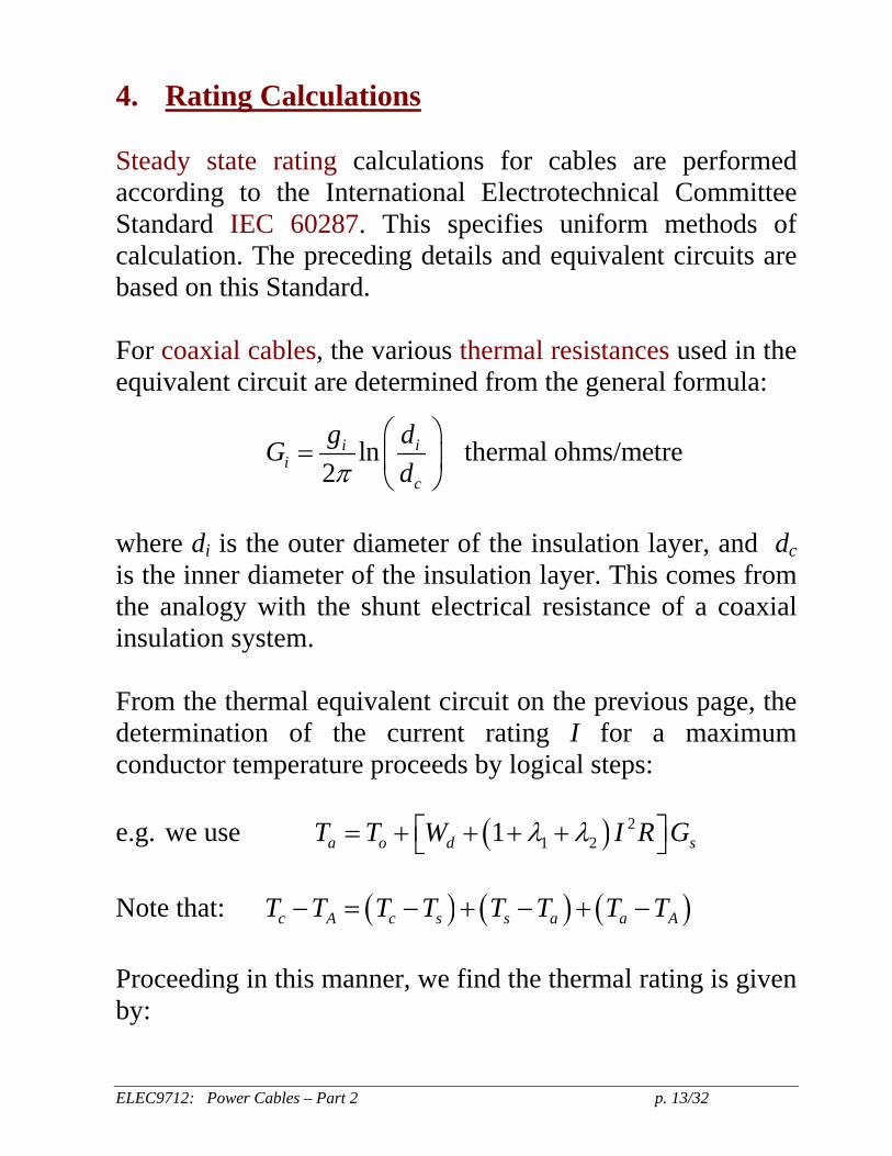
4. Rating Calculations Steady state rating calculations for cables are performed according to the International Electrotechnical Committee Standard IEC 60287. This specifies uniform methods of calculation. The preceding details and equivalent circuits are based on this Standard. For coaxial cables, the various thermal resistances used in the equivalent circuit are determined from the general formula:
ln thermal ohms/metre2
i ii
c
g dGdπ
⎛ ⎞= ⎜ ⎟
⎝ ⎠
where di is the outer diameter of the insulation layer, and dc is the inner diameter of the insulation layer. This comes from the analogy with the shunt electrical resistance of a coaxial insulation system. From the thermal equivalent circuit on the previous page, the determination of the current rating I for a maximum conductor temperature proceeds by logical steps: e.g. we use ( ) 2
1 21a o d sT T W I R Gλ λ⎡ ⎤= + + + +⎣ ⎦ Note that: ( ) ( ) ( )c A c s s a a AT T T T T T T T− = − + − + − Proceeding in this manner, we find the thermal rating is given by:
ELEC9712: Power Cables – Part 2 p. 14/32
[ ]
( ) ( )( )
1/ 2
1 1 2
12
1 1
c A d i b s o
i b s o
T T W G G G GI
RG R G R G Gλ λ λ
⎡ ⎤⎛ ⎞− − + + +⎜ ⎟⎢ ⎥⎝ ⎠⎢ ⎥=+ + + + + +⎢ ⎥
⎢ ⎥⎣ ⎦
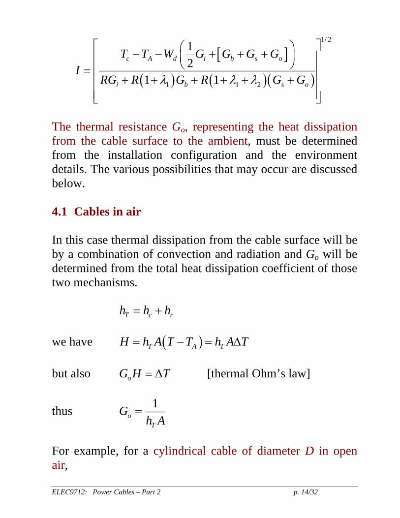
The thermal resistance Go, representing the heat dissipation from the cable surface to the ambient, must be determined from the installation configuration and the environment details. The various possibilities that may occur are discussed below. 4.1 Cables in air In this case thermal dissipation from the cable surface will be by a combination of convection and radiation and Go will be determined from the total heat dissipation coefficient of those two mechanisms. T c rh h h= + we have ( )T A TH h A T T h A T= − = Δ but also oG H T= Δ [thermal Ohm’s law]
thus 1o
T
Gh A
=
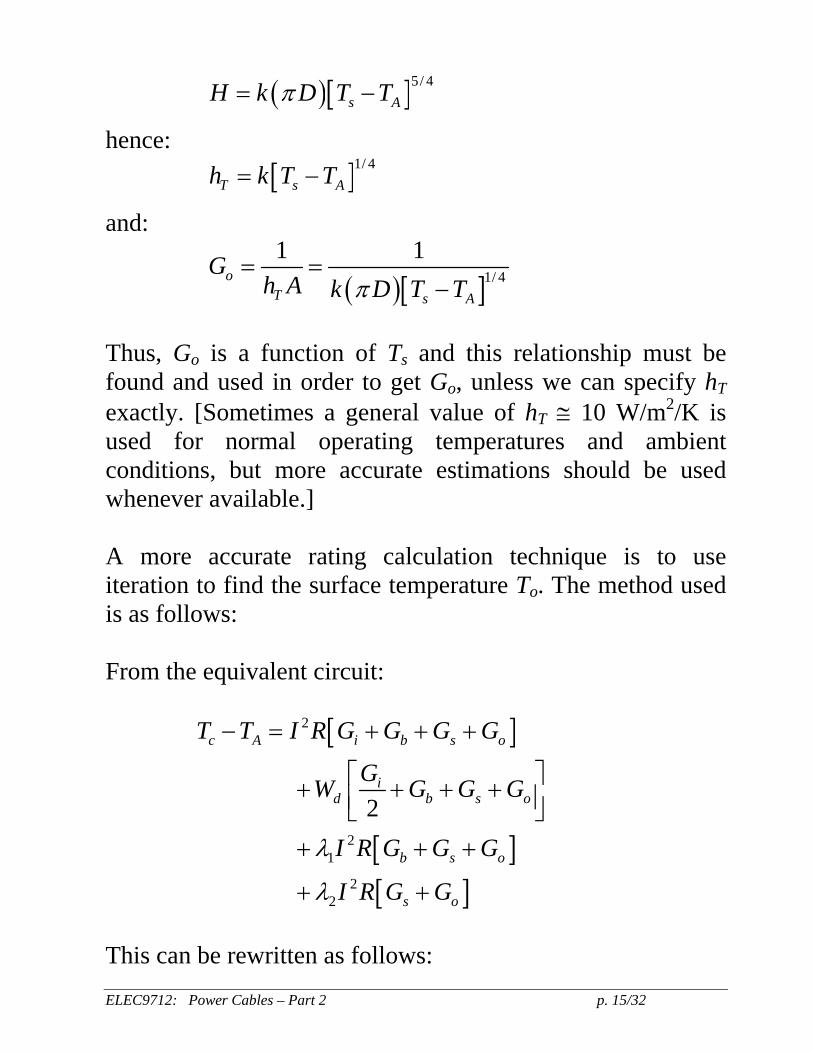
For example, for a cylindrical cable of diameter D in open air,
ELEC9712: Power Cables – Part 2 p. 15/32
( )[ ]5/ 4s AH k D T Tπ= −
hence: [ ]1/ 4
T s Ah k T T= −
and:
( )[ ]1/ 4
1 1o
T s A
Gh A k D T Tπ
= =−
Thus, Go is a function of Ts and this relationship must be found and used in order to get Go, unless we can specify hT exactly. [Sometimes a general value of hT ≅ 10 W/m2/K is used for normal operating temperatures and ambient conditions, but more accurate estimations should be used whenever available.] A more accurate rating calculation technique is to use iteration to find the surface temperature To. The method used is as follows: From the equivalent circuit:
[ ]
[ ][ ]
2
21
22
2
c A i b s o
id b s o
b s o
s o
T T I R G G G G
GW G G G
I R G G G
I R G G
λ
λ
− = + + +
⎡ ⎤+ + + +⎢ ⎥⎣ ⎦+ + +
+ +
This can be rewritten as follows:
ELEC9712: Power Cables – Part 2 p. 16/32
[ ]
[ ][ ]
[ ]
2
21
22
2
c A i b s
id b s
b s
s
o A
T T I R G G G
GW G G
I R G G
I R G
T T
λ
λ
− = + +
⎡ ⎤+ + +⎢ ⎥⎣ ⎦+ +
+
+ −
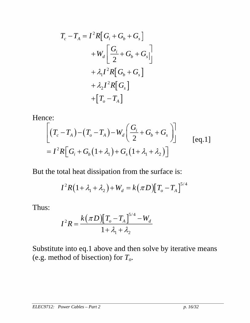
Hence:
( ) ( )
( ) ( )21 1 2
2
1 1
ic A o A d b s
i b s
GT T T T W G G
I R G G Gλ λ λ
⎡ ⎤⎛ ⎞− − − − + +⎜ ⎟⎢ ⎥⎝ ⎠⎣ ⎦⎡ ⎤= + + + + +⎣ ⎦
[eq.1]
But the total heat dissipation from the surface is:
( ) ( )[ ]5/ 421 21 d o AI R W k D T Tλ λ π+ + + = −
Thus:
( )[ ]5/ 42
1 21o A dk D T T W
I Rπ
λ λ− −
=+ +
Substitute into eq.1 above and then solve by iterative means (e.g. method of bisection) for To.
ELEC9712: Power Cables – Part 2 p. 17/32
4.2 Cables in ducts, pipes etc. In this case Go is the sum of the various thermal resistances in series:
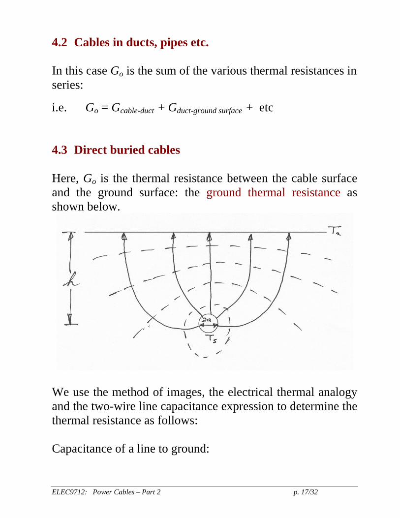
i.e. Go = Gcable-duct + Gduct-ground surface + etc 4.3 Direct buried cables Here, Go is the thermal resistance between the cable surface and the ground surface: the ground thermal resistance as shown below.
We use the method of images, the electrical thermal analogy and the two-wire line capacitance expression to determine the thermal resistance as follows: Capacitance of a line to ground:
ELEC9712: Power Cables – Part 2 p. 18/32
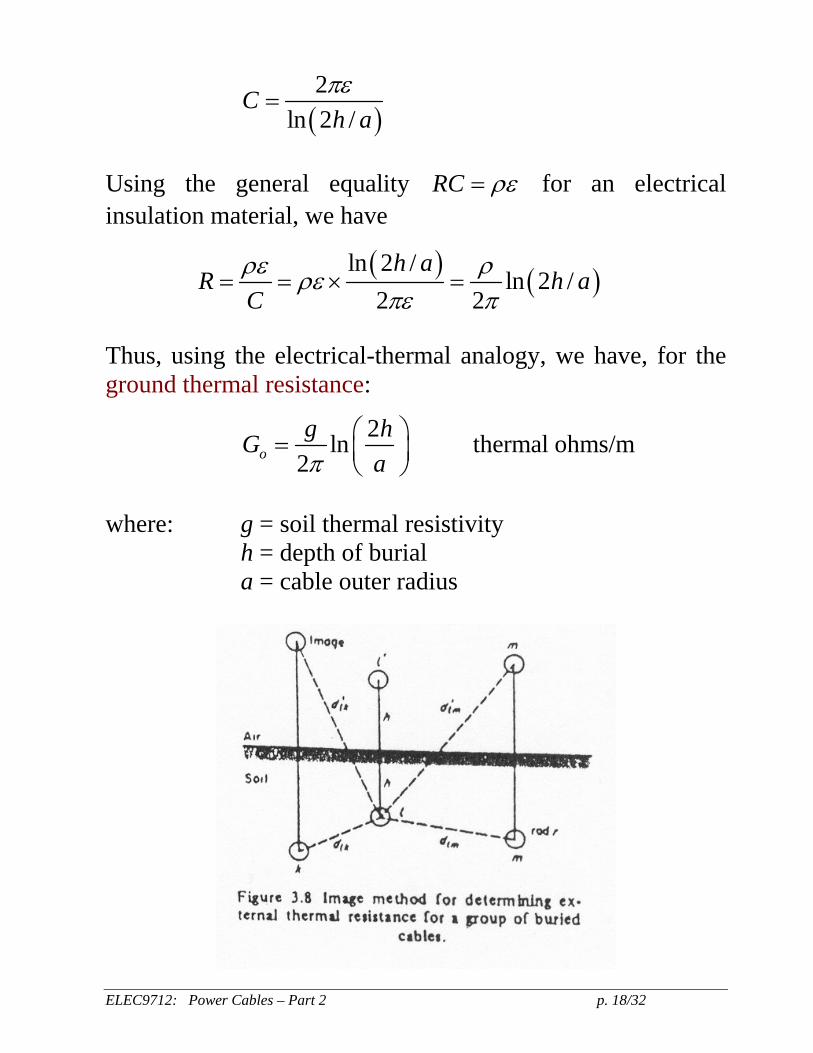
( )2
ln 2 /C
h aπε
=
Using the general equality RC ρε= for an electrical insulation material, we have
( ) ( )ln 2 /ln 2 /
2 2h a
R h aCρε ρρε
πε π= = × =
Thus, using the electrical-thermal analogy, we have, for the ground thermal resistance:
2ln thermal ohms/m2og hG
aπ⎛ ⎞= ⎜ ⎟⎝ ⎠
where: g = soil thermal resistivity h = depth of burial a = cable outer radius
ELEC9712: Power Cables – Part 2 p. 19/32
ELEC9712: Power Cables – Part 2 p. 20/32
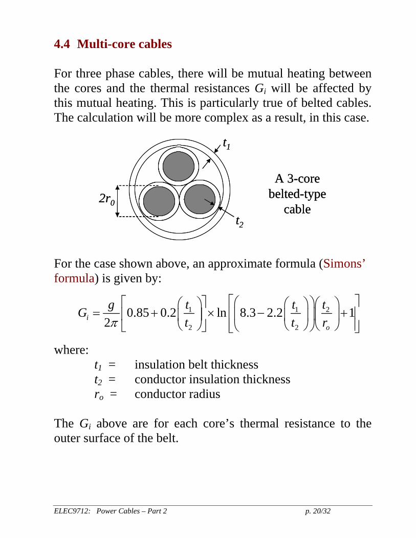
4.4 Multi-core cables For three phase cables, there will be mutual heating between the cores and the thermal resistances Gi will be affected by this mutual heating. This is particularly true of belted cables. The calculation will be more complex as a result, in this case.
t1
t2
2r0
A 3-corebelted-type
cable
t1
t2
2r0
A 3-corebelted-type
cable
For the case shown above, an approximate formula (Simons’ formula) is given by:
1 1 2
2 2
0.85 0.2 ln 8.3 2.2 12i
o
g t t tGt t rπ
⎡ ⎤⎡ ⎤ ⎛ ⎞⎛ ⎞⎛ ⎞ ⎛ ⎞= + × − +⎢ ⎥⎜ ⎟⎢ ⎥ ⎜ ⎟⎜ ⎟ ⎜ ⎟
⎢ ⎥⎝ ⎠ ⎝ ⎠ ⎝ ⎠⎣ ⎦ ⎝ ⎠⎣ ⎦
where: t1 = insulation belt thickness t2 = conductor insulation thickness ro = conductor radius
The Gi above are for each core’s thermal resistance to the outer surface of the belt.
ELEC9712: Power Cables – Part 2 p. 21/32
Gi
Gi Gb Gs
Gi
sheathGi
Gi Gb Gs
Gi
sheath
4.5 Cables in ducts For cables in ducts, an empirical expression is used, followed by iteration to get the rating.
( )1 m e
AGB CT D
=+ +
where:
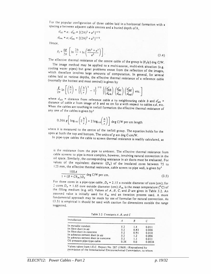
values of A, B and C are given in IEC 60287.
Tm is the mean temperature of the duct filling material
De is the equivalent diameter of the cores. [For a single core cable: De = OD of cable two cores cable: De = 1.65 x OD three core cable: De = 2.15 x OD ]
The thermal resistance is the thermal resistance between the pipe and the cable surfaces. The calculation procedure requires an initial educated guess of Tm and then iteration. Following is an example of a calculation by this method.
ELEC9712: Power Cables – Part 2 p. 22/32
Example: Determine the rating of a 500kV, 60Hz, three-phase oil pipe type cable buried in ground. The details are:
Pipe loss factor = 0.28 (eddy current loss) Conductor OD = 4.14 cm Insulation thickness = 3.40 cm Pipe diameter = 30 cm Burial depth = 100 cm Soil resistivity = 0.9 oC.m/W Ambient temperature = 25 oC AC resistance = 0.044 Ω/ph/km Insulation: g = 5.0 oC.m/W tanδ = 0.002 Tmax = 80 oC
Thermal resistance from pipe to cable is obtained from:
( )max1cp
e
AGB CT D
=+ +
where (from previous table) for an oil pressure pipe type cable: A = 0.26 ; B = 0 ; C = 0.0026 De = 2.15 x O.D. of core = 2.15 x (4.14 + 2 x 3.4) cm = 23.52 cm
ELEC9712: Power Cables – Part 2 p. 23/32
We take Tm as 55oC for first guess.
Then: ( )
0.261 0.0026 55 23.52cpG =
+ × ×
= 0.06 thermal Ω/m For the cable insulation:
5 23.52ln 0.772 4.14iGπ
⎛ ⎞= =⎜ ⎟⎝ ⎠
thermal Ω/m
For the ground:
0.9 2 100ln 0.372 15oGπ
×⎛ ⎞= =⎜ ⎟⎝ ⎠
thermal Ω/m
Thus the equivalent circuit is:
2ACI R
Gi
Go
TA= 25oC
0.772
ACI R0.77
2ACI R
0.77
80oC
0.370.06
Gcp
2ACI R
Gi
Go
TA= 25oC
0.772
ACI R0.77
2ACI R
0.77
80oC
0.370.06
Gcp
( )2 2 3 5 20.044 10 4.4 10ACI R I I− −= × × = × W/m/phase Pipe loss ( )5 23 0.28 4.4 10 I−= × × × W/m Dielectric loss: 2 tanoP CVω δ=
ELEC9712: Power Cables – Part 2 p. 24/32
but:
2 2004.14 3.4 3.4ln
4.14
C πε= =
+ +⎛ ⎞⎜ ⎟⎝ ⎠
pF/m/ph
hence:
( )23
12 500 10314 200 10 0.0023oP − ⎛ ⎞×
= × × × ×⎜ ⎟⎝ ⎠
W/m
10.47= W/m/core
80 25 55C AT T− = − = oC Hence:
( )( ) ( )( )5 2 5 255 4.4 10 0.77 3 4.4 10 0.06 0.37I I− −= × + × × +
( )0.7710.47 3 10.47 0.06 0.372
⎛ ⎞+ × + × × +⎜ ⎟⎝ ⎠
( )5 23 0.28 4.4 10 0.37I−+ × × × ×
i.e. 5 237.46 10.44 10 I−= × ⇒ 599I = A then use this to check Tm guess.
( ) ( )5 225 0.37 3 10.47 3 1 0.28 4.4 10 599mT −⎡ ⎤= + × + × + × × ×⎣ ⎦ = 25 + 34 = 62 oC [c.f. 55 oC] This is too high. Thus try Tm =58oC next and repeat until agreement is reached.
ELEC9712: Power Cables – Part 2 p. 25/32
5. Transient Heating of Cables When operated under non-steady state conditions, we can define three different transient ratings for cables. Because of the high thermal capacity of power cables, particularly when buried in the ground, these transient ratings are more relevant and more often used than the steady state rating determinations because of the long time constants associated with the cables. The three transient ratings used are:
(i) Short circuit rating: Determined from adiabatic heating of the cable under short circuit.
(ii) Cyclic rating: Determined using specified daily load cycles
(iii) Emergency Rating: Usually calculated for 1-2 hours of overload conditions 5.1 Short circuit rating This is calculated for a specified maximum (short circuit) temperature Tsc and a specified protection operating time (tsc) to clear the fault current. The equation previously quoted for adiabatic heating is used:
ELEC9712: Power Cables – Part 2 p. 26/32
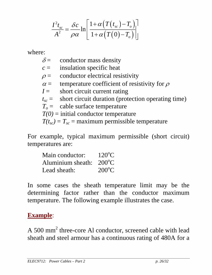
( )( )( )( )
2
2
1ln
1 0sc osc
o
T t TI t cA T T
αδρα α
⎡ ⎤+ −= ⎢ ⎥
+ −⎢ ⎥⎣ ⎦
where:
δ = conductor mass density c = insulation specific heat ρ = conductor electrical resistivity α = temperature coefficient of resistivity for ρ I = short circuit current rating tsc = short circuit duration (protection operating time) To = cable surface temperature T(0) = initial conductor temperature T(tsc) = Tsc = maximum permissible temperature
For example, typical maximum permissible (short circuit) temperatures are:
Main conductor: 120oC Aluminium sheath: 200oC Lead sheath: 200oC
In some cases the sheath temperature limit may be the determining factor rather than the conductor maximum temperature. The following example illustrates the case. Example: A 500 mm2 three-core Al conductor, screened cable with lead sheath and steel armour has a continuous rating of 480A for a
ELEC9712: Power Cables – Part 2 p. 27/32
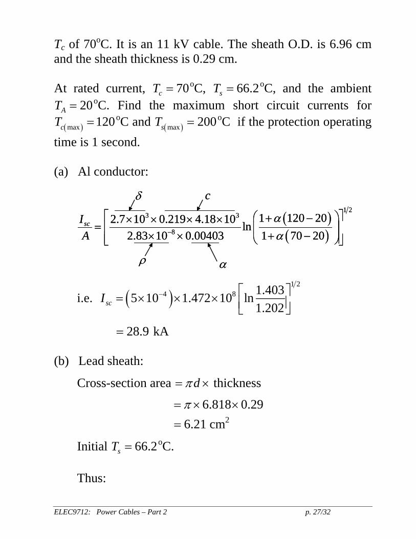
Tc of 70oC. It is an 11 kV cable. The sheath O.D. is 6.96 cm and the sheath thickness is 0.29 cm. At rated current, 70cT = oC, 66.2sT = oC, and the ambient
20AT = oC. Find the maximum short circuit currents for ( )max 120cT = oC and ( )max 200sT = oC if the protection operating
time is 1 second. (a) Al conductor:
( )( )
1 23 3
8
1 120 202.7 10 0.219 4.18 10 ln2.83 10 0.00403 1 70 20
scIA
αα−
⎡ ⎤⎛ ⎞+ −× × × ×= ⎢ ⎥⎜ ⎟
× × + −⎢ ⎥⎝ ⎠⎣ ⎦
δ c
αρ
( )( )
1 23 3
8
1 120 202.7 10 0.219 4.18 10 ln2.83 10 0.00403 1 70 20
scIA
αα−
⎡ ⎤⎛ ⎞+ −× × × ×= ⎢ ⎥⎜ ⎟
× × + −⎢ ⎥⎝ ⎠⎣ ⎦
δ c
αρ
i.e. ( )1 2
4 8 1.4035 10 1.472 10 ln1.202scI − ⎡ ⎤= × × × ⎢ ⎥⎣ ⎦
28.9= kA
(b) Lead sheath:
Cross-section area dπ= × thickness
6.818 0.29π= × ×
6.21= cm2
Initial 66.2sT = oC. Thus:
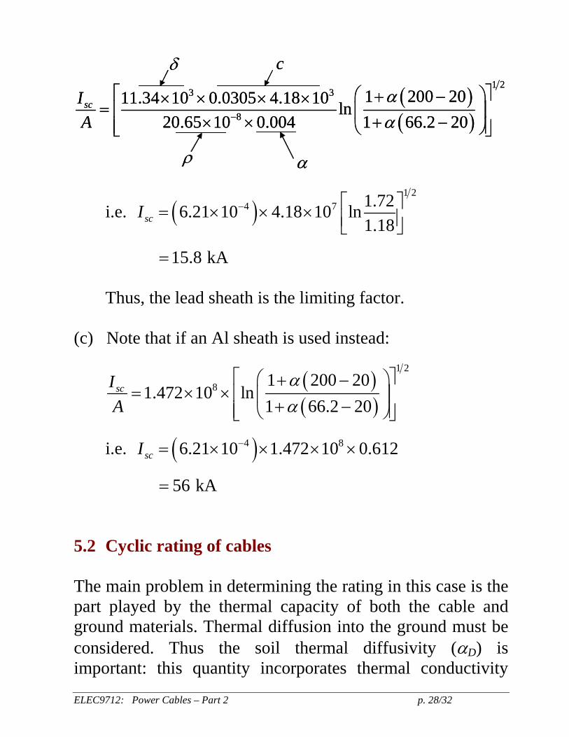
ELEC9712: Power Cables – Part 2 p. 28/32
( )( )
1 23 3
8
1 200 2011.34 10 0.0305 4.18 10 ln20.65 10 0.004 1 66.2 20
scIA
αα−
⎡ ⎤⎛ ⎞+ −× × × ×= ⎢ ⎥⎜ ⎟
× × + −⎢ ⎥⎝ ⎠⎣ ⎦
δ c
ρ α
( )( )
1 23 3
8
1 200 2011.34 10 0.0305 4.18 10 ln20.65 10 0.004 1 66.2 20
scIA
αα−
⎡ ⎤⎛ ⎞+ −× × × ×= ⎢ ⎥⎜ ⎟
× × + −⎢ ⎥⎝ ⎠⎣ ⎦
δ c
ρ α
i.e. ( )1 2
4 7 1.726.21 10 4.18 10 ln1.18scI − ⎡ ⎤= × × × ⎢ ⎥⎣ ⎦
15.8= kA Thus, the lead sheath is the limiting factor.
(c) Note that if an Al sheath is used instead:
( )( )
1 2
8 1 200 201.472 10 ln
1 66.2 20scIA
αα
⎡ ⎤⎛ ⎞+ −= × × ⎢ ⎥⎜ ⎟
+ −⎢ ⎥⎝ ⎠⎣ ⎦
i.e. ( )4 86.21 10 1.472 10 0.612scI −= × × × ×
56= kA 5.2 Cyclic rating of cables The main problem in determining the rating in this case is the part played by the thermal capacity of both the cable and ground materials. Thermal diffusion into the ground must be considered. Thus the soil thermal diffusivity (αD) is important: this quantity incorporates thermal conductivity
ELEC9712: Power Cables – Part 2 p. 29/32
(resistivity), density and specific heat of the soil: ( )D k cα δ= .
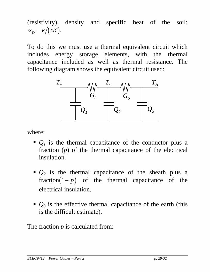
To do this we must use a thermal equivalent circuit which includes energy storage elements, with the thermal capacitance included as well as thermal resistance. The following diagram shows the equivalent circuit used:
Gi
Tc
Q3
Go
Ts TA
Q2Q1
Gi
Tc
Q3
Go
Ts TA
Q2Q1
where:
Q1 is the thermal capacitance of the conductor plus a fraction (p) of the thermal capacitance of the electrical insulation.
Q2 is the thermal capacitance of the sheath plus a fraction( )1 p− of the thermal capacitance of the electrical insulation.
Q3 is the effective thermal capacitance of the earth (this is the difficult estimate).
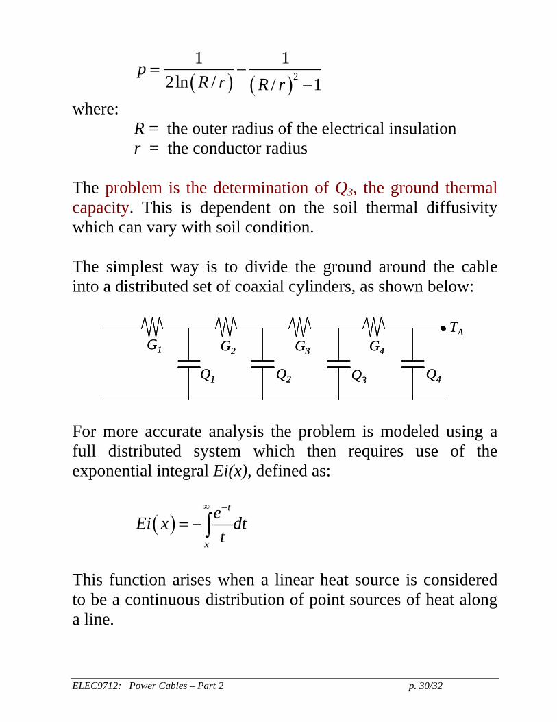
The fraction p is calculated from:
ELEC9712: Power Cables – Part 2 p. 30/32
( ) ( )21 1
2ln / / 1p
R r R r= −
−
where: R = the outer radius of the electrical insulation r = the conductor radius The problem is the determination of Q3, the ground thermal capacity. This is dependent on the soil thermal diffusivity which can vary with soil condition. The simplest way is to divide the ground around the cable into a distributed set of coaxial cylinders, as shown below:
G1
Q3
G2
TA
Q2Q1
G3 G4
Q4
G1
Q3
G2
TA
Q2Q1
G3 G4
Q4
For more accurate analysis the problem is modeled using a full distributed system which then requires use of the exponential integral Ei(x), defined as:
( )t
x
eEi x dtt
∞ −
= −∫
This function arises when a linear heat source is considered to be a continuous distribution of point sources of heat along a line.
ELEC9712: Power Cables – Part 2 p. 31/32
Using this function and the model of the cable and its mirror image, the cable surface temperature rise as a function of time is given by the equation:
( )2 2
4 16T
oD D
gW d hT t Ei Eit tπ α α
⎡ ⎤⎛ ⎞ ⎛ ⎞−= − + −⎢ ⎥⎜ ⎟ ⎜ ⎟
⎝ ⎠ ⎝ ⎠⎣ ⎦
plus any contributions from mutual heating by other cables where:
d = cable outer diameter h = burial depth WT = total losses per unit length g = soil thermal resistivity [ ]1 k= αD = soil thermal diffusivity ( )1 gcδ⎡ ⎤=⎣ ⎦ c = soil specific heat δ = soil mass density t = time 5.3 Emergency ratings Emergency ratings are determined for 1 or 2 hours of overload with the temperature of the insulation not to exceed the maximum limit. It is also complicated by the thermal diffusivity factor as with the cyclic rating. Emergency rating are an important consideration and are often used. The overload rating can be quite high because of
ELEC9712: Power Cables – Part 2 p. 32/32
the high thermal capacity and thermal diffusivity of the cable and surrounding ground.