electricity case: statistical analysis of electric power...

CREATE Research Archive

Published Articles & Papers

2005

Electricity Case: Statistical Analysis of ElectricPower OutagesJeffrey S. SimonoffNew York University

Carlos E. RestrepoNew York University, [email protected]

Rae ZimmermanNew York University, [email protected]

Wendy RemingtonNew York University, [email protected]

Lester B. LaveCarnegie Mellon University, [email protected]

See next page for additional authors

Follow this and additional works at: http://research.create.usc.edu/published_papers

This Article is brought to you for free and open access by CREATE Research Archive. It has been accepted for inclusion in Published Articles & Papersby an authorized administrator of CREATE Research Archive. For more information, please contact [email protected].

Recommended CitationSimonoff, Jeffrey S.; Restrepo, Carlos E.; Zimmerman, Rae; Remington, Wendy; Lave, Lester B.; Schuler, Richard E.; and Dooskin,Nicole, "Electricity Case: Statistical Analysis of Electric Power Outages" (2005). Published Articles & Papers. Paper 162.http://research.create.usc.edu/published_papers/162

http://research.create.usc.edu?utm_source=research.create.usc.edu%2Fpublished_papers%2F162&utm_medium=PDF&utm_campaign=PDFCoverPages

http://research.create.usc.edu/published_papers?utm_source=research.create.usc.edu%2Fpublished_papers%2F162&utm_medium=PDF&utm_campaign=PDFCoverPages

http://research.create.usc.edu/published_papers?utm_source=research.create.usc.edu%2Fpublished_papers%2F162&utm_medium=PDF&utm_campaign=PDFCoverPages

http://research.create.usc.edu/published_papers/162?utm_source=research.create.usc.edu%2Fpublished_papers%2F162&utm_medium=PDF&utm_campaign=PDFCoverPages

mailto:[email protected]

AuthorsJeffrey S. Simonoff, Carlos E. Restrepo, Rae Zimmerman, Wendy Remington, Lester B. Lave, Richard E.Schuler, and Nicole Dooskin

This article is available at CREATE Research Archive: http://research.create.usc.edu/published_papers/162

http://research.create.usc.edu/published_papers/162?utm_source=research.create.usc.edu%2Fpublished_papers%2F162&utm_medium=PDF&utm_campaign=PDFCoverPages

Electricity Case:

Statistical Analysis of Electric Power Outages

CREATE Report

Jeffrey S. Simonoff (NYU-Stern); Rae Zimmerman, Carlos E. Restrepo, Nicole J.

Dooskin, Ray V. Hartwell, Justin I. Miller and Wendy E. Remington (NYU-Wagner);

Lester B. Lave (Carnegie Mellon); Richard E. Schuler (Cornell)

New York University-Wagner Graduate School, Institute for Civil Infrastructure Systems

CREATE REPORT

Under Office of Naval Research Grant No. EMW-2004-GR-0112

July 26, 2005

Center for Risk and Economic Analysis of Terrorism Events University of Southern California

Los Angeles, CA

Report #05-013

This research was supported by the United States Department of Homeland Security through the Center for Risk and Economic Analysis of Terrorism Events (CREATE) under grant number EMW-2004-GR-0112. However, any opinions, findings, and conclusions or recommendations in this document are those of the authors and do not necessarily reflect

views of the United States Department of Homeland Security.

0

Electricity Case, Report 3

Electricity Case:

Statistical Analysis of Electric Power Outages

CREATE Report

July 26, 2005

Jeffrey S. Simonoff (NYU-Stern); Rae Zimmerman, Carlos E. Restrepo, Nicole J.

Dooskin, Ray V. Hartwell, Justin I. Miller and Wendy E. Remington (NYU-Wagner);

Lester B. Lave (Carnegie Mellon); Richard E. Schuler (Cornell)

New York University-Wagner Graduate School, Institute for Civil Infrastructure Systems

1

Abstract This report analyses electricity outages over the period January 1990-August 2004. A database was constructed using U.S. data from the DAWG database, which is maintained by the North American Electric Reliability Council (NERC). The data includes information about the date of the outage, geographical location, utilities affected, customers lost, duration of the outage in hours, and megawatts lost. Information found the DAWG database was also used to code the primary cause of the outage. Categories that included weather, equipment failure, human error, fires, and others were added to the database. In addition, information about the total number of customers served by the affected utilities, as well as total population and population density of the state affected in each incident, was incorporated to the database. The resulting database included information about 400 incidents over this period. The database was used to carry out two sets of analyses. The first is a set of analyses over time using three-, six-, or twelve-month averages for number of incidents, average outage duration, customers lost and megawatts lost. Negative binomial regression models, which account for overdispersion in the data, were used. For the number of incidents over time a seasonal analysis suggests there is a 9.7% annual increase in incident rate given season (that is, “holding season constant”) over this period. Given the year, summer is estimated to have 65-85% more incidents than the other seasons. The duration data suggest a more complicated trend; an analysis of duration per incident over time using a loess nonparametric regression “scatterplot smoother” suggests that between 1990-93 durations were getting shorter on average but this trend changed in the mid-1990s when average duration started to increase, and this increase became more pronounced after 2002. When looking at average customer losses by season there is weak evidence of an upward trend in the average customer loss per incident, with an estimated increase of a bit more than 10,000 customers per incident per year. Similar analyses of MW lost per incident over time showed no evidence of any time or seasonal patterns for this variable. The second part of the report includes a number of event-level analyses. The data in these analyses are modeled in two parts. First, the different characteristics related to whether an incident has zero or nonzero customers lost are determined. Then, given that the number lost is nonzero, the characteristics that help to predict the customers lost are analyzed. Unlike the first set of models described, in this section a number of predictors such as primary cause of the outage (including variables such as weather, equipment failure, system protection, human error and others), total number of customers served by the affected utilities, and the population density of the states where the outages occurred were used in the analyses to gain a better understanding of the three key outcome variables: customers lost, megawatts lost and duration of electric outages. Logistic regression was used in these analyses. For logged customers lost, the only predictor showing much of a relationship was logged MW lost. The total number of customers served by the utility was found to be a marginally significant predictor of customers lost per incident. Customer losses were higher for events caused by natural disaster, crime, unknown causes, and third party, and lower for incidents resulting from capacity shortage, demand reduction, and equipment failure, holding all else in the model fixed. The analyses for duration at the event level find that the two most common causes of outages, equipment failure and weather, are very different, with the former associated with shorter events and the latter associated with longer ones. When the primary cause of the events is included in the regression models, the time trend for the average duration per incident found in earlier analyses disappears. According to the data, weather related incidents are becoming more common in later years and equipment failures less common, and this change in the relative frequency of primary cause of the events accounts for much of the overall pattern of increasing average durations by season. Holding all else in the model constant, these analyses also suggest that winter events have an expected duration that is 2.25 times the duration of summer events, with autumn and spring in between. The event-level models can be used to construct predictions for outage outcomes based on different scenarios. We look at scenarios for New York, Chicago, San Francisco, and Seattle. Using the characteristics of the utilities in these four cities, the estimated expected duration and estimated expected customer loss (given nonzero loss) of an incident, separated by season and cause, can be determined for each city. We also construct 50% prediction intervals for duration and for customer loss (given that the loss is nonzero) for any cause and season for the four cities.

2

Acknowledgements

This research was supported by the United States Department of Homeland Security through the Center for Risk and Economic Analysis of Terrorism Events (CREATE), grant number EMW-2004-GR-0112. However, any opinions, findings, and conclusions or recommendations in this document are those of the author (s) and do not necessarily reflect views of the U.S. Department of Homeland Security.

3

Table of Contents Abstract and Acknowledgements 1

SUMMARY ANALYSES OVER TIME (pg. 4)

Analysis of the number of incidents over time 4 Analysis of the number of incidents that were associated with

nonzero MW loss or nonzero customer loss over time 12 Analysis of duration over time 18 Analysis of MW loss over time 29 Analysis of customer loss over time 34

EVENT-LEVEL ANALYSES (pg. 39)

Analysis of customer loss at the event level 39 Analysis of duration at the event level 54 Using the models for scenario prediction 64

APPENDIX (pg. 75)

Expected duration, probability of zero customer loss, and expected customer loss for different cities, seasons, and causes 75

REFERENCES (pg. 80)

4

Electricity Case: Statistical Analysis of Electric Power Outages This report presents the detailed results of the statistical analysis of electric power outage data summarized in the Electricity Case – Main Report. It contributes to the sections on the evaluation of risks and consequences of electric power outages. I. Summary analyses over time

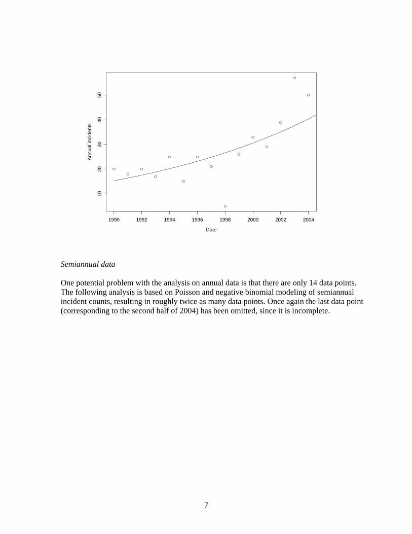
A. Analysis of the number of incidents over time This report summarizes the analyses of incident counts over time. Such count data are typically analyzed using special count regression models based on the Poisson and negative binomial distributions; see Simonoff (2003, chapter 5), for extensive discussion of these models. The standard count regression model is based on the Poisson distribution. The Poisson distribution has the property that its mean equals its variance, which can account for the observed pattern in count data that variability increases with level. Count regression models are generally fit as loglinear models; that is, it is the logarithm of the mean that is modeled as a linear function of predictors, or equivalently, the mean is modeled as an exponential function of the predictors. This implies, for example, a proportional relationship with a variable, rather than an additive one. Loglinear models are natural for count data because the true mean of the response cannot possibly be negative; a linear model on predictors can lead to estimated negative means, but a loglinear model cannot. Annual data We start with data measured at the annual level. The following is a plot of the annual incident figures for the U.S. data, along with the estimate of the time trend based on a Poisson regression model. Note that the estimated time trend is based only on years 1990 through 2003, since the 2004 data are incomplete (the data only run through August).

5

Date

Ann

ual i

ncid

ents

1990 1992 1994 1996 1998 2000 2002 2004

1020

3040

50

There are several noteworthy points here:

1. The fitted curve is consistent with an estimated annual increase in incidents of 8.2%. Note that it is apparent from the plot that a loglinear model is more reasonable than a linear model here, as the increase in incidents is slower in the 1990s than in the 2000s.

2. The estimated increase is highly significantly different from zero, with a Wald statistic (the analogue of a t-statistic for Poisson regression models) of 5.8. Here is output from the model detailing the significance testing based on the Poisson model: Coefficients: Value Std. Error Wald (Intercept) -153.6724123 27.2931301 -5.630443 Date 0.0785583 0.0136619 5.750174 The significance of the time trend can be assessed by calculating a tail probability for the 5.75 based on a normal distribution; in this case it is zero to 8 digits. The estimated annual increase in incidents comes from exponentiating the slope coefficient in this model, as exp(.0786) = 1.082, implying an estimated 8.2% annual increase.

3. The year 1998 was obviously a very unusual one, with a very small number of incidents (5, where the model implies an estimate of 26.0).

4. There is evidence that the incident rate is increasing in recent years. The model implies an estimated 39.6 incidents in 2003, when there were, in fact, 57 (this is roughly 2 ¾

6

standard deviations above the expected number), and an estimated 42.9 in 2004, when there were 50 in only the first 8 months of the year. The 2003 number is apparently not because of the August 14, 2003 blackout, since that event only accounts for 8 incidents.

There is a flaw in this analysis, in that the Poisson regression model does not fit the data well, because of overdispersion. Overdispersion occurs when there is unmodeled heterogeneity in the data. The Poisson model treats each year as identical, other than the actual difference in year. This is unlikely to be true, as the chances are very good that there have been many changes to the structure of power generation over the years (new power plants come on line, old ones go off, new drains on power generation occur, political situations change, and so on). The Poisson model does not account for this possibility, and as a result the observed variability in the response is larger than that implied by the Poisson model (recall that the Poisson distribution has the property that the mean equals the variance). An important result of overdispersion is that the statistical significance of effects in the model are overstated.

Overdispersion has occurred here, as both the Pearson (X2=34.1) and deviance (G2=42.0, both on 12 degrees of freedom) goodness-of-fit statistics indicate that the Poisson model does not fit the data.

A way of addressing overdispersion is to fit a count regression model that allows for the variance being larger than the mean. The standard model of this type is the negative binomial regression model. Here is output for this model:

Coefficients: Value Std. Error Wald (Intercept) -135.76307835 47.91257415 -2.833558 Date 0.06959082 0.02399384 2.900362

The Wald statistic for this model is smaller than in the Poisson model, but it is still highly significant (p=.002). The model fits the data well, as the deviance equals 15.3 on 12 degrees of freedom (p=.23, not rejecting the fit of the model). The estimated annual increase in incidents based on this model is slightly lower than before, implying a 7.2% annual increase in incidents. Here is a graphical representation of the estimated trend:

7

Date

Ann

ual i

ncid

ents

1990 1992 1994 1996 1998 2000 2002 2004

1020

3040

50

Semiannual data One potential problem with the analysis on annual data is that there are only 14 data points. The following analysis is based on Poisson and negative binomial modeling of semiannual incident counts, resulting in roughly twice as many data points. Once again the last data point (corresponding to the second half of 2004) has been omitted, since it is incomplete.

8

Date

Sem

iann

ual i

ncid

ents

1990 1992 1994 1996 1998 2000 2002 2004

010

2030

40

This analysis reinforces and refines some of the earlier impressions. 1. The implications regarding the increase in incidents are similar for these semiannual data

to those for the annual data. The estimated rate of increase is 9.5% annually, similar to what was seen before.

2. The estimated increase is even more significantly different from zero, with a Wald statistic of 7.1. Here is output for the model:


3. We can see from the plot that it was the second half of 1998 that was so unusual, with only 1 incident (and 14.1 predicted by the model).

4. The first part of 2003 actually had fewer incidents than expected; it was the 46 incidents in the second half of 2003 (more than twice the expected number) that was so unusual. Again, only eight of these were from the August 14 blackout. The first half of 2004 was a bit above normal, but not overwhelmingly so, but the 18 incidents in the first two months of the second half of 2004 is noticeably high. Thus, in addition to the relatively stable annual increase in incidents, there is still (limited) evidence of an increasing rate recently.

5. There is evidence of overdispersion in these data as well, as the Pearson (X2=87.2) and deviance (G2=92.4, both on 27 degrees of freedom) indicate lack of fit. A negative binomial fit to these data is as follows:

9

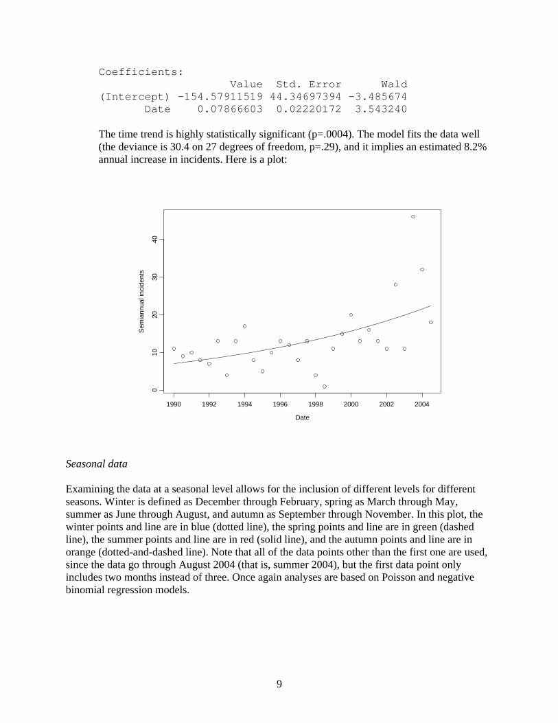
Coefficients: Value Std. Error Wald (Intercept) -154.57911519 44.34697394 -3.485674 Date 0.07866603 0.02220172 3.543240 The time trend is highly statistically significant (p=.0004). The model fits the data well (the deviance is 30.4 on 27 degrees of freedom, p=.29), and it implies an estimated 8.2% annual increase in incidents. Here is a plot:

Date

Sem

iann

ual i

ncid

ents

1990 1992 1994 1996 1998 2000 2002 2004

010

2030

40

Seasonal data Examining the data at a seasonal level allows for the inclusion of different levels for different seasons. Winter is defined as December through February, spring as March through May, summer as June through August, and autumn as September through November. In this plot, the winter points and line are in blue (dotted line), the spring points and line are in green (dashed line), the summer points and line are in red (solid line), and the autumn points and line are in orange (dotted-and-dashed line). Note that all of the data points other than the first one are used, since the data go through August 2004 (that is, summer 2004), but the first data point only includes two months instead of three. Once again analyses are based on Poisson and negative binomial regression models.

10

Date

Inci

dent

s by

sea

son

1990 1992 1994 1996 1998 2000 2002 2004

05

1015

20

1. Taking the season into account, the estimated annual increase in incident rate is 10.6%. All of the estimates obtained thus far are within the estimated standard errors of each other, so from a statistical point of view, all are equally reasonable. That is, what is most reasonable is to say is that the estimated increase in incidents is roughly 7-10% annually.

2. This increase is highly statistically significantly different from zero (Wald statistic 8.0). Here is output; the tests for the seasons take Autumn as a baseline category.

Coefficients: Value Std. Error Wald (Intercept) -199.65377545 25.23546760 -7.9116337 Date 0.10076407 0.01262495 7.9813418 SeasonSpring 0.09030258 0.15677222 0.5760114 SeasonSummer 0.57368747 0.14186760 4.0438230 SeasonWinter 0.06404012 0.15980743 0.4007330

3. While the winter, spring, and autumn estimated rates are similar to each other (with autumn having a rate that is slightly lower), summer has a noticeably (and statistically significantly) higher rate of incidents. This is presumably from weather effects: snow and ice in the winter, thunderstorms in parts of the US in spring, and most importantly thunderstorms and intense heat (with corresponding air conditioner use) in the summer (and the lack of all of these factors in the autumn; we might have expected evidence of a hurricane effect in autumn, but only Hurricane Floyd in 1999 and Hurricane Isabel in 2003 show up as noteworthy). The difference between the summer rate and that of the other seasons is highly statistically significant, but more importantly, corresponds to an important effect in practical terms, since the estimated number of incidents is 60% to 80% higher in summer than in the other seasons, given the year.

11

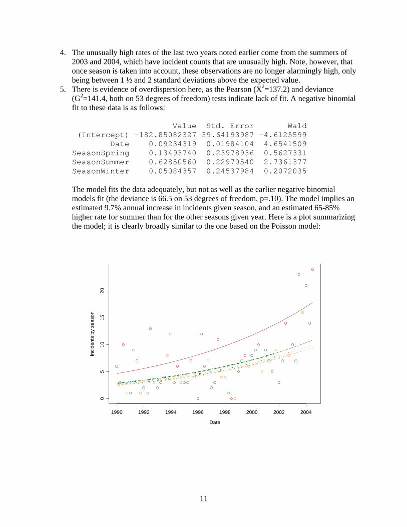
4. The unusually high rates of the last two years noted earlier come from the summers of 2003 and 2004, which have incident counts that are unusually high. Note, however, that once season is taken into account, these observations are no longer alarmingly high, only being between 1 ½ and 2 standard deviations above the expected value.

5. There is evidence of overdispersion here, as the Pearson (X2=137.2) and deviance (G2=141.4, both on 53 degrees of freedom) tests indicate lack of fit. A negative binomial fit to these data is as follows: Value Std. Error Wald (Intercept) -182.85082327 39.64193987 -4.6125599 Date 0.09234319 0.01984104 4.6541509 SeasonSpring 0.13493740 0.23978936 0.5627331 SeasonSummer 0.62850560 0.22970540 2.7361377 SeasonWinter 0.05084357 0.24537984 0.2072035 The model fits the data adequately, but not as well as the earlier negative binomial models fit (the deviance is 66.5 on 53 degrees of freedom, p=.10). The model implies an estimated 9.7% annual increase in incidents given season, and an estimated 65-85% higher rate for summer than for the other seasons given year. Here is a plot summarizing the model; it is clearly broadly similar to the one based on the Poisson model:

Date

Inci

dent

s by

sea

son

1990 1992 1994 1996 1998 2000 2002 2004

05

1015

20

12

B. Analysis of the number of incidents that were associated with nonzero MW loss or nonzero customer loss over time The earlier analyses included incidents where there was no effect on the customer base, either in terms of customers affected or power loss. It could be argued that it is incidents that affect customers that are most interesting, so this portion of the report focuses on those incidents alone, excluding events with zero customers lost. Overdispersion occurs in all of the models, so all analyses are based on the negative binomial model. 1. INCIDENTS WITH NONZERO MW LOST Annual data Here is a plot with the negative binomial fit superimposed.

Date

Ann

ual i

ncid

ents

1990 1992 1994 1996 1998 2000 2002 2004

1020

3040

50

Here is output for this model:


13

The strength of the time trend is weaker than for the complete data, having a tail probability of .044. The estimated annual increase in incidents with nonzero MW is exp(.058295)-1=6.0%, so apparently the incidents with zero MW lost inflated the rate slightly (since this rate, with those incidents omitted, is smaller than the rate estimated based on all incidents). Note that 1998 is still unusually low, and 2003 and 2004 are unusually high. Semiannual data Here is a plot with the fitted model on the semiannual data.

Date

Sem

iann

ual i

ncid

ents

1990 1992 1994 1996 1998 2000 2002 2004

010

2030

40

Here is output for the model: Coefficients: Value Std. Error Wald (Intercept) -151.48640808 54.82831060 -2.762923 Date 0.07694855 0.02744971 2.803256 The estimated annual increase in incidents with nonzero MW loss is 8.0%, and is highly significant (p=.005). Note that while the second half of 2003 and of 2004 (only two months) are still high, now the first half of 2003 is also very high (this is because all of the incidents in the first half of 2003 were nonzero MW loss incidents).

14

Seasonal data Here is a plot by season.

Date

Inci

dent

s by

sea

son

1990 1992 1994 1996 1998 2000 2002 2004

05

1015

20

The fit to these data is as follows: Coefficients: Value Std. Error Wald (Intercept) -189.77487351 49.48534232 -3.8349714 Date 0.09555951 0.02476742 3.8582754 SeasonSpring 0.32805162 0.30244169 1.0846772 SeasonSummer 0.84044230 0.29118948 2.8862385 SeasonWinter 0.20764577 0.31001341 0.6697961 The model implies an estimated 10.0% annual increase in incident rate given season, which is highly statistically significant (p<.0001), and an estimated 65-130% higher rate for summer than for the other seasons. The summer effect is stronger than before, which is easy to understand: while more than 90% of the summer incidents had nonzero MW loss, roughly ¼ of the incidents in the autumn had zero MW loss. That is, nonzero MW incidents are more likely in the summer, thereby strengthening the “summer effect” here. In terms of the time trend, we see a similar pattern to before, of a 6-10% annual increase in incidents from the analyses based on the three different time aggregations.

15

2. INCIDENTS WITH NONZERO CUSTOMERS LOST Annual data Here is a plot with the negative binomial fit superimposed.

Date

Ann

ual i

ncid

ents

1990 1992 1994 1996 1998 2000 2002 2004

1020

3040

50

Here is output for this model:

Coefficients: Value Std. Error Wald (Intercept) -191.83850183 69.27401101 -2.769271 Date 0.09745008 0.03469084 2.809101 The strength of the time trend is stronger than for the analysis based only on nonzero MW incidents, having a tail probability of .005. The estimated annual increase in incidents with nonzero customer loss is exp(.09745)-1=10.2%, so apparently the incidents with zero customers lost deflated the rate earlier (the rate is higher once the zero customer loss events are omitted). This makes sense: the rate of incidents that had no customer loss was more than 35% from 1990-1997, but has been only 7.5% since then. Note that 1998 is not unusually low now, but 2003 and 2004 are still unusually high.

16

Semiannual data Here is a plot with the fitted model on the semiannual data.

Date

Sem

iann

ual i

ncid

ents

1990 1992 1994 1996 1998 2000 2002 2004

010

2030

40

Here is output for the model: Coefficients: Value Std. Error Wald (Intercept) -219.3758662 59.57344642 -3.682444 Date 0.1108936 0.02982306 3.718385 The estimated annual increase in incidents with nonzero MW loss is 11.7%, and is highly statistically significant (p=.0002). The second half of 2003 and first half of 2004 are unusually high.

17

Seasonal data Here is a plot of the seasonal data.

Date

Inci

dent

s by

sea

son

1990 1992 1994 1996 1998 2000 2002 2004

05

1015

20

The fit to these data is as follows: Coefficients: Value Std. Error Wald (Intercept) -261.5615113 52.93962548 -4.9407511 Date 0.1314558 0.02649295 4.9619145 SeasonSpring 0.2818310 0.31959945 0.8818255 SeasonSummer 0.8567975 0.30630300 2.7972219 SeasonWinter 0.1727073 0.32699348 0.5281674 The model implies an estimated 14.0% annual increase in incident rate (p zero to six digits), and an estimated 75-135% higher rate for summer than for the other seasons. The summer effect is similar to that for the nonzero MW loss data, but the pattern is a little more complicated: both summer and winter have lower rates of incidents with zero customer loss compared to spring and autumn, so the estimated relative chances of incidents in those seasons compared to spring and autumn are now higher. Overall, while removing the zero MW loss incidents has relatively little effect on the estimated annual increase in incident rate, removing the zero customer loss incidents has a stronger effect on the estimated annual increase of rates, increasing it to 12-14%.

18

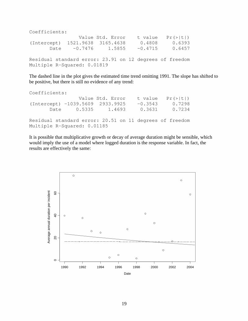
C. Analysis of duration over time We now discuss the pattern of average duration of incidents over time. The response variable, whether measured annually, semiannually, or seasonally, is the average duration per incident over that time period. Note that zero-loss events are included, since they seem to be directly relevant to an analysis of duration. Obviously, events with missing duration are not included, which raises the issue of nonresponse bias. If the incidents for which duration is missing are different from those in which it was reported, that can bias the results in ways that are impossible to ascertain. Annual data We start with analyses based on a linear model for durations. Here is a plot of the average duration versus time, with two lines superimposed.

Date

Ave

rage

ann

ual d

urat

ion

per i

ncid

ent

1990 1992 1994 1996 1998 2000 2002 2004

020

4060

It is apparent that there is little evidence of any time trend in average duration. There is one early outlier, corresponding to 1991, although it is not that different from the values for 2003 and 2004. The solid line is the fitted time trend of average duration based on all of the data other than 2004 (since those data were incomplete), which has a negative slope that is far from statistically significant:

19

Coefficients: Value Std. Error t value Pr(>|t|) (Intercept) 1521.9638 3165.4638 0.4808 0.6393 Date -0.7476 1.5855 -0.4715 0.6457 Residual standard error: 23.91 on 12 degrees of freedom Multiple R-Squared: 0.01819 The dashed line in the plot gives the estimated time trend omitting 1991. The slope has shifted to be positive, but there is still no evidence of any trend: Coefficients: Value Std. Error t value Pr(>|t|) (Intercept) -1039.5609 2933.9925 -0.3543 0.7298 Date 0.5335 1.4693 0.3631 0.7234 Residual standard error: 20.51 on 11 degrees of freedom Multiple R-Squared: 0.01185 It is possible that multiplicative growth or decay of average duration might be sensible, which would imply the use of a model where logged duration is the response variable. In fact, the results are effectively the same:

Date

Ave

rage

ann

ual d

urat

ion

per i

ncid

ent

1990 1992 1994 1996 1998 2000 2002 2004

020

4060

20

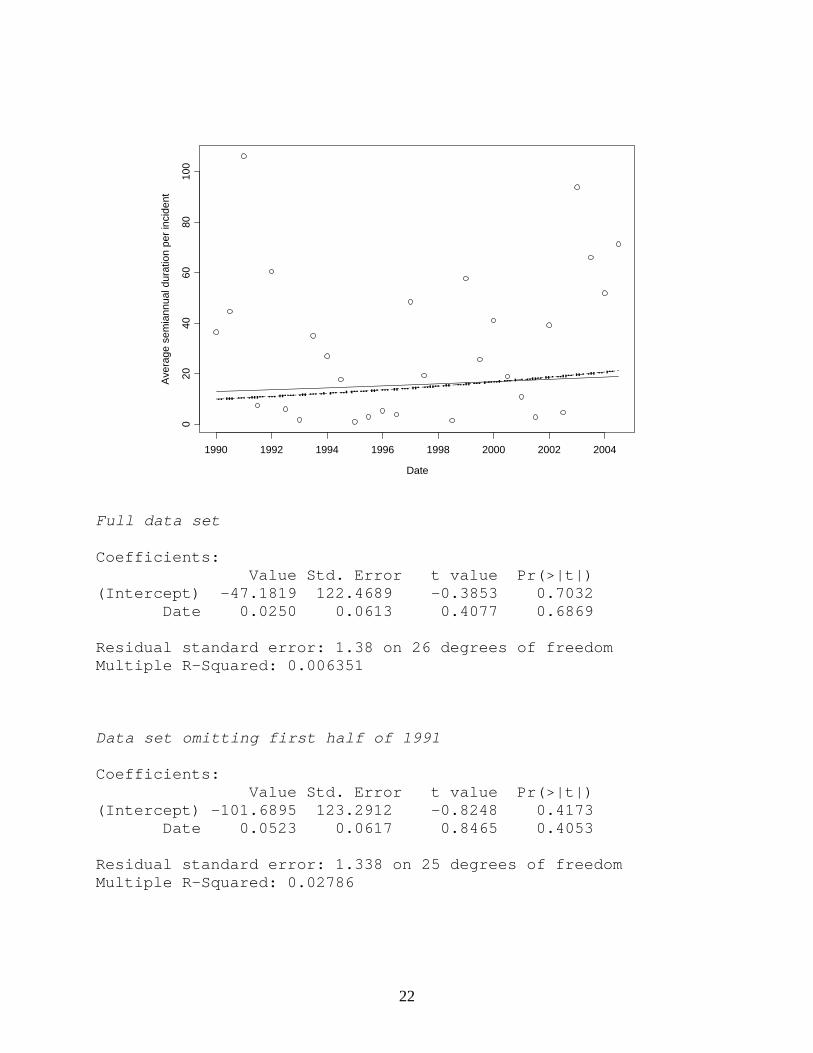
Full data set Coefficients: Value Std. Error t value Pr(>|t|) (Intercept) 77.8956 165.8329 0.4697 0.6470 Date -0.0376 0.0831 -0.4522 0.6592 Residual standard error: 1.253 on 12 degrees of freedom Multiple R-Squared: 0.01675 Data set omitting 1991 Coefficients: Value Std. Error t value Pr(>|t|) (Intercept) 4.3909 177.7861 0.0247 0.9807 Date -0.0008 0.0890 -0.0089 0.9930 Residual standard error: 1.243 on 11 degrees of freedom Multiple R-Squared: 7.267e-006 Semiannual data Here is a plot of the semiannual data, with linear trend lines superimposed.

Date

Ave

rage

sem

iann

ual d

urat

ion

per i

ncid

ent

1990 1992 1994 1996 1998 2000 2002 2004

020

4060

8010

0

21

The results are similar to those for the annual data. The estimated time trend is slightly positive when the 1991 time period is included, and slightly negative when it is not included, but in neither case is it close to statistical significance. Note that the value for the second half of 2004 is not included in either model, since the data are incomplete for that time period. Here is computer output for the two models: Full data set Coefficients: Value Std. Error t value Pr(>|t|) (Intercept) -857.6518 2569.1990 -0.3338 0.7412 Date 0.4445 1.2865 0.3455 0.7325 Residual standard error: 28.95 on 26 degrees of freedom Multiple R-Squared: 0.004569 Data set omitting first half of 1991 Coefficients: Value Std. Error t value Pr(>|t|) (Intercept) -2933.8052 2246.1745 -1.3061 0.2034 Date 1.4825 1.1247 1.3182 0.1994 Residual standard error: 24.37 on 25 degrees of freedom Multiple R-Squared: 0.06499 Models for logged duration also find no evidence of any effect:

22

Date

Aver

age

sem

iann

ual d

urat

ion

per i

ncid

ent

1990 1992 1994 1996 1998 2000 2002 2004

020

4060

8010

0

Full data set Coefficients: Value Std. Error t value Pr(>|t|) (Intercept) -47.1819 122.4689 -0.3853 0.7032 Date 0.0250 0.0613 0.4077 0.6869 Residual standard error: 1.38 on 26 degrees of freedom Multiple R-Squared: 0.006351 Data set omitting first half of 1991 Coefficients: Value Std. Error t value Pr(>|t|) (Intercept) -101.6895 123.2912 -0.8248 0.4173 Date 0.0523 0.0617 0.8465 0.4053 Residual standard error: 1.338 on 25 degrees of freedom Multiple R-Squared: 0.02786

23

Seasonal data Here is a plot based on all of the data other than the first data point, fitting a linear time trend.

Date

Ave

rage

dur

atio

n pe

r inc

iden

t by

seas

on

1990 1992 1994 1996 1998 2000 2002 2004

050

100

150

There is a slight upward slope, but it is not statistically significant. There is also no evidence of a season effect; the autumn line is marginally lower than the other lines, but this is not close to significance. Coefficients: Value Std. Error t value Pr(>|t|) (Intercept) -1875.0749 2771.2612 -0.6766 0.5021 Date 0.9484 1.3874 0.6836 0.4978 SeasonSpring 19.8532 17.4212 1.1396 0.2605 SeasonSummer 17.1705 17.4189 0.9857 0.3295 SeasonWinter 19.9349 18.4376 1.0812 0.2854 Residual standard error: 43.23 on 45 degrees of freedom Multiple R-Squared: 0.04553 F-statistic: 0.5366 on 4 and 45 degrees of freedom, the p-value is 0.7095 Anova Table Response: Duration Sum Sq Df F value Pr(>F) (Intercept) 855.66 1 0.4578069 0.5021140 Date 873.34 1 0.4672694 0.4977509

24

Season 3135.53 3 0.5592066 0.6447021 Residuals 84106.52 45 The summer 1993 point is unusual, so here is a summary omitting that data point.

Date

Ave

rage

dur

atio

n pe

r inc

iden

t by

seas

on

1990 1992 1994 1996 1998 2000 2002 2004

050

100

150

There is now (very) weak evidence of an upward slope, but no season effect. This is presumably coming from the last six seasons, wherein four had average durations of more than 60 hours. Coefficients: Value Std. Error t value Pr(>|t|) (Intercept) -3285.2832 2313.1906 -1.4202 0.1626 Date 1.6544 1.1581 1.4286 0.1602 SeasonSpring 19.9999 14.4166 1.3873 0.1723 SeasonSummer 4.6768 14.6619 0.3190 0.7513 SeasonWinter 19.7584 15.2577 1.2950 0.2021 Residual standard error: 35.78 on 44 degrees of freedom Multiple R-Squared: 0.1011 F-statistic: 1.237 on 4 and 44 degrees of freedom, the p-value is 0.3091 Anova Table Response: Duration Sum Sq Df F value Pr(>F) Sum Sq Df F value Pr(>F) (Intercept) 2581.72 1 2.017079 0.1625856 Date 2612.13 1 2.040840 0.1601858

25

Season 3820.00 3 0.994847 0.4041244 Residuals 56316.96 44 The increasing trend in the last few data points suggests that a model for logged duration based on seasonal data might be appropriate, since in such a model while the proportional increase in duration is constant over time, the absolute level increases more quickly as time goes on (assuming that the slope is positive).

Date

Ave

rage

Dur

atio

n lo

st p

er in

cide

nt b

y se

ason

1990 1992 1994 1996 1998 2000 2002 2004

050

100

150

The time trend is statistically significant, but there is no season effect. For this reason, the solid black line (the estimated time trend not including a season effect) is added to the plot. Coefficients: Value Std. Error t value Pr(>|t|) (Intercept) -239.2458 107.6682 -2.2221 0.0314 Date 0.1207 0.0539 2.2389 0.0302 SeasonSpring 0.6486 0.6768 0.9583 0.3430 SeasonSummer 0.9567 0.6768 1.4137 0.1643 SeasonWinter 0.9926 0.7163 1.3856 0.1727 Residual standard error: 1.68 on 45 degrees of freedom Multiple R-Squared: 0.1458 F-statistic: 1.92 on 4 and 45 degrees of freedom, the p-value is 0.1235

26

Anova Table Response: log(Duration) Sum Sq Df F value Pr(>F) (Intercept) 13.9300 1 4.937573 0.031350 Date 14.1414 1 5.012505 0.030155 Season 7.2384 3 0.855231 0.471228 Residuals 126.9551 45 Omitting season effect Coefficients: Value Std. Error t value Pr(>|t|) (Intercept) -240.8782 107.1072 -2.2489 0.0291 Date 0.1218 0.0536 2.2721 0.0276 Residual standard error: 1.672 on 48 degrees of freedom Multiple R-Squared: 0.0971 F-statistic: 5.162 on 1 and 48 degrees of freedom, the p-value is 0.0276 This corresponds to an estimated annual increase in duration of 13.0% (exp(.1218)=1.1295). The summer of 1993 is unusual, so here is the analysis with that point omitted:

Date

Aver

age

Dur

atio

n lo

st p

er in

cide

nt b

y se

ason

1990 1992 1994 1996 1998 2000 2002 2004

050

100

150

27

Coefficients: Value Std. Error t value Pr(>|t|) (Intercept) -265.4906 105.5836 -2.5145 0.0157 Date 0.1338 0.0529 2.5316 0.0150 SeasonSpring 0.6513 0.6580 0.9898 0.3277 SeasonSummer 0.7242 0.6692 1.0822 0.2851 SeasonWinter 0.9893 0.6964 1.4205 0.1625 Residual standard error: 1.633 on 44 degrees of freedom Multiple R-Squared: 0.1662 F-statistic: 2.193 on 4 and 44 degrees of freedom, the p-value is 0.08532 Anova Table Response: log(Duration) Sum Sq Df F value Pr(>F) (Intercept) 16.8602 1 6.322745 0.0156500 Date 17.0907 1 6.409193 0.0150001 Season 5.8621 3 0.732782 0.5380322 Residuals 117.3300 44 Omitting season effect Coefficients: Value Std. Error t value Pr(>|t|) (Intercept) -267.9718 104.5487 -2.5631 0.0136 Date 0.1354 0.0523 2.5863 0.0129 Residual standard error: 1.619 on 47 degrees of freedom Multiple R-Squared: 0.1246 This model implies an estimated annual increase in duration of 14.5%. We also can note that the observed average durations in the last 7 seasons (winter 2003 through summer 2004) are all higher than what is implied by the model. That is, what the multiplicative model is picking up, which the linear model cannot pick up, is an increase in durations in the last few years. This is supported when noting that the average duration up through autumn 2002 was 28.4 hours, while the average duration after that was 69.0 hours. Further, the corresponding medians are 10.4 hours and 63.8 hours. A more precise representation of this pattern comes from the following plot, which is a loess nonparametric curve for the durations. This is a nonparametric regression “scatterplot smoother,” which puts a smooth curve through the points, thereby avoiding the linear or loglinear assumptions made in the parametric statistical models. Details on nonparametric regression can be found in Simonoff (1996, chapter 5).

28

The loess curve implies that average durations dropped in the first few years of the 1990s. After a period of relatively flat durations, the average duration first started to increase in the mid 1990s, and then increased more rapidly after 2002.

Date

Aver

age

Dur

atio

n lo

st p

er in

cide

nt b

y se

ason

1990 1992 1994 1996 1998 2000 2002 2004

050

100

150

It is possible to get estimates of the local annual rates of change of duration from this curve. These estimates have subtle statistical properties, so they should only be considered guidelines, but they do give a feel for what is going on. Here are the estimated annual changes in duration: 1991 -0.47688186 1992 -0.32825299 1993 -0.14540827 1994 0.14093464 1995 0.50430449 1996 0.84530415 1997 0.35273835 1998 0.17398574 1999 0.11282195 2000 0.00913204 2001 0.13988508 2002 0.26066940 2003 0.48978316 Up until 1993, durations were getting shorter on average (an estimated 48% shorter from 1991 to 1992, 33% shorter from 1992 to 1993, and so on). This changed in 1994, and for a few years the average duration went up 35-85% annually (note that this was at a time when durations were lower, so the absolute increase wasn’t that large). This was followed by a period (1998-2001) of fairly stable growth of 10-20% annually (with growth in 2000 less than that). Finally, from 2002

29

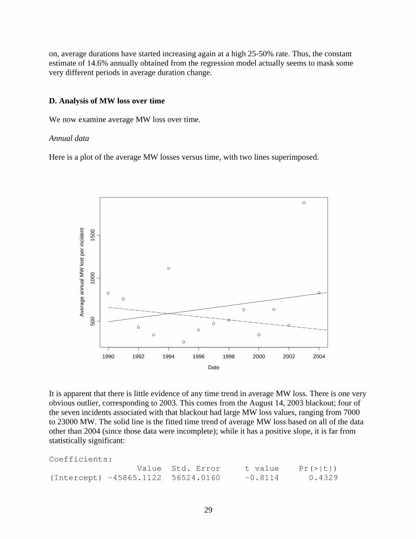
on, average durations have started increasing again at a high 25-50% rate. Thus, the constant estimate of 14.6% annually obtained from the regression model actually seems to mask some very different periods in average duration change. D. Analysis of MW loss over time We now examine average MW loss over time. Annual data Here is a plot of the average MW losses versus time, with two lines superimposed.

Date

Ave

rage

ann

ual M

W lo

st p

er in

cide

nt

1990 1992 1994 1996 1998 2000 2002 2004

500

1000

1500

It is apparent that there is little evidence of any time trend in average MW loss. There is one very obvious outlier, corresponding to 2003. This comes from the August 14, 2003 blackout; four of the seven incidents associated with that blackout had large MW loss values, ranging from 7000 to 23000 MW. The solid line is the fitted time trend of average MW loss based on all of the data other than 2004 (since those data were incomplete); while it has a positive slope, it is far from statistically significant: Coefficients: Value Std. Error t value Pr(>|t|) (Intercept) -45865.1122 56524.0160 -0.8114 0.4329

30

Date 23.2969 28.3115 0.8229 0.4266 Residual standard error: 427 on 12 degrees of freedom Multiple R-Squared: 0.05341 The dashed line in the plot gives the estimated time trend omitting 2003. The slope has shifted to be negative, but there is still no evidence of any real trend: Coefficients: Value Std. Error t value Pr(>|t|) (Intercept) 36925.3025 35110.5655 1.0517 0.3155 Date -18.2229 17.5904 -1.0360 0.3225 Residual standard error: 237.3 on 11 degrees of freedom Multiple R-Squared: 0.08889 Semiannual data Here is a plot of the semiannual data, with trend lines superimposed.

Date

Ave

rage

sem

iann

ual M

W lo

st p

er in

cide

nt

1990 1992 1994 1996 1998 2000 2002 2004

050

010

0015

0020

00

The results are similar to those for the annual data. The estimated time trend is slightly positive when the August 2003 blackout time period is included, and slightly negative when it is not

31

included, but in neither case is it close to statistical significance. Note that the unusually high value for the second half of 2004 is not included in either model, since the data are incomplete for that time period. Here is computer output for the two models: Full data set Coefficients: Value Std. Error t value Pr(>|t|) (Intercept) -13163.5432 37887.7200 -0.3474 0.7310 Date 6.8844 18.9723 0.3629 0.7195 Residual standard error: 427.4 on 27 degrees of freedom Multiple R-Squared: 0.004853 Data set omitting second half of 2003 Coefficients: Value Std. Error t value Pr(>|t|) (Intercept) 31910.7556 26878.7923 1.1872 0.2459 Date -15.7170 13.4611 -1.1676 0.2536 Residual standard error: 289.9 on 26 degrees of freedom Multiple R-Squared: 0.04982 Seasonal data Here is a plot based on all of the data (other than the first data point, which was not based on a full three months of a season).

32

Date

Ave

rage

MW

lost

per

inci

dent

by

seas

on

1990 1992 1994 1996 1998 2000 2002 2004

010

0020

0030

00

There is a slight upward slope, but it is not statistically significant. There is also no evidence of a season effect; the summer line is marginally significantly higher than the autumn line, but this difference is not close to significance if all of the pairwise comparisons between seasons that can be made are taken into account. Coefficients: Value Std. Error t value Pr(>|t|) (Intercept) -40041.5623 38282.5274 -1.0459 0.3005 Date 20.2187 19.1693 1.0547 0.2965 SeasonSpring 94.3449 228.7118 0.4125 0.6817 SeasonSummer 463.5128 232.4624 1.9939 0.0515 SeasonWinter 348.0473 232.5976 1.4963 0.1407 Residual standard error: 603.5 on 51 degrees of freedom Multiple R-Squared: 0.1129 F-statistic: 1.622 on 4 and 51 degrees of freedom, the p-value is 0.183 Anova Table Response: MW Sum Sq Df F value Pr(>F) (Intercept) 398439 1 1.094009 0.3005168 Date 405167 1 1.112483 0.2965141 Season 1921266 3 1.758432 0.1668606 Residuals 18574233 51

33

The summer 2003 point is highly unusual, so a summary omitting that data point follows.

Date

Aver

age

MW

lost

per

inci

dent

by

seas

on

1990 1992 1994 1996 1998 2000 2002 2004

010

0020

0030

00

There is even less evidence of any effect, as summer is no different from winter, and the slope is virtually flat. Coefficients: Value Std. Error t value Pr(>|t|) (Intercept) -1951.8292 29765.8421 -0.0656 0.9480 Date 1.1457 14.9047 0.0769 0.9390 SeasonSpring 98.0128 173.9725 0.5634 0.5757 SeasonSummer 251.6850 180.1201 1.3973 0.1685 SeasonWinter 356.4834 176.9325 2.0148 0.0493 Residual standard error: 459 on 50 degrees of freedom Multiple R-Squared: 0.08881 F-statistic: 1.218 on 4 and 50 degrees of freedom, the p-value is 0.3149 Anova Table Response: MW Sum Sq Df F value Pr(>F) (Intercept) 906 1 0.004300 0.9479794 Date 1245 1 0.005909 0.9390329 Season 1024037 3 1.619850 0.1965117 Residuals 10536339 50 Thus, there is no evidence of any time or seasonal patterns in average MW loss per incident.

34

E. Analysis of customer loss over time Annual data Here is a plot of the average customer losses versus time, with two lines superimposed.

Date

Ave

rage

ann

ual C

usto

mer

s lo

st p

er in

cide

nt

1990 1992 1994 1996 1998 2000 2002 2004

5000

010

0000

1500

0020

0000

2500

0030

0000

It is apparent that there is little evidence of any time trend in average customer loss. I’ve also included the trend omitting 2003, although that year doesn’t really show up as outlying with respect to customer loss; in any event, that only make the time trend less significant. Here is computer output: Full data set Coefficients: Value Std. Error t value (Intercept) -11476942.2686 12761932.1574 -0.8993 Date 5828.8956 6392.1393 0.9119 Pr(>|t|) (Intercept) 0.3862

35

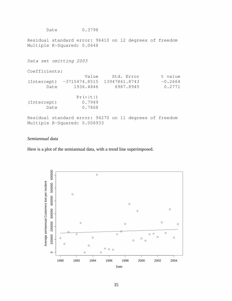
Date 0.3798 Residual standard error: 96410 on 12 degrees of freedom Multiple R-Squared: 0.0648 Data set omitting 2003 Coefficients: Value Std. Error t value (Intercept) -3715474.8515 13947861.8743 -0.2664 Date 1936.4846 6987.8945 0.2771 Pr(>|t|) (Intercept) 0.7949 Date 0.7868 Residual standard error: 94270 on 11 degrees of freedom Multiple R-Squared: 0.006933 Semiannual data Here is a plot of the semiannual data, with a trend line superimposed.

Date

Ave

rage

sem

iann

ual C

usto

mer

s lo

st p

er in

cide

nt

1990 1992 1994 1996 1998 2000 2002 2004

010

0000

2000

0030

0000

4000

0050

0000

6000

00

36

The results are similar to those for the annual data, in that there is a slight positive slope, but not close to statistical significance. Coefficients: Value Std. Error t value (Intercept) -3718770.1426 12534458.3895 -0.2967 Date 1944.1571 6276.6304 0.3097 Pr(>|t|) (Intercept) 0.7690 Date 0.7591 Residual standard error: 141400 on 27 degrees of freedom Multiple R-Squared: 0.003541 Seasonal data Here is a plot of the data.

Date

Ave

rage

Cus

tom

ers

lost

per

inci

dent

by

seas

on

1990 1992 1994 1996 1998 2000 2002 2004

05*

10^5

10^6

1.5*

10^6

It is apparent that there is no evidence of either a time or season effect.

37

Coefficients: Value Std. Error t value (Intercept) -13669781.7516 14595904.6082 -0.9365 Date 6911.4549 7307.2262 0.9458 SeasonSpring -24317.4782 87934.2329 -0.2765 SeasonSummer 16233.1520 87924.0146 0.1846 SeasonWinter 81139.2433 89370.0144 0.9079 Pr(>|t|) (Intercept) 0.3533 Date 0.3486 SeasonSpring 0.7832 SeasonSummer 0.8542 SeasonWinter 0.3681 Residual standard error: 232000 on 52 degrees of freedom Multiple R-Squared: 0.04681 F-statistic: 0.6385 on 4 and 52 degrees of freedom, the p-value is 0.6374 Anova Table Response: Customers Sum Sq Df F value Pr(>F) (Intercept) 47221822505 1 0.8771243 0.3533200 Date 48163215547 1 0.8946102 0.3486056 Season 86900927084 3 0.5380486 0.6583191 Residuals 2799528926494 52 Winter 1995 is evidently unusual (there was only one incident where customer loss was recorded, and it was 1.5 million customers). Omitting that point from the model fitting now highlights a time effect. The season lines are dashed in the following picture. There is now an upward slope, and it is statistically significant. There is no evidence of a season effect.

38

Date

Aver

age

Cus

tom

ers

lost

per

inci

dent

by

seas

on

1990 1992 1994 1996 1998 2000 2002 2004

05*

10^5

10^6

1.5*

10^6

Coefficients: Value Std. Error t value (Intercept) -20658490.3354 8688786.2747 -2.3776 Date 10406.8580 4349.8834 2.3924 Season1 -11822.6427 26085.4891 -0.4532 Season2 9284.7123 14697.3116 0.6317 Season3 -4304.7448 10903.2789 -0.3948 Pr(>|t|) (Intercept) 0.0212 Date 0.0205 Season1 0.6523 Season2 0.5304 Season3 0.6946 Residual standard error: 137700 on 51 degrees of freedom Multiple R-Squared: 0.1137 F-statistic: 1.636 on 4 and 51 degrees of freedom, the p-value is 0.1795

39

Anova Table Response: Customers Sum Sq Df F value Pr(>F) (Intercept) 107127706057 1 5.652999 0.0212125 Date 108469312202 1 5.723794 0.0204587 Season 14856817016 3 0.261325 0.8529158 Residuals 966480393522 51 These results suggest simplifying the model by removing the season factor, and this single line is the black line in the figure. Here is output for this model: Coefficients: Value Std. Error t value (Intercept) -20710107.4567 8502707.6973 -2.4357 Date 10432.8078 4256.7412 2.4509 Pr(>|t|) (Intercept) 0.0182 Date 0.0175 Residual standard error: 134800 on 54 degrees of freedom Multiple R-Squared: 0.1001 Thus, when looking at average customer losses season by season, there is weak evidence of an upward trend in the average customer loss per incident, with an estimated increase of a bit more than 10,000 customers per incident per year. The effect is weak, accounting for only 10% in the variability of average customer losses. Looking at the plot, it seems that this effect is being driven by the lack of points in the lower right corner; that is, the lack of very low customer loss events in the past 5 years, compared to pre-1999. This coincides with the pattern noted in sections I. A and I. B when comparing the trend of the number of incidents over time to the number of incidents with nonzero customer loss over time. In those analyses, it was apparent that the number of zero customer loss incidents has dropped significantly since 1999, which could account for the increase in average customer loss seen here. II. Event-level analyses

A. Analysis of customer loss at the event level In this section customer loss is reanalyzed, but now at the event level. There are two important distinctions between these analyses and those of section I. E. First, the earlier analyses were based on average customer losses over three- six- or twelve-month time periods, and as such there is far lower variability in the responses than for the event-by-event customer losses. Second, the present analyses can account for characteristics unique to the particular event through regression modeling, while the earlier analyses ignored those characteristics.

40

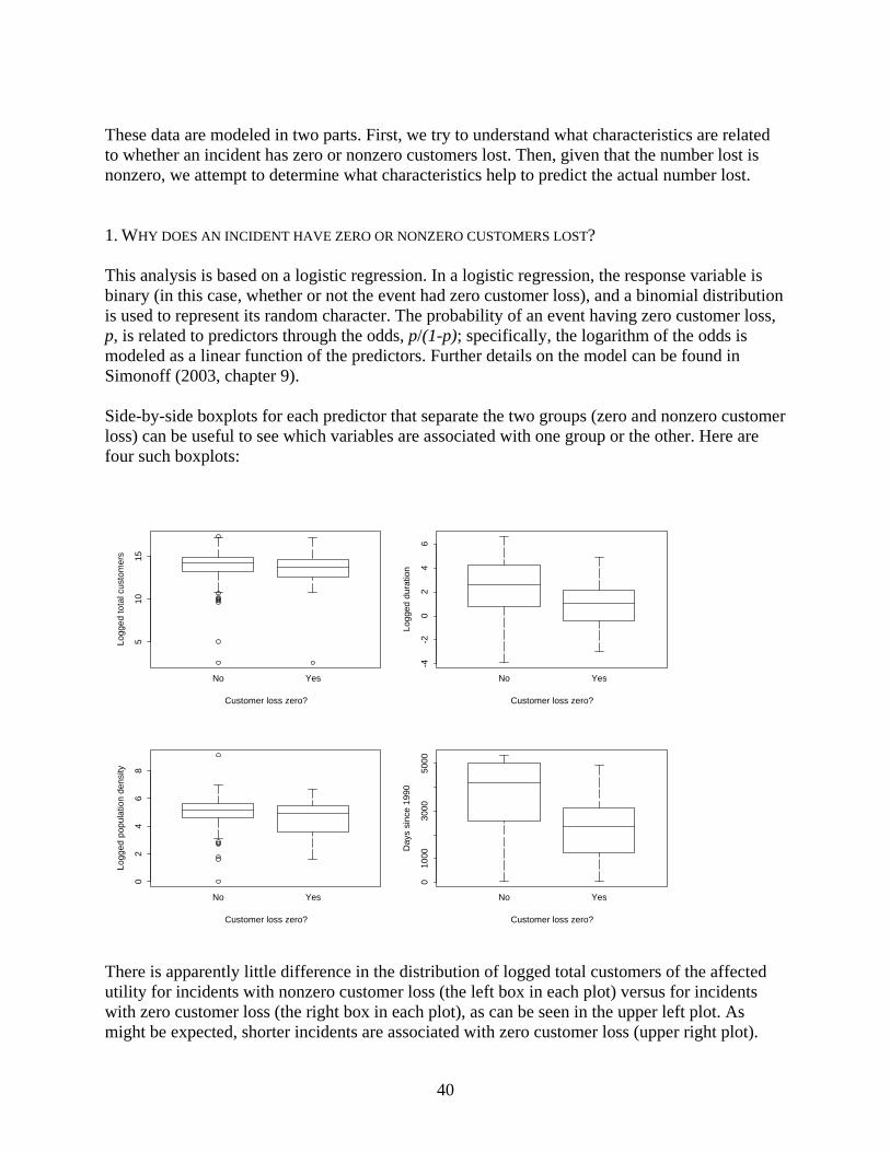
These data are modeled in two parts. First, we try to understand what characteristics are related to whether an incident has zero or nonzero customers lost. Then, given that the number lost is nonzero, we attempt to determine what characteristics help to predict the actual number lost. 1. WHY DOES AN INCIDENT HAVE ZERO OR NONZERO CUSTOMERS LOST? This analysis is based on a logistic regression. In a logistic regression, the response variable is binary (in this case, whether or not the event had zero customer loss), and a binomial distribution is used to represent its random character. The probability of an event having zero customer loss, p, is related to predictors through the odds, p/(1-p); specifically, the logarithm of the odds is modeled as a linear function of the predictors. Further details on the model can be found in Simonoff (2003, chapter 9). Side-by-side boxplots for each predictor that separate the two groups (zero and nonzero customer loss) can be useful to see which variables are associated with one group or the other. Here are four such boxplots:

510

15

No Yes

Customer loss zero?

Logg

ed to

tal c

usto

mer

s

-4-2

02

46

No Yes

Customer loss zero?

Logg

ed d

urat

ion

02

46

8

No Yes

Customer loss zero?

Logg

ed p

opul

atio

n de

nsity

010

0030

0050

00

No Yes

Customer loss zero?

Day

s si

nce

1990

There is apparently little difference in the distribution of logged total customers of the affected utility for incidents with nonzero customer loss (the left box in each plot) versus for incidents with zero customer loss (the right box in each plot), as can be seen in the upper left plot. As might be expected, shorter incidents are associated with zero customer loss (upper right plot).

41

Incidents in more densely populated states are more likely to have nonzero customer loss (bottom left plot). Finally, as noted in the earlier time trend analyses of incident rates and customer loss, there is a strong pattern where incidents earlier in time are more likely to have zero customer loss (bottom right plot). The other potential predictors are season and cause. The following table summarizes the marginal relationship with season: Winter Spring Summer Autumn Nonzero loss 62 60 111 48 Zero loss 10 21 20 13 Zero loss incidents are more common in the spring (26.3%) and autumn (21.3%), and less common in the summer (15.3%) and winter (13.9%). These are not, however, very strong effects. The cause of the incident is also a potentially important predictor of the seriousness of the event. The following table gives the catalogued causes for the incidents, along with the codes used for them in the output and figures to follow.

Cause Code Capacity shortage C Crime Crime Demand reduction D Equipment failure E Fire F Human error H Operational error O Natural disaster N System protection S Third party T Unknown U Weather W

Table 1. Causes of incidents with codes.

The following table summarizes the relationship between the occurrence of zero or nonzero customer loss and cause of the incident: C Crime D E F H N O S T U W Nonzero loss 6 2 1 63 7 10 2 3 4 2 7 173 Zero loss 1 6 3 26 4 7 1 2 0 3 1 8 Weather-related incidents (W) are very likely to have nonzero customer loss. Capacity shortage (C), system protection (S), and unknown causes (U) are also strongly associated with nonzero customer loss, but this is based on far fewer incidents. Equipment failure (E) is noticeably less related to nonzero customer loss (while also having a large number of incidents). More atypical causes that are less associated with nonzero customer loss include fire (F), human error (H),

42

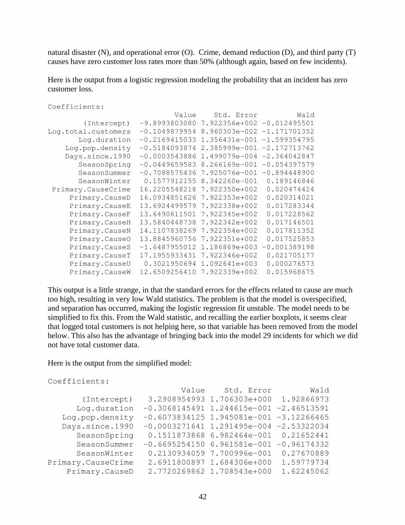
natural disaster (N), and operational error (O). Crime, demand reduction (D), and third party (T) causes have zero customer loss rates more than 50% (although again, based on few incidents). Here is the output from a logistic regression modeling the probability that an incident has zero customer loss. Coefficients: Value Std. Error Wald (Intercept) -9.8993803080 7.922356e+002 -0.012495501 Log.total.customers -0.1049879954 8.960303e-002 -1.171701352 Log.duration -0.2169415033 1.356431e-001 -1.599354795 Log.pop.density -0.5184093874 2.385999e-001 -2.172713762 Days.since.1990 -0.0003543886 1.499079e-004 -2.364042847 SeasonSpring -0.0449659583 8.266169e-001 -0.054397579 SeasonSummer -0.7088575436 7.925076e-001 -0.894448900 SeasonWinter 0.1577912155 8.342260e-001 0.189146846 Primary.CauseCrime 16.2205548218 7.922350e+002 0.020474424 Primary.CauseD 16.0934851626 7.922353e+002 0.020314021 Primary.CauseE 13.6924499579 7.922338e+002 0.017283344 Primary.CauseF 13.6490611501 7.922345e+002 0.017228562 Primary.CauseH 13.5840448738 7.922342e+002 0.017146501 Primary.CauseN 14.1107838269 7.922354e+002 0.017811352 Primary.CauseO 13.8845960756 7.922351e+002 0.017525853 Primary.CauseS -1.6487955012 1.186869e+003 -0.001389198 Primary.CauseT 17.1955933431 7.922346e+002 0.021705177 Primary.CauseU 0.3021950694 1.092641e+003 0.000276573 Primary.CauseW 12.6509256410 7.922339e+002 0.015968675 This output is a little strange, in that the standard errors for the effects related to cause are much too high, resulting in very low Wald statistics. The problem is that the model is overspecified, and separation has occurred, making the logistic regression fit unstable. The model needs to be simplified to fix this. From the Wald statistic, and recalling the earlier boxplots, it seems clear that logged total customers is not helping here, so that variable has been removed from the model below. This also has the advantage of bringing back into the model 29 incidents for which we did not have total customer data. Here is the output from the simplified model: Coefficients: Value Std. Error Wald (Intercept) 3.2908954993 1.706303e+000 1.92866973 Log.duration -0.3068145491 1.244615e-001 -2.46513591 Log.pop.density -0.6073834125 1.945081e-001 -3.12266465 Days.since.1990 -0.0003271641 1.291495e-004 -2.53322034 SeasonSpring 0.1511873868 6.982464e-001 0.21652441 SeasonSummer -0.6695254150 6.961581e-001 -0.96174332 SeasonWinter 0.2130934059 7.700996e-001 0.27670889 Primary.CauseCrime 2.6911800897 1.684306e+000 1.59779734 Primary.CauseD 2.7720269862 1.708543e+000 1.62245062

43

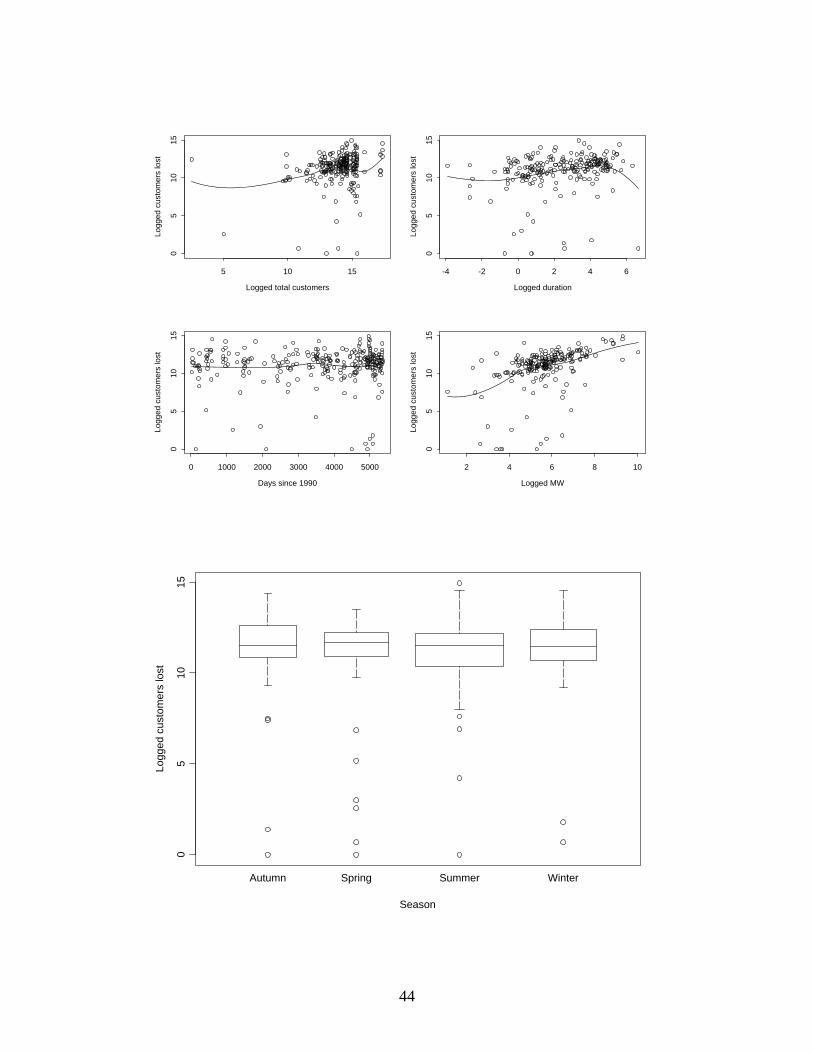
Primary.CauseE -0.2664512138 1.194480e+000 -0.22306882 Primary.CauseF -0.1170414575 1.441739e+000 -0.08118077 Primary.CauseH -0.5060062221 1.380445e+000 -0.36655308 Primary.CauseN 0.4467313019 1.973418e+000 0.22637437 Primary.CauseO -1.1496985596 1.773590e+000 -0.64823260 Primary.CauseS -13.9244551234 3.204103e+002 -0.04345821 Primary.CauseT 3.0384818062 1.672036e+000 1.81723427 Primary.CauseU 0.1401502460 1.695997e+000 0.08263589 Primary.CauseW -1.7355275486 1.257502e+000 -1.38013937 Tests for terms with more than 1 degree of freedom Term Chi-Square DF P Season 2.5385 3 0.468 Primary.Cause 28.5179 11 0.003 We see that logged duration, logged population density, a time trend (days since 1990), and cause are significant predictors, but season is not. The coefficients have the following interpretations. A 1% increase in the duration of an incident is associated with an estimated 0.3% decrease in the odds that an incident will have zero customer loss, holding all else in the model fixed. A 1% increase in the state population density is associated with an estimated 0.6% decrease in the odds that an incident will have zero customer loss, holding all else in the model fixed. Since exp(365 X -.0003271641)=.887, each additional year later is associated with an estimated 11.3% decrease in the odds that an incident has zero customer loss, holding all else in the model fixed (that is, the estimated annual decrease in the odds of an event having zero customer loss is 11.3%, holding all else in the model fixed). Finally, given the other predictors, crime, demand reduction, and third party cause are strongly associated with zero customer loss, while operational error, system protection, and weather are strongly associated with nonzero loss. 2. GIVEN THAT MORE THAN ZERO CUSTOMERS ARE LOST, WHAT FACTORS ARE RELATED TO THE AMOUNT LOST? We now examine regression modeling for the (logged) number of customers lost, given that that number is nonzero. First, here are some pictures of the observed relationships, with loess curves superimposed on the plots.

44

Logged total customers

Logg

ed c

usto

mer

s lo

st

5 10 15

05

1015

Logged duration

Logg

ed c

usto

mer

s lo

st

-4 -2 0 2 4 6

05

1015

Days since 1990

Logg

ed c

usto

mer

s lo

st

0 1000 2000 3000 4000 5000

05

1015

Logged MW

Logg

ed c

usto

mer

s lo

st

2 4 6 8 10

05

1015

05

1015

Autumn Spring Summer Winter

Season

Logg

ed c

usto

mer

s lo

st

45

05

1015

C CrimeD E F H N O S T U W

Primary cause

Logg

ed c

usto

mer

s lo

st

The only potential predictor showing much of a relationship with logged customers lost is logged MW loss. There is little evident seasonal effect. There is a primary cause effect, however, with fire, natural disaster, weather, and especially unknown causes having generally higher customer losses, and capacity shortage, operational error, and system protection having smaller losses. Note that these boxplots have been constructed so that the width of the box is proportional to the square root of the sample size for that group, so the wider the box, the more information there is for that group. It is evident that most incidents are either weather-related, or due to equipment failure. A least squares regression implies that only logged MW is a significant predictor, but there is extreme nonconstant variance related to primary cause. Df Sum of Sq Mean Sq F Value Pr(F) Log.MW 1 67.7417 67.74171 17.05755 0.0000591 Log.duration 1 3.1032 3.10323 0.78140 0.3780820 Log.pop.density 1 0.0025 0.00249 0.00063 0.9800483 Log.total.customers 1 5.1732 5.17319 1.30262 0.2554946 Primary.Cause 10 24.4770 2.44770 0.61634 0.7983204 Season 3 4.8571 1.61902 0.40767 0.7477002 Days.since.1990 1 2.4502 2.45015 0.61696 0.4333798 Residuals 155 615.5610 3.97136 Here are side-by-side boxplots of the residuals separated by cause, which illustrates the nonconstant variance. Note that there is much higher variability in the residuals from the

46

regression model for some causes than for others. This invalidates the inferences from the ordinary least squares model.

-10

-8-6

-4-2

02

4

C Crime D E F H N O S T U W

Primary cause

Sta

ndar

dize

d re

sidu

als

Weighted least squares (WLS) is used to correct for the nonconstant variance. In a WLS analysis, the events from causes with less variability, such as capacity shortage and fire, are weighted higher, while those from causes with more variability, such as equipment failure and system protection, are weighted lower. Here is output for the WLS model. Df Sum of Sq Mean Sq F Value Pr(F) Log.MW 1 33.4173 33.41728 32.49694 0.0000001 Log.duration 1 0.2267 0.22668 0.22044 0.6393648 Log.pop.density 1 0.0177 0.01770 0.01722 0.8957766 Log.total.customers 1 3.9135 3.91349 3.80571 0.0528816 Primary.Cause 10 15.5513 1.55513 1.51230 0.1396358 Season 3 1.0843 0.36143 0.35148 0.7881295 Days.since.1990 1 2.8564 2.85637 2.77771 0.0976045 Residuals 155 159.3898 1.02832 The (logged) MW effect is by far the strongest effect. The total number of customers served by the utility is also a (marginally) significant predictor of the customers lost. There is weak evidence of a time trend (p=.098), and weaker evidence of an effect related to cause (p=.14). Here is output for the model:

47

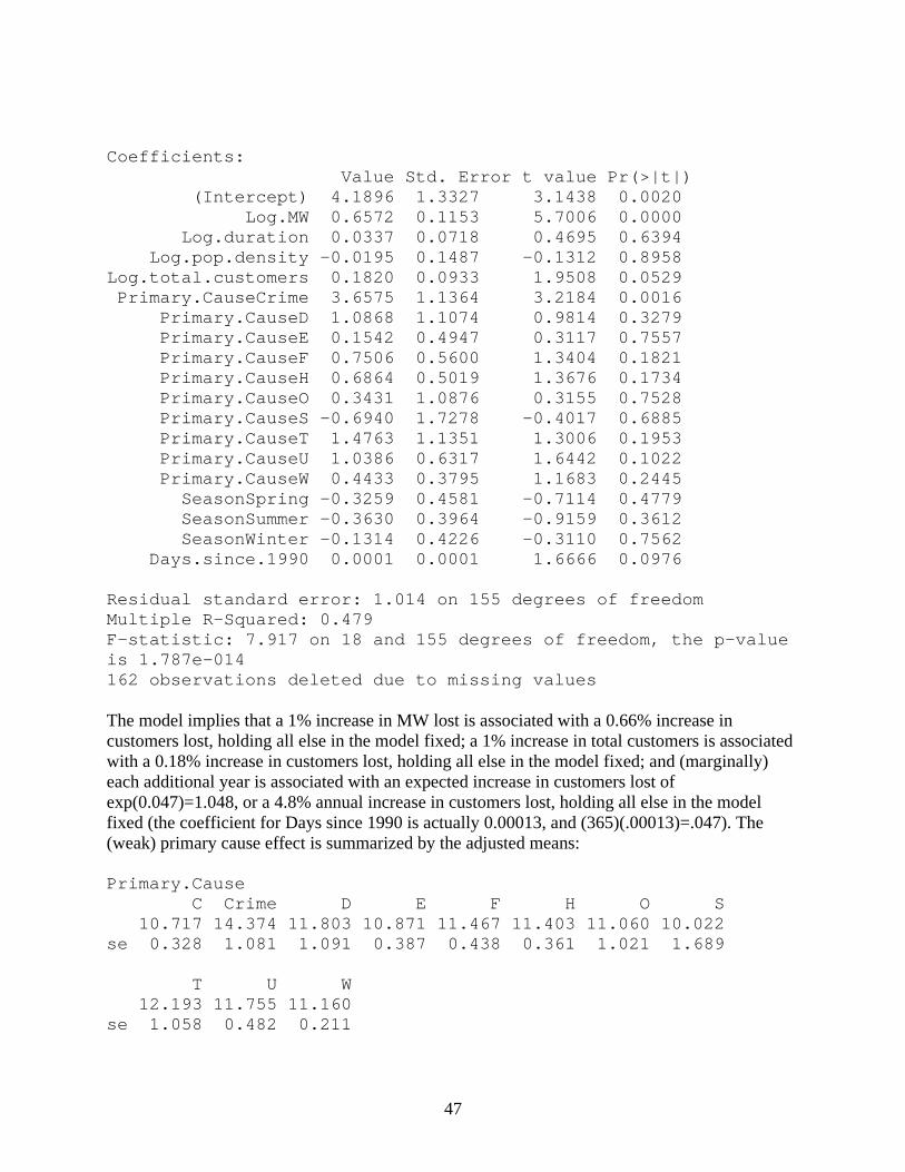
Coefficients: Value Std. Error t value Pr(>|t|) (Intercept) 4.1896 1.3327 3.1438 0.0020 Log.MW 0.6572 0.1153 5.7006 0.0000 Log.duration 0.0337 0.0718 0.4695 0.6394 Log.pop.density -0.0195 0.1487 -0.1312 0.8958 Log.total.customers 0.1820 0.0933 1.9508 0.0529 Primary.CauseCrime 3.6575 1.1364 3.2184 0.0016 Primary.CauseD 1.0868 1.1074 0.9814 0.3279 Primary.CauseE 0.1542 0.4947 0.3117 0.7557 Primary.CauseF 0.7506 0.5600 1.3404 0.1821 Primary.CauseH 0.6864 0.5019 1.3676 0.1734 Primary.CauseO 0.3431 1.0876 0.3155 0.7528 Primary.CauseS -0.6940 1.7278 -0.4017 0.6885 Primary.CauseT 1.4763 1.1351 1.3006 0.1953 Primary.CauseU 1.0386 0.6317 1.6442 0.1022 Primary.CauseW 0.4433 0.3795 1.1683 0.2445 SeasonSpring -0.3259 0.4581 -0.7114 0.4779 SeasonSummer -0.3630 0.3964 -0.9159 0.3612 SeasonWinter -0.1314 0.4226 -0.3110 0.7562 Days.since.1990 0.0001 0.0001 1.6666 0.0976 Residual standard error: 1.014 on 155 degrees of freedom Multiple R-Squared: 0.479 F-statistic: 7.917 on 18 and 155 degrees of freedom, the p-value is 1.787e-014 162 observations deleted due to missing values The model implies that a 1% increase in MW lost is associated with a 0.66% increase in customers lost, holding all else in the model fixed; a 1% increase in total customers is associated with a 0.18% increase in customers lost, holding all else in the model fixed; and (marginally) each additional year is associated with an expected increase in customers lost of exp(0.047)=1.048, or a 4.8% annual increase in customers lost, holding all else in the model fixed (the coefficient for Days since 1990 is actually 0.00013, and (365)(.00013)=.047). The (weak) primary cause effect is summarized by the adjusted means: Primary.Cause C Crime D E F H O S 10.717 14.374 11.803 10.871 11.467 11.403 11.060 10.022 se 0.328 1.081 1.091 0.387 0.438 0.361 1.021 1.689 T U W 12.193 11.755 11.160 se 1.058 0.482 0.211

48

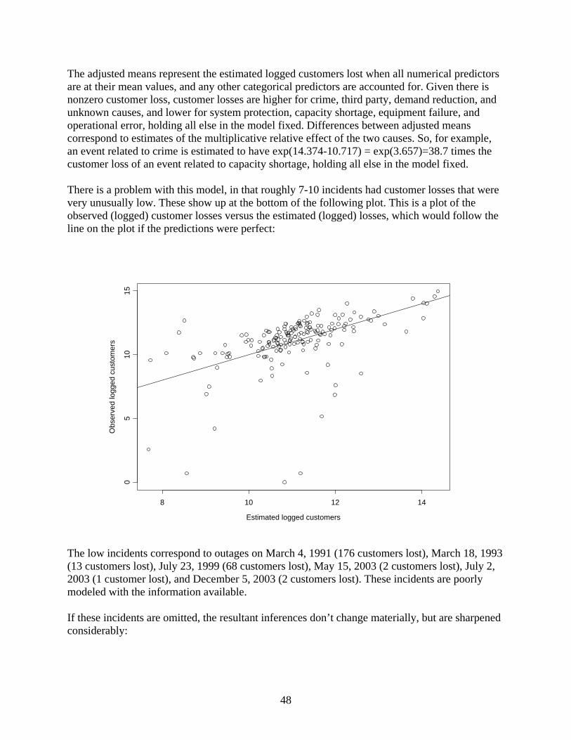
The adjusted means represent the estimated logged customers lost when all numerical predictors are at their mean values, and any other categorical predictors are accounted for. Given there is nonzero customer loss, customer losses are higher for crime, third party, demand reduction, and unknown causes, and lower for system protection, capacity shortage, equipment failure, and operational error, holding all else in the model fixed. Differences between adjusted means correspond to estimates of the multiplicative relative effect of the two causes. So, for example, an event related to crime is estimated to have exp(14.374-10.717) = exp(3.657)=38.7 times the customer loss of an event related to capacity shortage, holding all else in the model fixed. There is a problem with this model, in that roughly 7-10 incidents had customer losses that were very unusually low. These show up at the bottom of the following plot. This is a plot of the observed (logged) customer losses versus the estimated (logged) losses, which would follow the line on the plot if the predictions were perfect:

Estimated logged customers

Obs

erve

d lo

gged

cus

tom

ers

8 10 12 14

05

1015

The low incidents correspond to outages on March 4, 1991 (176 customers lost), March 18, 1993 (13 customers lost), July 23, 1999 (68 customers lost), May 15, 2003 (2 customers lost), July 2, 2003 (1 customer lost), and December 5, 2003 (2 customers lost). These incidents are poorly modeled with the information available. If these incidents are omitted, the resultant inferences don’t change materially, but are sharpened considerably:

49

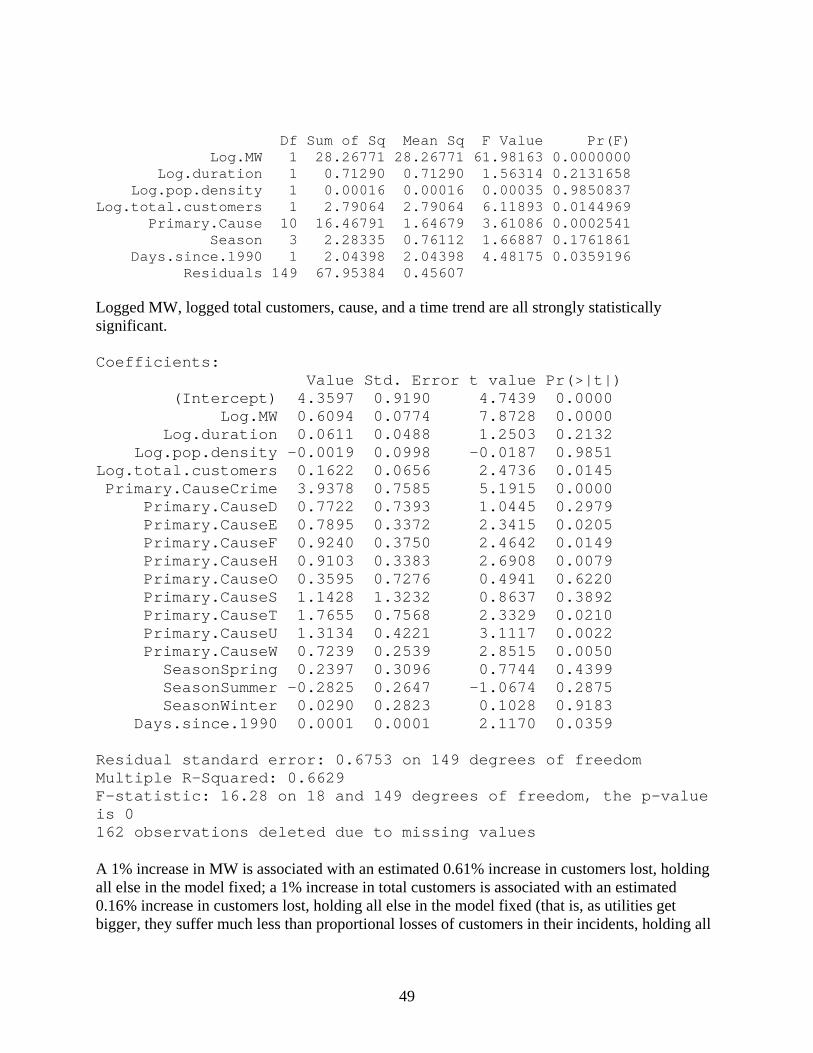
Df Sum of Sq Mean Sq F Value Pr(F) Log.MW 1 28.26771 28.26771 61.98163 0.0000000 Log.duration 1 0.71290 0.71290 1.56314 0.2131658 Log.pop.density 1 0.00016 0.00016 0.00035 0.9850837 Log.total.customers 1 2.79064 2.79064 6.11893 0.0144969 Primary.Cause 10 16.46791 1.64679 3.61086 0.0002541 Season 3 2.28335 0.76112 1.66887 0.1761861 Days.since.1990 1 2.04398 2.04398 4.48175 0.0359196 Residuals 149 67.95384 0.45607 Logged MW, logged total customers, cause, and a time trend are all strongly statistically significant. Coefficients: Value Std. Error t value Pr(>|t|) (Intercept) 4.3597 0.9190 4.7439 0.0000 Log.MW 0.6094 0.0774 7.8728 0.0000 Log.duration 0.0611 0.0488 1.2503 0.2132 Log.pop.density -0.0019 0.0998 -0.0187 0.9851 Log.total.customers 0.1622 0.0656 2.4736 0.0145 Primary.CauseCrime 3.9378 0.7585 5.1915 0.0000 Primary.CauseD 0.7722 0.7393 1.0445 0.2979 Primary.CauseE 0.7895 0.3372 2.3415 0.0205 Primary.CauseF 0.9240 0.3750 2.4642 0.0149 Primary.CauseH 0.9103 0.3383 2.6908 0.0079 Primary.CauseO 0.3595 0.7276 0.4941 0.6220 Primary.CauseS 1.1428 1.3232 0.8637 0.3892 Primary.CauseT 1.7655 0.7568 2.3329 0.0210 Primary.CauseU 1.3134 0.4221 3.1117 0.0022 Primary.CauseW 0.7239 0.2539 2.8515 0.0050 SeasonSpring 0.2397 0.3096 0.7744 0.4399 SeasonSummer -0.2825 0.2647 -1.0674 0.2875 SeasonWinter 0.0290 0.2823 0.1028 0.9183 Days.since.1990 0.0001 0.0001 2.1170 0.0359 Residual standard error: 0.6753 on 149 degrees of freedom Multiple R-Squared: 0.6629 F-statistic: 16.28 on 18 and 149 degrees of freedom, the p-value is 0 162 observations deleted due to missing values A 1% increase in MW is associated with an estimated 0.61% increase in customers lost, holding all else in the model fixed; a 1% increase in total customers is associated with an estimated 0.16% increase in customers lost, holding all else in the model fixed (that is, as utilities get bigger, they suffer much less than proportional losses of customers in their incidents, holding all

50

else fixed); each passing year is associated with an estimated 4.2% increase in customers lost given all else in the model is held fixed. The pattern related to causes is as follows: Primary.Cause C Crime D E F H O S 10.657 14.595 11.430 11.447 11.581 11.568 11.017 11.800 se 0.219 0.721 0.728 0.265 0.293 0.243 0.682 1.299 T U W 12.423 11.971 11.381 se 0.705 0.321 0.142 We see that given there is nonzero customer loss, customer losses are higher for crime, third party, and unknown causes, and lower for capacity shortage and operational error, holding all else in the model fixed. Predictions based on the model follow the observed values reasonably well, although there are still more unusually low values than unusually high values:


Obs

erve

d lo

gged

cus

tom

ers

9 10 11 12 13 14

810

1214

It is not clear that logged MW should be used as a predictor of logged customers lost, since one could argue that both are results of the inherent severity of the incident. This can be explored by refitting the regression models without the logged MW predictor. We start with an ordinary least squares model, but not surprisingly, this exhibits nonconstant variance. The weighted least squares model is as follows:

51

Df Sum of Sq Mean Sq F Value Pr(F) Log.duration 1 1.5852 1.585234 1.538035 0.2164727 Log.pop.density 1 1.1451 1.145137 1.111041 0.2932230 Log.total.customers 1 6.2401 6.240108 6.054314 0.0147849 Primary.Cause 11 54.6587 4.968974 4.821027 0.0000016 Season 3 0.4849 0.161617 0.156805 0.9251973 Days.since.1990 1 0.4341 0.434131 0.421205 0.5171368 Residuals 186 191.7080 1.030688 The only significant terms are those for logged total customers and primary cause. Here is a summary of the model: Coefficients: Value Std. Error t value Pr(>|t|) (Intercept) 5.7295 1.4848 3.8586 0.0002 Log.duration 0.0894 0.0721 1.2402 0.2165 Log.pop.density 0.1475 0.1399 1.0541 0.2932 Log.total.customers 0.2343 0.0952 2.4606 0.0148 Primary.CauseCrime 3.6588 1.1444 3.1970 0.0016 Primary.CauseD 1.3423 1.1239 1.1943 0.2339 Primary.CauseE 0.6946 0.4811 1.4439 0.1505 Primary.CauseF 1.4748 0.8339 1.7687 0.0786 Primary.CauseH 1.2778 0.5416 2.3592 0.0194 Primary.CauseN 5.3388 1.5278 3.4945 0.0006 Primary.CauseO 1.6409 1.0981 1.4943 0.1368 Primary.CauseS -0.1313 1.8096 -0.0726 0.9422 Primary.CauseT 3.2755 1.0816 3.0285 0.0028 Primary.CauseU 3.2880 0.6495 5.0622 0.0000 Primary.CauseW 1.4214 0.3548 4.0056 0.0001 SeasonSpring -0.2523 0.4379 -0.5762 0.5652 SeasonSummer -0.2459 0.3932 -0.6254 0.5325 SeasonWinter -0.2514 0.4172 -0.6027 0.5475 Days.since.1990 0.0001 0.0001 0.6490 0.5171 Residual standard error: 1.015 on 186 degrees of freedom Multiple R-Squared: 0.2663 F-statistic: 3.75 on 18 and 186 degrees of freedom, the p-value is 2.06e-006 A 1% increase in total customers is associated with a 0.23% estimated increase in customers lost, holding all else in the model fixed. The primary cause effect is summarized by the adjusted means:

52

Primary.Cause C Crime D E F H N O 9.932 13.590 11.274 10.626 11.406 11.209 15.270 11.572 se 0.320 1.073 1.076 0.365 0.768 0.420 1.498 1.049 S T U W 9.800 13.207 13.220 11.353 se 1.783 1.042 0.586 0.185 Customer losses are higher for natural disaster, crime, unknown causes, and third party, and lower for system protection, capacity shortage, and equipment failure, holding all else in the model fixed. This might be viewed as a more intuitive result than that in the earlier model, since the largest customer losses are coming from causes that are clearly beyond the control of the utility, while the smallest losses are coming from causes that are internal to the utility. The unusually small customer losses still show up as distinct:


Obs

erve

d lo

gged

cus

tom

ers

8 9 10 11 12 13 14

05

1015

If these incidents are omitted, logged duration now comes in as a significant predictor.

53

Df Sum of Sq Mean Sq F Value Pr(F) Log.duration 1 2.56276 2.562762 5.232056 0.0233378 Log.pop.density 1 0.77118 0.771181 1.574418 0.2111933 Log.total.customers 1 3.08369 3.083692 6.295570 0.0129871 Primary.Cause 11 50.31277 4.573888 9.337910 0.0000000 Season 3 2.10399 0.701330 1.431813 0.2350431 Days.since.1990 1 0.45808 0.458078 0.935199 0.3348132 Residuals 180 88.16747 0.489819 Coefficients: Value Std. Error t value Pr(>|t|) (Intercept) 6.4084 1.0787 5.9409 0.0000 Log.duration 0.1163 0.0508 2.2874 0.0233 Log.pop.density 0.1218 0.0970 1.2548 0.2112 Log.total.customers 0.1768 0.0705 2.5091 0.0130 Primary.CauseCrime 3.9623 0.7907 5.0113 0.0000 Primary.CauseD 1.0758 0.7762 1.3860 0.1675 Primary.CauseE 1.2282 0.3371 3.6429 0.0004 Primary.CauseF 1.5693 0.5756 2.7262 0.0070 Primary.CauseH 1.4230 0.3764 3.7803 0.0002 Primary.CauseN 4.7145 1.0940 4.3093 0.0000 Primary.CauseO 1.5332 0.7595 2.0189 0.0450 Primary.CauseS 1.5843 1.4367 1.1027 0.2716 Primary.CauseT 3.3238 0.7458 4.4568 0.0000 Primary.CauseU 3.3640 0.4484 7.5030 0.0000 Primary.CauseW 1.5631 0.2450 6.3804 0.0000 SeasonSpring 0.2893 0.3055 0.9467 0.3451 SeasonSummer -0.1906 0.2720 -0.7007 0.4844 SeasonWinter -0.1058 0.2883 -0.3672 0.7139 Days.since.1990 0.0001 0.0001 0.9671 0.3348 Residual standard error: 0.6999 on 180 degrees of freedom Multiple R-Squared: 0.4231 F-statistic: 7.335 on 18 and 180 degrees of freedom, the p-value is 5.751e-014 A 1% increase in duration is associated with an estimated 0.12% increase in customers lost, holding all else in the model fixed; a 1% increase in customers is associated with an estimated 0.18% increase in customers lost, holding all else in the model fixed. The primary cause effect is summarized below:

54

Primary.Cause C Crime D E F H N O 9.960 13.923 11.036 11.189 11.530 11.383 14.675 11.494 se 0.221 0.741 0.742 0.258 0.530 0.293 1.075 0.725 S T U W 11.545 13.284 13.324 11.524 se 1.421 0.718 0.405 0.128 Customer losses are higher for natural disaster, crime, unknown causes, and third party, and lower for capacity shortage, demand reduction, and equipment failure, holding all else in the model fixed. Although demand reduction has replaced system protection as being associated with low customer losses when the smallest losses are omitted, the pattern still remains: the largest customer losses are coming from causes that are clearly beyond the control of the utility, while the smallest losses are coming from causes that are internal to the utility. B. Analysis of duration at the event level This section examines regression modeling for the (logged) duration of each incident. As was noted earlier, this allows for event-level characteristics to be used as predictors, but is based on a response variable that is much more variable than in the three-, six-, and twelve-month average analyses summarized earlier. First, here are plots of the observed relationships.

55

Logged total customers

Logg

ed d

urat

ion

5 10 15

-4-2

02

46

Logged population density

Logg

ed d

urat

ion

0 2 4 6 8

-4-2

02

46

Days since 1990

Logg

ed d

urat

ion

0 1000 2000 3000 4000 5000

-4-2

02

46

-4-2

02

46

Autumn Spring Summer Winter

Season

Logg

ed d

urat

ion

56

-4-2

02

46


Primary cause

Logg

ed d

urat

ion

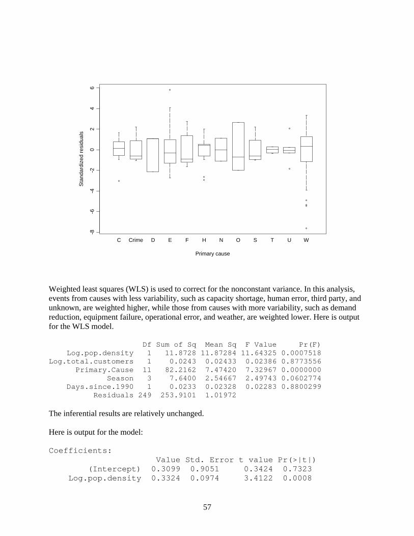
We see that there is little evidence of a relationship between logged duration and logged total customers. There is evidence of a positive relationship with logged population density (ignoring the two rare events at the very high population density level). There is weak evidence of the time trend on duration (note that since this plot is in the logged scale, trends upwards will be less apparent than in the original scale). There is some evidence of a season effect, with winter and spring events longer and autumn and summer events shorter. There is a clear relationship with primary cause. Note in particular that the two most common causes, equipment failure and weather are very different, with the former associated with shorter events and the latter associated with longer ones. A least squares regression implies that logged population density, primary cause, and season are significant predictors, but there is extreme nonconstant variance related to primary cause. Df Sum of Sq Mean Sq F Value Pr(F) Log.pop.density 1 15.7092 15.70916 5.043797 0.0255918 Log.total.customers 1 0.1415 0.14149 0.045427 0.8313946 Primary.Cause 11 202.8429 18.44027 5.920681 0.0000000 Season 3 24.3224 8.10748 2.603098 0.0525254 Days.since.1990 1 2.2344 2.23440 0.717407 0.3978090 Residuals 249 775.5232 3.11455 Here are side-by-side boxplots of the residuals separated by cause, which illustrates the nonconstant variance.

57

-8-6

-4-2

02

46


Primary cause

Sta

ndar

dize

d re

sidu

als

Weighted least squares (WLS) is used to correct for the nonconstant variance. In this analysis, events from causes with less variability, such as capacity shortage, human error, third party, and unknown, are weighted higher, while those from causes with more variability, such as demand reduction, equipment failure, operational error, and weather, are weighted lower. Here is output for the WLS model. Df Sum of Sq Mean Sq F Value Pr(F) Log.pop.density 1 11.8728 11.87284 11.64325 0.0007518 Log.total.customers 1 0.0243 0.02433 0.02386 0.8773556 Primary.Cause 11 82.2162 7.47420 7.32967 0.0000000 Season 3 7.6400 2.54667 2.49743 0.0602774 Days.since.1990 1 0.0233 0.02328 0.02283 0.8800299 Residuals 249 253.9101 1.01972 The inferential results are relatively unchanged. Here is output for the model: Coefficients: Value Std. Error t value Pr(>|t|) (Intercept) 0.3099 0.9051 0.3424 0.7323 Log.pop.density 0.3324 0.0974 3.4122 0.0008

58

Log.total.customers 0.0078 0.0504 0.1545 0.8774 Primary.CauseCrime 0.0212 0.8518 0.0249 0.9801 Primary.CauseD -1.1692 1.1500 -1.0167 0.3103 Primary.CauseE -0.6795 0.4078 -1.6662 0.0969 Primary.CauseF -0.2449 0.6356 -0.3854 0.7003 Primary.CauseH -2.2477 0.5341 -4.2085 0.0000 Primary.CauseN -1.6121 1.2369 -1.3033 0.1937 Primary.CauseO -0.5587 1.4469 -0.3861 0.6998 Primary.CauseS 0.2674 0.8710 0.3070 0.7591 Primary.CauseT 0.4361 0.4262 1.0232 0.3072 Primary.CauseU 1.7313 0.6414 2.6993 0.0074 Primary.CauseW 0.9379 0.3760 2.4945 0.0133 SeasonSpring 0.0507 0.3721 0.1362 0.8918 SeasonSummer -0.3310 0.3323 -0.9959 0.3203 SeasonWinter 0.4791 0.3673 1.3043 0.1933 Days.since.1990 0.0000 0.0001 0.1511 0.8800 Residual standard error: 1.01 on 249 degrees of freedom Multiple R-Squared: 0.3218 F-statistic: 6.949 on 17 and 249 degrees of freedom, the p-value is 1.111e-013 133 observations deleted due to missing values The model implies that a 1% increase in population density is associated with a 0.33% increase in duration, holding all else in the model fixed. The primary cause and season effects are summarized by the adjusted means: Primary.Cause C Crime D E F H N 2.1383 2.1595 0.9691 1.4588 1.8934 -0.1094 0.5262 se 0.3410 0.7777 1.1014 0.2056 0.5381 0.3960 1.1786 O S T U W 1.5796 2.4057 2.5744 3.8696 3.0762 se 1.4105 0.7945 0.2536 0.5452 0.1789 Season Autumn Spring Summer Winter 1.8288 1.8794 1.4978 2.3078 se 0.3478 0.3106 0.2460 0.2919 The season effect is noting that, holding all else in the model fixed, winter events have expected duration that is 2.25 times the duration of summer events, with autumn and spring in between. Presumably this has something to do with issues like the difficulty in traveling to downed power lines in snow and ice.

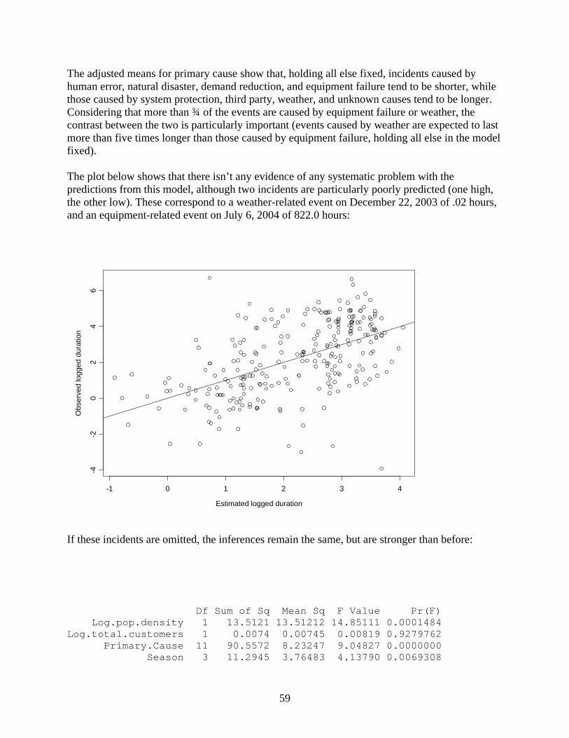
59

The adjusted means for primary cause show that, holding all else fixed, incidents caused by human error, natural disaster, demand reduction, and equipment failure tend to be shorter, while those caused by system protection, third party, weather, and unknown causes tend to be longer. Considering that more than ¾ of the events are caused by equipment failure or weather, the contrast between the two is particularly important (events caused by weather are expected to last more than five times longer than those caused by equipment failure, holding all else in the model fixed). The plot below shows that there isn’t any evidence of any systematic problem with the predictions from this model, although two incidents are particularly poorly predicted (one high, the other low). These correspond to a weather-related event on December 22, 2003 of .02 hours, and an equipment-related event on July 6, 2004 of 822.0 hours:

Estimated logged duration

Obs

erve

d lo

gged

dur

atio

n

-1 0 1 2 3 4

-4-2

02

46

If these incidents are omitted, the inferences remain the same, but are stronger than before: Df Sum of Sq Mean Sq F Value Pr(F) Log.pop.density 1 13.5121 13.51212 14.85111 0.0001484 Log.total.customers 1 0.0074 0.00745 0.00819 0.9279762 Primary.Cause 11 90.5572 8.23247 9.04827 0.0000000 Season 3 11.2945 3.76483 4.13790 0.0069308

60

Days.since.1990 1 0.0036 0.00364 0.00400 0.9496319 Residuals 247 224.7303 0.90984 Here is a summary of the model: Coefficients: Value Std. Error t value Pr(>|t|) (Intercept) 0.2569 0.8564 0.3000 0.7644 Log.pop.density 0.3557 0.0923 3.8537 0.0001 Log.total.customers 0.0043 0.0477 0.0905 0.9280 Primary.CauseCrime -0.0280 0.8048 -0.0348 0.9723 Primary.CauseD -1.1358 1.0865 -1.0454 0.2969 Primary.CauseE -0.7180 0.3863 -1.8585 0.0643 Primary.CauseF -0.1610 0.6006 -0.2681 0.7888 Primary.CauseH -2.2390 0.5048 -4.4355 0.0000 Primary.CauseN -1.7305 1.1688 -1.4806 0.1400 Primary.CauseO -0.5046 1.3668 -0.3692 0.7123 Primary.CauseS 0.3997 0.8231 0.4855 0.6277 Primary.CauseT 0.5454 0.4031 1.3532 0.1772 Primary.CauseU 1.8346 0.6061 3.0268 0.0027 Primary.CauseW 1.0477 0.3561 2.9424 0.0036 SeasonSpring 0.0403 0.3515 0.1148 0.9087 SeasonSummer -0.4000 0.3144 -1.2724 0.2044 SeasonWinter 0.5937 0.3480 1.7062 0.0892 Days.since.1990 0.0000 0.0001 -0.0632 0.9496 Residual standard error: 0.9539 on 247 degrees of freedom Multiple R-Squared: 0.3705 F-statistic: 8.55 on 17 and 247 degrees of freedom, the p-value is 0 133 observations deleted due to missing values A 1% increase in population density is associated with an estimated 0.36% increase in customers lost, holding all else in the model fixed. The patterns related to causes and seasons are as follows: Primary.Cause C Crime D E F H N 2.1135 2.0854 0.9776 1.3954 1.9524 -0.1255 0.3829 se 0.3225 0.7346 1.0403 0.1952 0.5084 0.3739 1.1135 O S T U W 1.6088 2.5131 2.6589 3.9481 3.1611 se 1.3324 0.7508 0.2401 0.5152 0.1699

61

Season Autumn Spring Summer Winter 1.8308 1.8711 1.4308 2.4245 se 0.3285 0.2933 0.2327 0.2767 The season effect implies that, holding all else in the model fixed, winter events have expected duration that is 2.7 times the duration of summer events, with autumn and spring events in the middle. The adjusted means for primary cause show that, holding all else fixed, incidents caused by human error, natural disaster, demand reduction, and equipment failure tend to be shorter, while those caused by system protection, third party, weather, and unknown causes tend to be longer. In particular, events caused by weather are expected to last almost six times longer than those caused by equipment failure, holding all else fixed. The model tracks the observed logged durations reasonably well.

Estimated logged duration

Obs

erve

d lo

gged

dur

atio

n

-1 0 1 2 3 4

-20

24

6

The absence of a time trend in this model, given the earlier evidence for one in the season-level analysis, is worth comment. An analysis just on the time trend (Days since 1990) does yield statistical significance, as the following output shows:

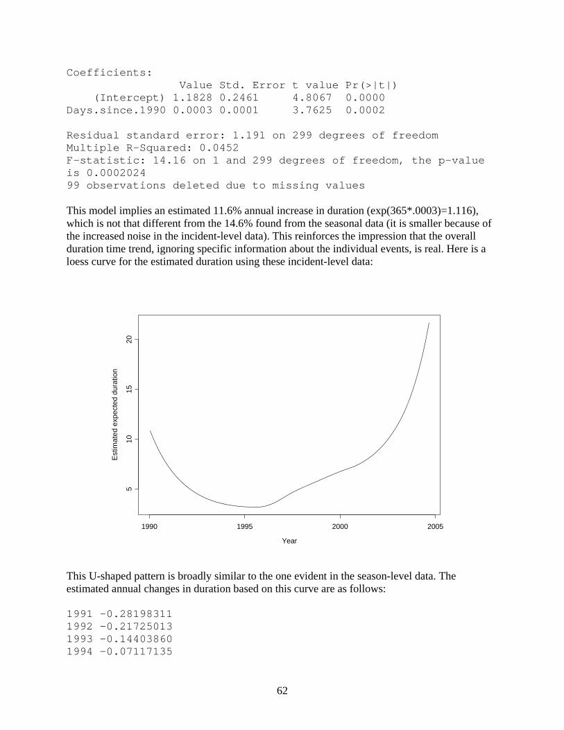
62

Coefficients: Value Std. Error t value Pr(>|t|) (Intercept) 1.1828 0.2461 4.8067 0.0000 Days.since.1990 0.0003 0.0001 3.7625 0.0002 Residual standard error: 1.191 on 299 degrees of freedom Multiple R-Squared: 0.0452 F-statistic: 14.16 on 1 and 299 degrees of freedom, the p-value is 0.0002024 99 observations deleted due to missing values This model implies an estimated 11.6% annual increase in duration (exp(365*.0003)=1.116), which is not that different from the 14.6% found from the seasonal data (it is smaller because of the increased noise in the incident-level data). This reinforces the impression that the overall duration time trend, ignoring specific information about the individual events, is real. Here is a loess curve for the estimated duration using these incident-level data:

Year

Est

imat

ed e

xpec

ted

dura

tion

1990 1995 2000 2005

510

1520

This U-shaped pattern is broadly similar to the one evident in the season-level data. The estimated annual changes in duration based on this curve are as follows: 1991 -0.28198311 1992 -0.21725013 1993 -0.14403860 1994 -0.07117135

63

1995 0.01160909 1996 0.25814792 1997 0.24967458 1998 0.16656962 1999 0.13245628 2000 0.11124667 2001 0.18375624 2002 0.28224436 2003 0.40632285 These can be compared to the season-level numbers from Section I. C., and they are very similar (a bit smaller, which reflects the additional noise in the event-level data). Up until 1994, durations were getting shorter. This turned around in 1995, and for a few years the average duration went up 15-25% annually. This was followed by a long period (1998-2001) of fairly stable growth of 10-20%. Finally, from 2002 on, average durations have started increasing again at a high 30-40% rate. Thus, the constant estimate of 11.6% annually obtained from the regression model actually seems to mask some very different periods in average duration change. There is another factor at play here that leads to the time trend disappearing in the regression model. The models in this section take into account the other potential predictors. Note the results of a model that adds season and logged population density to the time trend: Df Sum of Sq Mean Sq F Value Pr(F) Days.since.1990 1 7.1460 7.14605 5.527602 0.0194659 Season 3 2.1804 0.72681 0.562200 0.6404119 Log.pop.density 1 10.1482 10.14815 7.849787 0.0054649 Log.total.customers 1 3.5317 3.53168 2.731823 0.0995739 Residuals 260 336.1263 1.29279 The time variable is still highly significant, even with these other predictors. However, when primary cause is added, its significance disappears (as in the table earlier in this section), which shows that it is the primary cause effect that is driving the apparent time trend effect. (Note also that including primary cause allows a seasonal effect to show up, and the logged customers effect to disappear.) Recall that more than ¾ of the incidents are either equipment failure- or weather-related, and that incidents caused by equipment failure tend to be shorter, while weather-related ones tend to be longer. In fact, weather-related incidents are becoming more common, while equipment failure-related ones are becoming less common, and this accounts for much of the overall pattern of increasing average durations by season. The following plots show the changing proportions of incidents from these two causes at the semiannual level; it is clear that since the mid 1990s, relatively speaking equipment failures are going down and weather incidents are going up, while before that the opposite pattern was occurring. This corresponds exactly to the drop in durations up to 1995, and the increase since then noted earlier. Thus, it would seem that further study of why equipment failures are becoming less common (relatively speaking) and weather-related events are becoming more common is warranted.

64

Equipment failure

Year

Pro

porti

on o

f inc

iden

ts

1990 1992 1994 1996 1998 2000 2002 2004

0.0

0.2

0.4

0.6

0.8

1.0

Weather

Year

Pro

porti

on o

f inc

iden

ts

1990 1992 1994 1996 1998 2000 2002 2004

0.0

0.2

0.4

0.6

0.8

1.0

C. Using the models for scenario prediction These models provide useful information about the factors related to the seriousness of a power outage, but they also can be used to construct predictions for outage outcomes based on different scenarios. By examining predicted duration and customer loss under different conditions, it is possible to map out possible outage outcomes in the event of a terrorist attack (for which there is virtually no data). We look at scenarios for four different cities: New York, Chicago, San Francisco, and Seattle. Using the characteristics of the utilities in these four cities, the estimated duration of an incident, separated by season and cause, can be determined for each city using the weighted least squares model described on pages 53-54. Since (logged) duration is an important predictor for customer loss, these estimated durations can then be used as inputs to the logistic regression model discussed on pages 38-39 to estimate the probability that there is zero customer loss. Finally, the estimated (logged) duration value, along with the characteristics of the utility, are used to estimate the number of customers lost, given there is nonzero customer loss, using the weighted least squares model of pages 42-43. The estimated values for the four cities are given in the Appendix, along with overall estimated customer losses for several scenarios. In addition to estimated expected values, we can construct 50% prediction intervals for duration and for customer loss (given that the loss is nonzero) for any cause and season for the four cities. These intervals give the central range within which there is 50% chance of the duration or customer loss falling in an individual incident.

65

It is important to note that these predictions and prediction intervals are based on using city-specific values as inputs to models based on national data, rather than models tailored to each specific city. Thus, these results are best viewed as scenarios for cities with the general demographic characteristics of New York, Chicago, and so on, rather than as scenarios based on characteristics unique to each city. 1. Duration of an incident First, consider intervals for duration. The following figure gives 50% prediction intervals for duration of an incident in New York City during the summer.

C Crime D E F H N O S T U WPrimary cause

0

20

40

60

80

100

Dur

atio

n

50% prediction intervals for NYC summer outages

The horizontal tick on each line is the estimated expected duration for a summer New York City outage with that cause, while the vertical line gives the 50% prediction interval. The figure shows that the cause of the incident is related to both the level of duration (e.g., human error and demand reduction associated with shorter incidents and weather and unknown cause associated with longer ones) and the variability in duration (third party cause and system protection have similar expected durations, but durations of incidents caused by system protection are much more variable).

66

The following plot gives intervals for New York City outages during the winter.


0

50

100

150

200

250

Dur

atio

n

50% prediction intervals for NYC winter outages

The pattern of relative estimates and prediction intervals is the same as for the summer incidents, but the averages and intervals are shifted up by a factor of two, reflecting that outages are longer on average during the winter. The pattern of the intervals for a Chicago summer outage is again similar to that of the New York ones (as it must be), except that the intervals are shifted downwards, reflecting that the population density and number of customers serviced in Chicago imply a shorter expected duration of an incident.

67


0

20

40

60

80

Dur

atio

n50% prediction intervals for Chicago summer outages

The intervals for San Francisco are similar to those for Chicago, while those for Seattle are centered at somewhat lower values.

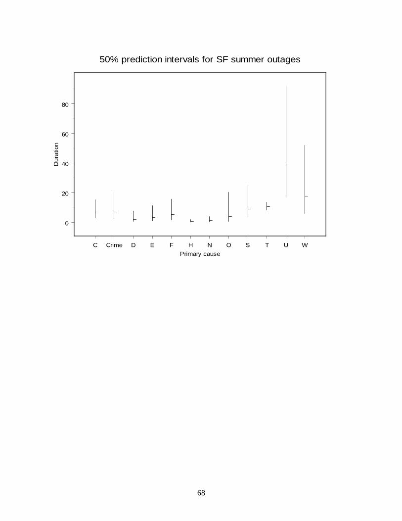
68


0

20

40

60

80

Dur

atio

n50% prediction intervals for SF summer outages

69


0

20

40

60

Dur

atio

n50% prediction intervals for Seattle summer outages

2. Customer loss of an incident, given that it is nonzero Using the estimated durations as inputs for the model, prediction intervals for customer loss (given that the loss is nonzero) also can be constructed. First, here are intervals for a summer outage in New York City.

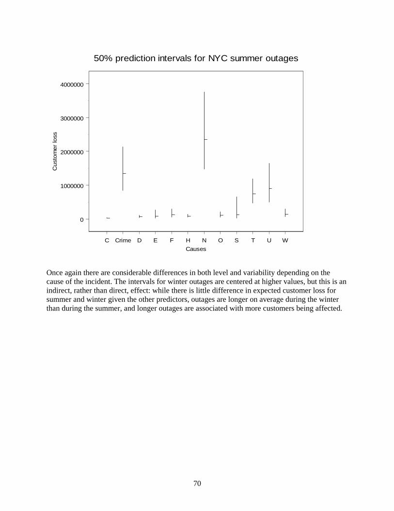
70

C Crime D E F H N O S T U WCauses

0

1000000

2000000

3000000

4000000

Cus

tom

er lo

ss50% prediction intervals for NYC summer outages

Once again there are considerable differences in both level and variability depending on the cause of the incident. The intervals for winter outages are centered at higher values, but this is an indirect, rather than direct, effect: while there is little difference in expected customer loss for summer and winter given the other predictors, outages are longer on average during the winter than during the summer, and longer outages are associated with more customers being affected.

71


0

1000000

2000000

3000000

4000000

Cus

tom

er lo

ss50% prediction intervals for NYC winter outages

Customer losses in Chicago and San Francisco are expected to be similar to those in New York, while those in Seattle have smaller losses (these patterns are being driven in large part by the number of customers that utilities in those cities serve).

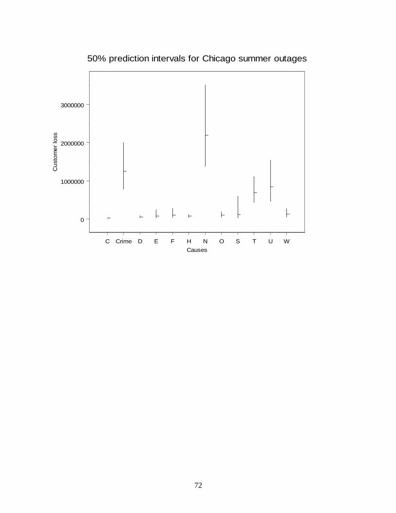
72


0

1000000

2000000

3000000

Cus

tom

er lo

ss50% prediction intervals for Chicago summer outages

73


0

1000000

2000000

3000000

4000000

Cus

tom

er lo

ss50% prediction intervals for SF summer outages

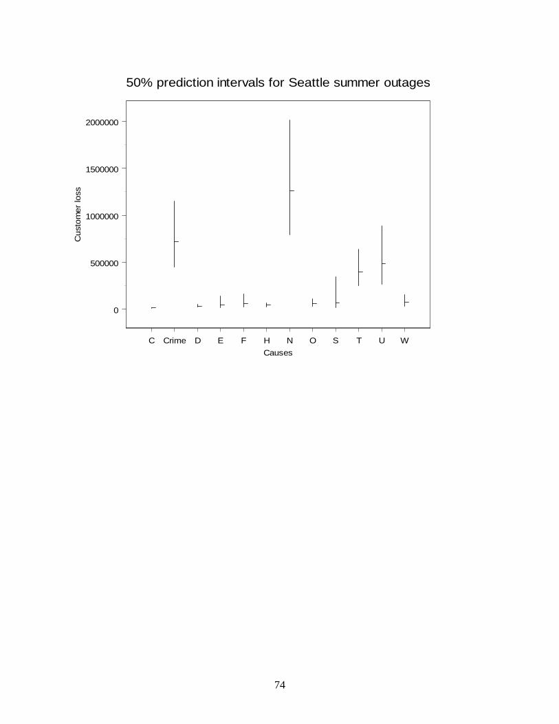
74


0

500000

1000000

1500000

2000000

Cus

tom

er lo

ss50% prediction intervals for Seattle summer outages

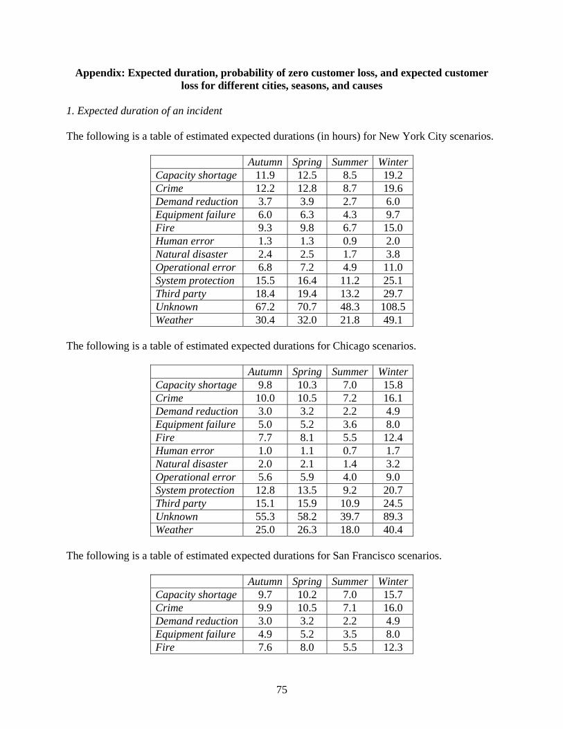
75

Appendix: Expected duration, probability of zero customer loss, and expected customer loss for different cities, seasons, and causes

1. Expected duration of an incident The following is a table of estimated expected durations (in hours) for New York City scenarios.

Autumn Spring Summer Winter Capacity shortage 11.9 12.5 8.5 19.2 Crime 12.2 12.8 8.7 19.6 Demand reduction 3.7 3.9 2.7 6.0 Equipment failure 6.0 6.3 4.3 9.7 Fire 9.3 9.8 6.7 15.0 Human error 1.3 1.3 0.9 2.0 Natural disaster 2.4 2.5 1.7 3.8 Operational error 6.8 7.2 4.9 11.0 System protection 15.5 16.4 11.2 25.1 Third party 18.4 19.4 13.2 29.7 Unknown 67.2 70.7 48.3 108.5 Weather 30.4 32.0 21.8 49.1

The following is a table of estimated expected durations for Chicago scenarios.


The following is a table of estimated expected durations for San Francisco scenarios.

Autumn Spring Summer Winter Capacity shortage 9.7 10.2 7.0 15.7 Crime 9.9 10.5 7.1 16.0 Demand reduction 3.0 3.2 2.2 4.9 Equipment failure 4.9 5.2 3.5 8.0 Fire 7.6 8.0 5.5 12.3

76

Human error 1.0 1.1 0.7 1.7 Natural disaster 1.9 2.0 1.4 3.1 Operational error 5.6 5.9 4.0 9.0 System protection 12.7 13.4 9.1 20.5 Third party 15.0 15.8 10.8 24.3 Unknown 54.9 57.8 39.5 88.7 Weather 24.8 26.1 17.8 40.1

The following is a table of estimated expected durations for Seattle scenarios.


2. Probability of zero customer loss The following is a table of estimated probabilities that an incident will have zero customer loss for New York City scenarios.

Autumn Spring Summer Winter Capacity shortage .049 .056 .028 .052 Crime .431 .464 .300 .447 Demand reduction .542 .575 .401 .558 Equipment failure .047 .053 .027 .050 Fire .047 .054 .027 .050 Human error .059 .066 .034 .0622 Natural disaster .117 .132 .070 .124 Operational error .019 .022 .011 .020 System protection .000 .000 .000 .000 Third party .485 .519 .348 .502 Unknown .034 .039 .019 .036 Weather .007 .008 .004 .007

77

The following is a table of estimated probabilities that an incident will have zero customer loss for Chicago scenarios.


The following is a table of estimated probabilities that an incident will have zero customer loss for San Francisco scenarios.


The following is a table of estimated probabilities that an incident will have zero customer loss for Seattle scenarios.

Autumn Spring Summer Winter Capacity shortage .131 .148 .079 .139 Crime .689 .718 .557 .703 Demand reduction .776 .799 .663 .787 Equipment failure .125 .141 .075 .132 Fire .127 .143 .076 .134 Human error .154 .172 .093 .163 Natural disaster .280 .308 .180 .293

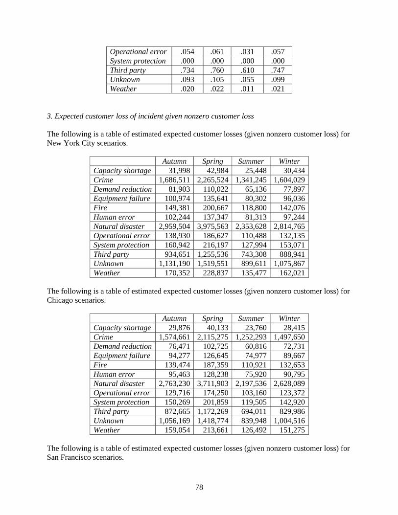
78

Operational error .054 .061 .031 .057 System protection .000 .000 .000 .000 Third party .734 .760 .610 .747 Unknown .093 .105 .055 .099 Weather .020 .022 .011 .021

3. Expected customer loss of incident given nonzero customer loss The following is a table of estimated expected customer losses (given nonzero customer loss) for New York City scenarios.

Autumn Spring Summer Winter Capacity shortage 31,998 42,984 25,448 30,434 Crime 1,686,511 2,265,524 1,341,245 1,604,029 Demand reduction 81,903 110,022 65,136 77,897 Equipment failure 100,974 135,641 80,302 96,036 Fire 149,381 200,667 118,800 142,076 Human error 102,244 137,347 81,313 97,244 Natural disaster 2,959,504 3,975,563 2,353,628 2,814,765 Operational error 138,930 186,627 110,488 132,135 System protection 160,942 216,197 127,994 153,071 Third party 934,651 1,255,536 743,308 888,941 Unknown 1,131,190 1,519,551 899,611 1,075,867 Weather 170,352 228,837 135,477 162,021

The following is a table of estimated expected customer losses (given nonzero customer loss) for Chicago scenarios.


The following is a table of estimated expected customer losses (given nonzero customer loss) for San Francisco scenarios.

79


The following is a table of estimated expected customer losses (given nonzero customer loss) for Seattle scenarios.

Autumn Spring Summer Winter Capacity shortage 17,144 23,030 13,634 16,305 Crime 903,585 1,213,804 718,601 859,394 Demand reduction 43,881 58,947 34,898 41,735 Equipment failure 54,099 72,672 43,024 51,453 Fire 80,034 107,512 63,650 76,120 Human error 54,780 73,587 43,565 52,101 Natural disaster 1,585,619 2,129,995 1,261,008 1,508,072 Operational error 74,435 99,990 59,196 70,794 System protection 86,228 115,832 68,576 82,011 Third party 500,760 672,681 398,243 476,269 Unknown 606,060 814,133 481,986 576,419 Weather 91,270 122,605 72,585 86,806

These estimates can be combined to estimate the overall (unconditional) expected number of customers lost for a given scenario. If p is the probability of zero customer loss, the expected number of customers lost is

E(Customers lost) = (p)(0) + (1-p)(E[Customers lost given nonzero customer loss]) So, for example, since an incident in New York City during the winter caused by crime has zero customer loss with probability p=.447 and nonzero loss with probability 1-p=.553, and an expected 1,604,029 customers lost if there is nonzero loss, the overall expected customers lost for such an incident is

E(Customers lost) = (.447)(0) + (.553)(1,604,029) = 887,028.

80

References

1. Simonoff, J.S. (1996), Smoothing Methods in Statistics, Springer-Verlag, New York. 2. Simonoff, J.S. (2003), Analyzing Categorical Data, Springer-Verlag, New York.

electricity case: statistical analysis of electric power...

Documents