1

Electromagnetic Compatibility for Space Structure Design

E3 numerical assessment in aeronautics

Miguel R. Cabello1, Sergio Fernandez2, Marc Pous3, Enrique Pascual-Gil4, Luis D. Angulo1, David Poyatos2, Mireya Fernandez3, Guadalupe G. Gutierrez4,

Amelia R. Bretones1, Manuel Añón2, Ferran Silva3, Jesus Alvarez4, Mario F. Pantoja1, Borja Plaza5, Luis Nuño6,

Rafael G. Martin1, David Escot2, Pere J. Riu3, Rafael Trallero2, Ricardo Jaúregui3, Salvador G. Garcia1

1University of Granada (UGR), Spain 2National Institute of Aerospace Technology (INTA), Spain

3Universitat Politècnica de Catalunya (UPC), Spain 4AIRBUS, Spain

5Ingeniería de Sistemas para la Defensa de España S.A. (ISDEFE), Spain 6Polytechnic University of Valencia (UPV), Spain

INTRODUCTION & BACKGROUND

Modern aircrafts have become increasingly dependent on electronic equipment to control its systems. This has led to new safety concerns with respect to their immunity levels against EM hazards and, in consequence, their assessment by aircraft manufacturers. Besides, the variety of potential EMI sources are increasing dramatically due to the appearing of new artificial sources in addition to the natural ones. This situation is aggravated by the pervasive use of composite materials in aircraft structure: CFC, CFRC, CFRP, etc. These materials, lighter and stronger from the mechanical point of view, are poorer conductors than metals and therefore have lower shielding capabilities. From the EMC point of view, the main EM threats for an AV can be summarized as follows:

• Lightning Indirect Effects (LIE): 0 to ~50 MHz. Indirect effects are caused by the electric current flowing through the structure and internal wiring as a consequence of the impact of a lightning strike. This is, undoubtedly, the most important threat to onboard electronic equipment, becoming critical for aircrafts mostly made of CFCs (Meyer et al., 2008) like, for instance, modern UAVs.

• High Intensity Radiated Fields (HIRF): 0 to ~100 MHz. This threat is caused by artificial intentional or unintentional, external or internal RF sources. These are constantly increasing in number: TV, mobile networks (3G/4G/5G), radars, navigation satellite systems, etc. and may couple to cables and equipment, potentially causing malfunction for high field levels.

2

• Electromagnetic Pulses (EMP) of nuclear or non-nuclear origin: 0-100 MHz. Most of current non-nuclear low-level electromagnetic pulse generators are not capable of radiating enough EM energy to produce a significant damage. However, novel devices are appearing, which are able to involve much higher power levels with extremely short durations. These modern weapons, also named E-bombs, are becoming cheaper and susceptible of being used in terrorist acts. They can wreak havoc on computers and networks, yielding temporary disruptive effects (Radasky et al., 2004; Radasky, 2014).

In all these cases, as a result of the exposition to the EM hazard, transient currents will flow along the aircraft surface, creating EM fields which penetrate into the fuselage through apertures such as windows, or by diffusion through parts made of poorly conducting materials (Figure 1). Inside the aircraft, these transients induce currents to the EWIS, which, in turn, couple to equipment, potentially compromising their safe operation or even creating permanent damage. Several aviation incidents, reported in the last quarter of the past century, triggered the attention of aviation agencies to include strict EMC requirements for the airworthiness certification processes of AVs during their whole life-cycle. Before a newly developed AV model is permitted to operate, it must get a certificate of airworthiness issued by an aviation regulatory authority. For instance, in civil aviation, the regulatory authority is the EASA in the EU, or the FAA in the US. Within the EMC context, certification methods are mainly based on experimental tests and the guidelines provided in several standardized documents and certification guides: Eurocae ED-105/SAE-ARP5416; SAE-ARP5415; Eurocae ED-107/SAE-ARP5583; MIL-STD-202; MIL-STD-461;EUROCAE ED-14/RTCA/DO-160, MIL-STD-464, STANAG 4370, etc..

Figure 1: Typical EM Hazard in aeronautics. Reprinted from (Cabello, 2017d). Classically, the EMC assessment of EMI in the aeronautic industry has relied on experimental campaigns, often carried out at late stages of the aircraft manufacturing when correction and redesign costs due to unforeseen EMI issues are prohibitive. Nowadays, the computing power of modern clusters is making it possible to employ CEM tools to simulate and predict EMC issues. At early stages of design, these allow engineers to make design decisions like the use of alternative cable routings, shielding materials, bonding components, material replacement, return network addition, etc. CEM tools are demonstrating their utility

3

at all the design phases of an aircraft, to improve EMC safety aspects, and to ease and speed up the experimental certification process. However, international aviation agencies are still reluctant to accept simulations as a replacement of experimental tests. To achieve this, strict procedures need to be consolidated, and standard engineering guidelines must be agreed. These must describe a systematic methodology to achieve validated computational models, suitable to produce data which is acceptable for certification purposes. A formal declaration about this topic was stated by the EASA and constituted one of the main outcomes of the HIRF-SE project, funded by the European Union under the FP7 program between 2008 and 2013, with a 23 M€ budget. This project gathered over 40 partners from 11 EU countries, including all major universities, airframers, test-houses, and software-houses. The main target was to build a synthetic framework to be used for the validation of numerical solvers with experimental data in the assessment of HIRF effects on AVs. During HIRF-SE, the concept of a validated model for a specific AV was settled down. Such a model must include, with full traceability and reproducibility, the whole path necessary to achieve the input required by the computer solver; starting from the CAD data of the AV and the experimental setup, with the steps followed to clean, simplify, and mesh it, resulting in the actual input file fed to the solver. It must also include all the mathematical models (material treatment, cables, sources, post-processing…) used by the solver, the methods employed for its computer implementation, the executable version of all the tools used in the process, and the solver itself used for the simulation. Finally, a sufficient set of experimental and simulation data agreeing according to some consolidated validation criterion must also be provided. The typical workflow of the whole procedure is given in Figure 2.

Figure 2: CEM for EMC workflow in aeronautics. Several other European partners, including all major aeronautic stakeholders, agencies and public research entities, have also pointed in the same direction1. Some of these comments have been included in the EUROCAE certification guides for numerical methods (Eurocae ED-107A, 2010), as a support for experimental campaigns. At Spanish national level, the HIRF-SE project was continued through several other projects (UAVEMI, UAVE3, Alhambra-UGRFDTD…) funded by the Ministry of Economy, the Andalusian regional govt., and by AIRBUS. These projects gather a military national airworthiness agency (INTA), a major airframer (AIRBUS), and three top-ranked universities (UGR, UPC and UPV). A representative set of researchers of these institutions are co-authors of this work, responsible for measurement campaigns, CAD treatment, simulations, validations, etc. Among other achievements, these projects have served to build and validate2 the SEMBA-UGRFDTD solver (Garcia et al., 2013), used for the simulations presented in this chapter. This solver is capable of treating the complexity found in EMC test-setups and its maturity has been achieved after broad validations, which include cross-comparisons with commercial

1 Some projects on this line are: FULMEN, ILDAS, EM-HAZ, STRUCTURES, GENIAL, ARROW, SAFETEL, GEMCAR, SARITSU, FLAVIIR, MOVEA, etc. 2 See http://cordis.europa.eu/result/rcn/140447_en.html

4

and in-house time and frequency-domain solvers, and with experimental data (Gutierrez et al., 2012; Gil & Gutierrez, 2011). The main objectives of this chapter are to provide stones that pave the way for such a roadmap. It is divided in two parts. In the first one, the authors revisit some of the most common procedures employed in E3 certification in aeronautics. Next, a short description of the basic FDTD method is given. References of the required extensions and models of the basic method to cope with the complexity found in certification setups are also pointed out, paying special attention to the material and cable modeling. The guidelines to build computationally affordable models, retaining all the relevant physics that are present in the experimental setup are also described and put in relation to CAD geometrical cleaning, simplification and meshing. The FSV standard (IEEE Std 1597.1, 2008) is also presented as a tool for an automatic validation procedure to assess the matching between experimental and numerical results. Such expert-like tools are definitely required in this complex discipline where the incertitude in parameters is often not well controlled. The second part of the chapter provides application examples of the procedures discussed in the first part. Three examples of experimental EMC certification scenarios are described: a radiated test-setup for the AIRBUS C-295 aircraft, a reverberating chamber setup for the central fuselage of the INTA MILANO UAV, both for HIRF analysis; and a conducted current setup for the INTA SIVA UAV for LIE assessment. Most of the experiences described here in the context of aircraft EMC analysis, can be fully extended to general space systems, which are also susceptible to some of the threats described above, apart from some other ones intrinsically due to being without the protection of the earth atmosphere and magnetosphere. TESTS FOR AERONAUTICAL E3 COMPLIANCE Let us now revisit three common test setups for aircrafts, considered in the (Eurocae ED-107A, 2010) and (Eurocae ED-105A, 2013) aircraft certification guides3:

1. Direct Drive (DD) (or Direct Current Injection (DCI)) tests. The aim of this test is to find the current which couples to the internal cables of the aircraft when a current is injected and drained on different points of the fuselage (Figure 3). The combination of injection and drain points must be such that it represents the worst cases of operation. To this end, the standard recommends the design and construction of a coaxial return wire network around the aircraft to minimize the radiation to the exterior (Eurocae ED-107A, 2010). This configuration maximizes the ratio between induced currents and source power and extends the high-frequency applicability of the test setup. These tests are significant only up to the first aircraft resonances which are associated to its largest dimension. They are considered in (Eurocae ED-107A, 2010) for HIRF assessment, and in (Eurocae ED-105A, 2013) for LIE. They are referred to as LLDD in (Eurocae ED-107A, 2010, section 6.4.2), when low levels of currents are injected, and as High Level Direct Drive (HLDD) in (Eurocae ED-107A, 2010, section 6.3.4), for high levels of currents (see also RTCA/DO-160 G Section 22). A representative example of a DCI LLDD test is given later in this chapter for the INTA SIVA UAV.

2. Radiated tests. In this setup, typically used in HIRF analysis (Eurocae ED-107A, 2010), the aircraft is located, ideally, in the far field region of an antenna. The tests are usually conducted in

3 The referenced EUROCAE documents used by European certification authorities have a direct correspondence with US ones. For instance, ED-105A is an expanded version of MIL-STD-1757, ED-107A is published by SAE under the ARP5583A reference, ED-14 and RTCA DO-160 are similarly worded…

5

anechoic or semi-anechoic chambers, or in an OATS. The specific position and the number of antennas depend upon the aircraft widespread, PoE (apertures, joints, slots…), and the location of the system under test. It is important to ensure that all leakage points of the fuselage are illuminated with the field, which means the transmit antennas should be located far enough to ensure that all these leakage points are included in the antenna beamwidth. The antenna positions and polarizations must be such that the system under test is illuminated in the worst cases of coupling. It is essential that the fields within the fuselage are measured in a statistical manner. They can be performed with low field levels, either to assess the cable currents (LLSC tests) between 1 MHz and 400 MHz (Eurocae ED-107A, 2010, section 6.4.3), or the fields inside the aircraft (LLSF tests) above 100 MHz and up to 18 GHz, or even 40 GHz if needed, (Eurocae ED-107A, 2010, section 6.4.4). They can also be performed with high field levels (Eurocae ED-107A, 2010, section 6.3.5). A LLSF radiated test performed in an OATS will be described for an AIRBUS C-295 aircraft in this chapter.

3. Tests in a reverberation chamber: The use of RC is considered in (Eurocae ED-107A, 2010, section 6.3.6) as an alternative to High Level radiated tests for HIRF analysis in OATS. The RC creates a good statistically independent distribution of EM fields which are equivalent to illuminate the object with all directions and polarizations. Hence, they allow us to take into account the effect of all apertures (slot, holes and penetrable materials) simultaneously. Results are found by averaging the measurements made after stirring the chamber paddles. In this chapter, RC tests are used to find the field in critical points inside the central fuselage of the INTA MILANO UAV.

As previously described, direct drive and radiated tests can be categorized as high level tests and low level tests. The high level tests are aimed to evaluate directly the impact of high amplitude RF fields on the immunity of aircraft systems. On the other hand, the low level tests are used to determine the internal aircraft environment through the estimation of the transfer function on a test point, HT(f). Low level tests, usually non-destructive, are mainly preferred (Eurocae ED-107A, 2010), and will be the ones used of the experimental setups of this chapter.

Figure 3: Typical DCI test in nose/tail layout. Reprinted from (Cabello, 2017d).

In this regard, HT (f) is defined as the ratio of the requested magnitude X(f) (induced cable voltages or currents, internal fields or surface currents) to the magnitude of the source S(f) (RF fields or injected currents):

( ) ( )( )

requestedT

source

X fH f

S f= (1)

In some cases, this transfer function must be corrected for different reasons; for instance, to remove the amplitude and phase characteristics of the probes, wires, and amplifiers or to create a correction factor

6

using surface currents on the ground versus in the air to compensate the test measurement made on the ground (Eurocae ED105A and ED107A). The corrected transfer function HTC (f), is:

( ) ( )( )

TTC

C

H fH f

H f= (2)

where HC(f) is the correction factor. Several low level tests and their commonly used transfer functions (Rierson, 1997; G. Rasek & S. Loos, 2008; Eurocae ED-107A, 2010; Romero et al., 2012) are presented below:

1. The objective of the LLDD DCI tests is to obtain the transfer function relating the aircraft surface current to the current induced on the cable bundles4. The data processing consists of, first to measure the skin currents and the induced current on cables normalized by the injected current; and second, to calculate a correction factor using three dimensional models to derive the aircraft’s skin current pattern for the applicable external HIRF environment. This technique is used in the EMC certification process from 10 kHz to the first resonance frequency of the aircraft.

1cable

T LLDDinjected

IHI

= (3)

2test

T LLDDinjected

JHI

= (4)

in flightC LLDD

on ground

JH

J= (5)

where Jin flight and Jon ground are skin current densities determined through simulations and Jtest, Icable and Iinjected are currents measured during tests.

2. The objective of the LLSC tests is to obtain the transfer function relating the external electric

field to the current induced on the cable bundles. The data processing consists on the calculation of the ratio between the induced current in the wire bundle and the illuminating antenna field strength, and to normalize this ratio to 1 V/m. This technique is used over the first aircraft resonance (up to 400 MHz).

cable

T LLSCcalibrated

IHE

= (6)

where Icable is the induced wire bundle current and Ecalibrated is the field strength used for illuminating the aircraft.

3. The objective of the LLSF tests is to measure the transfer function relating external RF fields to internal fields from 100 MHz to 18 GHz. Thus, the test consists of two phases according to (Eurocae ED-107A) for OATS, and (IEEE 299.1, 2014) for RC. First, the field from the transmitting (Tx) antenna is measured at the required location and the forward power fed to the antenna is recorded. This measurement is called the reference (Ereference). After that, the aircraft is placed inside the test volume, the same forward power is fed to the radiating antenna and the fields inside different bays or cavities are measured (Einside). The outcome of the LLSF tests is the fuselage attenuation or SE, defined as the ratio between the reference measurement and the measurements made inside the aircraft.

4 In fact the ED-107A guide requires the individual equipment wire bundle currents to be normalized with respect to the aircraft skin current analysis, completed by calculation to relate aircraft skin current to external RF fields.

7

reference

T LLSFinside

EH

E= (7)

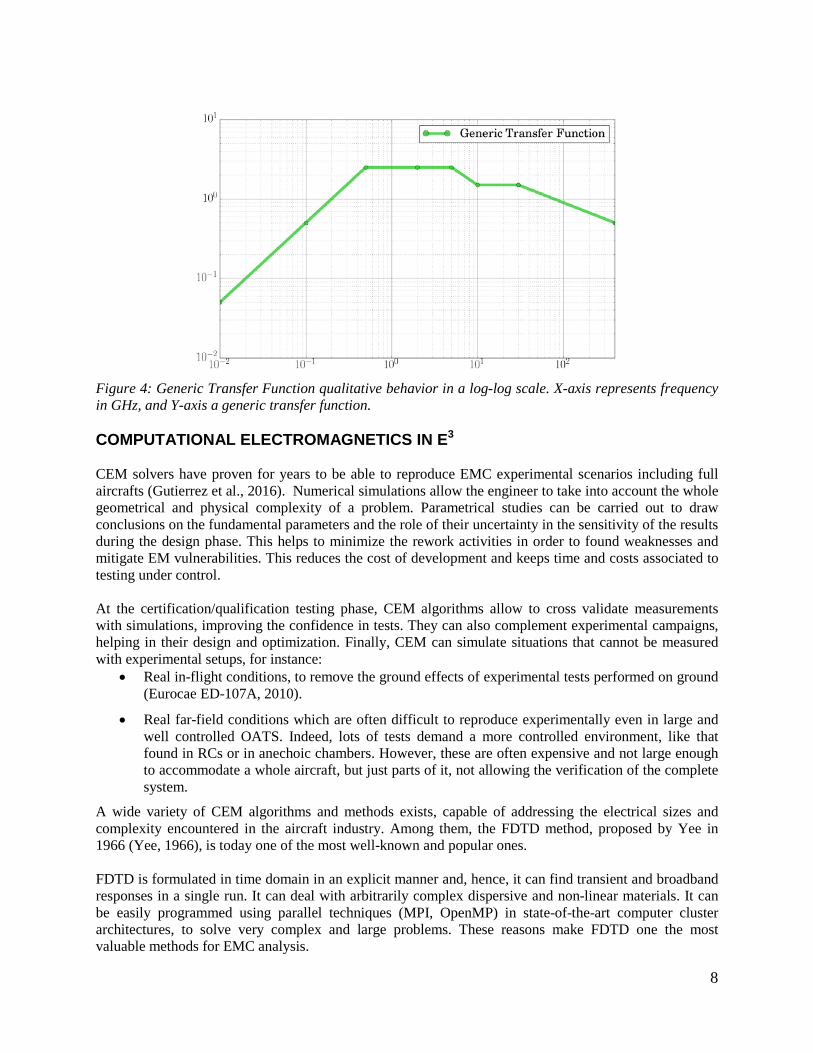
Transfer functions tend to have a common behavior, mainly depending on the aircraft size and well described in certification guides (Eurocae ED-107A, 2010) and (AC 20-158A, 2014). For instance, in DCI tests, the currents along cables inside a typical-size aircraft present the generic profile given in Figure 4 which has been obtained as the result of years of testing experience. We can distinguish three frequency bands which depend on the electric size of the aircraft and its apertures. EM fields in each band produce different electromagnetic coupling effects inside and on the fuselage (Rasek & Gabrisak, 2011; Schroder et al., 2014, Rasek et al., 2015; Parmantier et al., 2012):

• Low Frequency ( )10kHz,50MHz . In this range, the field penetration through the apertures is low and will mainly depend on the conductive properties of the fuselage. There are no resonances inside the aircraft, which behaves as a cavity under its cutoff frequency. The external EM fields induce strong surface currents flowing along its skin. These currents are inductively coupled to the internal cables which can be modeled by a simple LR series circuit in this range of frequencies. The characteristics of this circuit will depend on the geometry and position of the cables with respect to the apertures of the aircraft. When modeled in this way, the cutoff frequency of the transfer function is given by

cutoff 2 Rf

Lπ= (8)

where the resistance R depends on the conductivity and dimensions (length and section) of the cable and its loads, and the inductance is given by the cable dimensions (length and radius) and the distance of the cable to the current-return (e.g., the fuselage). Typically, the inductive part can be masked by low-resistive behavior due to low-loss cables, or cables being directly grounded to the fuselage.

• Medium Frequency ( )10MHz,100MHz . The apertures of the aircraft become more penetrable as frequency increases while the fuselage presents similar penetration characteristics to the low-frequency regime. The maximum coupling is reached at the firsts resonances of the aircraft structure or that of the wiring. This normally occurs when their size is a quarter or half the wavelength.

• High Frequency ( )100MHz,40GHz . In this band, the penetration through apertures of the EM energy into the fuselage is strong, dominating over the penetration trough the conductive skin. The surface current (jump between internal and external tangential magnetic field) on its skin diminishes. The field that penetrates into the fuselage may create destructive and constructive interferences, behaving as a reverberant cavity, which may even exceed the external field with very high peaks. This may suppose a major potential risk of this band, which affects the aircraft electronics devices directly.

8

Figure 4: Generic Transfer Function qualitative behavior in a log-log scale. X-axis represents frequency in GHz, and Y-axis a generic transfer function. COMPUTATIONAL ELECTROMAGNETICS IN E3 CEM solvers have proven for years to be able to reproduce EMC experimental scenarios including full aircrafts (Gutierrez et al., 2016). Numerical simulations allow the engineer to take into account the whole geometrical and physical complexity of a problem. Parametrical studies can be carried out to draw conclusions on the fundamental parameters and the role of their uncertainty in the sensitivity of the results during the design phase. This helps to minimize the rework activities in order to found weaknesses and mitigate EM vulnerabilities. This reduces the cost of development and keeps time and costs associated to testing under control. At the certification/qualification testing phase, CEM algorithms allow to cross validate measurements with simulations, improving the confidence in tests. They can also complement experimental campaigns, helping in their design and optimization. Finally, CEM can simulate situations that cannot be measured with experimental setups, for instance:

• Real in-flight conditions, to remove the ground effects of experimental tests performed on ground (Eurocae ED-107A, 2010).

• Real far-field conditions which are often difficult to reproduce experimentally even in large and well controlled OATS. Indeed, lots of tests demand a more controlled environment, like that found in RCs or in anechoic chambers. However, these are often expensive and not large enough to accommodate a whole aircraft, but just parts of it, not allowing the verification of the complete system.

A wide variety of CEM algorithms and methods exists, capable of addressing the electrical sizes and complexity encountered in the aircraft industry. Among them, the FDTD method, proposed by Yee in 1966 (Yee, 1966), is today one of the most well-known and popular ones. FDTD is formulated in time domain in an explicit manner and, hence, it can find transient and broadband responses in a single run. It can deal with arbitrarily complex dispersive and non-linear materials. It can be easily programmed using parallel techniques (MPI, OpenMP) in state-of-the-art computer cluster architectures, to solve very complex and large problems. These reasons make FDTD one the most valuable methods for EMC analysis.

9

FDTD FDTD and its main numerical features are well known in literature and they are part of most syllabuses in undergraduate studies. Some good references are the books (Taflove & Hagness, 2005; Yu, Mittra, Su, Liu & Yang, 2006; Sullivan, 2000; Kunz, Steich & Luebbers, 1993; Mittra, 2014). There is a vast literature exploring every single feature, formulating it to handle all kind of materials and boundary conditions, seeking for improved stability reformulations, searching for innovative meshing methodologies, etc. Particularly, hybridizations with other techniques allow the analysis of cable bundles and harnesses, an especially important topic in the context of EMC. Many of the published works are actually successful key advances in this matter. However, some of these methods are just not robust enough to be used beyond pure proofs of concept for academic examples and in no manner can be employed in problems of the complexity found in EMC in aeronautics. For this reason, just the basic fundamentals of FDTD are described, together with robust and accurate models to address EMC problems. Special attention is paid to our own ideas which allow handling aeronautic materials and cable bundles as they play an important role in the energy coupling inside an aircraft. FDTD fundamentals Maxwell’s curl equations in time domain can be written in a symmetric manner as

0

0

T

T

HE Mt

EH Jt

µ

ε

∂−∇× = +

∂∂

∇× = +∂

(9)

where 0 0,ε µ are the free-space permittivity and permeability, TJ

, TM

are the total electric and

magnetic current densities, E

and H

the electric and magnetic field vectors; all of them function of time and space ( ),r t . The total current densities include: the independent source current densities

source source,J M

, the polarization/magnetization current densities p p,J M

, in general dispersive and

anisotropic; and the ohmic conduction current density terms c c, MJ E M Hσ σ= =

source

source

T c p

T c p

M M M M

J J J J

= + +

= + +

(10)

These equations require, to be complete, the constitutive relationships relating the polarization and magnetization current densities with their causes. Typically, these are found in frequency domain as ) ) ( ) ,( ( ( () ) ( )p pJ j E M j Hω ωε ω ω ω ωµ ω ω= =

(11)

with ) ,( ( )ε ω µ ω being the constitutive parameters of the material. The frequency domain expressions (11) can be translated into time domain either if differential or convolutional form. A proper way of doing this is found in (Han, Dutton & Fan, 2006) where arbitrary dispersion is handled by expanding the constitutive parameters in arbitrary-order partial fraction pole/residue series found by vector fitting techniques (Gustavsen, 2006).

10

The classical FDTD method (Yee, 1966) employs centered operators to solve Maxwell’s equations (and the time-domain constitutive relationships) in Cartesian coordinates, by replacing the space and time derivatives by

( ) ( ) ( ),... ,... - / 2,...f f v v f v vv

νν

∂ + ∆ −∆≈

∂ ∆ (12)

This kind of discretization requires the space to be sampled in unit cells of sides ( , , )x y z∆ ∆ ∆ , in a not necessarily uniform grid, with the EM field-components placed in the well-known Yee’s cube staggered arrangement (Figure 5). The E and H-field components are also shifted in time by a Δ / 2t factor, yielding a final discrete explicit marching-on-in-time algorithm which finds the solution at a given time instant as a function of the solution at previous time steps.

Figure 5: Position of the EM fields in Yee’s cell (Reprinted from Cabello, (2017d)).

Just for illustration purposes, let us write the 1D FDTD equations for plain ohmic media

( )

( )

1 1/2 1/2, , 1/2 1/2

1/2 1/21/2 , 1/2 1/2 , 1/2 1

n n n ni a i i b i i i

n n n ni a i i b i i i

E C E C H H

H D H D E E

+ + +− +

+ −+ + + + +

= + −

= + − (13)

with

( )

( )

, ,

, 1/2 , 1/2, 1/2 , 1/2

, 1/2 1/2 1/2 , 1/2

2 Δ 2Δ, , /2 Δ Δ 2 Δ

2 Δ 2Δ, , /

2 Δ Δ 2 Δ

i ia i b i

i i i i

M i M ia i b i M M

M i i i M i

t tC Ct t

t tD D

t t

t t t ε σt ε t

t tt µ σ

t µ t+ +

+ ++ + + +

−= = =

+ +

−= = =

+ +

(14)

where Δi is the cell size at the space position i , and 1/2Δi+ is the cell-size of the dual mesh

defined by ( )1/2 1Δ Δ Δ / 2i i i+ += + . The subscript i denotes the space position ( Δx i= ), and the superscript n the time instant ( Δt n t= ). To find the constants in (14), a second-order5 centered average operator has also been employed to approximate the identity operator, so as to render a numerical scheme compatible with Yee’s space-time arrangement. In order to simulate open problems, proper reflectionless absorbing boundary conditions are required. A major breakthrough advance in FDTD was introduced in (Berenger, 1994) with the PML technique, capable of attaining reflections under 120 dB. PMLs have been extended to truncate almost any kind of material: dispersive, anisotropic, bianisotropic, metamaterials (Garcia et al., 1999, Taflove et al., 2013; 5 For a uniform discretization.

11

Hao et al., 2009). FDTD, endowed with PMLs, and dispersive material treatment, can handle almost any complex problem found in electrical engineering. A main restriction of the marching-on-in-time explicit algorithm (13) is that it requires the time step to be minored by the smallest space step of the spatial mesh to ensure its numerical stability. This is given by the well-known CFL or Von-Neumann criterion, which requires the so-called CFL Number to fulfil in 3D (Taflove & Hagness, 2005)

1

CFLN 11 1 1

i i i i

c t

Min x y z

−

∀

∆≡ ≤

+ + ∆ ∆ ∆

(15)

This reduces to CFLN 13

c t∆≡ ≤

∆ for a homogeneous isotropic mesh. The condition (15) relaxes in 1D

to

{ }

CFLN 1i

i

c tMin∀

∆≡ ≤

∆ (16)

Hence, a fine space discretization does not only imply an increase in computer memory, but also larger CPU simulation times6 due to the subsequent reduction in the time step. For homogeneous materials, typically a spatial resolution of 15-20 PPW at the maximum frequency provides enough accuracy7 (Taflove & Hagness, 2005)

max

Δ PPWc

f= (17)

However, when there are small geometrical features (edges, curvatures, slots, wires, thin panels…), all of them require being properly discretized-in-space, resulting into a global time step minored by the smallest space increment. This brute-force approach to deal with multiscale problems can imply huge-memory setups and long-lasting simulations, unaffordable even for modern computers. For this reason, sub-cell equivalent models are introduced. Some of them are:

• To handle curvature in a properly accurate manner without resorting to a dense mesh, conformal algorithms have proven to be useful. They are based on the use of the integral forms of Ampère and Faraday’s laws just locally in cells traversed by material interfaces. Refer to (Dey & Mittra 1997; Cabello et al., 2016) for more details. Other approaches include subgridding techniques combined with local time stepping schemes to mix meshes with different densities in the same simulation (Zivanovic et al., 1991).

• To deal with thin materials, like the CFC skin of an aircraft, NIBC can be used (Sarto, 1999). Another alternative referred to as SGBC, proposed by the authors in (Cabello et al., 2017a), is briefly described in the next sub-section.

6 We will not address here computer requirements issues, and the reader is referred to the cited literature. However, let us simply state that the current Xeon-Phi CPU MPI/OpenMP implementation of SEMBA-UGRFDTD scales at a speed of 2 Gcells/CPU. For instance, let us assume a 1 GCell problem (in the order of magnitude of those simulated in this chapter), meshed with space steps of 1 mm to reach 18 GHz. Using a typical CFLN=0.8, a physical time of

610 s− requires roughly 3 hours of CPU in 32 nodes of a modern supercomputer cluster (like the Marconi KNL one that we currently employ). 7 Note that the condition (15) implies that good space resolutions automatically yield good resolutions in time.

12

• To handle cable bundles, once again brute-force meshing is not the solution. In the last sub-section of this section, the authors present a hybrid MTLN based in (Berenger, 2000) hybrid method, that can also be extended to cables not aligned with the Cartesian grid (Guiffaut et al., 2010).

Though further details will not be provided here, there are many other situations also requiring sub-cell treatment in FDTD: thin slots, junctions, gaskets, etc. All of them are important in EMC, as they are responsible of coupling EM energy inside the aircraft. Subcell models of lossy thin panels Conductive thin panels (metallic, CFC, etc.) are part of the skin of an aircraft. These can be very complex, usually multilayered, anisotropic and frequency dispersive. Typically they are much thinner than usual mesh sizes, and hence they cannot be resolved by the usual FDTD scheme as this would imply using unaffordable large meshes. In this section, the authors briefly describe the SGBC technique proposed in (Cabello et al., 2017a, Cabello et al., 2017b), which hybridizes a 1D Crank-Nicolson FDTD scheme to deal with the field propagation inside the thin-panel, with the usual 3D Yee- FDTD scheme for the rest of the problem. SGBC has been used in all the simulations presented in the last part of this chapter to model the composite parts of the aircrafts. SGBC starts from the same assumption made by NIBC (Sarto, 1999). It postulates that plane waves impinging on a conductive planar thin-panel with oblique incidence, refract at a close-to-normal angle regardless of the actual angle of incidence, as far as the refractive index is much higher inside the thin-panel than outside. It can be easily proven that for grazing incidence / 2iθ π→ (the worst-case), the

wave refracts at an angle 2| | 10tθ−< with the normal if

[GHz] 1.8 [kS/m]f σ< (18) This means that for the typical conductivities ( 410 S/mσ > ) of the panels found in automotive or aeronautics, the model holds up to 18 GHz regardless of the panel thickness. Let us briefly describe the SGBC method for a simple isotropic planar ohmic thin panel, of thickness th , aligned with a Cartesian plane8, having a constant conductivity, embedded in free space. First, the thin-panel is sub-gridded into N 1D FDTD-cells of size fineΔ , according to the setup of Figure 6. The outer 3D FDTD cell size is coarse fineΔ Δ> . Next, the tangential E-fields on each side of the thin-panel 1 2,S SE E are duplicated at the usual 3D Yee position, to account for each face value, which are employed accordingly to update the magnetic field component at each side 1 2,S SH H by using the integral form of Ampère’s law. The SGBC algorithm continues as follows:

1. The fields inside the panel domain denoted by ,nL iE , , 1/2

nL iH + are updated by a Crank-Nicolson

1D scheme (CNTD) (Yang et al., 2006), which is just an unconditionally stable variation of the Yee FDTD scheme, maintaining is the usual space staggering, but co-locating the E and H-fields in time by means of an average operator

8It can easily be formulated also in a conformal manner to handle curved materials.

13

1 1, , 1 , , 11

, 1/2 , 1/2 , 1/2 , 1/2

1 1, 1/2 , 1/2 , 1/2 , 1/21

, , , ,

2

2

n n n nL i L i L i L in n

L i a i L i b i

n n n nL i L i L i L in n

L i a i L i b i

E E E EH D H D

H H H HE C E C

+ ++ ++

+ + + +

+ +− + − ++

− −= +

− −= +

+

+ (19)

Unlike for 1D Yee-FDTD, the resulting marching-on-in-time scheme (19) is now implicit, but it can be easily transformed to yield a simple tridiagonal system of equations in E, and an explicit equation for H. Refer to (Cabello et al., 2017a) for details.

2. E-fields and H-fields outside the thin-panel are advanced in the usual 3D Yee-FDTD manner.

3. The connection between the coarse and fine mesh is made through a hybrid implicit-explicit (HIE) method described in detail in (Cabello et al., 2017a).

Figure 6: Cross section of a FDTD cell with a SGBC boundary and details of the thin-panel subgridding (Reprinted from (Cabello et al., 2017b) ©2017 IEEE, with permission from IEEE).

SGBC has been introduced as a robustly stable replacement of NIBC which was often reported to exhibit late-time instabilities (Kobidze, 2010; Nayyeri et al., 2013). Some of its characteristics are:

• SGBC has exhibited a strong late-time stability for all the cases that we have simulated, whereas NIBC has often run into late-time instabilities, sometimes requiring heuristic time-step reductions of up to 1% that of the analytical limit (15).

• The unconditional stability of CNTD allows us to choose the time step just constrained by the exterior coarse discretization (15).

• The computational overburden of solving the 1D tridiagonal system of equations does not compromise the computational efficiency of the full problem.

• The extension of this method to anisotropic materials would no longer be affordable by 2D CNTD. Proper variations of it, like a 2D Alternating Direction Implicit FDTD (Garcia et al., 20007), also unconditionally stable, can be an alternative.

• Instead of a 1D CNTD method, a pure 1D Yee-FDTD method could also have been used inside the slab by employing an ETD method like that described in (Cabello et al., 2017c ), not requiring dramatic reductions in the times step (50% that of Eq. (15) for moderately conductive media).

14

Hence, a 2D Yee-FDTD method could also be an affordable alternative to 2D CNTD to address anisotropic lossy panels.

• Often the internal nature of the multilayered lossy thin panel is not known, but just the S-parameters, either found from measurements, or from microscopic assumptions. In this case, SGBC could still be used by retrieving effective macroscopic constitutive parameters following the roadmap described in (Cabello et al., 2017b).

Subcell models of cables Cables are the main characters responsible for coupling EMI inside the equipment that they interconnect. Their accurate simulation is a must, and again meshing them by brute in FDTD, is not computationally viable. The MTLN equations are the appropriate alternative to deal with cable-bundle waveguiding analysis. When they are coupled to Maxwell’s space-time curl equations, they provide a way to analyze the cable-bundle behavior inside a complex inhomogeneous 3D EM environment. A typical implementation of a coupled FDTD-MTLN method is based on (Berenger, 2000), which extends the thin-wire approach of (Holland, 1981), to many-wire bundles, by taking into account the cross-talk between the individual wires. It can also be generalized using the ideas of (Guiffaut, 2012; Ledfelt, 2001; Edelvik, 2002) to permit the treatment of wires not aligned with the Cartesian FDTD grid. Just as a reminder, let us recall the coupled FDTD-MTLN Holland equations for a single wire with a p.u.l. resistance R running along the x-direction in free space

0

0x t

x t x

y z z y t x

I C VV L I R I E

H H Eε

∂ + ∂ =

∂ + ∂ + =

⇑⇓∂ −∂ = ∂

(20)

where the p.u.l. inductance L, and the capacitance C, fulfill the usual 2LC c−= relationship. In Eq. (20) the inductance L is found with respect to an infinite coaxial current return, which, in FDTD, leads to an expression depending on the space step and the wire radius. The maximum time-step for stability of the coupled scheme is proven to depend on L (Schmidt & Lazzi, 2004) and to be minored by the wire radius, which cannot be larger than half the space step. For wire bundles, this upper limit translates, roughly speaking, into that of a circumference enclosing the whole bundle. Hence, in practice the FDTD-MTLN Holland-Berenger method is often applied at cable-overbraid level, to find the currents flowing along the outermost sheath. Next, these currents are used to find the currents inside the bundle by using the transfer impedance (Feliziani & Maradei, 2002), found by using measurements, or analytical formulas (Vance, 1974; Yatsenko et al., 2000). The limitation on the stability constraints imposed by the fully coupled MTLN-FDTD method also can be removed by using a pure field to transmission line (field-to-TL) model (Agrawal, et al., 1980). This may seem a simplification of the fully coupled technique in the sense that it just takes into account the coupling of the external field found by FDTD to the cables, without coupling back the currents flowing along the bundle wires to the FDTD domain (just the up-to-down coupling is kept in Eq. (20). However, field-to-TL is in no manner an approximation and becomes an exact application of Huygens’s equivalence principle, when only TL modes are assumed to be present (Rachidi, 2012). However, concerns are raised when the current return is not perfect (for instance due to interruptions of the overbraid), and the structure (e.g. the fuselage in case of an aircraft) provides the current return instead. For these cases, the FDTD-MTLN Holland-Berenger formulation would provide a more convenient approach.

15

Modeling of reverberation chambers

RCs are highly-resonant overmoded metallic cavities which are large enough to accumulate enough statistically independent modes at low frequencies (Besnier & Demoulin, 2011). They typically have a mechanical stirrer that rotates to change the modal distribution inside the cavity for obtaining an average uniform field throughout on the volume occupied by the device under test. The international standards recommend at least 60 transmission modes for considering a reverberation environment (IEC 61000-4-21 Ed2, 2011 and IEEE 299.1, 2013). In the case of a cubic reverberation chamber, the number of modes can be written as function of frequency (Hill D.A., 2009):

( ) ( )3

3

8 13 2S

f fN f abc a b cv v

π= − + + + (21)

where a,b,d are rectangular chamber dimensions, ν is the speed of light, and f is the chamber source frequency. The numerical simulation of several stirrer positions inside an electrically large cavity is unaffordable for a time-domain solver. However, an equivalent model can be used by employing a superposition set of plane waves with a random uniform statistical distribution on their polarization, delays and direction of incidence (Hill D.A., 1998; Moglie & Pastore, 2006). Instead of a PEC cavity, the computational space can then be truncated by usual PML as absorbing boundary conditions and affordable simulations can be done. Each plane wave is inserted in FDTD by using the total field/scattered field formulation of (Taflove & Hagness, 2005) based in Huygens’ equivalence principle. CAD CLEANING, SIMPLIFICATION AND MESHING

In the previous section, we have described some of the basic desirable features that a numerical FDTD solver must include to be able to carry out EMC analysis of full aircrafts in a computationally affordable manner. To this end, some preliminary simplifications of the aircraft model need to be done to get the final numerical input for the solver. The starting digital mock-up provided by a CAD tool (Figure 2) is often too complex to be meshed and be directly used in the simulation. This is a crucial stage, since simulation results, and CPU times strongly rely on the quality of the numerical model fed to the solver: mesh, cables, sub-cell details, etc. In this section, we briefly discuss this process.

Figure 7: a) Isometric view of the digital mock-up of an AIRBUS C-295 aircraft, with a detailed view of the cockpit. b) Simplified geometry with a detailed view of the cockpit (aerodynamic surfaces are depicted

16

with a degree of transparency to allow the observation of the internal surfaces). (Reprinted from (Gutierrez et al., 2014) ©2014 IEEE, with permission from IEEE). Typical CAD models include an unnecessary level of geometrical details from the EM point of view when they are provided by the mechanical engineering departments. Therefore, the simplification, cleaning, and meshing of complex CAD models is a very important part of the EMC simulation process in order to provide a mesh that can be fed to the EM solver. The main tasks of cleaning, simplification and defeaturing can be summarized as follows:

1. Solve typical problems in CAD models as lack of connectivity, bad or non-existing topology, bad

definition of parametrical surfaces, residual curves from intersections...

2. Remove those pieces or details that are not involved in the simulation, either according to their electrical size (screws, rivets …) or to their composition, for instance, often lossless materials can be discarded.

3. Replace the complex parts with simpler ones able to represent with enough accuracy the reality from the point of view of the EM interactions.

4. Maintain the ohmic connections/disconnections: Sometimes the separation between objects must be increased to the cell size to avoid a false electrical connection in the mesh, some other times physically connected parts appear unconnected in the CAD file and must be fixed.

5. Dimension degeneration. One side of a 3D object can be reduced to a point when it is smaller than one cell size, implying a reduction on its dimensionality. For instance, a 3D panel thinner than the mesh size would be replaced by a 2D surface; in the same way cables and pipes which their section smaller than the cell size can be replaced by lines. This fact must be taken into account when the CAD model is treated because the dimensionality of an object restricts the models that can be used with it.

Obtaining a new geometry which is simpler than the original one but still able to capture the EM reality is a very time-consuming task. This phase requires experienced engineers with a good knowledge of the involved physics and with a deep understanding of the mesher and solver capabilities (Gil & Gutierrez, 2011, Gutierrez et al., 2014). We can see in Figure 7(b) the result of this process for the C-295 aircraft, which has led a reduction by a factor 500 in the size of the final CAD file, making it possible to be meshed and simulated. For FDTD, the simulation mesh is typically obtained by a Cartesian mesher which converts a mesh of triangles/tetrahedrons into the voxels, surfels and linels which are handled by the FDTD method. This procedure automatically filters out sub-cell details, including those may be relevant from the EM point of view (thin panels, wires, slots, etc.). Special care must be taken to prevent this situation, and to assign explicitly appropriate material properties to model these details appropriately. Numerical models: materials Materials with low conductivities can be assumed to be equivalent to free space and removed from the model, e.g., lossless air-like dielectrics, like plain fiberglass parts. On the other hand, materials with high conductivities, that when shaped as panels provide a SE over than 100 dB can be directly modeled as PEC surfaces, this includes most metals or composites which are reinforced with aluminum foils. CFC panels are typically formed by multilayered plies of carbon fibers immersed in a matrix medium. They require a careful analysis to incorporate proper equivalent models of their macroscopic behavior.

17

These models typically have a SE with a constant low-frequency profile which then increases with frequency due to skin-depth effects up to a certain maximum. After this maximum is reached, the SE may decay asymptotically due to the presence of inductive effects in the conductive fiber. Depending on the position of that maximum, either a plain homogeneous ohmic model, or a more complex dispersive one, must be employed. This analysis can typically be performed by looking at the microscopic geometrical properties of the panel: random, woven, non-woven, periodicity, number of layers, fiber density and orientation, conductivity of fibers, reinforcing meshes, etc. Several models are available to predict its shielding capabilities, or by measuring it with proper fixtures (Sarto et al., 2014). Regarding apertures, they must be carefully handled, since they represent entry points of EM energy. Holes, gaps between different panels, thin slots, etc., can be treated as free space if their dimension is larger or comparable to the cell size. Otherwise, these must be managed by appropriate sub-cell models (Gkatzianas & Tsiboukis, 2003). Finally, an important aspect in any numerical model is the effect of small variations or uncertainties in the different physical parameters, e.g., position of cables, material properties, etc. This becomes apparent even at experimental level when data from different specimens of the same AV or from different test campaigns are compared and a disagreement is found for quantities that otherwise should coincide. A way to assess these uncertainties is to apply a statistical analysis by taking into account the variability of all the AV parameters. For instance, heuristic approaches based on an affordable set of simulations chosen as representative according to the engineer experience, can be used to analyze the impact of the inclusion of installations, the maintenance of electrical contacts, the assignation of materials, the selection of appropriate cables with their significant properties, etc. From the different simulations, the sensitivity of the simulation results to variations in the EM model can be derived. Next, theoretical guidelines can be drafted with quantitative notions of the error magnitudes introduced with these approximations. As a result, an increase in the reliability of the simulation results can be achieved in order to use them in a certification process. VALIDATIONS METHODS The workflow in Figure 2 ends with the validation of the numerical results against experimental data. Validation methods are necessary to objectively evaluate the similarity between different datasets. Although in many fields of research, a simple visual inspection is used as the validation method, numerous studies show that a direct comparison point-by-point is not feasible when large amounts of data are compared. Therefore, this method is not recommended to validate the results and much less to assign an absolute value of accuracy. This approach makes sense only for simple models, but in EMC simulations, the results are often very complex. Feature selective validation In the last years, several validation methods evaluating the similarity between measures, imitating the opinion of EMC experts have been developed: correlation, reliability factor, integrated error log frequency, etc. One of the most widely used, for its versatility and simplicity, is the FSV method based in IEEE 1597.1/2 standard (IEEE Std 1597.1, 2008; IEEE Std 1597.2, 2010). This method allows us the comparison to be quantified objectively, removing the element of subjectivity from the decision making process.

18

FSV has the advantage of analyzing the two major aspects that are widely considered paramount in any validation: the magnitude levels and the shape of the dataset graphs. It is based on the decomposition of the results into two groups; the first one discusses the difference in amplitude (ADM) and the second one the difference between the characteristic of the signals (FDM). The combination of these two indicators is a new indicator named GDM that measures the overall difference between both datasets (Duffy et al., 2006; Orlandi et al., 2006). All these indicators (ADM, FDM and GDM) have the ability to be configured to perform a point-to-point analysis. The advantage of relying on a point-to-point data is to know which areas of the data sets have the major differences. Another way to qualitatively analyze the FSV indicators is represented by a probability density function which is useful for a rapid and comprehensive analysis of the results. This indicator uses a histogram that can be divided into six categories: excellent, very good, good, fair, poor, and very poor, according to the IEEE standard (IEEE Std 1597.1, 2008) (Figure 8). In the simulations described in the last part of this chapter, the FSV tool proposed in (Jauregui et al., 2010; Jauregui et al., 2013; Jauregui et al., 2014a) has been employed for validation9. With the aim of considering the most relevant data of the measurements and the simulations, several enhanced techniques can be used. The first one is a technique to provide equivalent uncertainty estimation in the FSV validation method (Jauregui et al., 2013). This technique uses the level of uncertainty of one of the datasets, typically the measurements, to find an equivalent tolerance for the validation method. Another technique is to take into account a relative level in the comparison process. Because in many EMC cases the comparison analysis is focused on a certain level and ignores much of the data, this technique relies in the idea of weighting the different indicators of the traditional FSV method (Jauregui et al., 2014b). The weighting function may be changed to accomplish the application-specific needs of the case which is being validated, avoiding erroneous decisions on the final results.

9 The GVT FSV tool of the UPC can be freely downloaded from http://www.upc.edu/web/gcem/.

19

Are there about thesame number of similarities

and differences?

Are there more differencesthan similarities?

No

Yes

Yes

Manydissimilarities

Some similarities

Many similaritiesMore similarities

No

Very poorVirtually nodiscernable agreement 6

Minor agreement

Reasonableagreement over many

portions of the dataGenerally good

agreement across thedata

Minor variationsallowable

Perfect or almostperfect match

Poor

Fair

Good

Very good

Excellent

5

4

3

2

1

Start

Figure 8: Confidence histogram rules [IEE-5971] APPLICATION CASE 1: C-295, NUMERICAL ASSESSMENT OF HIRF EFFECTS In the remainder of this chapter the authors will describe the process carried out for the virtual testing of a series of complex AV EMC scenarios. The first of this series consists of a C-295 aircraft from AIRBUS under HIRF conditions, presented in (Gutierrez et al., 2014) by some of the authors of this chapter. The C-295 is a medium-weight transport aircraft. It employs standard aeronautic materials. The most relevant conductive ones, compliant with MIL-HDBK-5H (1998), are: aluminum alloys (2024, 6061, 7075, 7050), ferrous alloys (DAISI 4340, AISI 321, PH 13-8Mo.), and titanium alloys (Ti6Al4V). Its fuselage is mostly metallic, which makes it robust against external electromagnetic threats. The engine nacelles, some parts of the central wing, the landing gear sponsons, small pieces in the stabilizers and wings, are all taken as PEC. Composite materials are also employed, mainly carbon fiber and fiberglass e.g. the radome is a sandwich-type structure with outer fiberglass laminates. Around 20% of the C-295 composition is based in CFCs. Leaks from EM fields and currents are mainly due to apertures around hatches, joints, hinges and the use of non-conductive materials in radomes, fairings, windows, etc. The experimental setup consisted of a radiated LLSF test, carried out in the Airbus OATS in Getafe (Spain), consisting of a circular platform 90 m in diameter, made of concrete reinforced with an embedded metallic grid. The aircraft is radiated (far-field regime) with proper antennas between 100 MHz and 18 GHz. Care is taken to let at least 50 meters between the aircraft and any other source of EM noise, including any object able to create undesired reflections (see Figure 9). The tests were carried out according to (Eurocae ED-107A, 2010).

20

Figure 9: LLSF Tests at Airbus Military OATS Facility (left). Electric Field measurements during LLSF Tests. (right). (Reprinted from (Gutierrez et al., 2014) ©2014 IEEE, with permission from IEEE). First of all, the calibration field is measured in free-space with the probes located at the six points that they will occupy in the LLSF test of the aircraft. Next, the same data is recorded at the same points within the aircraft, and normalized to the calibration levels. Two of these test-points are inside the cockpit, three in cargo bay, and one in the engine. In order to get the worst case for the coupling through the aircraft slots and apertures, several angles and polarizations are employed to radiate each zone. For this, the maximum field level is found at each frequency and the envelope of all of them is found along the frequency band.

Modeling and simulation approaches

The FDTD-MTLN Holland-Berenger model of SEMBA-UGRFDTD is used to deal with cable bundles and/or cable overbraids, and the SGBC method to handle electrically thin composites. The mesh employs a uniform cell size of 20 mm which yields a problem with 734 Mcells (1228 x 1307 x 459). A time step 80% that of the CFL limit has been taken ( 1230 10−⋅ s) to comply with cable-bundle stabilities mentioned earlier in this chapter. This discretization allows us to achieve a maximum of frequency of 10 GHz (instead of the 18 GHz achieved with measurements), since the resolution reaches the limit of PPW=15 cells/wavelength (in free space), to consider results accurate. Hence, a Gaussian modulated plane-wave, with a frequency range between 100 MHz and 10 GHz, is used to illuminate the aircraft, mimicking the antenna radiation. This will also have impact in the results, as will be seen later, in some mismatches between 100 and 200 MHz, where the far-field assumption for the antennas is in its validity limit. Finally, the model is truncated by means of PML boundary conditions. For validation the FSV methodology has been employed. Additionally, results with a PFC used for validation under the HIRF-SE project will also be shown. The procedure to get the PFC results is summarized as follows.

1. A set of seven observation points occupying the volume of the receiving antenna is used to probe the EM field through an average operation. This process obtains a better representation of the receiving antenna used during the tests.

21

2. A minimum of 100 frequencies per decade above 100 kHz equally spaced on a log scale is measured.

3. The raw data is filtered by using an averaging bandwidth of 5% of the frequency of interest, as recommended in (Eurocae ED-107A, 2010, section 6.4.5).

4. The maximum value frequency-by-frequency considering all illumination angles and both polarizations, for each point, is calculated, and taken as the WC results.

5. The maximum values of the WC, within a sliding frequency window of 10% of the central frequency, are used to find the data envelopes. This permits to account for any shift in resonances between the aircraft installation and the modeled test setup.

6. Finally, the value of the difference between simulation and measurement in dB is calculated.

7. The data are assumed to pass the criterion if this difference falls below 6 dB.

Figure 10: C-295 cockpit unstructured mesh (left). Cartesian mesh of the engine (right). (Reprinted from (Gutierrez et al., 2014) ©2014 IEEE, with permission from IEEE). Results

The transfer function for the electric field at 3 test points is shown in Figure 11, Figure 12, and Figure 13, comparing the worst-case numerical/experimental transfer function, as well as the envelopes resulting from the application of a sliding frequency window. It bears noticing that numerical and experimental envelopes are within a 6± dB range for most of the frequencies. Table 1 shows the PFC results for all the six points. The FSV methodology has also been applied to the worst-case curves for comparison, finding fair agreements, in general (Table 2). To become aware of the quality of experimental/numerical results matching in ±6 dB range, we have conducted another comparison with data found in two different test campaigns, with two different C-295 aircrafts, and different antennas and equipment. A point in the cockpit has just been taken and results are plot in Figure 14. It bears noticing that a similar ±6 dB matching pencil is also found in measurement/measurement comparisons. Fair agreement is also found by FSV, though not shown here, between experimental/experimental data. This provides a good idea of the real uncertainty of this kind of EMC problems, and points out the way for revisiting the FSV standard (IEEE Std 1597.2, 2010; Jauregui et al., 2014) to yield rates adapted for this specific topic.

22

Figure 11: a) Comparison between measurements and simulations for the test point 1 located in the cockpit. b) Difference between simulation and measurement and 6 dB limit. (Reprinted from (Gutierrez et al., 2014) ©2014 IEEE, with permission from IEEE).

23

Figure 12: a) Comparison between measurements and simulations for the test point 3 located in the cargo bay. b) Difference between simulation and measurement and 6 dB limit. (Reprinted from (Gutierrez et al., 2014) ©2014 IEEE, with permission from IEEE).

Figure 13: a) Comparison between measurements and simulations for the test point 6 located in the engine. b) Difference between simulation and measurement and 6 dB limit. (Reprinted from (Gutierrez et al., 2014) ©2014 IEEE, with permission from IEEE).

Table 1. PFC results for the UGRFDTD code. Percentage of points inside the limit, greatest difference

between envelopes and mean difference between envelopes. (Reprinted from (Gutierrez et al., 2014) ©2014 IEEE, with permission from IEEE).

Pass/Fail Criterion Points inside Limit Greatest Difference Mean Difference

Test Point 1 88% -7.65 0.51 Test Point 2 89% 16.29 1.03 Test Point 3 94% -10.44 -1.34 Test Point 4 81% -14.41 -2.52 Test Point 5 76% -12.20 -1.55 Test Point 6 100% -5.95 -1.41

Table 2. FSV results for the C-295 test-case. (Reprinted from (Gutierrez et al., 2014) ©2014 IEEE, with

permission from IEEE).

FSV GDM ADM FDM Test Point 1 0.9936 0.6123 0.6880 Test Point 2 0.7764 0.4588 0.5896 Test Point 3 0.7689 0.4640 0.5572 Test Point 4 0.7943 0.5702 0.5042 Test Point 5 0.8357 0.4876 0.5682 Test Point 6 0.6295 0.3418 0.4934

24

Figure 14: a) Comparison between two measurements on a point in the C-295 cockpit from different test campaigns. b) Difference between the two measurements and 6 dB limit. (Reprinted from (Gutierrez et al., 2014) ©2014 IEEE, with permission from IEEE).

APPLICATION CASE 2: MILANO CENTRAL FUSELAGE IN A REVERBERATION CHAMBER, A TEST-SETUP TO ASSESS HIRF EFFECTS

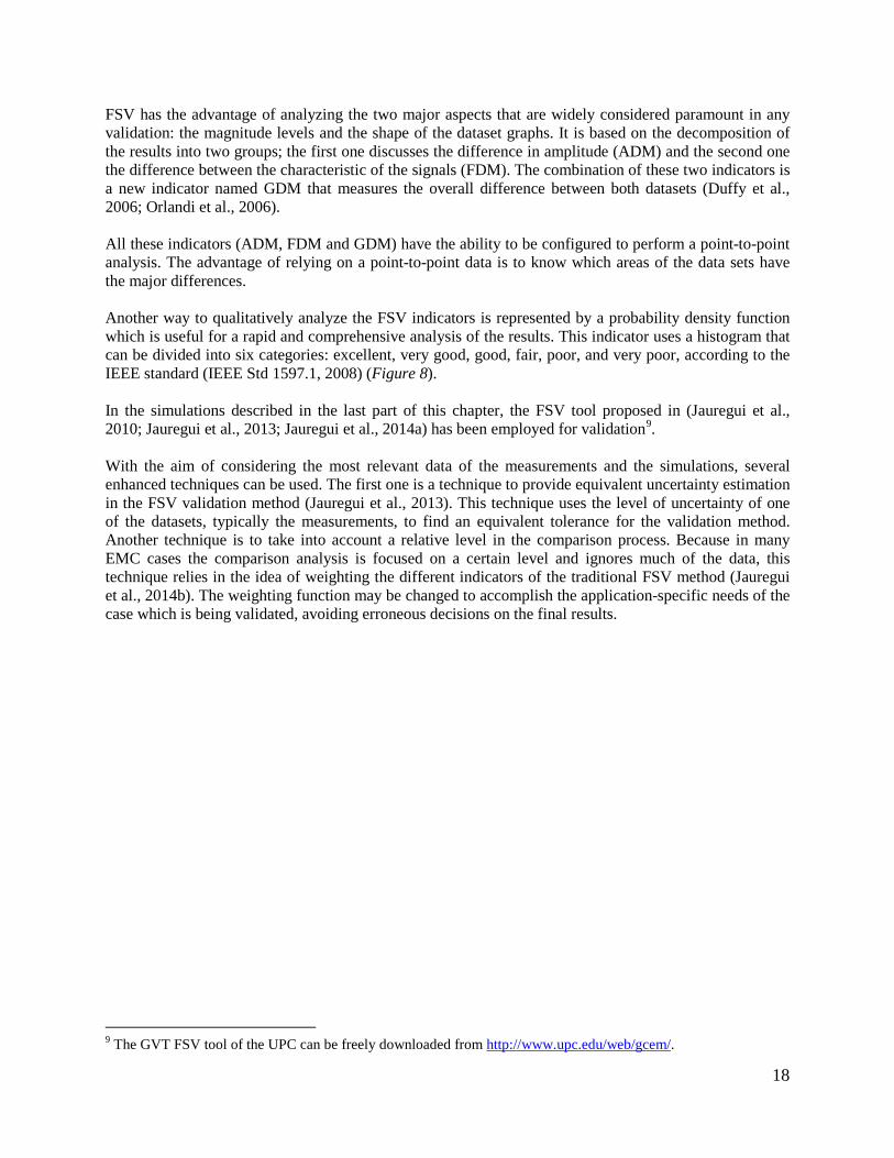
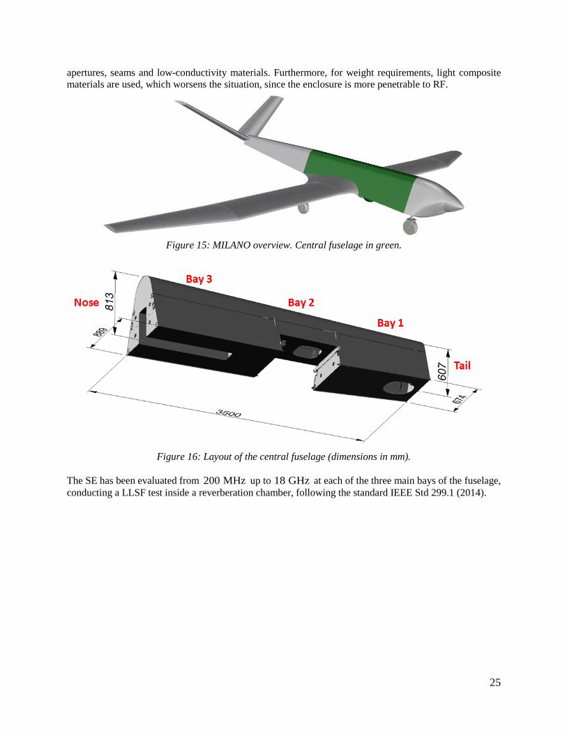
The next test-case consists of the central fuselage of the MILANO UAV. This platform is a medium altitude long endurance remote piloted aircraft system developed by INTA. The MILANO UAV, made mostly in carbon-fiber composite, has a wingspan of 12.5 m, a length of 8.52 m and a height of 1.43 m. The UAV structure consists of independent composite modules with metallic fittings in order to assemble and disassemble the aircraft for transport. Only the central fuselage was used for the work described in this section, in green in Figure 15. Its top fairing that can be removed, exposing then three different bays or compartments. The big apertures of the central fuselage located at the bottom, left hand side and right hand side (see Figure 16) are covered with metallic plates. The MILANO UAV is suited to hold equipment usually classified as Design Assurance Level A10. Hence, this equipment requires very high level of protection. The best solution is to home it within highly shielded enclosures. However, in practice, there is also a degradation of the shielding mainly due to

10 DAL-A, Catastrophic: The failure of systems in that level would prevent the safe operation of the aircraft.

25

apertures, seams and low-conductivity materials. Furthermore, for weight requirements, light composite materials are used, which worsens the situation, since the enclosure is more penetrable to RF.

Figure 15: MILANO overview. Central fuselage in green.

Figure 16: Layout of the central fuselage (dimensions in mm).

The SE has been evaluated from 200 MHz up to 18 GHz at each of the three main bays of the fuselage, conducting a LLSF test inside a reverberation chamber, following the standard IEEE Std 299.1 (2014).

26

Figure 17: Overview of front part inside the RC

Figure 18: Example of a probe (at P2)

Modeling and simulation approaches The CAD data was prepared, simplified and meshed by using the methodology described earlier in this chapter. The cubic-cell mesh has a constant space-step of 1 mm, which allows us to have PPW=17 cells/wavelength in free space at the upper frequency limit of 18 GHz. A problem with 5.2 GCells is yielded (3822 x 1205 x 1135). In our case, the fuselage incorporates just two kinds of materials: PEC and CFC. The CFC material has been taken as a homogeneous conductive thin-panel, 2.5 mm thick, and a conductivity of 10 kS / m . The Shielding effectiveness of a planar slab made on this CFC is illustrated in Figure 19. We have employed the SGBC method to simulate it with SEMBA-UGRFDTD. PML boundary conditions are used to truncate the model.

27

Figure 19: Shielding effectiveness of a planar slab of the Milano CFC. For the source, the RC model describer earlier in this chapter has been used. A Gaussian-modulated time-profile covering the frequency range has been taken. Results The SE was evaluated at three observation positions, one at the center of each bay. Results with SEMBA-UGRFDTD solver and experimental data are shown in Figure 20, Figure 21 and Figure 22. The results show a reasonable agreement at each probe position.

Figure 20: Shielding effectiveness at P1

28

Figure 21: Shielding effectiveness at P2.

Figure 22: Shielding effectiveness at P3 APPLICATION CASE 3: SIVA, A DCI TEST-CASE TO ASSESS LIE EFFECTS

The last case presents the experimental arrangement for the SIVA UAV, published in (Cabello et al., 2017c) by most of the authors of this chapter. This set-up has been tested with the DCI procedure in a LLDD setup (Figure 23). Results are shown mainly for the LIE frequency band and compared to experimental data conducted by INTA. The SIVA system consists of a ground-control station plus an UAV mostly made in CFC and fiberglass. It has a wingspan of 5.81 m, a length of 4.025 m, and a height of 1.63 m. For this UAV, in the absence of large apertures, otherwise usual in typical aircrafts, the main mechanisms of EM energy entrance are due to apertures covered by fiberglass (radomes, fairings), hatches, joints, and hinges, and through the CFC materials themselves.

29

Figure 23: DCI test setup using coaxial return of SIVA-UAV in INTA’s OATS. (Reprinted from (Cabello et al., 2017c) ©2017 IEEE, with permission from IEEE). Experimental data for the DCI test setup of Figure 23 measured in INTA’s OATS have been used for validation. The spacing between the metallic wires of the cage return network is 30 cm. They are separated 63 cm from the UAV upper surface, and 37 cm for the lower surface. The RF power was injected through 2 wires connected to the propeller screws. The injected current was measured and recorded for normalization of the current induced on different cables installed inside the UAV, located in four positions (Figure 24). Most SIVA equipment was removed, keeping just four representative ones for our validation purposes: the FTCU, the PCU, the Airbag Bottle and the wings lights, together with the three cable bundles routed among them.

Figure 24: DCI probes: CP1, CP3, CP5, and CP7. (Reprinted from (Cabello et al., 2017c) ©2017 IEEE, with permission from IEEE).

30

Modeling and simulation approaches The original CAD model Figure 25 has been cleaned up and defeatured, according to guidelines given earlier in this chapter, to yield the simplified model of Figure 26 . It has been meshed with a uniform isotropic grid of 6 mm space-step for the UAV region, combined with a non-uniform one ending into a 20 mm space step at the PML boundaries (Figure 27), resulting into a very well resolved problem at the upper 200 MHz frequency: 75 cells/wavelength in free-space. A 160 Mcells (1168 x 498 x 277) model is finally yielded. The time step corresponds to a CFLN=0.75, imposed by the thin-wire hybrid FDTD solver stability condition.

Figure 25: Original CAD model including all geometrical details (Reprinted from (Cabello et al., 2017c) ©2017 IEEE, with permission from IEEE).

Figure 26: CAD model simplified after cleaning and including equipment and current probe locations. (Reprinted from (Cabello et al., 2017c) ©2017 IEEE, with permission from IEEE).

31

Figure 27: General and zoom views of final FDTD mesh. The upper right inset shows the DCI injection wires attached to the nose and tail of the UAV. In red the internal wire bundles. (Reprinted from (Cabello et al., 2017c) ©2017 IEEE, with permission from IEEE).

Regarding the materials, just CFC ones were maintained, while fiberglass ones were removed. The equipment PCU, FTCU, airbag bottle (Figure 25) have been modeled as PEC. The UAV skin is a CFC, assumed to have a constant conductivity of 10 kS/m and an average thickness of 0.92 mm, treated by the SGBC method in SEMBA-UGRFDTD. Cables and bundles inside the UAV employ the FDTD-MTLM Holland-Berenger method. Only representative cables have been kept: the one from the FTCU to igniter harness, and the one from the wing light to the PCU, including their resistive ending connectors. For the numerical simulations of the DCI test, the current is directly injected through the cable at the attachment point Figure 23 . The cable at the exit point has a lumped resistance of50 Ω . A Gaussian signal with -3 dB decay at 400 MHz is fed as a voltage source in a thin wire located at the beginning of the coaxial return. The surfaces and lines of the coaxial return array have been modeled as PEC lines. The OATS concrete ground is also included in the numerical model, though the results in this frequency range are insensitive to this, for being a DCI test-setup and field is assumed to be confined into the system formed by the fuselage and the coaxial return. For validation the FSV methodology has been employed.

Results The induced current at different probes (CP1, CP3, CP5, CP7 (See Figure 24, Figure 26)) are evaluated (Figure 28, Figure 29, Figure 30, Figure 31) and their values normalized in the frequency domain with

respect to the injected current to find the transfer function as 1020 log cabledB

injected

IT

I= .

We can appreciate a low-frequency inductive trend at the points CP1, CP3, CP7, since these cables are being grounded through a resistive connector to the fuselage. However CP5 was directly grounded in the

32

experimental setup, but the numerical model made use mistakenly of a grounding resistance. This explains the constant trend in the experimental transfer function at low frequency, compared to the linear one numerically found.

Figure 28: Current in probe CP1. (Reprinted from (Cabello et al., 2017c) ©2017 IEEE, with permission from IEEE).

Figure 29: Current in probe CP3. (Reprinted from (Cabello et al., 2017c) ©2017 IEEE, with permission from IEEE).

33

Figure 30: Current in probe CP5. (Reprinted from (Cabello et al., 2017c) ©2017 IEEE, with permission from IEEE).

Figure 31: Current in probe CP7. (Reprinted from (Cabello et al., 2017c) ©2017 IEEE, with permission from IEEE).

34

The FSV validation methodology (Jauregui et al., 2014) has been applied. Table 3 summarizes the results. They yield a good - very good equivalent qualitative opinion of the experts, according to the threshold levels defined in the standard IEEE Std 1597.1 (2008), hence allowing us to state that the numerical model of the SIVA is representative of the real test setup. As a means of clarifying the implication of the GDM results presented in Table 3, a bar diagram of the FSV results comparing the measurements and simulations of the current probe CP3 is given in Figure 32. The bar diagram shows the experts opinion for the amplitude, the shape and the global result, when CP3 simulations and measurements are compared. From the diagram of the global indicator (GDM), it is shown that around the 30% of the experts will conclude that the similarity between the graphs is very good, another 30% will consider it a good agreement, around the 15% a fair agreement, around 12% a poor fitting, and finally less than 10% a very poor similarity. Elsewhere, the bar results for the amplitude indicator (ADM) and the shape indicator (FDM) are also shown, highlighting that the experts’ opinion clearly assumes that the fitting is stronger in terms of shape than in agreement of amplitude. Finally, it bears noticing that the global frequency trend observed by concatenating the SIVA and the MILANO results in frequency (e.g. Figure 20 and Figure 28), agree to that given by the generic transfer function of Figure 4.

Table 3. FSV indicators.

Reference ADM FDM GDM CP1 0.20 0.53 0.62 CP3 0.35 0.55 0.76 CP5 0.27 0.61 0.74 CP7 0.26 0.53 0.67

Figure 32: FSV bar diagram (ADM (top), FDM (middle), GDM (bottom)) comparing measurements and simulation of current probe CP3. Ex: Excellent, VG: very good, G: good, F: fair, P: poor, VP: very poor

(Reprinted from (Cabello et al., 2017c) ©2017 IEEE, with permission from IEEE).

35

FUTURE RESEARCH DIRECTIONS

Accepting simulation for certification purposes is an ambitious goal. It requires counting with certification authorities, and with the synergy of test houses, airframers and software providers. In this sense, there is a long way to go in order to achieve a good level of confidence in numerical solvers in a task which classically relies just in experimental testing. The validation of any numerical model of physical features (material, junctions, cables, etc.) with experimental data is the only way to advance in this line. Some open lines are:

1. The precise characterization of aeronautic materials, which is a hectic field of research. Methods for the measurement of their characteristics as well as macroscopic causal models are a must.

2. The role of nonlinearities in materials, often tiptoed over because of the complexity required to deal with them, also requires further works. These effects may be critical for instance in cases with extremely large field values like the study of lightning indirect effects.

3. The complexity of AVs is constantly increasing. Deterministic methods begin to fall short to manage the incertitude, including its life-cycle, in the physical parameters. This topic must be addressed in a smart manner: stochastic methods, reduced-order modeling…

4. Experimental EM measurement methods and procedures must be further developed to be able to measure with high confidence the output produced by the numerical simulation.

5. The evaluation of uncertainties cannot longer be accomplished by deterministic methods because of the increasing complexity. Statistical techniques must be investigated

6. A single numerical technique is not enough to address the whole frequency band. FDTD is currently limited in modern computers by the amount of memory and CPU time taken for convergence. In practice it is unfeasible to find results over 18 GHz for average-sized aircrafts. At the same time the low-frequency convergence is slow, especially for highly-resonant structures. Physical Optics, Power Balance, etc. are methods suitable to be used above 18 GHz, while mixed formulation of the Method of Moments in frequency may provide a good alternative for low frequency.

7. Finally, cables by themselves, together with their shielding and grounding, still deserve research, to be able to handle the full complexity of the wiring of an aircraft in a computer feasible manner.

CONCLUSION

The ultimate goal of the authors has been to advance in the definition of a whole methodology to address EMC certification scenarios, combining numerical techniques with experimental ones, to be actually acceptable by EMC certification authorities. This chapter has presented a whole roadmap for it, including: i) the main certification scenarios for EMC, with reference to current standards; ii) the desired features of a numerical FDTD solver to cope with the complexity found in EMC problems; iii) a novel specific implementation of FDTD to deal in an efficient way with lossy thin panels; iv) the FSV methodology for the validation of numerical results; v) the process to build a numerical model computationally affordable and representative of the full complexity. Three representative test cases of real AVs have been described to illustrate this roadmap. They compare experimental and numerical results of aircrafts, including their actual complexity (CFC materials, cable bundles, etc.), in three real certification scenarios.

36

ACKNOWLEDGMENT This research was supported by the Spanish MINECO and EU FEDER [TEC2013-48414- C{1,2,3}-R, TEC2016-79214-C{1,2,3}-R, TEC2015-68766-REDC]; AIRBUS [Alhambra-UGRFDTD FEUGR 3713-00]; and the J. de Andalucía (Spain) [P12-TIC-1442]. This work has also received support from the EU PRACE project SREDIT which funds simulation tasks under the Marconi KNL supercomputing cluster of CINECA (Italy).

ACRONYMS ADM Amplitude Difference Measure ANSI American National Standards Institute AV Air Vehicles CAD Computer Aided Design CAE Computer Aided Engineering CAM Computer Aided Manufacturing CEM Computational Electromagnetic CFC Carbon Fiber Composite CFL Courant-Friedrichs-Lewy CFRC Carbon Fiber Reinforced Composite CFRP Composite Fiber Reinforced Plastic CPU Central Processing Unit DCI Direct Current Injection DD Direct Drive E3 Electromagnetic Environmental Effects EASA European Aviation Safety Agency EM Electromagnetic EMC Electromagnetic Compatibility EMI Electromagnetic Interference EMP Electromagnetic Pulses ETD Exponential Time Differencing EUROCAE European Organization for Civil Aviation Equipment EWIS Electrical Wiring Interconnect System FAA Federal Aviation Administration FDM Feature Difference Measure FDTD Finite Difference Time Domain FSV Feature Selective Validation FTCU Flight Termination Control Unit GDM Global Difference Measure HIRF High Intensity Radiated Fields HIRF-SE HIRF-Synthetic Environment INTA Spanish National Institute of Aerospace Techniques LIE Lightning Indirect Effects LLDD Low Level Direct Drive LLSC Low-Level Swept-Current

37

LLSC Low Level Swept Coupling LLSF Low-Level Swept-Fields MTLN Multiconductor Transmission Line NIBC Network Impedance Boundary Conditions OATS Open Area Test Site PCU Power Control Unit PEC Perfect Electric Conductors PFC Pass/Fail Criterion PML Perfectly Absorbing Matching Layer PoE Point of Entry PPW Points per Wavelength RC Reverberation Chamber RF Radio Frequency RTCA Radio Technical Commission For Aeronautics (US) SAE Society Of Automotive Engineers (US) SE Shielding Effectiveness SEMBA EMC Broadband Simulator SGBC Sub-Gridding Boundary Conditions UAV Unmanned Air Vehicles UGR University of Granada UPC Polytechnic University of Catalonia UPV Polytechnic University of Valencia WC Worst Case

REFERENCES AC 20-158A, (2014). The certification of aircraft electrical and electronic systems for operation in the high-intensity radiated fields (HIRF) environment. Advisory U.S. Department of Transportation Circular Federal Aviation Administration. Agrawal, A. K., Price, H. J., & Gurbaxani, S. H. (1980). Transient response of multiconductor transmission lines excited by a nonuniform electromagnetic field. IEEE Transactions on electromagnetic compatibility, (2), 119-129. Baum, C. E., Liu, T. K., & Tesche, F. M. (1978). On the analysis of general multiconductor transmission-line networks. Interaction Note, 350(6), 467-547. Berenger, J. P. (1994). A perfectly matched layer for the absorption of electromagnetic waves. Journal of computational physics, 114(2), 185-200. Berenger, J. P. (2000). A multiwire formalism for the FDTD method. IEEE Transactions on Electromagnetic Compatibility, 42(3), 257-264. Cabello, M. R., Angulo, L. D. , Alvarez, J. , Bretones, A. R., Gutierrez, G. G., Garcia S. G. (2015, August). A New Efficient and Stable 3D Conformal FDTD. IEEE Microwave and Wireless Components Letters,26, 553-555. Cabello, M. R., Angulo, L. D., Bretones, A. R., Martin, R. G., Garcia, S. G., & Alvarez, J. (2017a, May).

38

A novel subgriding scheme for arbitrarily dispersive thin-layer modeling. In Numerical Electromagnetic and Multiphysics Modeling and Optimization for RF, Microwave, and Terahertz Applications (NEMO), 2017 IEEE MTT-S International Conference on (pp. 266-268). IEEE. Cabello M. R., Angulo L., Alvarez J., I. D. Flintoft, Bourke S., Dawson J. F., Gómez Martín R. & G. Garcia S. (2017b, May). A Hybrid Crank Nicolson FDTD Subgridding Boundary Condition for Lossy Thin-Layer Modeling. IEEE Transactions on Microwave Theory and Techniques 65, 1397-1406. Cabello, M. R., Fernández, S., Pous, M., Pascual-Gil, E., Angulo, L. D., López, P., Riu, P. J. , Gutierrez, G. G. , Mateos, D. , Poyatos, D. , Fernandez, M. , Alvarez, J. , Pantoja, M. , Añón, M. , Silva, F. , Bretones, A. R. , Trallero, R., Nuño, L., Escot, D. , Martin, R. G., & Garcia, S. G. (2017c). SIVA UAV: A Case Study for the EMC Analysis of Composite Air Vehicles. IEEE Transactions on Electromagnetic Compatibility, 59(4), 1103-1113. Cabello M. (2017d). Subcell FDTD techniques for electromagnetic compatibility assessment in aeronautics. (PhD dissertation). University of Granada, Spain. Retrieved from http://www.sembahome.org/wp-content/uploads/2017/PhD_dissertation_MRCabello_definprint.pdf. Dey, S., & Mittra, R. (1997). A locally conformal finite-difference time-domain (FDTD) algorithm for modeling three-dimensional perfectly conducting objects. IEEE Microwave and Guided Wave Letters, 7(9), 273-275. Duffy, A. P., Martin, A. J., Orlandi, A., Antonini, G., Benson, T. M., & Woolfson, M. S. (2006, August). Feature selective validation (FSV) for validation of computational electromagnetics (CEM). Part I-The FSV method. IEEE transactions on electromagnetic compatibility, 48(3), 449-459. Edelvik, F. (2002). Hybrid solvers for the Maxwell equations in time-domain (Doctoral dissertation, Acta Universitatis Upsaliensis). Eurocae ED-105A (2013). Aircraft Lightning Test Methods. Revision A. Eurocae ED-107A (2010). Guide to certification of aircraft in a high-intensity radiated field (HIRF) environment. Eurocae ED-14G, (2011). Environmental conditions and test procedures for airborne equipment. F. Rachidi, (2012, Aug.). A Review of Field-to-Transmission Line Coupling Models With Special Emphasis to Lightning-Induced Voltages on Overhead Lines. IEEE Transactions on Electromagnetic Compatibility, 54(4), 898-911. Feliziani, M. & Maradei, F. (2002). Full-wave analysis of shielded cable configurations by the FDTD method. IEEE transactions on magnetics, 38(2), 761-764. Garcia, S. G. , et al. SEMBA (2013). http://www.sembahome.org Garcia, S. G., Perez, I. V., Martin, R. G., & Olmedo, B. G. (1999). BiPML: A PML to match waves in bianisotropic media. Microwave and Optical Technology Letters, 20(1), 44-48. Garcia, S. G., Rubio, R. G., Bretones, A. R., Lopez R. G. (2007, Nov.). Revisiting the Stability of Crank-Nicolson and ADI-FDTD. IEEE Transactions on Antennas and Propagation, 55(11), 3199-3203.

39

Gil, E. P., & Gutierrez, G. G. (2011). Simplification and cleaning of complex CAD models for EMC simulations. In Int. Symp. Electromagnetic Compatibility (EMC Europe). Gkatzianas, M., & Tsiboukis, T. (2003). Thin-slot/thin-layer subcell FDTD algorithms for EM penetration through apertures. Electromagnetics, 23(2), 119-133. Guiffaut, C., Reineix, A., & Pecqueux, B. (2012). New oblique thin wire formalism in the FDTD method with multiwire junctions. IEEE Transactions on Antennas and Propagation, 60(3), 1458-1466. Gustavsen, B. (2006, July). Improving the pole relocating properties of vector fitting. IEEE Trans. Power Delivery, 21, 1587-1592. Gutierrez, G. G., Romero, D. M., Cabello, M. R., Pascual-Gil, E., Angulo, L. D., Gomez, D. G., & Garcia, S. G. (2016). On the design of aircraft electrical structure networks. IEEE Transactions on Electromagnetic Compatibility, 58(2), 401-408. Han, Dutton & Fan (2006, March). Model dispersive media in finite-difference time-domain method with complex-conjugate pole-residue pairs. IEEE Microwave and Wireless Components Letters. Hao, Y., & Mittra, R. (2009). FDTD Modeling of Metamaterials Theory and Application, Artech House. Inc. ISBN-13, 978-1. Hill, D. A. (1998). Plane wave integral representation for fields in reverberation chambers. IEEE Transactions on Electromagnetic Compatibility, 40(3), 209-217. Hill, D. A. (2009). Electromagnetic fields in cavities: deterministic and statistical theories (Vol. 35). John Wiley & Sons. HIRFSE (2008). HIRF -SE project EU FP7, 2008-2013, from http://HIRFse.axessim.eu/. Holland, R., & Simpson, L. (1981). Finite-difference analysis of EMP coupling to thin struts and wires. IEEE Transactions on electromagnetic compatibility, (2), 88-97. IEC 61000-4-21 (2011). Electromagnetic compatibility (EMC) - Part 4-21: Testing and measurement techniques - Reverberation chamber test method . IEEE Std 299.1 (2014). IEEE Standard Method for Measuring the Shielding Effectiveness of Enclosures and Boxes Having all Dimensions between 0.1 m and 2 m. IEEE Std 299.1-2013 IEEE Std 1597.1 (2008). IEEE Standard for Validation of Computational Electromagnetics Computer Modeling and Simulations, IEEE 1597.1-2008. IEEE Std 1597.2 (2010). IEEE Recommended Practice for Validation of Computational Electromagnetics Computer Modeling and Simulations, IEEE Standard 1597.2-2010. Jauregui T. R., Silva, F., Orlandi, A., Sasse, H., & Duffy, A. (2010, April). Factors influencing the successful validation of transient phenomenon modelling. In 2010 IEEE Asia-Pacific Symposium on Electromagnetic Compatibility (APEMC), (pp. 338-341). Jauregui, R., Aragon, M., & Silva, F. (2013, February). The role of uncertainty in the feature selective validation (FSV) method. IEEE Transactions on Electromagnetic Compatibility, 55(1), 217-220.

40

Jauregui, R., Pous, M., & Silva, F. (2014b, September). Use of reference limits in the Feature Selective Validation (FSV) method. In IEEE 2014 International Symposium on Electromagnetic Compatibility, (EMC Europe) (pp. 1031-1036).. Jauregui, R., Zhang, G., Rojas-Mora, J., Ventosa, O., Silva, F., Duffy, A. P., & Sasse, H. (2014a, August). Analyzing transient phenomena in the time domain using the feature selective validation (FSV) method. IEEE Transactions on Electromagnetic Compatibility, 56(4), 825-834. K. S. Kunz, D. J. Steich & R. J. Luebbers (1997, May). Determining an Aircraft's Attenuation Characteristics of HIRF Testing. SAE Technical Paper. Kane Yee (1966, May). Numerical solution of initial boundary value problems involving Maxwell's equations in isotropic media. IEEE Transactions on Antennas and Propagation 14, 202-307. Kobidze, G. (2010). Implementation of collocated surface impedance boundary conditions in FDTD. IEEE Transactions on Antennas and Propagation, 58(7), 2394-2403. Kunz, Steich & Luebbers (1993, August). Low Frequency Shielding Effects of a Conducting Shell with an Aperture: Response of an Internal Wire. IEEE Transactions on Electromagnetic Compatibility, 34, 370-373. Ledfelt, G. (2001). Hybrid time-domain methods and wire models for computational electromagnetics (Doctoral dissertation, Numerisk analys och datalogi). Meyer, M., Flourens, F., Rouquette, J. A., & Delnevo, A. (2008, September). Modeling of lightning indirect effects in CFRP aircraft. In 2008 International Symposium on Electromagnetic Compatibility (EMC Europe), (pp. 1-5). MIL-HDBK-5H (1998). Department of defense test method standard: Metallic Materials and Elements for Aerospace Vehicle Structures. Section, 5(1). MIL-STD-202H, (2015, April). Department of defense test method standard: Test method standard electronic and electrical component parts. MIL-STD-461G, (2015). Department of defense test method standard: Requirements for the control of electromagnetic interference characteristics of subsystems and equipment. MIL-STD-464C, (2010). Department of defense test method standard: electromagnetic environmental effects requirements for systems. Mittra, R. (2016). Computational Electromagnetics. SPRINGER-VERLAG NEW YORK. Moglie, F., & Pastore, A. P. (2006). FDTD analysis of plane wave superposition to simulate susceptibility tests in reverberation chambers. IEEE Transactions on electromagnetic compatibility, 48(1), 195-202. Nayyeri, V., Soleimani, M., & Ramahi, O. M. (2013). Modeling graphene in the finite-difference time-domain method using a surface boundary condition. IEEE transactions on antennas and propagation, 61(8), 4176-4182.

41

Orlandi, A., Duffy, A. P., Archambeault, B., Antonini, G., Coleby, D. E., & Connor, S. (2006, May). Feature selective validation (FSV) for validation of computational electromagnetics (CEM). part II-assessment of FSV performance. IEEE transactions on electromagnetic compatibility, 48(3), 460-467. P. Besnier, B. Demoulin (2011). Electromagnetic reverberation chambers. John Wiley & Sons. Parmantier J., Issac F., Gobin V. (2012, December). Indirect Effects of Lightning on Aircraft and Rotorcraft. Journal of Aerospace Lab., ONERA, 1-27 Radasky, W. A., Baum, C. E., & Wik, M. W. (2004). Introduction to the special issue on high-power electromagnetics (HPEM) and intentional electromagnetic interference (IEMI). IEEE Transactions on Electromagnetic Compatibility, 46(3), 314-321. Radasky, William. (2014) Electromagnetic Warfare is Here. IEEE Spectrum, from http://spectrum.ieee.org/aerospace/military/electromagnetic-warfare-is-here. Rasek & Gabrisak (2011, April). Wire bundle currents for high intensity radiated fields (HIRF) and indirect effects of lightning (IEL) with focus on bulk current injection (BCI) test. In 21st International Conference Radioelektronika. Rasek & Loos (2008, August ). Correlation of direct current injection (DCI) and free-field illumination for HIRF certification, IEEE Trans. Electromagnetic Compatibility 50, 499-503. Rasek, Schröder, Tobola, Rezníek, Loos, Tischler & Brüns ( 2015, February 03). HIRF transfer function observations: Notes on results versus requirements and certification approach. IEEE Transactions on Electromagnetic Compatibility, 57(2) 195-202. Rierson, L. K. (1997). Determining an Aircraft's Attenuation Characteristics of HIRF Testing (No. 971488). SAE Technical Paper. Romero, S. F., Morales, A. L., Cancela, M. A., & Gutierrez, G. G. (2012, September). Validation procedure of low level coupling tests on real aircraft structure. In Electromagnetic Compatibility (EMC EUROPE), 2012 International Symposium on (pp. 1-6). IEEE. RTCA/DO-160 G (2014), Environmental Conditions and Test Procedures for Airborne Equipment Sarto, M. S. (1999). A new model for the FDTD analysis of the shielding performances of thin composite structures. IEEE Transactions on Electromagnetic Compatibility, 41(4), 298-306. Sarto, M. S., Greco, S., & Tamburrano, A. (2014). Shielding effectiveness of protective metallic wire meshes: EM modeling and validation. IEEE Transactions on Electromagnetic Compatibility, 56(3), 615-621. Schmidt, S. & Lazzi, G. (2004). Use of the FDTD thin-strut formalism for biomedical telemetry coil designs. IEEE transactions on microwave theory and techniques, 52(8), 1952-1956. Schneider, (2010). Understanding the Finite-Difference Time-Domain Method. Retrieved from http://www.eecs.wsu.edu/~schneidj/ufdtd/ufdtd.pdf. Schroder, Rasek, Bruns, Reznicek, Kucera, Loos & Schuster (2014, February). Analysis of High Intensity Radiated Field Coupling into Aircraft Using the Method of Moments. IEEE Trans. Electromagnetic Compatibility, 56(1).

42

Schuster, C., Christ, A., & Fichtner, W. (2000). Review of FDTD time-stepping schemes for efficient simulation of electric conductive media. Microwave and Optical Technology Letters, 25(1), 16-21. STANAG 4370 Ed 5, (2014). NATO Standardization Agreements. Taflove & Hagness (2005). Computational Electrodynamics The Finite- Differences Time Domain Method. Artech House. Norwood, MA 02062. Taflove, A., Oskooi, A., & Johnson, S. G. (Eds.). (2013). Advances in FDTD computational electrodynamics: photonics and nanotechnology. Artech House. Vance, E. F. (1975). Shielding effectiveness of braided-wire shields. IEEE Transactions on Electromagnetic Compatibility, (2), 71-77. Yang, Y., Chen, R. S., & Yung, E. K. (2006). The unconditionally stable Crank Nicolson FDTD method for three-dimensional Maxwell's equations. Microwave and Optical Technology Letters, 48(8), 1619-1622. Yatsenko, V. V., Tretyakov, S. A., Maslovski, S. I., & Sochava, A. A. (2000). Higher order impedance boundary conditions for sparse wire grids. IEEE Transactions on Antennas and Propagation, 48(5), 720-727. Yee, K. (1966, May). Numerical solution of initial boundary value problems involving Maxwell's equations in isotropic media. IEEE Transactions on Antennas and Propagation 14, 202-307. Yu, Mittra, Su, Liu &Yang (2006). Parallel Finite-Difference Time-Domain Method. Artech House, Inc. Norwood, MA 02062. Zivanovic, S. S., Yee, K. S., & Mei, K. K. (1991). A subgridding method for the time-domain finite-difference method to solve Maxwell's equations. IEEE Transactions on Microwave Theory and Techniques, 39(3), 471-479.