electromagnetic fields and energy - mit … · haus, hermann a., and james r. melcher,...

MIT OpenCourseWare http://ocw.mit.edu

Haus, Hermann A., and James R. Melcher. Electromagnetic Fields and Energy. Englewood Cliffs, NJ: Prentice-Hall, 1989. ISBN: 9780132490207.

Please use the following citation format:

Haus, Hermann A., and James R. Melcher, Electromagnetic Fields and Energy. (Massachusetts Institute of Technology: MIT OpenCourseWare). http://ocw.mit.edu (accessed [Date]). License: Creative Commons Attribution-NonCommercial-Share Alike.

Also available from Prentice-Hall: Englewood Cliffs, NJ, 1989. ISBN: 9780132490207.

Note: Please use the actual date you accessed this material in your citation.

For more information about citing these materials or our Terms of Use, visit: http://ocw.mit.edu/terms

http://ocw.mit.edu

http://ocw.mit.edu

http://ocw.mit.edu/terms

3

INTRODUCTION TO ELECTROQUASISTATICS

AND MAGNETOQUASISTATICS

3.0 INTRODUCTION

The laws represented by Maxwell’s equations are remarkably general. Nevertheless, they are deceptively simple. In differential form they are

�× E = − ∂µ

∂t oH

(1)

�× H = J + ∂�

∂t oE

(2)

� · �oE = ρ (3)

� · µoH = 0 (4)

The sources of the electric and magnetic field intensities, E and H, are the charge and current densities, ρ and J.

If, at an initial instant, electric and magnetic fields are specified throughout all of a sourcefree space, then Maxwell’s equations in their differential form predict these fields as they subsequently evolve in space and time. Proof of this assertion is our starting point in Sec. 3.1. This makes it natural to attribute a physical significance to the fields in their own right. Fields can exist in regions far removed from their sources because they can propagate as electromagnetic waves. An introduction to such waves is given in Sec. 3.2. It is shown that the coupling between E and H produced by the magnetic induction in Faraday’s law, the term on the right in (1) and the displacement current density in Ampere’s law, the time derivative term on the right in (2), gives rise to electromagnetic waves.

Even though fields can propagate without sources, where they are initiated or detected they must be related to their sources or sinks. To do this, the Lorentz force law must be brought into play. In Sec. 3.1, this law is used to complete Newton’s law

1

2 Introduction To Electroquasistatics and Magnetoquasistatics Chapter 3

and describe the evolution of a charge distribution. Generally, the Lorentz force law does not act so directly as it does in this example; nevertheless, it usually underlies a constitutive law for conduction that is added to Maxwell’s equations to relate the fields to the sources. The most commonly used constitutive law is Ohm’s law, which is not introduced until Chap. 7. However, in the intervening chapters we will often model electrodes and wires as being perfectly conducting in the sense that Lorentz’s law is responsible for making the charges move in just such a way that there is effectively no electric field intensity in the material.

Maxwell’s equations describe the most intricate electromagnetic wave phenomena. Of course, the analysis of such fields is difficult and not always necessary. Wave phenomena occur on short time scales or at high frequencies that are often of no practical concern. If this is the case, the fields may be described by truncated versions of Maxwell’s equations applied to relatively long time scales and low frequencies (quasistatics). The objective in Sec. 3.3 is to identify the two quasistatic approximations and rank the laws in order of importance in these approximations.

In Sec. 3.4, we find what turns out to be one typical condition that must be satisfied if either of these quasistatic approximations is to be justified. Thus, we will find that a system composed of perfect conductors and free space is either electroquasistatic (EQS) or magnetoquasistatic (MQS) if an electromagnetic wave can propagate through a typical dimension of the system in a time that is shorter than times of interest.

If fulfillment of the same condition justifies either the EQS or MQS approximation, how do we know which to use? We begin to form insights in this regard in Sec. 3.4.

A formal justification of the quasistatic approximations would be based on what might be termed a timerate expansion. As time rates of change are increased, more terms are required in a series having its first term predicted by the appropriate quasistatic laws. In Sec. 3.4, a specific example is used to illustrate this expansion and the error committed by omission of the higherorder terms.

Whether they be electromagnetic, or perhaps thermal or mechanical, dynamical systems that proceed from one state to another as though they are static are commonly said to be quasistatic in their behavior. In this text, the quasistatic fields are indeed related to their sources as if they were truly static. That is, given the charge or current distribution, E or H are determined without regard for the dynamics of electromagnetism. However, other dynamical processes can play a role in determining the source distributions.

In the systems we are prepared to consider in this chapter, composed of free space and perfect conductors, the quasistatic source distributions within a given quasistatic subregion do not depend on time rates of change. Thus, for now, we will find that geometry and spatial and temporal scales alone determine whether a subregion is magnetoquasistatic or electroquasistatic. Illustrated in Sec. 3.5 is the interconnection of such subsystems. In a way that is familiar from circuit theory, the resulting model for the total system has apportionments of sources in the subregions (charges in the EQS regions and currents in the MQS regions) that do depend on the time rates of change. After we have considered effects of finite conductivity in Chaps. 7 and 10, it will be clear that there are many other situations where quasistatic models represent dynamical processes.

Again, Sec. 3.6 provides an overview, this time not of the laws but rather of the parts of the physical world to which they pertain. The discussion is qualitative

3 Sec. 3.1 Temporal Evolution of World

and the section is for “feet on the table” reading. Finally, Sec. 3.7 summarizes the electroquasistatic and magnetoquasistatic field laws that, respectively, are the themes of Chaps. 4–7 and 8–10.

We return to the subject of quasistatic approximations in Chap. 12, where electromagnetic waves are again considered. In Chap. 15 we will come to recognize that the concept of quasistatics promulgated in Chaps. 7 and 10 (where loss phenomena are considered) has made the classification into electroquasistatic and magnetoquasistatic regions depend not only on geometry and spatial and temporal scales, but on material properties as well.

3.1 TEMPORAL EVOLUTION OF WORLD GOVERNED BY LAWS OF MAXWELL, LORENTZ, AND NEWTON

If certain initial conditions are given, Maxwell’s equations, along with the Lorentz law and Newton’s law, describe the time evolution of E and H. This can be argued by expressing Maxwell’s equations, (1)–(4), with the time derivatives and charge density on the left.

∂H 1 ∂t

= − µo

(�× E) (1)

∂E 1 ∂t

= �o

(�× H− J) (2)

ρ = oE (3)� · � 0 = H (4)� · µo

The region of interest is vacuum, where particles having a mass m and charge q are subject only to the Lorentz force. Thus, Newton’s law (here used in its nonrelativistic form), also written with the time derivative (of the particle velocity) on the left, links the charge distribution to the fields.

dv m = q(E + v × µoH) (5)

dt

The Lorentz force on the right is given by (1.1.1). Suppose that at a particular instant, t = to, we are given the fields throughout

the entire space of interest, E(r, to) and H(r, to). Suppose we are also given the velocity v(r, to) of all the charges when t = to. It follows from Gauss’ law, (3), that at this same instant, the distribution of charge density is known.

ρ(r, to) = E(r, to) (6)� · �o

Then the current density at the time t = to follows as

J(r, to) = ρ(r, to)v(r, to) (7)

So that (4) is satisfied when t = to, we must require that the given distribution of H be solenoidal.


The curl operation involves only spatial derivatives, so the righthand sides of the remaining laws, (1), (2), and (5), can now be evaluated. Thus, the time rates of change of the quantities, E, H, and v, given when t = to, are now known. This allows evaluation of these quantities an instant later, when t = to+Δt. For example, at this later time,

E = E(r, to) + Δt∂E ��

(r,to) (8)

∂t

Thus, when t = to + Δt we have the same three vector functions throughout all space we started with. This process can be repeated iteratively to determine the distributions at an arbitrary later time. Note that if the initial distribution of H is solenoidal, as required by (4), all subsequent distributions will be solenoidal as well. This follows by taking the divergence of Faraday’s law, (1), and noting that the divergence of the curl is zero.

The lefthand side of (5) is written as a total derivative because it is required to represent the time derivative as measured by an observer moving with a given particle.

The preceding argument shows that in free space, for given initial E, H, and v, the Lorentz law (here used with Newton’s law) and Maxwell’s equations determine the charge distributions and the associated fields for all later time. In this sense, Maxwell’s equations and the Lorentz law may be said to provide a complete description of electrodynamic interactions in free space. Commonly, more than one species of charge is involved and the charged particles respond to the field in a manner more complex than simply represented by the laws of Newton and Lorentz. In that case, the role played by (5) is taken by a conduction constitutive law which nevertheless reflects the Lorentz force law.

Another interesting property of Maxwell’s equations emerges from the preceding discussion. The electric and magnetic fields are coupled. The temporal evolution of E is determined in part by the curl of H, (2), and, similarly, it is the curl of E that determines how fast H is changing in time, (1).

Example 3.1.1. Evolution of an Electromagnetic Wave

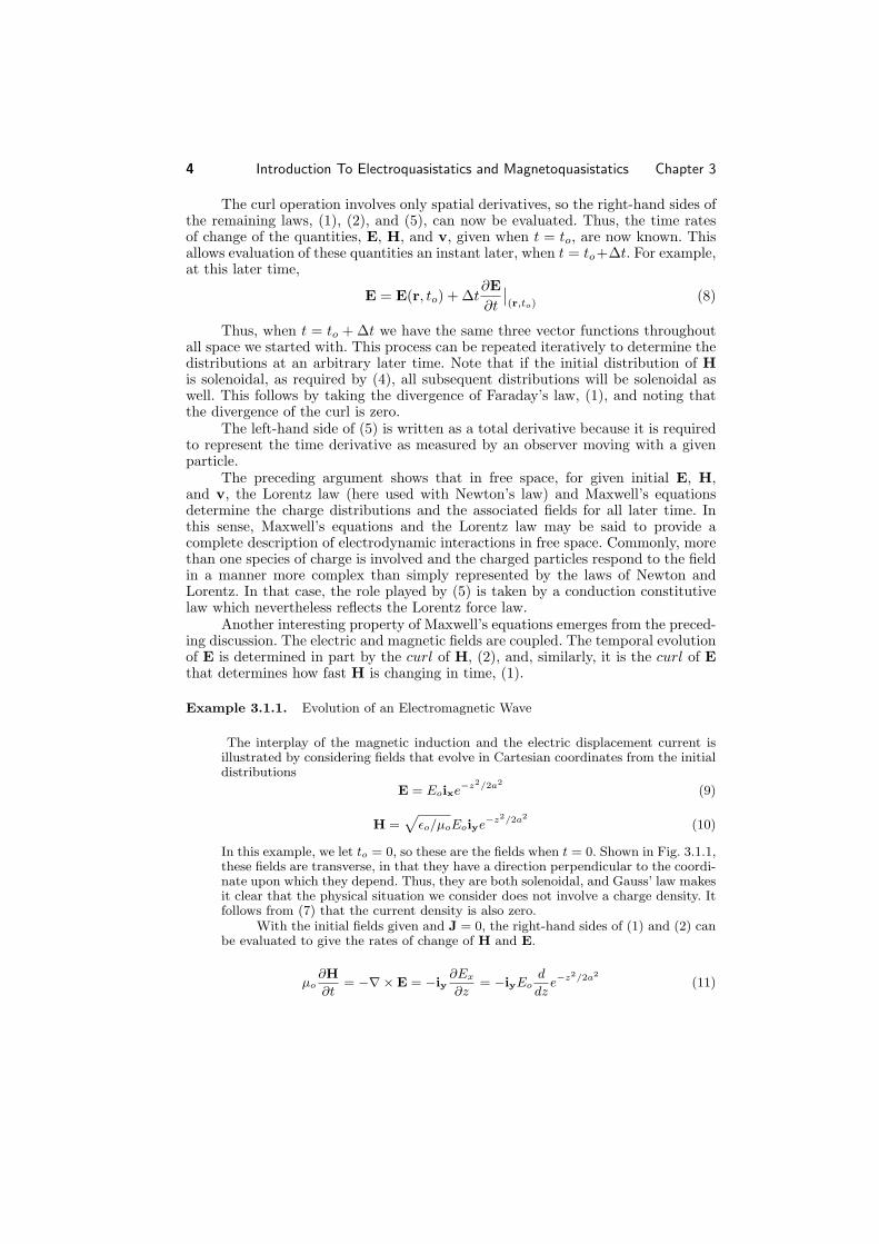
The interplay of the magnetic induction and the electric displacement current is illustrated by considering fields that evolve in Cartesian coordinates from the initial distributions

E = Eoixe−z 2/2a 2 (9)

2/2a 2 H = �

�o/µoEoiye−z (10)

In this example, we let to = 0, so these are the fields when t = 0. Shown in Fig. 3.1.1, these fields are transverse, in that they have a direction perpendicular to the coordinate upon which they depend. Thus, they are both solenoidal, and Gauss’ law makes it clear that the physical situation we consider does not involve a charge density. It follows from (7) that the current density is also zero.

With the initial fields given and J = 0, the righthand sides of (1) and (2) can be evaluated to give the rates of change of H and E.

∂H ∂Ex d 2/2a 2 µo ∂t

= −� × E = −iy ∂z

= −iyEo dz

e−z (11)

5 Sec. 3.1 Temporal Evolution of World

Fig. 3.1.1 A schematic representation of the E and H fields of Example 3.2.1. The distributions move to the right with the speed of light, c.

∂E d 2/2a 2 �o ∂t

= �× H = −ix�

�o/µoEo dz

e−z (12)

It follows from (11), Faraday’s law, that when t = Δt,

H = iy�

�o/µoEo

�e−z 2/2a 2 − cΔt

d e−z 2/2a 2

� (13)

dz

where c = 1/√

�oµo, and from (12), Ampere’s law, that the electric field is

E = Eoix�e−z 2/2a 2 − cΔt

d e−z 2/2a 2

� (14)

dz

When t = Δt, the E and H fields are equal to the original Gaussian distribution minus cΔt times the spatial derivatives of these Gaussians. But these represent the original Gaussians shifted by cΔt in the +z direction. Indeed, witness the relation applicable to any function f(z).

df f(z − Δz) = f(z)− Δz . (15)

dz

On the left, f(z − Δz) is the function f(z) shifted by Δz. The Taylor expansion on the right takes the same form as the fields when t = Δt, (13) and (14). Thus, within Δt, the E and H field distributions have shifted by cΔt in the +z direction. Iteration of this process shows that the field distributions shown in Fig. 3.1.1 travel in the +z direction without change of shape at the speed c, the speed of light.

c = √�

1

oµo = 3× 108 m/sec∼

(16)

Note that the derivation would not have changed if we had substituted for the initial Gaussian functions any other continuous functions f(z).

In retrospect, it should be recognized that the initial conditions were premeditated so that they would result in a single wave propagating in the +z direction. Also, the method of solution was really not numerical. If we were interested in pursuing the numerical approach, care would have to be taken to avoid the accumulation of errors.


The above example illustrated that the electromagnetic wave is caused by the interplay of the magnetic induction and the displacement current, the terms on the left in (1) and (2). Through Faraday’s law, (1), the curl of an initial E implies that an instant later, the initial H is altered. Similarly, Ampere’s law requires that the curl of an initial H leads to a change in E. In turn, the curls of the altered E and H imply further changes in H and E, respectively.

There are two main points in this section. First, Maxwell’s equations, augmented by laws describing the interaction of the fields with the sources, are sufficient to describe the evolution of electromagnetic fields.

Second, in regions well removed from materials, electromagnetic fields evolve as electromagnetic waves. Typically, the time required for fields to propagate from one region to another, say over a distance L, is

L τem = (17)

c

where c is the velocity of light. The origin of these waves is the coupling between the laws of Faraday and Ampere afforded by the magnetic induction and the displacement current. If either one or the other of these terms is neglected, so too is any electromagnetic wave effect.

3.2 QUASISTATIC LAWS

The quasistatic laws are obtained from Maxwell’s equations by neglecting either the magnetic induction or the electric displacement current.

ELECTROQUASTATIC MAGNETOQUASISTATIC

� × E = − ∂µoH

∂t � 0 (1a) � × E = −

∂µoH

∂t (1b)

� × H = ∂�oE

∂t + J (2a) � × H =

∂�oE

∂t + J � J (2b)

� · �oE = ρ (3a) � · �oE = ρ (3b)

� · µoH = 0 (4a) � · µoH = 0 (4b)

7 Sec. 3.2 Quasistatic Laws

The electromagnetic waves that result from the coupling of the magnetic induction and the displacement current are therefore neglected in either set of quasistatic laws. Before considering order of magnitude arguments in support of these approximate laws, we recognize their differing orders of importance.

In Chaps. 4 and 8 it will be shown that if the curl and divergence of a vector are specified, then that vector is determined.

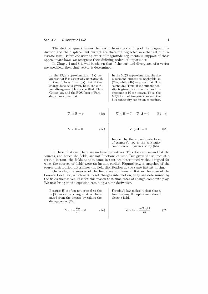
In the EQS approximation, (1a) requires that E is essentially irrotational. It then follows from (3a) that if the charge density is given, both the curl and divergence of E are specified. Thus, Gauss’ law and the EQS form of Faraday’s law come first.

� · �oE = ρ (5a)

�× E = 0 (6a)

In the MQS approximation, the displacement current is negligible in (2b), while (4b) requires that H is solenoidal. Thus, if the current density is given, both the curl and divergence of H are known. Thus, the MQS form of Ampere’s law and the flux continuity condition come first.

�× H = J; � · J = 0 (5b− c)

� · µoH = 0 (6b)

Implied by the approximate form of Ampere’s law is the continuity condition of J, given also by (5b).

In these relations, there are no time derivatives. This does not mean that the sources, and hence the fields, are not functions of time. But given the sources at a certain instant, the fields at that same instant are determined without regard for what the sources of fields were an instant earlier. Figuratively, a snapshot of the source distribution determines the field distribution at the same instant in time.

Generally, the sources of the fields are not known. Rather, because of the Lorentz force law, which acts to set charges into motion, they are determined by the fields themselves. It is for this reason that time rates of change come into play. We now bring in the equation retaining a time derivative.

Because H is often not crucial to the EQS motion of charges, it is eliminated from the picture by taking the divergence of (2a).

∂ρ

Faraday’s law makes it clear that a time varying H implies an induced electric field.

� · J + ∂t

= 0 (7a) = −∂µoH

(7b)�× E ∂t


In the EQS approximation, H is usually a “leftover” quantity. In any case, once E and J are determined, H can be found by solving (2a) and (4a).

∂�oE �× H = ∂t

+ J (8a)

� · µoH = 0 (9a)

In the MQS approximation, the charge density is a “leftover” quantity, which can be found by applying Gauss’ law, (3b), to the previously determined electric field intensity.

� · �oE = ρ (8b)

In the EQS approximation, it is clear that with E and J determined from the “zero order” laws (5a)–(7a), the curl and divergence of H are known [(8a) and (9a)]. Thus, H can be found in an “after the fact” way. Perhaps not so obvious is the fact that in the MQS approximation, the divergence and curl of E are also determined without regard for ρ. The curl of E follows from Faraday’s law, (7b), while the divergence is often specified by combining a conduction constitutive law with the continuity condition on J, (5b).

The differential quasistatic laws are summarized in Table 3.6.1 at the end of the chapter. Because there is a direct correspondence between terms in the differential and integral laws, the quasistatic integral laws are as summarized in Table 3.6.2. The conditions under which these quasistatic approximations are valid are examined in the next section.

3.3 CONDITIONS FOR FIELDS TO BE QUASISTATIC

An appreciation for the quasistatic approximations will come with a consideration of many case studies. Justification of one or the other of the approximations hinges on using the quasistatic fields to estimate the “error” fields, which are then hopefully found to be small compared to the original quasistatic fields.

In developing any mathematical “theory” for the description of some part of the physical world, approximations are made. Conclusions based on this “theory” should indeed be made with a concern for implicit approximations made out of ignorance or through oversight. But in making quasistatic approximations, we are fortunate in having available the “exact” laws. These can always be used to test the validity of a tentative approximation.

Provided that the system of interest has dimensions that are all within a factor of two or so of each other, order of magnitude arguments easily illustrate how the error fields are related to the quasistatic fields. The examples shown in Fig. 3.3.1 are not to be considered in detail, but rather should be regarded as prototypes. The candidate for the EQS approximation in part (a) consists of metal spheres that are insulated from each other and driven by a source of EMF. In the case of part (b), which is proposed for the MQS approximation, a current source drives a current around a oneturn loop. The dimensions are “on the same order” if the diameter of one of the spheres, is within a factor of two or so of the spacing between spheres

9 Sec. 3.3 Conditions for Quasistatics

Fig. 3.3.1 Prototype systems involving one typical length. (a) EQS system in which source of EMF drives a pair of perfectly conducting spheres having radius and spacing on the order of L. (b) MQS system consisting of perfectly conducting loop driven by current source. The radius of the loop and diameter of its crosssection are on the order of L.

and if the diameter of the conductor forming the loop is within a similar factor of the diameter of the loop.

If the system is pictured as made up of “perfect conductors” and “perfect insulators,” the decision as to whether a quasistatic field ought to be classified as EQS or MQS can be made by a simple rule of thumb: Lower the time rate of change (frequency) of the driving source so that the fields become static. If the magnetic field vanishes in this limit, then the field is EQS; if the electric field vanishes the field is MQS. In reality, materials are not “perfect,” neither perfect conductors nor perfect insulators. Therefore, the usefulness of this rule depends on understanding under what circumstances materials tend to behave as “perfect” conductors, and insulators. Fortunately, nature provides us with metals that are extremely good conductors– and with gases, liquids, and solids that are very good insulators– so that this rule is a good intuitive starting point. Chapters 7, 10, and 15 will provide a more mature view of how to classify quasistatic systems.

The quasistatic laws are now used in the order summarized by (3.2.5)(3.2.9) to estimate the field magnitudes. With only one typical length scale L, we can approximate spatial derivatives that make up the curl and divergence operators by 1/L.

ELECTROQUASISTATIC MAGNETOQUASISTATIC

Thus, it follows from Gauss’ law, (3.2.5a), that typical values of E and ρ are related by

�oE ρL = ρ E = (1a)

L ⇒

�o

Thus, it follows from Ampere’s law, (3.2.5b), that typical values of H and J are related by

H = J H = JL (1b)

L ⇒

As suggested by the integral forms of the laws so far used, these fields and their sources are sketched in Fig. 3.3.1. The EQS laws will predict E lines that originate on the positive charges on one electrode and terminate on the negative charges on the other. The MQS laws will predict lines of H that close around the circulating current.

If the excitation were sinusoidal in time, the characteristic time τ for the


sinusoidal steady state response would be the reciprocal of the angular frequency ω. In any case, if the excitations are time varying, with a characteristic time τ , then

the time varying charge implies a current, and this in turn induces an H. We could compute the current in the conductors from charge conservation, (3.2.7a), but because we are interested in the induced H, we use Ampere’s law, (3.2.8a), evaluated in the free space region. The electric field is replaced in favor of the charge density in this expression using (1a).

H �oE =

L

H =

τ ⇒

�oEL =

L2ρ (2a)

τ τ

the timevarying current implies an H that is timevarying. In accordance with Faraday’s law, (3.2.7b), the result is an induced E. The magnetic field intensity is replaced by J in this expression by making use of (1b).

E =

µoH

L

E =

τ ⇒

µoHL =

µoJL2 (2b)

τ τ

What errors are committed by ignoring the magnetic induction and displacement current terms in the respective EQS and MQS laws?

The electric field induced by the quasistatic magnetic field is estimated by using the H field from (2a) to estimate the contribution of the induction term in Faraday’s law. That is, the term originally neglected in (3.2.1a) is now estimated, and from this a curl of an error field evaluated.

Eerror =

µoρL2

L

Eerror =

τ2

µoρL3

τ2

⇒ (3a)

The magnetic field induced by the displacement current represents an error field. It can be estimated from Ampere’s law, by using (2b) to evaluate the displacement current that was originally neglected in (3.2.2b).

Herror =

�oµoJL2

L

Herror =

τ2

�oµoJL3

τ2

⇒ (3b)

Sec. 3.3 Conditions for Quasistatics 11

It follows from this expression and (1a) that the ratio of the error field to the quasistatic field is

Eerror

E =

µo�oL2

τ2 (4a)

It then follows from this and (1b) that the ratio of the error field to the quasistatic field is

Herror �oµoL2

= (4b)H τ2

For the approximations to be justified, these error fields must be small compared to the quasistatic fields. Note that whether (4a) is used to represent the EQS system or (4b) is used for the MQS system, the conditions on the spatial scale L and time τ (perhaps the reciprocal frequency) are the same.

Both the EQS and MQS approximations are predicated on having sufficiently slow time variations (low frequencies) and sufficiently small dimensions so that

µo�oL2 L

τ2 � 1 � τ (5)⇒

c

where c = 1/√

�oµo. The ratio L/c is the time required for an electromagnetic wave to propagate at the velocity c over a length L characterizing the system. Thus, either of the quasistatic approximations is valid if an electromagnetic wave can propagate a characteristic length of the system in a time that is short compared to times τ of interest.

If the conditions that must be fulfilled in order to justify the quasistatic approximations are the same, how do we know which approximation to use? For systems modeled by free space and perfect conductors, such as we have considered here, the answer comes from considering the fields that are retained in the static limit (infinite τ or zero frequency ω).

Recapitulating the rule expressed earlier, consider the pair of spheres shown in Fig. 3.3.1a. Excited by a constant source of EMF, they are charged, and the charges give rise to an electric field. But in this static limit, there is no current and hence no magnetic field. Thus, the static system is dominated by the electric field, and it is natural to represent it as being EQS even if the excitation is timevarying.

Excited by a dc source, the circulating current in Fig. 3.3.1b gives rise to a magnetic field, but there are no charges with attendant electric fields. This time it is natural to use the MQS approximation when the excitation is time varying.

Example 3.3.1. Estimate of Error Introduced by Electroquasistatic Approximation

Consider a simple structure fed by a set of idealized sources of EMF as shown in Fig. 3.3.2. Two circular metal disks, of radius b, are spaced a distance d apart. A distribution of EMF generators is connected between the rims of the plates so that the complete system, plates and sources, is cylindrically symmetric. With the understanding that in subsequent chapters we will be examining the underlying physical processes, for now we assume that, because the plates are highly conducting, E must be perpendicular to their surfaces.

The electroquasistatic field laws are represented by (3.2.5a) and (3.2.6a). A simple solution for the electric field between the plates is

E = E iz ≡ Eoiz (6)

d


Fig. 3.3.2 Plane parallel electrodes having no resistance, driven at their outer edges by a distribution of sources of EMF.

Fig. 3.3.3 Parallel plates of Fig. 3.3.2, showing volume containing lower plate and radial surface current density at its periphery.

where the sign definition of the EMF, E , is as indicated in Fig. 3.3.2. The field of (6) satisfies (3.2.5a) and (3.2.6a) in the region between the plates because it is both irrotational and solenoidal (no charge is assumed to exist in the region between the plates). Further, the field has no component tangential to the plates which is consistent with the assumption of plates with no resistance. Finally, Gauss’ jump condition, (1.3.17), can be used to find the surface charges on the top and bottom plates. Because the fields above the upper plate and below the lower plate are assumed to be zero, the surface charge densities on the bottom of the top plate and on the top of the bottom plate are

Ez(z = d) = Eo; z = d� −�o −�oσs = (7)

�oEz(z = 0) = �oEo; z = 0

There remains the question of how the electric field in the neighborhood of the distributed source of EMF is constrained. We assume here that these sources are connected in such a way that they make the field uniform right out to the outer edges of the plates. Thus, it is consistent to have a field that is uniform throughout the entire region between the plates. Note that the surface charge density on the plates is also uniform out to r = b. At this point, (3.2.5a) and (3.2.6a) are satisfied between and on the plates.

In the EQS order of laws, conservation of charge comes next. Rather than using the differential form, (3.2.7a), we use the integral form, (1.5.2). The volume V is a cylinder of circular crosssection enclosing the lower plate, as shown in Fig. 3.3.3. Because the radial surface current density in the plate is independent of φ, integration of J da on the enclosing surface amounts to multiplying Kr by the circumference,· while the integration over the volume is carried out by multiplying σs by the surface area, because the surface charge density is uniform. Thus,

Kr2πb + πb2�o dEo

= 0 ⇒ Kr

�� = − b�

2 o dEo

(8)dt r=b dt

In order to find the magnetic field, we make use of the “secondary” EQS laws, (3.2.8a) and (3.2.9a). Ampere’s law in integral form, (1.4.1), is convenient for the present case of high symmetry. The displacement current is z directed, so the

�

Sec. 3.3 Conditions for Quasistatics 13

Fig. 3.3.4 Crosssection of system shown in Fig. 3.3.2 showing surface and contour used in evaluating correction E field.

surface S is taken as being in the free space region between the plates and having a zdirected normal. � �

∂�oE H ds = izda (9)·

∂t ·

C S

The symmetry of structure and source suggests that H must be φ independent. A centered circular contour of radius r, as in Fig. 3.3.2, with z in the range 0 < z < d, gives

dEo 2 r dEoHφ2πr = �o πr Hφ = �o (10)

dt ⇒

2 dt

Thus, for this specific configuration, we are at a point in the analysis represented by (2a) in the order of magnitude arguments.

Consider now “higher order” fields and specifically the error committed by neglecting the magnetic induction in the EQS approximation. The correct statement of Faraday’s law is (3.2.1a), with the magnetic induction retained. Now that the quasistatic H has been determined, we are in a position to compute the curl of E that it generates.

Again, for this highly symmetric configuration, it is best to use the integral law. Because H is φ directed, the surface is chosen to have its normal in the φ direction, as shown in Fig. 3.3.4. Thus, Faraday’s integral law (1.6.1) becomes

� � ∂µoHφ

E ds = iφ da (11)· − ∂t

· C S

We use the contour shown in Fig. 3.3.4 and assume that the E induced by the magnetic induction is independent of z. Because the tangential E field is zero on the plates, the only contributions to the line integral on the left in (11) come from the vertical legs of the contour. The surface integral on the right is evaluated using (10).

b µo�od

� d2Eo

[Ez(b)− Ez(r)]d = r�dr� 2 dt2

r (12) µo�od 2 2 d2Eo

= (b − r )4 dt2

The field at the outer edge is constrained by the EMF sources to be Eo, and so it follows from (12) that to this order of approximation the electric field is

Ez = Eo + �oµo d

2Eo (r 2 − b2) (13)

4 dt2

We have found that the electric field at r = b differs from the field at the edge. How big is the difference? This depends on the time rate of variation of the electric field.


For purposes of illustration, assume that the electric field is sinusoidally varying with time.

Eo(t) = A cos ωt (14)

Thus, the time characterizing the dynamics is 1/ω. Introducing this expression into (13), and calling the second term the “error

field,” the ratio of the error field and the field at the rim, where r = b, is

|Eerror | =

1 ω2�oµo(b

2 − r 2) (15)Eo 4

The error field will be negligible compared to the quasistatic field if

ω2�oµob2

� 1 (16)4

for all r between the plates. In terms of the free space wavelength λ, defined as the distance an electromagnetic wave propagates at the velocity c = 1/

√�oµo in one

cycle 2π/ω

λ 2π = : c ≡ 1/

√µo�o (17)

c ω

(16) becomes

b2 � (λ/π)2 (18)

In free space and at a frequency of 1 MHz, the wavelength is 300 meters. Hence, if we build a circular disk capacitor and excite it at a frequency of 1 MHz, then the quasistatic laws will give a good approximation to the actual field as long as the radius of the disk is much less than 300 meters.

The correction field for a MQS system is found by following steps that are analogous to those used in the previous example. Once the magnetic and electric fields have been determined using the MQS laws, the error magnetic field induced by the displacement current can be found.

3.4 QUASISTATIC SYSTEMS1

Whether we ignore the magnetic induction and use the EQS approximation, or neglect the displacement current and make a MQS approximation, times of interest τ must be long compared to the time τem required for an electromagnetic wave to propagate at the velocity c over the largest length L of the system.

L τem = � τ (1)

c

1 This section makes use of the integral laws at a level somewhat more advanced than necessary in preparation for the next chapter. It can be skipped without loss of continuity.

Sec. 3.4 Quasistatic Systems 15

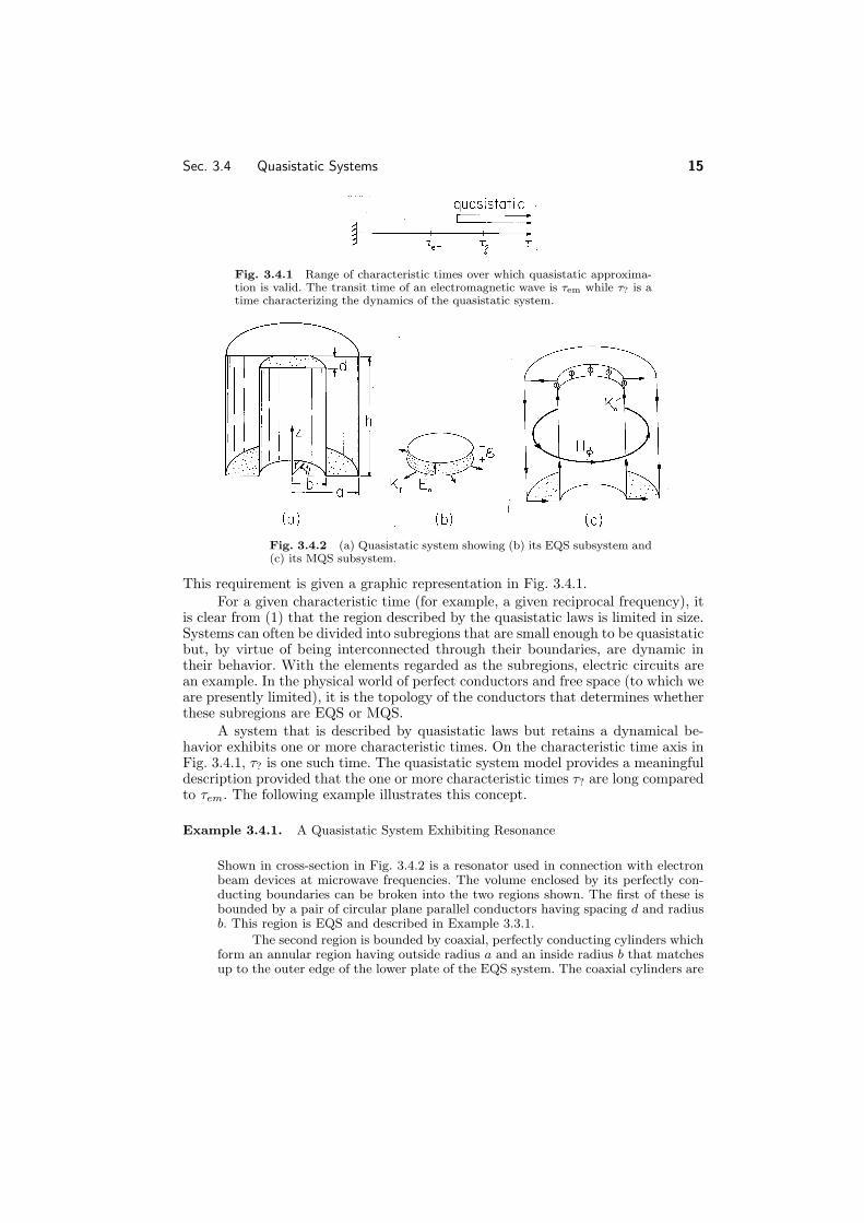
Fig. 3.4.1 Range of characteristic times over which quasistatic approximation is valid. The transit time of an electromagnetic wave is τem while τ? is a time characterizing the dynamics of the quasistatic system.

Fig. 3.4.2 (a) Quasistatic system showing (b) its EQS subsystem and (c) its MQS subsystem.

This requirement is given a graphic representation in Fig. 3.4.1. For a given characteristic time (for example, a given reciprocal frequency), it

is clear from (1) that the region described by the quasistatic laws is limited in size. Systems can often be divided into subregions that are small enough to be quasistatic but, by virtue of being interconnected through their boundaries, are dynamic in their behavior. With the elements regarded as the subregions, electric circuits are an example. In the physical world of perfect conductors and free space (to which we are presently limited), it is the topology of the conductors that determines whether these subregions are EQS or MQS.

A system that is described by quasistatic laws but retains a dynamical behavior exhibits one or more characteristic times. On the characteristic time axis in Fig. 3.4.1, τ? is one such time. The quasistatic system model provides a meaningful description provided that the one or more characteristic times τ? are long compared to τem. The following example illustrates this concept.

Example 3.4.1. A Quasistatic System Exhibiting Resonance

Shown in crosssection in Fig. 3.4.2 is a resonator used in connection with electron beam devices at microwave frequencies. The volume enclosed by its perfectly conducting boundaries can be broken into the two regions shown. The first of these is bounded by a pair of circular plane parallel conductors having spacing d and radius b. This region is EQS and described in Example 3.3.1.

The second region is bounded by coaxial, perfectly conducting cylinders which form an annular region having outside radius a and an inside radius b that matches up to the outer edge of the lower plate of the EQS system. The coaxial cylinders are

� �


Fig. 3.4.3 Surface S and contour C for evaluating Hfield using Ampere’s law.

shorted by a perfectly conducting plate at the bottom, where z = 0. A similar plate at the top, where z = h, connects the outer cylinder to the outer edge of the upper plate in the EQS subregion.

For the moment, the subsystems are isolated from each other by driving the MQS system with a current source Ko (amps/meter) distributed around the periphery of the gap between conductors. This gives rise to axial surface current densities of Ko and −Ko(b/a) on the inner and outer cylindrical conductors and radial surface current densities contributing to J da in the upper and lower plates, respectively. · (Note that these satisfy the MQS current continuity requirement.)

Because of the symmetry, the magnetic field can be determined by using the integral MQS form of Ampere’s law. So that there is a contribution to the integration of J da, a surface is selected with a normal in the axial direction. This surface is· enclosed by a circular contour having the radius r, as shown in Fig. 3.4.3. Because of the axial symmetry, Hφ is independent of φ, and the integrations on S and C amount to multiplications.

H ds = J izda 2πrHφ = 2πbKo (2)· · ⇒C S

Thus, in the annulus, b

Hφ = Ko (3) r

In the regions outside the annulus, H is zero. Note that this is consistent with Ampere’s jump condition, (1.4.16), evaluated on any of the boundaries using the already determined surface current densities. Also, we will find in Chap. 10 that there can be no timevarying magnetic flux density normal to a perfectly conducting boundary. The magnetic field given in (3) satisfies this condition as well.

In the hierarchy of MQS laws, we have now satisfied (3.2.5b) and (3.2.6b) and come next to Faraday’s law, (3.2.7b). For the present purposes, we are not interested in the details of the distribution of electric field. Rather, we use the integral form of Faraday’s law, (1.6.1), integrated on the surface S shown in Fig. 3.4.4. The integral of E ds along the perfect conductor vanishes and we are left with ·

b� dλf Eab = E ds = (4)· dt

a

where the EMF across the gap is as defined by (1.6.2), and the flux linked by C is consistent with (1.6.8).

λf = h

� a

µoHφdr = µobhKo

� a dr

= µohb ln� a�

Ko (5) r b

b b

.

Sec. 3.4 Quasistatic Systems 17

Fig. 3.4.4 Surface S and contour C used to determine EMF using Faraday’s law.

These last two expressions combine to give

Eab = µohb ln� a� dKo

(6)b dt

Just as this expression serves to relate the EMF and surface current density at the gap of the MQS system, (3.3.8) relates the gap variables defined in Fig. 3.4.2b for the EQS subsystem. The subsystems are now interconnected by replacing the distributed current source driving the MQS system with the peripheral surface current density of the EQS system.

Kr + Ko = 0 (7)

In addition, the EMF’s of the two subsystems are made to match where they join.

−E = Eab (8)

With (3.3.8) and (3.3.6), respectively, substituted for Kr and Eab, these expressions become two differential equations in the two variables Eo and Ko describing the complete system.

b�o dEo − 2

+ Ko = 0 (9)dt

−dEo = µobh ln� a� dKo

(10)b dt

Elimination of Ko between these expressions gives

d2Eo + ωo

2Eo = 0 (11)dt2

where ωo is defined as

ωo 2 =

�oµohb

22

d

ln�

ab

� (12)

and it follows that solutions are a linear combination of sin ωot and cos ωot. As might have been suspected from the outset, what we have found is a re

sponse to initial conditions that is oscillatory, with a natural frequency ωo. That is, the parallel plate capacitor that comprises the EQS subsystem, connected in parallel with the oneturn inductor that is the MQS subsystem, responds to initial values of Eo and Ko with an oscillation that at one instant has Eo at its peak magnitude and Ko = 0, and a quarter cycle later has Eo = 0 and Ko at its peak magnitude.


Fig. 3.4.5 In terms of characteristic time τ , the dynamic regime in which the system of Fig. 3.4.2 is quasistatic but capable of being in a state of resonance.

Remember that �oEo is the surface charge density on the lower plate in the EQS section. Thus, the oscillation is between the charges in the EQS subsystem and the currents in the MQS subsystem. The distribution of field sources in the system as a whole is determined by a dynamical interaction between the two subsystems.

If the system were driven by a current source having the frequency ω, it would display a resonance at the natural frequency ωo. Under what conditions can the system be in resonance and still be quasistatic? In this case, the characteristic time for the system dynamics is the reciprocal of the resonance frequency. The EQS subsystem is indeed EQS if b/c � τ , while the annular subsystem is MQS if h/c � τ . Thus, the resonance is correctly described by the quasistatic model if the times have the ordering shown in Fig. 3.4.5. Essentially, this is achieved by making the spacing d in the EQS section very small.

With the region of interest containing media, the appropriate quasistatic limit is often as much determined by the material properties as by the topology. In Chaps. 7 and 10, we will consider lossy materials where the distributions of field sources depend on the time rates of change and a given region can be EQS or MQS depending on the electrical conductivity. We return to the subject of quasistatics in Chaps. 12 and 14.

3.5 OVERVIEW OF APPLICATIONS

Electroquasistatics is the subject of Chaps. 4–7 and magnetoquasistatics the topic of Chaps. 8–10. Before embarking on these subjects, consider in this section some practical examples that fall in each category, and some that involve the electrodynamics of Chaps. 12–14.

Our starting point is at location A at the upper right in Fig. 3.5.1. With frequencies that range from 60400 MHz, television signals propagate from remote locations to our homes as electromagnetic waves. If the frequency is f , the field passes through one period in the time 1/f . Setting this equal to the transit time, (3.1.l7) gives an expression for the wavelength, the distance the wave travels during one cycle.

c =L ≡ λ

f

Thus, for channel 2 (60 MHz) the wavelength is about 5 m, while for channel 54 it is about 20 cm. The distance between antenna and receiver is many wavelengths, and hence the fields undergo many oscillations while traversing the space between the two. The dynamics is not quasistatic but rather intimately involves the electromagnetic wave represented by inset B and described in Sec. 3.1.

Sec. 3.5 Overview of Applications 19

Fig. 3.5.1 Quasistatic and electrodynamic fields in the physical world.

The field induces charges and currents in the antenna, and the resulting signals are conveyed to the TV set by a transmission line. At TV frequencies, the line is likely to be many wavelengths long. Hence, the fields surrounding the line are also not quasistatic. But the radial distributions of current in the elements of the antennas and in the wires of the transmission line are governed by magnetoquasistatic (MQS) laws. As suggested by inset C, the current density tends to concentrate


adjacent to the conductor surfaces and this skin effect is MQS. Inside the television set, in the transistors and picture tube that convert the

signal to an image and sound, electroquasistatic (EQS) processes abound. Included are dynamic effects in the transistors (E) that result from the time required for an electron or hole to migrate a finite distance through a semiconductor. Also included are the effects of inertia as the electrons are accelerated by the electric field in the picture tube (D). On the other hand, the speaker that transduces the electrical signals into sound is most likely MQS.

Electromagnetic fields are far closer to the viewer than the television set. As is obvious to those who have had an electrocardiogram, the heart (F) is the source of a pulsating current. Are the distributions of these currents and the associated fields described by the EQS or MQS approximation? On the largest scales of the body, we will find that it is MQS.

Of course, there are many other sources of electrical currents in the body. Nerve conduction and other electrical activity in the brain occur on much smaller length scales and can involve regions of much less conductivity. These cases can be EQS.

Electrical power systems provide diverse examples as well. The stepdown transformer on a pole outside the home (G) is MQS, with dynamical processes including eddy currents and hysteresis.

The energy in all these examples originates in the fuel burned in a power plant. Typically, a steam turbine drives a synchronous alternator (H). The fields within this generator of electrical power are MQS. However, most of the electronics in the control room (J) are described by the EQS approximation. In fact, much of the payoff in making computer components smaller is gained by having them remain EQS even as the bit rate is increased. The electrostatic precipitator (I), used to remove flyash from the combustion gases before they are vented from the stacks, seems to be an obvious candidate for the EQS approximation. Indeed, even though some modern precipitators use pulsed high voltage and all involve dynamic electrical discharges, they are governed by EQS laws.

The power transmission system is at high voltage and therefore might naturally be regarded as EQS. Certainly, specification of insulation performance (K) begins with EQS approximations. However, once electrical breakdown has occurred, enough current can be faulted to bring MQS considerations into play. Certainly, they are present in the operation of highpower switch gear. To be even a fraction of a wavelength at 60 Hz, a line must stretch the length of California. Thus, in so far as the power frequency fields are concerned, the system is quasistatic. But certain aspects of the power line itself are MQS, and others EQS, although when lightning strikes it is likely that neither approximation is appropriate.

Not all fields in our bodies are of physiological origin. The man standing under the power line (L) finds himself in both electric and magnetic fields. How is it that our bodies can shield themselves from the electric field while being essentially transparent to the magnetic field without having obvious effects on our hearts or nervous systems? We will find that currents are indeed induced in the body by both the electric and magnetic fields, and that this coupling is best understood in terms of the quasistatic fields. By contrast, because the wavelength of an electromagnetic wave at TV frequencies is on the order of the dimensions of the body, the currents induced in the person standing in front of the TV antenna at A are not quasistatic.

Sec. 3.6 Summary 21

As we make our way through the topics outlined in Fig. 3.5.1, these and other physical situations will be taken up by the examples.

3.6 SUMMARY

From a mathematical point of view, the summary of quasistatic laws given in Table 3.6.1 is an outline of the next seven chapters.

An excursion down the left column and then down the right column of the outline represented by Fig. 1.0.1 carries us down the corresponding columns of the table. Gauss’ law and the requirement that E be irrotational, (3.2.5a) and (3.2.6a), are the subjects of Chaps. 4–5. In Chaps. 6 and 7, two types of charge density are distinguished and used to represent the effects of macroscopic media on the electric field. In Chap. 6, where polarization charge is used to represent insulating media, charge is automatically conserved. But in Chap. 7, where unpaired charges are created through conduction processes, the charge conservation law, (3.2.7a), comes into play on the same footing as (3.2.5a) and (3.2.6a). In stages, starting in Chap. 4, the ability to predict selfconsistent distributions of E and ρ is achieved in this last EQS chapter.

Ampere’s law and magnetic flux continuity, (3.2.5b) and (3.2.6b), are featured in Chap. 8. First, the magnetic field is determined for a given distribution of current density. Because current distributions are often controlled by means of wires, it is easy to think of practical situations where the MQS source, the current density, is known at the outset. But even more, the first half of Chap. 7 was already devoted to determining distributions of “stationary” current densities. The MQS current density is always solenoidal, (3.2.5c), and the magnetic induction on the right in Faraday’s law, (3.2.7b), is sometimes negligible so that the electric field can be essentially irrotational. Thus, the first half of Chap. 7 actually starts the sequence of MQS topics. In the second half of Chap. 8, the magnetic field is determined for systems of perfect conductors, where the source distribution is not known until the fields meet certain boundary conditions. The situation is analogous to that for EQS systems in Chap. 5. Chapters 9 and 10 distinguish between effects of magnetization and conduction currents caused by macroscopic media. It is in Chap. 10 that Faraday’s law, (3.2.7b), comes into play in a field theoretical sense. Again, in stages, in Chaps. 8–10, we attain the ability to describe a selfconsistent field and source evolution, this time of H and its sources, J.

The quasistatic approximations and ordering of laws can just as well be stated in terms of the integral laws. Thus, the differential laws summarized in Table 3.6.1 have the integral law counterparts listed in Table 3.6.2.


TABLE 3.6.1

SUMMARY OF QUASISTATIC DIFFERENTIAL

LAWS IN FREE SPACE

ELECTROQUASISTATIC MAGNETOQUASISTATIC Reference Eq.

� · �oE = ρ

� × E = 0

� · J + ∂ρ

∂t = 0

� × H = J; � · J = 0

� · µoH = 0

� × E = −∂µoH

∂t

(3.2.5)

(3.2.6)

(3.2.7)

Secondary

� × H = J + ∂�oE

∂t

� · µoH = 0

� · �oE = ρ (3.2.8)

(3.2.9)

TABLE 3.6.2

SUMMARY OF QUASISTATIC INTEGRAL

LAWS IN FREE SPACE

(a)

ELECTROQUASISTATIC

(b)

MAGNETOQUASISTATIC Eq.

�S

�oE · da = �

V ρdv

�C

E · ds = 0

�S J · da + d

dt

�V

ρdV = 0

�C

H · ds = �

S J · da;

�S J · da = 0

�S

µoH · da = 0

�C

E · ds = − d dt

�S

µ0H · da

(1)

(2)

(3)

Secondary

�C

H · ds = �

S J · da + d

dt

�S

�oE · da �

S µoH · da = 0

�S

�oE · da = �

V ρdv (4)

(5)

23 Sec. 3.2 Problems

P R O B L E M S

3.1 Temporal Evolution of World Governed by Laws of Maxwell, Lorentz, and Newton

3.1.1 In Example 3.1.1, it was shown that solutions to Maxwell’s equations can take the form E = Ex(z − ct)ix and H = Hy(z − ct)iy in a region where J = 0 and ρ = 0.

(a) Given E and H by (9) and (10) when t = 0, what are these fields for t > 0?

(b) By substituting these expressions into (1)–(4), show that they are exact solutions to Maxwell’s equations.

(c) Show that for an observer at z = ct+ constant, these fields are constant.

3.1.2∗ Show that in a region where J = 0 and ρ = 0 and a solution to Maxwell’s equations E(r, t) and H(r, t) has been obtained, a second solution is obtained by replacing H by −E, E by H, � by µ and µ by �.

3.1.3 In Prob. 3.1.1, the initial conditions given by (9) and (10) were arranged so that for t > 0, the fields took the form of a wave traveling in the +z direction.

(a) How would you alter the magnetic field intensity, (10), so that the ensuing field took the form of a wave traveling in the −z direction?

(b) What would you make H, so that the result was a pair of electric field intensity waves having the same shape, one traveling in the +z direction and the other traveling in the −z direction?

3.1.4 When t = 0, E = Eoiz cos βx, where Eo and β are given constants. When t = 0, what must H be to result in E = Eoiz cos β(x − ct) for t > 0.

3.2 Quasistatic Laws

3.2.1 In Sec. 13.1, we will find that fields of the type considered in Example 3.1.1 can exist between the plane parallel plates of Fig. P3.2.1. In the particular case where the plates are “open” at the right, where z = 0, it will be found that between the plates these fields are

cos βz E = Eo cos ωtix (a)

cos βl

� �o sin βz

H = Eo sin ωtiy (b) µo cos βl


Fig. P3.2.1

Fig. P3.2.2

where β = ω√

µo�o and Eo is a constant established by the voltage source at the left.

(a) By substitution, show that in the free space region between the plates (where J = 0 and ρ = 0), (a) and (b) are exact solutions to Maxwell’s equations.

(b) Use trigonometric identities to show that these fields can be decomposed into sums of waves traveling in the ±z directions. For example, Ex = E+(z − ct) + E (z + ct), where c is defined by (3.1.16) and E are functions of z � ct

−, respectively.

±

(c) Show that if βl � 1, the time l/c required for an electromagnetic wave to traverse the length of the electrodes is short compared to the time τ ≡ 1/ω within which the driving voltage is changing.

(d) Show that in the limit where this is true, (a) and (b) become

E Eo cos ωtix (c)→

H Eo�oωz sin ωtiy (d)→

so that the electric field between the plates is uniform. (e) With the frequency low enough so that (c) and (d) are good approx

imations to the fields, do these solutions satisfy the EQS or MQS laws?

3.2.2 In Sec. 13.1, it will be shown that the electric and magnetic fields between the plane parallel plates of Fig. P3.2.2 are

� µo sin βz

E = Ho sin ωtix (a)�o cos βl


cos βz H = Ho cos ωtiy (b)

cos βl

where β = ω√

µo�o and Ho is a constant determined by the current source at the left. Note that because the plates are “shorted” at z = 0, the electric field intensity given by (a) is zero there.

(a) Show that (a) and (b) are exact solutions to Maxwell’s equations in the region between the plates where J = 0 and ρ = 0.

(b) Use trigonometric identities to show that these fields take the form of waves traveling in the ±z directions with the velocity c defined by (3.1.16).

(c) Show that the condition βl � 1 is equivalent to the condition that the wave transit time l/c is short compared to τ ≡ 1/ω.

(d) For the frequency ω low enough so that the conditions of part (c) are satisfied, give approximate expressions for E and H. Describe the distribution of H between the plates.

(e) Are these approximate fields governed by the EQS or the MQS laws?

3.3 Conditions for Fields to be Quasistatic

3.3.1 Rather than being in the circular geometry of Example 3.3.1, the configuration considered here and shown in Fig. P3.3.1 consists of plane parallel rectangular electrodes of (infinite) width w in the y direction, spacing d in the x direction and length 2l in the z direction. The region between these electrodes is free space. Voltage sources constrain the integral of E between the electrode edges to be the same functions of time.

� d

v = Ex(z = ±l)dx (a) 0

(a) Assume that the voltage sources are varying so slowly that the electric field is essentially static (irrotational). Determine the electric field between the electrodes in terms of v and the dimensions. What is the surface charge density on the inside surfaces of the electrodes? (These steps are very similar to those in Example 3.3.1.)

(b) Use conservation of charge to determine the surface current density Kz on the electrodes.

(c) Now use Ampere’s integral law and symmetry arguments to find H. With this field between the plates, use Ampere’s continuity condition, (1.4.16), to find K in the plates and show that it is consistent with the result of part (b).

(d) Because of the H found in part (c), E is not irrotational. Return to the integral form of Faraday’s law to find a corrected electric field intensity, using the magnetic field of part (c). [Note that the electric field found in part (a) already satisfies the conditions imposed by the voltage sources.]

Cite as: Markus Zahn, course materials for 6.641 Electromagnetic Fields, Forces, and Motion, Spring 2005. MIT OpenCourseWare (http://ocw.mit.edu/), Massachusetts Institute of Technology. Downloaded on [DD Month YYYY].


Fig. P3.3.1

(e) If the driving voltage takes the form v = vo cos ωt, determine the ratio of the correction (error) field to the quasistatic field of part (a).

3.3.2 The configuration shown in Fig. P3.3.2 is similar to that for Prob. 3.3.1 except that the sources distributed along the left and right edges are current rather than voltage sources and are of opposite rather than the same polarity. Thus, with the current sources varying slowly, a (zindependent) surface current density K(t) circulates around a loop consisting of the sources and the electrodes. The roles of E and H are the reverse of what they were in Example 3.3.1 or Prob. 3.3.1. Because the electrodes are pictured as having no resistance, the lowfrequency electric field is zero while, even if the excitations are constant in time, there is an H. The following steps answer the question, Under what circumstances is the electric displacement current negligible compared to the magnetic induction?

(a) Determine H in the region between the electrodes in a manner consistent with there being no H outside. (Ampere’s continuity condition relates H to K at the electrodes. Like the E field in Example 3.3.1 or Prob. 3.3.1, the H is extremely simple.)

(b) Use the integral form of Faraday’s law to determine E between the electrodes. Note that symmetry requires that this field be zero where z = 0.

(c) Because of this timevarying E, there is a displacement current density between the electrodes in the x direction. Use Ampere’s integral law to find the correction (error) H. Note that the quasistatic field already meets the conditions imposed by the current sources where z = ±l.

(d) Given that the driving currents are sinusoidal with angular frequency ω, determine the ratio of the “error” of H to the MQS field of part (a).

3.4 Quasistatic Systems

Cite as: Markus Zahn, course materials for 6.641 Electromagnetic Fields, Forces, and Motion, Spring 2005. MIT OpenCourseWare (http://ocw.mit.edu/), Massachusetts Institute of Technology. Downloaded on [DD Month YYYY].


Fig. P3.3.2

3.4.1 The configuration shown in cutaway view in Fig. P3.4.1 is essentially the outer region of the system shown in Fig. 3.4.2. The object here is to determine the error associated with neglecting the displacement current density in this outer region. In this problem, the region of interest is pictured as bounded on three sides by material having no resistance, and on the fourth side by a distributed current source. The latter imposes a surface current density Ko in the z direction at the radius r = b. This current passes radially outward through a plate in the z = h plane, axially downward in another conductor at the radius r = a, and radially inward in the plate at z = 0.

(a) Use the MQS form of Ampere’s integral law to determine H inside the “donut”shaped region. This field should be expressed in terms of Ko. (Hint: This step is essentially the same as for Example 3.4.1.)

(b) There is no H outside the structure. The interior field is terminated on the boundaries by a surface current density in accordance with Ampere’s continuity condition. What is K on each of the boundaries?

(c) In general, the driving current is time varying, so Faraday’s law requires that there be an electric field. Use the integral form of this law and the contour C and surface S shown in Fig. P3.4.2 to determine E. Assume that E tangential to the zeroresistance boundaries is zero. Also, assume that E is z directed and independent of z.

(d) Now determine the error in the MQS H by using Ampere’s integral law. This time the displacement current density is not approximated as zero but rather as implied by the E found in part (c). Note that the MQS H field already satisfies the condition imposed by the current source at r = b.

(e) With Ko = Kp cos ωt, write the condition for the error field to be small compared to the MQS field in terms of ω, c, and l.


Fig. P3.4.1

Fig. P3.4.2

electromagnetic fields and energy - mit … · haus, hermann a., and james r. melcher,...

Documents