electromagnetic vector-sensor array … · a three-dimensional (3-d) array of identically oriented...

Progress In Electromagnetics Research B, Vol. 39, 281–299, 2012

ELECTROMAGNETIC VECTOR-SENSOR ARRAY PRO-CESSING FOR DISTRIBUTED SOURCE LOCALIZATION

X. M. Shi* and Z. W. Liu

School of Information and Electronics, Beijing Institute of Technology,Beijing 100081, China

Abstract—We consider the problem of direction-of-arrival (DOA)estimation for distributed signals with electromagnetic vector sensors,of which each provides measurements of the complete electric andmagnetic fields induced by electromagnetic (EM) signals. In thispaper, we consider situations where the sources are distributed notonly in space with a deterministic angular signal density, but also inpolarization with partially polarized components. A distributed signalsgeneral model with electromagnetic vector-sensor array (EMVS-DIS)is established with some reasonable assumptions. Based on the EMVS-DIS model, the minimum-variance distortionless response (MVDR)estimators for distributed source DOA are derived. MVDR estimatorsdo not require the knowledge of the effective dimension of thepseudosignal subspace. We compare our method with the distributedsignal MUSIC-like estimator in electromagnetic vector-sensor arrays.The simulation studies show significant advantages in using theproposed EMVS-DIS model with electromagnetic vector sensors.Simulation results show that the new MVDR method outperformsthe MUSIC-like algorithm by reducing the estimation RMSE andimproving resolution performance for scenario with distributed sources.A robustness study of MVDR localizer was also conducted viasimulations.

1. INTRODUCTION

In most applications of array signal processing, it is usually assumedthat the signals of interest are generated by far-field point sources,which means that the source energy is concentrated at discrete point.

Received 3 February 2012, Accepted 12 March 2012, Scheduled 22 March 2012* Corresponding author: Xiu Min Shi ([email protected]).

282 Shi and Liu

Based on this assumption, several high resolution direction findingmethods have been proposed to estimate the source DOA, suchas MUSIC [1], ESPRIT [2–5], Maximum likelihood methods [6, 37],Capon algorithm [7] and NSF [8] estimator.

Many practical scenarios can be found where the point sourceassumption does not hold. For instance, in wireless communication inthe Arctic environment, the transmission of radio waves often undergosionospheric scattering, so that the signal reaching the receiver wouldappear to form a distributed source. In the case of low-grazing-angle propagation in maritime environment and under the situationof passive estimation of source directions of arrival, signal arrivesat the radar receiver via both a direct and an indirect path, thelatter produced by reflections on the smooth and scatter of rough seasurface [9]. In wireless communications, due to local scattering in thevicinity of the mobile, the source is no longer viewed by the array as apoint source as it represents a spatially distributed source with somecentral angle and angular spread [10]. Thus, the application of theconventional point sources high resolution DOA estimation methodsto such problems mentioned above will show grave deterioration inperformance [11].

Distributed source models have been frequently investigatedin many works including [9–13]. Valaee et al. firstly proposeddistributed narrowband sources model with scalar-sensor arrayin [12], then developed a high-resolution technique for localization,which is distributed source parameter estimator (DSPE) [14].Others proposed dispersed signal parameter estimator (DISPARE)in [15], a class of weighted subspace fitting algorithms in [16],the maximum likelihood (ML), and minimum-variance distortionlessresponse (MVDR) estimators in [17]. These methods gave consistentparameter estimates, but all based on scalar-sensor array, so they cannot make use of all available electric and magnetic information of thesource.

Nehorai and Paldi firstly proposed vector-sensor array whichconsists of six spatially colocated but diversely polarized antennas,separately measuring all three electrical-field components and allthree magnetic-field components of the incident electromagneticwaves [18, 19]. They have also developed direction for findingalgorithms exploiting all six electromagnetic components [19], whichshow significant advantages in using the proposed ElectromagneticVector Sensors (EMVS). Wong and Zoltowski [20] and Li [21]separately proposed DOA estimator with EMVS. These estimators areassumed far-field point sources.

The present paper investigates both coherently distributed (CD)

Progress In Electromagnetics Research B, Vol. 39, 2012 283

and incoherently distributed (ID) sources using EMVS. We can findtwo types of distributed sources, i.e., CD and ID sources [14].The CD source means that the signal components arriving fromdifferent continuum directions can be modeled as the delayed andproportioned replicas of the same signal [14]. On the other hand,all signals coming from different directions are totally uncorrelated forID sources. In this paper, we propose a distributed signals generalmodel with Electromagnetic Vector Sensors (EMVS-DIS). To the bestof the authors’ knowledge, this is the first time that distributedsources parameters estimation has been considered in both spatial andpolarization field distributions with Electromagnetic Vector array. Inthis new model, both spatial field and polarization field distributionhave been taken account in. We also proposed the minimum-variancedistortionless response (MVDR) estimators for CD and ID source,respectively.

The paper is organized as follows. In the following section,we formulate the problem and propose the EMVS-DIS model. InSection 3, we develop the MVDR parameter estimation technique forthe distributed sources with EMVS. The computer simulations arepresented in Section 4. Section 5 summarizes our findings.

2. PROBLEM FORMULATION AND MODELING

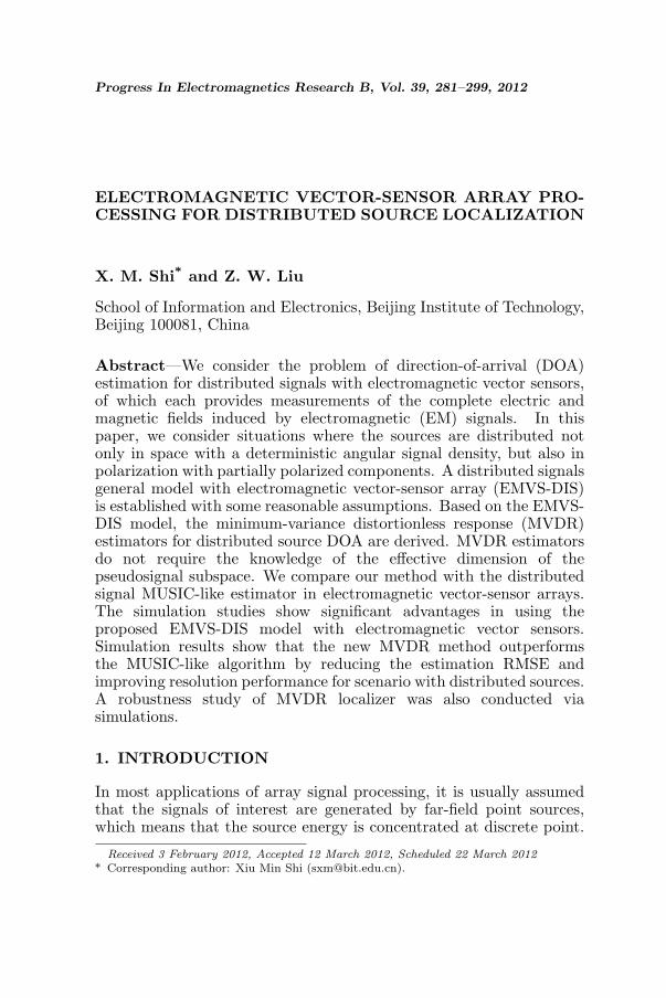
The unit vector rk is pointed from the origin in Cartesian coordinatestoward the source, as depicted in Figure 1. rk can be expressed asfollows:

rk =

[uk

vk

wk

]=

[sin θk cosϕk

sin θk sinϕk

cos θk

](1)

where 0 ≤ θk < π denotes the signal’s elevation angle; 0 ≤ ϕk < 2πsymbolizes the azimuth angle.

2.1. Point Sources Model

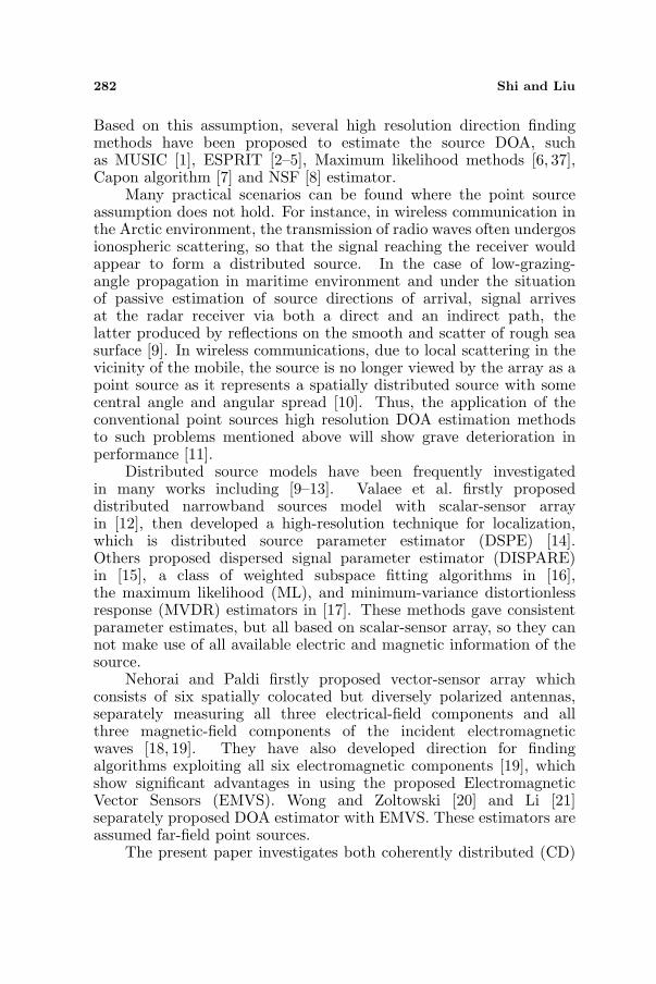
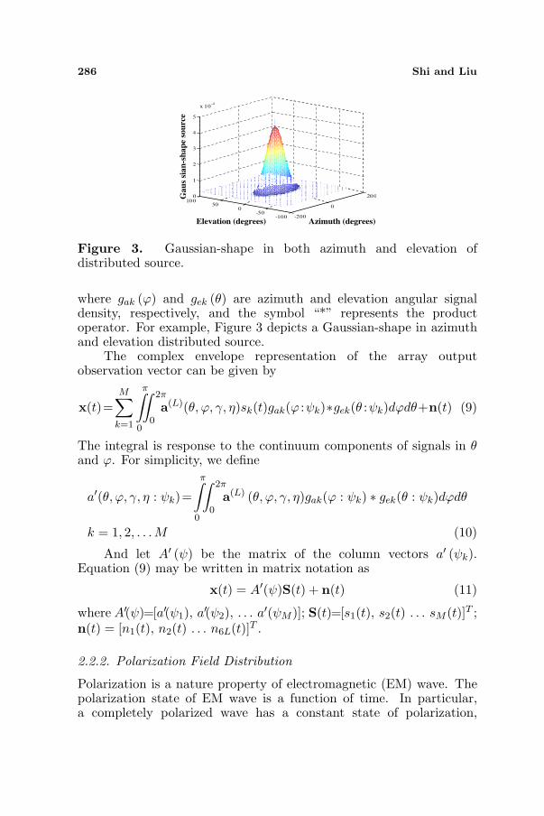
Uncorrelated transverse electromagnetic plane waves impinge upona three-dimensional (3-D) array of identically oriented L elementselectromagnetic vector-sensors. The L elements along the y-axis withd (half wave length) inter-element spacing were chosen (see Figure 2).Every sensor consists of six spatially colocated but diversely polarizedantennas, namely, three electric and three magnetic orthogonal sensors(dipoles and loops).

The complex envelope of the array output has three electric-fieldvectors, and three magnetic-field vectors may expressed in Cartesian

284 Shi and Liu

x

y

z

O

k

k

-rkθ

ϕ

Figure 1. The unit vector rk.

ϕ

θ

d

z

z

x

x

y

y

Figure 2. Electromagnetic vec-tor sensors array.

coordinates as

x(t)=[x1(t), x2(t) . . . x6L(t)]T =M∑

k=1

a(L) (θk, ϕk, γk, ηk)sk(t) + n(t) (2)

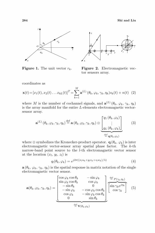
where M is the number of cochannel signals, and a(L) (θk, ϕk, γk, ηk)is the array manifold for the entire L-elements electromagnetic vector-sensor array.

a(L) (θk, ϕk, γk, ηk)def= a (θk, ϕk, γk, ηk)⊗

q1 (θk, ϕk)...

qL (θk, ϕk)

︸︷︷︸def= q(θk,ϕk)

(3)

where ⊗ symbolizes the Kronecker-product operator. q (θk, ϕk) is interelectromagnetic vector-sensor array spatial phase factor. The k-thnarrow-band point source to the l-th electromagnetic vector sensorat the location (xl, yl, zl) is

ql(θk, ϕk) = ej2π((xluk+ylvk+zlwk)/λ) (4)

a (θk, ϕk, γk, ηk) is the spatial response in matrix notation of the singleelectromagnetic vector sensor.

a(θk, ϕk, γk, ηk) =

cosϕk cos θk − sinϕk

sinϕk cos θk cosϕk

− sin θk 0− sinϕk − cosϕk cos θk

cosϕk − sinϕk cos θk

0 sin θk

︸︷︷︸def= V(θk,ϕk)

def= P (γk,ηk)︷︸︸︷[sin γke

jηk

cos γk

](5)


where 0 ≤ γk < π/2 represents the auxiliary polarization angle;0 ≤ ηk < 2π signifies the polarization phase difference.

Note that V (θk, ϕk) depend only on the sources’ spatial angularlocations, and P (γk, ηk) depend only on the incident signals’polarization states.

Equation (2) may be written in matrix notation as

x(t) = [x1(t), x2(t) . . . x6L(t)]T = AS(t) + n(t) (6)where

A=[a(L)(θ1,ϕ1,γ1,η1), a(L)(θ2,ϕ2,γ2,η2), . . . a(L)(θM ,ϕM ,γM ,ηM )

]

S(t)=[s1(t), s2(t) . . . sM (t)]T n(t) = [n1(t), n2(t) . . . n6L(t)]T

n (t) symbolizes the 6L × 1 additive complex-valued zero-meanwhite noise vector.

2.2. Models for Distributed Sources

Consider a three-dimensional array of L elements EMVS (see Figure 2)monitoring a wave of M distributed narrowband sources in additivebackground noise. The time dispersion introduced by the multipathand diffusion propagation is assumed to be small in comparison withthe reciprocal of the bandwidth of the emitted signals. Below, wediscuss signal sources, respectively, distribution in spatial field andpolarization field.

2.2.1. Spatial Field Distribution

Firstly we only concern source spatial distribution, under deterministicpolarization state assumption (We will talk about polarization statedistributed property later, and then give completely distributed sourcemodel). The angular signal density of k-th distributed source can bedenoted [14] as

s(θ, ϕ; ψk) = skg(θ, ϕ : ψk) (7)The random component sk represents the temporal behavior of

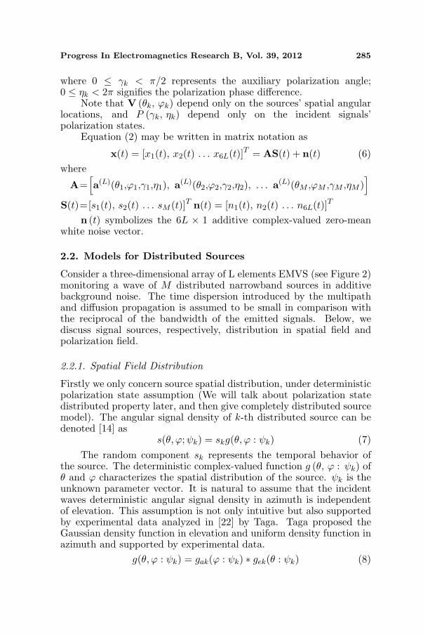
the source. The deterministic complex-valued function g (θ, ϕ : ψk) ofθ and ϕ characterizes the spatial distribution of the source. ψk is theunknown parameter vector. It is natural to assume that the incidentwaves deterministic angular signal density in azimuth is independentof elevation. This assumption is not only intuitive but also supportedby experimental data analyzed in [22] by Taga. Taga proposed theGaussian density function in elevation and uniform density function inazimuth and supported by experimental data.

g(θ, ϕ : ψk) = gak(ϕ : ψk) ∗ gek(θ : ψk) (8)

286 Shi and Liu

-200

0

200

-100-50

050

100

0

1

2

3

4

5

x 10-4

Elevation (degrees) Azimuth (degrees)

Gau

s si

an

-sh

ap

e s

ou

rce

Figure 3. Gaussian-shape in both azimuth and elevation ofdistributed source.

where gak (ϕ) and gek (θ) are azimuth and elevation angular signaldensity, respectively, and the symbol “*” represents the productoperator. For example, Figure 3 depicts a Gaussian-shape in azimuthand elevation distributed source.

The complex envelope representation of the array outputobservation vector can be given by

x(t)=M∑

k=1

π∫

0

∫ 2π

0a(L)(θ, ϕ, γ, η)sk(t)gak(ϕ :ψk)∗gek(θ :ψk)dϕdθ+n(t) (9)

The integral is response to the continuum components of signals in θand ϕ. For simplicity, we define

a′(θ, ϕ, γ, η : ψk)=

π∫

0

∫ 2π

0a(L) (θ, ϕ, γ, η)gak(ϕ : ψk) ∗ gek(θ : ψk)dϕdθ

k = 1, 2, . . .M (10)

And let A′ (ψ) be the matrix of the column vectors a′ (ψk).Equation (9) may be written in matrix notation as

x(t) = A′(ψ)S(t) + n(t) (11)

where A′(ψ)=[a′(ψ1), a′(ψ2), . . . a′(ψM )]; S(t)=[s1(t), s2(t) . . . sM (t)]T ;n(t) = [n1(t), n2(t) . . . n6L(t)]T .

2.2.2. Polarization Field Distribution

Polarization is a nature property of electromagnetic (EM) wave. Thepolarization state of EM wave is a function of time. In particular,a completely polarized wave has a constant state of polarization,


whereas a partially polarized signal varies with time. In a varietyof applications, partially polarized or unpolarized signals are a generaltype of EM wave, and only a limited case of scenario’s signal is acompletely polarized EM wave. For example, as the transmittingRadar rotates itself to scan over the desired sector, the polarizationof signals received at an observation point varies with time [23–28],even though the original transmitted wave is completely polarized.This variation occurs because of the nonstationary behavior oftargets, clutter, rough surface, and other disturbance sources. Inwireless communication in the Arctic environment, the transmissionof signals is often undergone ionospheric scattering, so that thepolarization of signals reaching the receiver would appear to bepartially polarized [29, 30]. In maritime environments, tracking targetsflying near the sea surface is a case of low-grazing-angle propagation.The polarization of signals received is partially polarized while the seasurface is disturbed and irregular [9].

Under the unknown polarization stochastic state, we decomposescattering partially polarized signal into completely polarized andunpolarized two components, to correct the situation mentioned inSection 2.2.1 that does not concern source polarization distributiondeficiency. The completely polarized component relates to the directsignal, and the unpolarized component is associated with the diffusesignal component. We conduct decomposition to signal and express itas [38]

ps = pcpppH + pup/2∗I2 (12)

where pcp = σ2S = E[|sk(t)|2]; pup = σ2

u = E[|UHk (t) ∗ Uk(t)|];

Uk(t) ∈ C2X1.p is the polarization vector defined as in (5); Uk(t) denotes the

horizontal and vertical components of the diffuse signal, and they areuncorrelated. The diffuse component carries no useful message, butit provides information about the source spatial position. Hence, thiscomponent accounts for “signal” in the model, instead of as part of thenoise. Then, the array output can be written as

x(t) =M∑

k=1

π∫

0

∫ 2π

0a(L) (θ, ϕ, γ, η)gak(ϕ : ψk) ∗ gek(θ : ψk)sk(t)dϕdθ

+M∑

k=1

π∫

0

∫ 2π

0V (θ, ϕ)⊗q (θ, ϕ) gak(ϕ :ψk)∗gek(θ :ψk)Uk(t)dϕdθ+n(t)(13)

288 Shi and Liu

For simplicity, we define

b(L)(θk, ϕk) = V (θ, ϕ)⊗ q (θ, ϕ) ;

b′(θ, ϕ : ψk) =

π∫

0

∫ 2π

0V (θ, ϕ)⊗ q (θ, ϕ) gak(ϕ : ψk) ∗ gek(θ : ψk)dϕdθ

k = 1, 2, . . . M (14)

where b′(ψk) ∈ C6LX2. let B (ψ) be the matrix of the column vectorsa′ (ψk) and b′ (ψk).

B(ψ) =[a′(ψ1), a′(ψ2), . . . a′(ψM ),b′(ψ1) . . .b′(ψM )

](15)

Equation (13) may be written in matrix notation as

x(t) = B(ψ)U(t) + n(t) (16)

where U(t) = [s1(t), s2(t) . . . sM (t), UT1 (t), UT

2 (t) . . . UTM (t)]T ; n(t) =

[n1(t), n2(t) . . . n6L(t)]T .We assume that the signal sk (t), noise nk (t) and “signal” UT

k (t)are mutually independent distributed complex Gaussian processes withzero mean. Then, the data model (16) allows us to write the covariancematrix of the array measurements as

R= E(xxH) = Rs (ψ) + Rn (17)

where E(·) denotes statistical expectation; superscript H representsHermitian transposition; the noise covariance matrix is Rn = σ2

nI; σ2n

is the noise power; Rs (ψ) is the noise-free covariance matrix and canbe given by

Rs(ψ) =M∑

k=1

M∑

l=1

π∫

0

2π∫

0

π∫

0

∫ 2π

0a(L)(ψk)skpkl

(θ,ϕ,θ′,ϕ′ :ψk,ψl

)s∗l a

(L)(ψl)Hdϕdθdϕ′dθ′+

M∑

k=1

M∑

l=1

π∫

0

2π∫

0

π∫

0

∫ 2π

0b(L)(ψk)Ukpkl

(θ,ϕ,θ′,ϕ′:ψk,ψl

)U∗

l b(L)(ψl)Hdϕdθdϕ′dθ′ (18)

where

pkl

(θ,ϕ,θ′,ϕ′:ψk,ψl

)=gak(ϕ :ψk)∗ gek(θ :ψk)∗ g∗al(ϕ

′ :ψl)∗ g∗el(θ′:ψl) (19)

and “*” represents the complex conjugation. If the signals fromdifferent sources are uncorrelated, then

pkl

(θ, ϕ, θ′, ϕ′ : ψk, ψl

)= pk

(θ, ϕ, θ′, ϕ′ : ψk

)δkl

= gak(ϕ : ψk) ∗ gek(θ : ψk) ∗ g∗ak

(ϕ′ : ψk

) ∗ g∗ek(θ′ : ψk

)(20)


The noise-free covariance matrix is then given by

Rs(ψ)

=M∑

k=1

π∫

0

2π∫

0

π∫

0

∫ 2π

0a(L) (ψk) skpk

(θ,ϕ,θ′,ϕ′ :ψk

)s∗ka

(L) (ψk)Hdϕdθdϕ′dθ′

+M∑

k=1

π∫

0

2π∫

0

π∫

0

∫ 2π

0b(L)(ψk)Ukpk

(θ,ϕ,θ′,ϕ′:ψk

)U∗

kb(L)(ψk)Hdϕdθdϕ′dθ′ (21)

Below, we discuss Equation (21) in CD and ID sources, respectively.For CD sources, the noise-free covariance matrix can be given by

Rs(ψ) =M∑

k=1

a′(θ, ϕ, γ, η : ψk)σsa′ (θ′, ϕ′, γ, η : ψk

)H

+M∑

k=1

b′ (θ, ϕ : ψk) σub′(θ′, ϕ′ :ψk

)H (22)

For ID sources,

pk

(θ, ϕ, θ′, ϕ′ : ψk

)=pk (θ, ϕ, : ψk) δ

(θ − θ′

)δ(ϕ− ϕ′

)

=gak(ϕ :ψk)∗ gek(θ :ψk)∗g∗ak(ϕ :ψk)∗ g∗eK(θ :ψk)(23)

Then the noise-free covariance matrix can be given by

Rs (ψ) = σ2s

M∑

k=1

π∫

0

∫ 2π

0a(L) (ψk)pk (θ, ϕ : ψk)a(L)(ψk)Hdϕdθ

+σ2u

M∑

k=1

π∫

0

∫ 2π

0b(L) (ψk)pk (θ, ϕ : ψk)b(L) (ψk)

Hdϕdθ (24)

3. MVDR LOCALIZER

By performing an eigen decomposition of correlation matrix in (17),we get

R = UsΣsUHs + UnΣnUH

n (25)

where Σs = diag(σ2

S1, σ2S2 . . . σ2

SM , σ2u1

/2, σ

2u1

/2 . . . σ

2uM

/2, σ

2uM

/2).

Σs denotes a 3M×3M diagonal matrix whose diagonal entries arethe 3M largest eigenvalues, and Σn symbolizes a (6L−3M)×(6L−3M)diagonal matrix whose diagonal entries contains the (6L−3M) smallest

290 Shi and Liu

eigenvalues σ2n. Signal subspace Us is 3M eigenvectors (6L×1), and Un

denotes 6L× (6L−3M) matrix composed of the remaining (6L−3M)eigenvectors of correlation matrix and is the pseudo-noise subspace.[ϕk, θk, γk, ηk, σ2

S , σ2u, σ2

n] are unknown parameters, and the vectorψ = [ϕk, θk, γk, ηk] includes parameters of interest.

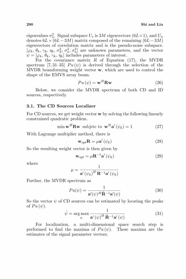
For the covariance matrix R of Equation (17), the MVDRspectrum [7, 31–35] Pu (ψ) is derived through the selection of theMVDR beamforming weight vector w, which are used to control theshape of the EMVS array beam.

Pu (ψ) = wHRw (26)

Below, we consider the MVDR spectrum of both CD and IDsources, respectively.

3.1. The CD Sources Localizer

For CD sources, we get weight vector w by solving the following linearlyconstrained quadratic problem.

minwHRw subjetc to wHa′ (ψk) = 1 (27)

With Lagrange multiplier method, there is

woptR = µa′ (ψk) (28)

So the resulting weight vector is then given by

wopt = µR−1a′ (ψk) (29)

whereµ =

1

a′ (ψk)H R−1a′ (ψk)

Further, the MVDR spectrum as

Pu(ψ) =1

a′(ψ)HR̂−1a′(ψ)(30)

So the vector ψ of CD sources can be estimated by locating the peaksof Pu (ψ).

ψ̂ = arg maxψ

1

a′ (ψ)H R̂−1a′ (ψ)(31)

For localization, a multi-dimensional space search step isperformed to find the maxima of Pu (ψ). These maxima are theestimates of the signal parameter vectors.


3.2. The ID Sources Localizer

For simplicity, from Equation (24) we define

pak(ψk) =

π∫

0

∫ 2π

0a(L) (ψk)pk (θ, ϕ : ψk)a(L) (ψk)

H dϕdθ (32)

pbk(ψk) =

π∫

0

∫ 2π

0b(L) (ψk)pk (θ, ϕ : ψk)b(L) (ψk)

H dϕdθ (33)

We assume that the sources’ powers are equal. Equation (24) simplifiesto

Rs (ψ) = σs

M∑

k=1

pak (ψk) + σu

M∑

k=1

pbk (ψk) (34)

For ID sources, we extend the MVDR Capon spatial filter[31] to theEMVS-DIS model as

minwHRw subjetc to wHp (ψk)w = 1 (35)

where p (ψk) = pak (ψk) + εpbk (ψk), ε is a ratio of diffuse componentsto direct components in induced signals. Equation (35) maintainsdistortionless spatial response to a hypothetical source’s covariancematrix with the unknown vector parameter of interest, while maximallysuppressing the contribution of interference sources and noise.

With Lagrange multiplier method, there is

Rw = µp (ψk)w (36)

Multiplying Equation (36) by wH from left and using the constraintof (35), we obtain that

µ = wHRw = Pu(ψ) (37)

Therefore, the smallest generalized eigenvalue of the matrix pencil{R, P(ψk)} is equal to the minimal value of the objective functionPu (ψ).

Then the MVDR spectrum as

Pu (ψ) = λmin({R,P (ψk)}) (38)

So the vector ψ of ID sources can be estimated by locating the peaksof

ψ̂ = arg maxψ

1λmax({R−1P (ψk)}) (39)

The parameter vector estimates can be obtained from the maximaof (39). Generally, a multi-dimensional search is required.

292 Shi and Liu

4. SIMULATION RESULTS

In this section, we evaluate the performance of the proposed techniquesin different scenarios. We consider an EMVS array that comprisesseveral colocated vector sensors as Figure 2, measuring all threeelectrical-field components and all three magnetic-field components.Each sensor is aligned with the axis y of the Cartesian coordinatesystem with element spacing d = λ/2 (λ is the wavelength at theoperating frequency). The azimuth angular signal density of sources isassumed to be uniform.

gak(ϕ) =

12∆1k

, |ϕ− ϕk| < ∆1k

0, otherwise(40)

∆1k is the extension width of uniform density, and ϕk is centralangle of arrival. The elevation angular signal density of the sources isassumed to be Gaussian density

gek(θ) =1√

2π∆2k

exp(−(θ − θk)2

2∆22k

)(41)

where θk and ∆2k are the central angle of arrival and the extensionwidth of Gaussian density, respectively.

In our simulation, the additive white noise is, zero mean, complexGaussian. SNR is defined as

SNR = (1/M)M∑

k=1

([|sk(t)|2

]+

∣∣UHk (t) ∗ Uk(t)

∣∣)

/σ2n (42)

In the first scenario, two equal power CD sources impinge upon a2-element EMVS array, with the following parameters values:

ϕ1 = 25◦ ϕ2 = 26◦; θ1= 20◦ θ2= 45◦;∆11 = 0.5◦ ∆21 = 1.0◦; ∆12 = 0.5◦ ∆22 = 1.0◦.

The polarization states are

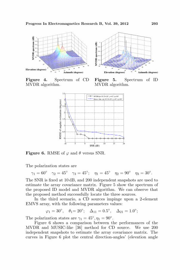
γ1 = 60◦ γ2 = 45◦; η1 = 45◦ η2 = 90◦.The SNR is fixed at 10 dB, and 200 independent snapshots are

used to estimate the array covariance matrix. Figure 4 shows thespectrum of the proposed CD model and MVDR algorithm. We canobserve that the proposed method successfully locates the two sources.

In the second scenario, three equal power ID sources impinge upona 2-element EMVS array, with the following parameters values:

ϕ1 = 45◦ ϕ2 = 60◦ ϕ3 = 30◦; θ1= 35◦ θ2= 45◦ θ3= 20◦;∆11 = ∆12 = ∆13 = 0.5◦; ∆21 = ∆22 = ∆23 = 1.0◦.


-100

1020

3040

5060

-20

0

20

40

60

0

0.2

0.4

0.6

0.8

1

Elevation (degrees)

Azimuth (degrees)

MV

DR

sp

ectr

um

(d

B)

Figure 4. Spectrum of CDMVDR algorithm.

20

30

40

50

60

70

1020

3040

5060

0

0.2

0.4

0.6

0.8

1

Elevation (degrees) Azimuth (degrees)

MV

DR

sp

ectr

um

(d

B)

Figure 5. Spectrum of IDMVDR algorithm.

-10 -5 0 5 10 15 20

0

0.5

1

1.5

2

2.5

3

3.5

SNR (dB)

RM

SE

of

angu

lar

esti

mati

on

(deg

rees

)

MVDR-φ=30°,θ=20°,γ=45°,η=90°

Music-like--φ=30°,θ=20°,γ=45°,η=90°

Figure 6. RMSE of ϕ and θ versus SNR.

The polarization states are

γ1 = 60◦ γ2 = 45◦ γ3 = 45◦; η1 = 45◦ η2 = 90◦ η3 = 30◦.

The SNR is fixed at 10 dB, and 200 independent snapshots are used toestimate the array covariance matrix. Figure 5 show the spectrum ofthe proposed ID model and MVDR algorithm. We can observe thatthe proposed method successfully locate the three sources.

In the third scenario, a CD sources impinge upon a 2-elementEMVS array, with the following parameters values:

ϕ1 = 30◦, θ1= 20◦; ∆11 = 0.5◦, ∆21 = 1.0◦;

The polarization states are γ1 = 45◦, η1 = 90◦.Figure 6 shows a comparison between the performances of the

MVDR and MUSIC-like [36] method for CD source. We use 200independent snapshots to estimate the array covariance matrix. Thecurves in Figure 6 plot the central direction-angles’ (elevation angle

294 Shi and Liu

and azimuth angle) composite estimation Root Mean-Square Error(RMSE) at various signal-to-noise ratio (SNR) levels, using the MVDRand MUSIC-like method. The RMSE is computed by taking squareroot of the mean of the respective variances of ϕ and θ, and theRMSE of all the following figures in this paper is similarly computed.The performances of all estimations are obtained by means of 100independent Monte Carlo simulation experiments.

From Figure 6 one can observe that the MVDR localizer is superiorto the MUSIC-like method at all SNRs, and for SNR above 2 dBestimation RMSE decreased nearly to zero.

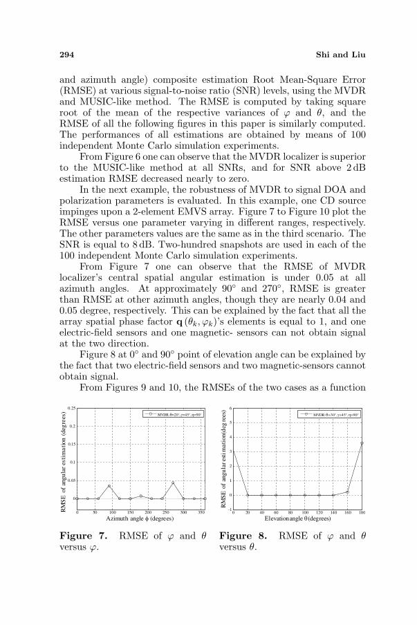
In the next example, the robustness of MVDR to signal DOA andpolarization parameters is evaluated. In this example, one CD sourceimpinges upon a 2-element EMVS array. Figure 7 to Figure 10 plot theRMSE versus one parameter varying in different ranges, respectively.The other parameters values are the same as in the third scenario. TheSNR is equal to 8 dB. Two-hundred snapshots are used in each of the100 independent Monte Carlo simulation experiments.

From Figure 7 one can observe that the RMSE of MVDRlocalizer’s central spatial angular estimation is under 0.05 at allazimuth angles. At approximately 90◦ and 270◦, RMSE is greaterthan RMSE at other azimuth angles, though they are nearly 0.04 and0.05 degree, respectively. This can be explained by the fact that all thearray spatial phase factor q (θk, ϕk)’s elements is equal to 1, and oneelectric-field sensors and one magnetic- sensors can not obtain signalat the two direction.

Figure 8 at 0◦ and 90◦ point of elevation angle can be explained bythe fact that two electric-field sensors and two magnetic-sensors cannotobtain signal.

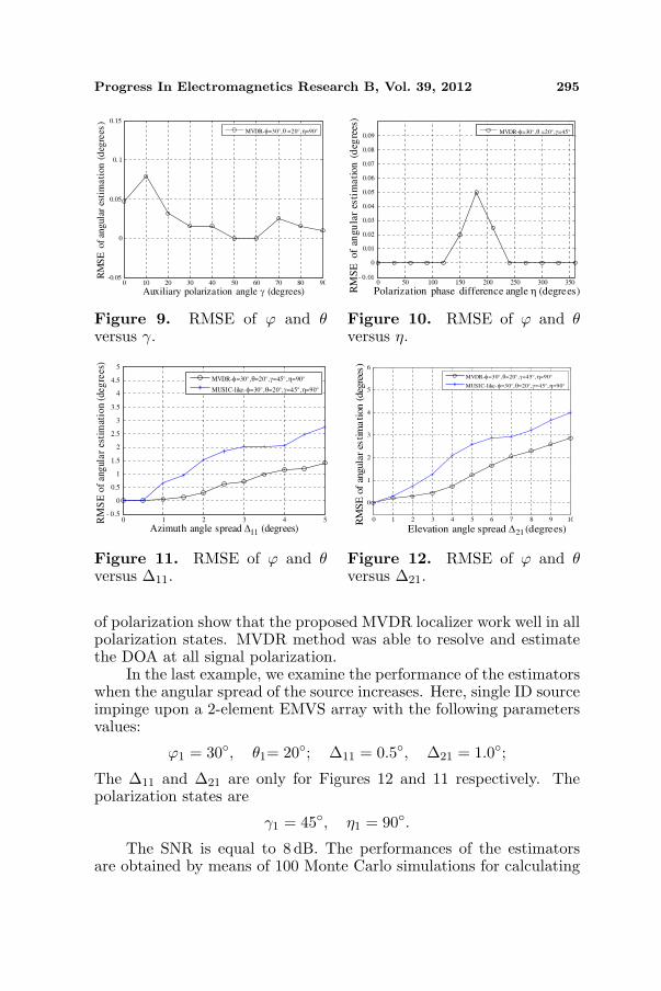
From Figures 9 and 10, the RMSEs of the two cases as a function

0 50 100 150 200 250 300 350

0

0.05

0.1

0.15

0.2

0.25

Azimuth angle φ (degrees)

RM

SE

of

angu

lar

esti

ma

tion

(deg

rees

)

MVDR-θ=20°,γ=45°,η=90°

Figure 7. RMSE of ϕ and θversus ϕ.

0 20 40 60 80 100 120 140 160 180-1

0

1

2

3

4

5

6

Elevation angle θ (degrees)

RM

SE

of

angu

lar es

tim

ati

on (d

egre

es)

MVDR-θ=30°,γ=45°,η=90°

Figure 8. RMSE of ϕ and θversus θ.


0 10 20 30 40 50 60 70 80 90-0.05

0

0.05

0. 1

0.15

Auxiliary polarization angle γ (degrees)

RM

SE

of

angula

r es

tim

ati

on

(d

egre

es)

MVDR-φ=30°,θ =20°,η=90°

Figure 9. RMSE of ϕ and θversus γ.

0 50 100 150 200 250 300 350- 0.01

0

0.01

0.02

0.03

0.04

0.05

0.06

0.07

0.08

0.09

Polarization phase difference angle η (degrees)RM

SE

of

angu

lar

esti

mati

on

(d

egre

es)

MVDR-φ=30°,θ =20°,γ=45°

Figure 10. RMSE of ϕ and θversus η.

0 1 2 3 4 5- 0.5

0

0.5

1

1.5

2

2.5

3

3.5

4

4.5

5

Azimuth angle spread ∆11 (degrees)

RM

SE

of

ang

ular

esti

mat

ion

(deg

rees

)

MVDR-φ=30°,θ=20°,γ=45°,η=90°

MUSIC-like-φ=30°,θ=20°,γ=45°,η=90°

Figure 11. RMSE of ϕ and θversus ∆11.

0 1 2 3 4 5 6 7 8 9 10

0

1

2

3

4

5

6

Elevation angle spread ∆21 (degrees)

RM

SE

of

angula

r es

tim

ati

on (

deg

rees

)

MVDR-φ=30°,θ=20°,γ=45°,η=90°

MUSIC-like-φ=30°,θ=20°,γ=45°,η=90°

Figure 12. RMSE of ϕ and θversus ∆21.

of polarization show that the proposed MVDR localizer work well in allpolarization states. MVDR method was able to resolve and estimatethe DOA at all signal polarization.

In the last example, we examine the performance of the estimatorswhen the angular spread of the source increases. Here, single ID sourceimpinge upon a 2-element EMVS array with the following parametersvalues:

ϕ1 = 30◦, θ1= 20◦; ∆11 = 0.5◦, ∆21 = 1.0◦;

The ∆11 and ∆21 are only for Figures 12 and 11 respectively. Thepolarization states are

γ1 = 45◦, η1 = 90◦.

The SNR is equal to 8 dB. The performances of the estimatorsare obtained by means of 100 Monte Carlo simulations for calculating

296 Shi and Liu

the RMSE. The number of snapshots used to estimate the samplecovariance matrix is 200.

Figures 11 and 12 show the RMS error of central spatial angularestimates versus the angular spread of azimuth and elevation angle.The two figures show a comparison between the performance ofthe MVDR and MUSIC-like method. We can observe that theproposed MVDR localizer is robust in the single-source case andwidely separated sources situation. The proposed estimator hasgreat advantage relative to MUSIC-like method, which do require theknowledge of the effective dimension of the pseudosignal subspace.

5. CONCLUSIONS

A new EMVS-DIS Model for the distributed signals source hasbeen presented. In this model, we proposed decomposing thedistributed signals into polarized and unpolarized components for itspolarization state “distribution” and describing spatial distributionwith deterministic angular signal density. We have presented thatit is possible to significantly reduce the RMSE of the central DOAparameters estimation with EMVS-DIS Model when the full EMinformation is exploited using electromagnetic vector sensors. Theproposed MVDR algorithm does not require the knowledge of effectivedimension of the pseudosignal subspace, which is the main difficultyof the existing subspace estimators. This character is extremelyimportant to ID source parameter estimation. Furthermore, we showedthat the performance of the proposed MVDR parametric estimationalgorithm is super than MUSIC-like method by simulations. Theproposed estimator exploits independent polarization information aswell as azimuth and elevation angle (spatial information) of the source,and it exhibits a better estimation performance.

REFERENCES

1. Schmidt, R. O., “Multiple emitter location and signal parameterestimation,” Proceedings of International Conference of RADCSpectral Estim. Workshop, 234–258, 1979.

2. Schmidt, R. O., “Multiple emitter location and signal parameterestimation,” IEEE Trans. on Antennas and Propag., Vol. 34,No. 3, 276–280, 1986.

3. Roy, R. and T. Kailath, “ESPRIT — Estimation of signalparameters via rotational invariance techniques,” IEEE Trans.Acoust. Speech, Signal Processing, Vol. 37, No. 7, 984–995,Jul. 1989.


4. Yang, P., F. Yang, and Z.-P. Nie, “DOA estimation with sub-array divided technique and interporlated esprit algorithm on acylindrical conformal array antenna,” Progress In Electromagnet-ics Research, Vol. 103, 201–216, 2010.

5. Bencheikh, M. L. and Y. Wang, “Combined esprit-root musicfor DOA-DOD estimation in polarimetric bistatic MIMO radar,”Progress In Electromagnetics Research Letters, Vol. 22, 109–117,2011.

6. Stoica, P. and K. C. Sharman, “Maximum likelihood methods fordirection-of-arrival estimation,” IEEE Trans. on Acoust. Speech,Signal Processing, Vol. 38, No. 7, 1132–1142, Jul. 1990.

7. Capon, J. “High-resolution frequency-wave number spectrumanalysis,” Proceedings of the IEEE, Vol. 57, 1408–1418, 1969.

8. Viberg, M. and B. Ottersten, “Sensor array processing based onsubspace fitting,” IEEE Trans. on Signal Processing, Vol. 39,No. 5, 1110–1121, May 1991.

9. Hurtado, M. and A. Nehorai, “Performance analysis of passivelow-grazing-angle source localization in maritime environmentsusing vector sensors,” IEEE Trans. on Aerospace and ElectronicSystems, Vol. 43, No. 4, 780–789, Apr. 2007.

10. Kalliola, K., K. Sulonen, and H. Laitinen, “Angular powerdistribution and mean effective gain of mobile antenna indifferent propagation environments,” IEEE Trans. on VehicularTechnology, Vol. 51, No. 5, 823–837, 2002.

11. Astely, D. and B. Ottersten, “The effects of local scattering ondirection of arrival estimation with MUSIC,” IEEE Trans. onSignal Processing, Vol. 47, No. 12, 3220–3234, Dec. 1999.

12. Valaee, S., P. Kabal, and B. Champagne, “Localization ofdistributed sources,” Proceedings of 14th GRETSI Symp. SignalImage Processing, 289–292, Julan-les-Pins, France, Sep. 1993.

13. Park, G. M., H. G. Lee, and S. Y. Hong, “Doa resolutionenhancement of coherent signals via spatial averaging ofvirtually expanded arrays,” Journal of Electromagnetic Waves andApplications, Vol. 24, No. 1, 61–70, 2010.

14. Valaee, S., B. Champagne, and P. Kabal, “Parametric localizationof distributed sources,” IEEE Trans. on Signal Processing, Vol. 43,No. 9, 2144–2153, 1995.

15. Meng, Y., P. Stoica, and K. M.Wong, “Estimation of thedirections of arrival of spatially dispersed signals in arrayprocessing,” IEE Proc. of Radar, Sonar and Navigation, Vol. 143,No. 1, 1–9, Feb. 1996.

298 Shi and Liu

16. Bengtsson, M., “Antenna array processing for high rank datamodels,” Ph.D. dissertation, Royal Institute of Technology,Stockholm, Sweden, 1999.

17. Rahamim, D. and J. Tabrikian, “Source localization using vectorsensor array in a multipath environment,” IEEE Trans. on SignalProcessing, Vol. 52, No. 11, 3096–3103, 2004.

18. Nehorai, A. and E. Paldi, “Superresolution compact arrayradiolocation technology (SuperCART) project,” Proceedings ofAsilomar Conference, 566–572, 1991.

19. Nehorai, A. and E. Paldi, “Vector-sensor array processing forelectromagnetic source localization,” IEEE Trans. on SignalProcessing, Vol. 42, No. 2, 376–398, 1994.

20. Wong, K. T. and M. D. Zoltowski, “Closed-form direction findingand polarization estimation with arbitrary spaced electromagneticvector-sensors at unknown location,” IEEE Trans. on Antennasand Propag., Vol. 48, No. 5, 671–681, May 2000.

21. Li, J., “Direction and polarization estimation using arrays withsmall loops and short dipoles,” IEEE Trans. on Antennas andPropag., Vol. 41, No. 3, 379–387, Mar. 1993.

22. Taga, T., “Analysis for mean effective gain of mobile antennasin land mobile radio environments,” IEEE Trans. on VehicularTechnology, Vol. 39, No. 5, 117–131, May 1990.

23. Skolnik, M., Radar Handbook, 2nd edition, McGraw-Hill, 1970.24. Giuli, D., “Polarization diversity in radars,” Proceedings of the

IEEE, Vol. 74, No. 2, 245–269, Feb. 1986.25. Li, J. and P. Stoica, “Efficient parameter estimation of

partially polarized electromagnetic waves,” IEEE Trans. on SignalProcessing, Vol. 42, No. 11, 3114–3125, Nov. 1994.

26. Li, J. and P. Stoica, “Efficient parameter estimation of partiallypolarized electromagnetic waves,” Proceedings of 1994 Acoustics,Speech, and Signal Processing, 89–92, Florida, USA, Apr. 1994.

27. Ho, K. C., K. C Tan, and B. T. G. Tan, “Estimating directions-of-arrival of completely and incompletely polarized signals withelectromagnetic vector sensors,” Proceedings of ICASSP, Vol. 5,2900–2903, May 1996.

28. Ho, K. C., K. C. Tan, and B. T. G. Tan, “Efficient methodfor estimating directions-of-arrival of partially polarized signalswith electromagnetic vector sensors,” IEEE Trans. on SignalProcessing, Vol. 45, No. 10, 2485–2498, Oct. 1997.

29. Eroglu, A. and J. K. Lee, “Wave propagation and dispersion char-acteristics for a nonreciprocal electrically gyrotropic medium,”


Progress In Electromagnetics Research, Vol. 62, 237–260, 2006.30. Zhao, Z. Y. and G. Chen, “The survey of ionospheric scattering

function,” PIERS Online, Vol. 1, No. 4, 22–26, Hangzhou, China,Aug. 2005.

31. Hassanien, A., S. Shahbazpanahi, and A. B. Gershman, “Ageneralized capon estimator for localization of multiple spreadsources,” IEEE Trans. on Signal Processing, Vol. 52, No. 1, 280–283, 2004.

32. Wang, W., R. Wu, and J. Liang, “A novel diagonalloading method for robust adaptive beamforming,” Progress InElectromagnetics Research C, Vol. 18, 245–255, 2011.

33. Liu, F., J. Wang, C. Y. Sun, and R. Du, “Robust MVDRbeamformer for nulling level control via multi-parametricquadratic programming,” Progress In Electromagnetics ResearchC, Vol. 20, 239–254, 2011.

34. Mallipeddi, R., J. P. Lie, S. G. Razul, P. N. Suganthan, andC. M. S. See, “Robust adaptive beamforming based on covariancematrix reconstruction for look direction mismatch,” Progress InElectromagnetics Research Letters, Vol. 25, 37–46, 2011.

35. Zaharis, Z. D. and T. V. Yioultsis, “A novel adaptive beamformingtechnique applied on linear antenna arrays using adaptive mutatedboolean PSO,” Progress In Electromagnetics Research, Vol. 117,165–179, 2011.

36. Shi, X. M. and Y. Y. Wang, “Parameter estimation of distributedsources with electromagnetic vector sensors,” Proceedings of ICSP,203–206, BeiJing, China, Oct. 2008.

37. Zhou, Q.-C., H. Gao, F. Wang, and J. Shi, “ModifiedDOA estimation methods with unknown source number basedon projection pretransformation,” Progress In ElectromagneticsResearch B, Vol. 38, 387–403, 2012.

38. Hochwald, B. and A. Nehorai, “Polarimetric modeling andparameter estimation with applications to remote sensing,” IEEETrans. on Signal Processing, Vol. 43, 1923–1935, Aug. 1995.

electromagnetic vector-sensor array … · a three-dimensional (3-d) array of identically oriented...

Documents