Electromagnetic Wave PropagationLecture 1: Maxwell’s equations

Daniel Sjoberg

Department of Electrical and Information Technology

August 2015

Outline

1 Maxwell’s equations

2 Vector analysis

3 Boundary conditions

4 Conservation laws

5 Conclusions

2 / 31

Outline

1 Maxwell’s equations

2 Vector analysis

3 Boundary conditions

4 Conservation laws

5 Conclusions

3 / 31

International year of light

A few of the equations back then: Nowadays:

p′ = p+df

dt, q′ = q +

dg

dt, r′ = r +

dh

dtJ tot = J +

∂D

∂t

dγ

dy− dβ

dz= 4πp′

dα

dz− dγ

dx= 4πq′

dβ

dx− dα

dy= 4πr′

∇×H = J tot

e+df

dx+dg

dy+dh

dz= 0 ∇ ·D = ρ

de

dt+dp

dx+dq

dy+dr

dz= 0 ∇ · J tot = 0

Note that the original equations are inconsistent.The sign of e needs to change in one of the equations.

4 / 31

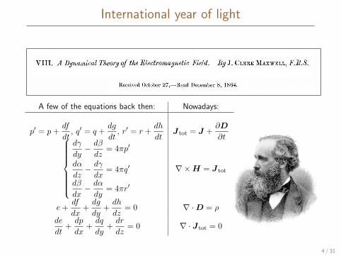
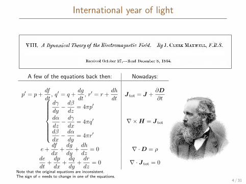
International year of light

A few of the equations back then: Nowadays:

p′ = p+df

dt, q′ = q +

dg

dt, r′ = r +

dh

dtJ tot = J +

∂D

∂t

dγ

dy− dβ

dz= 4πp′

dα

dz− dγ

dx= 4πq′

dβ

dx− dα

dy= 4πr′

∇×H = J tot

e+df

dx+dg

dy+dh

dz= 0 ∇ ·D = ρ

de

dt+dp

dx+dq

dy+dr

dz= 0 ∇ · J tot = 0

Note that the original equations are inconsistent.The sign of e needs to change in one of the equations.

4 / 31

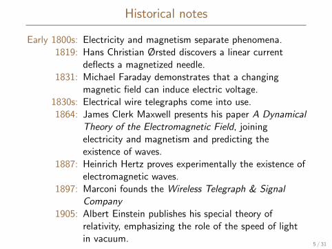
Historical notes

Early 1800s: Electricity and magnetism separate phenomena.1819: Hans Christian Ørsted discovers a linear current

deflects a magnetized needle.1831: Michael Faraday demonstrates that a changing

magnetic field can induce electric voltage.1830s: Electrical wire telegraphs come into use.1864: James Clerk Maxwell presents his paper A Dynamical

Theory of the Electromagnetic Field, joiningelectricity and magnetism and predicting theexistence of waves.

1887: Heinrich Hertz proves experimentally the existence ofelectromagnetic waves.

1897: Marconi founds the Wireless Telegraph & SignalCompany

1905: Albert Einstein publishes his special theory ofrelativity, emphasizing the role of the speed of lightin vacuum.

5 / 31

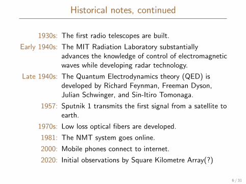
Historical notes, continued

1930s: The first radio telescopes are built.

Early 1940s: The MIT Radiation Laboratory substantiallyadvances the knowledge of control of electromagneticwaves while developing radar technology.

Late 1940s: The Quantum Electrodynamics theory (QED) isdeveloped by Richard Feynman, Freeman Dyson,Julian Schwinger, and Sin-Itiro Tomonaga.

1957: Sputnik 1 transmits the first signal from a satellite toearth.

1970s: Low loss optical fibers are developed.

1981: The NMT system goes online.

2000: Mobile phones connect to internet.

2020: Initial observations by Square Kilometre Array(?)

6 / 31

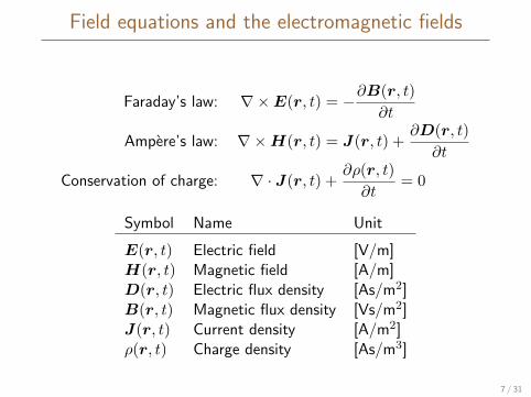
Field equations and the electromagnetic fields

Faraday’s law: ∇×E(r, t) = −∂B(r, t)

∂t

Ampere’s law: ∇×H(r, t) = J(r, t) +∂D(r, t)

∂t

Conservation of charge: ∇ · J(r, t) + ∂ρ(r, t)

∂t= 0

Symbol Name Unit

E(r, t) Electric field [V/m]H(r, t) Magnetic field [A/m]D(r, t) Electric flux density [As/m2]B(r, t) Magnetic flux density [Vs/m2]J(r, t) Current density [A/m2]ρ(r, t) Charge density [As/m3]

7 / 31

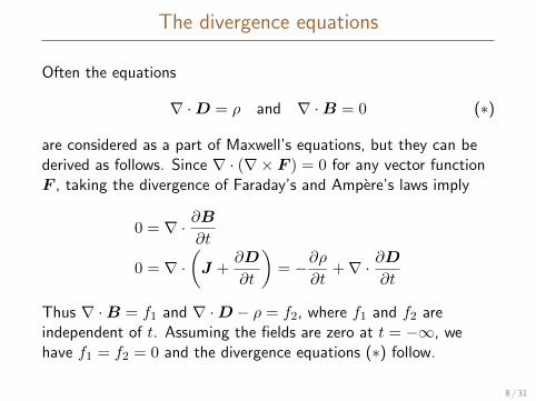
The divergence equations

Often the equations

∇ ·D = ρ and ∇ ·B = 0 (∗)

are considered as a part of Maxwell’s equations, but they can bederived as follows. Since ∇ · (∇× F ) = 0 for any vector functionF , taking the divergence of Faraday’s and Ampere’s laws imply

0 = ∇ · ∂B∂t

0 = ∇ ·(J +

∂D

∂t

)= −∂ρ

∂t+∇ · ∂D

∂t

Thus ∇ ·B = f1 and ∇ ·D − ρ = f2, where f1 and f2 areindependent of t. Assuming the fields are zero at t = −∞, wehave f1 = f2 = 0 and the divergence equations (∗) follow.

8 / 31

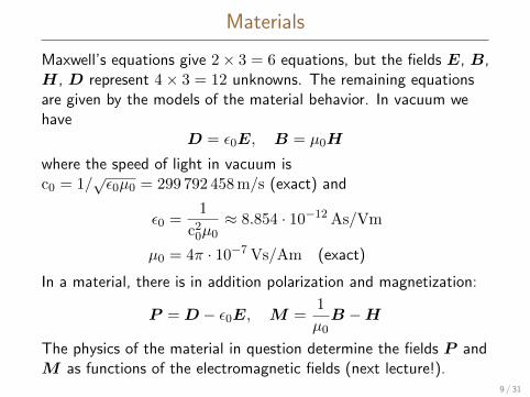
Materials

Maxwell’s equations give 2× 3 = 6 equations, but the fields E, B,H, D represent 4× 3 = 12 unknowns. The remaining equationsare given by the models of the material behavior. In vacuum wehave

D = ε0E, B = µ0H

where the speed of light in vacuum isc0 = 1/

√ε0µ0 = 299 792 458m/s (exact) and

ε0 =1

c20µ0≈ 8.854 · 10−12As/Vm

µ0 = 4π · 10−7Vs/Am (exact)

In a material, there is in addition polarization and magnetization:

P = D − ε0E, M =1

µ0B −H

The physics of the material in question determine the fields P andM as functions of the electromagnetic fields (next lecture!).

9 / 31

Outline

1 Maxwell’s equations

2 Vector analysis

3 Boundary conditions

4 Conservation laws

5 Conclusions

10 / 31

Literature

Here, we give a brief overview of vector analysis used in the course.

A summary of vector relations can be found in Orfanidis,Appendices C–E. If you want more in-depth, you can consult atypical first text book on electromagnetism, like Griffiths or Cheng.

11 / 31

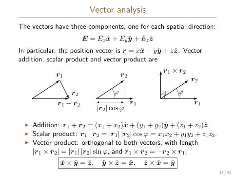
Vector analysis

The vectors have three components, one for each spatial direction:

E = Exx+ Eyy + Ezz

In particular, the position vector is r = xx+ yy + zz. Vectoraddition, scalar product and vector product are

r1 + r2

r1

r2r1

r2

ϕ

|r2| cosϕr1

r2

ϕ

r1 × r2

I Addition: r1 + r2 = (x1 + x2)x+ (y1 + y2)y + (z1 + z2)zI Scalar product: r1 · r2 = |r1| |r2| cosϕ = x1x2 + y1y2 + z1z2.I Vector product: orthogonal to both vectors, with length|r1 × r2| = |r1| |r2| sinϕ, and r1 × r2 = −r2 × r1.

x× y = z, y × z = x, z × x = y

12 / 31

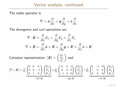
Vector analysis, continued

The nabla operator is

∇ = x∂

∂x+ y

∂

∂y+ z

∂

∂z

The divergence and curl operations are

∇ ·E =∂

∂xEx +

∂

∂yEy +

∂

∂zEz

∇×E =∂

∂xx×E +

∂

∂yy ×E +

∂

∂zz ×E

Cartesian representation: [E] =

(ExEy

Ez

)and

[∇×E] = ∂∂x

0 0 00 0 −10 1 0

Ex

Ey

Ez

︸ ︷︷ ︸

=[x×E]

+ ∂∂y

0 0 10 0 0−1 0 0

Ex

Ey

Ez

︸ ︷︷ ︸

=[y×E]

+ ∂∂z

0 −1 01 0 00 0 0

Ex

Ey

Ez

︸ ︷︷ ︸

=[z×E]

13 / 31

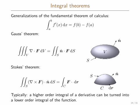
Integral theorems

Generalizations of the fundamental theorem of calculus:∫ b

af ′(x) dx = f(b)− f(a)

Gauss’ theorem:

∫∫∫V∇ · F dV =

∫∫Sn · F dS

n

V

S

Stokes’ theorem:

∫∫S(∇× F ) · ndS =

∫CF · dr

nS

C dr

Typically: a higher order integral of a derivative can be turned intoa lower order integral of the function.

14 / 31

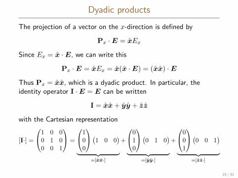
Dyadic products

The projection of a vector on the x-direction is defined by

Px ·E = xEx

Since Ex = x ·E, we can write this

Px ·E = xEx = x(x ·E) = (xx) ·E

Thus Px = xx, which is a dyadic product. In particular, theidentity operator I ·E = E can be written

I = xx+ yy + zz

with the Cartesian representation

[I·] =

1 0 00 1 00 0 1

=

100

(1 0 0)

︸ ︷︷ ︸=[xx·]

+

010

(0 1 0)

︸ ︷︷ ︸=[yy·]

+

001

(0 0 1)

︸ ︷︷ ︸=[zz·]

15 / 31

Outline

1 Maxwell’s equations

2 Vector analysis

3 Boundary conditions

4 Conservation laws

5 Conclusions

16 / 31

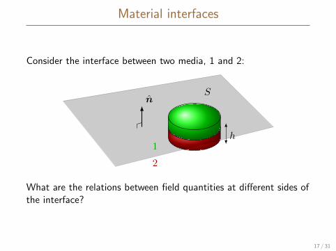
Material interfaces

Consider the interface between two media, 1 and 2:

n

h

S

1

2

What are the relations between field quantities at different sides ofthe interface?

17 / 31

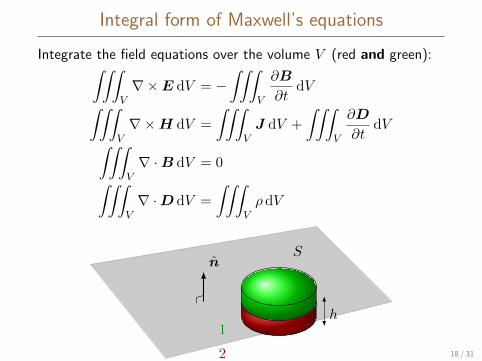
Integral form of Maxwell’s equations

Integrate the field equations over the volume V (red and green):∫∫∫V∇×E dV = −

∫∫∫V

∂B

∂tdV∫∫∫

V∇×H dV =

∫∫∫VJ dV +

∫∫∫V

∂D

∂tdV∫∫∫

V∇ ·B dV = 0∫∫∫

V∇ ·D dV =

∫∫∫VρdV

n

h

S

1

2 18 / 31

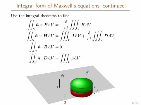
Integral form of Maxwell’s equations, continued

Use the integral theorems to find∫∫Sn×E dV = − d

dt

∫∫∫VB dV∫∫

Sn×H dV =

∫∫∫VJ dV +

d

dt

∫∫∫VD dV∫∫

Sn ·B dV = 0∫∫

Sn ·D dV =

∫∫∫VρdV

n

h

S

1

2 19 / 31

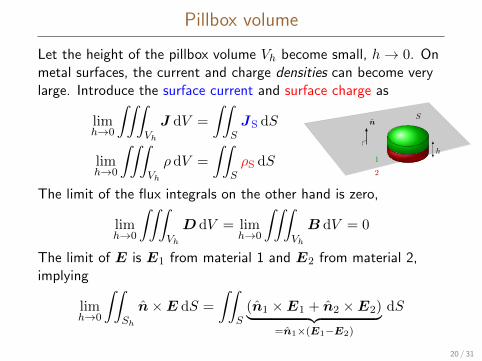
Pillbox volume

Let the height of the pillbox volume Vh become small, h→ 0. Onmetal surfaces, the current and charge densities can become verylarge. Introduce the surface current and surface charge as

n

h

S

1

2

limh→0

∫∫∫Vh

J dV =

∫∫SJS dS

limh→0

∫∫∫Vh

ρ dV =

∫∫SρS dS

The limit of the flux integrals on the other hand is zero,

limh→0

∫∫∫Vh

D dV = limh→0

∫∫∫Vh

B dV = 0

The limit of E is E1 from material 1 and E2 from material 2,implying

limh→0

∫∫Sh

n×E dS =

∫∫S(n1 ×E1 + n2 ×E2)︸ ︷︷ ︸

=n1×(E1−E2)

dS

20 / 31

Boundary conditions

We summarize as (when material 2 is a perfect electric conductor(PEC) the fields with index 2 are zero):

n1 × (E1 −E2) = 0

n1 × (H1 −H2) = JS

n1 · (B1 −B2) = 0

n1 · (D1 −D2) = ρS

In words, this means:

I The tangential electric field is continuous.

I The tangential magnetic field is discontinuous if JS 6= 0.

I The normal component of the magnetic flux is continuous.

I The normal component of the electric flux is discontinuous ifρS 6= 0.

21 / 31

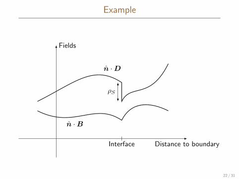
Example

Distance to boundary

Fields

Interface

n ·D

ρS

n ·B

22 / 31

Outline

1 Maxwell’s equations

2 Vector analysis

3 Boundary conditions

4 Conservation laws

5 Conclusions

23 / 31

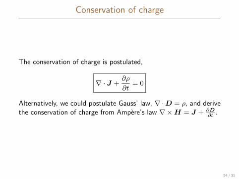
Conservation of charge

The conservation of charge is postulated,

∇ · J +∂ρ

∂t= 0

Alternatively, we could postulate Gauss’ law, ∇ ·D = ρ, and derivethe conservation of charge from Ampere’s law ∇×H = J + ∂D

∂t .

24 / 31

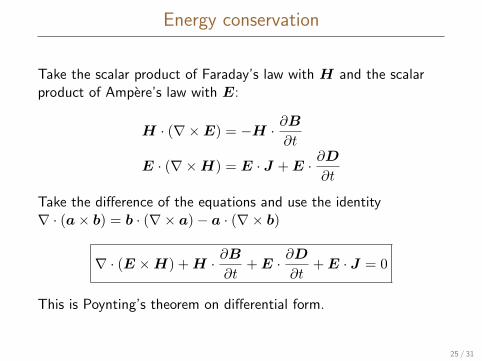
Energy conservation

Take the scalar product of Faraday’s law with H and the scalarproduct of Ampere’s law with E:

H · (∇×E) = −H · ∂B∂t

E · (∇×H) = E · J +E · ∂D∂t

Take the difference of the equations and use the identity∇ · (a× b) = b · (∇× a)− a · (∇× b)

∇ · (E ×H) +H · ∂B∂t

+E · ∂D∂t

+E · J = 0

This is Poynting’s theorem on differential form.

25 / 31

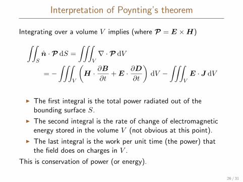
Interpretation of Poynting’s theorem

Integrating over a volume V implies (where P = E ×H)∫∫Sn ·P dS =

∫∫∫V∇ ·P dV

= −∫∫∫

V

(H · ∂B

∂t+E · ∂D

∂t

)dV −

∫∫∫VE · J dV

I The first integral is the total power radiated out of thebounding surface S.

I The second integral is the rate of change of electromagneticenergy stored in the volume V (not obvious at this point).

I The last integral is the work per unit time (the power) thatthe field does on charges in V .

This is conservation of power (or energy).

26 / 31

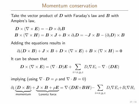
Momentum conservation

Take the vector product of D with Faraday’s law and B withAmpere’s law,

D × (∇×E) = −D × ∂tBB × (∇×H) = B × J +B × ∂tD = −J ×B − (∂tD)×B

Adding the equations results in

∂t(D ×B) + J ×B +D × (∇×E) +B × (∇×H) = 0

It can be shown that

D × (∇×E) = (∇ ·D)E +∑

i=x,y,z

Di∇Ei −∇ · (DE)

implying (using ∇ ·D = ρ and ∇ ·B = 0)

∂t (D ×B)︸ ︷︷ ︸momentum

+J ×B + ρE︸ ︷︷ ︸Lorentz force

= ∇·(DE+BH)−∑

i=x,y,z

Di∇Ei+Bi∇Hi

27 / 31

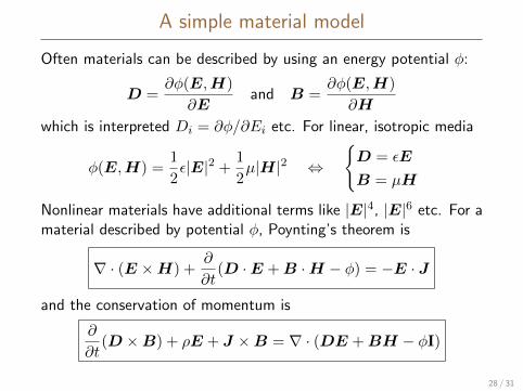
A simple material model

Often materials can be described by using an energy potential φ:

D =∂φ(E,H)

∂Eand B =

∂φ(E,H)

∂H

which is interpreted Di = ∂φ/∂Ei etc. For linear, isotropic media

φ(E,H) =1

2ε|E|2 + 1

2µ|H|2 ⇔

{D = εE

B = µH

Nonlinear materials have additional terms like |E|4, |E|6 etc. For amaterial described by potential φ, Poynting’s theorem is

∇ · (E ×H) +∂

∂t(D ·E +B ·H − φ) = −E · J

and the conservation of momentum is

∂

∂t(D ×B) + ρE + J ×B = ∇ · (DE +BH − φI)

28 / 31

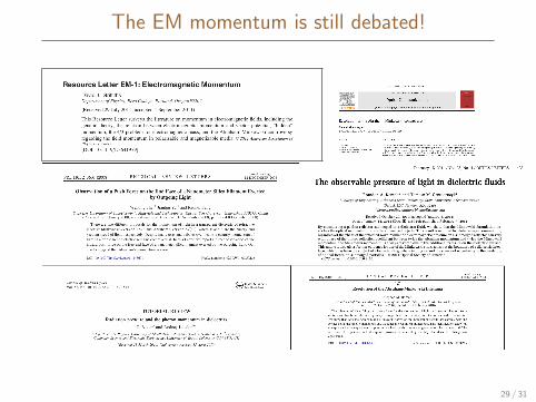
The EM momentum is still debated!

29 / 31

Outline

1 Maxwell’s equations

2 Vector analysis

3 Boundary conditions

4 Conservation laws

5 Conclusions

30 / 31

Conclusions

I Maxwell’s equations describe the dynamics of theelectromagnetic fields.

I Boundary conditions relate the values of the fields on differentsides of material boundaries to each other.

I Conservation laws can be derived to describe the conservationof physical entities such as power and momentum; these areusually products of two fields.

I Constitutive relations are necessary in order to fully solveMaxwell’s equations. Topic of next lecture!

31 / 31