electronic chip cooling in vertical configuration using...
TRANSCRIPT
1
ELECTRONIC CHIP COOLING IN VERTICALCONFIGURATION USING FLUENT-GAMBIT
A THESIS SUBMITTED IN PARTIAL FULFILLMENT OF THEREQUIREMENTS FOR THE DEGREE OF
Bachelor of Technology
in
Mechanical Engineering
By
PARESH RANJAN NAYAK
Department of Mechanical EngineeringNational Institute of Technology
Rourkela2007
2
ELECTRONIC CHIP COOLING IN VERTICALCONFIGURATION USING FLUENT-GAMBIT
A THESIS SUBMITTED IN PARTIAL FULFILLMENT OF THEREQUIREMENTS FOR THE DEGREE OF
Bachelor of Technology
in
Mechanical Engineering
By
PARESH RANJAN NAYAK
Under the guidance of
Dr. ASHOK KUMAR SATAPATHY
Department of Mechanical EngineeringNational Institute of Technology
Rourkela2007
3
National Institute of TechnologyRourkela
CERTIFICATE
This is to certify that the thesis entitled “ELECTRONIC CHIP COOLING IN
VERTICAL CONFIGURATION USING FLUENT GAMBIT” submitted by Sri Paresh
Ranjan Nayak in partial fulfillment of the requirements for the award of Bachelor of technology
Degree in Mechanical Engineering at the National Institute of Technology, Rourkela (Deemed
University) is an authentic work carried out by him under my supervision and guidance.
To the best of my knowledge, the matter embodied in the thesis has not been submitted to
any other University / Institute for the award of any Degree or Diploma.
Dr. Ashok Kumar Satapathy.National Institute of TechnologyRourkela-769008
Date

4
ACKNOWLEDGEMENT
We deem it a privilege to have been the student of Mechanical Engineering stream in
National Institute of Technology, ROURKELA
Our heartfelt thanks to Dr.A.K.Satapathy, our project guide who helped us to bring out
this project in good manner with his precious suggestion and rich experience.
We take this opportunity to express our sincere thanks to our project guide for co-
operation in accomplishing this project a satisfactory conclusion.
Paresh Ranjan NayakRoll No. 10303045Department of Mechanical EnggNational Institute of technology
5
CONTENTS
Contents .. i
Abstract ... ii
List of Figures . iii
1. Introduction
1.1 The miniaturization 2
1.2 CFD process 2
1.3 Cooling methods . 3
1.4 Thermal options for different packages........................................... 5
2. Theory2.1 Convection........................................................................................... 8
2.2 Reynolds Number................................................................................ 8
2.3 Nusselt Number................................................................................... 10
2.4 Prandtl Number.................................................................................. 11
2.5 Grashof Number.................................................................................. 12
2.6 Naviers-stoke equation........................................................................ 13
2.7 Discretization methods........................................................................ 14
3. About the project3.1 How does a CFD code work?.............................................................. 17
4. Fluent-Gambit analysis4.1 Design of 3-d channel using modeling tool gambit........................... 20
4.2 Fluent analysis..................................................................................... 22
5. Results and Discussions................................................................................ 28
6. Application of CFD....................................................................................... 39
7. Conclusion..................................................................................................... 40
Bibliography.................................................................................................. 41
i
6
ABSTRACT
In electronic equipments, thermal management is indispensable for its longevity and
hence it is once of the important topics of current research. These electronic equipments are
virtually synonyms with modern life, for instance appliances, instruments and computer
specifications. The dissipation of heat is necessary for its proper function. The heat is generated
by the resistance encountered by electric current. This has been further hastened by the continued
miniaturization of electronic systems which causes increase in the amount of heat generation per
unit volume by many folds. Unless proper cooling arrangement is designed, the operating
temperature exceeds permissible limit. As a consequence, chances of failure get increased. A
typical electronic system consists of several wire boards, known as printed circuit board (PCB),
on which large numbers of components are mounted. These PCBs are housed in an enclosure to
protect them from detrimental affect of environment, and also to protect users from electronic
hazards.
The enclosure has large number of vents on it to facilitate passage of cooling air. The
flow of air over the components is maintained either by fan or by free convection generated due
to heated components. The rate of the cooling of components strongly depends on the shape and
size of the enclosure, and also on the shape, size and location of vents. The objective of the
present study is to investigate the influences of these parameters on cooling of the components.
In this project, the heat and fluid characteristics of air in a vertical channel with multiple
square obstructions have been considered. The problem will be solved by using the software
package FLUENT – GAMBIT. The stream lines and will be plotted for visualization and to
study the heat transfer phenomena.
FLUENT is a computational fluid dynamics (CFD) software package to simulate fluid
flow problems. It uses the finite-volume method to solve the governing equations for a fluid. It
provides the capability to use different physical models such as incompressible or compressible,
iniviscid or viscous, laminar or turbulent, etc. Geometry and grid generation is done using
GAMBIT which is the preprocessor bundled with FLUENT.
ii
7
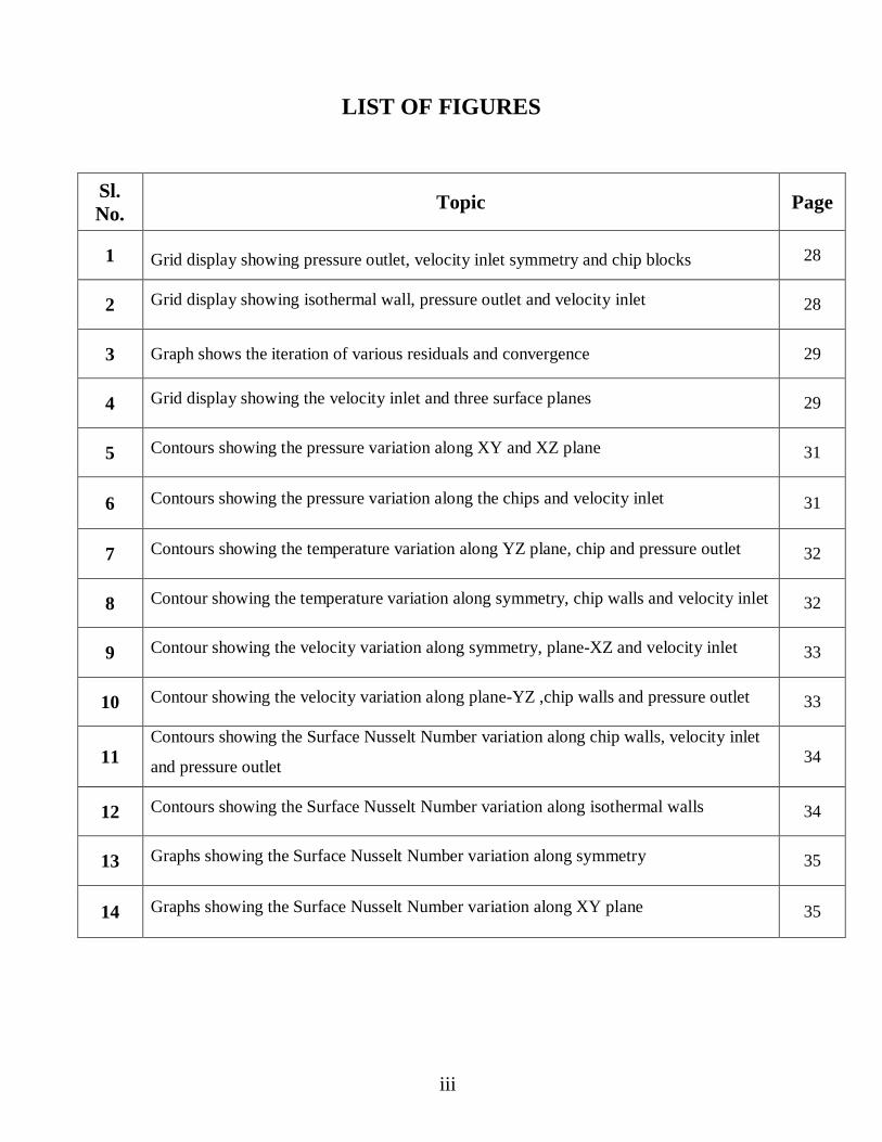
LIST OF FIGURES
Sl.No. Topic Page
1 Grid display showing pressure outlet, velocity inlet symmetry and chip blocks 28
2 Grid display showing isothermal wall, pressure outlet and velocity inlet 28
3 Graph shows the iteration of various residuals and convergence 29
4 Grid display showing the velocity inlet and three surface planes 29
5 Contours showing the pressure variation along XY and XZ plane 31
6 Contours showing the pressure variation along the chips and velocity inlet 31
7 Contours showing the temperature variation along YZ plane, chip and pressure outlet 32
8 Contour showing the temperature variation along symmetry, chip walls and velocity inlet 32
9 Contour showing the velocity variation along symmetry, plane-XZ and velocity inlet 33
10 Contour showing the velocity variation along plane-YZ ,chip walls and pressure outlet 33
11Contours showing the Surface Nusselt Number variation along chip walls, velocity inlet
and pressure outlet 34
12 Contours showing the Surface Nusselt Number variation along isothermal walls 34
13 Graphs showing the Surface Nusselt Number variation along symmetry 35
14 Graphs showing the Surface Nusselt Number variation along XY plane 35
iii

8
Chapter 1
INTRODUCTION
9
INTRODUCTION
1.1 THE MINIATURIZATION
From 1940, since the first electronic computers and devices were discovered, the
technology has come a long way. Faster and smaller computers have led to the development of
faster, denser and smaller circuit technologies which further has led to increased heat fluxes
generating at the chip and the package level. Over the years, significant advances have been
made in the application of air cooling techniques to manage increased heat fluxes. Air cooling
continues to be the most widely used method of cooling electronic components because this
method is easy to incorporate and is cheaply available. Although significant heat fluxes can be
accommodated with the use of liquid cooling, its use is still limited in most extreme cases where
there is no choice available.
FLUENT is a computational fluid dynamics (CFD) software package to simulate fluid
flow problems. It uses the finite-volume method to solve the governing equations for a fluid. It
provides the capability to use different physical models such as incompressible or compressible,
inviscid or viscous, laminar or turbulent, etc. Geometry and grid generation is done using
GAMBIT which is the preprocessor bundled with FLUENT.
1.2 CFD PROCESS:
Preprocessing is the first step in building and analyzing a flow model. It includes building
the model (or importing from a CAD package), applying the mesh, and entering the data. We
used Gambit as the preprocessing tool in our project.
There are four general purpose products: FLUENT, Flowizard, FIDAF, and
POLYFLOW. FLUENT is used in most industries All Fluent software includes full post
processing capabilities.
2
10
1.2.1 GAMBIT CFD PREPROCESSOR:
Fast geometry modeling and high quality meshing are crucial to successful use of
CFD.GAMBIT gives us both. Explore the advantage:
Ease of use
CAD/CAE Integration
Fast Modeling
CAD Cleanup
Intelligent Meshing
EASE-OF-USE
GAMBIT has a single interface for geometry creation and meshing that brings together
all of Fluent’s preprocessing technologies in one environment. Advanced tools for journaling let
us edit and conveniently replay model building sessions for parametric studies.
1.3 COOLING METHODS:
Various cooling methods are available for keeping electronic devices within their
operating temperature specifications.
1.3.2 VENTING
Natural air currents flow within any enclosure. Taking advantage of this current saves
on a long term component cost. Using a computer modeling package, a designer can experiment
with component placement and the addition of enclosure venting to determine an optimum
solution. When this solution fails to cool the device sufficiently, the addition of a fan is often
the next step.
1.3.3 ENCLOSURE FANS
The increased cooling provided by adding a fan to a system makes it a popular part of
many thermal solutions. Increased air flow also Increases the cooling efficiency of heat sinks,
allowing a smaller or less efficient heat sink to perform adequately.
The decision to add a fan to a system depends on number considerations. Mechanical
3
11
operation makes fans inherently less reliable than a passive system. In small enclosures, the
pressure drop between the inside and the outside of the enclosure can limit the efficiency of
the fan.
1.3.4 PASSIVE HEAT SINKS:
Passive heat sinks use a mass of thermally conductive material to move heat away from
the device into the air stream, where it can be carried away. Heat sink designs include fins or
other protrusions to increase the surface area, thus increasing its ability to remove heat from
the device.
1.3.5 ACTIVE HEAT SINKS:
When a passive heat sink cannot remove heat fast enough, a small fan may be added
directly to the heat sink itself, making the heat sink an active component. These active heat sinks,
often used to cool microprocessors, provide a dedicated air stream for a critical device. Active
heat sinks often are a good choice when an enclosure fan is impractical.
1.3.6 HEAT PIPES:
Heat pipes, a type of phase-change recalculating system, use the cooling power of
vaporization to move heat from one place to another. Within a closed heat removal system, such
as a sealed copper pipe, a fluid at the hot end (near a device) is changed into a vapor. Then the
gas passes through a heat removal area, typically a heat removal area, typically a heat sink using
either air cooling or liquid co04ng techniques. The temperature reduction causes the fluid to
recon dense into a liquid, giving off its heat to the environment. A heat pipe is a cost effective
solution, and it spreads the heat uniformly throughout the heat sink condenser section, increasing
its thermal effectiveness.
1.3.7 METAL BACKPLANES:
Metal-core primed circuit boards, stamped plates on the underside, of a laptop keyboard,
and large copper pads on the surface of a printed circuit board all employ large metallic areas to
dissipate heat.
4
12
1.3.8 THERMAL INTERFACES:
The interface between the device and the thermal product used to cool it is an important
factor in the thermal solution. For example, a heat sink attached to a plastic package using double
sided tape cannot dissipate the same amount of heat as the same heat sink directly in contain with
thermal transfer plate on a similar package.
Microscopic air gaps between a semiconductor package and the heat sink, caused by
surface non-uniformity, can degrade thermal performance. This degradation increases at
higher operating temperature. Interface materials appropriate to the package type reduce the
variability induced by varying surface roughness.
Since the interface thermal resistance is dependent upon allied force, the contact
pressure becomes an integral design parameter of the thermal solution. If a package/ device
can withstand a limited amount of contact pressure, it is important that thermal calculations
use the appropriate thermal resistance for that pressure.
The chemical compatibility of the interface materials with the package type is another
important factor.
1.4 THERMAL OPTIONS FOR DIFFERENT PACKAGES:Many applications have different constraints that favor one thermal solution over
another. Power devices need to dissipate large amount of heat. The thermal solution for
microprocessors must take space constraints into account. Surface mount and ball grid array
technologies have assembly considerations. Notebook computers require efficiency in every
area, including space, weight, and energy usage. While the optimum solution for anyone of
these package types must be determined on a case-by case basis, some solutions address
specific issues, making them more suitable for a particular application.
1.4.1 POWER DEVICES: Newer power devices incorporate surface mount compatibility into the power-hungry
design. These devices incorporate a heat transfer plate on the bottom of the device, which can
be wave soldered directly to the printed circuit board.
Metal-core substrates offer a potential solution to power device cooling, provided there are no
other heat-sensitive devices in the assembly, and the cost of the board can be justified.
5
13
1.4.2 MICROPROCESSORS:As microprocessor technology advances, the system designer struggles to keep
ahead of the increase in the thermal output of both (the voltage regulator and the
microprocessor. The use of active heat sinks allows concentrated, dedicated cooling of the
microprocessor, without severely impacting space requirements. For some applications,
specially designed passive heat sinks facilitate the use of higher-powered voltage regulators
in the same footprint, eliminating the need for board redesign.
1.4.3 BGAs:While BGA-packaged devices transfer more heat to the board then leaded devices,
the type of package can affect the ability to dissipate sufficient heat to maintain high device
reliability.
All plastic packages insulate the top of the device making heat dissipation through top
mounted heat sinks difficult and more expensive. Metal heat spreaders incorporated into the
top of the package enhance the ability to dissipate power from the chip
For some lower power devices flexible copper spreaders attach to pre-applied double
sided tape, offering a “quick-fix” for border line applications
As the need to dissipate more power increases, the optimum heat sink becomes
heavier. To prevent premature failure caused by ball shear, well designed of the self heat
sinks include spring loaded pins or clips that allow the weight of the heat sinks to be burn by
the PC-board instead of the device.
6

14
Chapter 2
THEORY
15
THEORY
2.1 CONVECTION
Convection in the most general terms refers to the internal movement of currents within
fluids (i.e. liquids and gases). It cannot occur in solids due to the atoms not being able to flow
freely.
Convection may cause a related phenomenon called advection, in which either mass or
heat is transported by the currents or motion in the fluid.A common use of the term convection
relates to the special case in which advected (carried) substance is heat. In this case, the heat
itself may be an indirect cause of the fluid motion even while being transported by it. In this
case, the problem of heat transport (and related transport of other substances in the fluid due to
it) may become especially complicated.
Convection is of two types:-
1. Forced convection
2. Free Convetion
Forced Convection: When the density difference is created by some means like blower or
compressor and due to which circulation takes place then it is know as forced convection
Free Convection: Density variation happens naturally then it is called free convection
Here we are concerned for Newtonian fluid only(fluid that follows Newton law of cooling)
yu
∂∂
= µτ
2.2 REYNOLDS NUMBER
In fluid mechanics, the Reynolds number is the ratio of inertial forces (vs ) to viscous
forces ( /L) and consequently it quantifies the relative importance of these two types of forces
for given flow conditions. Thus, it is used to identify different flow regimes, such as laminar or
turbulent flow.
8
16
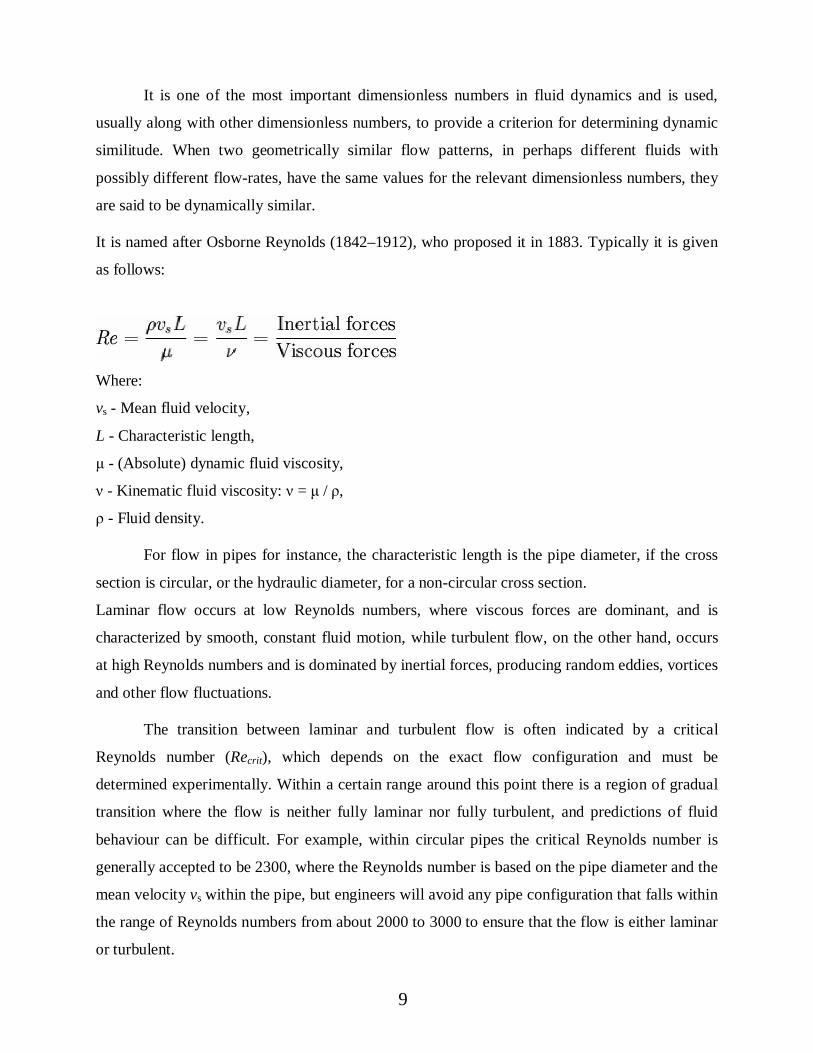
It is one of the most important dimensionless numbers in fluid dynamics and is used,
usually along with other dimensionless numbers, to provide a criterion for determining dynamic
similitude. When two geometrically similar flow patterns, in perhaps different fluids with
possibly different flow-rates, have the same values for the relevant dimensionless numbers, they
are said to be dynamically similar.
It is named after Osborne Reynolds (1842–1912), who proposed it in 1883. Typically it is given
as follows:
Where:
vs - Mean fluid velocity,
L - Characteristic length,
- (Absolute) dynamic fluid viscosity,
- Kinematic fluid viscosity: = / ,
- Fluid density.
For flow in pipes for instance, the characteristic length is the pipe diameter, if the cross
section is circular, or the hydraulic diameter, for a non-circular cross section.
Laminar flow occurs at low Reynolds numbers, where viscous forces are dominant, and is
characterized by smooth, constant fluid motion, while turbulent flow, on the other hand, occurs
at high Reynolds numbers and is dominated by inertial forces, producing random eddies, vortices
and other flow fluctuations.
The transition between laminar and turbulent flow is often indicated by a critical
Reynolds number (Recrit), which depends on the exact flow configuration and must be
determined experimentally. Within a certain range around this point there is a region of gradual
transition where the flow is neither fully laminar nor fully turbulent, and predictions of fluid
behaviour can be difficult. For example, within circular pipes the critical Reynolds number is
generally accepted to be 2300, where the Reynolds number is based on the pipe diameter and the
mean velocity vs within the pipe, but engineers will avoid any pipe configuration that falls within
the range of Reynolds numbers from about 2000 to 3000 to ensure that the flow is either laminar
or turbulent.
9
17
For flow over a flat plate, the characteristic length is the length of the plate and the
characteristic velocity is the free stream velocity. In a boundary layer over a flat plate the local
regime of the flow is determined by the Reynolds number based on the distance measured from
the leading edge of the plate. In this case, the transition to turbulent flow occurs at a Reynolds
number of the order of 105 or 106.
2.3 NUSSELT NUMBER
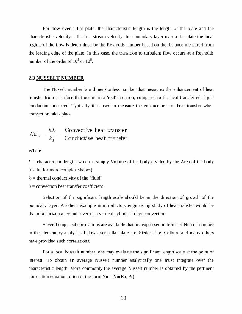
The Nusselt number is a dimensionless number that measures the enhancement of heat
transfer from a surface that occurs in a 'real' situation, compared to the heat transferred if just
conduction occurred. Typically it is used to measure the enhancement of heat transfer when
convection takes place.
Where
L = characteristic length, which is simply Volume of the body divided by the Area of the body
(useful for more complex shapes)
kf = thermal conductivity of the "fluid"
h = convection heat transfer coefficient
Selection of the significant length scale should be in the direction of growth of the
boundary layer. A salient example in introductory engineering study of heat transfer would be
that of a horizontal cylinder versus a vertical cylinder in free convection.
Several empirical correlations are available that are expressed in terms of Nusselt number
in the elementary analysis of flow over a flat plate etc. Sieder-Tate, Colburn and many others
have provided such correlations.
For a local Nusselt number, one may evaluate the significant length scale at the point of
interest. To obtain an average Nusselt number analytically one must integrate over the
characteristic length. More commonly the average Nusselt number is obtained by the pertinent
correlation equation, often of the form Nu = Nu(Ra, Pr).
10
18
The Nusselt number can also be viewed as being a dimensionless temperature gradient at the
surface.
2.4 PRANDTL NUMBER
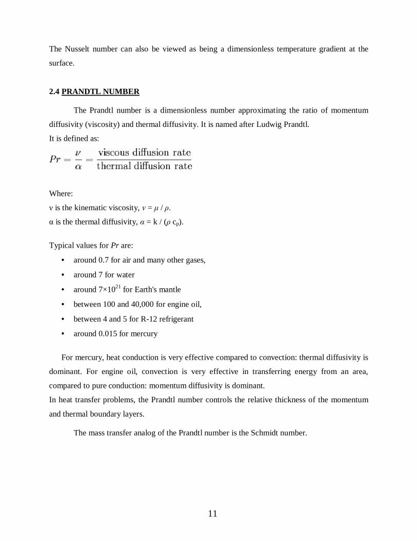
The Prandtl number is a dimensionless number approximating the ratio of momentum
diffusivity (viscosity) and thermal diffusivity. It is named after Ludwig Prandtl.
It is defined as:
Where:
is the kinematic viscosity, = / .
is the thermal diffusivity, = k / ( cp).
Typical values for Pr are:
• around 0.7 for air and many other gases,
• around 7 for water
• around 7×10²¹ for Earth's mantle
• between 100 and 40,000 for engine oil,
• between 4 and 5 for R-12 refrigerant
• around 0.015 for mercury
For mercury, heat conduction is very effective compared to convection: thermal diffusivity is
dominant. For engine oil, convection is very effective in transferring energy from an area,
compared to pure conduction: momentum diffusivity is dominant.
In heat transfer problems, the Prandtl number controls the relative thickness of the momentum
and thermal boundary layers.
The mass transfer analog of the Prandtl number is the Schmidt number.
11
19
2.5 GRASHOF NUMBER
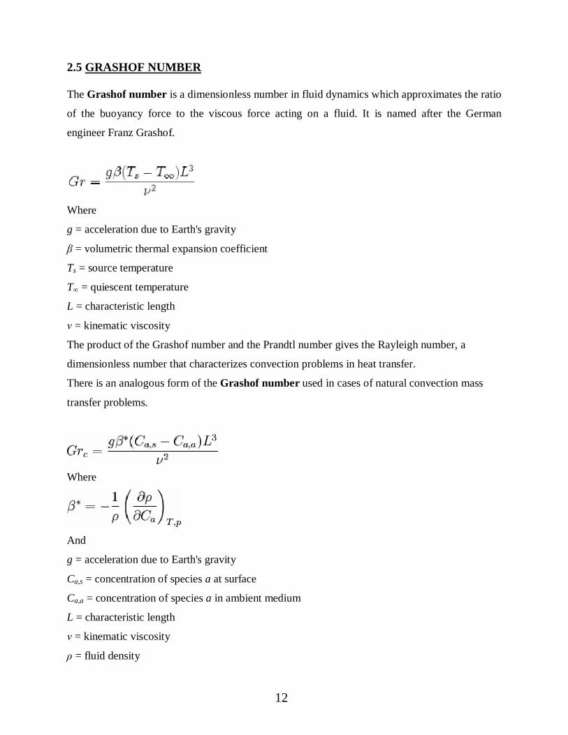
The Grashof number is a dimensionless number in fluid dynamics which approximates the ratio
of the buoyancy force to the viscous force acting on a fluid. It is named after the German
engineer Franz Grashof.
Where
g = acceleration due to Earth's gravity
= volumetric thermal expansion coefficient
Ts = source temperature
T = quiescent temperature
L = characteristic length
= kinematic viscosity
The product of the Grashof number and the Prandtl number gives the Rayleigh number, a
dimensionless number that characterizes convection problems in heat transfer.
There is an analogous form of the Grashof number used in cases of natural convection mass
transfer problems.
Where
And
g = acceleration due to Earth's gravity
Ca,s = concentration of species a at surface
Ca,a = concentration of species a in ambient medium
L = characteristic length
= kinematic viscosity
= fluid density
12
20
Ca = concentration of species a
T = constant temperature
p = constant pressure
2.6 NAVIER-STOKES EQUATION
The Navier-Stokes equations are derived from conservation principles of:
• Mass
• Energy
• Momentum
• Angular momentum
• Equation of continuity
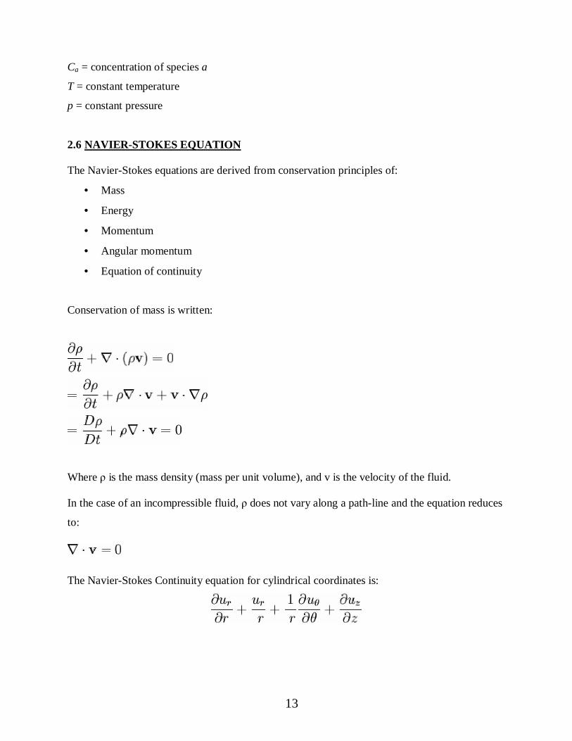
Conservation of mass is written:
Where is the mass density (mass per unit volume), and v is the velocity of the fluid.
In the case of an incompressible fluid, does not vary along a path-line and the equation reduces
to:
The Navier-Stokes Continuity equation for cylindrical coordinates is:
13
21
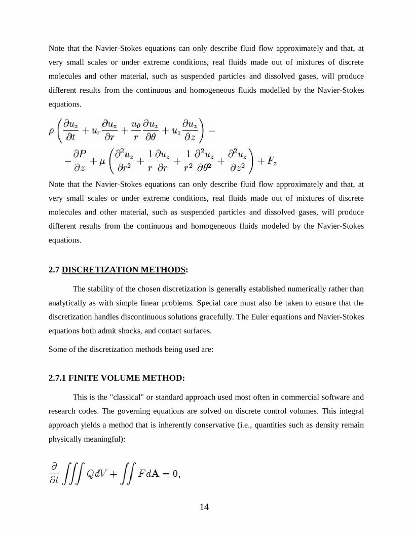
Note that the Navier-Stokes equations can only describe fluid flow approximately and that, at
very small scales or under extreme conditions, real fluids made out of mixtures of discrete
molecules and other material, such as suspended particles and dissolved gases, will produce
different results from the continuous and homogeneous fluids modelled by the Navier-Stokes
equations.
Note that the Navier-Stokes equations can only describe fluid flow approximately and that, at
very small scales or under extreme conditions, real fluids made out of mixtures of discrete
molecules and other material, such as suspended particles and dissolved gases, will produce
different results from the continuous and homogeneous fluids modeled by the Navier-Stokes
equations.
2.7 DISCRETIZATION METHODS:
The stability of the chosen discretization is generally established numerically rather than
analytically as with simple linear problems. Special care must also be taken to ensure that the
discretization handles discontinuous solutions gracefully. The Euler equations and Navier-Stokes
equations both admit shocks, and contact surfaces.
Some of the discretization methods being used are:
2.7.1 FINITE VOLUME METHOD:
This is the "classical" or standard approach used most often in commercial software and
research codes. The governing equations are solved on discrete control volumes. This integral
approach yields a method that is inherently conservative (i.e., quantities such as density remain
physically meaningful):
14
22
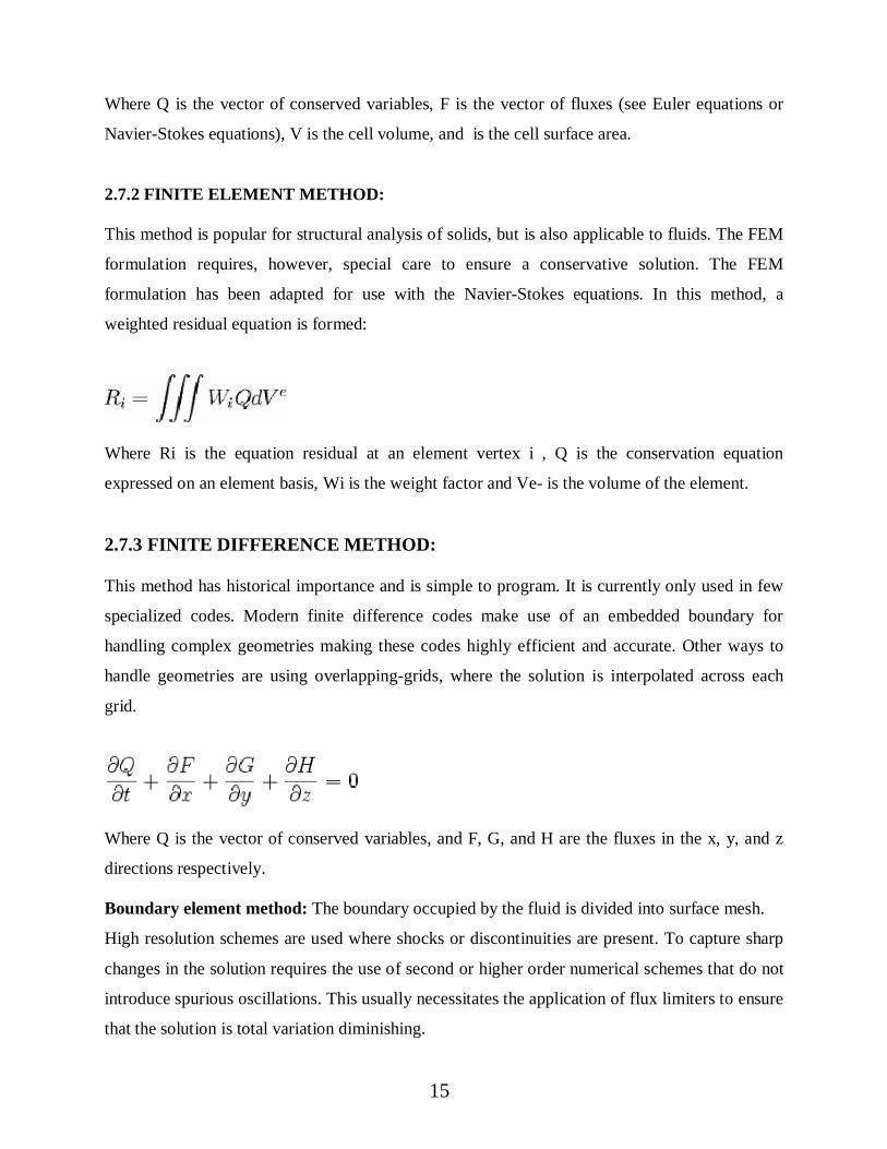
Where Q is the vector of conserved variables, F is the vector of fluxes (see Euler equations or
Navier-Stokes equations), V is the cell volume, and is the cell surface area.
2.7.2 FINITE ELEMENT METHOD:
This method is popular for structural analysis of solids, but is also applicable to fluids. The FEM
formulation requires, however, special care to ensure a conservative solution. The FEM
formulation has been adapted for use with the Navier-Stokes equations. In this method, a
weighted residual equation is formed:
Where Ri is the equation residual at an element vertex i , Q is the conservation equation
expressed on an element basis, Wi is the weight factor and Ve- is the volume of the element.
2.7.3 FINITE DIFFERENCE METHOD:
This method has historical importance and is simple to program. It is currently only used in few
specialized codes. Modern finite difference codes make use of an embedded boundary for
handling complex geometries making these codes highly efficient and accurate. Other ways to
handle geometries are using overlapping-grids, where the solution is interpolated across each
grid.
Where Q is the vector of conserved variables, and F, G, and H are the fluxes in the x, y, and z
directions respectively.
Boundary element method: The boundary occupied by the fluid is divided into surface mesh.
High resolution schemes are used where shocks or discontinuities are present. To capture sharp
changes in the solution requires the use of second or higher order numerical schemes that do not
introduce spurious oscillations. This usually necessitates the application of flux limiters to ensure
that the solution is total variation diminishing.
15

23
Chapter 3
ABOUT THE PROJECT
24
ABOUT THE PROJECT
In this project, the heat and fluid characteristics of air in a vertical channel with multiple
square obstructions have been considered. The problem will be solved using FLUENT-GAMBIT
software package which have FLUENT 6.0 and GAMBIT 2.0 bundled into one package to solve
CFD problems. GAMBIT is used to create the initial geometry and meshing. FLUENT is used to
analyze and solve the geometry with the boundary conditions and specifications mentioned.
Different layouts of multiple square obstructions will be considered including a parallel
layout and a zigzag configuration. The heat transfer in each case will be calculated and the
configuration having maximum beat transfer rate will be the optimal one and will be used for
future considerations. The isotherms and streamlines will be plotted for Bow visualization and to
study the heat transfer phenomena for this configuration. The distribution of temperature and
pressure of the fluid (air) along the chip face and wall are also analyzed.
The figure below shows two substrates having electronic chip arranged on them in a
zigzag fashion. Air flows from a fan in order to cool the chips the area of the chips is assumed to
be square type.
3.1 HOW DOES A CFD CODE WORK?
CFD codes are structured around the numerical algorithms that can be tackle fluid problems. In
order to provide easy access to their solving power all commercial CFD packages include
sophisticated user interfaces input problem parameters and to examine the results. Hence all
codes contain three main elements:
1. Pre-processing.
2. Solver
3. Post processing.
3.1.1 PRE-PROCESSING: Preprocessor consists of input of a flow problem by means of an
operator friendly interface and subsequent transformation of this input into form of suitable for
the use by the solver.
17
25
The user activities at the Pre-processing stage involve: Definition of the geometry of the region:
The computational domain. Grid generation is the subdivision of the domain into a number of
smaller, non-overlapping sub domains (or control volumes or elements Selection of physical or
chemical phenomena that need to be modeled).
Definition of fluid properties: Specification of appropriate boundary conditions at cells, which
coincide with or touch the boundary.
The solution of a flow problem (velocity, pressure, temperature etc.) is defined at odes
inside each cell. The accuracy of CFD solutions is governed by number of cells in the grid. In
general, the larger numbers of cells better the solution accuracy. Both the accuracy of the
solution & its cost in terms of necessary computer hardware & calculation time are dependent on
the fineness of the grid. Efforts are underway to develop CFD codes with a (self) adaptive
meshing capability. Ultimately such programs will automatically refine the grid in areas of rapid
variation.
3.1.2 SOLVER: These are three distinct streams of numerical solutions techniques: finite
difference, finite volume& finite element methods. In outline the numerical methods that form
the basis of solver performs the following steps
The approximation of unknown flow variables are by means of simple functions.
Discretization by substitution of the approximation into the governing flow equations &*
subsequent mathematical manipulations.
3.1.3 POST-PROCESSING: As in the pre-processing huge amount of development work has
recently has taken place in the post processing field. Owing to increased popularity of
engineering work stations, many of which has outstanding graphics capabilities, the leading CFD
are now equipped with versatile data visualization tools. These include
• Domain geometry & Grid display.
• Vector plots.
• Line & shaded contour plots.
• 2D & 3D surface plots.
• Particle tracking.
• View manipulation (translation, rotation, scaling etc.)
18

26
Chapter 4
FLUENT-GAMBIT ANALYSIS
27
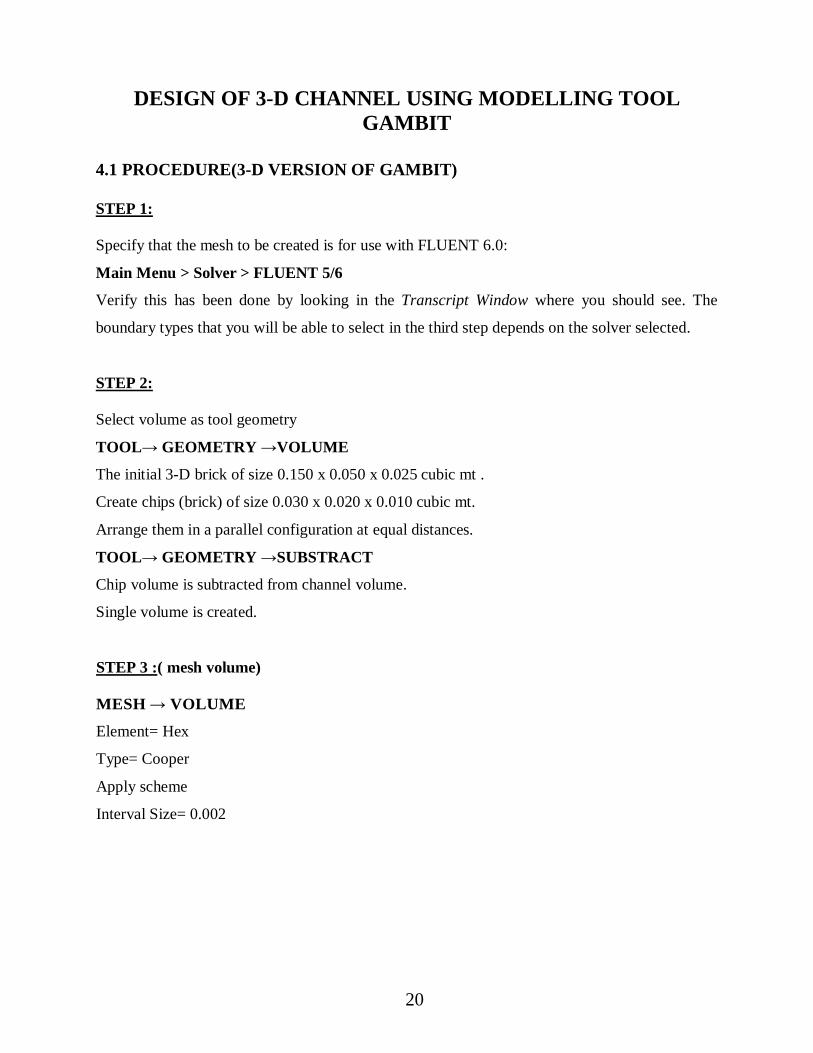
DESIGN OF 3-D CHANNEL USING MODELLING TOOLGAMBIT
4.1 PROCEDURE(3-D VERSION OF GAMBIT)
STEP 1:
Specify that the mesh to be created is for use with FLUENT 6.0:
Main Menu > Solver > FLUENT 5/6
Verify this has been done by looking in the Transcript Window where you should see. The
boundary types that you will be able to select in the third step depends on the solver selected.
STEP 2:
Select volume as tool geometry
TOOL GEOMETRY VOLUME
The initial 3-D brick of size 0.150 x 0.050 x 0.025 cubic mt .
Create chips (brick) of size 0.030 x 0.020 x 0.010 cubic mt.
Arrange them in a parallel configuration at equal distances.
TOOL GEOMETRY SUBSTRACT
Chip volume is subtracted from channel volume.
Single volume is created.
STEP 3 :( mesh volume)
MESH VOLUME
Element= Hex
Type= Cooper
Apply scheme
Interval Size= 0.002
20
28
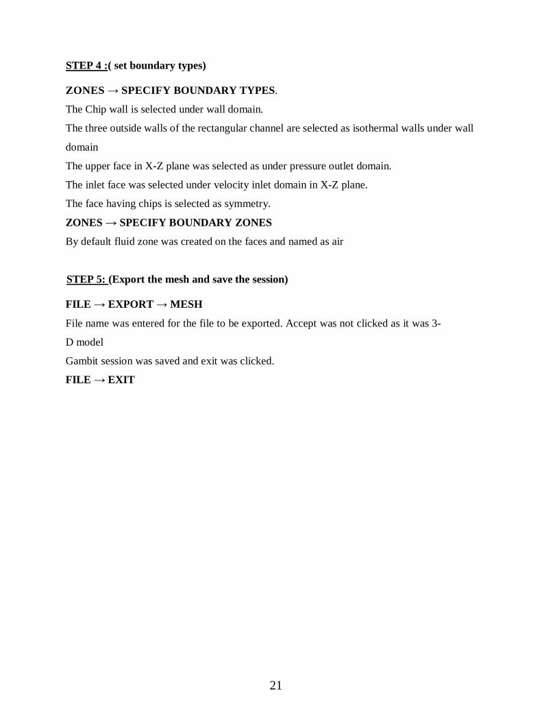
STEP 4 :( set boundary types)
ZONES SPECIFY BOUNDARY TYPES.
The Chip wall is selected under wall domain.
The three outside walls of the rectangular channel are selected as isothermal walls under wall
domain
The upper face in X-Z plane was selected as under pressure outlet domain.
The inlet face was selected under velocity inlet domain in X-Z plane.
The face having chips is selected as symmetry.
ZONES SPECIFY BOUNDARY ZONES
By default fluid zone was created on the faces and named as air
STEP 5: (Export the mesh and save the session)
FILE EXPORT MESH
File name was entered for the file to be exported. Accept was not clicked as it was 3-
D model
Gambit session was saved and exit was clicked.
FILE EXIT
21

29
4.2 ANALYSIS IN FLUENT
PROCEDURE: (3D VERSION OF FLUENT)
STEP 1: (GRID)
FILE READ CASE
The file channel mesh is selected by clicking on it under files and
Then ok is clicked.
The grid is checked.
GRID CHECK
The grid was scaled to 1 in all x, y and z directions.
GRID SCALE
The grid was displayed.
DISPLAY GRID
Grid is copied in ms-word file.
STEP 2 :( Models)
The solver was specified.
DEFINE MODELS SOLVER
Solver is segregated
Implicit formulation
Space steady
Time steady
DEFINE MODEL ENERGY
Energy equation is clicked on.
DEFINE MODELS VISCOUS
The standard k- turbulence model was turned on.
k- model(2-equation)- Standard
Model constants
Cmu-0.09
C1-Epsilon-1.44
22
30
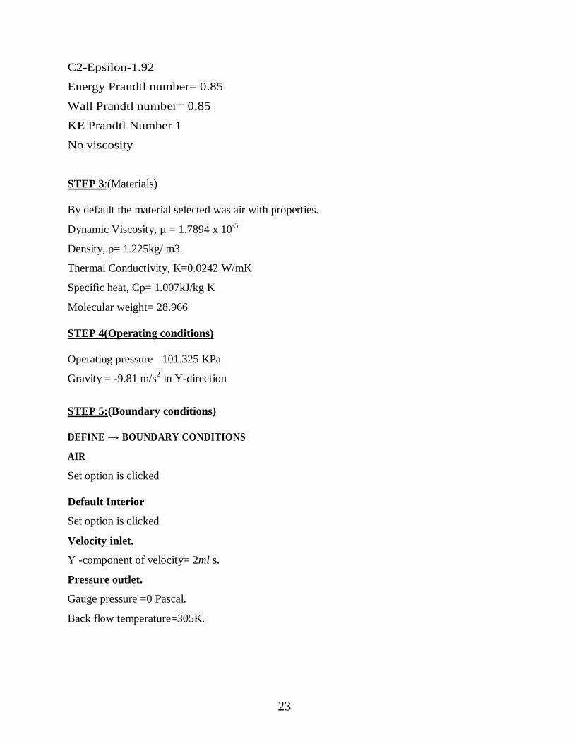
C2-Epsilon-1.92
Energy Prandtl number= 0.85
Wall Prandtl number= 0.85
KE Prandtl Number 1
No viscosity
STEP 3:(Materials)
By default the material selected was air with properties.
Dynamic Viscosity, µ = 1.7894 x 10⁻⁵
Density, = 1.225kg/ m3.
Thermal Conductivity, K=0.0242 W/mK
Specific heat, Cp= 1.007kJ/kg K
Molecular weight= 28.966
STEP 4(Operating conditions)
Operating pressure= 101.325 KPa
Gravity = -9.81 m/s2 in Y-direction
STEP 5:(Boundary conditions)
DEFINE BOUNDARY CONDITIONS
AIR
Set option is clicked
Default Interior
Set option is clicked
Velocity inlet.
Y -component of velocity= 2ml s.
Pressure outlet.
Gauge pressure =0 Pascal.
Back flow temperature=305K.
23
31
Wall 1 (Isothermal Wall)-Channel Wall
Temperature= 350K
Wall thickness=0mm.
Material= Aluminium
Wall 2 (Constant heat flux generation)-Chip Wall
Constant Heat Flux, W= 1000W/m2
Wall thickness=0mm.
Material= Aluminium
STEP 6: (Solution)
SOLVE CONTROLS SOLUTIONS
All flow, turbulent and energy equation used.
Under relaxation factors
Pressure= 0.3
Density= 1
Body Force= 1
Momentum= 0.08
SOLVE INTIALIZE
Compute from velocity inlet= 2m/s
Click INIT
~Velocity inlet was chosen from the computer from the list.
~ X component of velocity is 0.
~ Init was clicked and panel was closed.
The plotting of residuals was enabled for the calculation.
PLOT RESIDUALS
Plot option was clicked than ok was clicked.
The case file was created
FILE WRITE- CASE
The calculation was started by requesting 1000 iterations
SOLVE ITERATE
Input 100 as the number of iterations and iterate was clicked.
Convergence was checked.
24
32
Converged in 52 iterations
REPORT FLUXES
Mass flow rate
Total heat transfer
Radiation heat transfer
Their values along all zones are computed
The data was saved.
FILE WRITE DATA
Arbitrary planes were created along XYZ Cartesian coordinate system for contour evaluation for
flow inside the channel.
STEP 6:(Displaying the preliminary solution)
Display of filled contours of velocity magnitude
DISPLAY CONTOURS
~ Velocity was selected and then velocity magnitude in the
Drop down list was selected.
~filled under option was selected.
~Display was clicked.
Display of filled contours of temperature
DISPLAY CONTOURS
~Temperature was selected and then
1. Static temperature.
2. Total temperature from drop down list was selected
~Display was clicked.
Display of filled contours of turbulence
DISPLAY CONTOURS
~ Turbulence was selected along various planes
~filled under option was selected.
~Display was clicked.
Display of filled contours of wall fluxes
DISPLAY CONTOURS
25
33
~ Wall fluxes was selected and then suface nusselt number in the
Drop down list was selected.
~filled under option was selected.
~Display was clicked.
Display velocity vector.
DISPLAY VECTOR
~Display was clicked to plot the velocity vectors.
An XY plot of temperature across the exit was created.
PLOT XY PLOT
~ Wall fluxes were selected and Surface Nusselt in the drop down list under the Y axis
functions.
The write option is clicked to save data in ms-excel file. It contains surface Nusselt number
values with there node points.
The excel file is opened and we plot a graph of surface Nusselt number along Y-axis and
position on Y-axis in grid display in meter along X-axis.
The graph we plot is along XZ plane and symmetry
~ Plot was clicked.
~ The average value of surface Nusselt along these two planes is calculated as 189 and 210
Similarly, We write the data of surface Nusselt along all node points including all zones in ms-
excel file and calculate average surface Nusselt number. The value was found out to be 214
CALCULATION OF REYNOLDS NUMBER
= (1.225 x 2 x 0.035) / (1.7894x10⁻⁵)
= 4792.11 [Hence the flow is turbulent (Rectangular channel flow)]
After doing many simulations with varying mesh element, type and spacing between the grids
the values of surface Nusselt number was found to be same on average hence through grid
independence check our simulation values are found to be correct.
The graphs and contours related to CFD analysis done above is shown from next page.
26

34
Chapter 5
DISCUSSION
35
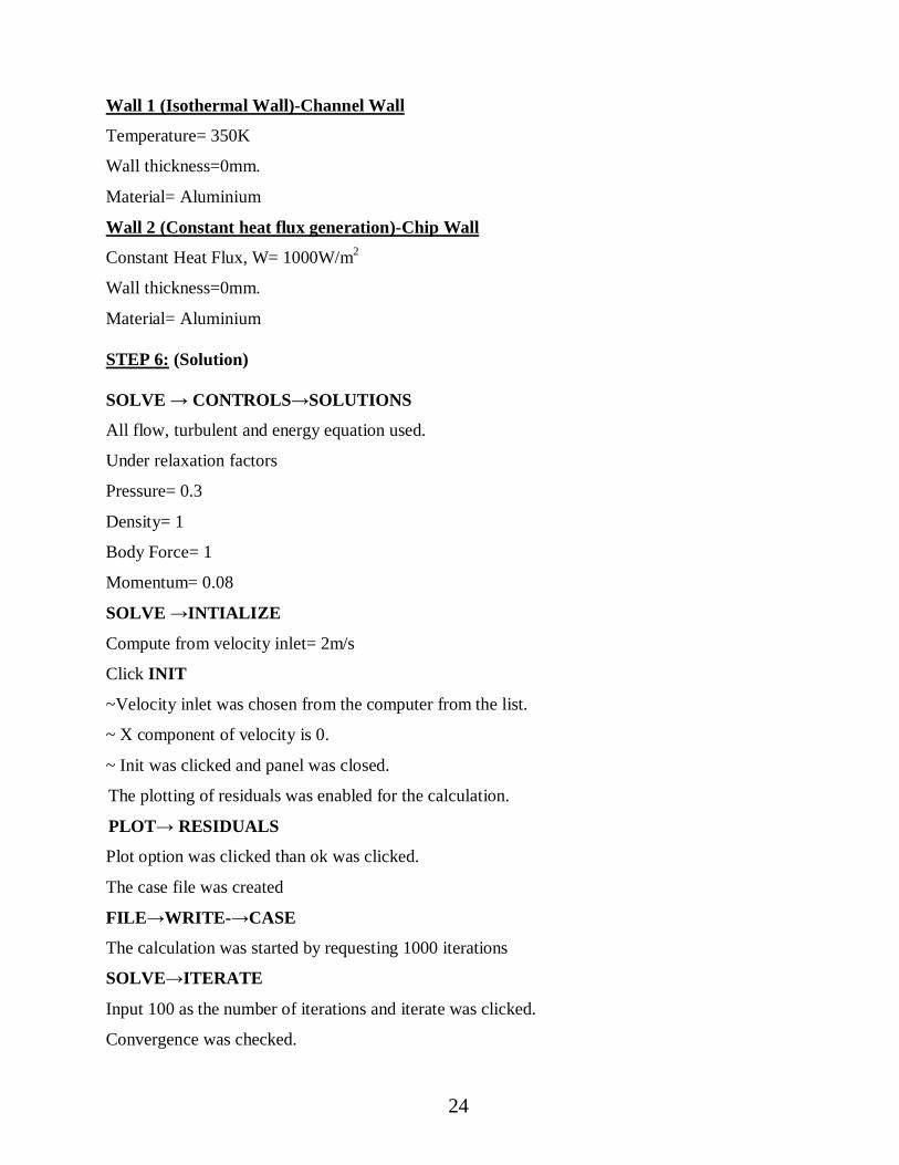
Fig 5.1 Grid display showing pressure outlet, velocity inlet symmetry and chip blocks
GRID DISPLAY
28
36
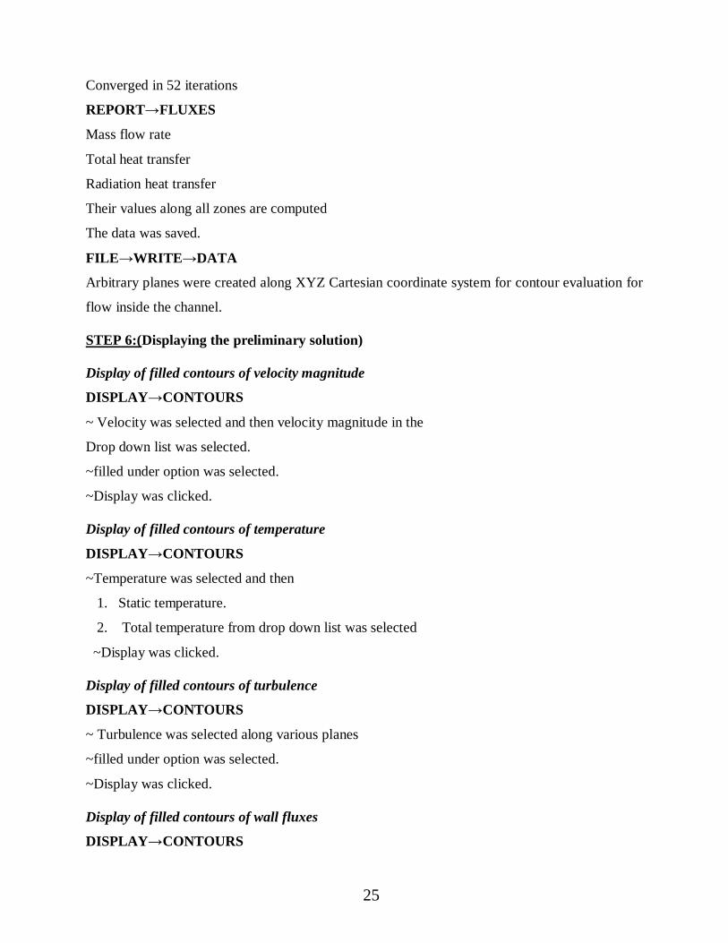
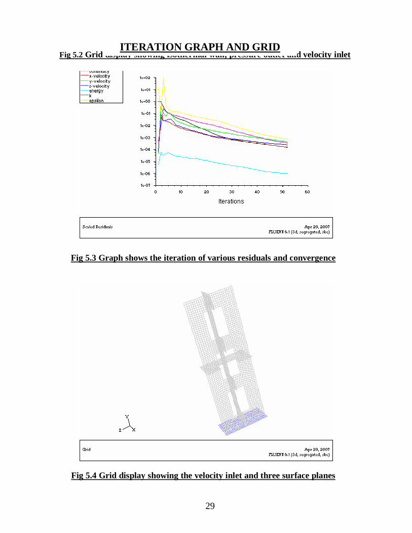
Fig 5.2 Grid display showing isothermal wall, pressure outlet and velocity inletITERATION GRAPH AND GRID
Fig 5.3 Graph shows the iteration of various residuals and convergence
Fig 5.4 Grid display showing the velocity inlet and three surface planes
29
37
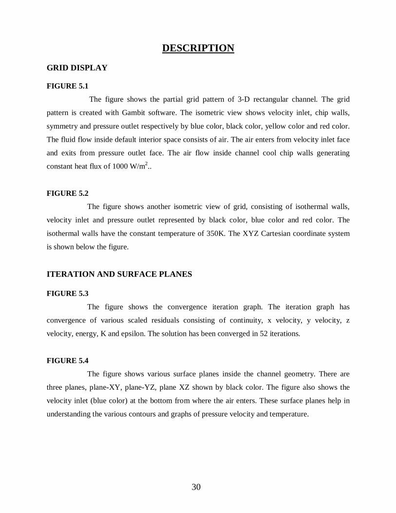
DESCRIPTION
GRID DISPLAY
FIGURE 5.1
The figure shows the partial grid pattern of 3-D rectangular channel. The grid
pattern is created with Gambit software. The isometric view shows velocity inlet, chip walls,
symmetry and pressure outlet respectively by blue color, black color, yellow color and red color.
The fluid flow inside default interior space consists of air. The air enters from velocity inlet face
and exits from pressure outlet face. The air flow inside channel cool chip walls generating
constant heat flux of 1000 W/m2..
FIGURE 5.2
The figure shows another isometric view of grid, consisting of isothermal walls,
velocity inlet and pressure outlet represented by black color, blue color and red color. The
isothermal walls have the constant temperature of 350K. The XYZ Cartesian coordinate system
is shown below the figure.
ITERATION AND SURFACE PLANES
FIGURE 5.3
The figure shows the convergence iteration graph. The iteration graph has
convergence of various scaled residuals consisting of continuity, x velocity, y velocity, z
velocity, energy, K and epsilon. The solution has been converged in 52 iterations.
FIGURE 5.4
The figure shows various surface planes inside the channel geometry. There are
three planes, plane-XY, plane-YZ, plane XZ shown by black color. The figure also shows the
velocity inlet (blue color) at the bottom from where the air enters. These surface planes help in
understanding the various contours and graphs of pressure velocity and temperature.
30
38
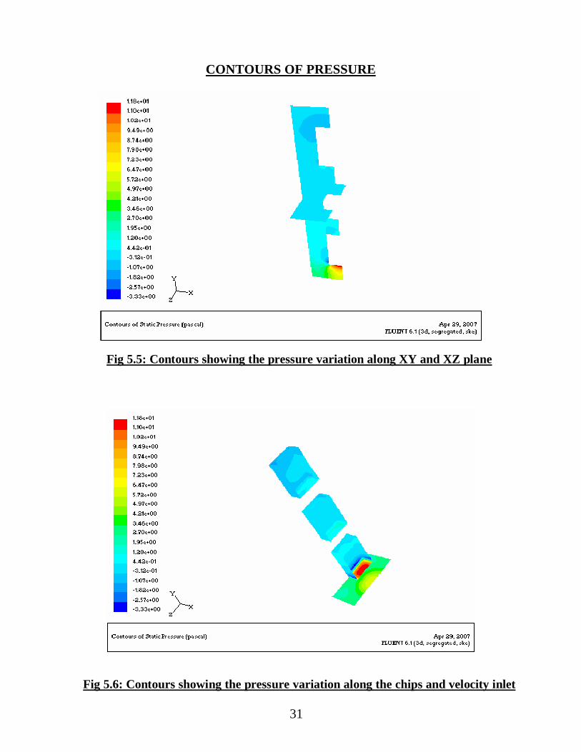
CONTOURS OF PRESSURE
Fig 5.5: Contours showing the pressure variation along XY and XZ plane
Fig 5.6: Contours showing the pressure variation along the chips and velocity inlet
31
39
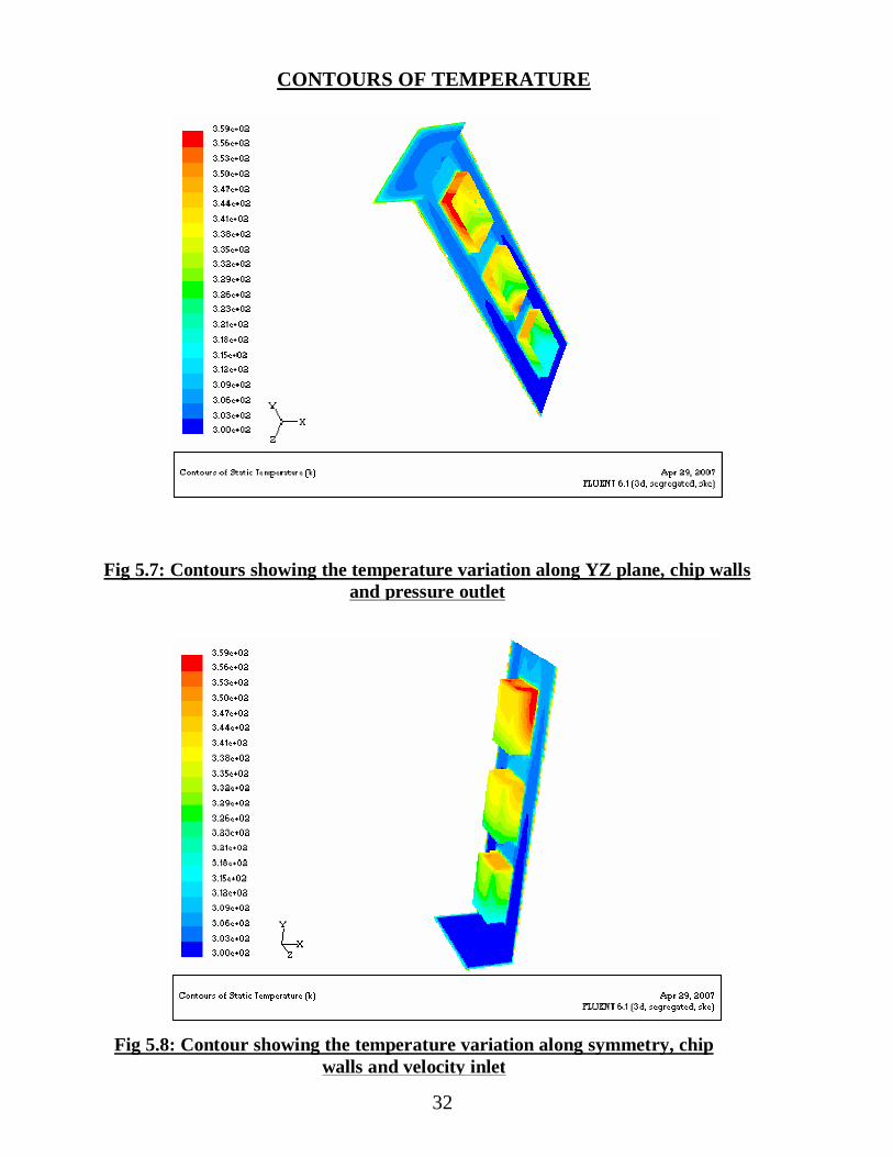
Fig 5.7: Contours showing the temperature variation along YZ plane, chip wallsand pressure outlet
Fig 5.8: Contour showing the temperature variation along symmetry, chipwalls and velocity inlet
CONTOURS OF TEMPERATURE
32
40
CONTOURS OF SURFACE NUSSELT NUMBERFig 5.10: Contour showing the velocity variation along plane-YZ ,chip walls
and pressure outlet
Fig 5.9: Contour showing the velocity variation along symmetry, plane-XZand velocity inlet
CONTOURS OF VELOCITY
33
41
GRAPHS OF SURFACE NUSSELT NUMBERFig 5.12: Contours showing the Surface Nusselt Number variation alongisothermal walls
Fig 5.11: Contours showing the Surface Nusselt Number variation alongchip walls, velocity inlet and pressure outlet
CONTOURS OF SURFACE NUSSELT NUMBER
34
42
surface nusselt along symmetry
0200400600800
100012001400160018002000
0 0.05 0.1 0.15 0.2
position along y-axis in m
surfa
ce n
usse
lt nu
mbe
r
Series1
surface nusselt number along XY-axis
0200400600800
100012001400160018002000
0 0.05 0.1 0.15 0.2
position along Y-axis in m
surfa
ce n
usse
lt nu
mbe
r
Series1
DISCUSSION
Fig 5.13 Graphs showing the Surface Nusselt Number variation along symmetry
Fig 5.14 Graphs showing the Surface Nusselt Number variation along XY plane
GRAPHS OF SURFACE NUSSELT NUMBER
35
43
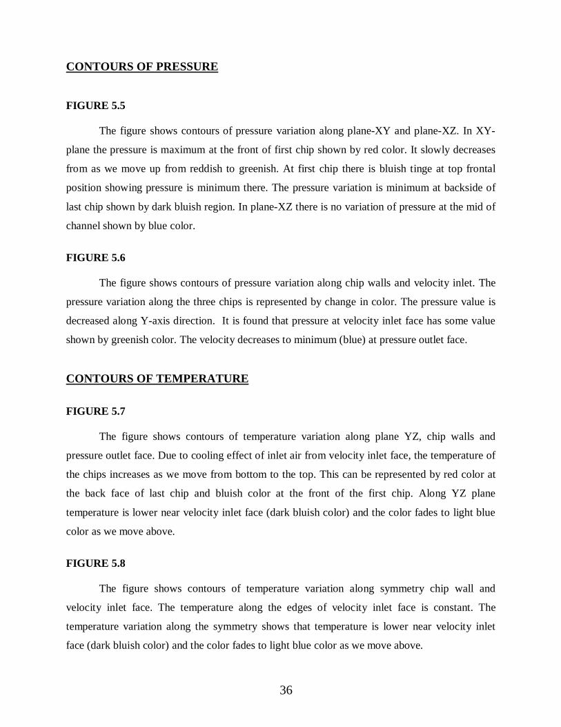
CONTOURS OF PRESSURE
FIGURE 5.5
The figure shows contours of pressure variation along plane-XY and plane-XZ. In XY-
plane the pressure is maximum at the front of first chip shown by red color. It slowly decreases
from as we move up from reddish to greenish. At first chip there is bluish tinge at top frontal
position showing pressure is minimum there. The pressure variation is minimum at backside of
last chip shown by dark bluish region. In plane-XZ there is no variation of pressure at the mid of
channel shown by blue color.
FIGURE 5.6
The figure shows contours of pressure variation along chip walls and velocity inlet. The
pressure variation along the three chips is represented by change in color. The pressure value is
decreased along Y-axis direction. It is found that pressure at velocity inlet face has some value
shown by greenish color. The velocity decreases to minimum (blue) at pressure outlet face.
CONTOURS OF TEMPERATURE
FIGURE 5.7
The figure shows contours of temperature variation along plane YZ, chip walls and
pressure outlet face. Due to cooling effect of inlet air from velocity inlet face, the temperature of
the chips increases as we move from bottom to the top. This can be represented by red color at
the back face of last chip and bluish color at the front of the first chip. Along YZ plane
temperature is lower near velocity inlet face (dark bluish color) and the color fades to light blue
color as we move above.
FIGURE 5.8
The figure shows contours of temperature variation along symmetry chip wall and
velocity inlet face. The temperature along the edges of velocity inlet face is constant. The
temperature variation along the symmetry shows that temperature is lower near velocity inlet
face (dark bluish color) and the color fades to light blue color as we move above.
36
44
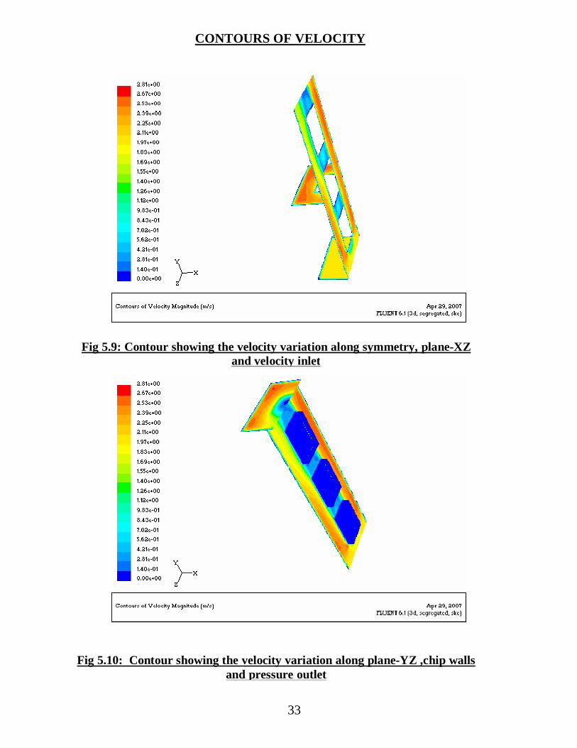
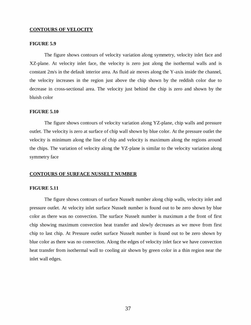
CONTOURS OF VELOCITY
FIGURE 5.9
The figure shows contours of velocity variation along symmetry, velocity inlet face and
XZ-plane. At velocity inlet face, the velocity is zero just along the isothermal walls and is
constant 2m/s in the default interior area. As fluid air moves along the Y-axis inside the channel,
the velocity increases in the region just above the chip shown by the reddish color due to
decrease in cross-sectional area. The velocity just behind the chip is zero and shown by the
bluish color
FIGURE 5.10
The figure shows contours of velocity variation along YZ-plane, chip walls and pressure
outlet. The velocity is zero at surface of chip wall shown by blue color. At the pressure outlet the
velocity is minimum along the line of chip and velocity is maximum along the regions around
the chips. The variation of velocity along the YZ-plane is similar to the velocity variation along
symmetry face
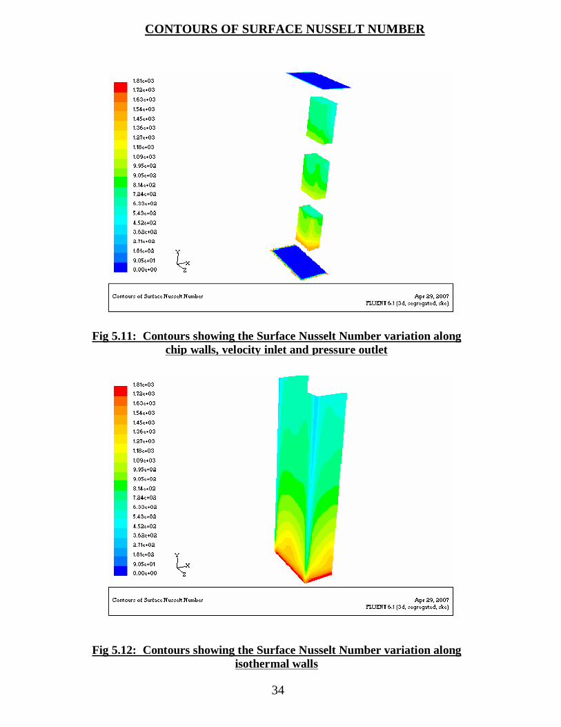
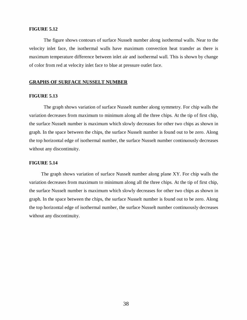
CONTOURS OF SURFACE NUSSELT NUMBER
FIGURE 5.11
The figure shows contours of surface Nusselt number along chip walls, velocity inlet and
pressure outlet. At velocity inlet surface Nusselt number is found out to be zero shown by blue
color as there was no convection. The surface Nusselt number is maximum a the front of first
chip showing maximum convection heat transfer and slowly decreases as we move from first
chip to last chip. At Pressure outlet surface Nusselt number is found out to be zero shown by
blue color as there was no convection. Along the edges of velocity inlet face we have convection
heat transfer from isothermal wall to cooling air shown by green color in a thin region near the
inlet wall edges.
37
45
FIGURE 5.12
The figure shows contours of surface Nusselt number along isothermal walls. Near to the
velocity inlet face, the isothermal walls have maximum convection heat transfer as there is
maximum temperature difference between inlet air and isothermal wall. This is shown by change
of color from red at velocity inlet face to blue at pressure outlet face.
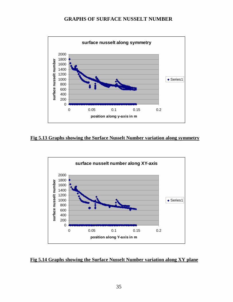
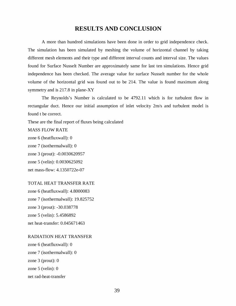
GRAPHS OF SURFACE NUSSELT NUMBER
FIGURE 5.13
The graph shows variation of surface Nusselt number along symmetry. For chip walls the
variation decreases from maximum to minimum along all the three chips. At the tip of first chip,
the surface Nusselt number is maximum which slowly decreases for other two chips as shown in
graph. In the space between the chips, the surface Nusselt number is found out to be zero. Along
the top horizontal edge of isothermal number, the surface Nusselt number continuously decreases
without any discontinuity.
FIGURE 5.14
The graph shows variation of surface Nusselt number along plane XY. For chip walls the
variation decreases from maximum to minimum along all the three chips. At the tip of first chip,
the surface Nusselt number is maximum which slowly decreases for other two chips as shown in
graph. In the space between the chips, the surface Nusselt number is found out to be zero. Along
the top horizontal edge of isothermal number, the surface Nusselt number continuously decreases
without any discontinuity.
38
46
RESULTS AND CONCLUSION
A more than hundred simulations have been done in order to grid independence check.
The simulation has been simulated by meshing the volume of horizontal channel by taking
different mesh elements and their type and different interval counts and interval size. The values
found for Surface Nusselt Number are approximately same for last ten simulations. Hence grid
independence has been checked. The average value for surface Nusselt number for the whole
volume of the horizontal grid was found out to be 214. The value is found maximum along
symmetry and is 217.8 in plane-XY
The Reynolds’s Number is calculated to be 4792.11 which is for turbulent flow in
rectangular duct. Hence our initial assumption of inlet velocity 2m/s and turbulent model is
found t be correct.
These are the final report of fluxes being calculated
MASS FLOW RATE
zone 6 (heatfluxwall): 0
zone 7 (isothermalwall): 0
zone 3 (prout): -0.0030620957
zone 5 (velin): 0.0030625092
net mass-flow: 4.1350722e-07
TOTAL HEAT TRANSFER RATE
zone 6 (heatfluxwall): 4.8000083
zone 7 (isothermalwall): 19.825752
zone 3 (prout): -30.038778
zone 5 (velin): 5.4586892
net heat-transfer: 0.045671463
RADIATION HEAT TRANSFER
zone 6 (heatfluxwall): 0
zone 7 (isothermalwall): 0
zone 3 (prout): 0
zone 5 (velin): 0
net rad-heat-transfer
39
47
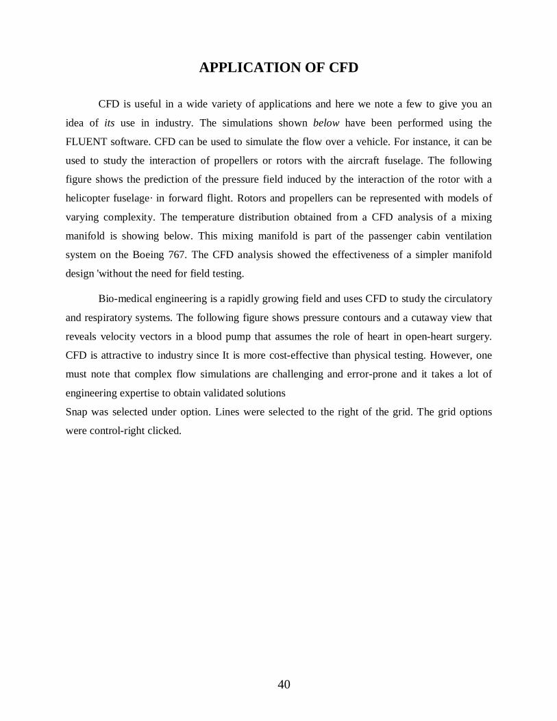
APPLICATION OF CFD
CFD is useful in a wide variety of applications and here we note a few to give you an
idea of its use in industry. The simulations shown below have been performed using the
FLUENT software. CFD can be used to simulate the flow over a vehicle. For instance, it can be
used to study the interaction of propellers or rotors with the aircraft fuselage. The following
figure shows the prediction of the pressure field induced by the interaction of the rotor with a
helicopter fuselage· in forward flight. Rotors and propellers can be represented with models of
varying complexity. The temperature distribution obtained from a CFD analysis of a mixing
manifold is showing below. This mixing manifold is part of the passenger cabin ventilation
system on the Boeing 767. The CFD analysis showed the effectiveness of a simpler manifold
design 'without the need for field testing.
Bio-medical engineering is a rapidly growing field and uses CFD to study the circulatory
and respiratory systems. The following figure shows pressure contours and a cutaway view that
reveals velocity vectors in a blood pump that assumes the role of heart in open-heart surgery.
CFD is attractive to industry since It is more cost-effective than physical testing. However, one
must note that complex flow simulations are challenging and error-prone and it takes a lot of
engineering expertise to obtain validated solutions
Snap was selected under option. Lines were selected to the right of the grid. The grid options
were control-right clicked.
40
48
BIBLIOGRAPHY
[1]. Bergles A.E and Bar Cohen, A, Immersion cooling digital computers, cooling of
electronic systems, ;Kakae, S, Yanu, H, and Hijikata, K, Khaver Academic publishers,
Baston M.A pg-539-621, 1994.
[2]. www.fluent.com/ software/ gambit.
[3]. www.hlrn.de/doc/ fluent
[4]. Incropera FP, convection heat transfer in electronic equipment cooling, Journal of heat
transfer 110 (1988).
[5]. Kennedy KJ, Zebib A, combined free and forced convection between vertical and
parallel plates, some case studies. International journal of Hear and Mass Transfer 26
(1990).
[6]. Danielson RD, tousignant, L, and Bar-Cohen, A saturated pool boiling characteristics of
commercially available per flourinated liquids, proc of ASME/ ISME Thermal
engineering joint conference.
[7]. Chrsler, G.M, chu, r.C. and Simons, RE jet impingement Boiling of a dielectric
coolant in narrow gaps, IEEE trans. CHMT -part A, VOL18(3),pg 527-533,1955
[8]. 8086 Microprocessors by D.V. Hall.
[9]. 8085 Microprocessors by Gaonkar.
[10]. Computational Methods for Fluid Dynamics by J.H.Ferziger& M.Peric (3rd edition)
[11]. Computational fluid Dynamics by John D. Anderson.
[12]. Numerical Heat Transfer and Fluid Flow by Suhas V. Patankar
41