Electronic response of graphene to an ultrashortintense terahertz radiation pulse

Kenichi L IshikawaPhoton Science Center, Graduate School of Engineering, The University ofTokyo, 7-3-1 Hongo, Bunkyo-ku, Tokyo 113-8656, JapanE-mail: ishiken@atto.t.u-tokyo.ac.jp

New Journal of Physics 15 (2013) 055021 (27pp)Received 15 March 2013Published 24 May 2013Online at http://www.njp.org/doi:10.1088/1367-2630/15/5/055021

Abstract. We have recently reported a study (Ishikawa 2010 Phys. Rev. B 82201402) on a nonlinear optical response of graphene to a normally incidentterahertz radiation pulse within the massless Dirac fermion (MDF) picture,where we have derived physically transparent graphene Bloch equations (GBE).Here we extend it to the tight-binding (TB) model and oblique incidence.The derived equations indicate that interband transitions are governed by thetemporal variation of the spinor phase along the electron path in the momentumspace and predominantly take place when the electron passes near the Diracpoint. At normal incidence, the equations for electron dynamics within theTB model can be cast into the same form of GBE as for the MDF model.At oblique incidence, the equations automatically incorporate photon drag andsatisfy the continuity equation for electron density. Single-electron dynamicsstrongly depend on the model and pulse parameters, but the rapid variations areaveraged out after momentum-space integration. Direct current remaining afterthe pulse is generated in graphene irradiated by an intense monocycle terahertzpulse, even if it is linearly polarized and normally incident. The generated currentdepends on the carrier-envelope phase, pulse intensity and Fermi energy in acomplex manner.

Content from this work may be used under the terms of the Creative Commons Attribution 3.0 licence.Any further distribution of this work must maintain attribution to the author(s) and the title of the work, journal

citation and DOI.

New Journal of Physics 15 (2013) 0550211367-2630/13/055021+27$33.00 © IOP Publishing Ltd and Deutsche Physikalische Gesellschaft

2

Contents

1. Introduction 22. Normal incidence 3

2.1. Temporal evolution of the electronic wave function . . . . . . . . . . . . . . . 32.2. Electric current . . . . . . . . . . . . . . . . . . . . . . . . . . . . . . . . . . 6

3. Oblique incidence 63.1. Massless Dirac fermion picture . . . . . . . . . . . . . . . . . . . . . . . . . . 73.2. Tight-binding model . . . . . . . . . . . . . . . . . . . . . . . . . . . . . . . 83.3. Comparison with other approaches . . . . . . . . . . . . . . . . . . . . . . . . 9

4. Linear polarization 104.1. Initial momentum parallel to the field . . . . . . . . . . . . . . . . . . . . . . 104.2. Electron dynamics and current at normal incidence . . . . . . . . . . . . . . . 114.3. Single-electron dynamics at oblique incidence . . . . . . . . . . . . . . . . . . 14

5. Circular path surrounding the Dirac point 176. Direct current generation by a monocycle terahertz radiation pulse 197. Conclusions 24Acknowledgments 24Appendix. Universal conductivity 24References 26

1. Introduction

There has been rising interest in graphene [1, 2] over a broad spectrum of fields because ofits potential application in carbon-based electronics as well as the possibility of mimickingand testing quantum relativistic phenomena [3–6]. While unique properties including finiteconductivity at zero carrier concentration [7] and ac and dc universal conductance [8–10]are predicted and observed, interest in the optical response of graphene is even furtherboosted by the advent of terahertz (THz) radiation technology [11, 12]. Especially, remarkableprogress in the development of intense THz sources has enabled the generation of phase-stable, monocycle to a few cycles, transients with field amplitudes exceeding 100 kV cm�1 andeven 1 MV cm�1 [12–16]. This has opened up a new field of high-field physics in condensedmatter, especially graphene [17, 18]. Along these lines, a theoretical description of nonlinearoptical responses of graphene has become one of the key issues [19–30]. Floquet analysis hasprovided valuable information, e.g. on dressed band structure, gap opening [25, 27, 28] andfrequency-dependence of the nonlinear response [20, 22, 23]. However, this approach, assuminga continuous wave, cannot be directly applied to the case of ultrashort pulse irradiation. As fortime-domain microscopic theories, kinetic approaches [18, 19] based on the Boltzmann equationand second-quantization approaches [29, 30] have been reported.

One distinct aspect of THz-pulse interaction with graphene, compared with the case ofnear-infrared and visible pulses, is that the photon energy is much smaller than that requiredfor vertical transition in most of the momentum space. On the other hand, a THz pulse caninduce a large displacement of electrons in the momentum space: transition from one valley toanother is even possible. We have recently studied [26] nonlinear optical responses of graphene,

New Journal of Physics 15 (2013) 055021 (http://www.njp.org/)

3

starting from the time-dependent Dirac equation (TDDE) and focusing on the electronic motionin the momentum space (intraband dynamics) and the interband transition along its trajectory.We have shown that the TDDE can be cast into a form of generalized optical Bloch equations,referred to as graphene Bloch equations (GBE) hereafter, which describe the interplay betweenintraband and interband dynamics in a physically transparent fashion. The previous study [26]was, however, limited to the massless Dirac fermion (MDF) picture and normal incidence.

In this study, we extend it to the tight-binding (TB) model with nearest-neighborinteractions and oblique incidence. Starting from the time-dependent Schrodinger equation(TDSE), we formulate an exact, fully nonperturbative, nonlinear theory of single-electrondynamics and derive formulas for the induced current, applicable to an arbitrary waveformand polarization of THz pulse, both for normal (section 2) and oblique incidence (section 3). Inthe case of normal incidence, the derived equations can be further cast into the same form ofGBE as within the MDF approximation (section 2). Then, applying them to the case of linearpolarization, we show that interband transitions take place predominantly when the electronpasses near the Dirac point along its trajectory in the momentum space. We examine how theresults depend on the model, pulse parameters and initial electron momentum (section 4). Also,we briefly analyze the single electron dynamics when it takes a circular path around the Diracpoint from the adiabatic limit involving Berry’s phase [31, 32] to the nonadiabatic limit leadingto full population oscillation (section 5). Finally, we study the macroscopic electric currentinduced by an intense monocycle THz pulse and show that the carrier generation through theenhanced interband transition near the Dirac point leads to the generation of a direct current(dc) that remains after the end of the pulse (section 6).

2. Normal incidence

In this section, we treat normal incidence of an optical pulse whose electric field E(t) and vectorpotential A(t) = � R E(t) dt is in the graphene plane (xy plane). The pulse may be of arbitrarytime-dependent polarization, while [26] only considered linear polarization.

2.1. Temporal evolution of the electronic wave function

The TDSE for the two-component wave function (t) of the electron with an initial wave vectorof k (p = hk is the canonical momentum) is given by

ih@

@t (t) = H(t) (t), (1)

where the time-dependent Hamiltonian H(t) is of a form

H(t) =✓

0 h(t)h(t)⇤ 0

◆, h(t) = ✏(t) e�i✓(t), (2)

where ✏(t) = |h(t)| and ✓(t) = � arg h(t).Within the framework of the 2D TB model of nearest-neighbor interactions [5, 33]

h(t) = ��3X

↵=1

ei ·�↵ (3)

with � ⇡ 2.5–2.8 eV being the nearest neighbor hopping energy. �1 = a(0, 1) and �2,3 =a2 (±

p3, �1) are the locations of nearest neighbors separated by distance a ⇡ 1.42 Å. = ⇡/h,

New Journal of Physics 15 (2013) 055021 (http://www.njp.org/)

4

Figure 1. Contour and false color plots of (a) ✏k and (b) the principal value�Arg hk, defined in the range [�⇡,⇡). The thick solid and dashed white squaresin panel (a) outline examples of the simulational Brillouin zone, i.e. the areaof integration in equation (17). The Dirac points K and K 0 are located at(± 2⇡

3p

3, 2⇡

3 ) = (±1.2092, 2.0944). In panel (b), the value jumps between ⇡ and�⇡ on solid white lines.

where ⇡(t) = p + eA(t) is the kinetic momentum with e (> 0) being the elementary charge. ✏ isthe magnitude of the energy eigenvalue for the field-free case; its value ✏k is given by

✏k = �

s

3 + 2 cosp

3kxa + 4 cos

p3kxa2

cos3kya

2, (4)

which we depict in figure 1(a).Sufficiently near the Dirac point, the MDF picture is valid [5]; equation (3) can be

approximated as

h(t) = vF(⇡x � i⇡y), (5)

where vF = 3� a2h ⇡ c/300 and the Dirac point is taken as the origin of ⇡ . Then, we obtain

✏(t) = vF|⇡(t)| = vFh|(t)|, (6)

and ✓ corresponds to the directional angle of satisfying x = | |cos ✓ and y = | |sin ✓(around K), �| |sin ✓ (around K0).

If h(t) is constant independent of time, for both the TB and MDF models, the TDSEequation (1) has the following two solutions:

(t) = 1p2

exp✓

⌥i✏

ht◆✓

e� i2 ✓

± ei2 ✓

◆(7)

whose energy eigenvalues are ±✏, where the upper and lower signs correspond to the upperband (electron band) and the lower band (hole band), respectively.

New Journal of Physics 15 (2013) 055021 (http://www.njp.org/)

5

For the general case of time-dependent h(t), let us make the following ansatz:

(t) = c+(t) +(t) + c�(t) �(t), (8)

i.e. a linear combination of the instantaneous upper and lower band states (Volkov states)

±(t) = 1p2

exp [⌥i�(t)]✓

e� i2 ✓(t)

± ei2 ✓(t)

◆, (9)

where the instantaneous temporal phase or dynamical phase �(t) is defined as

�(t) =Z✏(t)

hdt. (10)

Substituting equations (8) and (9) into equation (1), we obtain, as a temporal variation of theexpansion coefficients c±(t),

c±(t) = i2✓(t)c⌥(t) e±2i�(t). (11)

Introducing the interband coherence ⇢ = c+c⇤� and population difference n = |c+|2 � |c�|2, one

can rewrite equation (11) into the form of GBE [26]:

⇢ = � i2✓(t)n(t) e2i�(t), (12)

n = �i ✓(t)⇢(t) e�2i�(t) + c.c. (13)

We previously derived equations (11)–(13) for the MDF model [26], but they are equallyvalid for the TB model. While equations (11)–(13) basically describe interband transitions,they incorporate field-induced intraband dynamics through �(t) and ✓(t) and are physicallymore transparent than the TDSE. At the same time, they are totally equivalent with theTDSE involving no approximation. The electron dynamics described by the GBEs may beexperimentally probed, e.g. by time-resolved pump–probe photoemission spectroscopy [34].

It should be noted that if ✓(t) were defined by the principal value ✓(t) = �Arg h(t),with Arg z defined in the interval (�⇡,⇡], as plotted in figure 1(b), ✓(t) would undergo 2⇡jumps on the white lines linking the Dirac points in figure 1(b). Here, instead, we are todefine ✓(t) = � arg h(t), with arg z = Arg z + 2⇡n (n is an integer), in such a way that it variescontinuously along the path of (t). Then, if (t) eventually returns to its original position inthe k-space along a trajectory surrounding a Dirac point, ±(t) acquires a geometrical phase of⇡ , in addition to the dynamical phase�(t). Berry’s phase [31, 32] is, hence, incorporated in theGBEs (see section 5).

It is noteworthy that GBEs do not explicitly contain optical matrix elements but thatthe interband transitions are governed by ✓ , which is, especially within the MDF picture, thetemporal variation of the polar angle along the path that (t) takes on the k plane. This indicatesthat an optical-pulse irradiation can be viewed as a means to move an electron along a path inthe k-space. The coupling element ✓(t) is, in the MDF picture, explicitly given by

✓(t) =

8>><

>>:

e[Ex(t)⇡y(t) � Ey(t)⇡x(t)]|⇡(t)|2 (around K),

�e[Ex(t)⇡y(t) � Ey(t)⇡x(t)]|⇡(t)|2 (around K0),

(14)

which is nonlinear in E(t).

New Journal of Physics 15 (2013) 055021 (http://www.njp.org/)

6

2.2. Electric current

The electric current by a single electron is given by �eje, where je is defined as

je = †(t)@H@⇡

(t). (15)

With the solutions ⇢(t) and n(t) of the GBEs (12) and (13), equation (15) can be rewritten as,for the case of the TB model,

je = �

h

3X

↵=1

[n sin ( · �↵ + ✓) � i{⇢ e�i2� cos ( · �↵ + ✓) � c.c.}]�↵, (16)

where the first and second terms correspond to the contribution from the intraband current andinterband polarization, respectively.

To take into account the Fermi distribution, we solve equations (12) and (13) with initialconditions n = F(p) � F(�p) and ⇢ = 0, where F(p) = {1 + exp[(✏(p) � µ)/kBT ]}�1 is theFermi-Dirac function with µ, kB and T being the chemical potential, Boltzmann constantand temperature, respectively. Then, we can obtain the macroscopic electric current J(t) byintegration over the honey-comb lattice Brillouin zone depicted in figure 1(a) as

J(t) = � gse(2⇡)2

Z

BZjc(t) dk, (17)

where gs = 2 denotes the spin-degeneracy factor. The carrier current jc is calculated by replacingn with the carrier occupation n + 1 in equation (16).

In the MDF picture, each component of equation (15) can be explicitly written asje,x = vF

⇥n cos ✓ + i sin ✓{⇢ e�2i� � c.c.}⇤ , (18)

je,y = vF⇥n sin ✓ � i cos ✓{⇢ e�2i� � c.c.}⇤ . (19)

The macroscopic electric current J(t) is given by

J(t) = � gsgve(2⇡ h)2

Zjc(t) dp = � gsgve

(2⇡)2

Zjc(t) dk, (20)

where gv = 2 denotes the valley-degeneracy factor. The carrier current jc is calculated byreplacing n with the carrier occupation n + 1 in equations (18) and (19), i.e.

jc,x = vF⇥(n + 1) cos ✓ + i sin ✓{⇢ e�2i� � c.c.}⇤ , (21)

jc,y = vF⇥(n + 1) sin ✓ � i cos ✓{⇢ e�2i� � c.c.}⇤ . (22)

If we use the MDF model, the whole dynamics is invariant under the multiplication of quantitiesof energy dimension, h!, vF p, vFeA, µ, kBT and h/t , by a common factor. In the weak-field limit, one can derive the universal conductivity e2/4h from equations (20)–(22) (seethe appendix).

3. Oblique incidence

In this section, we extend the formulation developed in the previous section to the case ofoblique incidence. Let us consider an oblique incidence of a pulse whose phase velocity vectorin the xy plane is u = (ux , uy), related to the carrier frequency ! and the wave vector q in thexy plane as q = (!/ux ,!/uy). Note that |u| = c/sin� , with c and � being the vacuum velocityof light and the angle of incidence, respectively. The limit ux , uy ! 1, i.e. q ! 0 correspondsto normal incidence.

New Journal of Physics 15 (2013) 055021 (http://www.njp.org/)

7

slope =�

qy

py

= vF py= �vF py

py

+

�

Figure 2. Schematic representation of the relation between p and ✏± for the caseof p and q parallel to the y-axis.

3.1. Massless Dirac fermion picture

Let us begin with the MDF picture. The TDSE reads

ih@

@t (t, x, y) = vF

� · ⇡

✓t � x

ux� y

uy

◆� (t, x, y). (23)

Through variable transformation (t, x, y) ! (⌧, x, y) with ⌧ ⌘ t � x/ux � y/uy , i.e. in a frameof reference comoving with the pulse, equation (23) can be rewritten as

ih⇣

I � vF

!� · q

⌘ @

@⌧ (⌧, x, y) = vF� · ⇡(⌧ ) (⌧, x, y), (24)

where � and I denote the Pauli and identity matrix, respectively. This equation can also beobtained by replacing ⇡(t) in equation (5) with ⇡(⌧ ) + ih q

!@@⌧

.To obtain insight into equation (24), let us consider the field-free case, i.e. A(⌧ ) = 0 and

⇡(⌧ ) = p. The eigenvalue equation for of temporal and spatial dependence / exp[�i(✏⌧ �p · r)/h] = exp[�i(✏t � (p + ✏

!q) · r)/h], with r = (x, y) is

✏2 � v2F

���p +✏

!q���2= 0, (25)

which can be solved analytically. It should be noticed that replacing p = p + ✏!

q with p wouldlead to the regular eigenvalue equation (6) and that the momentum p in the ⌧ -frame correspondsto p + ✏

!q in the t-frame. These circumstances are schematically depicted in figure 2. Let us

denote the two solutions of equation (25) as ✏+,p(> 0) and ✏�,p(< 0). These two states wouldbe coupled by a photon that has the same in-plane phase velocity u as the incident pulse. Thisobservation indicates that equation (24) automatically incorporates photon drag [35].

New Journal of Physics 15 (2013) 055021 (http://www.njp.org/)

8

We now consider the solution of equation (24) in the presence of an external field A(⌧ ).Again, let us write (⌧ ) as a linear combination of the instantaneous upper and lower bandstates:

(⌧ ) = c+(⌧ ) +(⌧ ) + c�(⌧ ) �(⌧ ) (26)

with

±(⌧ ) = 1p2

exp⇥�i�±(⌧ )

⇤ ✓ e� i2 ✓±(⌧ )

± ei2 ✓±(⌧ )

◆, (27)

where

�±(⌧ ) =Z✏±,⇡(⌧ )

hd⌧, (28)

and ✓±(⌧ ) denote the directional angle of vector ⇡ + ✏±,⇡

!q. Unlike for normal incidence, the

dynamical phase�± and directional angle ✓± are distinct for each band. Then, we obtain, as thetemporal evolution of the expansion coefficients c±,

c±(⌧ ) = i2✓⌥(⌧ ) e±i1�(⌧ )

✓cos

1✓

2

◆�1

c⌥(⌧ ) ± ✓±2

c±(⌧ ) tan1✓

2, (29)

where 1�=�+ ��� and 1✓ = ✓+ � ✓�. In contrast to equation (11), these coupled equationscontain diagonal terms (the second terms) and cannot be cast into a simple form of GBE. Onerecovers equation (11) for the limit of normal incidence, i.e. q ! 0, for which 1✓ ! 0. Itshould be noted that the dynamics described by these equations are not unitary, i.e. a(⌧ ) =|c+(⌧ )|2 + |c�(⌧ )|2 is not constant and a(⌧ ) 6= 1 even after the pulse in general, whose physicalimplication will be discussed below in section 4.3.

The single electron current can be evaluated by

je(⌧ ) = vF †(⌧ )� (⌧ ), (30)

of which each component can be explicitly written as

je,x = vF⇥|c+|2 cos ✓+ � |c�|2 cos ✓� + i sin ✓{⇢ e�i1� � c.c.}⇤ , (31)

je,y = vF⇥|c+|2 sin ✓+ � |c�|2 sin ✓� � i cos ✓{⇢ e�i1� � c.c.}⇤ , (32)

where ✓ = (✓+ + ✓�)/2 and ⇢ = c+c⇤�. Again, the first and second terms correspond to intraband

currents and the third terms to the interband polarization oscillating in time. Let us denote theelectric current for a single electron initially in the upper (lower) band as j+

e (j�e ) and also denotethe current by �(⌧ ) as j0

e(⌧ ). Then, the macroscopic current density can be calculated as

J(⌧ ) = � gsgve(2⇡ h)2

Z ⇥F(✏+,p)j+

e (⌧ ) + F(✏�,p)j�e (⌧ ) � j0e(⌧ )

⇤dp. (33)

3.2. Tight-binding model

Here we follow an approach similar to the one in the previous subsection. The TDSE in the⌧ -frame is

ih@

@⌧ p = H⇡ p, (34)

New Journal of Physics 15 (2013) 055021 (http://www.njp.org/)

9

where ⇡ = p + eA(t � q · r/!) = p + eA(⌧ ). In the ⌧ -frame, h⇡ in H⇡ is given by

h⇡ = ��3X

↵=1

ei⇡ ·�↵/h e�(q·�↵/!)@⌧ . (35)

For the field-free case, this can be rewritten as

hp = ��3X

↵=1

exphi⇣

p +✏

!q⌘

· �↵/hi, (36)

then the energy eigenvalue ✏ satisfies

✏2 = � 2

1 + 4 cos2 a

2h

⇣px +

✏

!qx

⌘

+ 4 cosa

2h

⇣px +

✏

!qx

⌘cos

p3a

2h

⇣py +

✏

!qy

⌘#

. (37)

Hence, as in the case of Dirac fermion, equation (34) incorporates photon drag.Let us rewrite equation (34) as

ih@

@⌧ = H

⇣⇡ + ih

q!@⌧

⌘ , (38)

denote the two solutions of equation (37) as ✏+(> 0) and ✏�(< 0) and make ansatzequations (26) and (27) with ✓± being the phase angle of h⇤

⇡ . Here, h⇡ is given by equation (36)with p replaced by ⇡ . Then, equation (29) holds as coupled differential equations describing thetemporal evolution of the expansion coefficients c±(⌧ ).

The single electron current equation (15) can be evaluated as

je(⌧ ) = �

h

3X

↵=1

⇥|c+|2 sin ( · �↵ + ✓+) � |c�|2 sin ( · �↵ + ✓�)

� i�⇢ e�i1� cos

� · �↵ + ✓

�� c.c. ⇤

�↵, (39)

which tends to equation (16) if q ! 0; the macroscopic current density can be calculated by

J(⌧ ) = � gse(2⇡ h)2

Z

BZ

⇥F(✏+,p)j+

e (⌧ ) + F(✏�,p)j�e (⌧ ) � j0e(⌧ )

⇤dp. (40)

3.3. Comparison with other approaches

It may be worth, at this stage, briefly comparing our approach with some others. Commonapproaches consider a distribution function, say fk, in the k-space and look at its temporalevolution. This view may be said to be analogous in spirit to the Eulerian specification inhydrodynamics, i.e. a way of looking at fluid motion that focuses on specific locations inthe space. References [18, 19, 29, 30] belong to this class. In contrast, our approach, whichmay be called a dynamic first-quantized approach [22], follows the motion of each electron inthe k-space starting from the TDSE, thus, analogous to the Lagrangian specification to followan individual fluid parcel as it moves. While the two views can, in principle, be transformedto each other, our approach helps us to intuitively visualize the large displacement of each

New Journal of Physics 15 (2013) 055021 (http://www.njp.org/)

10

electron (in the k-space) induced by an intense THz radiation field and allows us, for instance,to obtain simple solutions for a circular path around the Dirac point (see section 5). Moreover,whereas [18, 19, 29, 30] apparently assume normal incidence, here we have also presented atreatment of oblique incidence and can account for the effect of photon momentum (see figure 11below), which have been neglected in those studies.

Kao et al [22] and Lopez–Rodrıguez and Naumis [27, 28] took a Lagrangian approachand analyzed the cases of constant electric fields [22] and continuous waves [22, 27, 28].The latter authors also considered oblique incidence. Our approach basically includes these asspecial cases. Moreover, we have derived equations (11) and (29) of motion for the expansioncoefficients c±, which provide us with a clear physical view.

The microscopic approaches in [18, 29, 30] include carrier–carrier and/or carrier–phononscattering processes, which have been neglected in this study. Although further theoreticaldevelopments are required, it is expected that our approach may, in principle, treat these effectsmicroscopically as jumps in the k-space. Alternatively, the mean-field effect may be taken intoaccount through a self-consistent treatment as in [19].

4. Linear polarization

In this section, we examine the electron dynamics and generated current predicted by our theorydeveloped in the previous sections, for the case of linear polarization.

4.1. Initial momentum parallel to the field

Let us begin with the simplest case where the canonical momentum is parallel to the field, i.e.p//A(t), for the case of normal incidence.

In the MDF picture, ✓(t) is nonzero only at the Dirac point where ✓(t) changes stepwise.As can be easily verified, equation (1) has the following two analytical solutions:

(t) = 1p2

exp [�i3(t) dt]✓

e� i2 ✓k

ei2 ✓k

◆,

1p2

exp [i3(t) dt]✓

e� i2 ✓k

�ei2 ✓k

◆(41)

with

3(t) = vF

h

Zn · ⇡(t) dt, (42)

where ✓k denotes the directional angle of k, i.e. the initial value of ✓ and n ⌘ (cos ✓k, sin ✓k).One can also verify that these solutions satisfy equations (8)–(11). It can be easily shown that,for each branch, the current je = vF

†� is given by

je = vF n, and je = �vF n, (43)

respectively. je remains constant, i.e. shows no response for the case of p//A(t). This holdstrue even when the instantaneous kinetic momentum ⇡ = p + eA(t) passes by the Dirac point[⇡(t) = 0]. This situation has been schematically depicted in figure 1 of [26] for ✓k = ⇡ .Remarkably, this result indicates that instantaneous and complete population inversion takesplace at the Dirac point irrespective of the frequency, strength and form of the applied field.

For the case of the TB model, a similar simple analytical solution equation (41) exists onlyfor k = kD + k 0(cos m⇡

3 , sin m⇡3 ) (m = 0, 1, . . . , 5), with kD being the position of a Dirac point.

New Journal of Physics 15 (2013) 055021 (http://www.njp.org/)

11

-1.5

-1.0

-0.5

0.0

(px+eA)/(eA

0)

3.02.52.01.51.00.50.0Time (in optical cycle)

-1.0

-0.5

0.0

0.5

1.0

Pop

ulat

ion

diffe

renc

e n

Figure 3. Temporal evolution of the population difference n(t) between the upperand lower states for px/eA0 = �3/4, h!/vFeA0 = 9.46 ⇥ 10�3 and py/eA0 =0.02 (solid lines) and 0.2 (pink dotted line). The red line is for the MDF model,while the others are for the TB model for the frequency and field strengthindicated in the legend. Also, [px + eA(t)]/eA0 is plotted in a black solid line(right axis).

For example, for k = (k, 0) and an incident light linearly polarized along the x axis, 3(t) isgiven by

3(t) = ��h

Z

1 + 2 cos

p3

2a

!

dt. (44)

4.2. Electron dynamics and current at normal incidence

In order to gain insight into how the electron behaves when ⇡(t) passes near the Dirac point, letus consider a flat-top pulse with a half-cycle ramp-on, normally incident and linearly polarizedalong the x-axis:

Ax(t) =(

A0!t⇡

sin!t (06 t < ⇡/!),

A0 sin!t (⇡/! 6 t),Ay(t) = 0, (45)

where A0 > |px |. We numerically solve the GBEs for an electron initially in the lower bandusing the Bulirsch–Stoer method with adaptive stepsize control [36] for parameters px/eA0 =�3/4, h!/vFeA0 = 9.46 ⇥ 10�3 and different values of py/eA0, where px and py are measuredfrom the Dirac point K = ( 2⇡

3p

3a, 2⇡

3a ) (figure 1). We set � = 2.8 eV in this section. Theseparameters correspond, e.g. to radiation of 0.25 (1, 4) THz frequency with a field strength of2.0 (31.5, 504) kV cm�1.

Figure 3 plots the calculated temporal evolution of the population difference n(t) betweenthe upper (conduction) and lower (valence) states. As we have seen in equation (14), thecoupling element ✓(t) that governs interband transition is nonlinear in E(t) and, when py ismuch smaller than eA0, strongly peaks within a narrow time window around ⇡x(t) = px +A(t) = 0. This leads to a quasi-step-like population transfer (enhanced interband transitions)when ⇡x(t) changes its sign, e.g. when the electron momentum passes near a Dirac point, while

New Journal of Physics 15 (2013) 055021 (http://www.njp.org/)

12

-1.0

-0.5

0.0

0.5

1.0

Pop

ulat

ion

diffe

renc

e n

43210Time (in optical cycle)

(a) 1 THz, 31.5 keV/cm 0 deg 15 30 45 60 75 90 105 MDF

-1.0

-0.5

0.0

0.5

1.0

Pop

ulat

ion

diffe

renc

e n

43210Time (in optical cycle)

(b) 4 THz, 504 keV/cm 0 deg 15 30 45 60 75 90 105 MDF

Figure 4. Temporal evolution of the population difference n(t) between the upperand lower states, calculated within the TB model for different polarization angles⇠ indicated in the legend, for px/eA0 = �3/4, h!/vFeA0 = 9.46 ⇥ 10�3 andpy/eA0 = 0.02. (a) and (b) are for a field strength of 31.5 and 504 keV cm�1,respectively. The result of the MDF model, independent of polarization and fieldstrength, is also plotted by a thick gray line.

n(t) is virtually constant otherwise (see solid lines for py/A0 = 0.02). Especially for py = 0, thepopulation is completely inverted at the Dirac point, as discussed in the previous subsection. Onthe other hand, for py/eA0 & 0.2, there is practically no transition (pink dotted line in figure 3).

We also compare the results of the MDF and TB models in figure 3. For fixed values ofpx/eA0, py/eA0 and h!/vFeA0, the MDF model gives the same result, as we have alreadymentioned. The results of the TB model, on the other hand, depend on the pulse frequency (orfield strength). We can see that all the four solid lines overlap with each other till ⇡ 1.3 cycles(before the second population jump), since the first jump takes place near the Dirac point, wherethe MDF model is a good approximation. After the first jump, the electron is in a superpositionof the upper and lower states. Then, the phase difference accumulated in ⇢ (equation (12))depends on whether one treats the dynamics within the MDF or TB model and further on fieldstrength in the latter, through ✓ and �. Therefore, the population dynamics sensitively dependson the simulation conditions.

Figure 4 illustrates the dependence on pulse polarization up to four optical cycles. Wedenote the polarization direction by the angle ⇠ measured counterclockwise from the x directionand use the initial momentum of the electron rotated by the same angle ⇠ around the Dirac pointK , to make a consistent comparison. Again, although the result is virtually independent ofpolarization before the second interband jump, the dynamics is very sensitive to ⇠ thereafter.One also notices that, at the lower intensity (panel (a)), the MDF is still a relatively goodapproximation before the third jump (. 2.1 cycles), compared with the case of the higherintensity (panel (b)). In figure 5, we show the results for longer times up to sixty cycles.Remarkably, the population dynamics exhibits quasi (but not completely)-periodic behavior.Its period varies with the polarization angle. For example, it is about 22 cycles at ⇠ = 0�, whileabout six cycles at 45�.

New Journal of Physics 15 (2013) 055021 (http://www.njp.org/)

13

-1.0

-0.5

0.0

0.5

1.0

6050403020100

(a) 0 deg

(d) 45 deg

(b) 15 deg (c) 30 deg

(e) 60 deg (f) 75 deg

(i) MDF(g) 90 deg (h) 105 deg

Time (in optical cycle)

Pop

ulat

ion

diffe

renc

e n

-1.0

-0.5

0.0

0.5

1.0

6050403020100-1.0

-0.5

0.0

0.5

1.0

6050403020100-1.0

-0.5

0.0

0.5

1.0

6050403020100

-1.0

-0.5

0.0

0.5

1.0

6050403020100-1.0

-0.5

0.0

0.5

1.0

6050403020100-1.0

-0.5

0.0

0.5

1.0

6050403020100

-1.0

-0.5

0.0

0.5

1.0

6050403020100-1.0

-0.5

0.0

0.5

1.0

6050403020100

Figure 5. (a)–(h) Long-time evolution of the population difference n(t)calculated within the TB model for the polarization angle indicated in each panel.The simulation condition is the same as in figure 4(b). Panel (i) is the result ofthe MDF model.

Let us now look at figure 6, which plots the x component of the macroscopic electric currentinduced by the pulse used in figure 4(b), calculated using the MDF (equation (20)) and TB(equation (17)) models at different polarization angles ⇠ in the latter. The y component vanishesfor the MDF model and the TB model at ⇠ = 0� due to symmetry and virtually vanishes also forthe other values of ⇠ . We see that the current does not linearly follow the ramp-up of the pulseshown in figure 3, indicating a nonlinear nature of the electronic response of graphene, whichwill be discussed further in section 6. The MDF model overestimates the current only slightly;the variation with the polarization direction of the pulse within the TB model is negligibly small.This observation may come as a surprise, especially after having seen the sensitive dependencein figures 4 and 5, but can be understood as follows. The sensitiveness of the single-electronresponse to the model and pulse conditions is due to that of the phase of ⇢ (equation (12))accumulated through ✓ and � along the electron path in the momentum space. The latter isexpectedly affected also by the initial momentum p. Indeed, in figure 7, which illustrates thedependence of the x component of single-electron fluence

R | jc,x(t)|2 dt integrated up to sixcycles on initial momentum, we see that the contribution to the current rapidly changes withthe initial momentum and forms a complicated interference pattern, which also depends onwhether we calculate using the MDF or TB model. Integrated over the momentum space, suchfine interference as well as the sensitive dependence in figures 4 and 5 are mostly averaged out,resulting in the weak dependence seen in figure 6.

New Journal of Physics 15 (2013) 055021 (http://www.njp.org/)

14

-4x10-4

-2

0

2

4

Mac

rosc

opic

ele

ctric

cur

rent

(a.u

.)

6543210Time (in optical cycle)

MDF TB 0 deg 15 deg 30 deg

4 THz, 504 keV/cm

Figure 6. Temporal variation of the x component of the macroscopic electriccurrent equation (20) within the MDF picture (black) and equation (17) withinthe TB model at polarization angle ⇠ = 0� (red), 15� (blue) and 30� (green), forthe case of figure 4(b). The Fermi energy and temperature are assumed to beµ = 0 and T = 0, respectively.

4.3. Single-electron dynamics at oblique incidence

We have examined normal incidence so far. Let us now turn to oblique incidence. Here, weconsider a pulse propagating in the y direction (ux = 0 and uy = c/sin� ) and polarized in the xdirection whose vector potential is given by

Ax(⌧ ) = A0(⌧ ) sin(!⌧ ), Ay(⌧ ) = 0, (46)

where A0(⌧ ) denotes the envelope function. Specifically, we assume a central frequency of10 THz, a peak intensity of 107 W cm�2 corresponding to a 87 kV cm�1 field strength and aGaussian temporal profile with a full-width at half-maximum (FWHM) of 300 fs. Figure 8plots the population dynamics, calculated within the MDF model, of an electron initially inthe valence band with an initial t-frame momentum p = p + ✏

!q of px = 0 and py = Amax/5,

where Amax denotes the peak vector potential. We compare the results for � = ⇡4 and 0. Both,

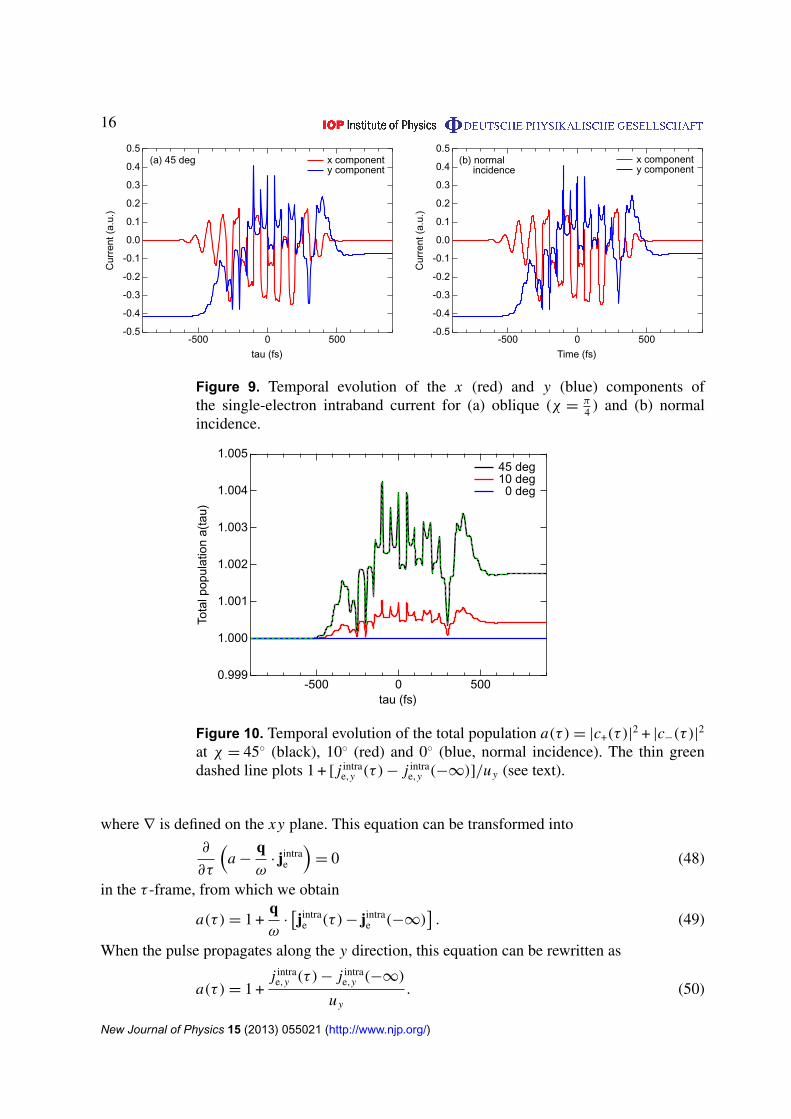
composed of enhanced interband transitions near the Dirac point, are virtually indistinguishablefrom each other. In figure 9 we show the single-electron intraband current jintra

e , i.e. the firstand second terms of equations (31) and (32). Again, the result for oblique incidence (panel(a)) is indistinguishable from that for normal incidence (panel (b)) on the scale of the figures.These observations are due to the fact that the carrier velocity vF is so much smaller thanthe propagation velocity c/sin� of the pulse that the field seen by the electron is practicallyunchanged by the spatial displacement.

A closer look into the total population a(⌧ ), however, reveals a fine but importantdifference, as can be seen in figure 10. It remains at unity for the case of normal incidence,since equation (11) describes a unitary temporal evolution. As we have mentioned in section 3,on the other hand, a(⌧ ) is not constant at oblique incidence and does not return to unity even

New Journal of Physics 15 (2013) 055021 (http://www.njp.org/)

15

2.16

2.14

2.12

2.10

2.08

2.06

2.04

k y a

1.61.41.21.00.8kx a

1.0

0.8

0.6

0.4

0.2

0.0

2.16

2.14

2.12

2.10

2.08

2.06

2.04

k y a

1.61.41.21.00.8kx a

1.0

0.8

0.6

0.4

0.2

0.0

(a)

(b)

Figure 7. The dependence of the x component of the single-electron fluenceR | jc,x(t)|2 dt integrated up to six cycles, on the initial value of ka around theDirac point K , in false-color representation (relative value). (a) TB model with⇠ = 0� and (b) MDF model. K is located at ( 2⇡

3p

3, 2⇡

3 ) = (1.2092, 2.0944).

1.0

0.8

0.6

0.4

0.2

0.0

Pop

ulat

ion

-500 0 500tau (fs)

conduction band valence band total

(a) 45 deg1.0

0.8

0.6

0.4

0.2

0.0

Pop

ulat

ion

-500 0 500Time (fs)

conduction band valence band total

(b) normal incidence

Figure 8. Temporal evolution of the conduction-state (red), valence-state (blue)and total (black) population for (a) oblique (� = ⇡

4 ) and (b) normal incidence.

after the pulse has ended. The variation of a(⌧ ) is physically related to electron balance throughthe continuity equation in the t-frame

@a@t

+ r · jintrae = 0, (47)

New Journal of Physics 15 (2013) 055021 (http://www.njp.org/)

16

-0.5

-0.4

-0.3

-0.2

-0.1

0.0

0.1

0.2

0.3

0.4

0.5

Cur

rent

(a.u

.)

5000-500tau (fs)

x component y component

(a) 45 deg

-0.5

-0.4

-0.3

-0.2

-0.1

0.0

0.1

0.2

0.3

0.4

0.5

Cur

rent

(a.u

.)

5000-500Time (fs)

x component y component

(b) normal incidence

Figure 9. Temporal evolution of the x (red) and y (blue) components ofthe single-electron intraband current for (a) oblique (� = ⇡

4 ) and (b) normalincidence.

1.005

1.004

1.003

1.002

1.001

1.000

0.999

Tota

l pop

ulat

ion

a(ta

u)

5000-500tau (fs)

45 deg 10 deg 0 deg

Figure 10. Temporal evolution of the total population a(⌧ ) = |c+(⌧ )|2 + |c�(⌧ )|2at � = 45� (black), 10� (red) and 0� (blue, normal incidence). The thin greendashed line plots 1 + [ j intra

e,y (⌧ ) � j intrae,y (�1)]/uy (see text).

where r is defined on the xy plane. This equation can be transformed into@

@⌧

⇣a � q

!· jintra

e

⌘= 0 (48)

in the ⌧ -frame, from which we obtain

a(⌧ ) = 1 +q!

· ⇥jintrae (⌧ ) � jintra

e (�1)⇤. (49)

When the pulse propagates along the y direction, this equation can be rewritten as

a(⌧ ) = 1 +j intrae,y (⌧ ) � j intra

e,y (�1)

uy. (50)

New Journal of Physics 15 (2013) 055021 (http://www.njp.org/)

17

1.5x10-2

1.0

0.5

0.0

-0.5

-1.0

Cur

rent

(a.u

.)

5000-500tau (fs)

y component 45 deg 10 deg 0 deg

Figure 11. Temporal evolution of the sum of j intrae,y for p = (0, Amax/5) and

(0, �Amax/5) at � = 45� (black), 10� (red) and 0� (blue, normal incidence).

Equation (50) is plotted in figure 10 by a thin green dashed line for � = 45�, which perfectlyoverlaps with the black line.

Another effect can be found if one looks at the sum of j intrae,y for p = (0, Amax/5) and

(0, �Amax/5), which is plotted in figure 11. While the sum vanishes due to symmetry at normalincidence, it is finite at oblique incidence due to the net momentum exchange with the pulseupon interband transition (figure 2). We also notice that both the deviation of the total populationfrom unity in figure 10 and the sum of j intra

e,y in figure 11 are nearly exactly proportional to sin� .

5. Circular path surrounding the Dirac point

In this short section, let us examine an important, analytically solvable problem, namely, howthe electron behaves when its kinetic momentum vector ⇡(t) varies along a path circulatingaround the Dirac point in such a way that

✓(t) = !t and ✏(t) = const. (51)

Within the MDF picture, the electron takes a circular path around the Dirac point and such asituation may typically be realized under a normal incidence of a circularly polarized pulse. Inthis case, equation (11) can be transformed into a form of the Rabi oscillation

c±(t) = i2! exp(±i⌘!t) c⌥(t), (52)

where ⌘ ⌘ 2✏/h!, which can be analytically solved. For an initial condition c+(0) = 1 andc�(0) = 0, we obtain

c+(t) = expi⌘✓2

0

@cos✓p

1 + ⌘2

2� i⌘ sin ✓

p1+⌘2

2p1 + ⌘2

1

A , (53)

New Journal of Physics 15 (2013) 055021 (http://www.njp.org/)

18

1.0

0.8

0.6

0.4

0.2

0.0

Pop

ulat

ion

of th

e co

nduc

tion

stat

e

2.01.51.00.50.0theta (pi radian)

eta =

2 1 0.5 0.1 0

Figure 12. Conduction-band population when the electron takes a circular patharound the Dirac point.

c�(t) = i exp✓

� i⌘✓2

◆sin ✓

p1+⌘2

2p1 + ⌘2

(54)

and then

|c�(t)|2 = 1 � |c+(t)|2 = sin2 ✓p

1+⌘2

2

1 + ⌘2. (55)

In terms of an analogy to Rabi oscillations, ⌘ plays the role of detuning.Figure 12 shows the population |c+(✓)|2 of the conduction band.In the adiabatic limit ⌘! 1 (or !! 0), the solutions are approximated as c+(t) ⇡ 1 and

c�(t) ⇡ 0. The electron remains in the upper band and when it returns to the original position,i.e. ✓(t) = 2⇡ , its wave function (t) acquires Berry’s phase ⇡ , as theoretically predicted [31]and experimentally confirmed [32].

In the opposite limit ⌘! 0, corresponding to a quick rotation near the Dirac point, thesolutions read as

c+(t) = cos✓(t)

2, and c�(t) = i sin

✓(t)2

. (56)

The electron population is completely transferred to the lower band at ✓(t) = ⇡ . Moreover,whether the electron arrives at the other side of the Dirac point by a counter-clockwise [✓(t) =⇡ ] or clockwise [✓(t) = �⇡ ] half rotation, it ends up with the same wave function, in contrastto the adiabatic limit. These observations are consistent with our discussion in subsection 4.1.After a complete rotation [✓(t) = 2⇡ ], the electron population is transferred back to the upperband, but, since c+ = �1 instead of unity, Berry’s phase is cancelled by a phase acquired throughthe interband dynamics, again in contrast to the adiabatic limit.

It should be noticed that equation (56) also holds for any path of ⇡(t) sufficiently close tothe Dirac point. Indeed, if we approximate�(t) as vanishing, it is easy to see that the following

New Journal of Physics 15 (2013) 055021 (http://www.njp.org/)

19

solutions:

c+(t) = cos✓(t) � ✓(0)

2and c�(t) = i sin

✓(t) � ✓(0)

2(57)

satisfy equation (11).The results in figure 12 can be used to roughly estimate the vertical width of the distribution

presented in figure 7. The population transfer is significant, say, for ⌘ . 1. Using the definitionof ⌘ ⌘ 2✏/h!, the first part of equations (51), (6) and (14) with Ey = 0, Ay = 0 and ⇡x = 0, onecan transform this into

|py|.s

ehE0

2vF, (58)

where py is here measured from the Dirac point and E0 denotes the field amplitude. Thiscriterion corresponds to a full-width of ⇠0.06 for the case of figure 7, which is indeed found tobe a reasonable estimate.

6. Direct current generation by a monocycle terahertz radiation pulse

In this section we investigate the response of graphene to an ultrashort (typically monocycle)intense THz pulse and predict that a direct current is generated that remains after the pulse, evenwhen the pulse is linearly polarized and normally incident.

Let us consider a pulse whose vector potential is given by

A(t) = A0(t) sin(!t +�CE), (59)

where A0(t) and �CE denote the envelope function and the carrier-envelope phase (CEP),respectively. Figure 13(a) shows the temporal evolution of the current Jx(t) for the case ofa monocycle Gaussian 10 THz, 100 fs pulse with a field amplitude E0 of 316 kV cm�1 and�CE = ⇡

2 whose vector potential is shown in figure 13(b). We set T = 0, µ = 0 and vF = c/300(� = 3.09 eV) in this section, unless otherwise stated. Since the MDF and TB models givevirtually the same results (see figure 16(a) below), the former model has been used forfigures 13–15. In the beginning of the pulse, the generated current basically follows the changeof the vector potential with some nonlinearity. On the other hand, in the latter part of the pulse(t & 0), the curve for the current is largely distorted, compared with the vector potential and thecurrent remains finite and virtually constant after the pulse. This indicates that direct current canbe generated in the bulk part of graphene by monocycle terahertz pulses. The contributions fromthe intraband current and interband polarization are also plotted in figure 13(a). One can seethat the dc component is almost entirely due to the former, which implies that carriers remainafter the pulse, asymmetrically distributed in momentum space. Since the interband polarizationgives only a very small fluctuation, we plot only the intraband current in figures 14 and 15 below.

In order to clarify the mechanism of the carrier generation, let us examine how thevariation of Fermi energy µ and pulse intensity affect dc generation. Figure 14(a) presents theCEP dependence of the generated current that remains after the pulse with a field amplitudeof 316 kV cm�1 and for two different values of µ = 0 and 0.3 eV. Since the photon energy(0.041 eV) is much smaller than 0.3 eV, the interband transition through a single- or few-photonsabsorption is suppressed for the case of µ = 0.3 eV. Nevertheless, basically a similar amount ofcurrent is generated for the two cases, though the generated current oscillates with CEP more

New Journal of Physics 15 (2013) 055021 (http://www.njp.org/)

20

-6x10-5

-4

-2

0

2

4

6

Cur

rent

(a.u

.)

6004002000-200Time (fs)

10 THz, 316 kV/cm, 100 fs Total Intraband Interband

(a)

-4x10-2

-2

0

2

4

Vect

or p

oten

tial (

a.u.

)

3002001000-100-200-300Time (fs)

CEP = 0 deg CEP = 90 deg

(b)

Figure 13. (a) Temporal evolution of the current Jx(t) for the case of amonocycle 10 THz, 100 fs pulse with a field amplitude of 316 kV cm�1 whosevector potential is given by equation (59) with �CE = ⇡

2 . (b) Temporal profile ofthe vector potential for �CE = 0 and ⇡

2 .

-1.0x10-5

-0.5

0.0

0.5

1.0

Cur

rent

(a.u

.)

350300250200150100500Carrier-envelope phase (degrees)

10 THz, 100 fs 316 kV/cm, mu = 0 eV 316 kV/cm, mu = 0.3 eV

10 THz, 300 fs 316 kV/cm, mu = 0 eV

(a)

-1.0x10-5

-0.5

0.0

0.5

1.0

Cur

rent

(a.u

.)

350300250200150100500Carrier-envelope phase (degrees)

10 THz, 100 fs 100 kV/cm, mu = 0 eV 100 kV/cm, mu = 0.3 eV

(b)

Figure 14. CEP dependence of the generated intraband current for µ = 0 (red)and 0.3 eV (black), for the case of 100 fs pulse width (monocycle pulse). (a) Fora field amplitude of 316 kV cm�1 and (b) for 100 kV cm�1. In panel (a), the resultfor 300 fs pulse width (three-cycle pulse) and µ = 0 is also plotted (blue).

largely for µ = 0 eV than for 0.3 eV. Therefore, the carrier generation is not due to the single-or few-photons jumping between the bands.

Another possible mechanism of carrier generation is the enhanced interband transition nearthe Dirac point. For this to take place, the displacement |eA(t)| in the momentum space must begreater than the momentum pµ ⌘ |µ/vF| corresponding to the Fermi energy. In figure 14(b) weshow a comparison for the case of a field amplitude of 100 kV cm�1. One finds that dc generationis almost completely suppressed for µ = 0.3 eV. It should be noticed that pµ = 2.41 ⇥ 10�2 a.u.for µ = 0.3 eV is smaller than eA0 = 4.04 ⇥ 10�2 a.u. for E0 = 316 kV cm�1 but larger than1.28 ⇥ 10�2 a.u. for 100 kV cm�1. Thus, we can identify the enhanced interband transition

New Journal of Physics 15 (2013) 055021 (http://www.njp.org/)

21

-1.0x10-5

-0.5

0.0

0.5

1.0

Cur

rent

(a.u

.)

350300250200150100500Carrier-envelope phase (degrees)

10 THz, 100 fs, mu = 0 eV 316 kV/cm 200 100 31.6

(a) 6x10-6

4

2

0

-2

Spe

ctra

l am

plitu

de

2520151050

Spectral order

10 THz, 100 fs, mu = 0 eV 316 kV/cm 200 100 31.6

(b)

Figure 15. (a) CEP dependence of the generated intraband current for differentvalues of field amplitude and (b) spectrum of the CEP dependence (see text).

as the origin of the carrier generation leading to the dc current. Indeed, the direction of theremaining current can be understood as follows. Carrier electrons in the conduction band aremost efficiently generated when the displacement in the momentum space reaches its maximum,i.e. around t = 0. Some of the valence electrons originally with negative px are lifted to theconduction band in the positive px region at this time and then brought back to the negativepx region still in the conduction band, which leads to a positive remaining current, as can beconfirmed in figure 13(a).

In figure 14(a) we also plot the result for a three-cycle pulse (blue line). One can see thatthe remaining current is substantially reduced compared with the case of a monocycle pulse.Hence, the dc generation is a feature unique to ultrashort pulses in the monocycle regime.

Let us now look closely at CEP dependence. In figure 14 we have already seen that thedependence of the dc current J dc remaining after the end of the pulse on �CE is mainly composedof a large, slow oscillation with a period of 2⇡ , superposed by a faster oscillation. Figure 15(a)shows how this oscillation varies with pulse intensity. Interestingly, the more intense the pulse,the higher the modulation frequency. As a consequence, remarkably, the value of J dc at a fixedcarrier envelope phase is a complicated function of intensity (or equivalently, field amplitude).The dependence is clearly nonlinear, but not of simple integer orders. At �CE = 45�, for example,J dc jumps from 1.3 ⇥ 10�6 to 1.2 ⇥ 10�5 when the peak field amplitude increases from 100 to200 kV cm�1, while it is nearly unchanged even when the field amplitude further increases to316 kV cm�1. Moreover, at �CE = 10�, for example, J dc does not vary monotonically with theintensity, even changing its sign.

It follows from the space inversion symmetry and the symmetry between c+ and c� inequation (11) that the generated direct current J dc

1 and J dc2 for the vector potential A1(t) and

A2(t), respectively, satisfies

J dc1 = �J dc

2 if A2(t) = �A1(t). (60)

J dc1 = J dc

2 if A2(t) = A1(�t). (61)

New Journal of Physics 15 (2013) 055021 (http://www.njp.org/)

22

-4x10-5

-2

0

2

4

Mac

rosc

opic

ele

ctric

cur

rent

(a.u

.)

-300 -200 -100 0 100 200 300Time (fs)

TB MDF

(a) 10 THz, 316 kV/cm

-3x10-4

-2

-1

0

1

2

3

Mac

rosc

opic

ele

ctric

cur

rent

(a.u

.)

-300 -200 -100 0 100 200 300Time (fs)

TB MDF

(b) 10 THz, 1 MV/cm

-2x10-3

-1

0

1

2

Mac

rosc

opic

ele

ctric

cur

rent

(a.u

.)

-300 -200 -100 0 100 200 300Time (fs)

TB MDF

(c) 10 THz, 3.16 MV/cm

-1.0x10-2

-0.5

0.0

0.5

1.0

Mac

rosc

opic

el

ectri

c cu

rren

t (a.

u.)

-300 -200 -100 0 100 200 300Time (fs)

TB 0 deg TB 90 deg MDF

(d) 10 THz, 10 MV/cm

Figure 16. Temporal evolution of the current Jx(t), including both the intra-and interband contributions, for the case of a monocycle 10 THz, 100 fsGaussian pulse with a field amplitude of (a) 316 kV cm�1, (b) 1 MV cm�1, (c)3.16 MV cm�1 and (d) 10 MV cm�1, with �CE = ⇡

2 . The red and blue lines arethe results calculated with the MDF model and the TB model with ⇠ = 0�,respectively. In panel (d), the result for ⇠ = 90� is also plotted by a green line.

For the vector potential given by equation (59) with a Gaussian envelope A0(t), theseproperties translate into

J dc(�CE) = �J dc(�CE +⇡) and J dc(�CE) = J dc(⇡ ��CE), (62)

which can be confirmed in figures 14 and 15(a). As a consequence, the CEP dependenceJ dc(�CE) can be expanded in a Fourier sine series as

J dc(�CE) =1X

n=0

f2n+1 sin[(2n + 1)�CE], (63)

where the spectral amplitudes f2n+1 are real. We show the spectrum ( f2n+1 as a function ofspectral order 2n + 1) in figure 15(b). The spectrum is mainly composed of the fundamentalcomponent (first order) and the modulation component (approximately 3rd, 7th and 11th/13thorders, at 100, 200 and 316 kV cm�1, respectively) that shifts to higher orders with an increasein intensity. The behavior in figure 15(b) emphasizes the complex nature of the intensity andCEP dependence of dc generation.

J dc(�CE) vanishes at �CE = 0 and ⇡ . In these cases, as plotted in figure 13(b), the temporalprofile of the vector potential A(t) is symmetric to the positive and negative directions. Thisindicates that one of the origins of the dc generation is a positive-negative asymmetry of thevector potential, i.e. that of the displacement of electrons in the momentum space. Indeed, theasymmetry is largest at �CE = ⇡

2 and 32⇡ , for which |J dc(�CE)| reaches maximum. It should

be, however, emphasized that the interband transition enhanced in the vicinity of the Dirac

New Journal of Physics 15 (2013) 055021 (http://www.njp.org/)

23

2.3

2.2

2.1

2.0

1.9k y

a

3210-1-2-3kx a

1.0

0.8

0.6

0.4

0.2

0.0

(d)

2.3

2.2

2.1

2.0

1.9

k y a

3210-1-2-3kx a

1.0

0.8

0.6

0.4

0.2

0.0

(b)2.3

2.2

2.1

2.0

1.9

k y a

3210-1-2-3kx a

1.0

0.8

0.6

0.4

0.2

0.0

(a)

2.3

2.2

2.1

2.0

1.9

k y a

3210-1-2-3kx a

1.0

0.8

0.6

0.4

0.2

0.0

(c)

Figure 17. The dependence of the x component of the single-electron fluenceR1�1 | jc,x(t)|2 dt on the initial value of ka, calculated with the TB model

at ⇠ = 0�, in false-color representation (relative value). The pulse shape ismonocycle 10 THz, 100 fs Gaussian with a field amplitude of (a) 316 kV cm�1,(b) 1 MV cm�1, (c) 3.16 MV cm�1 and (d) 10 MV cm�1. The Dirac points arelocated at

⇣± 2⇡

3p

3, 2⇡

3

⌘= (±1.2092, 2.0944).

points is another essential factor, since, if this is suppressed by a large Fermi energy, there is noappreciable remaining current, as we have seen in figure 14(b).

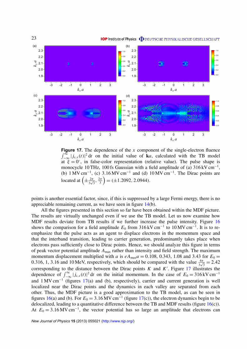
All the figures presented in this section so far have been obtained within the MDF picture.The results are virtually unchanged even if we use the TB model. Let us now examine howMDF results deviate from TB results if we further increase the pulse intensity. Figure 16shows the comparison for a field amplitude E0 from 316 kV cm�1 to 10 MV cm�1. It is to re-emphasize that the pulse acts as an agent to displace electrons in the momentum space andthat the interband transition, leading to carrier generation, predominantly takes place whenelectrons pass sufficiently close to Dirac points. Hence, we should analyze this figure in termsof peak vector potential amplitude Amax rather than intensity and field strength. The maximummomentum displacement multiplied with a is eAmaxa = 0.108, 0.343, 1.08 and 3.43 for E0 =0.316, 1, 3.16 and 10 MeV, respectively, which should be compared with the value 4⇡

3p

3= 2.42

corresponding to the distance between the Dirac points K and K 0. Figure 17 illustrates thedependence of

R1�1 | jc,x(t)|2 dt on the initial momentum. In the case of E0 = 316 kV cm�1

and 1 MV cm�1 (figures 17(a) and (b), respectively), carrier and current generation is welllocalized near the Dirac points and the dynamics in each valley are separated from eachother. Thus, the MDF picture is a good approximation to the TB model, as can be seen infigures 16(a) and (b). For E0 = 3.16 MV cm�1 (figure 17(c)), the electron dynamics begin to bedelocalized, leading to a quantitative difference between the TB and MDF results (figure 16(c)).At E0 = 3.16 MV cm�1, the vector potential has so large an amplitude that electrons can

New Journal of Physics 15 (2013) 055021 (http://www.njp.org/)

24

move between the two Dirac cones (figure 17(d)). The MDF model fails to describe such asituation, leading to even a qualitative discrepancy between the two models, as is clearly seen infigure 16(d). We can also see that dc generation is reduced. Surprisingly, however, even in thiscase, the current depends on pulse polarization ⇠ only moderately (figure 16(d)). The verticalwidth of each distribution in figure 17 can reasonably be predicted by the criterion equation (58)as ⇠0.044, 0.078, 0.14 and 0.25, respectively.

7. Conclusions

Based on both the MDF and the TB models, we have derived equations that describe thecoherent population dynamics of electrons in graphene irradiated by a terahertz radiation pulseof arbitrary wave form, angle of incidence and polarization. These equations are equivalent tothe time-dependent Schrodinger equation and, at the same time, provide a physically transparentdescription of intraband dynamics and interband transitions and polarization. For the case ofnormal incidence, these can be further cast into the form of GBE (12) and (13). We have alsoderived the formula for a single-electron current, the integration of which over the momentumspace leads to a macroscopic current.

The calculations using the derived equations have revealed a sensitive dependenceof the single-electron dynamics on the model, pulse polarization with respect to the latticeand the electron’s initial momentum. This dependence is, however, mostly averaged out afterthe momentum-space integration and thus the macroscopic current exhibits only moderatedependence.

With the help of our formulation, we have obtained exact analytical solutions for thedynamics of a single electron whose kinetic momentum takes a circular path around the Diracpoint. The solutions account for Berry’s phase in the adiabatic limit and predict full populationoscillation in the limit of rapid circulation.

Furthermore, we have shown that a direct current is generated when graphene is subject toa monocycle intense THz pulse, due to enhanced carrier generation taking place when electronspass near the Dirac points.

Acknowledgments

This work was supported by the Advanced Photon Science Alliance (APSA) projectcommissioned by the Ministry of Education, Culture, Sports, Science and Technology (MEXT)of Japan as well as by KAKENHI (no. 23104708).

Appendix. Universal conductivity

In this appendix, we outline the derivation of the universal conductivity [8–10] �0 = e2/4hstarting from the GBEs within the MDF picture. Let us consider normal incidence of asufficiently weak pulse, assumed to be linearly polarized along the x axis without lossof generality. For Ex(t) = E0 cos!t and Ax(t) = �(E0/!) sin!t with E0 being the fieldamplitude, we obtain

✓(t) ⇡ eE0 cos!t sin�p

, (A.1)

New Journal of Physics 15 (2013) 055021 (http://www.njp.org/)

25

from equation (14), where � denotes the initial value of ✓(t) satisfying px = p cos� andpy = p sin� and also

�(t) ⇡ !0t, (A.2)

with !0 = vF p/h. By substituting equations (A.1) and (A.2) to equations (12) and (13), weobtain

⇢ ⇡ �ieE(t) sin�

2pn(t) e2i!0t , (A.3)

n ⇡ �ieE(t) sin�

p⇢(t) e�2i!0t + c.c. (A.4)

By noting the initial condition ⇢(�1) = 0 and n(�1) = �1, assuming zero temperature(T = 0), one obtains n(t) ⇡ 1 and

⇢(t) ⇡ ieE0 sin�

2pe2i!0t(! sin!t + 2i!0 cos!t)

!2 � (2!0)2. (A.5)

By noting

cos ✓(t) ⇡ cos� +eAx(t) sin2 �

p, (A.6)

we obtain, using equation (21),

jx(t) ⇡ vFeAx(t) sin2 �

p!2

!2 � (2!0)2. (A.7)

Now that we have a linear relation between jx and Ax , it is convenient to redefine Ex(t)and Ax(t) as

Ex(t) = E0 ei!t , Ax(t) = i!

E0 ei!t = i!

Ex(t). (A.8)

Then, equation (A.7) is rewritten as

jx(t) ⇡ ivFeEx(t) sin2 �

!p!2

!2 � (2!0)2. (A.9)

Let us now integrate this with respect to p, assuming intrinsic graphene (µ = 0). The totalintegrated current equation (20) is determined by the pole at ! = 2!0, i.e. resonant interbandtransition, leading to

Jx(t) = e2

4hEx(t), (A.10)

which indicates the universal conductivity.

New Journal of Physics 15 (2013) 055021 (http://www.njp.org/)

26

References

[1] Novoselov K S, Geim A K, Morozov S V, Jiang D, Zhang Y, Dubonos S V, Grigorieva I V and Firsov A A2004 Electric field effect in atomically thin carbon films Science 306 666

[2] Berger C et al 2004 Ultrathin epitaxial graphite: 2D electron gas properties and a route toward graphene-basednanoelectronics J. Phys. Chem. B 108 19912

[3] Geim A K and Novoselov K S 2007 The rise of graphene Nature Mater. 6 183[4] Geim A K 2009 Graphene: status and prospects Science 324 1530[5] Castro Neto A H, Guinea F, Peres N M R, Novoselov K S and Geim A K 2009 The electric properties of

graphene Rev. Mod. Phys. 81 109[6] Britnell L et al 2012 Field-effect tunneling transistor based on vertical graphene heterostructures Science

335 947[7] Novoselov K S, Geim A K, Morozov S V, Jiang D, Katsnelson M I, Grigorieva Dubonos S V and Firsov A A

2005 Two-dimensional gas of massless Dirac fermions in graphene Nature 438 197[8] Gusynin V P, Sharapov S G and Carbotte J P 2006 Unusual microwave response of Dirac quasiparticles in

graphene Phys. Rev. Lett. 96 256802[9] Kuzmenko A B, van Heumen E, Carbone F and van der Marel D 2008 Universal optical conductance of

graphene Phys. Rev. Lett. 100 117401[10] Nair R R, Blake P, Grigorenko A N, Novoselov K S, Booth T J, Stauber T, Peres N M R and Geim A K 2008

Fine structure constant defines visual transparency of graphene Science 320 1308[11] Ferguson B and Zhang X-C 2002 Materials for terahertz science and technology Nature Mater. 1 26[12] Hoffmann M C and Fulop J A 2011 Intense ultrashort terahertz pulses: generation and applications J. Phys.

D: Appl. Phys. 44 083001[13] Yeh K-L, Hoffmann M C, Hebling J, Keith A and Nelson K A 2007 Generation of 10 µJ ultrashort terahertz

pulses by optical rectification Appl. Phys. Lett. 90 171121[14] Reimann K, Smith R P, Weiner A M, Elsaesser T and Woerner M 2003 Direct field-resolved detection of

terahertz transients with amplitudes of megavolts per centimeter Opt. Lett. 28 471[15] Hebling J, Yeh K-L, Hoffmann M C, Bartal B and Nelson K A 2008 Generation of high-power terahertz

pulses by tilted-pulse-front excitation and their application possibilities J. Opt. Soc. Am. B 25 B6[16] Hirori H, Doi A, Blanchard F and Tanaka K 2011 Single-cycle terahertz pulses with amplitudes exceeding 1

MV/cm generated by optical rectification in LiNbO3 Appl. Phys. Lett. 98 091106[17] Winnerl S et al 2011 Carrier relaxation in epitaxial graphene photoexcited near the Dirac point Phys. Rev.

Lett. 107 237401[18] Tani S, Blanchard F and Tanaka K 2012 Ultrafast carrier dynamics in graphene under a high electric field

Phys. Rev. Lett. 109 166603[19] Mikhailov S A and Ziegler K 2008 Nonlinear electromagnetic response of graphene: frequency multiplication

and the self-consistent-field effects J. Phys.: Condens. Matter 20 384204[20] Wright A R, Xu X G, Cao J C and Zhang C 2009 Strong nonlinear optical response of graphene in the

terahertz regime Appl. Phys. Lett. 95 072101[21] Mishchenko E G 2009 Dynamic conductivity in graphene beyond linear response Phys. Rev. Lett.

103 246802[22] Kao H C, Lewkowicz M and Rosenstein B 2010 Ballistic transport, chiral anomaly and emergence of the

neutral electron–hole plasma in graphene Phys. Rev. B 82 035406[23] Hendry E, Hale P J, Moger J, Savchenko A K and Mikhailov S A 2010 Coherent nonlinear optical response

of graphene Phys. Rev. Lett. 105 097401[24] Dora B and Moessner R 2010 Nonlinear electric transport in graphene: quantum quench dynamics and the

Schwinger mechanism Phys. Rev. B 81 165431[25] Oka T and Aoki H 2009 Photovoltaic Hall effect in graphene Phys. Rev. B 79 081406[26] Ishikawa K L 2010 Nonlinear optical response of graphene in time domain Phys. Rev. B 82 201402

New Journal of Physics 15 (2013) 055021 (http://www.njp.org/)

27

[27] Lopez-Rodrıguez F J and Naumis G G 2008 Analytic solution for electrons and holes in graphene underelectromagnetic waves: gap appearance and nonlinear effects Phys. Rev. B 78 201406

[28] Lopez-Rodrıguez F J and Naumis G G 2010 Graphene under perpendicular incidence of electromagneticwaves: gaps and band structure Phil. Mag. 90 2977

[29] Malic E, Winzer T, Bobkin E and Knorr A 2011 Microscopic theory of absorption and ultrafast many-particlekinetics in graphene Phys. Rev. B 84 205406

[30] Stroucken T, Gronqvist J H and Koch S W 2012 Excitonic resonances as fingerprint of strong Coulombcoupling in graphene J. Opt. Soc. Am. B 29 A86

[31] Berry M V 1984 Quantal phase factors accompanying adiabatic changes Proc. R. Soc. Lond. A 392 45[32] Zhang Y, Tan Y-W Stomer H L and Kim P 2005 Experimental observation of the quantum Hall effect and

Berry’s phase in graphene Nature 438 201[33] Gusynin V P, Sharapov S G and Carbotte J P 2007 AC conductivity of graphene: from tight-binding model to

2+1-dimensional quantum electrondynamics Int. J. Mod. Phys. B 21 4611[34] Freericks J K, Krishnamurthy H R and Pruschke Th 2009 Theoretical description of time-resolved

photoemission spectroscopy: application to pump–probe experiments Phys. Rev. Lett. 102 136401[35] Entin M V, Magarill L I and Shepelyanski D L 2010 Theory of resonant photon drag in monolayer graphene

Phys. Rev. B 81 165441[36] Press W H, Teukolsky S A, Vetterling W T and Flannery B P 2007 Numerical Recipes (Cambridge:

Cambridge University Press)

New Journal of Physics 15 (2013) 055021 (http://www.njp.org/)