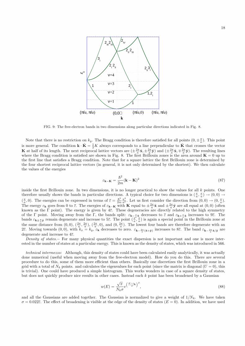
electronic structure electronic structure of selected ... · structure). electronic structure of...
TRANSCRIPT
1
I. SYLLABUS AND INTRODUCTION
The course is taught on basis of lecture notes which are supplemented by the textbook Ashcroft and Mermin. Somepractical information:
• Professor: Michel van Veenendaal
• Office: Faraday West 223
• Tel: 815-753-0667 (NIU), 630-252-4533 (Argonne)
• e-mail: [email protected]
• web page: www.niu.edu/ veenendaal
• Office hours: I am at NIU Tu/Th. Feel free to walk into my office at any time. You can always make anappointment if you are worried that I might not be there. Official office hours will be established if you feel thatthe “open door” policy does not work.
• Prerequisites: there are no official prerequisites for the course. However, a knowledge of quantum mechanics atthe 560/561 level is recommended. In addition, it makes a lot of sense to have taken Solid-State Physics I (566).Mathematical concepts that will be used are calculus, vector algebra, Fourier transforms, differential equations,linear algebra (in particular matrices and eigenvalues problems).
• Homework: several homework sets will be given. They will be posted on the web site.
• Midterm: one midterm will be given.
• Attendence: There is no required attendence.
• Additional further readingF. Wooten, Optical Properties of Solids (Academic Press, New York, 1972).
CONTENTS
• Background: A sort background and history of solid-state physics is given.
• Electronic structure: The lecture notes reverse the order of some of the topics the way they are usually presented.Ashcroft and Mermin (AM) start out with the free electron model and show that it fails and give then avery extended description of crystal structures. The course starts out with electronic structure focusing onsimple systems, such as one-dimensional chains. Although not very realistic, the concepts are much more easilyintroduced in one dimension, since it avoids many complications due to the crystal structure. The tight-bindingand the nearly-free electron model will be introduced and compared. After obtaining a good feeling for theimportant aspects of a solid, some concepts from 566 will be briefly recapitulated (Bloch theorem, crystalstructure).
• Electronic structure of selected materials Several materials will be discussed in detail, such as alkali metals,trivalent metals, transition metals, semiconductors, rare earths.
• Optical properties of materials. The optical properties of materials is discussed using the ideas of polarizationand oscillators. The optical spectra for simple metals, such as aluminum, noble metals (Cu, Ag, Au), andinsulators are described.

2
II. BACKGROUND
From Hoddeson, Braun, Teichamnn, Weart, Out of the crystal maze, (Oxford University Press, 1992).
Obviously, people have been interested in the proporties of solids since the old ages. The ancient Greeks (andessentially all other cultures) classified the essential elements as earth, wind, air, and fire or in modern terms: solids,liquids, gases, and combustion (or chemical reactions in general). Whole periods have been classified by the abilityto master certain solids: the stone age, the bronze age, the iron age. And even our information age is based fora very large part on our ability to manipulate silicon. Many attempts have been made to understand solids: fromGreek philosophers via medieval alchemists to cartesian natural philosophers. Some macroscopic properties could beframed into classical mechanics. Optical conductivity in solids was worked out in the theories of Thomas Young andJean Fresnel in the late eighteenth and early nineteenth century. Elastical phenomena in solids had a long history.Macroscopic theories for electrical conductivity were developed by, e.g. Georg Ohm and Ludwig Kirchhoff. Anothergood example of a mechanical model for a solid are the theories of heat conductivity developed in the early nineteenthcentury by Joseph Fourier. Franz Ernst Neumann developed a mechanical theory for the interaction between elasticityand optics, allowing him to understand anisotropy in materials such as the birefringence that occurs when an isotropicmedium is subjected to pressure or uneven heating.
Another important ingredient to understanding solids is symmetry. Already in 1690, it was suggested by Huygensthat the regular form of solids in intricately related to their physics. The first scientific theory of crystal symmetrywas set up by Rene-Just Hauy in 1801-2, based on atomistic principles. This was extended upon by mineralogistChristian Samuel Weiss, who, however, completely rejected the atomistic approach. He introduced the concepts ofcrystallographic axis. The crowning achievement is the classification by Auguste Bravais that the are only 14 waysto order a set of points so that the neighborhood of any individual lattice point looks the same. In 1901, WoldemarVoight published his book on crystallography classifying the 230 different space groups (and was shocked by the largenumber).
Another important nineteenth century development is the reemergence of the atomistic theories. The success ofcontinuum theories (classical mechanics, electricity and magnetism, thermodynamics) had pushed atomistic thoughtto the background, in particular in physics (remember the trials and tribulation Ludwig Boltzmann went through inthe acceptance of his statistical approach to thermodynamics which was often considered a nice thought experiment,but hopelessly complicated). However, chemical reactions clearly indicated the discrete nature of matter.
A microscopic theory proved elusive until the advent of quantum mechanics in the early twentieth century. Quantummechanics is crucial in understanding condensed matter. For example, gases can be reasonably well described in aclassical framework due to their low density. This means that we do not require quantum (Fermi-Dirac) statistics andwe do not have to deal with atomic levels.
Theories started accelerating after the discovery of the electron by J. J. Thompson and Hendrik Lorentz (and mindyou, Lorentz and Zeeman determined the e/m ratio before Thompson). The classical theory of solids essentiallytreats a solid as a gas of electrons in the same fashion as Boltzmann’s theory of gases. This model was developedby Paul Drude (who, inexplicably, committed suicide at each 42, only a few days after his inauguration as professorat the University of Berlin). The theory was elaborated by Hendrik Lorentz. Although a useful attempt, the use ofMaxwell-Boltzmann statistics as opposed to Fermi-Dirac statistics leads to gross errors with the thermal conductivityκ and the conducivity σ off by several orders of magnitude. The theory gets a lucky break with the Wiedemann-Franzlaw that the ratio κ/σ is proportional to the temperature T . (It is not quite clear to me why AM wants to start outwith an essentially incorrect theory, apart from historic reasons. . . Then again, we also do not teach the Ptolemeansystem anymore). However, it was very important in that it was one of the first microscopic theories of a solid.
Early attempts to apply quantum mechanics to solids focused on specific heat as measured by Nernst. Specificheat was studied theoretically by Einstein and Debye. The difference in their approaches lies in their assumptionon the momentum dependence of the oscillators. Einstein assumed one particular oscillator frequency representingoptical modes. Debye assume sound waves where the energy is proportional to the momentum. Phonon dispersioncurves were calculated in 1912 by Max Born and Theodore von Karman. However, again, this can again be done fromNewton’s equations.
However, further progess had to weight the development of quantum statistics which were not developed untill1926. In the meantime, the number of experimental techniques to study condensed matter was increasing. In 1908,Kamerlingh-Onnes and his low-temperature laboratory managed to produce liquid Helium. This led to the discoveryof superconductivity in mercury (and in some ways the onset of “big” physics).
After discussions with Peter Paul Ewald in 1912, who was working on his dissertation with Sommerfeld on opticalbirefringence, Max von Laue successfully measured the diffraction of X-rays from a solid. The experiments wereinterpreted by William Henry Bragg and his son William Lawrence opening up the way for x-ray crystal analysis.
In 1926-7, Enrico Fermi and Paul Dirac established independently a statistical theory that included Wolfgang

3
Pauli’s principle that quantum states can be occupied by only one electron. This property is inherently related to theantisymmetry of the wavefunctions for fermions. In 1927, Arnold Sommerfeld attempted a first theory of solids usingFermi-Dirac statistics. It had some remarkable improvements over the Drude-Lorentz model. The specific heat wassignificantly lower due to the fact that not all electrons participate in the conductive properties, but only the oneswith the highest energies (i.e. the ones close to the Fermi level). However, the model still completely ignores the effectof the nuclei leading to significant discrepancies with various experiments including resistivity. Werner Heisenbergalso had an interest in metals and proposed the problem to his doctoral student Felix Bloch. The first question thathe wanted Bloch to address was how to deal with the ion in metals? Bloch assumed that the potential of the nucleiwas more important that the kinetic energy. A tight-binding model as opposed to Sommerfeld’s free-electron modeland ended up with the theorem that the wavefunction can be written as ψ = eik·ru(r), plane wave modulated by afunction that has the periodicity of the lattice. Another important development Rudolf Peierls and Leon Brillouinwas the effect of the periodic potential in the opening of gaps at particular values of the momentum k, now known asBrillouin zones.
III. THE ELECTRONIC STRUCTURE
IV. TIGHT-BINDING METHOD
AM Chapter 10
A solid has many properties, such as crystal structure, optical properties (i.e. whether a crystal is transparent oropaque), magnetic properties (magnetic or antiferromagnetic), conductive properties (metallic, insulating), etc. Apartfrom the first, these properties are related to what is known as the electronic structure of a solid. The electronicstructure essentially refers to the behavior of the electrons in the solid. Whereas the nuclei of the atoms that form thesolid are fixed, the electronic properties vary wildly for different systems. Unfortunately, the electronic structure iscomplicated and needs to be often approximated using schemes that sometimes work and at other times fail completely.The behavior of the electrons is, as we know from quantum mechanics, described by a Hamiltonian H . In general,this Hamiltonian contains the kinetic energy of the electron, the potential energy of the nuclei, and the Coulombinteractions between the electrons. Especially, the last one is very hard to deal with. Compare this with a runningcompetition. For the 100 m, the runners have their own lane and the interaction between the runners is minimal.One might consider each runner running for him/herself (obviously, this is not quite correct). However, for largerdistances, the runners leave their lanes and start running in a group. We can no longer consider the runners asrunning independently, since they have to avoid each other, they might bump into each other, etc. This is a muchmore complicated problem. The same is true for solids. In some solids, we can treat the electrons as being more or lessindependent. In some solids, we have to consider the interactions between the electrons explicitly. For the moment,we will neglect the interactions between the electrons, even though for some systems, they can turn the conductiveproperties from metallic to insulating. Systems with strong electron-electron interactions are an important (and stilllargely unsolved) topic in current condensed-matter physics research. The enormous advantage is that we do not havea problem with N particles (where N is of the order of 1023), but N times a one-particle problem. Of course, thisis what you were used to so far. You probably remember the free-electron model (to which we will return later on).First, the bands were obtained (pretty easy since Ek = ~
2k2/2m), and in the end you just filled these eigenstates upto the Fermi level. So far, you might not have realized that this was actually an approximation. This is the type ofsystem we will be considering at the moment. So we are left with a Hamiltonian containing the kinetic energy of theelectron, the potential to the nuclei, and some average potential due to the other electrons in the solid.
In 666 (formerly known as 566), the nearly free-electron model was treated. This is essentially an extension onthe quantum-mechanical model of particles in a box with the periodic potential of the nuclei added later. We willcome back to that in a while, but we start with a model that puts in the atoms explicitly (known as the tight-bindingmodel). This allows us to start thinking about the crystal immediately, instead of putting it in as some afterthought.Crystal can be very complicated, so let us start with something simple: a chain of atoms. Although some materialscan indeed be described as a one-dimensional chain, we are more interested in the concepts, which are very similarin any dimension. Unfortunately, even a chain is rather complicated to start out with, so let us begin with just twoatoms and later add more atoms to it to form the chain. Let us also consider the simplest system: a system ofHydrogen-like atoms (again not very practical, since Hydrogen forms H2 molecules at room temperature, but still amodel often used in theoretical physics). For each site, we only consider one orbital (in our Hydrogen example, thiswould be the 1s orbital). So in total, we have two orbitals ϕ1(r) and ϕ2(r), since we have two sites. However, thiscreates the impression that we have two different orbitals, whereas we only have one type of orbital but located attwo different sites. We can therefore also write ϕ(r − R1) and ϕ(r − R2), where ϕ(r) is the atomic orbital at the

4
origin. With two orbitals in our basis set, we have a total of four matrix elements
ε =
∫
drϕ∗(r −R1)Hϕ(r −R1) =
∫
drϕ∗(r −R2)Hϕ(r −R2) (1)
and
t =
∫
drϕ∗(r −R1)Hϕ(r −R2) =
(∫
drϕ∗(r −R1)Hϕ(r −R2)
)∗, (2)
where we use vector notation to allow easy generalization to arbitrary dimension even though we are considering onlyproblems in one dimension for the moment. In the end, we only have two parameters ε and t. Note that for ε the twomatrix elements are equivalent, since the on-site energy does not depend on the position in space (or, for an Hydrogenatom, ε = −13.6 eV, no matter where you put it in space. The origin (R=0) is only chosen for convenience). For t,the matrix elements are just each others conjugate. t is known as the tranfer matrix element or hopping integral. Letus take t to be a real number (which it is for Hydrogen atoms, since everything is real). We can also write this in abra-ket notation
ε = 〈R1|H |R1〉 = 〈R2|H |R2〉 (3)
t = −〈R1|H |R2〉 = −〈R2|H |R1〉, (4)
where Ri〉 denotes the atomic wavefunction at site Ri. For s-like orbitals, the matrix element would be negative, so twould be a positive number. This allows us to write the Hamiltonian for the two orbitals in the basis set as a matrix
H =
(
ε −t−t ε
)
. (5)
Any vector can now be written as a linear combination of |R1〉 and |R2〉, i.e. |ψ〉 = a1|R1〉 + a2|R2〉. We would liketo solve the Schrodinger equation
H |ψ〉 = E|ψ〉. (6)
We can split this out into different components as
〈Ri|H |ψ〉 = E〈Ri|ψ〉, (7)
with i = 1, 2. There is a complication in that the overlap matrix elements S = 〈R1|R2〉 =∫
drϕ∗(r−R1)ϕ(r−R2) 6= 0.Taking this into account, we obtain
(
ε −t−t ε
)
|ψ〉 =
(
1 SS 1
)
|ψ〉 (8)
Note that 〈R1|R1〉 = 〈R2|R2〉 = 1. The eigenvalues can be found by solving the determinant
∣
∣
∣
∣
ε−E −t−ES−t−ES ε−E
∣
∣
∣
∣
= 0. (9)
This gives the equation
(ε−E)2 − (−t−ES)2 = 0 ⇒ ε−E = ±(−t−ES) ⇒ EB/AB =ε± t
1 ∓ S. (10)
The calculation becomes simpler if we forget about the overlap between the orbitals, which we will do in the remainder,and take S = 0. This gives EB/AB = ε∓ t. The eigenstates are also easily obtained and are
|ψB/AB〉 =1√2(|R1〉 ± |R2〉). (11)
Note that for 〈R1|H |R2〉 < 0 the bonding (B) combination is the lowest (the antibonding (AB) is the lowest for〈R1|H |R2〉 > 0). An electron spends an equal amount of time on atom 1 as it does on atom 2, as it should, becausethere is atom 1 is equivalent to atom 2. In the bonding orbital, the wavefunction is a lot smoother (note thatthe anti bonding orbital has a node between the two atoms). This reduces the kinetic which is proportional to the

5
FIG. 1: The eigenvalues of a linear chain of 2, 5, 9, 15, 100 atoms with a hopping matrix element t between neighboring atoms.
gradient of the wavefunction through to the ∇2ψ term in the Hamiltonian. These are the typical bonding-antibondingcombinations of a H2 molecule. Each atom contributes one electron. The two electrons will go into the bonding orbital,giving
|ψB↑ψB↓〉 =1
2(|R1 ↑ R1 ↓〉 + |R1 ↑ R2 ↓〉 + |R2 ↑ R1 ↓〉 + |R2 ↑ R2 ↓〉), (12)
where we can put two electrons in the bonding orbital due to the spin degree of freedom. Note that the probability offinding the two electrons on the same atom equal that of finding one electron on each atom. This would be surprisingif electrons really interacted strongly with each other. However, we neglected that.
Obviously, this is not much of a solid. However, it is straightforward to extend this procedure to chains of arbitrarylength N . Let us take the atoms on a chain to be numbered 1, 2, 3, · · · , N . General wavefunctions for N sites canthen be written as
ψ(r) =∑
R
aRφ(r −R) or |ψ〉 =∑
R
aR|R〉. (13)
Again, we want to solve the Schrodinger equation H |ψ〉 = E|ψ〉. For the R′’th component, we obtain
〈R′|H |ψ〉 = E〈R′|ψ〉 ⇒∑
i
〈R′|H |R〉aR = E∑
R
〈R′|R〉aR = EaR′ , (14)
where we have assumed 〈R′|R〉 = δR,R′ . We can write this in matrix form as
H11 · · · H1N
. .HN1 · · · HNN
a1
.
.aN
= E
a1
.
.aN
, (15)
where Hij = 〈Ri|H |Rj〉. As before, we have Hnn = ε. If atoms are on neighboring sites, we have Hn,n+1 = −t. Inprinciple, Hn,n+2. Hn,n+3, etc. are nonzero (known as next-nearest neighbor and next-next nearest neighbor hoppingmatrix elements), but we will take them zero for simplicity. This gives a matrix
H =
ε t 0 0 · · ·t ε t 0 0 · · ·0 t ε t 0 0 · · ·0 0 t ε t 0 0 · · ·· · · 0 0 t ε t 0 0 · · ·
· · · 0 0 t ε t 0 0 · · ·. . . .
(16)
Although, not easily solvable by hand, the energies can be found using some computer program that solves eigenvalueproblems. For different lengths N , the eigenvalues are given in Fig. 1. We have taken the constant shift ε = 0. Theeigenvalues En with n = 1, · · · , N are ordered and plotted as a function of (n− 1)/(N − 1), i.e. from 0 to 1. As wehave seen before, for N = 2, the eigenvalues are ±t. However, if we increase the the length of the chain, we see thatthe eigenvalues approach a continuous curve. The extrema of the curve are ±2t. The question is what is this curveand can we obtain this curve in different fashion apart from solving the matrix by brute force?
First, we have to realize that we want to study bulk systems or systems that are essentially infinity. The study ofsurfaces is a whole field in itself but not our focus at the moment. For small chains the number of atoms close tothe edge of the chain is relatively large. So we can study a large system, but we can also introduce a mathematicaltrick. Note, that none of the atoms in the chain is equivalent, since they all have a different distance to the end ofthe chain. However, if we connect the two ends of the chain to each other, all the atoms become equivalent. This isknown as periodic boundary conditions. Although, this is essentially a mathematical trick, in some systems this is

6
FIG. 2: The lines give the values of eikx and e(k+K)x as a function of x. We have taken k = 0.3π and K = 2π. The dotsindicate the values at the atomic positions. Note that the Fourier transform only includes these values.
physically realized. The best known example would be a benzene ring consisting of six carbon atoms. However, intwo and three dimensions, this is more difficult to realize. In two dimensions, the system would be a torus (whichcould be achieved, maybe, with a carbon nanotube), but in three dimension, it is impossible to realize. Let us goback to the diatomic molecule. Applying periodic boundary condition implies that 1 is connected to 2, but 2 is againconnected to 1. This leads to a doubling of the transfer matrix element, giving a Hamiltonian:
H =
(
ε −2t−2t ε
)
. (17)
The eigenvalues are E1,2 = ∓2t. Note that this is equal to the extrema in the continuous curve we obtained for largeN . This is a significant difference from the ±t, we obtained earlier. We could expect that, because all atoms in the“chain” are at the end of the chain. For larger
H =
ε t 0 0 · · · 0 tt ε t 0 0 · · · 0 00 t ε t 0 0 · · ·0 0 t ε t 0 0 · · ·· · · 0 0 t ε t 0 0 · · ·
· · · 0 0 t ε t 0 0 · · ·. . . .
0 0 . . 0 t ε tt 0 . . . 0 t ε
(18)
Obviously, whenN is very large (and number of atoms are generally very large numbers), this one extra matrix elementwill not affect the majority of the eigenvalues, so the eigenvalues with and without periodic boundary conditions shouldvirtually identical. If you solve this matrix you find out that the eigenvalues always lie on the curve that is obtainedwhen N → ∞.
So what is missing here? The essential ingredient is translational symmetry. Although we are all attached to realspace, it is the periodicity that is really important. When there are milemarkers along the road, you do not saythere is a mile marker at 1 mile, and one a 2 miles, and one at 3 miles. You say there is a mile marker every 1mile. In a more mathematical term, we should be considering Fourier transforms. The quantity that is related tospace by Fourier transform is momentum (the other important dimension is time, which is related to frequency byFourier transform, which, in quantum mechanics is directly related to energy). In free space, space is continuous, andtherefore the momentum is continuous as well. Conservation of momentum in classical mechanics is inherently relatedto the translational symmetry of space. When we go to a solid, the translational symmetry of space is no longercontinuous, but related to the interatomic distances and therefore discrete. We applied periodic boundary conditionsso we need to satisfy:
eik(x+L) = eikx (19)
where the length of the chain is L = Na, with a the distance between the atoms. This means is we displace ourselvesby L (the lenght of the chain), we end up at the same position due to the periodic boundary conditions. This impliesthat
kL = ±2nπ ⇒ k = ±2nπ
L, (20)

7
where n is an integer. This would lead to an infinite amount of wavenumbers k. This is not entirely correct. Beforedoing a Fourier transform, we had N orbitals, one for each site. After the Fourier transform, we should still end upwith the same number of states. Therefore, since we have positive and negative numbers, the maximum n is N/2.The allowed k values are therefore
k = 0,±2π
L,±4π
L, . . . ,±π
a. (21)
So we only have k values in the region [−πa ,
πa ]. You might wonder what happened to all the other k values. From
a point a view of periodicity, they are exactly equivalent. Figure 2 shows a comparison between eikx and ei(k+2π/a)x
(where for the example k is taken 0.3π). Although the function are of course different, the have the same values atthe sites of the atoms (indicated by the blue dots). However, you might remember from Fourier analysis that youoften need all k values to build special functions (e.g. a square or a delta function) and there might be structure inthe wavefunction that Fourier components with a larger k value. However, the k is only related the periodic part ofthe wavefunction. These smaller structures are related to the atomic part of the wavefunction
ϕk(r) =1√N
∑
R
eik·Rϕ(r −R). (22)
Note that the Fourier transform only includes the values of the exponentials at the atomic positions. Therefore, anyk+ 2πn, with n and integer, is equivalent to k. Essentially, this is a unitary transformation of N wavefunction in realspace to a k dependent basis. We can also inverse this procedure
ϕ(r −R) =1√N
∑
k
e−ik·Rϕk(r). (23)
We can also write this in bra-ket notation
|k〉 =1√N
∑
R
eik·R|R〉 and |R〉 =1√N
∑
k
e−ik·R|k〉. (24)
We now want to understand what the Hamiltonian looks like in this new basis set. Let us first rewrite the Hamiltonianin bra-ket notation in real space. Note that
|Ri〉〈Rj | =i→
0..010.
(0, 0, · · · , 0, 1, 0, · · · )↑j
= i→
. . .· · · 0 0 0 · · ·· · · 0 1 0 · · ·· · · 0 0 0 · · ·
. . .
(25)
↑j
using this we can rewrite the matrix in Eqn. (18)
H =∑
R,R′
|R′〉〈R′|H |R〉〈R| = −t∑
Rδ
|R + δ〉〈R|, (26)
where δ is a vector connecting R to its nearest neighbors (the atoms left and right of the atom in a chain). TheFourier transform can be made by inserting the definitions into the Hamiltonian:
H = = −t∑
Rδ
1
N
∑
k,k′
e−ik·(R+δ)|k〉〈k′|eik′·R (27)
= −t∑
k,k′
(
1
N
∑
R
ei(k′−k)·R)(
∑
δ
e−ik·δ)
|k〉〈k′| (28)
=∑
k,k′
δk,k′εk|k〉〈k′|. (29)

8
-2
-1
0
1
2
ε k /t
k
−π/a π/a−π/2a π/2a0
FIG. 3: The eigenenergies for a single tight-binding band εk = −2t cos k as a function of k.
We see that the Hamiltonian is diagonal in k due to the delta function. The diagonal matrix elements (which aredirectly the eigenvalues) are given by
εk = −t∑
δ
e−ik·δ. (30)
The nearest-neighbor vectors for a chain in the x-direction are given by δ = ±ax, where x is a unit vector in thex-direction.
εk = −t(eika + e−ika) = −2t coska, (31)
where k = kx. Since goes from −πa to π
a , the eigenvalues lie on a cosine between −2t and 2t, see Fig. 3.
V. NEARLY FREE-ELECTRON MODEL
AM Chapter 9
In free space in the Schrodinger equation is given by
− ~2
2m∇2ψ(r) = Eψ(r). (32)
The solution is well known and the eigenfunction are simple plane waves
ψ(r) =1√Veik·r, (33)
where V is the size of the system. The eigenvalues are
εk =~
2k2
2m(34)
Again, we can apply periodic boundary condition, see Eqn. (21), giving
ki = ±2πn
Lwith n integer. (35)
Note that so far there is no restriction on the k values to the range [− πa ,
πa ]. The only thing we have done so far is
put the particles in a box, which is not yet a solid. The system becomes a solid by introducing the potential U(r) due

9
to the nuclei that are arrange in a periodic structure. In general, we can express any arbitrary potential in a Fourierseries
U(r) =∑
k
Uke−ik·r. (36)
However, we want to impose that the potential satisfies the periodicity of the lattice. Therefore, the potential shouldbe equivalent when moving to a different lattice site by the vectors R that indicate the lattice sites:
U(r + R) =∑
k
Uke−ik·(r+R) = eik·RU(r). (37)
This is not going to work for any arbitray wavevector k. The vectors K that satisfy this are known as reciprocallattice vectors
eiK·R = 1. (38)
These vectors return again and again since they are intimately related to the translational symmetry of the crystal.We will discuss in more detail later on how to obtain these reciprocal lattice vectors and discuss various cases fordifferent crystals. (and you might remember them from 566/666 or x-ray diffraction). Let us just satisfy ourselvesthat these vectors exist and only consider the case of one dimension
eiKa = 1 ⇒ K = ±2πn
a. (39)
Note that since a is much smaller than L, the K are much larger the separation between the k values. In general, theperiodic potential is therefore given by
U(r) =∑
K
UKe−iK·r. (40)
The matrix elements between different running waves are given by
〈k′|U |k〉 =∑
K
1
V
∫
dxe−ik′·rUKeiK·reik·r =
∑
K
UK
1
V
∫
dre−i(k′−K−k)·r =∑
K
UKδk′,k+K. (41)
In bra-ket notation, we can write the potential as
U =∑
kK
UK|k + K〉〈k| (42)
This has the importance consequence that a running wave with wavevector k is coupled to the running waves withwavevectors k±2πn/a with n = 0, 1, 2, 3, · · · , see Fig. 4. However, this also means that k is no longer a good quantumnumber. The periodic potential reduces the k values that are good quantum numbers. Although we are free to choosethe k values, generally the region [−K/2,K/2] = [−π/a, π/a] is chosen. The wavevectors inside this region do notcouple to each other with the periodic potential. In addition, any wavevector outside this region is coupled to oneinside by a reciprocal lattice vector K. The allowed k values are therefore equivalent to those found in Eqn. (21)when discussing the tight-binding model.
Since only the k values separated by a reciprocal lattice vector K couple, we can write the eigenfunctions as a linearcombination of these running waves
ψk(r) =∑
K
ck−Kei(k−K)·r, (43)
where ck−K is a coefficient. For each k, we find a set of coupled equations
εk−Kck−K +∑
K′
UK′ck−K+K′ = Eck−K. (44)
Note that this reproduces to E = εk−K in the absence of a periodic potential.

10
ε k
kπ/a−π/a−2π/a 0 2π/a
FIG. 4: The scattering of electrons between different running waves eikx due to a periodic potential resulting from nuclei in achain at a distance a from each other. The potential couples k values with each other that are K = ±2πn/a apart. The bluearrows show this scattering for an arbitrary k value (Note that only three k points are included). The red arrow shows theparticular case for k = ±π
a. This is a Bragg reflection and the electrons scatters to k = ∓ π
awhich has exactly the same energy
εk.
This model is known as the nearly-free electron model and is generally use only in the case the the periodic potentialis weak (such as K, Na, and Al metals). However, even a weak potential can have a large influence if the energyseparation of the states that if couples is small (or even zero). For the energy difference to be zero we require
εk = εk−K ⇒ k2 = (k −K)2 = k2 − 2k · K +K2, (45)
or
k · K =1
2K2. (46)
Some of you might recognize this as the Laue condition for x-ray diffraction (which, of course is equivalent to the Braggcondition). In principle, this should not be a surprise. X-rays are scattered by a lattice through repeated interactionwith the nuclei. The same applies to electrons. In one dimension, k and K are either parallel or antiparallel and wefind k = ± 1
2K.Let us consider K = 2π/a, for which k = K/2 = π/a should have the same energy as k −K = −π/a,which is indeed correct. The effect are therefore strongest close to the k values indicated by the dotted lines in Fig. 4.In this region, we can neglect the coupling to other running waves if |εk − εk−K| � U . We are then left with solvingthe determinant
∣
∣
∣
∣
εk −E UK
U∗K εk−K −E
∣
∣
∣
∣
= 0. (47)
This leads to the quadratic equation
(εk −E)(εk−K −E) − |UK|2 = 0, (48)
which has the solutions
E =εk + εk−K
2±
√
(
εk − εk−K
2
)2
+ |UK|2. (49)
In the limit that εk ∼= εk−K, we obtain
E = εk ± |UK|. (50)

11
Ε k
k
π/a−π/a−2π/a 0 2π/a
2U
FIG. 5: Calculation of the bands in a nearly-free electron model. Shown are the energies εk and εk+K with K = ± 2π
a. The
calculated nearly-free electron bands are shown for the region [−K/2, K/2] = [− π
a, π
a]
We see that an energy gap opens at the k = ± 12K. We can also verify that in this limit
∂E
∂k=
~2
m(q − 1
2K), (51)
i.e. the derivative is zero on the Bragg planes and the bands are therefore flat. (Not entirely surprising since we justdemonstrated that a gap opens, so the bands must be either in a maximum or a minimum).
We can extend this procedure to include additional reciprocal lattice vectors K. Let us consider the situation inone dimension for K = 0 and K± = ±π
a . We can also use the following properties of the potential. Since the potentialis real, we have
U−K = U∗K. (52)
If in addition, we have inversion symmetry (meaning that the system is unchanged when r → −r, which is the casefor a linear chain), we also have
U−K = UK = U∗K. (53)
Using this we can write down the Hamiltonian.
H =
εk UK UK
UK εk−K− U2K
UK U2K εk−K+
. (54)
The results are given in Fig. 5. Note that the energies εk−K± = ~2(k −K±)2/2m look in the region [−K/2,K/2] as
parabolas centered around K±. The eigenvalues of H can be easily solved numerically. The values for Ekn, wheren = 1, 2, 3 is the bandindex are plotted in the region [−K/2,K/2]. We have taken UK = U2K . This is known as thereduced-zone scheme, see AM Fig. 9.4). This is the scheme commonly used is the scientific literature. Figure 9.4also shows the extended-zone scheme and the repeated-zone scheme. In particular, the extended-zone scheme looksnatural at first. It looks like the original parabola with gaps opened at the reciprocal lattice vectors K. However,this clings too much to the free-electron like picture and in some sense is slightly misleading. It is important to notethat in a chain of N atoms, there are only N k-values that are good quantum numbers. Convention dictates thatthese N k-values are chosen in the region [−K/2,K/2]. This region is known as the first Brillouin zone. All theother k-values are not good quantum number. For example, k = 2.3π/a is not a good k value since it is coupledby the periodic potential to k = 0.3π/a. This directly implies that we have more eigenstates than k-values. Thisis why there is another quantum number, the band index n. All eigenstates Ekn are identified by the value of k in

12
ψ
xk=0, n=1
k=π/a, n=1
k=π/a, n=2
k=0, n=2
FIG. 6: The wavefunction of the nearly-free electron eigenstates for four eigenvalues E0,1, E πa
,1, E πa
,2, and E0,2. We haveassumed UK < 0 and U2K > 0.
the region [−K/2,K/2] and the band index n. Because of the mixing, we can no longer identify eigenstates with thefree-electron bands. Even at k = 0, we have, for the lowest eigenfunction in Fig. 5,
|Ek=0,1〉 = a|k〉 −√
1 − a2(|k −K−〉 + |k −K+〉), (55)
where a ∼= 1 (actually a = 0.9978 for the example in the figure). Indeed close to |k〉, but still mixed with |k ±K±〉.The repeated-zone scheme has its uses from time to time, as long as you keep in mind that it just repeats the sameinformation as is already contained in the first Brillouin zone and nothing new is added.
VI. COMPARISON OF RESULTS FOR TIGHT-BINDING AND NEARLY-FREE ELECTRON MODEL
In this section, we will compare the results from tight-binding and the nearly-free electron model. At first, thislooks like a pointless excersize. For tight-biding we find a single band given Ek = −2t coska. For the nearly-freeelectron model we have several bands which originate from free electron parabolas. Although, we are not going tomake the claim that the two are exactly equivalent, they have more in common that you might think at first sight. Thetight-binding model starts from atomic states which include the potential of the nucleus fully and then starts addingthe kinetic energy due to the delocalization of the electrons when the solid is formed. The nearly-free electron modelstarts from completely delocalized electron and starts adding the effect of the potential of the nuclei. Somewherealong the way to two must have something in common. (They will never be entirely equivalent, since the treatment ofthe potential in the nearly-free electron is somewhat oversimplified. The inclusion of only two Fourier compoments,UK and U2K , is obviously insufficient to describe the much more complicated shape of the potential.
Let us start by looking at the eigenfunctions in the nearly-free electron model. Let us start with the one with thelowest energy. The eigenfunction is given in Eqn. (55). This gives a wave in real space for k = 0 and n = 1,
ψ0,1(x) =1√L
(a− 2√
1 − a2 cosKx). (56)
In the case that a = 1 (i.e., the limit U = 0), we just obtain that psi0,1 = 1√L
constant throughout the system. The
higher-order oscillation are a result of the (small) mixing in of the K± terms.Effect are more drastic around k = K±/2. Let us take k = K+/2 = π
a . Here we obtain mixing of the free-electronstates εk and εk−K+/2, as we have solved in Eqn. (47) (we can neglect εk+K/2 which is at higher-energies). Thewavefunction are
ψπ2
,i(x) =1
2√L
(ei πa
x ∓ sgn(UK)ei πa
x). (57)
with i = 1, 2. The wavefunctions depend on the sign of the coupling. Let us consider the situation UK < 0, shown in

13
Fig. 116, which gives
ψπ2
,i(x) =
√
2L cos π
ax
i√
2L sin π
ax(58)
We see that ψπ2
,1(x) has extrema on the positions of the nuclei, whereas ψ π2
,2(x) has nodes on the positions of thenuclei. This is reminescent of atomic physics: s orbitals have their maxima at the nucleus, whereas, for examplethe px orbital has a node at the nucleus. From this we can understand one origin of the discrepance between ourtight-binding and nearly-free electron calculation. In our tight-binding calculation, we only included s orbitals, so weonly get one bandw hich resembles the lowest band of the nearly-free electron calculation, but not the higher-lyingband. On the other hand, we also see that the effect of folding the free-electron bands is to create “orbital-like”structure related to the nuclei. For the highest energy of the second band (n = 2), the wavefunction has nodes notonly at the nuclei, but also between the nuclei, see Fig. 116.
However, we see that we can create a better connection between the two approaches by including p type orbitals.Let us try to extend our tight-binding approach, following the approach by Slater and Koster, Phys. Rev. B 94, 1498(1954). We adjust Eqn. (22) to allow the inclusion of more orbitals
ϕk,s(r) =1√N
∑
R
eik·Rϕs(r −R). (59)
The dispersion for these states, we found to be
εssk = 2(ssσ) cos k with (ssσ) =
∫
drϕs(r −R′)Hϕs(r −R) (60)
where R and R′ are nearest neigbors and (ssσ) = −t (using the notation by Slater and Koster indicating that thematrix element is between two s orbitals; the σ indicates the type of bonding. There are also π and δ bonding, butthat is not relevant for the discussion here). We can repeat this approach for p orbitals giving
ϕk,p(r) =1√N
∑
R
eik·Rϕp(r −R) (61)
with energies
εppk = 2(ppσ) cos k. with (ppσ) =
∫
drϕp(r −R′)Hϕp(r −R) (62)
This looks similar, but there is an important difference. For typical Hamiltonians H , the matrix elements are negativewhen the positive lobes are pointing to each other. This is always the case for the s orbital which is positive everywhere
· · · (+)(+)(+)(+)(+)(+)(+)(+) · · · , (63)
where (+) schematically indicates an s orbital at a certain site. This is the state found for k = 0 (and energyεk = 2(sσ) < 0). Note that this is positive everywhere just as the nearly-free electron wavefunction for k = 0 andn = 1 in Fig. 116. For k = π
a (and energy εk = −2(sσ) > 0), the exponential changes sign at each site, giving
· · · (+)(−)(+)(−)(+)(−)(+)(−) · · · . (64)
This has nodes between the nuclei, just as the wavefunction for k = πa and n = 1.
The p orbital on the other hand have a node
· · · (−+)(−+)(−+)(−+)(−+)(−+)(−+)(−+) · · · (65)
The convention we choose is that the postive lobe of the p orbital (−+) is in the positive x direction (we can chooseany convention that we like, but in the end it should lead to the same results). In this convention, we see that thepositive lobes are pointing towards the negative lobes. The matrix elements are therefore negative. This also has asa consquence that the solution with the lowest energy is the one where the sign changes for each sites, i.e.
· · · (−+)(+−)(−+)(+−)(−+)(+−)(−+)(+−) · · · (66)

14
However, this looks nice since the positive lobes are pointing towards the positive lobes and the negative lobes arepointing towards the negative lobes. This is essentially the bonding state with no nodes between the nuclei. Thiscorresponds well with the lowest n = 2 nearly-free electrons solution for k = π
a (alternating signs), which also has nonodes between the nuclei. The state with the higher energy is given in Eqn. (65), where there are nodes between thenuclei, comparable to the nearly-free electron wavefunction for k = 0 and n = 2 in Fig. 116.
We can also compare the dispersion. In order to do this, we need to overcome one more hurdle, namely the matrixelements between s and p are not zero,
(spσ) =
∫
drϕs(r −R′)Hϕp(r −R). (67)
The dispersion does not follow a cosine dependence since an s orbital, in our convention, couples differently to theleft and the right
· · · (−+)(+)(−+), (68)
a problem that did not arise when dealing with just s orbitals. Following Eqns. (30) and (31), we find
εspk = (spσ)(eika − e−ika) = 2i(spσ) sin ka. (69)
We now have a basis (ψk,s, ψk,p) giving a matrix
H =
(
εssk εsp
k(εsp
k )∗ εppk
)
(70)
Figure 7 gives a comparison between the lowest two bands (n = 1, 2) in the nearly-free electron model and the s andp tight-binding model. The fit has been done by eye. Although a perfect fit cannot be expected due to the differentapproximations, it is clear that they are giving comparable physics.
Although, at first sight, it might seem surprising that similar physics comes out of a model starting with freeelectrons and a model starting from atomic orbitals. A comparison between tight-binding and nearly-free electronmodel can be given as follows:
tight binding nearly free electronmodel
starting point atomic properties kinetic energy of the electronsbasis functions atomic orbitals plane wavesk = ±n 2π
L periodic boundary conditions periodic boundary conditionsk ∈ [−π
a ,πa ] N atoms give N k values or N
22πL ≤ k ≤ N
22πL periodic potential couples k values
that differ by K = n 2πa
number of bands equals number of atomic orbitals equal number of reciprocal lattice vectorsapproximations neglect orbitals UK = 0 for large K
(71)
However, when you think more of it, in principle it should not make a difference. The starting wavefunctions arejust a basis. If my basis is complete (i.e. you can express any arbitrary wavefunction in your basis, a statement youmight remember from Fourier analysis) then solving the same Hamiltonian should give the same eigenfunction andeigenenergies, regardless of the basis we started with. Differences do arise because we start making approximationsalong the way:
• The free-electron model is beautiful as a basis (exponentials are the foundation of Fourier analysis): they areorthogonal and complete. The tight-binding basis set is more problematic. In principle, the solutions of theHydrogen atom form a complete basis which is orthogonal. However, this is not what we are doing. We aretaking the solution and putting them on different sites. This basis set is not even orthogonal.
• The potential of the nuclei is much better treated in the tight-binding model. There is one important caveat: ingeneral we are not dealing with Hydrogen atom. The potential is treated much more poorly in the nearly-freeelectron model. So far, we have included only two Fourier terms. Obviously, this will give a sinosoidal potentialand not the 1/r potential that one would expect from the nuclei. However, in principle nothing prevents usfrom including all Fourier components. Then again, this defeats the purpose of a nearly-free electron model.
Summarizing, although the nearly-free electron usually takes pride of place in most textbooks over the tight-bindingmodel (in that it is usually treated in an earlier chapter), the tight-binding model wins out in practicality. Tight-binding is often used in the scientific literature. The electronic structure is nowadays generally calculated with complex

15
k
−π/a π/a−π/2a π/2a0
E
FIG. 7: Comparison of the two bands lowest in energy (n = 1, 2) in a nearly-free electron with a tight-binding calculationincluding an s and a p orbital.
codes that have been developed over many years. However, one often would like to use the output of such calculationsas the input for other calculations (for the experts, for example, many-body calculations or molecular dynamics). Thisis usually done by making a tight-binding fit to the more sophisticated electronic structure calculations. Nearly-freeelectron models are used much less often (typing in tight-binding on Physical Review online yielded more 3500 papers,whereas nearly-free electron gave less than 300 papers). One of the reasons is that it works well for only a few systems,usually involving s and sometimes p orbitals. One might actually wonder why it works at all. One needs that thenucleus is very well screened. One has to realize that most electrons in a solid are very strongly bound to the nucleusand only the electrons in the outer shells really form bands. However, this inner shell electrons can effectively screenthe nucleus. They are effectively a negative charge compensating the positive charge of the nucleus.
VII. FORMALIZATION: BLOCH THEOREM
AM Chapter 8
In the chaper on the nearly-free electron model we saw that the wavefunction can be written as, copying Eqn. (43),
ψk(r) =∑
K
ck−Kei(k−K)·r. (72)
Since the exponentials form a complete basis set (which means we should be able to express any function in them),this is a general statement. We can therefore express all eigenstates with eigenenergies Enk in this fashion. We alsosaw that k is a good quantum number in a crystal. Let us therefore separate the part related to k
ψnk(r) = eik·r∑
K
cnk−Ke−iK·r = eik·runk(r) with unk(r) =
∑
K
cnk−Ke−iK·r. (73)
This shows that the eigenfunction can be expressed in a plane-wave part eik·r and a function unk(r). The interestingproperty of the latter is that it has the periodicity of the lattice
unk(r + R) =∑
K
cnk−Ke−iK·(r+R) = unk(r), (74)
since e−iK·R = 1. This is related to the orbital structure that we obtained when folding k values back into the firstBrillouin zone (in one dimension, the region [−K/2,K/2]. An alternative way of expressing Bloch’s theorem is
ψnk(r + R) = eik·(r+R)unk(r + R) = eik·Rψnk(r). (75)

16
That is nice you might say, but what does it physically mean? Let us consider free space. We know that the solutionsare given by plane waves
ψk,free(r) =1√Veik·r. (76)
Free space is uniform. Therefore, we expect that the probability of finding an electron is equal everywhere. This isthe case since |ψk,free|2 = 1/V everywhere (some of you might say that the probability does not have to be constant:we can make wavepackages. This is correct, but you might also remember that wave packages are not eigenstates infree space). However, even though the probability is constant, the wavefunction can still pick up a phase. Under adisplacement τ , we have
ψk,free(r + τ ) =1√Veik·(r+τ ) = eik·τψk,free(r). (77)
In a solid, we do not expect the probability to be uniform in space. On the contrary, it is very natural to expect thatthe probability is higher closer to the nuclei where the electron feel and attractive potential. So we do not expectsomething for an arbitrary vector tau. However, we do expect that the probability is exactly the same when wedisplace ourselves by a lattice vector R. After all, the solid looks exactly the same again. This is the underlyingphysics of Eqn. (75). In a solid, under displament of R, the only change to the wavefunction can be a phase factor.
Does the Bloch theorem also hold for tight-binding wavefunctions that look different from Eqn. (72), see Eqn. (22).Let us check
ϕk(r + R′) =1√N
∑
R
eik·Rϕ(r + R′ −R)
=1√Neik·R′ ∑
R−R′
eik·(R−R′)ϕ(r + R′ −R) = eik·R′
ϕk(r), (78)
which is Bloch’s theorem.
VIII. CRYSTAL STRUCTURES
AM Chapters 4-7
In this section, we will briefly repeat some of the important aspects of the crystal structure. This has been treatedextensively in 566. In the previous sections, we studied a simple one-dimensional chain consisting of one type of atom.Taking this chain along the x-direction, we can build up this chain by taking multiples of a primitive vector that givesthe vector needed to go from lattice site into another
a1 = ax ⇒ R = na1 with n = · · · ,−2,−1, 0, 1, 2, · · · (79)
However, more important for our considerations of the periodic potential was not so much the real space positionof the atoms, but their effect on reciprocal space. This is directly related to the fact that momentum k is a goodquantum number. Translational symmetry of the potential imposed, reproducing Eqn. (82),
eiK·R = 1. (80)
In one dimension this gives reciprocal lattice vectors, which again can be expressed in a unit vector
b1 =2π
ax ⇒ K = nb1 with n = · · · ,−2,−1, 0, 1, 2, · · · (81)
It is easy to see that R and K satisfy the condition eiK·R = 1. In condensed-matter physics, one is dealing moreoften with three-dimensional systems. Again, we can built up a crystal starting from the primitive vectors a1, a2,and a3. For a simple cubic system, these are given by a1 = ax, a2 = ay, and a3 = az. Often however the crystalstructures are more complicated, such as face-centered cubic or body-centered cubic. (This is for a large part relatedto the fact that simple cubic is not close packed. Try obtaining a simple cubic lattice by throwing marbles in a box. . . ). The crystal structures that are built up are called Bravais lattices. Often the primitive vectors are insufficientto generate the crystal lattice and instead of having one atom at the positions R, one has several. Simple examples

17
12
I
3
3
33
3
3
3 32II
2III
2IV
3I
FIG. 8: The first three Brillouin zones for a square lattice.
are graphite, which has a honeycomb lattice and Si and diamond, which have a diamond lattice. However, despitetheir added complexity, one still needs to satisfy the condition eiK·R = 1. This can be done by defining the primitivevectors
b1 = 2πa2 × a3
a1 · a2 × a3. (82)
The vectors b2 and b3 can be obtained by cyclic rotation, i.e 1 → 2 → 3 → 1. Note tha a2 · b1 = 0 and a3 · b1 = 0,since the outer product makes b1 perpendicular to a2 and a3. In addition, a1 · b1 = 2π, and therefore the conditioneiK·R = 1 is satisfied. It is important to remember that for the electronic structure, the most dramatic effects due tothe periodic potential do not happen at the reciprocal lattice vectors K but at the points in reciprocal space wherethe Bragg condition, see Eqn. (46)
k · K =1
2K2, or k · K =
1
2K, (83)
where is K is a unit vector in the direction of K, is satisfied.
IX. FREE ELECTRON IN TWO DIMENSIONS
Let us consider the nearly-free electron model in two dimensions for a square lattice. A square lattice can begenerated by the primitive vectors
a1 = ax and a2 = ay ⇒ R = n1a1 + n2a2. (84)
The reciprocal lattice vectors satisfying eiK·R = 1 are also easily obtained
b1 =2π
ax and b2 =
2π
ay ⇒ K = n1b1 + n2b2. (85)
We will be calculating the electronic structure in the first Brillouin zone. Although we will consider the other Brillouinzones to try to connect to the free-electron model, it is important to get used to working in the first Brillouin withonly the k vectors that are good quantum numbers for the system. Virtually all sophisticated electronic structureprograms work only in the first Brillouin zone. For the one-dimensional chain, the first Brillouin zone was the region[−π
a ,πa ], where the k-points ±π
a satisfy the Bragg condition k = 12K, see Eqn. (83). To find the first Brillouin zone
in two dimensions, we need to find the k points that satisfy the Bragg condition. Obviously, we need to unclude thereciprocal lattice vector K = 0. The next reciprocal lattice vectors are ± 2π
a x and ± 2πa y. This leads to the following
Bragg condition in the x-direction
k · (±x) =1
2
2π
a⇒ kx = ±π
a. (86)
18
ε k
k
(π/a,0)(0,0) (π/a, π/a)(π/a, π/a)
1
1,2I
1
ν=1
ν=2
ν=3
ν=4
3I
2I
2II
2IV
2III
2I2
II
2IV
2III
2II3
I
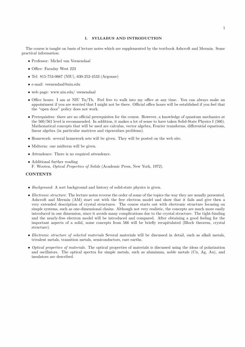
FIG. 9: The free-electron bands in two dimensions along particular directions indicated in Fig. 8.
Note that there is no restriction on ky. The Bragg condition is therefore satisfied for all points (0,± πa ). This point
is more general. The condition k · K = 12K always corresponds to a line perpendicular to K that crosses the vector
K at half of its length. The next reciprocal lattice vectors are (± 2πa x,± 2π
a y) and (± 2πa x,∓ 2π
a y). The resulting lineswhere the Bragg condition is satisfied are shown in Fig. 8. The first Brillouin zones is the area around K = 0 up tothe first line that satisfies a Bragg condition. Note that for a square lattice the first Brillouin zone is determined bythe four shortest reciprocal lattice vectors (in general, it is not only determined by the shortest). We then calculatethe values of the energies
εk−K =~
2
2m(k −K)2 (87)
inside the first Brillouin zone. In two dimensions, it is no longer practical to show the values for all k points. Onetherefore usually shows the bands in particular directions. A typical choice for two dimensions is ( π
a ,πa ) → (0, 0) →
(πa , 0). The energies can be expressed in terms of ε = ~
2
2mπ2
a2 . Let us first consider the direction from (0, 0) → (0, πa ).
The energy εk goes from 0 to ε. The energies of εk−K with K equal to ± 2πa x and ± 2π
a y are all equal at (0, 0) (oftenknown as the Γ point). The energy is given by 4ε. These degeneracies are directly related to the high symmetryof the Γ point. Moving away from the Γ, the bands split: εk−π
ax decreases to ε and εk+ π
ax increases to 9ε. The
bands εk±πay remain degenerate and increase to 5ε. The point (π
a ,πa ) is again a special point in the Brillouin zone at
the same distance from (0, 0), ( 2πa ,
2πa ), ( 2π
a , 0), and (0, 2πa ). The lowest four bands are therefore degenerate with an
2ε. Moving towards (0, 0), with kx = ky, εk decreases to zero. εk− 2πa
(x+y) increases to 8ε. The band εk− 2πa
x/y are
degenerate and increase to 4ε.Density of states.− For many physical quantities the exact dispersion is not important and one is more inter-
ested in the number of states at a particular energy. This is known as the density of states, which was introduced in 566.
technical intermezzo: Although, this density of states could have been calculated easily analytically, it was actuallydone numerical (useful when moving away from the free-electron model). How do you do this. There are severalprocedure to do this, some of them more efficient than others. Basically one discretizes the first Brillouin zone in agrid with a total of Nk points. and calculates the eigenvalues for each point (since the matrix is diagonal (U = 0), thisis trivial). One could have produced a simple histrogram. This works wonders in case of a square density of states,but does not quickly produce nice results in other cases. Instead each k point has been broadened by a Gaussian
w(E) =
√π
Nkσe
(
E−εk
σ
)
2
, (88)
and all the Gaussians are added together. The Gaussian is normalized to give a weight of 1/Nk. We have takenσ = 0.022ε. The effect of broadening is visible at the edge of the density of states (E = 0). In addition, we have used

19
0
1
2
3
4
0 1 2 3 4 5
ρ(Ε)
ε a2
Ε/ ε
FIG. 10: The green line gives the density of states as a function of energy. The red line gives the integrated density of states.The dotted dark-blue line gives the density of states of the band from the first Brillouin zone (indicated by 1 in Fig. 9). Thedotted light-blue gives it integral.
0
1
0 1 2 3 4 5
DO
S
Ε/ ε
FIG. 11: Typical numerical problems in calculating the density of states. Dashed blue line: insufficient k points taken intoaccount in the calculation. Black line: improper treatment of the edges of the Brillouin zone.
Nk = 2002, which gives a nice smooth result. When Nk = 50 is taken, one observes oscillations, see Fig. 11, due to theundersampling of the Brillouin zone. The black line in Fig. 11 shows the effect of an improper treatment of the edgesof the Brillouin zone. The calculation uses only a quarter of the Brillouin zone (only positive k), since the other partsare equivalent. In fact, we really only need 1/8 of the whole Brillouin zone due to symmetry. However, the k points atthe edges are shared by different regions. For example, the k points at the edge of the first Brillouin zone lie for onehalf in the first and for the other half in the second Brillouin zone. When this is not taking into account properly (i.e.by scaling these k points by a factor of 1
2 , one observes spikes in the density of states, see the black line in Fig. 11.
Obviously, these would become irrelevant when Nk → ∞, by for Nk = 1002 they are clearly visible. There exist moreadvanced and efficient methods to calculate the density of states (for example, the tetrahedron method, which ef-fectively interpolates between the different k-points), but for a simple two-dimensional problem this works well enough.
The results are shown in Fig. 10. The end result looks simple: the density of states is constant. Obviously, we

20
could have derived this more easily. However, in general this cannot be done, so this is certainly a useful check tosee whether this routine works properly. Let us derive this density of states analytically. We ignore the spin of theelectron for the moment. Although we have a discrete number of k states, the density is always large enough that
we can approximate this by a continuous function. The amount of k space occupied by one k point is A1 =(
2πL
)2
following from the periodic boundary conditions in Eqn. (21) appplied in both x and y directions. The number of kstates in a certain are can then be obtained by dividing the are by A1. For a free-electron model where the energy is
given by εk = ~2k2
2m , the areas of constant energy are circles. The number of electron inside the circle is given by
N(k) = πk2/A1 = πk2
(
L
2π
)2
=A
4πk2, (89)
where A is the area (i.e. the size) of the system. This number can be easily written in terms of energy
N(E) =A
4π
2m
~2E or n(E) =
N(E)
A=
1
4π
2m
~2E, (90)
where n(E) is the density of electrons. Often we are also interested in what the density is for a certain energydn(E) = ρ(E)dE. This gives the density of states
ρ(E) =dn(E)
dE=
1
4π
2m
~2. (91)
which is indeed a constant. The plot uses some normalizations. The energy is normalized to the value at (0, πa ),
i.e., ε = ~2
2m
(
πa
)2. Figure 10 also shows the integrated intensities. Furthermore, if we had one electron per site, the
electron density would be 1/a2. However, it is more convenient to think about 1 el/site, so let us multiply times a2.
ρ(E)a2ε = a2ε1
4π
2m
~2
(a
π
)2 (π
a
)2
=π
4∼= 0.785, (92)
which is the value of the constant density of states in the figure. It is interesting to look at only the band in the firstBrillouin zone (see the dotted lines). Note that the density of states is no longer constant. You can easily observe
this by drawing circles around the Γ point. For values of k > πa these turn into arcs, up to k =
√2π
a (with energy 2ε),where only one point at the edge of the Brillouin zone is left (actually, there are four points, but since al four pointsare shared by four Brillouin zones there is only 1 point). The integral over the first Brillouin zone goes to one. Thenumber of states in the first Brillouin zone can be easily calculated
Nfirst =
(
2π
a
)2(L
2π
)2
=L2
a2=A
a2= N. (93)
Or exactly one state per site. This is not too much different from the tight-binding model we saw earlier. There westarted from one state per site and filled up the entire first Brillouin zone (in one dimension). Again, by imposing theperiodicity of the lattice, we are effectively creating orbitals on each site.
However, we have not applied any potential yet, so we are not going to fill up this orbital but fill up the free-electronbands. The k-value for ν electrons per site is determined by
νN = 2πk2
(
L
2π
)2
⇒ kν = 2
√
ν
2π
π
L
√N =
√
2ν
π
π
a(94)
where the factor 2 takes acount of the fact that each state has spin-up and a spin-down component. The correspondingenergy is given by
Eν =~
2
2mk2
ν =2ν
πε. (95)
The maximum energy in the system (at least at T = 0) is known as the Fermi energy EF . For ν = 1 (1 electronper site), the Fermi energy is 0.637ε with a corresponding Fermi wavevector of 0.798 π
a . The lies well inside thefirst Brillouin zone. This means that only the lowest band cross the Fermi level, see Fig. 9. This is essentiallythe Sommerfeld model, since the presence of nuclei can be essentially neglected. For ν = 2, EF = 1.27ε. Thecorresponding wavevector k = 1.13π
a lies outside the first Brillouin zone. Although the pictures are easily constructedby drawing a circle through the different Brillouin zones in Fig. 8, it is important to learn to think in the first

21
FIG. 12: The Fermi surfaces for different number of electrons ν per site. The 1st, 2nd, and 3rd indicate from which Brillouinzone the bands originate.
Brilllouin zone, since no state-of-the-art calculations use free-electron approximations anymore. Things become moreobvious when we compare the Fermi surfaces in Fig. 8 with the bands in Fig. free2D. For k from (0, 0) to ( π
a , 0), wesee that the band from the first Brillouin zone is entirely below EF for ν = 2. In Fig. 8, we see that in this directionthere is no Fermi surface in for the bands coming from the first Brillouin zone (red), but we do see a Fermi surfacein the bands coming from the second Brillouin zone (blue). However, when going from (0, 0) to ( π
a ,πa ), we see that it
is the band from the first Brillouin zone that crosses the Fermi level and we see that we have a Fermi surface in thisdirection. When going to three electrons per site (ν = 3), the part of the Fermi surface related to the bands fromthe second Brillouin zone increases, but the rest remain similar. Note that along the (0, 0) → ( π
a ,πa ), there is still a
Fermi surface since√
6π <
√2. When going to ν = 4, we also start involving the band coming from the third Brillouin
zone. Note that along the (0, 0) → (πa ,
πa ), first the band from the second Brillouin zone crosses the Fermi level and
then the band from the third Brillouin zone. Therefore in the direction, we have two Fermi surfaces (blue and green).However, along the (0, 0) → (π
a , 0) direction, there is only the band from the second Brillouin zone crossing the Fermilevel.
X. NEARLY-FREE ELECTRON IN TWO DIMENSIONS
So far, we have shown how the free-electron bands are folded back into the first Brillouin zone when the propercrystal symmetry is applied. However, in the end, this does not change anything. Without potential, you will simplyend up with the Sommerfeld model. You cannot fool nature, you can pretend there are atoms, but without potentialthey are still free electrons. Obviously, there are potentials and even if they are small, they will have an effect close tothe Bragg planes (okay, Bragg lines in two dimensions). For any finite U gaps will open up when the Bragg conditionis satisfied. However, when U is small the effects will be small as well and the Fermi surfaces will not be too muchdifferent from the free-electron ones in Fig. 12. Let us consider a larger U value and a density of one electron per site(n = 1). We directly observe a substantial change in the band structure. Degeneracies are lifted and gaps open up,Fig. 13. Since the band structure is more complicated, we can no longer easily determine the values of EF and kF .However, we can calculate them numerically, by determining the density of states ρ(E), see Fig. 14. EF is the energyfor which the integral of ρ(E) with respect to energy equals the number of electrons (note that the density of statesis plotted for one spin degree of freedom (up spin or down spin), so we need to integrate up to 0.5). The density ofstates is substantially different from the free electron one. First, we observe sharp peaks. The are called van Hove

22
E
k
(π/a,0)(0,0) (π/a, π/a)(π/a, π/a)
EF (U=0), n=1
EF (U>0), n=1.4
EF (U>0), n=1
EF (U=0), n=1.4
FIG. 13: The dashed lines show the free-electron model in two dimensions. The red lines indicate the effect of applying apotential U . The horizontal lines indicate the Fermi levels for 1.7 electrons per site.
singulaties. They are related to flat-band regions. The van Hove singularity just below the Fermi surface for U > 0is a result of the flat-band in the lowest band around (π
a , 0). In addition, we observe gaps in the density of states.For those energies there are no states in the band structure. Note that the band structure is only given for particulardirections. It is difficult to see from the bands if there is a gap for any k. However, ρ(E) clearly shows the absenceof states. The integrate intensity of ρ(E) up to the gap equals one (or two, if we take both spin degrees of freedominto account). Therefore, if there were two electrons per site in the system, the material would be a semiconductor.Figure 15 shows the Fermi surfaces for U = 0 and U > 0 with a density of n = 1. Note that they look very similar.The surface for U > 0 has some slight distortion but it is close to a circle despite the relatively large value of U . Thereason for that is that the states that are at the Fermi level are not close to satisfying the Bragg condition. This isthe key ingredient for the surprising success of the Sommerfeld model for various materials. Let us see what happensif the Fermi was close to the states at the edges of the Brillouin zone by changing the number of free electrons to 1.4per site. (This could be done with doping. However, the goal of this excersize is to demonstrate an effect that occursin noble metals, where 3d bands play an important role). As expected, when increasing U , gaps open up, see Fig.13. However, let us consider 1.4 electrons per site. Figure 15 shows that for U = 0, the Fermi sphere is circular (aswe would have expected). However, for U > 0, the Fermi surfaces touches the edges of the Brillouin zone (of course,the example is specifically chosen that this happens). At first, this looks comparable to what happens for the bandscoming from the first Brillouin zone (red) in Fig. 12 for ν = 2. You might expect a picture of the surface for bandscoming from the second Brillouin zone (blue in 15). However, there is none. The trick to understand this is to followthe Fermi energy in different directions. Along the (0, 0) → ( π
a , 0) directions for U = 0, we cross the free-electronband centered around (0, 0) for a filling of 1.4 electrons per site, see Fig. 13. For U > 0, a gap opens up and this bandis pushed below the Fermi level. For two electrons per site, the EF is larger, see ν = 2 in Fig. 9, and the Fermi levelcrosses the free-electron band centered around ( 2π
a , 0), i.e. there is a Fermi surface for bands coming from the secondBrillouin zone, see Fig. 12. On the other hand, the second band for U > 0 is at higher enegy due to the openingof a gap, see Fig. 13. We can no longer identify this as the band coming from the second Brillouin zone, since thefree-electron bands from the first and second Brillouin zone are mixed by the periodic potential U . Let us now lookalong the (π
a , 0) → (πa ,
πa ) direction. For a filling of 1.7 electrons per site, the Fermi level does not cross a band, see
Fig. 13. Since the Fermi surface lies entirely inside the first Brillouin zone, , see Fig. 15, we do not expect a crossingsince the direction (π
a , 0) → (πa ,
πa ) lies at the edge of the Brillouin zone. For a filling of 2 electrons per site, see ν = 2
in Fig. 12, we do cross a band. In fact, two bands are crossed since the bands coming from the reciprocal latticevectors K = (0, 0) and ( 2π
a , 0) are degenerate along the (πa , 0) → (π
a ,πa ) direction. This can be understood by noting
that both K are always at the same distance from the line ( πa , 0) and (π
a ,πa ). Note that there is a Fermi surface in
this direction for bands coming from the first (red) and second (blue) Brillouin zones in Fig. 12. For a finite U , thisdegeneracy is lifted, see Fig. 13. The Fermi level for a filling of 1.7 electrons per site just crosses the lowest bandand the Fermi surface therefore lies entirely inside the first Brillouin zone. For the (0, 0) and ( π
a ,πa ) direction, the
situation is still very similar for U = 0 and U > 0, see Fig. 13.

23
0
0.5
1
1.5
2
-0.5 0 0.5 1 1.5 2 2.5
ρ (E
)
E
EF (U=0, n=1.4)E
F (U>0, n=1.4)
FIG. 14: The density of states ρ(E) (green) without (dotted) and with U (solid) in the (nearly) free electron model. The redlines give their integrated intensity. The vertical lines indicate the Fermi level for 1.4 electrons per site. Since the density ofstates is shown for only one spin degree of freedom, they occur when the integrated density of states equals 0.7. The densityof states is shown for the same energy region as the band structure in Fig. 13.
XI. TIGHT-BINDING IN TWO DIMENSIONS
The derivation of the tight-binding dispersion in two-dimension is very similar to that in one dimension in Eqn.(30)
εk = −t∑
δ
eik·δ = −t(eikxa + e−ikxa + eikya + e−ikya) = −2t(coskxa+ coskya). (96)
We can plot this curve by hand. Along the (0, 0) → (πa , 0), we have −2t coskxa, equivalent to the one-dimensional
dispersion; along the (πa , 0) → (π
a ,πa ), we obtain −2t(1 + cos kya); and along (0, 0) → (π
a ,πa ), the dispersion is
−4t coska with k = kx = ky, see Fig. 16. The density of states ρ(E) is shown in Fig. 17. Since the band is madeup of n 1s electron per site, the total band can accomodate two electrons (taking spin into account). The densityof states is also symmetric around E = 0. This might not be directly obvious by looking at the dispersion curves inFig. 16. However, displacing k by (π, π) has as result that εk → −εk. This directly implies that the Fermi level forone electron per site is at E = 0. The inset in Fig. 16 shows that the Fermi surface is a square. This can be easilyunderstood since E = 0 implies cos kx + cosky = 0, which is satisfied, for example when ky = π− kx and all the otherstraight lines on the Fermi surface.
Another interesting thing to not is the remarkable similarity between the tight-binding dispersion in Fig. 16 andthe lowest band in the two-dimension nearly-free electron model in Fig. 13. Despite the entirely different starting

24
FIG. 15: The Fermi spheres for the band structures in Fig. 13 without (left) and with U (right).
FIG. 16: The tight-binding dispersion εk for a two-dimensional square lattice along particular directions in the Brillouin zone.The inset shows the Fermi surface in for a filling of one electron per site.
points, the resulting physics is very similar.

25
0
0.2
0.4
0.6
0.8
1
-4 -2 0 2 4
ρ (E
)
E/t
FIG. 17: The density of states ρ(E) for tight-binding dispersion εk, shown in green. The red line shows its integral.
XII. THE PERIODIC TABLE
Up to now, we have seen discussed the nearly-free electron and the tight-binding approach to the electronic structureof solids. In the end, we found similar results even though we started from opposite points of view. We now wouldlike to discuss the electronic structure of several elements. Even starting from a free-electron model, we noticed theformation of atomic-like structure around the nuclei in the solid. Let us briefly recapitulate some of the results fromatomic physics. The eigenfunctions for the Hydrogen atom were obtained by solving the Schrodinger equation
− ~2
2m∇2ψ(r) + V (r)ψ(r) = Eψ(r), (97)
is the potential from the nucleus. This was solved by separation of variables leading to eigenfunctions that can bewritten as
ψnlm(r, θ, ϕ) = Rnl(r)Ylm(θ, ϕ), (98)
where Rnl are Laguerre polynomials and Ylm(θ, ϕ) spherical harmonics. The quantum numbers are given by n =1, 2, 3, · · · , l = 0, 1, · · · , n−1, and m = −l,−l+1 · · · , l. The orbitals are commonly denoted as s, p, d, f for l = 0, 1, 2, 3,respectively. Although the solution is exact for Hydrogen, the interactions between the electrons does not allow us toobtain exact solutions for larger atomic numbers. There are two approaches. We can try to do our best to treat theelectron-electron interactions as well as possible. This leads to typical atomic physics (Hund’s rule, local momentsetc, see lecture notes from 560/1). However, this is many-body problem treating all the electrons explicitly and nota feasible approach for solid-state physics. The other approach is to assume that the electron only feels an averagepotential as a result of the presence of other electrons. This effectively modifies the potential V (r). For example,one can easily understand stand that the 3s electron does not feel the potential of the eleven protons in the nucleus(a Na11+ ion), but an effective potential due to the nucleus plus all the strongly bound electrons in the 1s, 2s, and2p shells. However, we might not be able to calculate the exact shape of the potential and therefore the radialwavefunction Rnl(r).

26
A phenemenological scheme of filling the orbitals is
6s 6p↖ ↖ ↖
5s 5p 5d 5f↖ ↖ ↖ ↖ ↖
4s 4p 4d 4f↖ ↖ ↖ ↖ ↖
3s 3p 3d↖ ↖ ↖ ↖
2s 2p↖ ↖ ↖
1s↖
. (99)
How this works out for the periodic table is shown in Fig. 19.When we look at solids, we can still observe the atomic character of the orbitals although often orbitals get mixed
and we find states with, for example, both s and p character. Also, in solids we cannot easily determine the radialwavefunction Rnl without doing extensive calculations. However, some symmetry aspects still remain. For example,the 1s and 2s orbitals have the same spherical part of the wavefunction (Y00(θ, ϕ) = 1/
√4π). However, we know that
ψ100 and ψ200 have to be orthogonal. This directly implies that the radial wavefunction of the 2s orbital R20 musthave a node (and positive and negative parts), since R10 does not have a node. This nodes make the orbitals moreextended in space. This leads us to another simple rule of thumbs. The first orbitals of its kind are small. This meansthe 1s, 2p, 3d, and 4f . Of particular importance for condensed-matter physics are the compounds where the valenceband contain 3d and 4f orbitals. Since the orbitals are small Coulomb interactions are important and we expect thenearly-free electron model to work less well.
FIG. 18: The periodic table of elements.

27
FIG. 19: The table shows which shell are being filled when going through the periodic table.
XIII. BAND STRUCTURE OF SELECTED MATERIALS: SIMPLE METALS AND NOBLE METALS
Let us first look at the situation of simple metals. Where can we find those in the periodic table? First, we donot want small orbitals, because then strong electron-electron interactions play an important role. This rules outall transition-metals (such as iron and cobalt), and all the rare earths. We want materials with s and p electrons.However, some of these are usually only present as gases (such as He) often in the form of molecules (such as H2,N2, and O2). Certain combinations of s and p electrons have the tendency to form sp hybrids (for example in Si andcarbon compounds such as graphene and diamond), which will be discussed later. We are therefore left with elementsfrom groups 1A (Na, K, Rb), 2A (Mg, Ca), and 3A (Al). Let us consider Aluminum.
Al has a face-centered cubic lattice (fcc), see Fig. 20. This lattice type was treated in 566/666. The lattice vectors
FIG. 20: The face-centered cubic lattice.

28
FIG. 21: The first Brillouin zone for Aluminum. Since Al is fcc, the reciprocal lattice vectors form a bcc lattice. The linesindicate the directions taken in plotting the electronic structure in Fig. 22.
[b]
FIG. 22: The electronic structure of Aluminum along several directions. The dashed lines indicate the results for the free-electron model. From Segall, Phys. Rev. 124, 1797 (1961).
are
a1 =a
2(y + z), a2 =
a
2(z + x), a3 =
a
2(x + y). (100)
The reciprocal lattice vectors can be obtained using Eqn. (82)and are
b1 =4π
a
1
2(y + z − x), b2 =
4π
a
1
2(z + x − y), b3 =
4π
a
1
2(x + y − z), (101)
which corresponds to the lattice vectors of a body-centered cube (bcc). The first Brillouin is shown in Fig. 21.Bragg reflection occurs in planes perpendicular to the reciprocal lattice vectors at half the length of the vector. The

29
FIG. 23: The electronic structure of copper along several directions. The dashed lines indicate the results for the free-electronmodel. From Burdick, Phys. Rev. 129, 138 (1963).
nearest-neighbors in reciprocal space are at the centers of the cube along the (111) directions, giving rise to the largestplanes in the first Brillouin zone. The next-nearest neighbors are along the sides of the cube in the (100) directions.The electronic structure is shown in Fig. 22, where is is compared to a free-electron model. The periodic potential issmaller than we chose for the two-dimensional example. The gap at point X in reciprocal space is less the 0.1 Ry orof the order of one electron volt. We also observe (for example, along the XW direction), the lifting of degeneraciesdue to the periodic potential. However, despite the added complexity of dealing with a fcc lattice, the (nearly) freeelectron model is surprisingly successful.
FIG. 24: The Fermi surface of copper (AM page 290). The left shows the Fermi surface in three dimensions. The right showsthe Fermi surface along particular cuts through the First Brillouin zone. The dashed line shows the free-electron result.
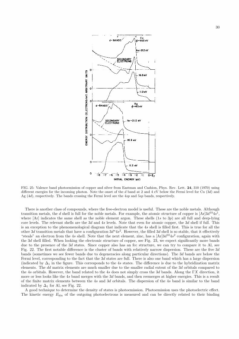
30
FIG. 25: Valence band photoemission of copper and silver from Eastman and Cashion, Phys. Rev. Lett. 24, 310 (1970) usingdifferent energies for the incoming photon. Note the onset of the d band at 2 and 4 eV below the Fermi level for Cu (3d) andAg (4d), respectively. The bands crossing the Fermi level are the 4sp and 5sp bands, respectively.
There is another class of compounds, where the free-electron model is useful. These are the noble metals. Althoughtransition metals, the d shell is full for the noble metals. For example, the atomic structure of copper is [Ar]3d104s1,where [Ar] indicates the same shell as the noble element argon. These shells (1s to 3p) are all full and deep-lyingcore levels. The relevant shells are the 3d and 4s levels. Note that even for atomic copper, the 3d shell if full. Thisis an exception to the phenomenological diagram that indicate that the 4s shell is filled first. This is true for all theother 3d transition metals that have a configuration 3dn4s2. However, the filled 3d shell is so stable, that it effectively“steals” an electron from the 4s shell. Note that the next element, zinc, has a [Ar]3d104s2 configuration, again withthe 3d shell filled. When looking the electronic structure of copper, see Fig. 23, we expect significantly more bandsdue to the presence of the 3d states. Since copper also has an fcc structure, we can try to compare it to Al, seeFig. 22. The first notable difference is the cluster of bands with relatively narrow dispersion. These are the five 3dbands (sometimes we see fewer bands due to degeneracies along particular directions). The 3d bands are below theFermi level, corresponding to the fact that the 3d states are full. There is also one band which has a large dispersion(indicated by ∆1 in the figure. This corresponds to the 4s states. The difference is due to the hybridization matrixelements. The dd matrix elements are much smaller due to the smaller radial extent of the 3d orbitals compared tothe 4s orbitals. However, the band related to the 4s does not simply cross the 3d bands. Along the ΓX direction, itmore or less looks like the 4s band merges with the 3d bands, and then reemerges at higher energies. This is a resultof the finite matrix elements between the 4s and 3d orbitals. The dispersion of the 4s band is similar to the bandindicated by ∆1 for Al, see Fig. 22.
A good technique to determine the density of states is photoemission. Photoemission uses the photoelectric effect.The kinetic energy Ekin of the outgoing photoelectrons is measured and can be directly related to their binding

31
energies Eb via
Ekin = ~ω −Eb, (102)
where ~ω (or hν) is the energy of the photon. The spectra for copper and silver are given in Fig. 25. Different photonenergies are used. The spectra look different due to changes in the matrix elements as a function of photon energy.What is clear is the strong emission from the d bands. The onset of is around 2 eV for copper and 4 eV for silver.The band width for copper is smaller than that of silver (this is most clearly seen in the spectra taken at 21.2 eV).This is in agreement with our notion that the 3d bands are smaller and therefore more localized than the 4d bands.The density of states at the Fermi level is rather small and due to the sp bands.
Another interesting effect occurs at the L point in the Brillouin zone. The Fermi surface lies just above the band atthe edge of the Brillouin zone. This situation is very similar to our example for the nearly-free electron model in twodimensions for n = 1.4 electrons per site, see Fig. 13 (in three dimensions, the ΓL direction is (111), whereas in twodimensions the (0, 0) (Γ in two dimensions) to (π
a ,πa ) direction is (1, 1). Note that the plot directions are opposite).
We saw that in two dimensions a neck was formed touching the edge of the Brillouin zone. A comparable effect occursin three dimension, see Fig. 24, where we find “neck” formation along the (111) directions.
XIV. OPTICAL SPECTROSCOPY
In a regular course on electricity and magnetism, the electronic structure is treated in a very approximate way (thissection will, unlike AM, follow SI units). The assumption is that an external electric field induces a polarization P
counteracting the external field. The external field is given by the displacement D which can be related to externalcharges that create the external field. The external field and the polarization together produce the electric field insidethe solid
E =1
ε0(D −P), (103)
where ε0 is the permittivity of free space (vacuum). We know from Gauss’s law that ∇ · E = ρ/ε0, where ρ is thecharge density. Taking the divergence of the above equation gives
ε0∇ ·E = ∇ · D −∇ · P ⇒ ρ = ρfree + ρind, (104)
where we have used ∇·D = ρfree and ∇·P = −ρind, giving the free and induced charges, respectively. The assumptionis now that the polarizability is directly proportional to the electric field
P = ε0χE, (105)
where χ is known as the electric susceptibility. This quantity is supposed to represent all the electronic structure ofthe solid. Often the solid is represented as a simple electron gas. Although this assumption works often surprisinglywell (it explains for example why light is reflected from metals, giving them the mirror-like appearance), it does notwork well when considering more details (for example, why is copper reddish, silver silver, and gold yellow). To obtainsome understanding about these details, we have to understand the interaction between light and solids in terms oftransitions in the electronic structure. However, let us first continue with the standard E&M approach.
Inserting Eqn. (105) into (103), gives
E =1
ε0(D − ε0χE) ⇒ E =
1
ε0(1 + χ)D =
D
ε0εr=
D
ε, (106)
where we have introduced the relative permittivity εr = 1 + χ, also known as the dielectric constant. We see thatonce we have found χ, we can also directly relate the electric field inside the solid to the externally applied field.
The Lorentz oscillator.− Let us first consider the example of a Lorentz oscillator. This classical model is useful sinceit can be related to quantum-mechanical interband transitions in a solid. We can also reduce it to the Drude modelwhich quantum mechanically includes all intraband transitions (i.e. no scattering with reciprocal lattice vectors).The quantum-mechanical theory can therefore be seen as an extension of its classical analog. We start by consideringNewton’s equation for an electron in an electric field
∑
F = ma ⇒ − eE−mΓv −mω20r = ma. (107)

32
Classically, this means that the electron feels an electric force −eE. It is held in its place by an effective spring force−mω2
0r from the nucleus. In addition, it feels a viscous damping −mΓv. Quantum mechanically, we will see that~ω0 corresponds to the energy of inter/intraband transtions. The damping is due to scattering giving a finite lifetime(and therefore a broadening Γ) to the electronic states. Eqn. (107) leads to a differential equation
d2r
dt2+ Γ
dr
dt+ ω2
0r = − e
mE. (108)
If the local electric field varies as e−iωt, then r e−iωt has a similar time dependence. Since r gives the displacementof the electron with respect to the nucleus, this gives an induced dipole moment
r = −eEm
1
ω20 − ω2 − iΓω
⇒ p = −er = α(ω)E with α(ω) =e2
m
1
ω20 − ω2 − iΓω
. (109)
The total polarization per unit volume is given by
P =N
Vp = nα(ω)E ≡ ε0χE ⇒ χ =
nα(ω)
ε0, (110)
where n = N/V is the electron density. This gives for the dielectric constant
εr = 1 + χ = 1 +nα(ω)
ε0= 1 +
ne2
mε0
1
ω20 − ω2 − iΓω
. (111)
We can reduce this to the Drude result by realizing that the Drude model excludes the attractive potential of thenuclei (ω0 = 0) and does not include scattering (Γ). This gives
εr = 1 − ne2
mε0
1
ω2= 1 −
ω2p
ω2, (112)
where ω2p = ne2/ε0m is the plasma frequency. This result basically has the electron gas moving along with the electric
field.Let us see what a typical value is for the plasma frequency. Let us consider aluminum. Al is face-centered cubic
with a lattice constant a = 4.05 A. Since this is fcc there are four atoms in the cube, see Fig. 20 (eight at thecorners that count for 1/8 and six at the sides that count for a 1/2). Al has a 3s23p configuration, so each Al atomcontributes three electrons. This gives a density n = 4 × 3/(4.05× 10−10)3 = 1.8 × 1029 m−3. Inserting the numbersgives ωp = 2.4 × 10¹⁶ s−1 or in energy ~ω = 99 eV. This is undoubtedly going to be too high since we know that theDrude model neglects the Fermi-Dirac statistics and therefore overestimates n.
Interaction of light with a solid.− This is all nice, but how does this affect the interaction of light with a solid, i.e.the optical properties of a solid? Let us go back to Maxwell equations. Two of them include the divergence of theelectric and magnetic fields
∇ · D = ρfree → ∇ · (εRE) = ρfree = 0, (113)
in the absence of an applied electric field. Some care should be taken here with the permittivity. We use here a realpermittivity εR = Re[ε]. As we will see the complex part will be related to the currents. Furthermore, we also havefor the magnetic induction ∇ ·B = 0. The other two involve the rotation of the magnetic and electric fields.
∇×E +∂B
∂t= 0 and ∇×H− ∂D
∂t= Jfree, (114)
where Jfree is the current due to the free charges. Since we are interested in the propagation of a wave in a solid, wewant to transform these equations into a wave equation. This can be done by taking the rotation as follows
∇×∇×E = ∇(∇ ·E) −∇2E = −∇× ∂B
∂t. (115)
In an isotropic medium, we have the relation B = µH (similar to the relation D = εE). Since ∇ · E = 0, we obtainwith the use of the other Maxwell equation
∇2E = µ∇× ∂H
∂t= µ
∂
∂t(∇×H) = εRµ
∂2E
∂t2+ µ
∂Jfree
∂t. (116)

33
For the current, we have apply Ohm’s law: J = σE, where σ is the conductivity. This gives us the wave equation
∇2E− εRµ∂2E
∂t2= µσ
∂E
∂t. (117)
The term with σ is related to the optical conductivity related to optical transitions accompanying photon absorption.Remember that the wave equation in free space is given by
∇2E− ε0µ0∂2E
∂t2= 0, (118)
where ε0µ0 = 1/c2, where c is the speed of light in vacuum. We will now look for solution of the electric field in asolid of the form
E = E0eiq·r−iωt. (119)
Inserting into Eqn. (116) gives
−q2 + εRµω2 = −iµσω ⇒ q2 =
µrε1c2
ω2 + iµrµ0σω = µrω2
c2
(
ε1 + ic2µ0σ
ω
)
= µrω2
c2
(
ε1 + iσ
ε0ω
)
, (120)
where εR ≡ ε0ε1 and µr = 1 in a nonmagnetic solid. We can only find a solution if the wavevector is complex, whichmeans we allow for evanescent waves. Let us define a complex diffractive index n,
q =ω
cn =
ω
c(n+ iκ), (121)
where n is the refractive index and κ is the extinction coefficient (many books use k or K here, but this notation is abit confusing). Substituting gives
ω2
c2(n+ iκ)2 =
ω2
c2(n2 − κ2 + 2inκ) ≡ µr
ω2
c2
(
ε1 + iσ
ε0ω
)
, (122)
or
ε1 =n2 − κ2
µrand
σ
ε0ω=
2nκ
µr. (123)
Often this is written as a complex dielectric function
εr = ε1 + iε2 =n2
µr, (124)
giving
ε1 = ε =n2 − κ2
µrand ε2 =
σ
ε0ω=
2nκ
µr. (125)
Let us consider nonmagnetic systems from now on, for which we have
ε1 = ε = n2 − κ2 and ε2 = 2nκ. (126)
We can also invert these equations to find the expressions for n and κ in terms of ε1 and ε2. Writing
n2 −( ε2
2n
)2
− ε1 = 0 ⇒ n4 − ε1n2 −
(ε22
)2
= 0 (127)
This is a cubic equation in n2, where the roots are given by
n2 =1
2ε1 +
1
2
√
ε21 + 4(ε2
2
)2
, (128)
or
n =
√
1
2ε1 +
1
2
√
ε21 + ε22. (129)

34
Ei
Hi
Er
Hr
FIG. 26: The reflectance of light at the surface of a solid.
Similarly, we can find
κ =
√
−1
2ε1 +
1
2
√
ε21 + ε22. (130)
We can split the dielectric constant that we obtained before into a real and imaginary part
εr = 1 +ne2
mε0
1
ω20 − ω2 − iΓω
. = 1 +ne2
mε0
ω20 − ω2
(ω20 − ω2)2 + Γ2ω2
+ ine2
mε0
Γω
(ω20 − ω2)2 + Γ2ω2
. (131)
which gives
ε1 = 1 +ne2
mε0
ω20 − ω2
(ω20 − ω2)2 + Γ2ω2
and ε2 =ne2
mε0
Γω
(ω20 − ω2)2 + Γ2ω2
. (132)
As we will see later on, ε2 is related to the absorption. Note that the function is like a Lorentzian (it is plotted inFig. 32), with a width related to Γ. Note that in the limit Γ → 0 this function becomes a δ-function, going to zerofor ω 6= ω0 and having a value of 1/ωΓ → ∞ for ω = ω0. This means that the solid can only absorb light with energy~ω0. Obviously, few solids have only one resonance frequency. However, we can easily generalize the Lorentz oscillatorproblem for many oscillators. Let us take nj the density of electrons bound with resonance frequency ωj
εr = 1 +∑
j
nje2
mε0
1
ω2j − ω2 − iΓjω
, (133)
with∑
j nj = n.
Drude model and intraband transitions.− Although the Drude model fails in a quantitative description of a solid (bygrossly overestimating the number of electrons relevant for the conductivity and other properties, due to the neglectof Fermi-Dirac statistics), the idea that the conduction is determined by electrons that behave almost freely worksrather well. This implies that ω0 = 0 The value of Γ is can be related to the inverse of the mean free time betweencollisions, Γ = 1/τ . This gives for the dielectric functions
ε = 1 −ω2
pτ
ω(ωτ + i)⇒ ε1 = 1 −
ω2pτ
2
1 + ω2τ2and ε2 =
ω2pτ
ω(1 + ω2τ2)(134)
Reflectance.− Although there are many different types of optical spectroscopies, one of the most intuitive ones isthe reflectance. Let us consider an wave coming in perpendicular, see Fig. 26. Let us take the incident electric fieldalong the x-direction,
Ei = Eieiqz−iωtx, (135)
where q can be complex. We can find the magnetic field from the Maxwell equation
∇×E = −µ∂H∂t
= iµωH. (136)

35
−20
−15
−10
−5
0
5
10
0 0.5 1 1.5 2ω/ω
p
ε 1,ε2
ε1
ε2
FIG. 27: The dependence of ε1 and ε2 as a function of ω (normalized to the plasma frequency ωp) of the Drude model. Thescattering is small, i.e. Γ = τ−1 � ωp.
The rotation can be obtained from
∇×E =
∣
∣
∣
∣
∣
∣
x y z∂∂x
∂∂y
∂∂z
Ex 0 0
∣
∣
∣
∣
∣
∣
=∂Ex
∂zy = iqExy (137)
This gives
Hi =q
µωEie
iqz−iωty, (138)
which means H is perpendicular to E (as it should be). At the surface part of the wave is reflected and part of it istransmitted. However, the other Maxwell equations impose continuity of the electric field
Ei +Er = Et, (139)
where r and t stand for reflected and transmitted, respectively. For the magnetic field, we must satisfy
Hi −Hr = Ht, (140)
where we should take care the the direction of the magnetic field changes for the reflected light, see Fig. 26. We canrelate this to the electric field by
q1µ1ω
(Ei −Er) =q2µ2ω
Et, (141)
Using that q = ωn/c and that medium 1 is the vacuum for which we have n1 = 1 and µ1 = µ0 and, in addition,taking the solid nonmagnetic, which gives µ2 = µ0, we obtain
Ei −Er = nEt. (142)

36
0
0.5
1
1.5
2
2.5
3
3.5
4
0 0.5 1 1.5 2ω/ω
p
n,κ
κ
nn
TransparentReflecting
FIG. 28: The dependence of n and κ as a function of ω (normalized to the plasma frequency ωp) for the Drude model. SameΓ as in Fig. 27.
0
0.2
0.4
0.6
0.8
1
0 0.5 1 1.5 2 2.5
R
ω/ωp
FIG. 29: The dependence of the reflectivity R as a function of ω (normalized to the plasma frequency ωp) for the Drude model.Same Γ as in Fig. 27.
Combining this with Eqn. (139) gives
(n− 1)Ei + (1 + n)Er = 0 ⇒ r =Er
Ei=
1 − n
1 + n. (143)
The reflectivity is then given by
R = r∗r =
∣
∣
∣
∣
1 − n
1 + n
∣
∣
∣
∣
2
=(1 − n)2 + κ2
(1 + n)2 + κ2(144)

37
FIG. 30: The reflectance of aluminum. The plasma frequency is given by ~ωp = 14.7 eV. The decrease in reflectance around1.4 eV is due to a weak interband transition.
Given the expressions for ε1 and ε2, see Fig. 27, for the Drude model, it is straightforward to calculate the indexof refraction n = n + iκ and the reflectivity, see Fig. 28 and 29. Let us first look at the most intuitive one: thereflectivity, see Fig. 29. In the Drude, we see that the reflectivity is close 100% up to the plasma frequency ωp. Howdoes this work out for our “prototype” nearly-free electron system Al? Figure 30 shows that there is a remarkableagreement in the reflectivity. Close to 90% of the light is reflected up to the plasma frequency. The wavelength ofvisible light ranges from 380 (violet) to 750 (red) nm. This corresponds to an energy of 1.66-3.27 eV. The value of~ωp for Al is 14.7 eV. Therefore all the visible light is reflected, explaining why aluminum foil has the mirror-like look.The difference in the two sides of the aluminum foil has to do with the manufacturing process. Since aluminum foilis so thin, two sheet of foil are placed on top of each other in the final rolling. When separated after rolling the insideis duller than the outside due to different surface roughness. The reflectance is 88% for the shiny side and 80% forthe dull side. There is a decrease in reflectance deviating from the Drude-like behavior around 1.4 eV due to weakinterband transitions. The plasma frequency is ωp = 3.5 s−1. This corresponds to a density of n = 3.9 × 1027 m−3.So when neglecting the Fermi-Dirac distribution, we overestimate n by a factor 50. (As you might remember from566, two order of magnitude was roughly the overestimation of the conductivity in the Drude model, which is givenby σ = ne2τ/m, where τ is the time between scattering events. However, even though the model completely missesthe actual value of ωp, it gives a very nice description of the reflectivity.
The reflectance for frequencies less than the plasma frequency also manifests itself in other quantities. For ω < ωp,the extinction coefficient is finite, indicating that light does not penetrate the solid. For ω > ωp we obtain no extinctionand obtain a finite index of refraction. Thus aluminum will become transparent in the ultraviolet. We also observe a

38
k
EE
FDrude like excitations
Lorentz like excitations
"localized" bands
"free-electron" bands
FIG. 31: Schematic figure of the possible transitions. The Drude model describes intraband transition. For free electron likesystems and noble metals that would be in the free electron like bands that cross the Fermi level. The minimum energy neededfor these transitions is zero. However, for noble metals, one also has to consider interband transitions from the more localized3d bands. These occur at a finite energy.
finite refractive index n close to ω = 0. This is due to absorption related to the fact that ω0 = 0 for the Drude model.Lorentz oscillators and interband transitions.−
However, the Drude model appears to fail for noble metals, such as copper (reddish) and gold (yellow), althoughit works reasonably well for silver. The electron density of copper is n = 4 × 1/(3.61 × 10−10)3 = 8.5 × 1028 m−3.This about a factor two smaller than that of aluminum (although the absolute densities fail to predict the plasmafrequency, your first order guess for the ratio of the plasma frequencies would be the ratio of the electron densities).
Naively one can expect the plasma frequency to be about a factor√
2 smaller. This would be of the order of 10eV, sufficiently high to reflect all visible light. However, to obtain absorption in the visible light we need a plasmafrequency around 2 eV, about seven times smaller. Since ωp ∼ √
n, this would correspond to an electron densitywhich is about a factor 50 smaller. Although we might be willing to swallow a factor two, this is a bit too much.To understand the difference one needs to take a closer look at the electronic structure. The Drude model describesintraband transition. For free electron like systems like aluminum, these occur in the bands that cross the Fermilevel. The minimum energy needed for these transitions is zero. However, for noble metals, one also has to considerinterband transitions from the more localized d bands. These occur at a finite energy.
Let us therefore return to the original expressions for ε, see Eqn. (111). The real and imaginary part of the dielectricfunction, ε1 and ε2 are plotted in Fig. 32. The refractive index n, extinction coefficient κ, and the reflectivity R areshown in Fig. 33 for ω0 = ωp/2. Again, let us first look at the reflectivity. In the limit that Γ → 0, we see again thata decrease in reflectivity around ωp. This transition occurs when ε1 = 0, or, for Γ = 0,
ε1 = 1 +ω2
p
ω20 − ω2
= 0 ⇒ ω =√
ωp + ω20 . (145)
This gives or our example ωp
√
1 +(
12
)2 ∼= 1.12 ωp. Above this energy, the solid is transparent. Below this energy the
solid is reflecting down to the energy ω0. Below that energy, the system becomes transparent again. This situation isvery comparable to what is found for semiconductors or insulators. For a wide-band insulator (for example, diamond,see Fig. 34) an optical transition occurs at a finite energy, i.e. the energy needed to excite an electron from the valenceband into the conduction band. Below that energy, the system becomes transparent. For diamond, the minimumexcitation energy is greater than 5 eV, larger than the energy of visible light. This makes diamond transparent forvisible light giving it a glass light appearance. However, the reflectance is not entirely zero and some of the light willtherefore be reflected. Diamonds can also have a color. This is due to impurities. These impurities create energystates inside the insulating gap. In Fig. 33, the optical properties are divided into four regions. These regions roughlyindicate the dominant aspect of the material. For ω less than roughly 0.4ω0, the material is mainly transparent with

39
-10
-5
0
5
10
15
20
0 0.5 1 1.5 2
ε 1,ε2
ω/ωp
ε2
ε1
FIG. 32: The coefficients ε1 and ε2 as a function of ω/ωp with ω0 = ωp/2 and Γ = 0.1ωp.
0
0.5
1
1.5
2
2.5
3
3.5
4
0 0.5 1 1.5 2
R,n
,κ
ω/ωp
R
κ
n
ReflectingTransparent
Absorbing
Transparent
R for Γ∼0
FIG. 33: The refractive index n, extinction coefficient κ, and the reflection coefficient R for a Lorentz oscillator as a functionof ω/ωp with ω0 = ωp/2 and Γ = 0.1ωp.
a finite refractive index n and a small extinction coefficient κ. Around ω0, the material is predominantly absorbing,where the incoming light causes transitions of energy ~ω. Between 0.6~ω0 and ωp, the system is reflecting with alarge R. For energies greater than ωp, we again observe transparent behavior.
When considering the reflectance of noble metal such as copper and silver, see Fig. 35, one has to consider acombination of both Drude and Lorentz excitations. The Drude excitations related to excitations in the 4sp bandscrossing the Fermi level dominate the reflectance for low energies. However at approximately 2 and 4 eV for Cu andAg, respectively, we observe Lorentz-like excitations related to transitions from the occupied 3d band into the empty4sp states, see also Fig. 25. To describe the reflectance we cannot consider a single Lorentz oscillator, but we have totake into account a large number of Lorentz oscillators of different energy. This causes a sharp drop in reflectance.For Ag, this hardly affects the reflectance in the visible light, since 4 eV is in the ultraviolet. However, for copper, thedecrease in reflectance occur in the visible region, cutting of the blue part of the spectrum, giving copper its reddish

40
FIG. 34: The band structure of diamond after Saslow, Bergstresser, and Cohen, Phys. Rev. Lett. 16, 354 (1966). The insetshows the values of several optical transitions.
color. Note that another drop of occurs at higher energies, clearly visible in Ag around 7-8 eV. This drop-off is relatedto the plasma frequency at an energy about half that in Al, in agreement with our simple estimate of the relativeplasma frequencies of Al and Ag/Cu.
XV. QUANTUM-MECHANICAL TREATMENT OF OPTICAL SPECTROSCOPY
We now want to interpret optical spectroscopy in term of quantum mechanics and relate the Lorentz oscillators tointerband and intraband transitions. We can write our eigenstates in the absence of light as
H0 = |kn〉 = Ekn|kn〉, (146)
where H0 is the Hamiltonian describing the solid and Ekn are the eigenenergies that describe the electronic structure.We want to study how the solid reacts to light and we therefore add a time-dependent perturbation to the Hamiltonian,
H = H0 +H ′(t). (147)
The wave function as a function of time can now be found from the time-dependent Schrodinger equation
i~∂
∂t|ψ(t)〉 = [H0 +H ′(t)]|ψ(t)〉. (148)
The question is now, what states are involved in the wavefunction |ψ(t)〉? We have to make some approximationshere. Obviously, we want to include the ground state, which is the Fermi sea, i.e. all the states filled up to the Fermilevel following Pauli’s principle (we assume that T = 0 K). For the Fermi sea, which we denote by |0〉, we have
H0|0〉 = E0|0〉 with E0 =∑
Ekn≤EF
Ekn. (149)
Let us now consider the excited states. To lowest order, the light will create electron-hole pair excitations with respectto the Fermi sea. Let us denote these states by
|m〉 = |k′n′;kn〉 (150)

41
FIG. 35: The reflectance of copper and silver, see Ehrenreich and Philipp, Phys. Rev. 128, 1622 (1962).
where the state |k′n′;kn〉 indicates a Fermi sea, but with an electron with wave vector k′ and band index n′ above theFermi level and a hole (or missing electron) with wavevector k and band index n below the Fermi level. The energyof this state is given by
H0|m〉 = Em|m〉 = (~ωm +E0)|m〉 with ~ωm = Ek′n′ −Ekn. (151)
We can now write the time-dependent wavefunction as
|ψ(t)〉 =∑
m
am(t)e−iEmt/~|m〉. (152)
Inserting this into the Schrodinger equation gives
i~∑
m
{
dam(t)
dt− i
~Ema(t)
}
e−iEmt/~|m〉 =∑
m
{Em +H ′(t)} am(t)e−iEmt/~|m〉. (153)
We see that the terms with Em cancel, giving
i~∑
m
dam(t)
dte−iEmt/~|m〉 =
∑
m
H ′(t)am(t)e−iEmt/~|m〉. (154)
We can multiply this on the left by 〈m′|eiEmt/~, giving
i~dam′(t)
dt=∑
m
〈m′|H ′(t)|m〉am(t)ei(Em′−Em)t/~. (155)

42
If we take the system to be initially in the ground state,
am = δm,0, t = 0, (156)
we obtain Em′ −Em = Em′ −E0 = ~ωm. Using
H ′m′ = 〈m′|H ′(t)|0〉 =
∫
drϕ∗k′n′H ′ϕkn, (157)
we can write, in first order approximation theory,
i~dam′(t)
dt= H ′
m′eiωm′ t. (158)
Note that the summation has disappeared since we only consider one transition, from the ground state |0〉 to andexcited state |m′〉.
So far we have not really specified the pertubation H ′(t). For a classical oscillator, we can write
H ′(t) = eE(t) · r. (159)
We are concerned with the situation that the wavelength of the light is much larger than the dimension of the atom.So we can therefore approximate the electric field by its value at the nucleus. Let us consider monochromatic lightwith a cosine dependence (we can always express other light in these components),
E(t) = E cosωt =1
2E(eiωt + e−iωt). (160)
We can then express
H(t) =1
2eE · r(eiωt + e−iωt) ⇒ H ′
m =1
2eE · 〈r〉m(eiωt + e−iωt), (161)
where
〈r〉m = 〈m|r|0〉 =
∫
drϕk′n′rϕkn (162)
is the dipole matrix element, which follows the usual dipole selection rules Let us drop the prime in Eqn. (158) andintegrate the time from t = 0 to a particular time t
am(t) =1
i~
1
2eE · 〈r〉m
∫ t
0
dt′[
ei(ωm+ω)t′ + ei(ωm−ω)t′]
(163)
=eE · 〈r〉m
2~
[
1 − ei(ωm+ω)t
ωm + ω+
1 − ei(ωm−ω)t
ωm − ω
]
. (164)
We are interested in comparing the classical with the quantum-mechanical dielectric function. We obtained theclassical dielectric function by studying the induced dipole moment due to the electric field. Let us consider calculatethe induced dipole moment which can be directly related to the expectation value of r,
p = −e〈ψ(t)|r|ψ(t)〉. (165)
However, we just obtained the expression for |ψ(t)〉 within first-order perturbation theory. Using this, we have
p = −e∑
m,m′
a∗m′(t)am(t)〈m′|r|m〉ei(Em′−Em)t/~. (166)
However, we expect that the coefficients am with m 6= 0 are relatively small. Therefore, the major contributions willcome from the terms where either m = 0 or m′ = 0. Renaming one of the dummy arguments gives
p = −e∑
m
[
a∗m(t)〈m|r|0〉eiωmt + am(t)〈0|r|m〉e−iωmt]
= −e∑
m
[
a∗m(t)〈r〉meiωmt + am(t)〈r〉∗me−iωmt]
(167)

43
Let us now also assume that the excited states have a finite lifetime. This means that they obtain a complex frequency
ωm → zm = ωm +i
2Γm, (168)
giving a time dependence eiωt− 12Γmt, showing a decay of the wavefunction. In the remainder, we neglect the m
dependende of Γ. We are now dealing with terms
am(t)e−izmt =eE · 〈r〉m
2~
[
e−izmt − eiωt
zm + ω+e−izmt − e−iωt
zm − ω
]
→ −eE · 〈r〉m2~
[
eiωt
zm + ω+
e−iωt
zm − ω
]
, (169)
where in the last step we have used the fact that only the terms with the same frequency as the driving force remainwhn taking a time average. Let us for simplicity also take the electric field along the x direction, with E = E x. Thisgives also a dipole moment px along the x direction. Using xm = 〈m|x|0〉, we find for the dipole moment
p =∑
m
e2E|xm|22~
(zm + z∗m)
[
eiωt
(zm + ω)(z∗m − ω)+
e−iωt
(zm − ω)(z∗m + ω)
]
, (170)
where zm + z∗m = 2ωm and
(zm ± ω)(z∗m ∓ ω) = (ωm +i
2Γ ± ω)(ωm − i
2Γ ∓ ω) (171)
= (ωm ± ω)(ωm ∓ ω) +i
2Γ[ωm ∓ ω − (ωm ± ω)] − 1
4Γ2 (172)
= ω2m − ω2 − 1
4Γ2 ∓ iΓω → ω2
m − ω2 ∓ iΓω, (173)
where in the last step we assumed that the broadening is small relatively to the excitation energy ωm. This gives forthe dipole moment
p =∑
m
e2E|xm|2~
[
ωmeiωt
ω2m − ω2 − iΓω
+ωme
−iωt
ω2m − ω2 + iΓω
]
. (174)
The polarization is then given by
P =N
Vp =
∑
m
2e2n|xm|2~
[
ωm(ω2m − ω2)
(ω2m − ω2)2 + Γ2ω2
cosωt+ωmΓω
(ω2m − ω2)2 + Γ2ω2
sinωt
]
E. (175)
In order to relate this to the dielectric function, we need to look at the response to a cosine wave. We know thatfor an electric field E e−iωt, the polarization is given by P = χ(ω)ε0E. To construct a cosine, we also need χ(−ω).From Eqn. (111), we can see that replacing ω by −ω gives ε(−ω) = ε∗(−ω). We therefore have for a cosine
P =1
2ε0E(χe−iωt + χ∗eiωt) =
1
2ε0E
[
(ε1 − 1)(e−iωt + eiωt) + iε2(e−iωt − e+iωt)
]
(176)
= ε0(ε1 − 1)E cosωt+ ε0ε2E sinωt. (177)
This means that the cosine term is related to ε1,
ε1 = 1 +∑
m
2e2n|xm|2ε0~
ωm(ω2m − ω2)
(ω2m − ω2)2 + Γ2ω2
(178)
and the sine term to ε2,
ε2 =∑
m
2e2n|xm|2ε0~
ωmΓω
(ω2m − ω2)2 + Γ2ω2
. (179)
We can also write this in its complex form
εr = 1 +ne2
mε0
∑
m
fm
ω2m − ω2 − iΓω
, (180)
with the oscillator strength given by
fm = ~ωm2m
~2|xm|2. (181)

44
XVI. RELATION TO ABSORPTION
Earlier it was mentioned that ε2 was related to absoprtion. This might not be directly obvious. We are used torighting absorption and emission in terms of Fermi’s Golden Rule
I(ω) ∼∑
m
|〈m|H ′|0〉|2δ(ω − ωm), (182)
where I(ω) is the absorption intensity. However, we want rewrite the δ-function. Using
−i∫ ∞
0
ei(ω−ωm)t−ηtdt =1
ω − ωm + iη=
ω − ωm
(ω − ωm)2 + η2− i
η
(ω − ωm)2 + η2(183)
Note that the imaginary part works as a δ-function in the limit η → 0, when it is zero for ω 6= ωm and 1/η → ∞ forω = ωm. The integral over this function, known as a Lorentzian, is equal to π. Normalizing the δ-function to unity,we have
δ(ω − ωm) =1
π
η
(ω − ωm)2 + η2= − 1
πIm
1
ω − ωm + iη. (184)
The function (ω−ωm + iη)−1 is also known as a Green’s function. Therefore we can also write Fermi’s golden fule as
I(ω) ∼ − 1
π
∑
m
|xm|2Im 1
ω − ωm + iη= − 1
π
∑
m
|xm|2Im 1
ω − z∗m, (185)
where we have used xm = 〈m|H ′|0〉. We can also do the inverse process and emit a photon
I(ω) ∼∑
m
|〈0|H ′|m〉|2δ(ωm + ω). (186)
This term requires some closer consideration. The conservation of energy says that we start we an initial state andend up with an excitation with energy ~ωm and a photon with energy ~ω. Since energy is conserved this implies that~ω = −~ωm. Since the photon energy is always positive, this implies that ~ωm < 0. However,we saw before that the~ωm corresponded to an electron-hole pair excitation, which is always positive. However, we can have this term ifthere are excitations in the initial state, which can be present at finite temperature or due to laser excitations. Thenthe energy ~ωm corresponds to the deexcitation of an electron-hole pair. We can also rewrite this in an integral form
i
∫ 0
−∞ei(ωm+ω)t+ηtdt = − 1
ωm + ω + iη= − 1
ω + zm(187)
The gives for the intensity
I(ω) ∼ − 1
π
∑
m
|xm|2Im 1
ω + zm, (188)
Adding the two terms together gives
1
ω − z∗m− 1
zm + ω= − zm + z∗m
(ω − z∗m)(ω + zm), (189)
which reproduces the eiωt term in Eqn. (173).
XVII. THOMAS-FERMI SCREENING
As we have seen in the previous sections, the electrons respond to an externally applied electric field. In the sameway, one can envision the electron cloud corresponding to the electric field produced by an electron. This is calledscreening. We can understand screening physically by noting that the electrons cloud reacts to the electron and willmove as a result of the potential created by the electron. However, in a system in equilibrium we assume that the
45
chemical potential µ = EF (r) − U(r) remains constant. Thus the change in potential has to be compensated by achange in number of electrons
dEF
dn∆n− U = 0. (190)
In a free electron model, the Fermi energy is given by
N = 2V
(2π)34
3πk3
F ⇒ kF = (3π2n)1/3 ⇒ EF =~
2k2F
2m=
~2
2m(3πn)2/3, (191)
giving dEF /dn = 23EF /n. The induced charge is therefore
ρind = e∆n =3
2
enU
EF=
3
2
e3n
EF ε0q2(192)
where use has been made of Laplace’s equation to calculate the potential from the point charge e: ∇2V = e/ε0(which also follows from Gauss’s equation ∇ · E = −e/ε0 and E = −∇V . or in momentum space −q2V = e/ε0 orV = −e/ε0q2. The potential energy is then U = −eV = e2/ε0q
2. An alternative way of obtaining the same result isto make a Fourier transform of the Coulomb potential
U(r) =1
4πε0
e2
r. (193)
The use of this alernative way becomes clear in a little while. The Fourier transform gives
Uq =e2
4πε0
∫ 2π
0
dϕ
∫ ∞
0
dr
∫ π
0
dθr2 sin θeiqr cos θ 1
r(194)
=e2
2ε0
∫ ∞
0
dr
∫ 1
−1
d cos θreiqr cos θ =e2
2iqε0
∫ ∞
0
dr(eiqr − e−iqr) (195)
Here we have a small problem with the convergence of the integration. This can be solved by making the oscillationdamp out by e−λr, and in the end take λ = 0
Uq =e2
2iqε0
∫ ∞
0
dr(eiqr − e−iqr)e−λr =e2
2iqε0
∫ ∞
0
dr(ei(q+iλ)r − e−i(q−iλ)r) =e2
2qε0
[
1
q + iλ+
1
q − iλ
]
=e2
ε0
1
q2 + λ2(196)
where a λ has been introduced to let the oscillations damp out slowly. In the limit λ→ 0, we obtain Uq = e2/ε0q2.
For the dielectric function we then find
εr = 1 + χ = 1 − ρind
ρfree= 1 − ρind
−e = 1 +3e2n
2EF ε0q2= 1 +
q2TF
q2(197)
with qTF =√
3ne2/2ε0EF . We therefore find an effective Coulomb potential
Uq =1
ε
e2
q2=
1
ε+ 0
e2
εrq2=
1
4πε0
e2
q2 + q2TF
. (198)
One might wonder to what potential this corresponds in real space. However, we see that the form is exactly the sameas the form obtained in deriving the Fourier transform of the potential. We can therefore write the effective screenedpotential as
U(r) =1
4πε0
e2
re−qF r, (199)
which look like a Coulomb potential but with a reduced range.

46
XVIII. MANY-PARTICLE WAVEFUNCTIONS
In quantum mechanics, particles are indistinguishable. This means that we should be able to interchange twoparticles without seeing any effect on the probability function. We can distinguish two fundamentally different typesof particles, namely those with a symmetric and antisymmetric wavefunction. Under permutation between particle iand j for a N particle wavefunction, one has the following possibilities
Pijψ±n1···nN
(r1, · · · , ri, · · · , rj , · · · , rN ) = ±ψ±n1···nN
(r1, · · · , ri, · · · , rj , · · · , rN ) (200)
where ki means that a particle is in a certain quantum state ni (for example a particle in a box where the quantumnumbers are ni = nx, ny, nz, but it could also refer to the quantum numbers of an atom ni = nlmσ). At first sightone might think it does not make any difference since the real properties are related to the square of the wavefunctionand a plus or minus sign should not make too much of a difference. However, the sign has drastic consequences forthe statistics. Let us look at the wavefunction for two particles:
ψ±k1,k2
(r1, r2) =1√2(ϕk1
(r1)ϕk2(r2) ± ϕk2
(r1)ϕk1(r2)). (201)
where φk are eigenfunctions of the Hamiltonian. The symmetric and antisymmetric wavefunctions give two fun-damentally different particles. Particles whose wavefunction is symmetric are bosons, particles with antisymmetricwavefunctions are called fermions. Examples of bosons are photons, π and K mesons. These are particles withintegral spin. Also the harmonic oscillator and lattice vibrations (also known as phonons) behave like a “boson”-likeparticle. Particles with half integral spin behave like fermions. Examples are electrons, protons, and neutrons. Theantisymmetric wavefunctions have a very special characteristic. Let us take two particle in the same quantum state
ψ−k,k(r1, r2) =
1√2(ϕk(r1)ϕk(r2) − ϕk(r1)ϕk(r2)) = 0. (202)
Therefore, it is impossible to have two fermions with the same quantum numbers. Note that the spin is also considereda quantum number. Therefore, we can have two electrons in the same wavefunction (say the same plane wave or thesame atomic orbital), but with opposite spins. The occupation of each fermion state is therefore 0 or 1.
Let us now generalize the wavefunctions for an arbitrary number of particles. For bosons the general wavefunctionis
Ψk1,...,kN=
√
Πinki!
N !
∑
P
ψk1(r1) · · ·ψkN
(rN ), (203)
where the summations runs over all the possible permutations of different indices ki. This gives the normalizationconstant. nki
indicates how many k-values are ki. Note that the∑
i nki= N . For two particles with S = 0, we have
Ψk1,k2=
1√2{ψk1
(r1)ψk2(r2) + ψk2
(r1)ψk1(r2)} . (204)
For k1 = k2 = k, we find
Ψk1,k2=
√
2!
2!ψk(r1)ψk(r2) = ψk(r1)ψk(r2), (205)
using the fact that nk = 2. We see that it is possible to put two bosons in the same quantum state. In fact, we canput any arbitrary number of bosons in a particle quantum state. From a statistical point of view, we therefore havefor the occupation numbers of a particular quantum state i
ni = 0, 1 fermions (206)
ni = 0, 1, 2, 3, · · · bosons (207)
This is an important aspect that we have to include in our quantum statistics. Up till now the only aspect that wehave used is the indistinguishability.
The situation for electrons (and other spin-1/2 particles) is fact a bit more complicated since the total wavefunction,i.e., orbital and spin, has to be asymmetric. This means ψS(r1, r2)ξA(1, 2) or ψA(r1, r2)ξS(1, 2), where ξ(1, 2) is thewavefunction for the spin. There are four ways to combine two spins ξ↑(1)ξ↑(2), ξ↑(1)ξ↓(2), ξ↓(1)ξ↑(2), and ξ↓(1)ξ↓(2).
47
ξ↑(1)ξ↑(2) and ξ↓(1)ξ↓(2) are clearly symmetric spin functions, since interchange of the particles does not change thesign of the wave function. These are the ξ11(1, 2) and ξ1,−1(1, 2) components of the triplet (S = 1). Since Sz = 1, 0,−1for S = 1, there should also be a S = 0 component. This can be obtained by using the step operator for the spin
S−ξ11 =√
(1 + 1)(1 − 1 + 1)ξ10 =√
2ξ10 = ξ↑(1)ξ↓(2) + ξ↓(1)ξ↑(2) (208)
⇒ ξ10 =1√2
[ξ↑(1)ξ↓(2) + ξ↓(1)ξ↑(2)] (209)
where we have used
S±ξSSz=√
(S ∓ Sz)(S ± Sz + 1)ξS,Sz±1 (210)
Note that this is also a symmetric wavefunction. The remaining wave function has to be orthogonal to the previousone
ξ00(1, 2) =1√2
[ξ↑(1)ξ↓(2) − ξ↓(1)ξ↑(2)] (211)
which is antisymmetric. Since there is only one component (called a singlet), this has to be S = 0. The four totalwavefunctions for two electrons are therefore Ψ1Sz
(r1, r2) = ψA(r1, r2)ξ1Sz(1, 2) with Sz = 1, 0,−1 and Ψ00(r1, r2) =
ψS(r1, r2)ξ00(1, 2). The S = 1 and Sz = 1 is given by
Ψ11(r1, r2) = ψA(r1, r2)ξ11(1, 2) =1√2
[ϕk1(r1)ϕk2
(r2) − ϕk2(r1)ϕk2
(r1)] ξ↑(1)ξ↑(2) (212)
=1√2
[ϕk1(r1)ξ↑(1)ϕk2
(r2)ξ↑(2) − ϕk2(r1)ξ↑(1)ϕk2
(r1)ξ↑(2)] (213)
=1√2
∣
∣
∣
∣
ϕk1(r1)ξ↑(1) ϕk1
(r2)ξ↑(2)ϕk2
(r1)ξ↑(1) ϕk2(r2)ξ↑(2)
∣
∣
∣
∣
(214)
The S = 0 and Sz = 0 wavefunction is given by
Ψ00(r1, r2) = ψS(r1, r2)ξ00(1, 2) =1√2
[ϕk1(r1)ϕk2
(r2) + ϕk2(r1)ϕk2
(r1)]1√2
[ξ↑(1)ξ↓(2) − ξ↓(1)ξ↑(2)] (215)
=1
2[ϕk1
(r1)ξ↑(1)ϕk2(r2)ξ↓(2) − ϕk2
(r1)ξ↓(1)ϕk1(r2)ξ↑(2) (216)
−ϕk1(r1)ξ↓(1)ϕk2
(r2)ξ↑(2) + ϕk2(r1)ξ↑(1)ϕk1
(r2)ξ↓(2)] (217)
Note that this can also be written as a combination of Slater determinants
Ψ00(r1, r2) =1√2
(
1√2
∣
∣
∣
∣
ϕk1(r1)ξ↑(1) ϕk1
(r2)ξ↑(2)ϕk2
(r1)ξ↓(1) ϕk2(r2)ξ↓(2)
∣
∣
∣
∣
− 1√2
∣
∣
∣
∣
ϕk1(r1)ξ↓(1) ϕk1
(r2)ξ↓(2)ϕk2
(r1)ξ↑(1) ϕk2(r2)ξ↑(2)
∣
∣
∣
∣
)
(218)
=1√2[ψk1↑,k2↓(r1, r2) − ψk1↓,k2↑(r1, r2)] (219)
Note that in general we can built up antisymmetric states from Slater determinants
ψk1σ1,...,kN σN(r1 · · · rN ) =
1√N !
∣
∣
∣
∣
∣
∣
∣
ϕk1(r1)ξσ1
(1) · · · ϕk1(rN )ξσ1
(N). .. .
ϕkN(r1)ξσN
(1) · · · ϕkN(rN )ξσN
(N)
∣
∣
∣
∣
∣
∣
∣
(220)
where σi =↑, ↓. As a result of the properties of the determinant, having two columns with the same k and σ impliesthat the determinant is zero, just as for the exclusion principle. Interchange of two columns also leads to a change insign of the determinant, giving us directly the antisymmetry. This is obvious for the Sz = 1,−1 states of the triplet.For the Sz = 0 states, one needs a combination of Slater determinants
Ψk1k2,00 =1√2
(ψk1↑,k2↓ − ψk1↓,k2↑) and Ψk1k2,10 =1√2
(ψk1↑,k2↓ + ψk1↓,k2↑) . (221)
You may have noticed that dealing with the statistic of many particles using wavefunction is quite cumbersome.This is due to the fact that we have to permute all the different particles (or the different coordinates ri over all the

48
different wavefunctions. The statistics for fermions and bosons can greatly simplify if we start out with somethingindistinguishable. This can be done by using operators. You probably remember that the analytical solution of theharmonic oscillator involved the step up/down operators a† and a, which had the relations
a†|n〉 =√n+ 1|n+ 1〉 and a|n〉 =
√n|n− 1〉. (222)
Now forget for the moment the relation of a† with x and p, since this result is far more general. Note that a† effectivelyput adds one to the quantum state, whereas a removes one from the quantum state. Let us now identify this withbosons. a† creates a boson in the quantum state, whereas a removes a boson from the quantum state. Now theharmonic oscillator is only one quantum state. We can in principle have many different quantum states k in whichwe can put bosons. So we can generalize it to
a†k|n1, n2, · · · , nk, · · · 〉 =√nk + 1|n1, n2, · · · , nk + 1, · · · 〉 and (223)
ak|n1, n2, · · · , nk, · · · 〉 =√nk|n1, n2, · · · , nk − 1, · · · 〉. (224)
These operators have some nice characteristics: they are indistinguishable. In addition, they are symmetric. Thisfollows from the generalized commutation relations
[ak, a†k′ ] = δk,k′ and [a†k, a
†k′ ] = 0 and [ak, a
′k] = 0 (225)
Thus for k 6= k′, we can write
a†ka†k′ = a†k′a
†k. (226)
Therefore, interchange of two particles does not change the sign of the wavefunction.The wavefunction for a single harmonic oscillator could be written as
|n〉 =1√N !
(a†)N |0〉. (227)
For more than one k value, we can generalize the wavefunction as
|{nki}〉 =
1√
Πinki
Πi(a†ki
)nki |0〉. (228)
Let us look at the two-particle wavefunctions. If the two particles are in the same state (i.e. have the same quantumnumber) then the wavefunction should be similar to that of the harmonic oscillator:
|kk〉 =1√2a†ka
†k|0〉. (229)
This wavefunction is now properly normalized since
〈kk|kk〉 =1
2〈0|akaka
†ka
†k|0〉 =
1
2〈0|ak(1 + a†kak)a†k|0〉 (230)
=1
2〈0|aka
†k|0〉 +
1
2〈0|aka
†kaka
†k|0〉 (231)
=1
2〈0|(1 + a†kak)|0〉 +
1
2〈0|(1 + a†kak)(1 + a†kak)|0〉 = 1 (232)
(233)
since ak|0〉 = 0. For two different wavevectors, we have
|k1k2〉 = a†k1a†k2
|0〉. (234)
This gives the right normalization since
〈k1k2|k1k2〉 = 〈0|ak1ak2
a†k2a†k1
|0〉 = 〈0|ak1(1 + a†k2
ak2)a†k1
|0〉 = 〈0|ak1a†k1
|0〉 = 〈0|(1 + a†k1ak1
)|0〉 = 1 (235)
Working with Slater determinants becomes quite elaborate. We can however do the same trick with operators to
account for the statistics as with bosons. The operator c†k creates a fermion in a certain quantum state k, whereas ck
removes it from this quantum state, i.e.
c†k|0k〉 = |1k〉 and ck|1k〉 = |0k〉, (236)

49
where |0k〉 and |1k〉 denote the states with 0 and 1 electron in quantum state k, respectively. However, unlike bosonsthat satisfy commutation relations, fermions satisfy anticommutation relations
{ck, c†k′} = δk,k′ , {c†k, c†k′} = 0, {ck, ck′} = 0, (237)
where the term in braces is defined as
{A,B} = AB +BA. (238)
However, we cannot put two particles in the same state, since
c†kc†k|0〉 =
1
2{c†k, c
†k}|0〉 = 0. (239)
We can put them in different quantum states, thus for k 6= k′
c†kc†k′ |0〉 = −c†k′c
†k|0〉. (240)
Note that the operators directly take care of the antisymmetry of the wavefunctions. Including spin, we can write thewavefunctions |k1k2, SSz〉 for two particles in states labeled with quantum numbers k1 and k2 with different spin Sand Sz as
|k1k2, 11〉 = c†k2↑c†k1↑|0〉 , |k1k2, 10〉 =
1√2
(
c†k2↓c†k1↑ + c†k2↑c
†k1↓
)
|0〉 , |k1k2, 1,−1〉 = c†k2↓c†k1↓|0〉 (241)
|k1k2, 00〉 =1√2
(
c†k2↓c†k1↑ − c†k2↑c
†k1↓
)
|0〉. (242)
In general, we can write the many-body Fermion wavefunction as
|{nki}〉 = Πi(c
†ki
)|0〉. (243)
Note, that the normalization is unity since we can never have more than one fermion in the same quantum state.Summarizing, we have seen that the a symmetric and antisymmetric wavefunction corresponds to particles with
completely different statistics. Bosons have a symmetric wavefunction that allows any number of bosons in a particularquantum state. Fermions have antisymmetric wavefunctions and the occupation numbers are restricted to 0 and 1.We also saw that these statistic can be closely related to operators and their corresponding commutation relationships.Bosons commute, whereas fermions anticommute.
XIX. PHONONS
A phonon is a lattice vibration. It is called a collective excitation, since atoms move at the same time. The easiestway to derive the phonon dispersion is to start from Newton’s equation of motion. The potential between the atomsare considered to behave like springs. Or in other terms, the assumption is that the potential of the atom around itsequilibrium position is given by a parabola. In one dimension, the equation of motion for atom at site R = na wheren is an integer and a the distance between the atoms. is then given by
Md2xR
dt2= K [(xR+a − xR) − (xR − xR−a)] (244)
= K(xR+a + xR−a − 2xR), (245)
We can look for normal modes of oscillation if we assume that
xR ∼ eikR−iωt. (246)
Inserting gives
−ω2M = K(eika + e−ika − 2) = 2K(coska− 1) (247)
Using that cos2x = 1 − 2 sin2 x or sin2 x = 12 (1 − cos 2x), we find
ω = ωm sin1
2ka, (248)

50
with ωm =√
K/M .Although this is the most convenient way to obtain the dispersion, it is often useful to derive this in a different
fashion. Let us consider again the Hamiltonian.
H =∑
n
p2R
2M+ V (rR1
, · · · , rRN), (249)
where rRnand pRn
are the position and momentum, respectively, of the n’th atom. We can expand the potential ina Taylor series around the equilibrium positions rRn
= 0,
V (rR1, · · · , rRN
) = V (0, 0, · · · ) +∑
R
rR · ∇RV |{rn=0} +1
2
∑
R,R′
(rR′ · ∇R′)(rR · ∇R)V + · · · (250)
The first term is a simple shift of the energy, which we can ignore. The second term contains
∇RV =∂V
∂xR
x +∂V
∂yRy +
∂V
∂zRz (251)
is zero, since we have taken rR = 0 as the equilibrium position, i.e. V is in a minimum. The third term is a sum oversecond partial derivatives
∑
R,R′
(rR′ · ∇R′)(rR · ∇R)V =∑
R,R′
∑
α,α′=x,y,z
αR′∂2V
∂αR′∂αR
αR. (252)
When we denote V α′αR′R = ∂2V/∂αR′∂αR, we can also write this in matrix form
V =1
2
∑
R′R
rTR′VR′R rR =
1
2
∑
R′R
(xR′ , yR′ , zR′)
V xxR′R V xy
R′R V xzR′R
V yxR′R V yy
R′R V yzR′R
V zxR′R V zy
R′R V zzR′R
xR
yRzR
. (253)
Since we are dealing with a crystal, we obviously do not want to stay in real space, but make a Fourier transformover the positions of the nuclei in the solid to momentum space
rR =1√N
∑
q
eiq·Rrq and pR =1√N
∑
q
e−iq·Rpq. (254)
The Hamiltonian then becomes
H =∑
q
p†qpq
2M+
1
2
∑
q
r†qVqrq, (255)
where rq is a complex number so we need to take r†q as opposed to simply transposing it. The interaction matrix isnow given by
Vq =
V xxq V xy
q V xzq
V yxq V yy
q V yzq
V zxq V zy
q V zzq
. (256)
Note that whereas there are cross terms V ′RR in real space (giving a double sum of R and R′), the interaction is
diagonal in q, since it only depends on the R−R′,
V α′αq =
∑
δ′
e−iq·δV α′αR+δ,R, (257)
where δ runs over the lattice sites around the site R. Note that this is equivalent for each site R. Let us go back toone dimension, to see what our next step is in solving the problem. In one dimension, the Fourier transform of theHamiltonian
H =∑
R
p2R
2M+∑
RR′
VR′RxR′xR, (258)

51
with VR′R = ∂2V∂xR′∂xR
, becomes
H =∑
q
[
p†qpq
2M+
1
2mω2
qx†qxq
]
, (259)
with
ωq =
√
Vq
Mwith Vq =
∑
δ
e−iqδVR+δ,R, (260)
and the Fourier transforms
xR =1√N
∑
q
eiqRxq and pR =1√N
∑
q
e−iqRpq or, inversely xq =1√N
∑
R
e−iqRxR and pq =1√N
∑
R
eiqRpR
However, apart from the summation over q, we readily recognize Eqn. (259) as the Hamiltonian for a harmonicoscillator. We can diagonalize this by introducing the operators
aq =1
√
2M~ωq
(MωqxR + ip†q) and a†q =1
√
2M~ωq
(Mωqx†R − ipq), (261)
leading to
H =∑
q
~ωq(a†qaq +
1
2). (262)
We would now like to determine the value of ωq . Let us consider only nearest-neighbor interactions. The interactionis then
V =∑
R
1
2K(xR − xR+a)2 =
∑
R
K(x2R − xRxR+a) = K
∑
R
x2R − K
2
∑
R
∑
δ=±a
xR+δxR (263)
Since this should be equivalent to V = 12
∑
RR′ VRR′xR′xR, we have VRR = 2K, VR±a,R = −K, and VR′R = 0 for|R−R′| ≥ 2a. The Fourier transform is then
Vq =∑
δ
e−iqδVR+δ,R = 2K −K(e−iqa + eiqa) = 2K(1− cos qa) = 4K sin2 qa
2, (264)
and
ωq =
√
Vq
M= 2
√
K
Msin
qa
2= ωm sin
qa
2, (265)
with ωm =√
KM . reproducing the result at the beginning of the chapter. We can also express the position and
momentum in terms of the step operators
xq =
√
~
2Mωq(a†−q + aq) and pq = i
√
2Mωq
~(a†q − a−q), (266)
making use of the relations x†q = x−q and p†q = p−q and ωq = ω−q.Let us now return to three dimensions, where life is complicated by the fact that the interaction between the
nuclei is now a matrix, see Eqn. (256). However, we can turn this effectively into three independent one-dimensionalproblems by diagonalizing Vq. This gives three eigenvalues V s
q . There are three mutually perpendicular eigenvectors.We can write those as unit vectors e1, e2, and e3 in real space. These vectors are known as polarization vectors. Thedirection of these vectors depend on the wavevectors which we omit here. If one of the polarization vectors is parallelto q then there are longitudinally polarized phonons. Since the other two vectors are orthogonal, we also have two

52
transversely polarized phonons. However, this usually only occurs when q is along certain symmetry direction in thecrystal. Equation (255) then becomes
H =∑
qs
[
p†qspqs
2M+
1
2V sq r
†qsrqs
]
, (267)
where the subscript s indicated that we are dealing with the component along a particular polarization vectors, i.e.rqs = rqs · es and pqs = pqs · es. The frequencies are given by
ωqs =
√
V sq
M. (268)
The step operators are given by
aqs =1
√
2M~ωqs
(Mωqsrq + ipq) · es (269)
a†qs =1
√
2M~ωqs
(Mωqsrq − ipq) · es (270)
leading to the Hamiltonian
H =∑
qs
~ωqs(a†qsaqs +
1
2). (271)
XX. ELECTRON-PHONON INTERACTION
In this section, we discuss the electron phonon interaction. The electrons are treated as a simple electron gas feelingthe potential of the nuclei. The unperturbed Hamiltonian is given by
H =∑
k
εkc†kck +
∑
qs
~ωqsa†qsaqs. (272)
We then add the potential of the atoms. Unlike what we considered before (as in the free-electron model), the nuclei.We assume that the potential of the ion depends only on the distance from the equilibrium position of the ion. Theperiodic potential is then described in second quantization as
HU =1
N
∑
kk′R
〈k′|U(r −R− rR)|k〉c†k′ck (273)
=1
N
∑
kqR
e−iq·(R+rR)Uqc†k+qck (274)
with q = k′ − k. We assume that the displacements rR from the equilibrium positions are small so that we can write
e−iq·rR = 1 − iq · rR. (275)
The first term gives the Bloch periodic potential
U =1
N
∑
kk′R
e−iq·RUqc†k+qck (276)
U =∑
kK
UKc†k+Kck (277)
(278)
53
The second term gives the electron-phonon interaction
Hep = −i 1
N
∑
kqR
e−iq·Rq · rRUqc†k+qck = −i 1
N
∑
kqR
e−iq·R 1√N
∑
q′
eiq′·Rq · rq′Uqc†k+qck (279)
= −i 1√N
1
N
∑
kqq′R
e−i(q−q′)·Rq · rq′Uqc†k+qck (280)
= −i 1√N
∑
kq
q · rqUqc†k+qck. (281)
Expressing the displacement in creation and annihilation operators using
rq =∑
s
√
~
2Mωq
(a†−qs + aqs)es (282)
gives
Hep = −i∑
kqs
√
~
2NMωqsq · esUq(a†−qs + aqs)c
†k+qck. (283)
For simplicity, we shall assume that the phonon spectrum is isotropic. This implies that phonons are either lingitu-dinally or transversely polarized. In that case, only the longitudinal phonon with the polarization vector parallel tothe wavevector contribute. In the following, we will also neglect the effects of the periodic potential U . We are thenleft with the Frohlich Hamiltonian
H =∑
k
εkc†kck +
∑
q
~ωqc†qcq +
∑
kq
Mq(a†−q + aq)c†k+qck, (284)
where the matrix element is given by
Mq = i∑
kqs
√
~
2NMωq
qUq. (285)
The Hamiltonian consists of two components. In one case, aqc†k+q
ck, the electron is scattered by the absorption of
a phonon with momentum q, in the other case, a†−qc†k+qck the electron is scattered by emission of a phonon with
momentum −q. Note that the total momentum of the creation operators equals that of the annihilation operators (inprinciple, they could differ by a reciprocal lattice vector K but we will neglect this and reduce everything to the firstBrillouin zone). We now want to consider the change of the ground state energy due to the presence of electron-phononinteractions. This will modify the excitation spectra and even result in an effective attractive interaction between theelectrons mediated by the phonons.
Let us study the change in total energy up to second-order perturbation theory, this gives
E = E0 + 〈Φ|Hep|Φ〉 + 〈Φ|Hep1
E0 −H0Hep|Φ〉, (286)
where |Φ〉 is the unperturbed state characterized by the occupation numbers nq for phonons and nk for electrons.Since Hep involves the creation or annihilation of a phonon, the first term is zero. The second term gives
E2 = 〈Φ|∑
kq
Mq(a†−q + aq)c†k+qck1
E0 −H0
∑
k′q′
Mq′(a†−q′ + aq′)c†k′+q′ck′ |Φ〉. (287)
Since we start with the state |Φ〉 and end with the same state, the Hep’s have to cancel each others excitations. Thisis achieved for q′ = −q. The terms that remain
E2 =∑
kq
|Mq|2[
〈Φ|a†−qc†kck−q
1
E0 −H0a−qc
†k−qck|Φ〉 + 〈Φ|aqc†kck−q
1
E0 −H0a†qc
†k−qck|Φ〉
]
. (288)

54
FIG. 36: Schematic plot of the Kohn anomaly. The energy is given by E = q + α ln√
(1 − 2q/kF )2 + γ2 with α = 0.1 andγ = 0.03. In the absence of electron-phonon interactions, the phonon energy would be a straight line E = q. The presence ofthese interactions gives rise to an anomaly around q/kF = 2.
We see that the combinations of creation and annihilation operators form number operators nk = c†kck. Note that
ckc†k = 1 − nk. It is also straightforward to obtain the difference in energy between the excited state and E0. This
leads to the expression
E2 =∑
kq
|Mq|2〈nk(1 − nk−q)〉[ 〈n−q〉εk − εk−q + ~ω−q
+〈nq + 1〉
εk − εk−q − ~ωq
]
, (289)
where 〈· · · 〉 gives the expectation value. Since we considered an isotropic system, we can assume that ωq = ω−q and〈nq〉 = 〈n−q〉. The second term in the above equation can be split into two terms. We then obtain
E2 =∑
kq
|Mq|2〈nk(1 − nk−q)〉[
2(εk − εk−q)〈nq〉(εk − εk−q)2 − (~ωq)2
+1
εk − εk−q − ~ωq
]
, (290)
The total energy is given by E0 +E2. Note that the phonon part of the ground state energy can be given∑
q ~ωq〈nq〉.We can find the change in the phonon energy due to the electron-phonon interaction by determing the change in energywith respect to a change in the phonon occupation number nq, giving
~ω′q =
∂
∂〈nq〉(E0 +E2) = ~ωq +
∑
k
|Mq|22〈nk(1 − nk−q)〉(εk − εk−q)
(εk − εk−q)2 − (~ωq)2(291)
Since phonon energies are generally small, let us have a look at this result when we neglect ~ωq in the denominator:
~ω′q = ~ωq +
∑
k
|Mq|22〈nk(1 − nk−q)〉
εk − εk−q
. (292)
We can interpret this expression as follows. A phonon will be absorbed under the creation of an electron-hole pair withenergy εk − εk−q. The electron-hole pair is then annihilated under the emission of a phonon. We expect the largestchange in the phonon energy to occur when the energy of the electron-hole pair approaches zero. Let us suppose thatq is in the x direction. An electron-hole pair of zero energy can be created by scattering across the Fermi surfacewith q = 2kF . Integrating over k leads to a logarithmic divergence. This leads to an infinite group velocity of thephonons, known as the Kohn anomaly.
Let us try to make a very simple of the Kohn anomaly and assume a one-dimensional system with a band witha linear dispersion. Obviously, this is not very realistic, but the underlying idea is that the presence of an anomalyshould not depend too much on the details of the electronic structure. The dispersion is then given by εk = α|k|. Weare interested in what happens if the energy of the electron-hole pair is close to zero. This occurs for scattering from−kF to kF , i.e. for q = 2kF . Let us consider scattering from negative k-values to positive k values (the other way willbe equivalent). An electron at −k (with k > 0) scatters to q − k. We have to be careful with the integration. WhenkF < q < 2kF , not all q-values give allowed transitions due to the Fermi-Dirac distribution. At T = 0, the maximumallowed value is q − kF . The integration over momentum then becomes
∫ q−kF
0
dk1
α(q − k) − αk=
1
α
∫ q−kF
0
dk1
q − 2k= ln(q − 2(q − kF )) − ln q = ln(
2kF
q− 1) (293)
For q > 2kF , we can always scatter from the negative k values to positive k values. The maximum k value is thenkF , since we cannot remove electrons from above the Fermi level. For q > 2kF , the momentum is always sufficientlylarge to scatter the electrons and the upper bound is given by kF
1
α
∫ kF
0
dk1
q − 2k= ln(q − 2kF ) − ln q = ln(
1 − 2kF
q). (294)

55
We can combine the two result, giving
~ω′q = ~ω′
q + const × ln |1 − 2kF
q| (295)
where the constant defines the strength of the interaction. We clearly see the Kohn anomaly at q = 2kF . Figure 36shows a schematic picture of the Kohn anomaly. A broadening γ of the divergence has been included by using
~ω′q = ~ω′
q + const × ln
√
(1 − 2kF
q)2 + γ2. (296)
We can also do it the other way around and look at the change in electron energies due to the phonons. This canbe obtained by calculating the change in energy due to a change in electron occupation of the electron state withmomentum k in Eqn. (289). For simplicity, we assume that we are at low temperatures where the number of phononsis small, i.e. 〈nq〉. This gives
ε′k =∂
∂〈nk〉(E0 +E2) (297)
=∂
∂〈nk〉
[
∑
k
εk〈nk〉 +∑
kk′
|Mk′−k|2〈nk(1 − nk′)〉 1
εk − εk′ − ~ωq
]
(298)
= εk +∑
k′
|Mk′−k|2[
1 − 〈nk′〉εk − εk′ − ~ωq
− 〈nk′〉εk′ − εk − ~ωq
]
, (299)
where q = k′ − k and the momenta k and k′ have been interchanged in the second term.
ε′k = εk +∑
q
|Mq|2[
1
εk − εk+q − ~ωq
− 2~ωq〈nk+q〉(εk+q − εk)2 − (~ωq)2
]
. (300)
The first term in independent of 〈nk+q〉. We can see it as a single electron moving around in a lattice. It will createphonons while scattering temporarily to a different state k + q. It will then reabsorb the phonon. Effectively, theelectron is moving around with a phonon cloud around it. This cloud will increase the effective mass of the particle.This interaction can be very strong. We only treat it up to second-order perturbation. One can imagine that theelectron can emit more than one phonon at the time. The electron plus its accompanying phonon cloud is knownas a polaron. The name arises from the contraction of the lattice around the negatively-charge electron leading to apolarization of the lattice.
The second term gives the change in the energy of the electron due to the presence of the other electrons. Thisterm gives a change in the group velocity of the electron. Note that for a free electron, the group velocity is given by
~v0k =
∂
∂kεk =
∂
∂k
~2k2
2m= ~
~k
m= ~
p
m. (301)
Taking the first and third term in εk′ and differentiating with respect k gives
~vk =∂ε′k∂k
=∂ε′k∂εk
∂εk∂k
(302)
=∂εk∂k
[
1 − ∂
∂εk
∑
q
|Mq|22~ωq〈nk+q〉
(εk+q − εk)2 − (~ωq)2
]
. (303)
We now argue that the major contribution in the summation comes from the derivative of fast variation of 〈nk+q〉around the Fermi energy EF . We replace the summation by an integration and approximate Mq and ωq by their
averages M and ω. For the density of states, we take the value at EF . This gives
~vk∼= ~v0
k
[
1− 2~ωρ(EF )|M |2 d
dεk
∫ 〈n(E)〉(εk −E)2 − (~ω)2
dE
]
. (304)
At low temperatures the occupation number is a step function and its derivative is therefore a δ-function at the Fermienergy
d〈n(E)〉dεk
= −δ(E −EF ), (305)

56
where the minus arises from the fact that n(E) goes from 1 to 0.
~vk∼= ~v0
k
[
1 +2~ωρ(EF )|M |2
(εk −EF )2 − (~ω)2
]
. (306)
The infinities around εk = EF ± ~ω are a spurious result of our averaging procedure. We are often more interestedin how the group velocity around the Fermi level is affected by the interaction of the electron with the phonons. Forεk = EF , we have
vk = v0k(1 − α), (307)
with
α =2ρ(EF )|M |2
~ω. (308)
An alternative way to look at it is by trying to reexpress εk′ as an effective free-electron dispersion
vk =~k
m∗ = v0k(1 − α) =
~k
m(1 − α), (309)
giving an effective mass of
m∗ =m
1 − α. (310)
The electron-phonon interaction therefore gives a mass enhancement.
XXI. ATTRACTIVE POTENTIAL
We now want to see if there is an effective attractive potential between electrons. We therefore look for a termproportional to 〈nknk−q〉 in Eqn. (289). Originally, we had ascribed this term to the scattering of an electron underthe emission of a phonon, followed by the recapturing of the phonon by the same electron. We want to reinterpret thisterm as the interaction between two electrons through the mediation of a phonon. We can write the term proportionalto 〈nknk−q〉 in the limit 〈nq〉 → 0 as
Ec = −∑
kq
|Mq|2〈nknk−q〉
εk − εk−q − ~ωq
(311)
We can rewrite this by splitting up the summation and relabeling the second summation
Ec = −1
2
∑
kq
|Mq|2〈nknk−q〉
εk − εk−q − ~ωq
− 1
2
∑
kq
|Mq|2〈nk−qnk〉
εk−q − εk − ~ω−q
(312)
=1
2
∑
kq
|Mq|22~ωq
(εk−q − εk)2 − ~ωq
〈−nknk−q〉, (313)
where we have used ω−q = ωq. If we define
Vq = |Mq|22~ωq
(εk−q − εk)2 − ~ωq
, (314)
we obtain an effective interaction
V =1
2
∑
kq
Vq〈−nknk−q〉. (315)
In general, we can write interaction between two particles as
V =∑
kk′q
Vqc†k+qc
†k′−qck′ck. (316)
57
We can distinguish two contributions that are nonzero working on a Fermi sphere. We can take q = 0.
V =1
2
∑
kk′
Vq〈nknk′〉. (317)
This is called the Hartree or direct terms. If Vq was a Coulomb interaction this would correspond to the interactionof the electrons with each other. Another possibility is that k = k′ − q
V =1
2
∑
k′q
Vq〈c†k′c†k′−qck′ck′−q〉 = −1
2
∑
kq
Vq〈c†kckc†k−qck−q〉 =
1
2
∑
kq
Vq〈−nknk−q〉, (318)
where the prime has been dropped on the right-hand side. Although usually the electron energies are significantlylarger than the phonon energies, it is always possible to find values for which |εk−q − εk| < ~ωq. This means thatthe matrix element is negative. Although a negative matrix element in momentum space does not always guaranteea negative interaction in real space, it does offer the possibility of an attractive interaction.
We can also obtain the attractive interaction by performing a canonical transformation on the Frohlich Hamiltonian.Intermezzo:canonical transformation.− We want to derive the effective interaction with a canonical transformation.
Let us first review what a canonical transformation was. Let us consider a displaced harmonic oscillator
H = H0 +He−p = ~ωa†a+M(a† + a), (319)
where we call the second term He−p to draw the parallel with the electron-phonon interaction. Note that thisHamiltonian has similarities with the one we are considering. We can diagonalize this by taking displaced operators
A = a+ λ and A† = a† + λ. (320)
We can then write
~ωA†A = ~ωa† + ~ωλ(a† + a) + ~ωλ2. (321)
This means we can write our Hamiltonian as
H = ~ωA†A− ∆, (322)
using M = ~ωλ or λ = M/~ω this gives ∆ = ~ωλ2 = M2/~ω for the shift in energy. In order to treat a morecomplicated Hamiltonian, we want to take a more systematic approach using a canonical transformation. We arelooking for a transformation of the form
H ′ = e−SHeS, (323)
that will eliminate He−p to lowest order. Expanding the exponentials gives
H ′ = (1 − S +1
2S2 − · · · )H(1 + S +
1
2S2 + · · · ) (324)
= H0 +He−p + [H0, S] + [He−p, S] +1
2[[H0, S], S] + · · · . (325)
We neglect the higher-order terms and choose S such that the commutator with H0 cancels He−p. If we achieve that,we end up with
H ′ = H0 + [He−p, S]. · · · . (326)
Let us try S or the form using
S = λ(a − a†). (327)
We can now make a unitary transformation of a†a,
[a†a, S] = λ[a†a, a] − λ[a†a, a] (328)
= λ(a†aa− aa†a) − λ(a†aa† − a†a†a) (329)
= λ[a†, a]a− λa†[a, a†] (330)
= −λ(a+ a†) (331)

58
The idea for solving the electron-phonon interaction is very similar, except now we have k dependence and M is nolonger a simple constant, but contains c†c operators. However, in the end we want to look at the final change in electronenergy, which is proportional to M 2 which would then become a c†c†cc term, which is an effective electron-electroninteraction. We write
H = H0 +He−p. (332)
Now since
H0 =∑
k
εkc†kck +
∑
q
~ωqa†qaq (333)
and
H ′ =∑
kq
Mq(a†−q + aq)c†k+qck (334)
we try
S =∑
kq
Mq(Aa†−q +Baq)c†k+qck. (335)
In order to obtain
He−p + [H0, S] = 0, (336)
we need
A = − 1
εk−q − εk + ~ω−q
and B = − 1
εk−q − εk − ~ωq
. (337)
This can be seen by working the relation on the ground state |E0〉. Let us consider the term with A, which gives
(H0S − SH0)|E0〉 =∑
kq
MqA(H0a†−qc
†k+qck − a†−qc
†k+qckH0)|E0〉 (338)
=∑
kq
MqA(E0 + εk−q − εk + ~ω−q −E0)a†−qc
†k+qck|E0〉 (339)
= −∑
kq
Mqa†−qc
†k+qck|E0〉, (340)
where in the last step we have used the value of A. Combined with the term with B, this will cancel He−p.The transformed Hamiltonian then becomes
H ′ = H0 −1
2
∑
kq
Mq(a†−q + aq)c†k+qck,∑
kq
Mq
(
a†−q
εk−q − εk + ~ω−q
+aq
εk−q − εk − ~ωq
)
c†k+qck
. (341)
Of the many terms in the Hamiltonian we pay special attention to those that arise from commuting the phononoperators. This gives the effective Hamiltonian
H ′ = H0 +∑
kq
|Mq|2~ωq
(εk − εk−q) − (~ωq)2c†k−qc
†kck−qck. (342)
XXII. SUPERCONDUCTIVITY AND THE BCS HAMILTONIAN
Although the possibility of an attractive interaction between electrons is exciting, that it leads to such a surprisingphenomena as superconductivity is really startling. At most temperatures, conventional superconductors (i.e., nothigh-temperature superconductors such as the cuprates) behave pretty much like normal metals. At the transitiontemperature Tc, the materials undergoes a phase transition which the spectacular effect that the resistivity goes to zero.

59
In addition, there is a discontinuity in the specific heat. Below Tc, it has a dependence e−∆/kBT , thereby providingan indication of an energy gap ∆ in the excitation spectra. One also observes that magnetic fields are expelled fromthe superconductor. This is known as the Meissner effect and can be used to levitate the superconductor.
Since the discovery of superconductivity in 1911 by Heike Kamerlingh Onnes, physicists have been looking for anorigin of the effect. Convicing evidence that the electron-phonon interaction is involved came from the discovery ofthe isotope effect, where it was found that the critical temperature depended on the mass of the nuclei. Our startingpoint is a Hamiltonian that includes the attractive interaction described in the preceding section
H = H0 +∑
kk′qσσ′
Wkqc†k−q,σc
†kσ′ck−q,σ′ckσ , (343)
where H0 describes the Hamiltonian in the absence of electron-phonon interactions, σ, σ′ = ± 12 =↑, ↓ is the spin. The
matrix element is given by
Wkq = |Mq|2~ωq
(εk − εk−q) − (~ωq)2. (344)
We will not solve this problem according to the methods of Bardeen, Cooper, and Schrieffer who used a variationaltechnique. We follow the method of Bogoliubov. Bogoliubov’s assumption was that the condenstate should have zeromomentum. This implies that the electrons that couple with each other have opposite momentum, directly givingq = 2k. We shall also assume that σ′ = −σ. It can be shown (which we will not do) that the ground state for oppositespins (singlet pairing) is in fact lower in energy than the ground state for parallel spins (triplet pairing). This leadsto the effective Hamiltonian
HBCS =∑
kσ
εkc†kσckσ −
∑
kk′
Vkk′c†k′↑c†−k′↓c−k↓ck↑, (345)
Where we have taken Vkk′ = −2Wk,k′−k, i.e. the interaction is attractive when Vk is positive. The factor 2 comesfrom the summation over σ.
We will now look for effective operators that help diagonalize the Hamiltonian. The operators suggested by Bogoli-ubov are
γk↑ = ukck↑ − vkc†−k↓ and γ−k↓ = ukc−k↓ + vkc
†k↑, (346)
with conjugates
γ†k↑ = ukc†k↑ − vkc−k↓ and γ†−k↓ = ukc
†−k↓ + vkck↑. (347)
The constants uk and vk are real and positive and satisfy
u2k + v2
k = 1. (348)
With this condition, the operators satisfy the commutation relations
{γk↑, γk′↑} = {γk↑, γ−k′↓} = {γk↑, γ†−k′↓} = 0 (349)
{γ†k↑, γk′↑} = {γ−k↓, γ†−k′↓} = δk,k′ . (350)
Using the Bogoliubov transformation does not allow us to diagonalize the Hamiltonian entirely. It will contain two-particle term (including four operators). However, we hope that an appropiate choice of uk and vk will remove thedominant terms.
We can rewrite HBCS, using the inverse operators
ck↑ = ukγk↑ + vkγ†−k↓ and c−k↓ = ukγ−k↓ − vkγ
†k↑ (351)
c†k↑ = ukγ†k↑ + vkγ−k↓ and c†−k↓ = ukγ
†−k↓ − vkγk↑ (352)
Let is first rewrite the kinetic part of the Hamiltonian. Substituting the expressions for c and c† gives
H0 =∑
kσ
εkc†kσckσ =
∑
kσ
εk[c†k↑ck↑ + c†k↓ck↓] (353)
=∑
k
εk[u2kγ
†k↑γk↑ + v2
kγ−k↓γ†−k↓ + ukvk(γ†k↑γ
†−k↓ + γ−k↓γk↑) (354)
+ v2kγk↑γ
†k↑ + u2
kγ†−k↓γ−k↓ − ukvk(γ†−k↓γ
†k↑ + γkγ−k)]. (355)

60
H0 can be simplified by introducing te number operators
mk↑ = γ†k↑γk↑; m−k↓ = γ†−k↓γ−k↓, (356)
and making use of the commutation relationships of the γ’s. We then obtain
H0 =∑
k
εk[2v2k + (u2
k − v2k)(mk↑ +m−k↓) + 2ukvk(γ†k↑γ
†−k↓ + γ−k↓γk↑). (357)
There are three different types of terms here: a constant, a term containing the number operators m, and a termcontaining creation and annihilation of pairs of quasi particles.
The interaction part of the Hamiltonian can now be written as
HV = −∑
k
Vkk′(uk′γ†k′↑ + vk′γ−k′↓)(uk′γ†−k′↓ − vk′γk′↑)(ukγ−k↓ − vkγ†k↑)(ukγk↑ + vkγ
†−k↓) (358)
= −∑
k
Vk [uk′vk′ukvk(1 −mk′↑ −m−k′↓)(1 −mk↑ −m−k↓) (359)
+uk′vk′(u2k − v2
k)(1 −m−k′↓ −mk′↑)(γ†k↑γ
†−k↓ + γ−k↓γk↑)
]
+ higher order terms. (360)
We now want to eliminate all the off-diagonal terms to obtain a Hamiltonian of independent fermions γ. The firstassumption is that there are the occupations mk↑ and m−k↓ are zero in the ground state. We can later verify thisassumption. The off-diagonal terms that remain are
∑
k
2εkukvk(γ†k↑γ
†−k↓ + γ−k↓γk↑) +
∑
kk′
Vkk′uk′vk′(u2k − v2
k)(γ†k↑γ
†−k↓ + γ−k↓γk↑) + higher order terms. (361)
If we neglect the higher-order contributions, we are left with
2εkukvk + (u2k − v2
k)∑
k′
Vkk′uk′vk′ = 0. (362)
However, uk and vk are not independent due to the condition u2k + v2
k = 1, and we can express them in a singlevariable xk,
uk =
√
1
2− xk and vk =
√
1
2+ xk. (363)
This transforms the equation into
2εk
√
1
4− x2
k + 2xk
∑
k′
Vkk′
√
1
4− x2
k′ = 0. (364)
If we define a new quantity
∆k =∑
k′
Vkk′
√
1
4− x2
k′ , (365)
then we obtain
2εk
√
1
4− x2
k + 2xk∆k = 0 ⇒ ε2k(1
4− x2
k) = x2k∆2
k (366)
⇒ x2k(∆2
k + ε2k) =1
4ε2k (367)
or
xk =εk
2√
∆2k + ε2k
(368)

61
Substituting xk in the expression for ∆k, leads to the following integral equation
∆k =∑
k′
Vkk′∆k
√
ε2k + ∆k
, (369)
if Vkk′ is known, we can use this to solve for ∆k. Let us make a simple assumption for Vkk′ . We know that the matrixelement is given by
Vkk′ = −2|Mk′−k|2~ωk′−k
(εk − εk′) − (~ωk′−k)2. (370)
We want Vkk′ to be positive for an attractive interaction. This is the region that |εk − εk′ | < ~ωk′−k. In general,phonon frequency have an energy significantly smaller the Fermi energy. EF is generally of the order of a few electronvolts, whereas phonon frequencies are in the region of several tenths of meV. Let us denote the maximum phononfrequency ωD, known as the Debye frequency. Let us for mathematical simplicity (and also for lack of information ofa better k dependence) assume
Vkk′ =
{
V if |εk| < ~ωD
0 otherwise(371)
Replacing the sum over momentum by an integral over energy, we obtain
∆ =1
2
∫ ∞
−∞ρ(E)
∆√E2 + ∆2
V (E) =1
2V ρ(EF )
∫
~ωD
−~ωD
∆√E2 + ∆2
dE, (372)
where we have assumed that the density of states does not vary too much in a region ~ωD around the Fermi surface.This equation has the solution
∆ =~ωD
sinh[1/V ρ(EF )]. (373)
An estimate of the magnitude of V ρ(EF ) can be obtained by noting that
V ∼= |Mq|2~ωD
. (374)
Earlier we had seen that
|Mq|2 ∼= ~kF
MNωD|Uk|2 ∼= m
M
EF
N~ωD|Uk|2. (375)
For a constant density of states, we can roughly estimate ρ(EF ) = N/EF . This leaves us with
|Mq|2 ∼= m
M
1
ρ(EF )~ωD|Uk|2, (376)
and hence
V ρ(EF ) ∼= m
M
(
Uk
~ωD
)2
. (377)
The value of ~ωD is of the order of 10−2 eV, whereas the screened Coulomb potential can be several eV. The massratio m/M is about 10−5. This makes V ρ(EF ) roughly equal to 0.1. We can therefore write
∆ = 2~ωDe−1/V ρ(EF ). (378)
This rough estimate shows that the ∆ is a small quantity, about 1% of the Debye energy and hence corresponding tothermal energies of about 1 K.
Note that the total number of electrons is given by
N =∑
kσ
εkc†kσckσ (379)
=∑
k
[2v2k + (u2
k − v2k)(mk↑ +m−k↓) + 2ukvk(γ†k↑γ
†−k↓ + γ−k↓γk↑)] (380)

62
which reduces to
〈N〉 =∑
k
2v2k. (381)
In the absence of interactions this would be
〈N〉 =∑
k
2, (382)
where the factor 2 comes from the spin. The presence of ∆ will cause a disturbance around the Fermi level given by
v2k =
1
2− εk√
ε2k + ∆2k
, (383)
which basically causes a smoothing of the electron density around EF , of the order of ∆.
XXIII. BCS GROUND STATE WAVEFUNCTION AND ENERGY GAP
First, we would like to see how the ground state energy is changed by the presence of an attractive electron-phononcoupling. By performing a Bogliubov transformation, we have removed the off-diagonal terms. In addition, we haveassumed that mk↑ = m−k↓ = 0. We can then write the ground state energies as
ES =∑
k
2εkv2k −
∑
kk′
Vkk′uk′vk′ukvk (384)
=∑
k
εk(1 + 2xk) −∑
kk′
Vkk′
√
(1
4− x2
k′)(1
4− x2
k). (385)
In the normal state, we have x2k = 1
4 . We want to find the difference between the energy in the superconducting stateand the energy in the normal state, known as the condensation energy
Ec = ES −EN =∑
k<kf
εk(2xk − 1) +∑
k>kf
εk(2xk + 1) −∑
k
√
1
4− x2
k∆ (386)
= 2ρ(EF )
∫ ~ωD
0
[
E − 2E2 + ∆2
2√E2 + ∆2
]
dE (387)
= D(EF )[
(~ωD)2 − ~ωD
√
(~ωD)2 + ∆2]
(388)
= (~ωD)2ρ(EF )
[
1 − coth
(
1
V ρ(EF )
)]
. (389)
In the weak coupling regime, this becomes
Ec∼= −2(~ωD)2ρ(EF )e−2/V ρ(EF ) = −1
2ρ(EF )∆2. (390)
This condensation energy is very small, only of the order of 10−7 eV per electron, equivalent to about a millidegreeKelvin. Obviously, these are all the electrons and only the electrons in the region EF − ∆ to EF + ∆ are acutallyaffected by the attractive interaction, i.e. only a fraction ∆/EF of the whole number. Note that we cannot expand ∆in terms of the interaction V , since it appears as 1/V and has a singularity as V → 0. Therefore, superconductivitycannot be understood in terms of perturbation theory.
In our derivation of the ground state, we had assumed that mk↑ and m−k↓ are zero for all k. This means that thereare no quasiparticles in the ground state and
γk↑|0〉=γ−k↓|0〉=0(391)
Since the γ’s are fermions, we have γk↑γk↑ = 0 and γ−k↓γ−k↓ = 0, we can satisfy the above criterium by creating aground state by working with the γ’s on the vacuum
(∏
k
γk↑γ−k↓)|0〉 = [∏
k
(ukck↑ − vkc†−k↓)(ukc−k↓ + vkc
†k↑)]|0〉 (392)
= [∏
k
(ukvk + v2kc
†k↑c
†−k↓)]|0〉. (393)

63
We see that this is not normalized. We can do this by dividing by vk,
|Ψ0〉 = [∏
k
(uk + vkc†k↑c
†−k↓)]|0〉. (394)
We see that this ground state does not conserve the total number of particles. However, we need to be sure that theaverage number of particles is still equal to N .
The quasi-particle excitation of the system are created by the operators γ†k↑ and γ†−k↓. We can look again at the
Hamiltonian and look at the terms with mk↑ and m−k↓. This gives
HBCS = ES +∑
k
(mk↑ +m−k↓)[(u2k − v2
k)εk + 2ukvk∑
k′
Vkk′uk′vk′ ] + higher order terms, (395)
which becomes
HBCS = ES +∑
k
√
ε2k + ∆2(mk↑ +m−k↓) + · · · (396)
We see that the energy to make an elementary excitation is
Ek =√
ε2k + ∆2. (397)
Note that this energy is always larger than ∆. This is the opening of a superconducting gap.