electronic structure of materials - zhugayevych.mezhugayevych.me/edu/materials/lecture3_az.pdf ·...
TRANSCRIPT

Survey of Materials. Lecture 3
Electronic structure of materials
Andriy Zhugayevych
October 5, 2017
Outline
• Quantum mechanics and Schrodinger equation
• Electronic structure of atoms and molecules
• Electronic structure of crystals
• Atomic motions
• Total energy
• Electronic properties
• Defects
1 / 22

Why do we need to know Quantum Mechanics
• mechanical
• thermal
• at macroscale
• electronic
• chemical
• anything at nanoscale
2 / 22
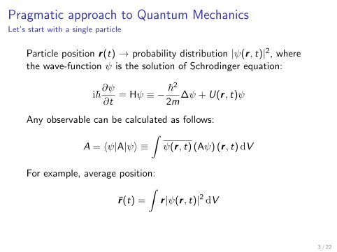
Pragmatic approach to Quantum MechanicsLet’s start with a single particle
Particle position r(t) → probability distribution |ψ(r , t)|2, wherethe wave-function ψ is the solution of Schrodinger equation:
i~∂ψ
∂t= Hψ ≡ − ~2
2m∆ψ + U(r , t)ψ
Any observable can be calculated as follows:
A = 〈ψ|A|ψ〉 ≡∫ψ(r , t) (Aψ) (r , t) dV
For example, average position:
r(t) =
∫r |ψ(r , t)|2 dV
3 / 22

Example: particle in uniform field
Initial conditions (a particle at r0 with velocity ~k/m):
ψ(r , 0) = C exp
[ikr − (r − r0)2
a2
]If U(r , t) = −Fr then
ψ(r , t) ∼ exp
i(k +F t
~
)r −
(r − r0 − ~kt
m −F t2
2m
)2
a2 + i2~tm
=⇒ classical dynamics + gaussian broadening
4 / 22
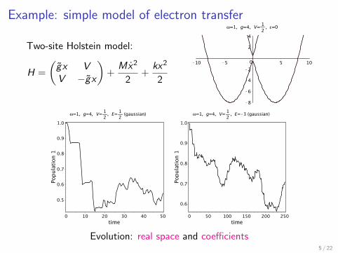
Example: simple model of electron transfer
Two-site Holstein model:
H =
(g x VV −g x
)+
Mx2
2+
kx2
2
Evolution: real space and coefficients5 / 22

Stationary Schrodinger equation
If the Hamiltonian is time-independent then the evolution can bewritten explicitly:
ψ(t) =∑n
cnψne−i En~ t , cn = 〈ψn|ψ(0)〉,
here (En, ψn) are eigenvalues and eigenfunctions of the stationarySchrodinger equation:
Hψ = Eψ
6 / 22

Examples
potential ψn En
free particle eikr ~2k2
2m k ∈ R3
potential box sin πnxa
π2~2n2
2ma2 n = 1,∞
oscillator Hn(ξ)e−ξ2/2 ~ω
(n + 1
2
)n = 0,∞
Coulomb r lL2l+1n−l−1
(2rn
)e−
rnYlm(θ, φ) − α
2an2 n ∈ N,
l < n, |m| 6 l
7 / 22

Practical considerations: basis setPlane waves or atomic orbitals
Wikipedia
8 / 22

Combination of atomic orbitals: examples
9 / 22

Many particle systems: fermions
Slater determinant – basis for many-body systems:
Ψ(ξ1, . . . , ξN) =1√N!
∣∣∣∣∣∣∣∣ψ1(ξ1) ψ1(ξ2) . . . ψ1(ξN)ψ2(ξ1) ψ2(ξ2) . . . ψ2(ξN). . . . . . . . . . . .
ψN(ξ1) ψN(ξ2) . . . ψN(ξN)
∣∣∣∣∣∣∣∣where ψi is i-th orbital and ξj is coordinate+spin of j-th electron.
Methods:
• Hartree–Fock (HF) – take single Slater determinate
• DFT – the same but modify energy functional
• post-HF – expand in basis of finite excitations
10 / 22
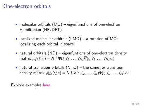
One-electron orbitals
• molecular orbitals (MO) – eigenfunctions of one-electronHamiltonian (HF/DFT)
• localized molecular orbitals (LMO) – a rotation of MOslocalizing each orbital in space
• natural orbitals (NO) – eigenfuntions of one-electron densitymatrix ρ1e
Ψ (ξ; η) = N∫
Ψ(ξ, ζ2, . . . , ζN)Ψ(η, ζ2, . . . , ζN)dζ
• natural transition orbitals (NTO) – the same for transitiondensity matrix ρ1e
ΨΦ(ξ; η) = N∫
Ψ(ξ, ζ2, . . . , ζN)Φ(η, ζ2, . . . , ζN)dζ
Explore examples here
11 / 22

More examples: MO vs NO
HOMO LUMO
ground statenh = 2ne = 0
hole NO electron NO
cation/anionnh/e = 1
∆n2 = .07/.06
singlet excitonnh = 1 + .12ne = 1 − .12
triplet excitonnh = 1 + .17ne = 1 − .18
12 / 22

More examples: NO vs NTO
hole NTO/NO electron NTO/NO
singlet excitonnh = 1 + .12ne = 1 − .12
singlet transitionnh/e = 1 ± .17
triplet excitonnh = 1 + .17ne = 1 − .18
triplet transitionnh/e = 1 ± .25
13 / 22

Strong correlations: Extended Hubbard modelPopulation analysis: ground state, hole, exciton; U/V = 2/1 vs 16/4
Methods: Uniform electron gas approximation for simple metals (LDA)
14 / 22
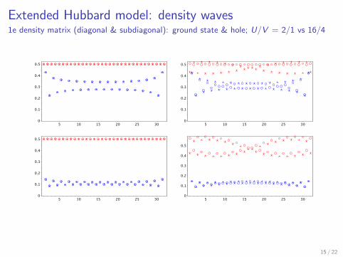
Extended Hubbard model: density waves1e density matrix (diagonal & subdiagonal): ground state & hole; U/V = 2/1 vs 16/4
15 / 22

Quantum mechanics of crystals
Bloch’s theorem for one-electron wave-function:
ψnk(r) = un(r)eikr
where un is periodic, n enumerates electronic bands, k is thewave-vector “periodic” in the reciprocal space define by vectors
bi = eijk2π
υ(aj × ak)
υ = a1 · (a2 × a3) is unit cell volume
16 / 22
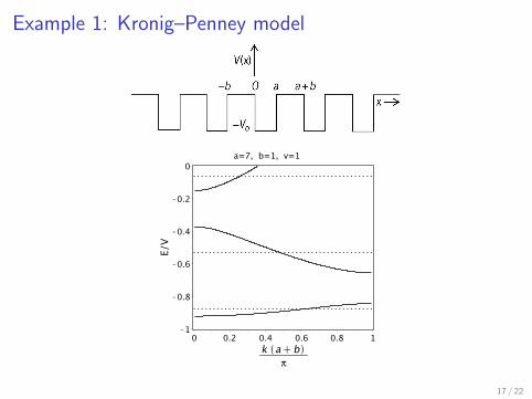
Example 1: Kronig–Penney model
17 / 22

Example 2: Huckel model of trans-polyacetylene
H =
. . .
0 −t1 0−t1 0 −t2
0 −t2 0. . .
ψn = c1,2e
ikn, n ∈ Z, |k | 6 π/2
E (k) = ±√
t21 + t2
2 + 2t1t2 cos 2k
Ebandgap = 2|t1−t2|, Ebandwidth = 2(t1+t2)
18 / 22

Example 2: Total π-electron energy of trans-polyacetylene
Total electronic energy E = 2π
∫ π/20 E (k)dk = −3.34
4x supercell −3.30
19 / 22

Example 3: Silicon crystal
Band structure of Si
L
zk z
Γ
k x
ky
W
VΣ
3X
Λ
∆
KM
Q
1X
U
XS
Σ1
©bilbao crystallographic serverhttp://www.cryst.ehu.esBrillouin zone for Fm-3m
20 / 22

Silicon crystal: charge density
21 / 22
Summary and Resources
See summary here
• Wikipedia
• Bilbao Crystallographic Server
A few textbooks out of many:
• C Kittel, Introduction to Solid State Physics (2005)
• N W Ashcroft, N D Mermin, Solid state physics (1976)
Visualization software:
• Jmol
• Vesta
22 / 22