Electrostatic Properties of Water at Interfaces with Nanoscale Solutes

by

Allan Dwayne Friesen

A Dissertation Presented in Partial Fulfillmentof the Requirement for the Degree

Doctor of Philosophy

Approved July 2012 by theGraduate Supervisory Committee:

Dmitry V Matyushov, Co-ChairC Austen Angell, Co-Chair

Oliver BecksteinVladimiro Mujica

ARIZONA STATE UNIVERSITY

August 2012

ABSTRACT

Molecular dynamics simulations were used to study properties of water at

the interface with nanometer-size solutes. We simulated non-polar attractive

Kihara cavities given by a Lennard-Jones potential shifted by a core radius.

The dipolar response of the hydration layer to a uniform electric field substan-

tially exceeds that of the bulk. For strongly attractive solutes, the collective

dynamics of the hydration layer become slow compared to bulk water, as the

solute size is increased. The statistics of electric field fluctuations at the so-

lute center are Gaussian and tend toward the dielectric continuum limit with

increasing solute size. A dipolar probe placed at the center of the solute is

sensitive neither to the polarity excess nor to the slowed dynamics of the hy-

dration layer.

A point dipole was introduced close to the solute-water interface to fur-

ther study the statistics of electric field fluctuations generated by the water.

For small dipole magnitudes, the free energy surface is single-welled, with ap-

proximately Gaussian statistics. When the dipole is increased, the free energy

surface becomes double-welled, before landing in an excited state, character-

ized again by a single-welled surface. The intermediate region is fairly broad

and is characterized by electrostatic fluctuations significantly in excess of the

prediction of linear response.

We simulated a solute having the geometry of C180 fullerene, with dipoles

introduced on each carbon. For small dipole moments, the solvent response

follows the results seen for a single dipole; but for larger dipole magnitudes, the

fluctuations of the solute-solvent energy pass through a second maximum. The

juxtaposition of the two transitions leads to an approximately cubic scaling of

the chemical potential with the dipole strengh.

i

Umbrella sampling techniques were used to generate free energy surfaces

of the electric potential fluctuations at the heme iron in Cytochrome B562.

The results were unfortunately inconclusive, as the ionic background was not

effectively represented in the finite-size system.

ii

To Darcy

iii

TABLE OF CONTENTS

Page

LIST OF TABLES . . . . . . . . . . . . . . . . . vii

LIST OF FIGURES . . . . . . . . . . . . . . . . . viii

CHAPTER

1 INTRODUCTION . . . . . . . . . . . . . . . . 1

I Electrostatic solvation . . . . . . . . . . . . . . . . . . . 3

A Solvation within linear response . . . . . . . . . . 3

B The solvent as a continuum dielectric . . . . . . . 7

C Success and limitations of continuum electrostatics

for modeling hydration . . . . . . . . . . . . . . . 7

D The importance of electrostatic solvation for spec-

troscopy . . . . . . . . . . . . . . . . . . . . . . . 9

II Polarization of dielectrics . . . . . . . . . . . . . . . . . . 11

III Properties of Water at Interfaces . . . . . . . . . . . . . 17

IV Aspects of the Marcus theory of electron transfer . . . . 21

A Marcus theory . . . . . . . . . . . . . . . . . . . . 21

B Beyond Marcus theory in biological systems . . . 24

2 POLARITY PROFILE OF WATER AT THE INTERFACE WITH

NON-POLAR SOLUTES . . . . . . . . . . . . . . 28

I Introduction . . . . . . . . . . . . . . . . . . . . . . . . . 28

II Structure of the interface . . . . . . . . . . . . . . . . . . 30

III Polarity profile . . . . . . . . . . . . . . . . . . . . . . . 34

IV Dynamics of the hydration layer . . . . . . . . . . . . . . 38

V Electrostatic solvation of dipoles . . . . . . . . . . . . . . 42

VI Discussion . . . . . . . . . . . . . . . . . . . . . . . . . . 44

iv

CHAPTER Page

3 NON-GAUSSIAN STATISTICS OF ELECTRIC FIELD FLUCTUA-

TIONS AT THE SOLUTE-WATER INTERFACE . . . . . 46

I Introduction . . . . . . . . . . . . . . . . . . . . . . . . . 46

II System . . . . . . . . . . . . . . . . . . . . . . . . . . . . 49

III Three-state model . . . . . . . . . . . . . . . . . . . . . . 51

IV Results . . . . . . . . . . . . . . . . . . . . . . . . . . . . 55

V Discussion . . . . . . . . . . . . . . . . . . . . . . . . . . 63

4 COOPERATIVE TRANSITION IN INTERFACIAL WATER . 67

I Introduction . . . . . . . . . . . . . . . . . . . . . . . . . 67

II Results . . . . . . . . . . . . . . . . . . . . . . . . . . . . 68

III Chemical Potential . . . . . . . . . . . . . . . . . . . . . 73

IV Discussion . . . . . . . . . . . . . . . . . . . . . . . . . . 76

5 FREE ENERGY SURFACE OF ELECTRIC POTENTIAL FLUCTU-

ATIONS AT THE REDOX SITE OF CYTOCHROME B562 BY UM-

BRELLA SAMPLING . . . . . . . . . . . . . . . 78

I Introduction . . . . . . . . . . . . . . . . . . . . . . . . . 78

II Results . . . . . . . . . . . . . . . . . . . . . . . . . . . . 79

III Discussion . . . . . . . . . . . . . . . . . . . . . . . . . . 84

6 CONCLUSION . . . . . . . . . . . . . . . . . 86

REFERENCES . . . . . . . . . . . . . . . . . . 89

APPENDIX

A SIMULATION PROTOCOL FOR NON-POLAR KIHARA CAVITIES 95

B SIMULATION PROTOCOL FOR KIHARA CAVITY WITH DIPOLE 98

C THREE-STATE PHENOMENOLOGICAL MODEL . . . . . 100

v

CHAPTER Page

D BOUNDARY VALUE PROBLEM FOR AN OFF-CENTER DIPOLE

INSIDE A SPHERICAL CAVITY IN A DIELECTRIC . . . . 103

E SOLID ANGLE . . . . . . . . . . . . . . . . . 108

F DIPOLAR RESPONSE OF A SUBVOLUME . . . . . . . 110

G SIMULATION PROTOCOL FOR FULLERENE . . . . . . 113

H SIMULATION PROTOCOL FOR CYTOCHROME B562 . . . 115

vi

LIST OF TABLES

Table Page

3.1 List of model parameters produced by fitting the three-state

model to σ2R(m0) from MD simulations. . . . . . . . . . . . . . 55

5.1 Variance of the electric potential at the heme iron for the series

of charge perturbations, δq. The quantities are normalized to

the variance at δq = 0. . . . . . . . . . . . . . . . . . . . . . . 82

5.2 Variance of the electric potential at heme iron, due to all sources

(λvar), water (λvarw ), protein (λvar

p ), and ions (λvarI ), shown for

δq = 0 (RED) and δq = 1 (OX). . . . . . . . . . . . . . . . . . 84

5.3 Contributions to the total Stokes shift from various components

of the system. The subscripts w, p and I refer respectively to

the contributions from water, protein and ions. . . . . . . . . . 84

A.1 Number of hydration waters used in simulations of non-polar

Kihara cavities. . . . . . . . . . . . . . . . . . . . . . . . . . . 96

vii

LIST OF FIGURES

Figure Page

1.1 Marcus parabolas. . . . . . . . . . . . . . . . . . . . . . . . . . 22

2.1 Illustration of the Kihara solute-solvent potential. A Lennard-

Jones shell is added to the surface of a hard sphere of radius

rHS. . . . . . . . . . . . . . . . . . . . . . . . . . . . . . . . . . 29

2.2 Contact values of the solute-solvent pair distribution function. 32

2.3 The first- and second-order orientational order parameters pI1,2

of first-shell SPC/E water vs r0s = rHS + σ0s. . . . . . . . . . . 34

2.4 Dielectric constant of the hydration layer ∆ǫ(r) relative to the

dielectric constant of the same layer around a virtual (Lorentz)

cavity. . . . . . . . . . . . . . . . . . . . . . . . . . . . . . . . 36

2.5 Dielectric susceptibility 4πχ(r)(ρ/ρ(r)) vs the distance r from

the solute center scaled with the water diameter σs. . . . . . . 37

2.6 Exponential relaxation time of χI(t) (filled diamonds), CE(r, t)

(open circles), and χ(r, t) (open squares). . . . . . . . . . . . . 39

2.7 Chemical potential µ∗

d = −µdr30s/(m0)

2 of solvating the point

dipole m0 at the center of the solute of radius r0s. . . . . . . . 43

3.1 Sketch of the standard expectation (a) and the picture proposed

in this study (b) for the free energy of creating field R at a point

within the solute when no dipole is present (equation 3.1). . . 48

3.2 Cartoon of the solute-solvent configuration. The point dipole

m0 is placed at the distance rd from the solute center. . . . . . 50

3.3 Reaction field R0 (in V/A) vs solute dipole m0. . . . . . . . . 51

viii

Figure Page

3.4 Illustration of the phenomenological model we use to under-

stand our results. The surface F (R) is a superposition of a

ground state and two excited states. . . . . . . . . . . . . . . . 53

3.5 Second [pI2, Eq. (3.8)] (main panel) and first [pI1, Eq. (3.7)] (in-

set) orientational order parameters for RD9 (rd = 9 A, filled

squares) and RD10 (rd = 10 A, open squares) configurations. 54

3.6 Free energies F(m0, R) (equation 3.3) for the RD10 state (rd =

10 A) at m0 values indicated in the plots. . . . . . . . . . . . . 57

3.7 The average and variance of the reduced field R∗ as defined by

equation (3.11). . . . . . . . . . . . . . . . . . . . . . . . . . . 58

3.8 Comparison of results with the predictions of linear response

and of continuum electrostatics. . . . . . . . . . . . . . . . . . 60

3.9 Solute-oxygen pair correlation function inside the solid angle. . 61

3.10 Distributions of O-H-O angles. . . . . . . . . . . . . . . . . . . 63

4.1 Average (A) and variance (B) of the reduced solute-solvent,

electrostatic energy u∗

0s. . . . . . . . . . . . . . . . . . . . . . 70

4.2 Non-Gaussian parameter χG = −β〈(δu0s)2〉/〈u0s〉. . . . . . . . 70

4.3 First and second orientational order parameters,pI1 and pI2 for

the first shell waters. The open circles and open squares repre-

sent, respectively the first and second parameters. . . . . . . 71

4.4 Exponential relaxation time, τ2, of the slow component of the

relaxation of the orientational parameter pI1 (solid squares) and

of the electrostatic solute-solvent energy u0s (open circles). . . 73

ix

Figure Page

4.5 Number of waters with oxygen within 8.5 A of the solute center

of mass. The number increases as the system goes through the

crossover, then levels off as the excited state is saturated. . . . 73

4.6 Electrostatic chemical potential of the C180 solute calculated

from thermodynamic integration. . . . . . . . . . . . . . . . . 75

5.1 Free energy surfaces, F (φ) for the RED (δq = 0) and OX (δq =

1.0) states. . . . . . . . . . . . . . . . . . . . . . . . . . . . . . 80

5.2 Free energy surfaces F (φ) for different values of δq. . . . . . . 81

5.3 Distribution of the electric potential at the heme iron for the

RED state (δq = 0). . . . . . . . . . . . . . . . . . . . . . . . 83

5.4 Distribution of the electric potential at the heme iron for the

OX state (δq = 1). . . . . . . . . . . . . . . . . . . . . . . . . 83

E.1 Illustration of the solid angle inside which the distributions were

calculated. The solid angle includes all first shell waters within

an arc length of 2σs of the dipole axis. . . . . . . . . . . . . . 109

x

Chapter 1

INTRODUCTION

Water has long been recognized as important because of its abundance, its

unusual physical properties, and its versatility as a solvent. And while water is

also appreciated as critical to the environment in which all biology takes place,

water is increasingly recognized as a critical active participant in biological

processes at the molecular level[1]. In the area of protein folding, water release

is understood to provide an entropic driving force for folding[2]. And while

the hydrophobic effect is understood to lead to the burying of the protein core,

water also can act as a bridge to form contacts between hydrophilic portions

of the protein[1]. Water has been recognized as critical in determining the

conformational dynamics of proteins[3], and in enzyme function. It can be

critical for structure formation and also for the chemistry, acting as a proton

donor or acceptor[1]. In bioenergetics, water is critical for maintaining proton

gradients [4] and in providing the proper electrostatic environment for efficient

charge transfer[5].

But for all its importance, water is puzzling. The special nature of water is

indicated to first year chemistry students when it is invoked as the “anomalous”

case of a substance that expands on freezing. Water is also famous for its

strangely large boiling point, the density maximum slightly above the freezing

point, and the triple point close to standard conditions. Recently, the nature

of supercooled water has been the subject of much debate[6]. The nature of

the hydrophobic effect and its role in various physical and biological processes

is currently an area of vigorous research[7, 8].

1

In the present work, we will focus on the properties of water at the inter-

face with nanometer-size solutes. Our emphasis will be on the electrostatic

properties of water in such a situation. These properties are essential for un-

derstanding the hydration of solutes with a surface charge distribution, such

as proteins or nanoparticles.

In this chapter, we will present some fundamentals of the electrostatics of

solvation within linear response and within continuum electrostatics. We will

consider the applications of linear solvation for spectroscopy and for electron

transfer in condensed phase. And we will also examine some key properties

of water at interfaces. Once a number of properties of interfacial water have

been outlined, it will come as no surprise that the simple picture of solvation

breaks down for hydration of nanometer size objects.

2

I Electrostatic solvation

A Solvation within linear response

The process of solvating a molecule can be conceptually broken into a

series of steps, each contributing to the total chemical potential of a solute.

The process is commonly separated into 1) the formation of a cavity and 2)

insertion of the solute into the cavity. Depending on the treatment, the third

step of relaxation of the cavity after solute insertion can also be included. In

other treatments, this is considered as part of the second step[9, 10].

The first of these steps is commonly called cavitation, and its contribution

to the total chemical potential is understood as the reversible work required to

exclude the solvent from a volume. This contribution is generally a large, pos-

itive number. The second step involves the formation of solute-solvent interac-

tions, including both long-ranged (electrostatics) and short-ranged (hydrogen

bonds and Van der Waals interactions) forces. This contribution is generally

negative and of similar magnitude to the cavitation free energy. Whether the

chemical potential of a solute is positive or negative depends on the degree of

cancellation between these two terms[9].

In the case of hydrophobic hydration, the cavitation term is the dominating

contribution to the solvation free energy. In recent years, an extensive body of

work has been produced on this subject. We address some of the key results

on hydrophobic solvation in Section 1.3.

In the case of hydrophilic hydration, the formation of solute-water interac-

tions outweighs the cavity-formation work, so that the total chemical potential

is negative. When one considers charge transport or spectroscopic experi-

3

ments, the electrostatic component of the solvation becomes most important.

We focus here on this aspect of hydration.

The electrostatic contribution to solvation thermodynamics of a particle

in a polar liquid can be understood in terms of the solvent response to the

perturbing electric field from the solute. In the absence of a solute charge

distribution (i.e., all solute multipoles zero), the polarization field in the solvent

fluctuates, creating fluctuations of the electric field and the electric potential

inside the solute. The probability distributions of fluctuations of the electric

field and potential are then obtained by projection of the systems many degrees

of freedom onto the electric field or potential in the solute. For the electric

field, the distribution is[11]:

p0(Es) ∝

∫

dΓ e−βH0(Γ)δ3(Es(Γ)− Es), (1.1)

where Es is the electric field produced inside the solute by the solvent, β is

the inverse temperature, 1/kBT , H0(Es) is the system total Hamiltonian, and

δ3(...) is the three dimensional Dirac delta function. and for the statistics of

the electric potential:

p0(φ) ∝

∫

dΓ e−βH0(Γ)δ(φ(Γ)− φ). (1.2)

The probability distributions are related to the reversible work F (Es) and

F (φ) required for a fluctuation of Es or φ from their equilibrium values:

p0(Es) = Q−1e e−βF (Es), (1.3)

and:

p0(φ) = Q−1φ e−βF (φ), (1.4)

where Qe and Qφ are the partition functions,

Qe =

∫

∞

−∞

d3Es e−βF (Es) (1.5)

4

and

Qφ =

∫

∞

−∞

dφ e−βF (φ). (1.6)

If a multipole is placed on the solute, the statistics of the fluctuations are

modified by the electrostatic solute-solvent interaction. For a point charge q,

p(φ) ∝ e−βu0s(φ) × p0(φ), (1.7)

and for a point dipole m,

p(Es) ∝ e−βu0s(Es) × p0(Es). (1.8)

In equations 1.8 and 1.9, u0s represents the solute-solvent electrostatic energy.

In the case of the charge q, we have u0s(φ) = qφ; for dipole solvation, u0s(Es) =

−m · Es.

In the case of linear solvation, the distributions p0(φ) and p0(Es) are Gaus-

sian, with the width of the fluctuation spectrum determined by the response

function κi,where i = q or i = m indicates the response to a charge or dipole,

respectively[12]:

p0(φ) ∝ exp(−βφ2/2κq) (1.9)

and

p0(Es) ∝ exp(−βE2/2κm). (1.10)

The variances are:

〈(δφ)2〉 = κq/β (1.11)

and

〈(δEs)2〉 = 3κm/β. (1.12)

If the fluctuations are Gaussian, the effect of the multipole is simply to shift the

distribution by the amount −κqq or κmm. The average solute solvent energy is

5

then u0s = −κmm2 for a dipole and u0s = −κqq

2 for a charge. Because of the

connection of the response function κi to both the fluctuations and the average

of the energy, one can relate the solute-solvent energy u0s to the fluctuations

of the field or of the potential with the multipole not present. For a charge,

〈u0s〉 = q〈φ〉 = −βq2〈(δφ)2〉0 (1.13)

and for a dipole,

〈u0s〉 = −〈m · Es〉 = −βm2

3〈(δEs)

2〉0. (1.14)

In equations 1.13 and 1.14 〈...〉0 indicates the average taken in the ensemble

with zero multipole. Deviations from Gaussian statistics can then be quantified

in terms of the nonlinear parameter,

χG = −β〈(δu0s)

2〉

〈u0s〉, (1.15)

equal to 1 when the fluctuations are Gaussian. The electrostatic contribu-

tion to the solvation free energy can then be found from thermodynamic

integration[13]. For a point charge, we have:

µq =

∫ q

0

dq′⟨

∂u0s

∂q

⟩

= −

∫ q

0

dq′ κqq′ = −

κq

2q2 = 〈u0s〉/2. (1.16)

Similarly, for a point dipole:

µm = −κm

2m2 = 〈u0s〉/2. (1.17)

In calculating the chemical potential, it is not necessary to include the con-

tributions from solvent-solvent interaction, because the entropic and energetic

contributions to the free energy from the solvent exactly cancel[14].

6

B The solvent as a continuum dielectric

For a spherical ion with radius r0s, if the solvent is modeled as a dielectric

with dielectric constant ǫ, one can calculate the electrostatic work for charging

up the solute by integration of the energy density over the solvent volume [15]:

w =(ǫ− 1)

8π

∫

∞

r0s

dr 4πr2E(r)2. (1.18)

The chemical potential for the point charge is then given by the familiar Born

equation[16]:

µq =

(

1

ǫ− 1

)

q2

2r0s. (1.19)

For a spherical solute with a dipole at the center, solution of the Poisson

equation with the Maxwell boundary conditions gives the solvation chemical

potential as[17, 18]:

µm =(ǫ− 1)

2ǫ+ 1

m2

r30s. (1.20)

A derivation of equation 1.20 is given in Appendix D. The response func-

tion from the linear response formalism can then be related to the dielectric

constant of the solvent:

κq =1− ǫ

ǫr20s(1.21)

and

κm =2(ǫ− 1)

2ǫ+ 1

1

r30s. (1.22)

C Success and limitations of continuum electrostatics for

modeling hydration

The Born equation has been reported to work for ion solvation, provided

certain corrections are applied[19]. It is found that in simulations of neutral

(“empty”) cavities, the potential inside the solute is positive [19, 20, 21]. As

7

a result, even if the solvent response to the charge in a cavity is harmonic,

it is harmonic about a non-zero value of the solute charge. The consequence

of this is that hydration of negative ions is more favorable than hydration

of positive ions of the same size and charge magnitude. This can be traced

back to the difference in hydration structure around positive and negative

ions[19]. The effect has been noted in several simulation studies, and is also

seen experimentally[22].

Similarly, the expected scaling is found for a dipolar sphere solvated in

water, as long as the dipole is not too close to the interface (see Chapter

2)[23]. However, it has also been shown that for a hard cavity in a fluid of

dipolar hard spheres, the chemical potential of a dipole placed at the center of

the cavity scales much more strongly with the cavity radius than continuum

models would predict[12].

It should be noted that the scaling of the solvation energy with the squared

multipole is only a confirmation of linear response, since the continuum radius

of the solute and the dielectric constant of the solvent also come into the pic-

ture. Estimation of the particle radius is problematic, since real solutes are not

hard cavities, but soft particles. As a result, what generally happens is that

the continuum radius is chosen from some sort of fitting that involves a former

supposition of the applicability of continuum electrostatics[20, 24]. In simula-

tions employing continuum electrostatics, the parameters are sensitive to the

details of the forcefield[24]. Furthermore, since many studies are focused on

water, it is difficult to check the predicted dependence of the hydration energy

on the dielectric constant of the solvent; the dielectric constant is somewhere

between about 70 and 80 for water at most temperatures of interest[25], so

8

that the factor 1− 1/ǫ is approximately 1. The same is true for the factor in

the Onsager equation, 2(ǫ− 1)/(2ǫ+ 1).

D The importance of electrostatic solvation for spectroscopy

When an optical probe absorbs a photon in the gas phase, the charge

distribution and molecular geometry change, corresponding to the change of

quantum state. The line shape of an electronic transition acquires a fine struc-

ture due to the transitions to the various possible vibrational states. Assuming

that the electronic matrix element does not change with the nuclear coordi-

nates, the probability of landing in a given vibrational state is determined by

the Franck-Condon (FC) factor:

|〈χi,a|χf,b〉|2, (1.23)

where χa,i is the nuclear wavefunction in electronic state i at the vibrational

level a, and χf,b is the same quantity for final electronic state, f and vibrational

state b. The (FC) factor then is the squared overlap integral between the

two vibrational wavefunctions[26, 27]. Immediately following the transition,

the nuclear coordinates are generally out of equilibrium, and the molecular

geometry will rearrange, dissipating the energy λv.

If we consider now a chromophore in solution, the many solvent vibrational

modes become important to the energetics. The probability of an electronic

transition then depends on the statistical average of the FC factor over the

vibrational states[27, 28]:

F (Ei,f ) =1

Qi

∑

i,f

e−βEi,a|〈χi,a|χf,b〉|2δ(Ei,f + Ei,a − Ef,b), (1.24)

where

Qi =∑

a

e−βEi,a . (1.25)

9

One gets a significant broadening of the line shape, due to the coupling of the

electronic transition to the solvent modes[29, 28].

The reversible work associated with the rearrangement of the solvent nu-

clear coordinates in response to the change in electronic structure of the solute

is called the solvent reorganization energy, λs. The solute is typically modeled

as a spherical cavity in a dielectric solvent, with a dipole at the center. The

change of electronic state then corresponds to a change in the solute dipole mo-

ment. Within this model, the solvent reorganization energy (or outer sphere

reorganization energy) λs is related to the change in solute dipole moment

∆m0, the cavity radius R0s, and the dielectric constant of the solvent ǫ[30].

λs =(∆m0)

2

(R0s)3

(

ǫ− 1

2ǫ+ 1−

n2 − 1

2n2 + 1

)

. (1.26)

In equation 1.26, the squared refractive index n2 refers to the solvent response

on optical timescales. This is subtracted out, since we are concerned here

with the relaxation of nuclear modes. In this model, the solvent response is

harmonic, so that the reorganization energy for forward and reverse transitions

is identical.

We define the vertical energy gap X, the reversible work required to change

the electronic state with all nuclear modes frozen. The Stokes shift ∆X is

then the difference in the energy gap between forward and reverse transitions.

Within linear response, conservation of energy requires:

∆X = 2(λs + λv) = 2λ. (1.27)

The relation of the energy gap to the Stokes shift will be addressed in more

detail in the discussion of electron transfer in section IV.

Within linear response, the solvent response to changing dipole moment is

also related to the fluctuations of the electric field at the solute, within one

10

electronic state. The solvent contribution to the linewidth is then related to

the solvent reorganization energy[28]. Neglecting the vibrational contribution,

β

2〈(δX)2〉 =

∆X

2= λs. (1.28)

II Polarization of dielectrics

We present here a brief discussion of polarization in dielectrics. In macro-

scopic electrodynamics, the medium is treated as a continuum, with molecular

details coarse-grained. Rather than treating the highly heterogeneous micro-

scopic electric field, for example, we work with the average field E, commonly

called the Maxwell field[31]. The polarization field is handled similarly. The

line of reasoning followed here is abstracted from the arguments found in the

treatments by Landau[31], Frohlich[15] and Bottcher[18].

We begin with the postulate that the electric field flux through any closed

surface is equal to the charge enclosed in that surface (Gauss’s law):

∮

ds E = 4πe, (1.29)

where e is the enclosed charge, and the integral is taken over the whole surface.

In differential form, equation 1.29 can be written as:

div E = 4πρ, (1.30)

where ρ is the charge density. The electric field E is also assumed to be the

gradient of a scalar potential field φ, satisfying the condition,

curl E = 0. (1.31)

With these assumptions, we can now write,

E = −grad φ. (1.32)

11

So we recognize the electric field as the gradient of the electric potential.

Consider a conducting body placed in a uniform electric field, E0. The

charge distribution on the conductor will arrange so that at all points on the

conductor, the electric field E is zero. The argument for this is simple: a non-

zero electric field will generate a force on any charge in the medium. Since

charges in conductors are free to flow, the charge will move until the net force

on the charge is zero. Furthermore, since any charge inside the body is itself a

source of field, the entire charge distribution must go to the surface[31]. The

result is a surface charge density σ (charge per unit surface area) given by:

4πσ = E0,n, (1.33)

where E0,n = E0 · n is the the projection of the electric field on the surface

normal.

If one considers a dielectric instead of a conductor, the situation is different.

In a dielectric, charges are bound, so that the body cannot carry a current.

However, the dielectric will polarize in the presence of an external field. This

is quantified by the polarization field P, equal to the dipole moment per unit

volume. The polarization field contributes a charge density −div P = ρ.1 It

is instructive to consider the case of a planar interface of the dielectric with

the vacuum, in a uniform external field oriented along the surface normal. A

uniform polarization is induced in the dielectric, so that at all points inside

the dielectric, div P = 0. However, at the boundary, the polarization of

the dielectric creates an apparent surface charge density, equal to the normal

1In a rigorous treatment, the polarization field is typically first defined as the vector field

with divergence equal to the charge density: −div P = ρ. It is only after the observation

that integration of −r div P over space produces the macroscopic dipole moment that we

are compelled to identify the polarization field with the dipole moment per unit volume[31].

12

component of the surface polarization, Pn = P · n:

σ = Pn. (1.34)

The apparent surface charge contributes an amount to the total electric field

in the dielectric equal to:

∆E = −4πσ n = −4πP. (1.35)

The consequence of this is that the electric field is partially screened by the

polarization of the dielectric. For modest external fields, the field inside the

body is reduced compared to the vacuum field by the proportionality factor

1/ǫ:

E =1

ǫE0. (1.36)

The associated difference in electric field across the interface is then:

∆E =

(

1

ǫ− 1

)

E0. (1.37)

In the linear regime, the polarization in the dielectric is proportional to the

electric field. Introducing the dielectric susceptibility, χ we have:

P = χE. (1.38)

Comparison of equations 1.35, 1.37 and 1.38, gives the relation of the dielectric

susceptibility to the dielectric constant, χ = (ǫ− 1)/4π, and we find:

P =ǫ− 1

4πE. (1.39)

Because the electric field inside a dielectric is screened by the polarization,

it is useful to consider the vector field D, called the electric displacement, that

reflects only the field due to free (or “true”) charges:

D = E+ 4πP. (1.40)

13

In the linear regime, we have the simple relationship, D = ǫE. Under this

circumstance, Gauss’s law for free charges becomes:

div D = 4πρf , (1.41)

Combining equations 1.41 and 1.32, we obtain Poisson’s equation for a linear,

homogeneous dielectric:

ǫ∆φ = 4πρf . (1.42)

At the boundary between two regions of space with differing dielectric con-

stant, one applies the boundary conditions requiring the continuity of the po-

tential φ and the discontinuity of the normal component of the electric field:

φ1 = φ2 (1.43)

and

ǫ1∂φ1

∂r= ǫ2

∂φ2

∂r. (1.44)

Moving from a continuum description to a statistical mechanical picture,

we now consider the fluctuations of the total dipole moment M =∫

dV P of a

dielectric. For simplicity, we take any external field to be along the z direction:

E0 = E0 · z = |E0|. We focus on the statistics of the z projection of the dipole

moment M = M · z. In the absence of an applied field, the statistics of the

fluctuations will be given by the distribution:

p0(M) ∝

∫

dΓ e−βH0(Γ)δ(M(Γ)−M), (1.45)

whereH0(Γ) is the total Hamiltonian of the system at point Γ in phase space, in

the absence of an applied field. The introduction of the external field modifies

the system Hamiltonian to:

H(Γ, E0) = −ME0 +H0(Γ). (1.46)

14

Correspondingly, the distribution of dipoles becomes:

p(M) ∝ eβME0p0(M). (1.47)

The average dipole of the material is given by the statistical average,

〈M〉 = Q−1

∫

dΓ eβME0−βH0(Γ)M, (1.48)

where

Q =

∫

dΓ e−βH(Γ,E0). (1.49)

Differentiating, we obtain (see Appendix G for details):

∂〈M〉

∂E0

=β

V〈(δM)2〉. (1.50)

Including fluctuations of the x and y components of the system dipole, we get:

∂〈M〉

∂E0

=β

3V〈(δM)2〉. (1.51)

The dielectric constant is then given by (see equation 1.39) [18]:

ǫ− 1

4π=

β

3V〈(δM)2〉 ×

∂E0

∂E. (1.52)

To determine the dielectric constant, it is necessary to work out how the

external fieldE0 is related to the Maxwell fieldE. This is a non-trivial problem.

One can consider a spherical cavity carved from a dielectric, in an exter-

nal field, E0. Solution of the Poisson equation with the standard boundary

conditions yields the cavity field,

Ec =3ǫ

2ǫ+ 1E, (1.53)

so that the external field is reduced by the factor, 3/(2ǫ+ 1). If one now

inserts the dielectric back into the cavity, one can calculate the electric field

15

generated inside the sphere due to the polarization of the surroundings by the

charge distribution in the sphere. This field is called the reaction field and was

first calculated by Onsager[17]:

R0 =2(ǫ− 1)

2ǫ+ 1

Ms

a3, (1.54)

where Ms is the total dipole moment in the spherical region and a is the

radius of the spherical region. If the polarization inside the sphere is given by

P = (ǫ− 1)/4πE, then we have:

M =(ǫ− 1)a3

3E. (1.55)

The total field acting on the spherical region from outside sources is then the

sum of the cavity field and the reaction field:

Ee = Ec +R0 =ǫ+ 1

3E. (1.56)

Equation 1.56 can be derived by a number of routes. We have taken the present

approach to demonstrate the distinction between the total field from outside

sources, Ee and the “directing” field[18] (the portion of Ee that contributes

to the polarization in the subvolume). Since the reaction field orients always

along the dipole moment of the subvolume under consideration, it does not

contribute to the orientational statistics of the subvolume. Then for a spher-

ical subvolume, the appropriate directing field is given by the cavity field in

equation 1.53. We have for the factor in equation 1.52:

∂E0

∂E=

Ec

E=

3ǫ

2ǫ+ 1. (1.57)

Using equation 1.57 in equation 1.52 we obtain Kirkwood’s formula for the

dielectric constant[32, 18]:

(ǫ− 1)(2ǫ+ 1)

12πǫ=

βN

3Vgµ2, (1.58)

16

where µ is the permanent dipole of a single molecule, N is the total number

of molecules in the subvolume and g is called the Kirkwood factor, given by:

g =〈M2〉

Nµ2. (1.59)

This equation is valid in the limit of a very large system. In practice, on the

length scales used in computer simulations, and due to the boundary con-

ditions when handling long range forces, it is necessary to apply corrections

when the Kirkwood factor is calculated for finite volumes[33]. In the case of

simulations performed with tinfoil boundary conditions one obtains for the

dielectric constant[34, 33]:

ǫ = 1 +4πβ

3V〈(δM)2〉. (1.60)

III Properties of Water at Interfaces

The properties of water as a solvent are determined by a combination of

short-ranged hydrogen bonds and dispersion forces and long-ranged electro-

static interactions. When a nano-sized object is inserted in water, both the

density profile of water and the hydrogen bond distribution are significantly al-

tered. The orientational properties of water at interfaces are then determined

by a competition between water-water hydrogen bonds and solute-solvent in-

teractions, and therefore by the character of the solute-solvent potential, such

as whether the solute is hydrophobic or hydrophilic[35, 36].

Because of water’s preference for locally tetrahedral structure, the distri-

bution of water’s hydrogen bond network can be reduced to a combination of

preferred orientational states at the interface [35, 37, 38]. When the interface

is repulsive or only weakly attractive, the dominant configuration of interfacial

waters is an ice-like structure with one unsaturated hydrogen bond pointed to-

17

ward the interface, along the normal; there is also a contribution from waters

with their dipoles pointed in the plane of the interface[35]. The distribution of

protons in this picture is essentially random, with some unsaturated H-bond

donors and some H-bond acceptors pointed toward the surface.

When the solute-solvent attraction is increased, the pulling force from the

surface causes a repopulation of the orientational states, causing a shift in

the mean orientations, but without a significant change to the preferred ori-

entations themselves [37]. When modest surface charges are introduced, the

increased solute-solvent attraction is balanced by the increased possibility of

forming hydrogen bonds in a more densely packed interface, so that the overall

result is a dominantly in-plane orientation of water dipoles. The fundamental

reason behind this phenomenology is the large (∼ 4kT ) energy of hydrogen

bonds in water. Because of these strong forces, the structure of the hydra-

tion shell is extremely resilient to external perturbations, which generally only

cause repopulation of the different preferential surface configurations.

In contrast, for highly charged surfaces, such as at the silica-water interface,

it is found that the dominant orientational state of water is actually opposite

that found at hydrophobic interfaces, with the water dipoles pointed along the

interface normal. This was originally found in molecular dynamics simulations,

and was eventually confirmed experimentally[39, 40]. Because water is both

strongly dipolar and strongly quadrupolar, the orientational properties of the

interface also affect the water’s electrostatic properties. This is relevant for

understanding the electrostatics of hydration, both in terms of the long-range

dipolar response of the solvent, as well as the fields generated from the higher

multipoles of water, on shorter length scales.

18

In hydrophobic solvation, it has been shown that small solutes inserted into

water cause little disruption to the hydrogen bond network. Consequently, the

hydration free energy in such cases turns out to be controlled by the solute

volume and the solvent compressibility[41, 42]. However, the hydrogen bond

network is disrupted at more extensive interfaces. One therefore expects at

some length scale a crossover between two types of hydrophobic hydration.

Such a crossover was predicted in the Lum-Chandler-Weeks (LCW) theory

of hydrophobic hydration[43]. The theory predicts that for solvation of small

hard cavities in water, the hydration free energy should scale as R30s. If the

solute size is increased, at solute radii slightly larger than one solvent diameter,

a crossover occurs, and the free energy of hydration then scales as R20s. The

crossover is associated with a transition from “volume dominated” to “surface

dominated” hydration[12].

The LCW theory also predicts a drying of the solute-water interface for

solutes larger than the crossover length scale, so that for large hydrophobes the

structure of the interface is closer to the water-vapor interface[43]. In practice,

what is observed around weakly attractive hydrophobic solutes in water is a

“weak dewetting” of the interface[44]. In this phenomenology, the contact

value of the solute-water pair correlation function first increases with solute

size, for small cavities, then reaches a maximum at the point of the crossover

[45, 8].

The common explanation for these observations is that a change occurs in

the nature of water’s hydrogen bond network near the interface, with most

hydrogen bonds preserved for small solutes, and with a substantial surface

disruption of the network for larger solutes[12, 39]. While this is compelling,

the situation may not be so simple. It was shown that a similar crossover

19

occurs for hard cavities in a dipolar hard sphere fluid[12]. In this case, there

are no hydrogen bonds, and the crossover might be understood in terms of a

change in the orientational ordering of the dipoles at the interface. In both

the case of dipolar hard spheres and hydrophobic cavities in water, the contact

value of the solute-water pair correlation function reaches a maximum around

the crossover, although the transition occurs at different length scales [12, 46].

The dynamics of water at microscopic length scales have been tradition-

ally probed by Stokes-shift dynamics[47]. The dynamics of the energy gap X

between ground and excited states of a chromophore is monitored. The infor-

mation on relaxation is then obtained by means of the Stokes shift correlation

function:

C(t) =〈δX(t)δX(0)〉

〈(δX)2〉. (1.61)

The Stokes shift dynamics for free chromophores in water are found to decay

on timescales faster than 1 ps. However, when chromophores are bound to

proteins in solution, long tails appear, relaxing on timescales ranging from

several 10s of ps[48, 49] to ns [50]. The cause of this effect has been the

subject of some debate, with some claiming there is an intrinsically very slow

property of hydration water seen in the Stokes shift, and with others assigning

the slow dynamics to coupling of hydration waters to slow protein modes[48,

51]. The issue is clouded by the fact that the hydration dynamics cannot

be separated from the complex protein dynamics. This raises the question of

what is actually probed by the Stokes shift. Since dielectric models suggest

that the Stokes shift probes the solvent response at very long length scales, one

wonders whether Stokes shift spectroscopy is an appropriate probe for local

hydration dynamics.

20

IV Aspects of the Marcus theory of electron transfer

A Marcus theory

By far, the most widely known and applied theory of electron transfer in

condensed phase is the Marcus formalism. Marcus divides the response to a

change of electronic state into two parts, called the inner and outer spheres.

The inner sphere is the redox site and anything bound to it; this includes co-

valently bonded atoms, ligated atoms and tightly bound solvent molecules. In

the case of a self exchange reaction between two ions such as Fe2+ and Fe3+,

the inner sphere would include the ion plus a first layer of hydration waters,

assumed to be dielectrically saturated[52, 53]. Whatever is outside this layer

constitutes the outer sphere, and is assumed to behave like a dielectric in the

linear regime. Marcus observed that for such reactions the main contribution

to the free energy typically comes from the outer sphere, due to the long range

of electrostatic forces, and the early theory development was for reactions in

which the energetics were dominated by the outer sphere, although Marcus

recognized early on that this simplification was not robust[53]. The theory

has since been extended to include contributions from the inner sphere. In

that case, the inner sphere is assumed to comprise another harmonic contri-

bution, uncoupled from the outer sphere[54]. Accordingly, one expects the

Marcus theory not to apply to cases in which linear response fails or when

the distinction between inner and outer spheres becomes unclear (for example

because of binding/unbinding events, such as proton transfer)[55].

In order to formalize the electron transfer problem, an appropriate reaction

coordinate must be chosen that projects the coordinates of all nuclei onto a

single scalar quantity. In his original treatment, Marcus used the charge at

21

the redox site as a reaction coordinate. Marcus then calculated the free energy

required to create the polarization that would correspond to the equilibrium

polarization about the activated complex, with the electron charge divided be-

tween donor and acceptor[52, 56]. The problem was eventually put on a firmer

foundation by using the vertical energy gap (energy difference between the two

redox states with all nuclear coordinates frozen) as the reaction coordinate[57].

This quantity is proportional to the electric potential at the redox site, and

therefore to the charge, within linear response, so that the difference between

the two is purely formal. However, if the solvent response becomes nonlinear,

the distinction can become more important[58]. The energy gap X as a reac-

tion coordinate reflects the requirement of crossing the Franck-Condon barrier

at X = 0.

X0,i 0 X

0,f

F(X

)

∆F

λλ

F*

∆X = 2λ

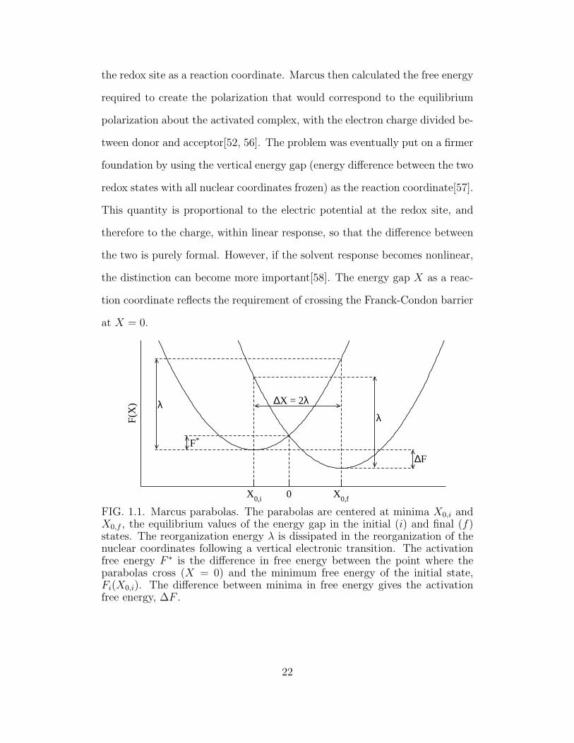
FIG. 1.1. Marcus parabolas. The parabolas are centered at minima X0,i andX0,f , the equilibrium values of the energy gap in the initial (i) and final (f)states. The reorganization energy λ is dissipated in the reorganization of thenuclear coordinates following a vertical electronic transition. The activationfree energy F ∗ is the difference in free energy between the point where theparabolas cross (X = 0) and the minimum free energy of the initial state,Fi(X0,i). The difference between minima in free energy gives the activationfree energy, ∆F .

22

Marcus treats the outer sphere response as a dielectric in the linear regime.

As a result, the free energy surfaces obtained for fluctuations along the reaction

coordinate are harmonic. The problem is then set up as two crossing parabolas,

with the energy gap X as the reaction coordinate. In figure 1.1, the parabola

on the left Fi(X) represents the free energy in the initial state and Ff (X)

on the right represents the final state. Their minima are at X0,i and X0,f ,

respectively. The vertical distance between the two minima is the free energy

driving force for the reaction, ∆F . To understand the energetics of the electron

transfer, we break the process into two steps. First, the nuclear coordinates

are frozen, and the electronic state is changed from the initial state to the final

state. This costs the amount of work X0,i. Second, the nuclear coordinates are

relaxed to the equilibrium point for the final electronic state; the amount of

energy dissipated in this process λs is known as the outer shell reorganization

energy or the solvent reorganization energy. The total reorganization energy λ

includes contributions from the inner sphere as well. However, in the present

discussion, we consider only the contribution from the solvent. The total free

energy change for the sum of these two processes gives the driving force for

the reaction,

∆F = X0,i − λs. (1.62)

For a radiationless electronic transition to occur, one requires that the vertical

energy gap be zero. Accordingly, the transition state occurs at the point where

X = 0, where the two parabolas cross. The free energy barrier to the reaction

is then:

F ∗ = Fi(0)− Fi(X0,i) = Ff (0)− Ff (X0,f ) + ∆F. (1.63)

23

The two parabolas in figure 1.1 must have the same curvature within linear

response. Consequently, the reorganization energy is the same for forward and

reverse reactions. Conservation of energy then requires that

−X0,i − λs +X0,f − λs = 0. (1.64)

so that the Stokes shift ∆X = X0,f − X0,i is related to the reorganization

energy. The condition of linear response further relates the Stokes shift ∆X

to the variance of the energy gap. We get the relations:

∆X = 2λs = β〈(δX)2〉. (1.65)

We will denote the reorganization energy calculated from the stokes shift as

λSt, and the reorganization energy from the variance, λvar. The two are equal

only when the statistics of the energy gap fluctuations are Gaussian. We can

then evaluate the degree of non-Gaussianity in electron transfer in analogy

with equation 1.15: χG = λvar/λSt.

Once the relationship between λs and ∆X has been established, one can

use simple algebra to find the point of intersection of the two parabolas. Then,

for the activation free energy, we get:

∆F ∗ =(λs +∆F )2

4λs

. (1.66)

B Beyond Marcus theory in biological systems

The limitations imposed by the assumption of linear response in the Marcus

theory are quite stringent. The result of linear response is the connection

between the reorganization energy λs, the free energy of reaction ∆F and the

activation barrier, F ∗ indicated by equation 1.66. The consequence is that for

a redox reaction to proceed very quickly (to have a small free energy barrier),

24

one must have a reorganization energy comparable in size to the driving force

for the reaction. Literature calculations of the reorganization energy for redox

proteins involved in photosynthesis suggest that values of λs are typically

on the order of 0.5 eV, although measurements[59, 60] and calculations [61]

produce a range of estimates ranging between 0.1 eV and 1.0 eV[62]. The

energy input in photosynthesis is about 1.4 eV after which several electron

hops are necessary in order to store the energy [63, 62]. In each step, free

energy driving force for each of these hops is estimated to be around 0.7 eV

[64]. The question arises of how the biological system has any energy left,

after the several redox processes occur. These reactions are generally quite

fast. Once a photon is absorbed, the initial electron transfer step happens

with better than 99% efficiency. This implies a very small free energy barrier

for the reaction. Thus, one expects to dissipate about half an electron volt

for each hop. In this picture, the entire photon energy is lost in about three

hops. It has been suggested that the reorganization energy for electron transfer

in the initial events of photosynthesis was actually significantly smaller than

what is usually reported from experiments [65, 66]. It was further pointed

out[66] that the relevant reorganization energy for biological electron transfer

might not involve all the equilibrium fluctuations of the energy gap, since

these motions will be frozen on the timescale of electron transfer. This was a

reasonable solution to the problem of the thermodynamics of photosynthesis,

but neglected the fact that a very small reorganization energy, within the

standard picture, will lead to very slow reaction rates, and that the freezing

out of fluctuations eventually leads to dynamical arrest of electron transfer[67].

Eventually, work by David LeBard and Dmitry Matyushov on photosyn-

thetic systems[62, 5, 63] showed that, in fact, when long trajectories are avail-

25

able, one actually calculates a reorganization energy several times larger than

what is typically reported for experiment. Interestingly, this finding was up-

held only when the reorganization energy was calculated from the variance of

the potential:

λvar =β〈(δX)2〉

2. (1.67)

Within the linear response formalism, this is equivalent to the reorganiza-

tion energy calculated from the Stokes shift:

λvar = λSt = ∆X/2. (1.68)

What was found, however, is that the reorganization energy from the fluc-

tuations is several times larger than the reorganization energy from the Stokes

shift. The implication is that linear response, and therefore the Marcus the-

ory, does not apply in these systems. In the case of plastocyanin, it was

found further that when the observation window was narrowed to ∼ 100 ps,

the prediction of linear response was approximately restored. The degree of

nonlinearity can be quantified through the use of the parameter χG, equal to

1 when fluctuations are Gaussian. This parameter was found to be of order

3 to 10 for reduction of plastocyanin and for the reactions in the bacterial

photosynthesis reaction center[62, 5, 63].

The emerging picture is that biological energy chains may circumvent the

limitations of the standard picture of electron transfer in two ways. First, the

fluctuations of the electric potential at the redox site seem to be much larger

than previously expected, and are non-Gaussian. This allows the breaking of

the requirement connecting the free energy barrier to the reaction free energy.

In this picture, the variance of the energy gap X is quite large, corresponding

to a broad shape of the electron transfer free energy surfaces, near the minima,

26

leading to small activation barriers. However, the Stokes shift remains small,

so that not much energy is dissipated when the electron is transferred[63].

The second point is that the large fluctuations associated with λvar are

associated with slow hydration dynamics. The slow component of the fluc-

tuations does not relax on the timescale of electron transfer, so that while

the large fluctuations lead to broad free energy surfaces, allowing fast electron

transfer rates, very little energy is actually dissipated in the redox process [62].

The nature of the slow dynamics is not entirely clear, but it seems to be due

in part to hydration water coupling to protein slow modes and in part to some

intrinsically slow dynamics of water at the interface [68].

27

Chapter 2

POLARITY PROFILE OF WATER AT THE INTERFACE WITH

NON-POLAR SOLUTES

I Introduction

To begin to address the gap between the formalism of Maxwell’s continuum

electrostatics and the situation for solutions of polar liquids, we used molecular

dynamics simulations of model solutes to study the polarity profile of hydration

shells around spherical hydrophobic solutes. Hydrophobic solvation has been

the subject of extensive research in recent years, with emphasis on properties of

the interface such as the density profile [46, 69], the thermodynamics of cavity

formation [70] and the compressibility of hydration shells [8]. Little work has

been done, however, on the electrostatic properties of hydration layers. Given

the strong distortions to the density profile and the orientational structure of

water at the interfaces with large solutes, in the present study, we sought to

address the question of how the electrostatic properties of the hydration layer

are affected.

Therefore, in contrast to existing work in this field [71, 69, 8, 46, 72], we

asked the following questions: (i) how polar is the interface? (ii) how are

the collective dipolar dynamics of the hydration layers affected by the solute?

(iii) how are the dynamics of the hydration layer perturbed by the solute,

and how far does the structural and dynamical perturbation penetrate into

the solvent? (iv) are perturbations of interfacial water dynamics visible in the

28

r0s

rHS

!s

!0s

rSPC/E

watersolute

FIG. 2.1. Illustration of the Kihara solute-solvent potential. A Lennard-Jonesshell is added to the surface of a hard sphere of radius rHS. The approximateposition of the first peak of the solute-water pair distribution function is r0s =rHS + σ0s. The dielectric constant in Eq. (2.5) is calculated from the dipolemoment of waters located between the spheres of radii r0s and r shown in thegraph.

Stokes-shift dynamics[47, 48]? and (v) for what solute size does the interfacial

polar response approach the limit of continuum Maxwell electrostatics?

We represented the interaction between the solute and water oxygen using

the Kihara potential[73, 74], which is equivalent to the Lennard-Jones poten-

tial, shifted by the core radius rHS:

φ0s(r) = 4ǫ0s

[

(

σ0s

r − rHS

)12

−

(

σ0s

r − rHS

)6]

. (2.1)

In this equation, σ0s is the width of the solute-solvent Lennard-Jones in-

teraction, ǫ0s is the depth of the potential energy well, and r is the distance

from the solute center to the water oxygen. The closest approach (first peak

of the pair correlation function) of the water oxygen is then approximately

r0s = rHS +σ0s. The water-water interactions were represented by the SPC/E

potential [75]. The system with these parameters is illustrated in figure 2.1.

The solute size was varied from atomic-sized to nanoscale by varying the

hard radius rHS between 0 and 12 A. We studied systems with two different

Lennard-Jones energies for the solute-solvent attraction. At the hydropho-

bic extreme, we studied the system with ǫ0s = 0.65 kcal mol−1, equal to the

Lennard-Jones energy of SPC/E water. Then at an opposite extreme, we stud-

29

ied systems with ǫ0s = 20 kcal/mol, comparable to the hydrogen bond energy

of water.

The number of waters in the simulation box was varied to allow sufficiently

thick hydration layers. For the smallest solutes, 4053 waters were included in

the simulation cell, and for the largest system, 11845 water molecules were

used. Systems were simulated by molecular dynamics using DLPOLY[76] at

constant temperature and pressure for 5 ns, following 100 to 500 ps equili-

bration. A timestep of 2 fs was used and the temperature and pressure were

maintained at 273 K and 0 atm using the Berendsen thermostat and barostat.

Cubic periodic boundary conditions were used, and the electrostatics were

handled using Ewald summation. Further simulation details are compiled in

Appendix A.

II Structure of the interface

In order to understand how our model system compares to systems already

in the literature, we examined the contact value of the solute-water radial

distribution function and the compressibility of the first hydration shell. We

defined the first hydration shell as including waters within the distance, r ≤

r0s + σ0s + σs/2, where σs is the effective hard sphere diameter of water, 2.87

A[77]. This cutoff is approximately the location of the first minimum of the

solute-solvent pair correlation function.

To study the compressibility of the first hydration shell the quantity κI =

〈(δN)2〉/〈N I〉 was calculated, whereN I is the number of water molecules in the

first hydration shell. In the thermodynamic limit, the variance of the number of

particles is related to the isothermal compressibility by χT = βV 〈(δN)2〉/〈N〉

[13]. The quantity κI has been reported for a variety of solutes in water. The

30

compressibility of hydration shells has also been connected with protein de-

naturation. The typical result for hydrophobic solutes it that as the solute

size is increased, the hydration layer becomes increasingly compressible, with

κI passing through a minimum for solutes of modest size, with radius ∼3 A.

The large compressibility of hydration shells around larger solutes is associ-

ated with a “weak dewetting” transition [69], which is seen clearly from the

dependence of the contact value (maximum of first peak) of the solute-solvent

pair correlation function, G0s(r0s) on solute size. For large Lennard-Jones

solutes[8], and for hard cavities in water[78], this function passes through a

maximum, again for solutes with radius ∼ 3A.

Figure 2.2 shows our results for G0s(r0s) and for κI , along with the data

from the literature for comparison [8, 78]. In figure 2.2, the solid circles and

squares represent, respectively, the Kihara solutes with small and large ǫ0s.

For the case of small Lennard-Jones energy, our results follow close to previous

studies of hydrophobic solvation. However, for the case of the larger ǫ0s, the

first hydration shell has a very low compressibility, and a very large magnitude

of G0s(r0s). Note also that, although there is a kink in the data around the

radius of 5A, the value of G0s(r0s) continues to increase with growing cavity

radius, over the range of solute sizes studied. We also show the result for a

hard cavity in a fluid of dipolar hard spheres, with reduce dipole (m∗)2 =

βm2/σ3 = 1.0.

The orientational order of water at the interface can be characterized in

terms of the first- and second-order orientational parameters,

pI1 = (N I)−1〈∑

i

ri · mi〉 (2.2)

31

0 5 10 15 20 25

r0s

/Å

0

2

4

6

8

10G

0s(r

0s)

0 5 10 15 200

0.6

κI

FIG. 2.2. Contact values of the solute-solvent pair distribution function. Datafor the Kihara solutes with ǫ0s = 0.65 kJ/mol and ǫ0s = 20 kJ/mol are indi-cated, respectively, by the filled circles and filled squares. The open squares arefor LJ solutes in water [45], and the open diamonds refer to hard cavities in wa-ter [46]. The case of intermediate dewetting of a hard cavity in a fluid of dipo-lar hard spheres with reduced dipole (m∗)2 = βm2/σ3

s = 1.0 [12] is shown byopen circles. The inset shows first-shell compressibility κI =

⟨

(δN I)2⟩

/⟨

N I⟩

,where N I is the number of waters in the first shell of the solute. Results bySarupria and Garde [8] for hard cavities in SPC/E water are shown by opentriangles; open diamonds refer to data for shells in pure water, from the samework. The dash-dotted line indicates the result for bulk SPC/E water fromMittal and Hummer [78].

32

and

pI2 = (2N I)−1〈∑

i

3(ri · mi)− 1〉, (2.3)

where ri is the unit vector from the solute center to the water center of mass

and m is the unit dipole vector of the ith water molecule in the first hydration

shell. These parameters reflect the average cosines of the first shell water

dipoles with the radial direction. We show the orientational parameters for

the waters in the first hydration shell for the Kihara solute with small ǫ0s (solid

diamonds) and large ǫ0s (solid triangles). The value of pI1 (inset in figure 2.3) is

small and positive, indicating that there is little preference of the water dipoles

to orient their dipoles along or opposite to the radial direction. The value of

pI2 is however negative and significantly non-zero. The negative pI2 reflects

the tendency of waters at hydrophobic interfaces to orient in the plane of the

interface. This behavior allows the interface to form with a minimal number

of broken hydrogen bonds (although, of course, some strain will be introduced

in the hydrogen bond network). The importance of the hydrogen bonds in

the formation of the interface structure can be seen in comparison with pI2

for dipolar hard spheres at the interface with a hard cavity from Martin and

Matyushov [12] included in figure 2.3. The data are shown for reduced dipole

moments (m∗)2) equal to 2.0 (open squares) and 3.0 (open circles). There is a

slight preference for in plan orientation, which increases for larger polarity of

the solvent; however, the preference is much weaker than that for water, and

in fact, pI2 tends to even smaller values, for very large cavities. In contrast,

water preserves some extent of in plane orientation, even in the limit of the

planar liquid-vapor interface (single solid diamond in figure 2.3)[79].

33

FIG. 2.3. The first- and second-order orientational order parameters pI1,2 offirst-shell SPC/E water vs r0s = rHS + σ0s. The solid diamonds and trianglesrefer to Kihara solutes in water with ǫ0s = 0.65 and 20 kJ/mol, respectively.The open points refer to pI2 for HS cavities in the fluid of dipolar hard spheres(DHS) [12] with the reduced dipole moments (m∗)2 = βm2/σ3

s equal to 2.0(open squares) and 3.0 (open circles); m is the dipole moment and σs is theHS diameter of the solvent. The filled diamond labeled “plane” marks pI2 fora planar liquid-vapor interface from Ref. [79].

III Polarity profile

The polarity of a bulk liquid can be quantified in terms of the dipole induced

by an external field. There are a number of options available for quantifying

this response. The polarization P (r) has been used in the past to define a

local polarity and dielectric constant[80]. We instead consider the polarity in

terms of the integrated dipole, M(r), equal to the total dipole moment inside

the volume bounded by a sphere of radius r. In the thermodynamic limit, the

susceptibility χ of the system total dipole to an external field can be calculated

from the variance of the dipole moment of the sample[33]:

χ =β

3V〈(δM)2〉, (2.4)

where V is total the volume and M is the total dipole moment of the sample.

When considering a subsystem, some researchers have extrapolated this ex-

pression for the susceptibility to small volumes. This is problematic, since the

34

dielectric response is normally defined in terms of the response to a uniform

external field. Therefore the proper expression for the susceptibility χΩ of a

subvolume Ω takes into account the correlation of the dipole moment in the

subvolume with the total dipole of the sample[81]:

χΩ = (β/3Ω)〈δMΩ · δM〉. (2.5)

This equation is derived in Appendix F. In order to consider the polarity of

hydration layers of increasing thickness, we define the r-dependent susceptibil-

ity, χ(r) = (β/3Ω(r))〈δM(r) · δM〉, where Ω(r) is the volume of the hydration

layer inside the distance r from the cavity center, M(r) is the dipole inside this

volume, and M is the total dipole moment of the system. Because of the long-

ranged nature of Coulomb interactions, calculation of the dielectric constant

from simulations of finite-sized systems is non-trivial. However, in the case

of simulations performed with tinfoil boundary conditions, the relationship

between the dielectric constant and the dipolar fluctuations in the simula-

tion cell is simple, with the dielectric response of the hydration layer given by:

ǫ(r) = 1+4πχ(r)[33]. This approach naturally recovers the bulk dielectric con-

stant for r → ∞. In order to compare the polarity of the hydration layer to the

polarity of bulk water, we introduce the function ∆ǫ(r) = 4π(χ(r)− χvirt(r)),

where χvirt(r) is the susceptibility of a spherical shell having the same volume

as the hydration layer, but taken from configurations of pure water. Figure

2.4 shows the polarity profile for the solutes with r0s equal to 3, 7.5 and 12

A. The excess dielectric response ∆ǫ(r) shows a sharp peak at the interface

that decays over a length of about two or three hydration shells, indicating a

higher polarity close to the interface, compared with the bulk. In the case of

the hydrophobic solute, the strength of the peak lessens as the solute size is

35

0 5 10 15 20 25

0

100

200

300

400

∆ε

ε0s

= 0.65

ε0s

= 20

5 10 15 20 250

2

4

6

8g

0 5 10 15 20 250

150

300

450

ε

3 Å7.5 Å 12 Å

(b)7.5 Å 7.5 Å

virt.

(c)

(a)

FIG. 2.4. Panel (a): Dielectric constant of the hydration layer ∆ǫ(r) relativeto the dielectric constant of the same layer around a virtual (Lorentz) cavityfor three solute sizes indicated in the plot. Panel (b): Solute-oxygen pairdistribution function g0s(r). Panel (c): Dielectric constant ǫ(r) for the Kiharasolute (solid and dashed lines) and for the virtual cavity (marked as “virt.”,dash-dotted line). The sizes of Kihara solutes r0s are shown in the plot; thesolid and dashed lines refer to ǫ0s = 20 and 0.65 kJ/mol, respectively. Thehorizontal axes in all panels refer to the distance r from the solute center (A).

increased, but in the case of the solute with large ǫ0s, the height of the peak

actually increases with increasing solute size.

The susceptibility of the hydration layers was found to scale with the av-

erage density of the water layer, ρ(r) = N(r)/Ω(r). One can consider the sus-

ceptibility per molecule, rather than per unit volume: χN(r) = χ(r)× ρ/ρ(r),

where ρ is the number density of water. This quantity is presented in figure

2.5 for the cavities with r0s equal to 7.5 and 12 A, for large (solid lines) and

small (dashed lines) ǫ0s, as well as for the virtual cavities of the same radius.

Most of the effect of the interface is normalized out by the number of waters.

This suggests that the dielectric response of water around more hydrophobic

solutes may actually be less than around hydrophilic solutes.

36

0 2 4 6 8(r-r

0s)/σ

s

0

20

40

60

80

100

4πχ[

ρ/ρ− ]

FIG. 2.5. Dielectric susceptibility 4πχ(r)(ρ/ρ(r)) vs the distance r from thesolute center scaled with the water diameter σs; ρ(r) = N(r)/Ω(r) and ρ isthe number density of water. Shown are the results for r0s = 12 A (black) andr0s = 7.5 A (blue), ǫ0s = 20 (solid lines), 0.65 (dashed lines) kJ/mol and thevirtual Lorentz cavities (dash-dotted lines).

The enhanced polarization of the interface might be observable by atomic

force microscopy (AFM). In the technique electric force microscopy, (EFM), a

voltage is applied to the AFM tip; the resulting electric field polarizes the di-

electric, and an associated additional pressure on the tip is observed.[82] For an

experiment performed at constant voltage, one can calculate the electrostatic

free energy as a function of the distance z between the tip and the substrate.

Following the derivation of Landau[31] for the free energy due to polarizing

a dielectric, we have the contribution to the free energy from polarizing the

medium:

∆F (z) =1

2E0 ·M, (2.6)

where z is the distance between tip and substrate and E0 is the field due to

external charges. The corresponding electrostatic contribution to the pressure

is

∆P (z) = −z2∂

∂z

(

ǫ(z)− 1

8πz

)

E20 . (2.7)

For large separations, z, the integrated dipole responsible for ǫ(z) will be

dominated by the bulk water, and ǫ(z) is expected to be almost independent

37

of the distance z. However, as the tip comes close to the substrate, the regions

of increased polarity near the two interfaces will begin to overlap, and the

pressure is predicted to increase.

The pressure change associated with the increased dielectric response will

also affect the vibration frequency of the AFM tip. This frequency is observ-

able by the technique force modulation AFM (FM-AFM)[83]. The change in

frequency is proportional to the to the gradient of the force:

∆ω(z) ∝∂2

∂z2

(

ǫ(z)− 1

8πz

)

φ2. (2.8)

This technique has already been used to probe the density profile near in-

terfaces, to the level of detail that allows observation of molecular layers of

surface waters [84, 85]. In the absence of an applied voltage, ∆ω is propor-

tional to the gradient of the water density. Consequently, discrete water layers

are observed as oscillations in the tip vibration frequency. Since we observe

a proportionality between the water density and the dielectric response, our

work suggests that these oscillations might be significantly enhanced when a

voltage is applied.

IV Dynamics of the hydration layer

Given the observation of excess polarity near the interface, it is important

to ask how the dynamics of electrostatic properties are affected by the solute.

As a first point, we studied the dynamics of the polarity of the hydration layer.

We examined the autocorrelation function of the first-shell dipole, χI(t) =

β〈δMI(t) · δMI(0)〉/(3V I). We then further ask how the dynamics of the

water dipole change when increasingly thick hydration layers are considered,

extending the definition of χI(t) to χ(r, t), the time-correlation function of

38

0 10 20 30

r/Å

0

20

40

60

τ E/p

s

τD

3 Å

7.5 Å

12 Å

ε0s

= 0.65, r0s

= 12 Å

FIG. 2.6. Exponential relaxation time of χI(t) (filled diamonds), CE(r, t) (opencircles), and χ(r, t) (open squares); ǫ0s = 20 kJ/mol. Also shown (crosses) isthe exponential relaxation time of the self-correlation function of the unitvector eI(t) = MI(t)/M I(t). Different solute sizes r0s for the r-dependentrelaxation times are indicated in the plot. The filled circles refer to r0s = 12A and ǫ0s = 0.65 kJ/mol and the horizontal dotted line indicates the Debyerelaxation time τD of pure SPC/E water. The dashed lines in the plot connectthe points.

the water shell inside radius r. We fitted the relaxation functions to the sum

of a ballistic Gaussian decay plus an exponential tail[47]. We calculated the

dynamics for solutes with r0s equal to 3 A, 7.5 A and 12 A. Figure 2.6 presents

the results for the exponential relaxation time, τE for the dipole moments of

hydration layers of increasing thicknesses.

In the case of the larger Lennard-Jones attraction, the dynamics of the first

hydration layer are significantly slowed, compared to the bulk; and further-

more, the dynamics become increasingly slow as the size of the solute increases.

Interestingly, in the case of the more hydrophobic solute, this slowdown is com-

pletely absent. In order to understand the nature of the slowdown, we also

calculated the relaxation time of the unit dipole in the first hydration shell

(crosses in figure 2.6). The slow dynamics are controlled by the rotation of

39

the entire surface dipole, rather than by the motions of individual dipoles, so

that the dynamics of the unit dipole follow those of the total dipole moment.

We then ask the question whether the slow dynamics of interfacial wa-

ter can be probed effectively by fluorescence spectroscopy. Stokes shift spec-

troscopy probes the dynamics of the electric field at the chromophore. We cal-

culated the correlation function of the electric field produced at the solute cen-

ter by solvent molecules in the hydration layer, CE(r, t) = 〈δEs(r, t)·δEs(r, 0)〉.

These correlation functions were fit with the same form as the dipolar dynam-

ics, and the resulting exponential relaxation times are plotted in figure 2.6

(open circles). For r = r1 (only first shell waters), the slow polarization dy-

namics, not surprisingly, show up in the dynamics of the field at the solute cen-

ter. However, because of the long-ranged nature of electrostatic interactions,

as increasingly thick layers are included in the calculation, the electric field

dynamics becomes insensitive to the local hydration dynamics. This under-

lines a key difficulty in interpreting Stokes shift correlation function data. The

technique of fluorescence spectroscopy inherently probes the behavior of the

solvent at a long range and is therefore not effective for elucidating the dynam-

ics of the local hydration structure. This can be understood from the following

scaling argument. The electric field from dipoles decays as r−3. However, the

density of solute dipoles increases as r2. Consequently, the contribution of hy-

dration layers to the overall electric field decreases slowly, as r−1. The result is

that quite distant water layers are integrated into the overall solvent response,

so that the local slow dynamics are washed out. If the hydration layers are

to be observed experimentally, more local techniques are needed. One such

possibility is the use of a quadrupolar chromophore. The quadrupole-dipole

40

interaction falls off much more quickly than the dipole-dipole interaction, and

would therefore probe only the closer hydration shells.

Interestingly, our results are reminiscent of Onsager’s comment regarding

“inverted snowball” solvation dynamics. The idea is that when a charge is sol-

vated, the hydration structure forms far from the solute first, then “snowballs”

in toward the solute, with the local structure forming last1. The data presented

in figure 2.6 indeed support the idea that the dynamics far from the solute are

faster than those near the solute. However, the results presented here are more

subtle. In the case of the solute with the weaker water-solute attraction, no

slowing down is observed near the interface. Additionally, the dynamical effect

is strongly dependent on the solute size. Therefore, no snowball effect would

be observed around a solute with weak solute-solvent attraction or around

small solutes with sizes comparable to the size of our smallest studied solutes.

Furthermore, even in the case of the large solutes with strong solute-solvent

energy, the concept is relevant when one considers the formation of the hydra-

tion structure, but is no longer relevant when the solvation thermodynamics

are considered, since they are dominated by the interaction of the solute with

distant hydration layers. This is expected to be particularly relevant for the

solvation of charges, rather than dipoles, for which the scaling of solute-solvent

interactions is even more extremely weighted toward the bulk solvent.

1Although Onsager’s comment was actually addressing the formation of the solvation

structure around a solvated electron, the notion has been widely applied to solvation of ions

in polar liquids[86].

41

V Electrostatic solvation of dipoles

In addition to the solvation dynamics, the solvation thermodynamics of a

charge distribution placed inside the solute is of interest. One can consider

the electrostatic chemical potential of solvation, which is the free energy of

solvation of the solute charge distribution in the field from the solvent[19].

The chemical potential of a charge or dipole at the solute center is determined

by the statistics of the fluctuations of the potential or the electric field at the

solute, respectively. Because of the strong dependence of the electric potential

on contributions from distant hydration layers, one tends to find strong sys-

tem size dependence of the solvation energy and free energy of charges. We

therefore focus on the fluctuations of the electric field and the solvation of

dipoles.

We found that the statistics of the electric field fluctuations are Gaussian,

so that the linear response approximation should be valid. Within linear re-

sponse, the variance of an observable does not depend on the magnitude of

the perturbation, so that one can calculate the free energy of dipole solvation

from simulations of the empty solute, without the dipole actually present. In

this formalism, the chemical potential of a dipole is:

µd = −β(m0)2〈(δEs)

2〉/6 (2.9)

It is of interest to compare our results to the predictions of continuum electro-

statics. We introduce the reduced chemical potential, µ∗

d = −µdr30s/(m0)

2; in

the case of continuum electrostatics, the solvation chemical potential is given

by the Onsager equation (see equation 1.20, and µ∗

d ≃ 0.5, and one expects

this limit to be approached for large cavity sizes. In figure 2.7, we plot µ∗

d

as a function of cavity radius. The chemical potential does indeed approach

42

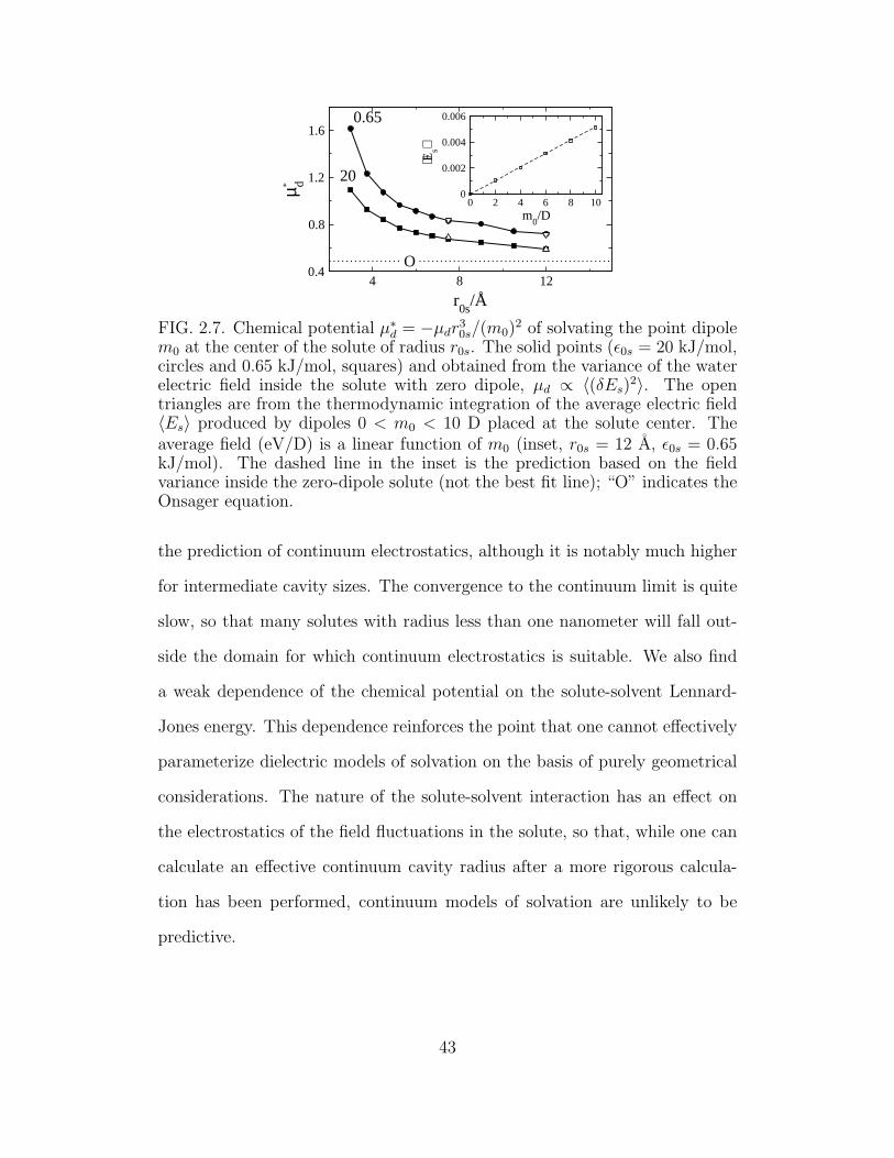
4 8 12

r0s

/Å

0.4

0.8

1.2

1.6

µ d*

0 2 4 6 8 10m

0/D

0

0.002

0.004

0.006

⟨Es⟩

20

0.65

O

FIG. 2.7. Chemical potential µ∗

d = −µdr30s/(m0)

2 of solvating the point dipolem0 at the center of the solute of radius r0s. The solid points (ǫ0s = 20 kJ/mol,circles and 0.65 kJ/mol, squares) and obtained from the variance of the waterelectric field inside the solute with zero dipole, µd ∝ 〈(δEs)

2〉. The opentriangles are from the thermodynamic integration of the average electric field〈Es〉 produced by dipoles 0 < m0 < 10 D placed at the solute center. Theaverage field (eV/D) is a linear function of m0 (inset, r0s = 12 A, ǫ0s = 0.65kJ/mol). The dashed line in the inset is the prediction based on the fieldvariance inside the zero-dipole solute (not the best fit line); “O” indicates theOnsager equation.

the prediction of continuum electrostatics, although it is notably much higher

for intermediate cavity sizes. The convergence to the continuum limit is quite

slow, so that many solutes with radius less than one nanometer will fall out-

side the domain for which continuum electrostatics is suitable. We also find

a weak dependence of the chemical potential on the solute-solvent Lennard-

Jones energy. This dependence reinforces the point that one cannot effectively

parameterize dielectric models of solvation on the basis of purely geometrical

considerations. The nature of the solute-solvent interaction has an effect on

the electrostatics of the field fluctuations in the solute, so that, while one can

calculate an effective continuum cavity radius after a more rigorous calcula-

tion has been performed, continuum models of solvation are unlikely to be

predictive.

43

To verify the effectiveness of the linear response approximation, we per-

formed thermodynamic integration for solutes with r0s equal to 7.5 A and 12

A. Within linear response, the electric field inside the cavity should grow lin-

early in response to the dipole strength in the cavity. Indeed, we find that this

is the case, for dipoles up to 10 Debye. However, as will be shown later, for

cases when the electric field is probed nearer the interface, linear response in

fact breaks down.

Interestingly, while the strength of the Lennard-Jones energy effects the

chemical potential µd, the effect is small, compared to the effect of changing

the solute radius, r0s. Because the two LJ energies used are at the extremes

of intermolecular interactions, the region between the two curves in figure 2.7

may in fact define a region inside which most systems of practical interest in

chemistry will fall. Deviation from this region will likely be an indication of

nonlinear solvation, in which local solvent structure becomes important to the

thermodynamics.

VI Discussion

Addressing the questions posed at the front of this chapter, we have found

(i) a large excess polarization in the water near the solute-solvent interface.

From the studies of dynamics, we find (ii) that at certain interfaces, the dipolar

dynamics can become significantly slowed, compared to bulk water, and that

the slower dynamics can also be seen in the electric field produced by first

shell waters. Addressing the question of length scales (iii), we find that the

dynamical and structural perturbations are significant for hydrations layers

with thickness up to approximately 1 nm. We also find (iv) that the slowed

dynamics of surface waters are not recorded by the Stokes shift dynamics of

44

a dipolar probe placed at the solute center. We also confirm that (v) the

Onsager result for dipole solvation is approached from above, with increasing

cavity radius, and that convergence to this limit is slow.

Given that the polarity scales with the water density, we are able to suggest

a link between the wettability of a solute and the polarity of the hydration

layer. We also note that the dependence of the water dynamics on the surface

composition can lead to the existence of slow and fast domains on a heteroge-

neous surface[72]. However, we also point out that this sort of heterogeneity

will not necessarily be picked up by Stokes shift dynamics, and there is a need

for experiments that are more sensitive to the local hydration dynamics.

45

Chapter 3

NON-GAUSSIAN STATISTICS OF ELECTRIC FIELD FLUCTUATIONS

AT THE SOLUTE-WATER INTERFACE

I Introduction

As discussed in chapter 1, the electric field produced by the solvent inside a

solute is a fluctuating variable. For the case when no external field is applied,

we will denote this field as R. If this field is probed at a dipole m0 placed

on the solute, the average value of R at the dipole is called the reaction

field, R0 = 〈R〉. In this chapter, we aim to understand the statistics of R

produced by water at the interface with a non-polar solute. We introduce a

point dipole close to the solute water interface and study the statistics of R as

the dipole magnitude is increased. Our focus is on the projection of the field

on the direction of the dipole m0; accordingly, we introduce the coordinate

R = m0 · R. The reversible work required for a fluctuation of R away from

its equilibrium value is described by the Landau functional[87] F (R) and the

associated distribution:

p(R) ∝ e−βF (R) ∝

∫

δ (R−R(Γ)) e−βH0dΓ, (3.1)

where H0 is the total system Hamiltonian. The functional F (R) represents

the free energy surface of electric field fluctuations in the absence of a per-

turbation from the solute dipole (i.e., m0 → 0). Within the linear response

approximation, the statistics of R are expected to be Gaussian, and the free

46

energy surface is parabolic with response function κ:

F (R) = R2/(2κ). (3.2)

Introduction of the point dipole modifies the free energy surface to

F(m0, R) = −m0R + F (R). (3.3)

The result, within linear response, is that the shape of the distribution p(R)

is not modified, but only shifted by the amount κm0 (see chapter 1 for a more

detailed discussion).

However, one can imagine that for some situations of interest the shape of

F (R) might be significantly non-parabolic. Consider the solvent response to

an increasing solute dipole. As the field from the solute increases, frustration

is built up in the water hydrogen bond network as the water dipoles align

increasingly with the field. Under strong enough fields, the frustration could

be released, with the water landing in a new state. This new state would

be expected to be harmonic, but around a different (non-zero) minimum, R1

(figure 3.1).

If the scenario described above were realized, several predictions could be

made about the expected resulting observations. If the structure of water

lands in a new state, the curvature of the free energy surface in that state

would likely be different from that in the ground state. The width of thermal

fluctuations about the minimum R1 would be expected to be different from

those around zero. With changing solute dipole m0, the excited state would

be expected to be reduced in free energy by the amount −m0R1 so that states

normally thermally inaccessible to water could become significantly populated.

At some intermediate values of the solute dipole m0 ≃ F0/R1, one would

47

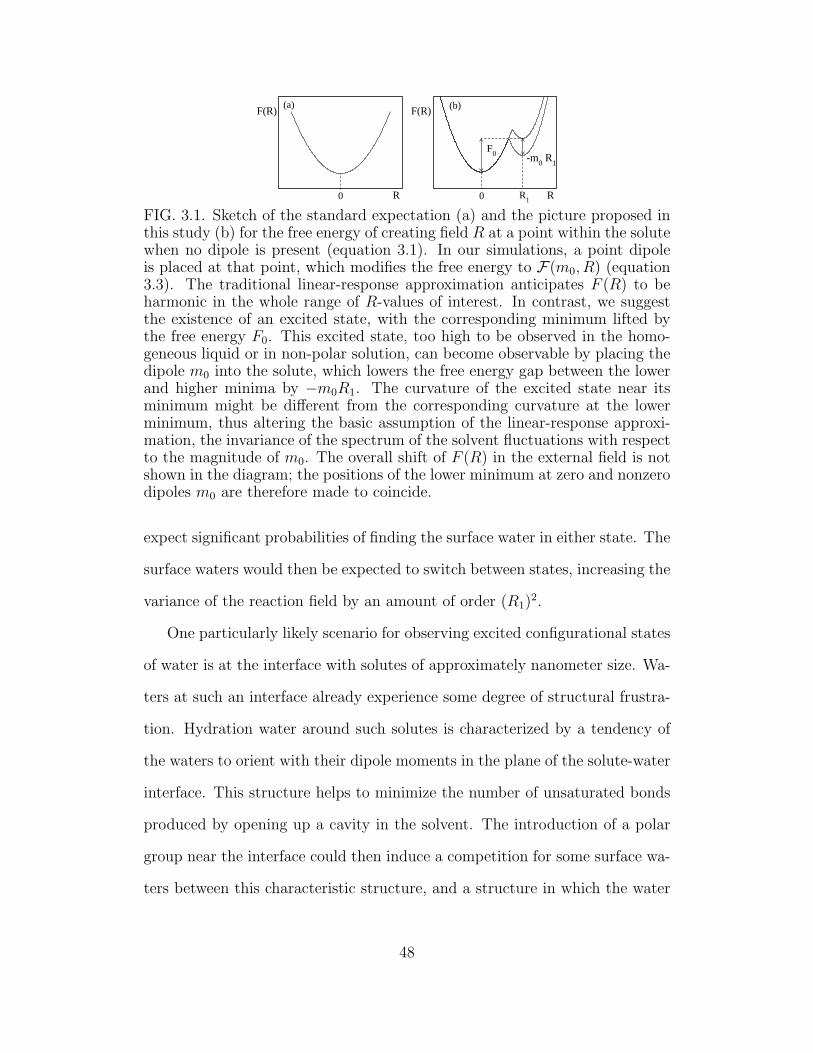
R

F(R)

R

F(R)

0

F0 -m

0 R

1

0 R1

(a) (b)

FIG. 3.1. Sketch of the standard expectation (a) and the picture proposed inthis study (b) for the free energy of creating field R at a point within the solutewhen no dipole is present (equation 3.1). In our simulations, a point dipoleis placed at that point, which modifies the free energy to F(m0, R) (equation3.3). The traditional linear-response approximation anticipates F (R) to beharmonic in the whole range of R-values of interest. In contrast, we suggestthe existence of an excited state, with the corresponding minimum lifted bythe free energy F0. This excited state, too high to be observed in the homo-geneous liquid or in non-polar solution, can become observable by placing thedipole m0 into the solute, which lowers the free energy gap between the lowerand higher minima by −m0R1. The curvature of the excited state near itsminimum might be different from the corresponding curvature at the lowerminimum, thus altering the basic assumption of the linear-response approxi-mation, the invariance of the spectrum of the solvent fluctuations with respectto the magnitude of m0. The overall shift of F (R) in the external field is notshown in the diagram; the positions of the lower minimum at zero and nonzerodipoles m0 are therefore made to coincide.

expect significant probabilities of finding the surface water in either state. The

surface waters would then be expected to switch between states, increasing the

variance of the reaction field by an amount of order (R1)2.

One particularly likely scenario for observing excited configurational states

of water is at the interface with solutes of approximately nanometer size. Wa-

ters at such an interface already experience some degree of structural frustra-

tion. Hydration water around such solutes is characterized by a tendency of

the waters to orient with their dipole moments in the plane of the solute-water

interface. This structure helps to minimize the number of unsaturated bonds

produced by opening up a cavity in the solvent. The introduction of a polar

group near the interface could then induce a competition for some surface wa-

ters between this characteristic structure, and a structure in which the water

48

dipole is flipped to coordinate with the solute dipole. The existence of multiple

orientational states of interfacial water has in fact been demonstrated already

[88, 36, 35]. What has been missing to this point is a study of the ability of

water to switch discontinuously between different states, and the effect of such

a switching on the thermodynamics of solvation. The primary finding of the

present study is the existence of such a crossover and the implications for the

electrostatics of hydration.

II System

In the present work, we use molecular dynamics (MD) simulations of a

nonpolar solute hydrated in SPC/E water. The interactions of the solute with

water oxygen are given again by the Kihara potential:

φ0s(r) = 4ǫ0s

[

(

σ0s

r − rHS

)12

−

(

σ0s

r − rHS

)6]

. (3.4)

We then introduce a point dipole, oriented along the radial direction and

located a distance rd from the solute center (see figure 3.2). We study dipoles

up to 10 Debye in magnitude, and situated at two distances, rd = 9 A and rd =

10 A from the solute center. Further simulation details are given in Appendix

B.

We study the change in the spectrum of fluctuations of the water electric

field R, measured at the solute dipole, as the solute dipole moment is increased.

Figure 3.3 shows the dependence of the reaction field R on the solute dipole.

The top panel in figure 3.3 shows the results for rd = 10 A, and the bottom

panel shows the data for rd = 9 A. For small magnitudes of the solute dipole,

the prediction of linear response is followed, and the reaction field scales with

the dipole moment. But as the dipole moment is increased further, a crossover

49

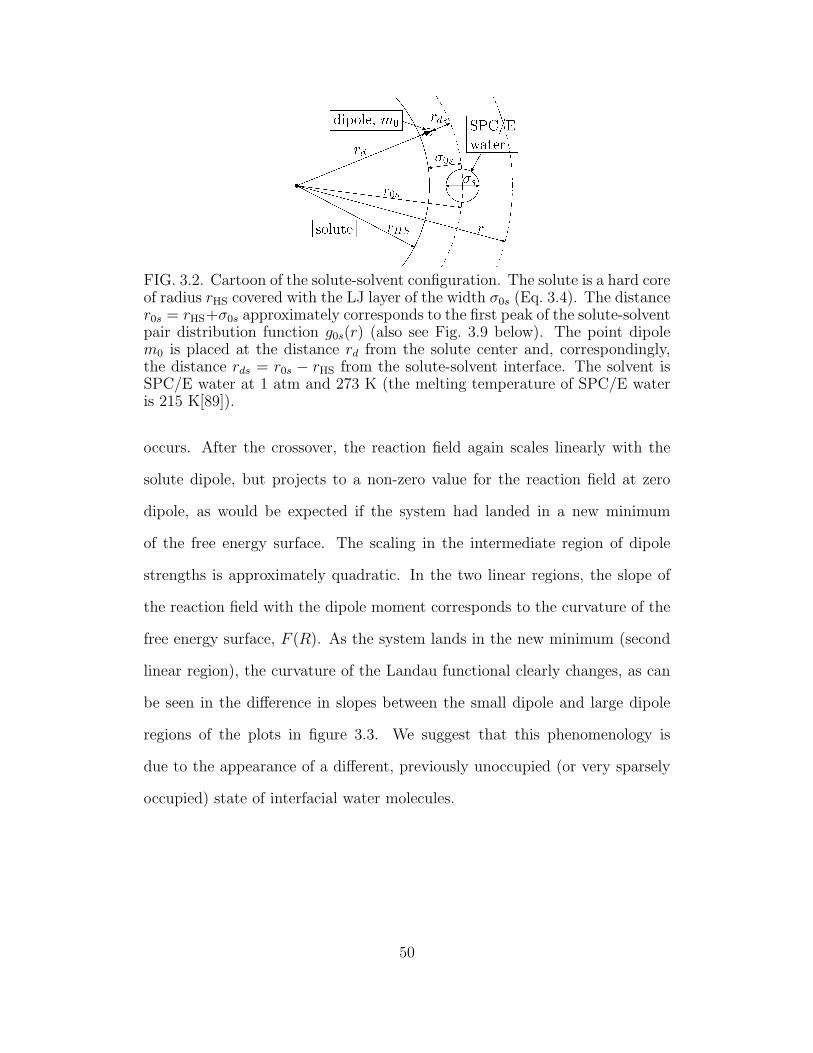
FIG. 3.2. Cartoon of the solute-solvent configuration. The solute is a hard coreof radius rHS covered with the LJ layer of the width σ0s (Eq. 3.4). The distancer0s = rHS+σ0s approximately corresponds to the first peak of the solute-solventpair distribution function g0s(r) (also see Fig. 3.9 below). The point dipolem0 is placed at the distance rd from the solute center and, correspondingly,the distance rds = r0s − rHS from the solute-solvent interface. The solvent isSPC/E water at 1 atm and 273 K (the melting temperature of SPC/E wateris 215 K[89]).

occurs. After the crossover, the reaction field again scales linearly with the

solute dipole, but projects to a non-zero value for the reaction field at zero

dipole, as would be expected if the system had landed in a new minimum

of the free energy surface. The scaling in the intermediate region of dipole

strengths is approximately quadratic. In the two linear regions, the slope of

the reaction field with the dipole moment corresponds to the curvature of the

free energy surface, F (R). As the system lands in the new minimum (second

linear region), the curvature of the Landau functional clearly changes, as can

be seen in the difference in slopes between the small dipole and large dipole

regions of the plots in figure 3.3. We suggest that this phenomenology is

due to the appearance of a different, previously unoccupied (or very sparsely

occupied) state of interfacial water molecules.

50

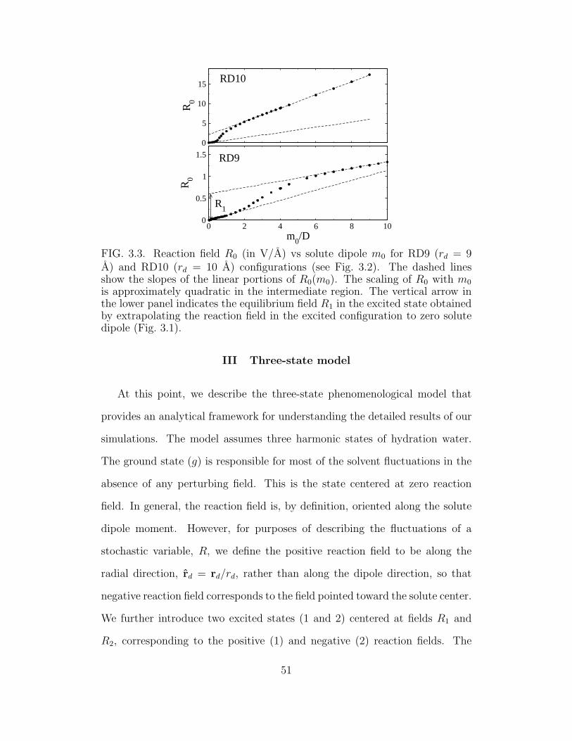
0

5

10

15

R0

0 2 4 6 8 10m

0/D

0

0.5

1

1.5

R0

RD10

RD9

R1

FIG. 3.3. Reaction field R0 (in V/A) vs solute dipole m0 for RD9 (rd = 9A) and RD10 (rd = 10 A) configurations (see Fig. 3.2). The dashed linesshow the slopes of the linear portions of R0(m0). The scaling of R0 with m0

is approximately quadratic in the intermediate region. The vertical arrow inthe lower panel indicates the equilibrium field R1 in the excited state obtainedby extrapolating the reaction field in the excited configuration to zero solutedipole (Fig. 3.1).

III Three-state model

At this point, we describe the three-state phenomenological model that

provides an analytical framework for understanding the detailed results of our

simulations. The model assumes three harmonic states of hydration water.

The ground state (g) is responsible for most of the solvent fluctuations in the

absence of any perturbing field. This is the state centered at zero reaction

field. In general, the reaction field is, by definition, oriented along the solute

dipole moment. However, for purposes of describing the fluctuations of a

stochastic variable, R, we define the positive reaction field to be along the

radial direction, rd = rd/rd, rather than along the dipole direction, so that

negative reaction field corresponds to the field pointed toward the solute center.

We further introduce two excited states (1 and 2) centered at fields R1 and

R2, corresponding to the positive (1) and negative (2) reaction fields. The

51

solvent response in each state, g, 1, 2, is characterized respectively by κα, with

α = g, 1, 2. The response functions κα have dimensions of inverse volume;

we can then define the length scale, ℓαR = κ−1/3α . This length scale reflects the

depth at which the a dipolar probe placed in the solute will be affected by

the solvent fluctuations. We introduce three states, rather than just the two

described in the introduction, in order to reflect the possibility of the surface

dipoles flipping to orient either along or against the radial direction (see figure

3.4). The minima of the two states are lifted by the free energies F1 and F2

above the ground state.

The introduction of the solute dipole modifies the free energy surfaces in

each of the three states, by lowering the free energy by the amount, −m0R.

The free energies of the three states (g, 1, 2) are then given by:

Fα(m0, R) = Fα(R)−m0R. (3.5)

The total free energy surface describing the reaction field fluctuations is then

given by the trace over the states available to the system:

e−βF(m0,R) =∑

α

e−βFα(m0,R). (3.6)

As with our previous simulations of Kihara solutes with no perturbing dipole,

we calculated the first and second orientational parameters, pI1 and pI2, of the

waters in the first hydration shell:

pI1 = (N I)−1∑

j=1,NI

mj · rj, (3.7)

and

pI2 = (2N I)−1∑

j=1,NI

[

3(mj · rj)2 − 1

]

. (3.8)

The results for the first orientational parameter are shown in panel A of figure

3.5. The value of pI1 is close to zero, indicating almost no asymmetry in

52

!2

!g

!1

F0

0 R1

FIG. 3.4. Illustration of the phenomenological model we use to understand ourresults. The surface F (R) is a superposition of a ground state and two excitedstates lifted above the ground state by the free energy F1 (top panel). Thebottom panel shows a cartoon of the two scenarios for the excited state. Awater molecule breaks free from the hydrogen bond network and coordinateswith the field from the solute.

53

the orientation of the hydration waters, corresponding to approximately zero

electric field inside the cavity at zero solute dipole. The second orientational

parameter, however, is significantly negative, indicating a tendency for the

water dipoles to orient in the plane of the interface.

0 2 4 6 8 10m

0/D

-0.2

-0.18

-0.16

-0.14p 2I

RD10RD9

0 2 4 6 8 100.032

0.036

0.04

FIG. 3.5. Second [pI2, Eq. (3.8)] (main panel) and first [pI1, Eq. (3.7)] (inset)orientational order parameters for RD9 (rd = 9 A, filled squares) and RD10(rd = 10 A, open squares) configurations.

These results, along with the observation that 〈R〉 ≃ 0 when m0 → 0, indi-

cate that there is little asymmetry in the distribution of thermally accessible

configurations of the interfacial dipoles at m0 → 0, due to the low popula-

tions of the excited states. Our data for positive m0 are not very sensitive to

the values of R2 and F2. As a result, adequate numerical fits of the simula-

tion data are produced with a reduced set of model parameters: R1 = −R2,

54

F1 = F2 = F0 and κ1 = κ21. The free energies of the three states then become

Fg(R) =R2/(2κg),

F1(R) =(R−R1)2/(2κ1) + F0,

F2(R) =(R +R1)2/(2κ1) + F0.

(3.9)

Four model parameters κg, κ1, R1, and F0 were fitted to the field variance

σ2R(m0) from MD data (see figure 3.7a). They are listed in Table 3.1 and

are used to produce plots of R0(m0), σ2R(m0), and F(m0, R) presented in the

Results section below.

Table 3.1. List of model parameters produced by fitting the three-state modelto σ2

R(m0) from MD simulations. ℓαR = (κα)−1/3, α = g, 1 is the characteristic

length of penetration of water’s surface fluctuations into the solute.

Configuration rd, A βF0 ℓgR, A ℓ1R, A R1, V/A

RD9 9 7.3 3.0 3.1 0.3

RD10 10 7.2 1.5 1.2 1.0

IV Results

All the simulation results that we discuss below have been produced for

two distances between the point dipole in the solute and its center (Fig. 3.2),

1Because of the asymmetry of water’s molecular charge, the free energy surface F(0, R)

is in principle asymmetric with respect to the transformation R → −R. Excitations to the

R2 state probably require less free energy, F2 < F1, since less stringent rearrangement of

the hydrogen bond network is required. This problem warrants further studies, in particular

in applications to surfaces with alternating charges, such as those of proteins. Our present

results, restricted to solute dipoles parallel to the radial direction rd do not show significant

deviations from the assumed symmetric behavior, although fits to the model might improve

if this requirement is lifted at the expense of a larger number of fitting parameters.

55

rd = 9 A and rd = 10 A. We will reference them below as states RD9 and

RD10, respectively.

As noted above, the dependence of the reaction field R on the solute dipole

m0 is characterized by two linear regions, with a fairly broad crossover region,

which is the signature of the transition between the lower (ground) and the

higher free-energy states of the solvent. The two states are clearly distin-

guished in the changes in the free energy surfaces of reaction field fluctuations,

as the solute dipole is increased. Figure 3.6 shows the free energy surfaces for

the RD10 state for several solute dipoles, as the system passes through the

crossover. Initially, the surface is single-welled, although it should be noted

that the wings of the curve are almost flat, rather than parabolic. For slightly

larger values of m0, a shoulder appears at higher values of R. As the solute

dipole is increased further, the surface becomes double-welled; at still higher

dipole moments, the surface water moves completely into the excited state,

and the free energy surface returns to a single-welled shape. The overall be-

havior is reminiscent of the phenomenology of a first order phase transition;

however, it should be noted that the observations reported here seem to cor-

respond to a fairly localized change in the solvent structure, involving just a

few water molecules (see below).

The phenomenology of first order phase transitions generally predicts that

far from the transition point, fluctuations will be Gaussian. As the transition

point is approached, the statistics of fluctuations are expected to become sig-

nificantly non-Gaussian, with a maximum in the fluctuations occurring near

the transition point[90]. For example, in the case of a temperature-controlled

transition, one expects a spike in the heat capacity. As expected, our results

show a peak in the variance of the reaction field, σ2R = 〈(δR)2〉, when the

56

-2 0 2 4

-8

-4

0

βF(R

)

-2 0 2 4

-8

-4

0

-2 0 2 4

-8

-4

0βF

(R)

-2 0 2 4

-8

-4

0

-2 0 2 4R

-8

-4

0

βF(R

)

-2 0 2 4R

-8

-4

0

0.2 D 0.3 D

0.5 D 0.6 D

0.7 D 0.8 D

FIG. 3.6. Free energies F(m0, R) (equation 3.3) for the RD10 state (rd = 10A) at m0 values indicated in the plots. The electric field at the solute dipolein the abscissa is in V/A; the dashed lines refer to the fits to the three-statemodel (equations 3.5 and 3.6). The model parameters used in the plot arelisted in Table 3.1. For reference, 1 Debye in the RD10 state corresponds to areduced dipole m∗ = 3.0 (see equation 3.10 below).

system passes through the transition, as shown in figure 3.7. The results are

plotted against a reduced dipole moment that reflects approximately the ratio

of fields produced by the solute and by neighboring water molecules at the

solute-water interface:

m∗

0 =m0

ms

(

σs

rds

)3

, (3.10)

where ms and σs are the solvent (water) dipole moment and diameter, respec-

tively, and rds = r0s − rHS is the distance from the dipole to the solute-water

57

interface. Similar ideas are used to introduce the reduced instantaneous field:

R∗ = Rr3ds/ms. (3.11)

Its average, R∗

0, and variance, 〈(δR∗)2〉, are shown in Fig. 3.7.

0

2

4

R0*

0

0.1

0.2

⟨(δR

*)2

⟩

RD9RD10

0 2 4 6 8 10

m0

*

0

0.5

1

τ eff/p

s RD9RD10

(a)

(b)

(c)

Na+

Na+

Na+

--OH

--OH

--OH

FIG. 3.7. The average, R∗

0, of the reduced field R∗ as defined by Eq. (3.11)(a) and its variance (b) vs the reduced solute dipole defined by Eq. (3.10).The filled squares and solid lines in (a) and (b) refer, respectively, to the MDresults and their fit to the three-state model for the RD9 configuration; theopen squares and the dashed lines carry the same information for the RD10configuration. Panel (c) shows the relaxation time τeff of the water field self-correlation function (see text) obtained from MD simulations for RD9 (solidline) and RD10 (dashed line) configurations. The dotted vertical line showsthe approximate field generated by the hydroxyl of aqueous methanol at thenearest water oxygen, and the dash-dotted vertical line corresponds to thesame quantity for sodium ion in water.

58

In order to provide context for these results, we estimated the field strengths

produced by sodium ion and by the hydroxyl of aqueous methanol at the near-

est water oxygen. The solute-water distances required for this estimate are

taken from corresponding distribution functions from references [19] and [91].

The vertical lines in figure 3.7 are drawn at the values of m∗

0 that reflect the

fields from these solutes, normalized in the same way as m∗

0 and R∗. The field

of a hydroxyl falls in the range that is expected to produce significant popula-

tions of both water states. In contrast, the much stronger field of the sodium

cation is sufficient to push the interfacial water predominantly into the excited

state.

To study the dynamics associated with the crossover, we calculated the

time self-correlation function, S(t) = 〈δR(t)δR(0)〉/〈(δR)2〉. We fit the re-

laxation function to a sum of exponentials; one can then define an average

relaxation time, τeff =∫

∞

0dtS(t). This relaxation time passes through a maxi-

mum in the same range as the spike in the field variance, similar to the critical

slowing associated with first order phase transitions[92, 93].

The degree of deviation from Gaussian statistics can be quantified by the

parameter χG = m0β〈(δR)2〉/〈R〉, the temperature-reduced ratio of the vari-

ance of the solute-water energy to its average, equal to 1 when the linear

response approximation is valid. This parameter is plotted for increasing so-

lute dipole in figure 3.8. Not surprisingly, we see a spike in this parameter in

the area of the transition. In order to elucidate the extent of the deviation

from linear response, we show in figure 3.6 the direct calculation of the reac-

tion field factor, κ from the ratio of the reaction field to the solute dipole; that

is, κ = R0/m0. We compare this to the prediction of linear response, calcu-

lated from fluctuations in the cavity: κ = βσ2R. Again, since in linear response

59

this variance is independent of the solute dipole, the horizontal dashed line in

figure 3.6 reflects the value to which both these quantities converge if linear

response is applicable.

0 2 4 6

m0

*

0

50

100

150

(r0s

/l R)3

LRAcontinuum

0 2 4 60

1

2

3

χ G

RD10RD9

(a)

(b)

FIG. 3.8. Comparison of results with the predictions of linear response andof continuum electrostatics. In panel (a), we show the Nonlinearity parameterχG (equation 1.15) obtained from MD simulations (points) and from fittingthe three-state model (lines). Panel (b) shows the reduced stiffness parameterκr30s = (r0s/ℓR)

3 calculated in different approximations for RD9. The dash-dotted line, κ = R0/m0, is from the dielectric continuum calculation for thereaction field at a dipole inside a dielectric cavity (Eq. 3.12). The dashedline shows κ = βσ2

R obtained from the variance σ2R at m0 = 0. The open

circles show κ = R0/m0 and open squares refer to κ = βσ2R, both from MD

simulations. In linear response, circles and squares are expected to collapse onthe dashed line (Eq. 1.12).

To give further context to these results, we also indicate the value obtained

for κ if the solute is modeled as a point dipole placed inside a cavity (ǫ = 1)

in a continuum dielectric. The reaction field in this approximation is given, to

a very good approximation, by:

R0 =m0

r30s

ǫ− 1

2ǫ+ 1

(

2−z2

ǫ+ 1

)

1 + z2

(1− z2)3, (3.12)

60

where z = rd/r0s. The derivation of this result is given in Appendix D. The

continuum cavity radius in this calculation was chosen at r0s = 11.5 A, slightly

below the position of the first peak of the solute-solvent pair distribution func-

tion at ≃ 12 A(Fig. 3.9). This value was chosen for a number of reasons, given

in Appendix D. Most importantly, however, this value for the continuum ra-

dius produces the proper scaling of the reaction field with the dipole-interface

distance: R ∼ r−30s . The choice of a value that produces this scaling allowed the

collapse of the data in figure 3.3; when this value is used for the continuum

cavity radius, the solvent response approaches the prediction of continuum

electrostatics for large dipoles.

12 14 16

r/Å

0

1

2

3

4

5

g 0s(r

)

1 D

4 D

6 D

9 D

FIG. 3.9. Solute-oxygen pair correlation function for RD9, inside the solidangle defined in the text (also see Appendix E). The numbers in the plotindicate values of the dipole moment m0. The curves are shifted vertically by1.0 for a better view.

Having drawn the comparison of the observed phenomenology to that of

phase transitions, the question naturally arises of what is the nature of the

structural change associated with the excited state of the surface water. Specif-

ically, one wonders what is the spacial extent of the structural perturbation.

Our results presented above for the orientational parameters of the surface

waters seem to imply that the transition is relatively localized. If a structural

61

change were propagating over a significant portion of the interface, one would

expect a significant effect on the orientational structure of the surface water.

To address this question more directly, we examine the water structure

within a solid angle of 54.8 (see Appendix E for a drawing). This region

includes all surface waters within an arc length of 2σw from the dipole axis.

The pair correlation function of the dipole with water oxygen was calculated

for waters lying inside this solid angle. As the solute dipole is increased, a

new peak emerges from the first hydration layer. Integration of this peak

indicates that exactly one water molecule breaks free from the hydrogen bond

network and shifts toward the solute. One expects that some level of strain

is introduced in the neighboring molecules. The picture one arrives at is that

two hydrogen bonds are broken, and the water oxygen, freed from the network,

rotates and coordinates to the solute. This picture is supported by the value

we obtained for the excitation free energy, F0 ≃ 7 kBT , which is approximately

the enthalpy required to break two hydrogen bonds in SPC/E water[94].

The strain in the hydrogen bond network associated with the excitation

is evident in the distribution of O-O-H angles between neighboring first shell

water molecules inside the same solid angle. To define the hydrogen bond

angle, we first take the line through the two oxygen nuclei; then, of the four

associated hydrogen atoms, we choose the O-H bond that makes the small-

est angle with the O-O line (see figure 3.10, inset). These distributions are

shown for three different dipole moments in figure 3.10. The occupation of

the buckled state with the larger hydrogen bond angle grows with increasing

solute dipole moment. The definition used here for the hydrogen bond angle is

borrowed from the work of Kim Sharp[88]. Similar distributions of hydrogen

bond angles at interfaces of varying charge were seen by Sharp and cowork-

62

ers. However, that work so far only showed that the distribution becomes

bimodal at charged interfaces, and the present study adds to this the finding

that water can be made to switch between the different states, with significant

implications for the hydration thermodynamics. In fact, it is a quite general

property of water at interfaces that the electric fields from the solutes cause

the water molecules to repopulate different states without significant changes

to the states themselves[35]. A similar phenomenology has also been found in

numerical simulations of a planar surface in contact with water, with a gradual

increase in surface polarity[36].

FIG. 3.10. Distributions of O-H-O angles θ for the RD10 configuration at m0

equal to 0.01, 3.5, and 10 D. The distributions were calculated according to thealgorithm suggested by Sharp et al [88] in the region of the first hydration layerwithin the solid angle cutting the circumference length of 2σs at the surface(see Appendix E). The inset shows the definition of the bond angle and thedistance cutoff within which the angles were sampled.

V Discussion

We have presented here a study of the statistics of the electric field pro-

duced by hydration water inside a nanometer-sized solute. We find that these

statistics are significantly altered when a dipole is placed on the solute, near

the interface. As the dipole magnitude is increased, the surface waters respond

by populating an excited state, which is higher in free energy than the ground

state by approximately the energy needed to break two hydrogen bonds (≃ 7

63

kBT ). The excited state is characterized by a domain of surface waters with

a distorted hydrogen bond network. To put the water into the excited state,

what is required is the field of a dipole approximately twice water’s, located

approximately one solvent diameter from the water closest approach radius.

The electric field strength produced by this dipole at the interface puts the

system at a crossover point with the system jumping between the two states,

and characterized by strongly non-Gaussian fluctuations.

Because of the local nature of the excitations associated with this transi-

tion, the area characterized by the fluctuations in excess of linear response is

actually quite broad, with significant populations of both states present for a

range of solute dipoles. This is in contrast to what one observes for a bulk

phase transition, which is characterized by global changes, strongly localized

in thermodynamic parameter space. Accordingly, significant populations of

the excited state could be reached with weaker perturbations, such as a hy-

droxyl or other polar functional group. The fields from small monatomic ions

are expected to be strong enough to switch surface waters completely into the

excited state.

The phenomena described here should be observable by optical probes.

A probe near a water domain that predominantly exists in one state will

record a spectral shift and spectral width that are proportional to the change

in dipole moment of the probe and related by the general results of linear

response. In contrast, a probe placed near a domain of water that is near the

coexistence point of the two states will record a distinctly broadened spectral

width, and an altered spectral shift. If good measurements of spectral widths

can be performed, it should be possible to observe the breakdown of linear

response for such a system. It should also be noted that the way in which this

64

transition manifests itself will depend on where the two electronic states lie on

the plots in figure 3.7. If the two electronic states lie on opposite sides of the

transition, an enhanced spectral shift will be observed, with a small change

in the width. In contrast, any electronic state producing a domain of water

close to the coexistence point will be characterized by a significantly broadened

spectral line. In the case of real optical probes, the interface will likely present

a mosaic of water domains in different states. For that reason, experiments

could usefully be analyzed in terms of the ideas developed here, but results may

be best understood as probing average properties of the hydration water. It

should also be noted that without a large number of data points, the deviations

from the predictions of simple linear solvation models will be difficult to detect

by measurements of spectral shift, since if one has only a few points, the ‘S’

shape of the solvent response will likely appear as a line with some level of

noise. The spectral width is therefore a much better probe of the local solvent

structure than the spectral shift.

Our results also predict that Stokes shift dynamics will slow down when

water is near the transition region, as seen in figure 3.7c. A nanoscale solute

decorated by a mosaic of charges will then produce a dynamically heteroge-

neous Stokes shift response[72]. The dynamics observed here are still much

faster (ps) than the slow dynamics observed in Stokes shift experiments on

chromophores bound to proteins (ns) [95, 50, 96]. The difference of three or-

ders of magnitude between the two suggests the possibility that the chemically

heterogeneous surfaces of proteins can produce cooperative domains of several

excitations. Alternatively, it can also be argued that all the slow dynamics of

water at the protein-water interface are due to coupling of the water to protein

65

motions[51]. And it is of course possible that the overall response of biological

water is best described as a combination of these effects[97].

66

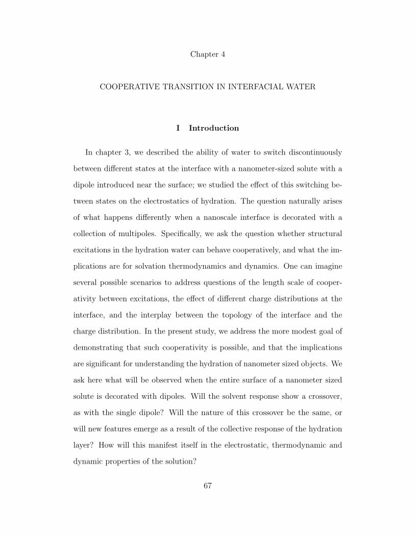
Chapter 4

COOPERATIVE TRANSITION IN INTERFACIAL WATER

I Introduction

In chapter 3, we described the ability of water to switch discontinuously

between different states at the interface with a nanometer-sized solute with a

dipole introduced near the surface; we studied the effect of this switching be-

tween states on the electrostatics of hydration. The question naturally arises

of what happens differently when a nanoscale interface is decorated with a

collection of multipoles. Specifically, we ask the question whether structural

excitations in the hydration water can behave cooperatively, and what the im-

plications are for solvation thermodynamics and dynamics. One can imagine

several possible scenarios to address questions of the length scale of cooper-

ativity between excitations, the effect of different charge distributions at the

interface, and the interplay between the topology of the interface and the

charge distribution. In the present study, we address the more modest goal of

demonstrating that such cooperativity is possible, and that the implications

are significant for understanding the hydration of nanometer sized objects. We

ask here what will be observed when the entire surface of a nanometer sized

solute is decorated with dipoles. Will the solvent response show a crossover,

as with the single dipole? Will the nature of this crossover be the same, or

will new features emerge as a result of the collective response of the hydration

layer? How will this manifest itself in the electrostatic, thermodynamic and

dynamic properties of the solution?

67

To study the response of water at a nanoscale interface to a collection of

perturbing dipoles, we study a system having the geometry of C180 fullerene.

We introduce point dipoles on each carbon atom, oriented so that the dipole

moment direction is along the radius vector (the vector from the center of mass

of the fullerene to the carbon atom). We simulated this system by molecular

dynamics using the NAMD 2 package [98] with 37924 hydration waters. Water

was represented by the SPC/E model [75]. For the Lennard-Jones interactions

of the fullerene carbon with water oxygen, the AMBER atom type CA[99] was

used, with the Lennard-Jones radius given by the arithmetic combination rule,

and the Lennard-Jones well depth given by the geometric combination rule.

We simulated systems with the carbon dipole magnitude ranging between 0.5

Debye and 9.0 Debye. Following 10 ns equilibration, we simulated each system

for 40 ns at 310 Kelvin. Further simulation details are given in Appendix G.

II Results

We first examine the dependence of the solute-solvent electrostatic energy,

u0s on the strength of the dipole moment,mC . This quantity is easy to compare

to the results from the Kihara solute with single dipole, presented in chapter

3. We define the reduced solute-solvent energy, scaled to reflect the magnitude

of the electrostatic energy between the carbon dipole and the surface water

dipoles:

u∗

0s = u0s ×r3Cs

mCms

, (4.1)

where u0s is the total electrostatic solute-solvent energy, mC is the magnitude

of the dipole moment placed on the carbon atoms, ms is the dipole moment

of SPC/E water, 2.351 D, and rCs is the distance from the carbon dipoles to

the interface. In accordance with the estimate of the continuum radius in our

68

work on the Kihara solutes in chapter 3, we use the value, rCs = σCO − 0.5A

= 2.86 A, where σCO is the Lennard-Jones diameter for fullerene carbon in-

teracting with SPC/E oxygen. We present the average and variance of u∗

0s in

figure 4.1; the solid squares represent the results from the present study of

C180; we scale these by the factor 1/180, in order to compare to the results

for the Kihara solute. The x-axis in figure 4.1 is the reduced dipole moment,

m∗ = (mC/ms) × (σs/rCs)3. The hollow squares and hollow circles show the

results of the Kihara plus dipole study, with rd = 9 A and rd = 10 A, respec-

tively. The results for the C180 solute follow the behavior seen for the Kihara

study, for small magnitudes of mC . This is consistent with the picture that

individual structural excitations in the solvent are uncorrelated, so that the

average behavior reflects the behavior seen for a single perturbation. However,

as the perturbing dipoles are increased further, a second peak emerges in the

variance. This second broad peak seems to correspond to the emergence of

cooperative switching between states in the hydration shell.

In figure 4.2, we also show the result for the non-Gaussianity parameter,

χG = −β〈(δu0s)2〉/〈u0s〉. This parameter goes through two distinct peaks.

The indication is that the fluctuations are in excess of the expectations of

linear response for a very broad range of surface polarity.

To understand the physical origin of these observations, we examine the

first and second orientational parameters of the surface waters. We consider

waters with the center of mass at distances less than 8.5 A from the solute

center. We define the order parameters as in chapters 2 and 3; the results

are presented in figure 4.3. The first orientational parameter, indicated by

the open circles, is small and positive for small mC . With increasing dipole

moment, pI1 decreases in two features, until ending at pI1 ≈ −0.25. We also find

69

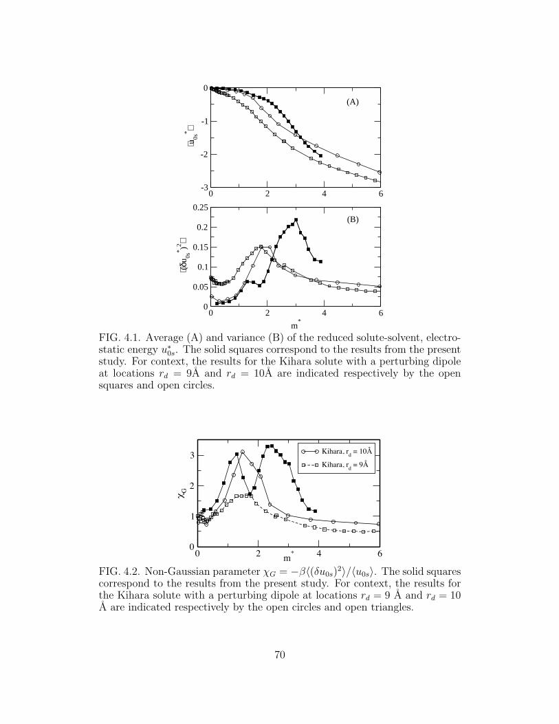
0 2 4 6-3

-2

-1

0

⟨u0s

* ⟩

0 2 4 6

m*

0

0.05

0.1

0.15

0.2

0.25

⟨(δu

0s

* )2 ⟩

(A)

(B)

FIG. 4.1. Average (A) and variance (B) of the reduced solute-solvent, electro-static energy u∗

0s. The solid squares correspond to the results from the presentstudy. For context, the results for the Kihara solute with a perturbing dipoleat locations rd = 9A and rd = 10A are indicated respectively by the opensquares and open circles.

0 2 4 6m*

0

1

2

3

rG

Kihara, rd = 10Å

Kihara, rd = 9Å

FIG. 4.2. Non-Gaussian parameter χG = −β〈(δu0s)2〉/〈u0s〉. The solid squares

correspond to the results from the present study. For context, the results forthe Kihara solute with a perturbing dipole at locations rd = 9 A and rd = 10A are indicated respectively by the open circles and open triangles.

70

0 1 2 3 4

m*

-0.2

-0.1

0

p 1I , p2I

p2

I

p1

I

FIG. 4.3. First and second orientational order parameters,pI1 and pI2 for thefirst shell waters. The open circles and open squares represent, respectivelythe first and second parameters.

two features in the behavior of the second orientational parameter, pI2 (open

squares in figure 4.3). This parameter starts at a negative value for small mC ,

indicating the preference of waters to orient in the plane. With increasing

mC , pI2 decreases in magnitude with a weak shoulder at mC ≈ 3.5 to 4.0 D

(m∗ ≈ 1.5). as the carbon dipoles increase further, the second orientational

parameter crosses zero and passes through a peak, then levels off at a small,

positive value, indicating a weak preference for orientation of the water dipoles

along the radial direction.

The negative values of pI1 for large solute dipoles indicate surface water

dipoles oriented somewhat against the dipoles placed on the carbon atoms.

This seemingly counterintuitive result is easily understood from the arrange-

ment of water molecules around fullerenes. Greater surface area contact and

more favorable packing are achieved when waters occupy the area near the

centers of the faces of a fullerene[100]. Consequently, in our system, the wa-

ters are sensitive mostly to the equatorial electric field from the carbon dipoles.

As a result, the waters tend to point opposite the dipoles placed on the solute.

The difference observed here, compared with what was found for the Kihara

71

solute with the dipole placed near the surface, highlights the effect the solute

topology can have on the orientational properties of the interfacial waters.

If the second transition observed in this progression is indeed the result

of cooperative rearrangement of the interface waters, one expects to see this

reflected in the dynamics. We consider first the self time correlation function,

C1(t) = 〈(pI1(t)pI1(0)〉, where pI1(t) is the instantaneous value of the order pa-

rameter pI1. We fit the resulting function to a sum of two exponentials. The

faster of the two has a timescale of approximately 0.2 to 0.5 ps, consistent with

the dynamics of bulk SPC/E water [101]. We plot the time constant τE of the

slower exponential in figure 4.4, indicated by the solid squares. The timescale

spikes to the nanosecond range in the vicinity of the second transition, much

like the phenomenology of a first order phase transition; after the spike, the

sudden drop of the relaxation time occurs at higher dipole moments than the

maximum in fluctuations, reminiscent of spinodal decomposition [102, 103].

We also calculated the autocorrelation function for the electrostatic solute-

solvent energy. We analyze the dynamics in the same way, and the results are

shown in figure 4.4 by the open circles. The dynamics of the hydration energy

follow the dynamics of the orientational motion in the hydration layer (figure

4.4).

The transition is accompanied by a change in the water density around

the solute. Waters in the excited state are notably closer to the solute than

those occupying the state with the dipoles oriented in the plane of the solute-

water interface. In figure 4.5, we show the mean number of waters within

8.5 A of the solute center N1, with increasing dipole moment. As the excited

state population increases, the number of waters within this distance cutoff

72

0 2 4

m*

0

500

1000

1500

2000

τ 2/ps

p1

I

u0s

FIG. 4.4. Exponential relaxation time, τ2, of the slow component of the relax-ation of the orientational parameter pI1 (solid squares) and of the electrostaticsolute-solvent energy u0s (open circles).

0 2 4

m*

40

50

60

70

80

90

100

N1

FIG. 4.5. Number of waters with oxygen within 8.5 A of the solute center ofmass. The number increases as the system goes through the crossover, thenlevels off as the excited state is saturated.

increases and as the transition completes, the number of waters in the first

shell saturates.

III Chemical Potential

The solute-solvent interaction energy is an easy quantity to calculate, but

is not directly observable. However, one can determine the chemical potential

73

of electrostatic solvation of the fullerene by thermodynamic integration[13, 14].

µel =

∫ 1

0

dλ

⟨(

∂u0s

∂λ

)⟩

λ

, (4.2)

where µel is the electrostatic chemical potential, u0s is the electrostatic solute-

solvent energy, and λ = m/mC .

For the case of turning on the carbon dipoles, we write the total solute-

solvent electrostatic energy as u0s = −∑

i mi ·Ei = −m∑

i mi ·Ei, where mi

is the dipole moment on the ith carbon, and Ei is the solvent electric field at

the ith carbon. Then for the integration, we get:

µ =

∫ mC

0

dm u0s(m)/m. (4.3)

Within linear response, this gives: [14, 9, 104]

µ = u0s/2 ∝ (mC)2. (4.4)

However, the response we see here is clearly non-linear (see figure 4.1), so that

we calculate the chemical potential here from numerical integration of equation

4.3. We have performed this analysis for our C180 solute, with the results given

in figure 4.6a. We plot the reduced chemical potential, µ∗ = µr3Cs/(mC)2.

Within linear response, this will be constant with changing mC . What we

find is that the chemical potential scales very roughly with m2C only for small

dipoles, up to about 2 D, before increasing in magnitude significantly faster

than m2C . The scaling for larger dipoles is approximately third order in mC ,

as can be seen from the bottom panel, figure 4.6b, which shows the log-log

plot of µ∗ vs. m∗. For large dipole moments, the slope of ln(µ∗) with ln(m∗)

is about 1.5, indicating a scaling of µ ∼ (mC)3.5.

74

0 1 2 3 4

m*

-20

-15

-10

-5

0µ∗

-2 -1 0 1 2

ln(m*)

1

1.5

2

2.5

3

ln(-

µ* )(A)

(B)

Slope = 1.46

FIG. 4.6. Electrostatic chemical potential of the C180 solute calculated fromthermodynamic integration. The top panel (A) shows the reduced chemicalpotential, µ∗ = µr3Cs/m

2C ; this quantity is constant in the case of linear solva-

tion. The x-axis is the reduced dipole, m∗ = (mC/ms)(σs/rCs)3. The bottom

panel (B) shows the log-log plot of µ∗ vs. m∗; the slope gives the scaling of µwith the carbon dipole strength.

75

IV Discussion

The results presented here indicate that the structural excitations induced

in the waters near the interface with a nanometer size object can behave in

a cooperative manner, switching between different collective states. Near the

point of transition, the associated solvation dynamics become quite slow, with

timescales reaching nanoseconds. While the dynamics become cooperative,

the broadness of the transition observed implies that the structural changes

still must still be fairly limited in size. The whole hydration layer does not flip

between states in a concerted manner.

Because of the tendency of interface waters to occupy the faces of the

fullerene, the excited state studied here actually represents the opposite side

of the curve obtained in our previous study of the Kihara solute with a single

point dipole. This confirms that such a state exists and also emphasizes that

the specific structural changes in water at real interfaces will be quite sensitive

to both the charge distribution and the topology.

It was recently suggested that biomolecules place water near the critical

point of the weak dewetting transition associated with hydrophobic solvation

[7]. Our present results indicate the existence of another critical point, between

hydrophobic and hydrophilic hydration of nanometer-sized objects that may

also be important for biology. The fluctuations at a nanoscale interface can

likely be tuned by adjusting the charge density and distribution. This points

to a possible link between protein function and protein structure.

Linear solvation models are expected to fail for hydration of nanometer-

sized solutes, over a broad range of surface polarity, where the chemical po-

76

tential of a collection of multipoles scales approximately third order with the

surface polarity.

77

Chapter 5

FREE ENERGY SURFACE OF ELECTRIC POTENTIAL

FLUCTUATIONS AT THE REDOX SITE OF CYTOCHROME B562 BY

UMBRELLA SAMPLING

I Introduction

The condition of linear response relating the Stokes shift of electron trans-

fer to the fluctuations of the energy gap and to the free energy of electron

transfer poses significant difficulties for understanding energy flow in biology

[62, 5]. The fact that photosynthesis works implies that the ordinary con-

sequences of linear response theory must not apply to at least some redox

proteins. The issue has been addressed by the introduction of a rate depen-

dent reorganization energy of electron transfer[62], and by the idea that the

statistics of electric potential fluctuations at redox sites may be significantly

non-Gaussian[5]. Several redox proteins have been shown to undergo very

large fluctuations of the energy gap for the redox half reaction, far in excess of

what is expected based on the requirements of bioenergetics. In further cases,

the remarkably large reorganization energy from fluctuations, λvar, has been

shown to be far in excess of the reorganization energy determined from the

Stokes shift, λSt. Unfortunately, the possibility of generating improved, non-

linear models for biological electron transfer has been hindered because the

free energy surfaces of electron transfer are not known for any of the proteins

that have been found to exhibit these large electrostatic fluctuations. In this

work, we sought to generate such a surface, in order to aid in generating an

78

analytical model for electron transfer beyond the formalism of linear response

and Marcus theory. The surfaces we generate in the present study are not

intended to correspond to one particular redox process in the electron transfer

chains in biology. Our goal here is to probe the statistics of electric potential

fluctuations at the redox site.

We study here the protein cytochrome B562. This redox protein was chosen

because the fluctuations of the electric potential due to water at the heme iron

were shown in a recent study to correspond to a reorganization energy of 21.5

eV [96]. The protein structure was built from from the protein data bank

(PDB) structure 256B. The molecular dynamics package NAMD[98] was used

with the CHARMM all atom force field[105], and the protein was hydrated in

33268 TIP3P water molecules. We perform umbrella sampling of the statistics

of the electric potential at the heme iron, by adding an extra charge δq to

the iron. Simulations were performed for values of δq between -0.6 and 1.6,

in increments of 0.2. The addition of the charge δq effectively introduces

the biasing potential, ∆U = −δqφ, where φ is the electric potential at the

heme iron. The unbiased free energy surfaces, F (φ) can then be reconstructed

using the weighted histogram analysis method (WHAM)[106, 107]. In order to

maintain system neutrality, an extra charge −δq was added to one counterion.

Further simulation details are given in Appendix H.

II Results

The free energy surfaces, F (φ) obtained for the fluctuations of the electric

potential at the iron are shown for both the reduced (δq = 0, indicated ‘RED’)

and oxidized (δq = 1, indicated ‘OX’) states in figure 5.1. The surface obtained

for the reduced state is nearly parabolic, with the corresponding, variance of

79

-8 -6 -4 -2 0 2 4 6φ/V

0

20

40

60

80

100

βF(φ

)<X> = -3.51 eV

<X> = 1.35 eV

λSt

= 2.43 eV

λvar

= 2.46 eV λvar

= 1.70 eV

OX RED

FIG. 5.1. Free energy surfaces, F (φ) for the RED (δq = 0) and OX (δq = 1.0)states. The reorganization energies from fluctuations for the two states areindicated along with the reorganization energy from the Stokes shift. The solidlines are the free energy surfaces determined from WHAM, and the dashedlines correspond to parabola fits to the bottom of the curves.

the potential equal to 0.0909 V2. This width corresponds to a value of λvar =

1.70 eV. In contrast, the surface obtained for the oxidized state is flattened

near the minimum; the shape is not described well by a parabola, and the

variance corresponds to the value, λvar = 2.46 eV. The Stokes shift obtained

for the system is 4.86 eV, corresponding to λSt = 2.43 eV, approximately equal

to the reorganization energy obtained from fluctuations for the reduced state,

but significantly smaller than that for the oxidized state.

To take a closer look at the larger fluctuations observed around δq = 1,

we can look at the free energy surfaces, F (φ) at different values of the per-

turbation, δq (figure 5.2). Following the progression from δq = −0.6 through

δq = 1.6, we see that for the most part the free energy surfaces are approx-

imately parabolic, corresponding to a range of electric potential fluctuations

over which the statistics are approximately Gaussian. However, in the vicinity

of δq = 1, a flat region appears in the surface. At δq = 0.8, the flat part of

the curve is approximately at the bottom of the well, corresponding to maxi-

80

-8 -6 -4 -2 0 2 4 60

100200300400500600

-8 -6 -4 -2 0 2 4 60

100

200

300

400

500

-8 -6 -4 -2 0 2 4 60

100

200

300

400

-8 -6 -4 -2 0 2 4 60

100

200

300

400

`F

(q)

-8 -6 -4 -2 0 2 4 60

50100150200250300

-8 -6 -4 -2 0 2 4 60

50

100

150

200

-8 -6 -4 -2 0 2 4 60

50

100

150

200

-8 -6 -4 -2 0 2 4 60

50100150200250300

-8 -6 -4 -2 0 2 4 60

50100150200250300

-8 -6 -4 -2 0 2 4 60

100

200

300

400

-8 -6 -4 -2 0 2 4 6q/V

0

100

200

300

400

500

-8 -6 -4 -2 0 2 4 60

100200300400500600

bq = -0.6 bq = -0.4 bq = -0.2

bq = 0 bq = 0.2 bq = 0.4

bq = 0.6 bq = 0.8 bq = 1.0

bq = 1.2 bq = 1.4 bq = 1.6

-6 -4 -2 0 2q/V

0

10

20

30

40

50

`F

(q)

bq = 0.8

FIG. 5.2. Free energy surfaces F (φ) for different values of δq. As one followsthe progression from δq = −0.6 all the way through to δq = 1.6, we see mostlysurfaces that are approximately parabolic near the bottom. However, in thevicinity of δq = 0.8, we observe a flat region of the surface. This flattenedportion of the free energy surface has a significant effect on the variance of theelectric potential, only when it is reachable within a few kT of the minimumof the free energy surface. The zoomed plot to the right shows the detail forthe free energy surface at δq = 0.8. The black line is the free energy surfacefrom WHAM and the red line is the parabola fit to the bottom of the curve.

mum fluctuations of the electric potential, and maximum deviation from the

predictions of linear response. For reference, table 5.1 shows the values of the

variance of the potential for the sequence of δq. The variances are normalized

to the variance at δq = 0.

The effect is, however, fairly subtle. For all values δq, we obtained a sig-

nificantly smaller value of λvar than predicted. To understand the source of

this surprise, we examine the fluctuations of the potential due to different

components of the system. In figures 5.3 (RED) and 5.4 (OX), we show the

distributions of the electric potential at the heme due to water, due to the

protein, and due to the ions. The distribution of the total potential is also

shown. The distributions due to the individual components are actually quite

81

Table 5.1. Variance of the electric potential at the heme iron for the seriesof charge perturbations, δq. The quantities are normalized to the variance atδq = 0.

δq 〈(δφ)2〉δq / 〈(δφ)2〉δq=0

-0.6 1.7

-0.4 1.4

-0.2 0.92

0.0 1

0.2 0.97

0.4 0.72

0.6 0.93

0.8 3.2

1.0 1.4

1.2 1.2

1.4 1.2

1.6 1.2

broad. Table 5.2 gives gives the variances obtained for the individual compo-

nents, in terms of the energies λvari = eβ〈(δφi)〉/2, where e is the elementary

charge and i stands for the component of the system, either water, protein

or ions. The value obtained for water λvarw is quite large. However, there is

clearly a significant amount of cancellation between fluctuations from the in-

dividual components, so that the total variance is more modest. In particular,

we note that for the system studied here, the ions are a major source of fluctu-

ations of the potential. This is in contrast to what was obtained previously for

plastocyanin[62]; in that case, the potential due to the ions in the simulation

82

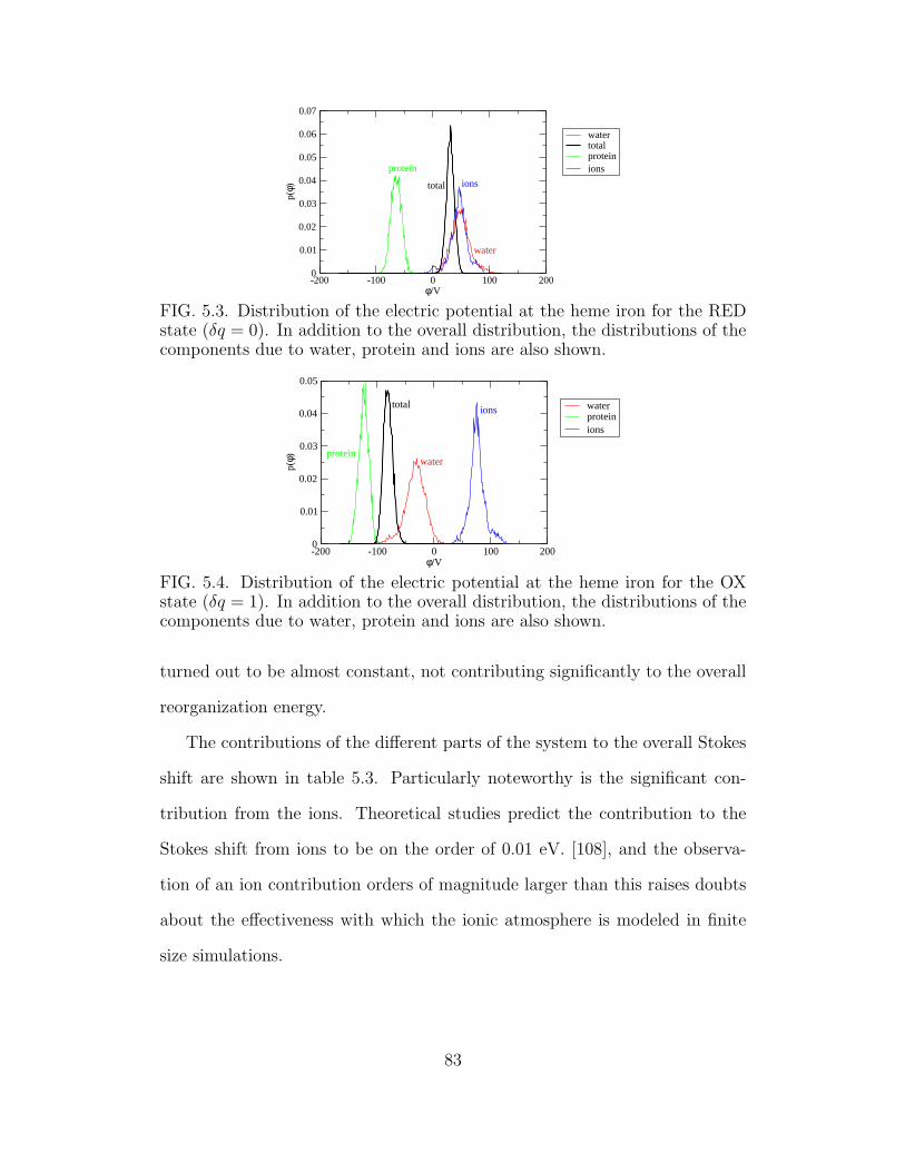
-200 -100 0 100 200φ/V

0

0.01

0.02

0.03

0.04

0.05

0.06

0.07

p(φ)

watertotalproteinions

ions

water

protein

total

FIG. 5.3. Distribution of the electric potential at the heme iron for the REDstate (δq = 0). In addition to the overall distribution, the distributions of thecomponents due to water, protein and ions are also shown.

-200 -100 0 100 200φ/V

0

0.01

0.02

0.03

0.04

0.05

p(φ)

waterproteinions

ions

waterprotein

total

FIG. 5.4. Distribution of the electric potential at the heme iron for the OXstate (δq = 1). In addition to the overall distribution, the distributions of thecomponents due to water, protein and ions are also shown.

turned out to be almost constant, not contributing significantly to the overall

reorganization energy.

The contributions of the different parts of the system to the overall Stokes

shift are shown in table 5.3. Particularly noteworthy is the significant con-

tribution from the ions. Theoretical studies predict the contribution to the

Stokes shift from ions to be on the order of 0.01 eV. [108], and the observa-

tion of an ion contribution orders of magnitude larger than this raises doubts

about the effectiveness with which the ionic atmosphere is modeled in finite

size simulations.

83

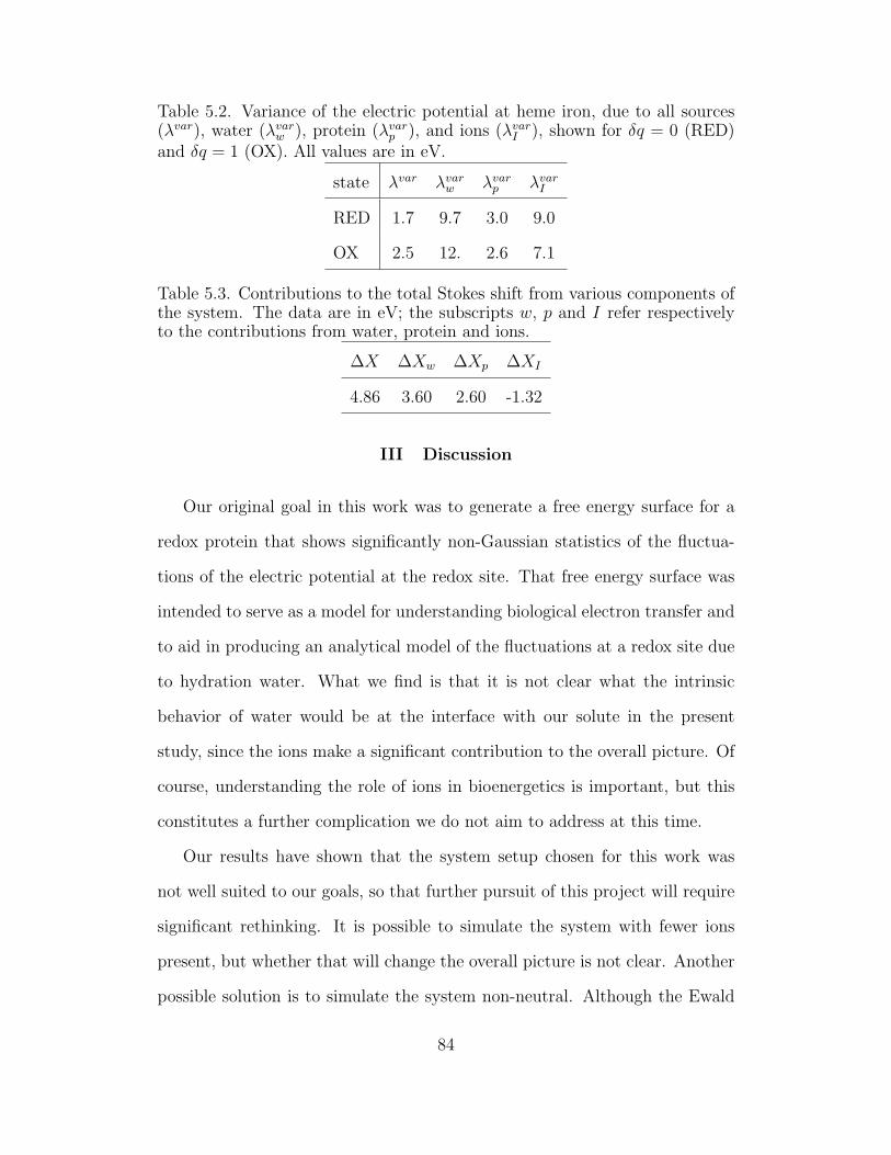
Table 5.2. Variance of the electric potential at heme iron, due to all sources(λvar), water (λvar

w ), protein (λvarp ), and ions (λvar

I ), shown for δq = 0 (RED)and δq = 1 (OX). All values are in eV.

state λvar λvarw λvar

p λvarI

RED 1.7 9.7 3.0 9.0

OX 2.5 12. 2.6 7.1

Table 5.3. Contributions to the total Stokes shift from various components ofthe system. The data are in eV; the subscripts w, p and I refer respectivelyto the contributions from water, protein and ions.

∆X ∆Xw ∆Xp ∆XI

4.86 3.60 2.60 -1.32

III Discussion

Our original goal in this work was to generate a free energy surface for a

redox protein that shows significantly non-Gaussian statistics of the fluctua-

tions of the electric potential at the redox site. That free energy surface was

intended to serve as a model for understanding biological electron transfer and

to aid in producing an analytical model of the fluctuations at a redox site due

to hydration water. What we find is that it is not clear what the intrinsic

behavior of water would be at the interface with our solute in the present

study, since the ions make a significant contribution to the overall picture. Of

course, understanding the role of ions in bioenergetics is important, but this

constitutes a further complication we do not aim to address at this time.

Our results have shown that the system setup chosen for this work was

not well suited to our goals, so that further pursuit of this project will require

significant rethinking. It is possible to simulate the system with fewer ions

present, but whether that will change the overall picture is not clear. Another

possible solution is to simulate the system non-neutral. Although the Ewald

84

sum is divergent in this case, it is possible to apply the correction to account

for the self-interaction of the system and its images[21].

The present results raise pragmatic concerns over setting up biomolecular

simulation. The large Stokes shift from ions observed here may be the result

of the extra charge added to the system to maintain neutrality. Or it may

simply be an artifact of the force field used. The behavior of ions in simulation

is notably strongly dependent on force field parameters[109, 110]. Therefore,

the observation of a significant contribution of ions to the quantities of interest

indicates the fundamental difficulty of obtaining “realistic” results for such a

system by molecular dynamics. We therefore emphasize that our goal in such

a project is to generate results for models with interesting behavior, in order

to map out the range of possible behaviors. It remains for experimentalists to

determine where specific systems fall in the range of possibilities.

Nevertheless, there are some points we learn from this set of simulations.

We have here at least one example of a case in which linear response is followed

relatively closely. We find that linear response is successful in the region near

δq = 0. We also note that the degree of nonlinearity observed in a charge

transfer process depends not only on whether the free energy surfaces are

nonlinear, but also on where the two states of interest lie on that curve.

85

Chapter 6

CONCLUSION

In our studies of water at the interface with nanometer-size solutes, we have

examined several properties, with an emphasis on the electrostatic properties

of the hydration layer. We have found that the polarity of water at the interface

is enhanced when compared to bulk water[23]. We quantify this polarity in

terms of the dielectric response of the hydration layer. The increased polarity

can be traced back to the increased density of water at the interface. Even

in the case of a hydrophobic solute that undergoes weak dewetting at the

interface, the collective dielectric response of the hydration layer is enhanced,

compared with bulk water. The implication is that one cannot effectively

model aqueous solutions as a simple superposition of components with different

dielectric constants, separated by a mathematical interface, as suggested by

continuum electrostatics. Depending on the question one asks, the effect may

or may not be critical. We find that the chemical potential of a dipole at the

center of a spherical solute in water approaches the prediction of continuum

electrostatics as the solute size increases. This is in contrast to what was found

previously for dipolar hard spheres, and it may therefore be due to the strength

of hydrogen bonds. On the other hand, the energy stored in the electric field

in the hydration layer of a nanometer size solute is expected to be enhanced

compared to the prediction of continuum electrostatics.

In contrast to solvation of a multipole at the center of the cavity, we have

found that when the statistics of the electric field fluctuations are probed near

the solute-water interface, the statistics become strongly non-Gaussian [111].

86

The result is an excess in fluctuations of the electric field at the interface.

This is the result of interfacial waters switching between different preferred

orientations. The excess fluctuations are associated with slow hydration dy-

namics. The region of excess fluctuations is quite broad, so that one expects

the phenomenon to be present in the hydration shells of a variety of solutes

with surface polar groups.

We have found, further, that when the interface is decorated with a collec-

tion of dipoles, the region characterized by excess fluctuations becomes broader

still. This phenomenon is due to the onset of a second, cooperative transition

in the interfacial waters. The excess fluctuations associated with the two tran-

sitions in the interfacial water lead to a broad range of dipole magnitudes

over which the scaling of the hydration free energy is approximately cubic,

rather than quadratic as continuum (or any linear response) models would

predict. This implies that continuum treatments of nanometer sized solutes

with polar domains at the interface will have the picture qualitatively wrong.

Consequently, even when continuum models are calibrated, they cannot be

expected to be robust. The solvation dynamics become quite slow, when the

hydration layer cooperatively switches between configurational states, spiking

to the nanosecond timescale in the vicinity of the transition.

The results have implications for biology. The nature of the hydration of

redox proteins is critical for understanding the energetics of biological elec-

tron transfer. The traditional picture of charge transfer reactions assumes the

solvent behaves like a dielectric in the linear regime. The observation of fluctu-

ations significantly in excess of the predictions of linear response for systems

with a significant polarity at the surface implies that this treatment is not

based on the right picture. Protein surfaces are characterized by regions of

87

high and low charge density; one therefore expects the overall solvation picture

to involve a combination of hydrophobic solvation (approximately harmonic)

and of the picture painted here of stronger scaling of the solvent response with

the solute polarity. The breaking of linear response implies that charge trans-

fer in biology may be more energetically efficient than the traditional picture of

redox would predict. Simulations of hydrated proteins have already indicated

a significantly non-Gaussian character of the fluctuations of the energy gap

for biological electron transfer reactions[5]. We demonstrate here that such

effects could be achieved, at least in part, due to water switching between

preferred states at the interface. Most likely, this is only one part of the pic-

ture for biological systems. The slow protein dynamics are known to couple

to the hydration water[97, 51], and seem to account for at least a significant

portion of the slow hydration dynamics. But a recent study of GFP has shown

that when the protein is frozen, a degree of non-Gaussianity is retained in the

solvent response at the chromophore[68].

88

REFERENCES

[1] P. Ball, Chem. Rev. 108, 74 (2008).

[2] P. L. Privalov, Crit. Rev. Biochem. Mol. Biol. 25, 5910 (1990).

[3] P. W. Fenimore, H. Frauenfelder, B. H. McMahon, and F. G. Parak,Proc. Natl. Acad. Sci. 99, 16047 (2002).

[4] N. Muneda, M. Shibata, M. Demura, and H. Kandori, J. Am. Chem.Soc. 128, 6294 (2006).

[5] D. N. LeBard and D. V. Matyushov, Phys. Chem. Chem. Phys. 12,15335 (2010).

[6] C. A. Angell, Nat. Mater. 11, 362 (2012).

[7] A. J. Patel et al., J. Phys. Chem. B 116, 2498 (2012).

[8] S. Sarupria and S. Garde, Phys. Rev. Lett. 103, 037803 (2009).

[9] D. Ben-Amotz and R. Underwood, Acc. Chem. Res. 41, 957 (2008).

[10] T. L. Beck, J. Stat. Phys. 145, 335 (2011).

[11] P. M. Chaikin and T. C. Lubensky, Principles of condensed matterphysics (Cambridge University Press, Cambridge, 1995).

[12] D. R. Martin and D. V. Matyushov, Phys. Rev. E 78, 041206 (2008).

[13] J. P. Hansen and I. R. McDonald, Theory of Simple Liquids (AcademicPress, Amsterdam, 2003).

[14] H.-A. Yu and M. Karplus, J. Chem. Phys. 89, 2366 (1988).

[15] H. Frohlich, Theory of dielectrics (Oxford University Press, Oxford,1958).

[16] M. Born, Z. Phys. 1, 45 (1920).

[17] L. Onsager, J. Am. Chem. Soc. 58, 1486 (1936).

[18] C. J. F. Bottcher, Theory of Electric Polarization Vol. 1 (Elsevier, Am-sterdam, 1973).

[19] S. Rajamani, T. Ghosh, and S. Garde, J. Chem. Phys. 120, 4457 (2004).

[20] H. S. Ashbaugh, J. Phys. Chem. B 104, 7235 (2000).

[21] G. Hummer, L. R. Pratt, and A. E. Garcia, J. Phys. Chem. 100, 1206(1996).

89

[22] W. M. Latimer, K. S. Pitzer, and C. M. Slansky, J. Chem. Phys. 258,349 (2000).

[23] A. D. Friesen and D. V. Matyushov, Chem. Phys. Lett. 511, 256 (2011).

[24] J. M. J. Swanson, S. A. Adcock, and J. A. McCammon, J. Chem. TheoryComput. 1, 484 (2005).

[25] M. Uematsu and E. U. Franck, J. Phys. Chem. Ref. Data 9, 1291 (1980).

[26] E. Condon, Phys. Rev. 28, 1128 (1926).

[27] A. Nitzan, Chemical Dynamics in Condensed Phases (Oxford UniversityPress, New York, 2006).

[28] D. V. Matyushov and M. D. Newton, J. Phys. Chem. A 105, 8516(2001).

[29] N. Mataga, Y. Kaifu, and M. Koizumi, J. Am. Chem. Soc. 29, 465(1956).

[30] E. L. Mertz, V. A. Tikhomirov, and L. I. Krishtalik, J. Phys. Chem. A101, 3433 (1997).

[31] L. D. Landau and E. M. Lifshitz, Electrodynamics of continuous media(Pergamon, Oxford, 1984).

[32] M. Neumann, J. Chem. Phys. 82, 5663 (1985).

[33] M. Neumann, Mol. Phys. 57, 97 (1986).

[34] M. Neumann, Chem. Phys. Lett. 95, 417 (1983).

[35] C. Y. Lee, J. A. McCammon, and P. J. Rossky, J. Chem. Phys. 80, 4448(1984).

[36] N. Giovambattista, P. G. Debenedetti, and P. J. Rossky, Chem. Phys.258, 349 (2000).

[37] G. M. Torrie and G. N. Patey, J. Phys. Chem. 97, 12909 (1993).

[38] K. A. Sharp and J. M. Vanderkooi, Acc. Chem. Res. 43, 231 (2010).

[39] P. J. Rossky and J. D. Simon, Science 370, 263 (1994).

[40] Y. R. Shen and V. Ostroverkhov, Chem. Rev. 106, 1140 (2006).

[41] G. Hummer, S. Garde, A. E. Garcia, and L. R. Pratt, Chem. Phys. 258,349 (2000).

[42] S. Garde, G. Hummer, A. E. Garcıa, M. E. Paulaitis, and L. R. Pratt,Phys. Rev. Lett. 77, 4966 (1996).

90

[43] K. Lum, D. Chandler, and J. Weeks, J. Phys. Chem. B 103, 4570 (1999).

[44] T. R. Jensen et al., Phys. Rev. Lett. 90, 086101 (2003).

[45] G. Hummer and S. Garde, Phys. Rev. Lett. 80, 4193 (1998).

[46] D. M. Huang and D. Chandler, J. Phys. Chem. B 106, 2047 (2002).

[47] R. Jimenez, G. R. Fleming, P. V. Kumar, and M. Maroncelli, Nature369, 471 (1994).

[48] S. K. Pal and A. H. Zewail, Chem. Rev. 104, 2099 (2004).

[49] O. Kwon, T. H. Yoo, C. M. Othon, J. A. Deventer, and A. H. Zewail,Trans. Faraday Soc. 57, 557 (1961).

[50] J. Tripathy and W. F. Beck, J. Phys. Chem. B 114, 15958 (2010).

[51] B. Halle and L. Nilsson, J. Phys. Chem. B 113, 8210 (2009).

[52] R. A. Marcus, J. Chem. Phys. 24, 966 (1956).

[53] R. A. Marcus, J. Chem. Phys. 26, 867 (1957).

[54] N. S. Hush, Trans. Faraday Soc. 57, 557 (1961).

[55] D. V. Matyushov, Chem. Phys. 351, 46 (2008).

[56] R. A. Marcus, J. Chem. Phys. 24, 979 (1956).

[57] A. Warshel, J. Phys. Chem. 86, 2218 (1982).

[58] J. C. Rasaiah and J. Zhu, J. Chem. Phys. 129, 214503 (2008).

[59] M. Cascella, A. Magistrato, I. Tavernelli, P. Carloni, and U. Rothlis-berger, Proc. Natl. Acad. Sci. 103, 19641 (2006).

[60] E. Solomon, R. Szilagyi, S. DeBeerGeorge, and L. Basumallick, Chem.Rev. 104, 419 (2004).

[61] A. Warshel and W. W. Parson, Quat. Rev. Biophys. 34, 563 (2001).

[62] D. N. LeBard and D. V. Matyushov, J. Phys. Chem. B 112, 5218 (2008).

[63] D. N. LeBard and D. V. Matyushov, J. Phys. Chem. B 113, 12424(2009).

[64] H. B. Gray and J. R. Winkler, Proc. Natl. Acad. Sci. 102, 3534 (2005).

[65] I. Muegge, P. X. Qi, A. J. Wand, Z. T. Chu, and A. Warshel, J. Phys.Chem. B 101, 825 (1997).

[66] W. W. Parson, Z. T. Chu, and A. Warshel, Biophys. J. 74, 182 (1998).

91

[67] P. K. Ghorai and D. V. Matyushov, J. Am. Chem. Soc. 127, 16390(2005).

[68] D. R. Martin and D. V. Matyushov, Non-gaussian statistics and nanosec-ond dynamics of electrostatic fluctuations affecting optical transitions inproteins, submitted,J. Phys. Chem. B .

[69] G. Hummer, L. R. Pratt, and A. E. Garcia, J. Phys. Chem. A 102, 7885(1998).

[70] D. Chandler and J. P. Garrahan, J. Chem. Phys. 123, 044511 (2005).

[71] D. Chandler, Nature 437, 640 (2005).

[72] N. Giovambattista, C. F. Lopez, P. J. Rossky, and P. G. Debenedetti,Proc. Natl. Acad. Sci. 105, 2274 (2008).

[73] M. S. A. Kader, Chem. Phys. 281, 49 (2002).

[74] T. Kihara, Rev. Mod. Phys. 25, 831 (1953).

[75] H. J. C. Berendsen, J. R. Grigera, and T. P. Straatsma, J. Phys. Chem.91, 6269 (1987).

[76] W. Smith and T. R. Forester, J. Molec. Graphics 14, 136 (1996).

[77] R. Schmid and D. V. Matyushov, J. Phys. Chem. 99, 2393 (1995).

[78] J. Mittal and G. Hummer, Proc. Natl. Acad. Sci. 105, 20130 (2008).

[79] V. P. Sokhan and D. J. Tildesley, Mol. Phys. 92, 625 (1997).

[80] A. Papazyan and A. Warshel, J. Chem. Phys. 107, 7975 (1997).

[81] V. Ballenegger and J.-P. Hansen, J. Phys. Chem. 122, 114711 (2005).

[82] H. K. W. Y. Martin, D. W. Abraham, Appl. Phys. Lett. 52, 1103 (2007).

[83] T. Fukuma, Sci. Tech. Adv. Mater. 11, 033003 (2010).

[84] T. Uchihashi, M. Higgins, Y. Nakayama, J. E. Sader, and S. P. Jarvis,Sci. Tech. Adv. Mater. 16, S49 (2005).

[85] T. Hiasa et al., J. Phys. Chem. C 14, 21423 (2010).

[86] M. Tachiya, Chem. Phys. Lett. 203, 164 (1993).

[87] L. D. Landau and E. M. Lifshits, Statistical Physics (Pergamon Press,New York, 1980).

[88] K. A. Sharp and B. Madan, J. Phys. Chem. B 101, 4343 (1997).

92

[89] C. Vega, E. Sanz, and J. L. F. Abascal, J. Chem. Phys. 122, 114507(2005).

[90] M. S. S. Challa, D. P. Landau, and K. Binder, Phys. Rev. B 34, 1841(1986).

[91] A. Laaksonen, P. G. Kusalik, and I. M. Svishchev, J. Phys. Chem. A101, 5910 (1997).

[92] R. Blinc and B. Zeks, Soft modes in ferroelectrics and antiferroelectrics(North-Holland Publishing Co., Amsterdam, 1974).

[93] K. Binder and D. W. Heermann, Monte Carlo simulation in statisticalmechanics (Springer-Verlag, Berlin, 1992).

[94] D. van der Spoel, P. J. van Maaren, P. Larsson, and N. Timneanu, J.Phys. Chem. B 101, 4343 (1997).

[95] P. Abbyad et al., J. Phys. Chem. B 111, 8269 (2007).

[96] D. V. Matyushov, J. Phys. Chem. B 115, 10715 (2011).

[97] S. Sen, D. Andreatta, S. Y. Ponomarev, D. L. Beveridge, and M. A.Berg, J. Am. Chem. Soc. 131, 1724 (2009).

[98] J. C. Philips et al., J. Comput. Chem. 26, 1781 (2005).

[99] W. D. Cornell et al., J. Am. Chem. Soc. 117, 5179 (1995).

[100] G. Chopra and M. Levitt, Proc. Natl. Acad. Sci. (2011).

[101] P. Gallo, M. Rovere, and E. Spohr, Phys. Rev. Lett. 85, 4317 (2000).

[102] K. Binder, Rep. Prog. Phys. 50, 783 (1987).

[103] H. E. Stanley, Introduction to phase transitions and critical phenomena(Oxford University Press, New York, 1987).

[104] D. V. Matyushov and B. M. Ladanyi, J. Chem. Phys. 110, 994 (1999).

[105] J. A. D. MacKerrell et al., J. Phys. Chem. B 102, 3586 (1998).

[106] S. Kumar, K. Bouzida, R. Swendsen, P. Kollman, and J. Rosenberg, J.Comp. Chem. 13, 1012 (1992).

[107] D. W. Small, D. V. Matyushov, and G. A. Voth, J. Am. Chem. Soc.125, 7470 (2003).

[108] J. J. Zhu, R. Ma, Y. Lu, and G. Stell, J. Chem. Phys. 123, 224505(2005).

[109] P. Auffinger, T. E. Cheatham III, and A. C. Vaiana, J. Chem. TheoryComput. 3, 1851 (2007).

93

[110] I. S. Joung and T. E. Cheatham III, J. Phys. Chem. B 112, 9020 (2008).

[111] A. D. Friesen and D. V. Matyushov, J. Chem. Phys. 135, 104501 (2011).

[112] H. J. C. Berendsen, J. P. M. Postma, W. van Bunsteren, A. DiNola, andJ. R. Haak, J. Chem. Phys. 81, 3684 (1984).

[113] T. Morishita, J. Chem. Phys. 113, 2976 (2000).

[114] P. H. Hunenberger, Thermostat algorithms for molecular dynamics sim-ulations, in Advanced Computer Simulation, edited by C. Dr. Holmand K. Prof. Dr. Kremer, , Advances in Polymer Science Vol. 173, pp.105–149, Springer Berlin / Heidelberg, 2005.

[115] A. Glattli, X. Duara, and W. F. van Gunsteren, J. Chem. Phys. 116,9811 (2002).

94

Appendix A

SIMULATION PROTOCOL FOR NON-POLAR KIHARA CAVITIES

95

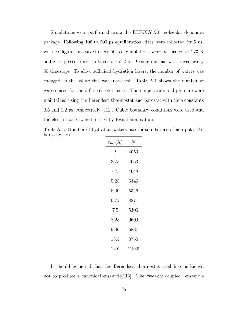
Simulations were performed using the DLPOLY 2.0 molecular dynamics

package. Following 100 to 500 ps equilibration, data were collected for 5 ns,

with configurations saved every 50 ps. Simulations were performed at 273 K

and zero pressure with a timestep of 2 fs. Configurations were saved every

50 timesteps. To allow sufficient hydration layers, the number of waters was

changed as the solute size was increased. Table A.1 shows the number of

waters used for the different solute sizes. The temperature and pressure were

maintained using the Berendsen thermostat and barostat with time constants

0.5 and 0.2 ps, respectively [112]. Cubic boundary conditions were used and

the electrostatics were handled by Ewald summation.

Table A.1. Number of hydration waters used in simulations of non-polar Ki-hara cavities.

r0s (A) N

3 4053

3.75 4053

4.5 4048

5.25 5346

6.00 5346

6.75 8871

7.5 5306

8.25 9699

9.00 5887

10.5 8750

12.0 11845

It should be noted that the Berendsen thermostat used here is known

not to produce a canonical ensemble[113]. The “weakly coupled” ensemble

96

actually is somewhere in between the microcanonical and canonical ensembles

[113, 114]. We have checked for a few representative points that no significant

changes to the results were produced in simulations at constant energy. The

dependence of the results on system size was also checked. Our system sizes are

in the range where the finite size effect on the reported quantities is negligible.

Nevertheless, one must be aware that in general fluctuations can depend on

the ensemble used, and we have not strictly checked against a true canonical

ensemble. However, it is encouraging to note that our results for the bulk

dielectric constant are close to those reported in existing literature[115], and

that the results for the chemical potential tend to the expected limit for large

cavities.

97

Appendix B

SIMULATION PROTOCOL FOR KIHARA CAVITY WITH DIPOLE

98

Nanoscale solutes in water were modeled by the insertion spherical particles

in SPC/E water. The solutes consist of a hard-sphere (HS) core, surrounded

by a Lennard-Jones (LJ) layer. The interactions of this solute with SPC/E

water oxygen are given by a potential of the Kihara type:

φ0s(r) = 4ǫ0s

[

(

σ0s

r − rHS

)12

−

(

σ0s

r − rHS

)6]

. (B.1)

In the present study, the values of of the parameters were: rHS = 9 A, σ0s =

3 A, and ǫ0s = 0.65 kJ/mol. A point dipole was placed at the distance, rd

from the solute center. The dipole was oriented along the radial direction,

with the positive end of the dipole toward the interface. The distance from

the dipole to the interface is indicated by rds. We studied solutes with rd = 9

A and rd = 10 A. The dipole magnitude, m0 was varied between 0 and 10

Debye. Simulations were performed at 273 K and 1 atm with 11845 hydration

waters. The temperature and pressure were maintained using the Berendsen

thermostat and barostat [112]. Most trajectories were 1 ns long following

equilibration, although representative points were simulated to 5 ns to check for

convergence. Note that the use of the Berendsen thermostat does not produce

kinetic energy fluctuations consistent with the canonical ensemble[113]. We

expect that the effect on the present results is minimal (see Appendix A for

details), but we have not proven this rigorously.

99

Appendix C

THREE-STATE PHENOMENOLOGICAL MODEL

100

We introduce a model in which the free energy of fluctuations of the reac-

tion field, R, are given by the superposition of three states, g, 1, 2:

e−βF(m0,R) = e−βFg(m0,R) + e−βF1(m0,R) + e−βF2(m0,R), (C.1)

where:

Fg(m0, R) =R2/(2κg)−m0R

F1(m0, R) =−m0R + (R−R1)2/(2κ1) + F1

F2(m0, R) =−m0R + (R−R2)2/(2κ2) + F2, (C.2)

where κg,1,2 are the response functions of the solvent. F1,2 is the free energy

cost for reaching the excited state and R1,2 is the spontaneous reaction field

in the excited state.

The average field and variance are found by the usual means:

〈Rn〉 = Q−1

∫

dR Rn e−βF(R) (C.3)

where Q =∫

dR e−βF(R). We get for the average:

〈R〉 = ngκgm0 + n1(κ1m0 +R1) + n2(κ2m0 +R2), (C.4)

and for the variance:

〈(δR)2〉 =kT (ngκg + n1κ1 + n2κ2)

+ n1ng (m0(κ1 − κg) +R1)2 + n2ng (m0(κ2 − κg) +R2)

2

+ n1n2 (m0(κ2 − κ1) +R2 −R1)2 . (C.5)

101

In [Eq. (C.4)] and [Eq. (C.5)], ng, n1 and n2 are the fractional populations of

the three states:

n−1g =1 +

√

κ1

κg

eβ[m2

0(κ1−κg)/2+m0R1−F1] +

√

κ2

κg

eβ[m2

0(κ2−κg)/2+m0R2−F2]

n−11 =1 +

√

κ2

κ1

eβ[m2

0(κ2−κ1)/2+m0(R2−R1)+F1−F2] +

√

κg

κ1

eβ[m2

0(κg−κ1)/2−m0R1)+F1]

n−12 =1 +

√

κ1

κ2

eβ[m2

0(κ1−κ2)/2+m0(R1−R2)+F2−F1] +

√

κg

κ2

eβ[m2

0(κg−κ2)/2−m0R2)+F2].

(C.6)

102

Appendix D

BOUNDARY VALUE PROBLEM FOR AN OFF-CENTER DIPOLE

INSIDE A SPHERICAL CAVITY IN A DIELECTRIC

103

To find the dielectric response to a dipole off-center, we begin by calculating

the potential due to a point charge, q at an arbitrary point inside a sphere

with dielectric constant, ǫ1, immersed in a material with dielectric constant,

ǫ2. The radius of the sphere is r0s, and the location of the charge is s. The

potential at the point, r must satisfy the Poisson equation:

ǫ1∆φ1 =− 4πρ

ǫ2∆φ2 =− 4πρ, (D.1)

where φ1 is the potential inside the sphere, and φ2 is the potential outside the

sphere. The solution has the following form:

φ = φ0 + φR =1

ǫ1

1

|r− s|+ φR, (D.2)

where φ0 is the simple Coulomb interaction with the point charge and φR

is the reaction potential from the surrounding dielectric. Expanding in the

Legendre polynomials,

φR1 =

∞∑

l=0

AlrlPl(cos θ)

φR2 =

∞∑

l=0

Bl

rl+1Pl(cos θ)

φ0 =

∑

∞

l=01ǫ1r

(

rs

)l+1Pl(cos θ), s > r

∑

∞

l=01ǫ1r

(

sr

)l+1Pl(cos θ), r > s

(D.3)

The boundary conditions are:

φ1(r0s) = φ2(r0s), (D.4)

and:

ǫ1∂φ1

∂r

∣

∣

∣

∣

r=r0s

= ǫ2∂φ2

∂r

∣

∣

∣

∣

r=r0s

. (D.5)

104

Respectively, these require :

Al(r0s)l = Bl/(r0s)

l+1, (D.6)

and:

ǫ1lAl(r0s)l−1 −

(l + 1)sl

(r0s)l+2= −

ǫ2ǫ1

(l + 1)sl

(r0s)l+2−

ǫ2(l + 1)Bl

(r0s)l+2. (D.7)

The reaction potential inside the sphere is (dropping the subscript):

φ = −qǫ− 1

r0s

∞∑

l=0

Gl

(

rs

(r0s)2

)l

Pl(cos θ), (D.8)

where ǫ = ǫ2/ǫ1, and:

Gl =l + 1

l (ǫ+ 1) + ǫ. (D.9)

The reaction field from a collection of charges qi at points si is found from

the gradient of the reaction potential:

R0 = −∇rφR

=ǫ− 1

r r0s

∑

i

qi

∞∑

l=0

Gl

(

r si(r0s)2

)l[

lPl(cos θ)r− P′

l (cos θ) (s− r(s · r))]

.

(D.10)

The first term in the square brackets is the longitudinal (radial) projection,

and the second term is the transverse projection. For a dipole along the radial

unit vector (cos θ = 1), we have two charges, q1 and q2, at distances s1 and

s2 = s1 +∆s from the cavity center. The reaction field is:

R0 =ǫ− 1

r r0s

∑

i

qi

∞∑

l=1

l Gl

(

r si(r0s)2

)l

=ǫ− 1

(r0s)3

∞∑

l=1

Gl

(

r

(r0s)2

)l−1

q(

sl − (s+∆s)l)

, (D.11)

105

where q = |q1| = |q2| and s = s1. In the limit of small ∆s:

q(

sl − (s+∆s)l)

≈ q (∆s) sl−1 l = −l m0 sl−1, (D.12)

where m0 = q∆s is the dipole moment. The reaction field due to the point

dipole is:

R0 = m0ǫ− 1

r0s

∞∑

l=1

l2 Gl

(

rs

(r0s)2

)l−1

. (D.13)

For small r, s, the sum converges quickly, and we have:

Gl ≈ G1 = 2/(2ǫ+ 1). (D.14)

Thus, letting r → s, in the limit of small s, the reaction field at the dipole is:

R0 = m02(ǫ− 1)

(2ǫ+ 1)(r0s)3

∞∑

l=1

l2(

s2

(r0s)2

)l−1

. (D.15)

Representing (s/r0s)2 = t, the summation can be written in terms of the

geometric series:

d

dt

(

td

dt

∞∑

l=0

tl

)

=d

dt

(

td

dt

1

1− t

)

, (D.16)

and we obtain:

R0 = R(0) = m02(ǫ− 1)

(2ǫ+ 1)(r0s)3×

1 + z2

(1− z2)3, (D.17)

where z = s/r0s. For s/r0s close to 1, the series converges slowly, and the

factors Gl are given by their limiting value for large l:

Gl ≈ 1/(ǫ+ 1). (D.18)

In this case, we get:

R0 = R(1) = m0ǫ− 1

(ǫ+ 1)(r0s)3×

1 + z2

(1− z2)3. (D.19)

106

For the more general case, 0 < s < r0s, we can write:

R0 = R(0) + h(z)(

R(1) −R(0))

(D.20)

where h(z) =[

R0 −R(0))

/(

R(1) −R(0)]

. h(z) can be expanded in the even

powers of z. To a good approximation, h(z) ≈ z2; then the reaction field for

0 < s < r0s is:

R0 = m0ǫ− 1

(2ǫ+ 1)(r0s)3×

(

2−z2

ǫ+ 1

)

×1 + z2

(1− z2)3. (D.21)

For the comparison of the simulation results with continuum electrostatics,

we have used the value, r0s = 11.5 A, on the basis of the following criteria:

1. The first peak of the solute-oxygen radial distribution function occurs

around r ≈ rHS+σ0s = 12 A, although fluctuations bring water molecules

to marginally closer distances, since the interface is soft.

2. As the solvent structure is perturbed by the field from the solute dipole,

a new feature in the solute-solvent pair correlation function appears at

approximately 11 A from the cavity center. Taking the midpoint between

11 A and 12 A is therefore a reasonable estimate of the continuum radius.

3. The local solvent response was expected to scale approximately with the

field from the solute dipole at the interface. We found the proper scaling,

(rds)−3 was produced when r0s is taken to be 11.5 A.

We therefore concluded that r0s ≈ 11.5 A is a physically sensible value for

r0s, although we stress that the difficulty in rigorously determining a value for

the continuum radius only reinforces the inadequacy of continuum electrostat-

ics at the molecular level.

107

Appendix E

SOLID ANGLE

108

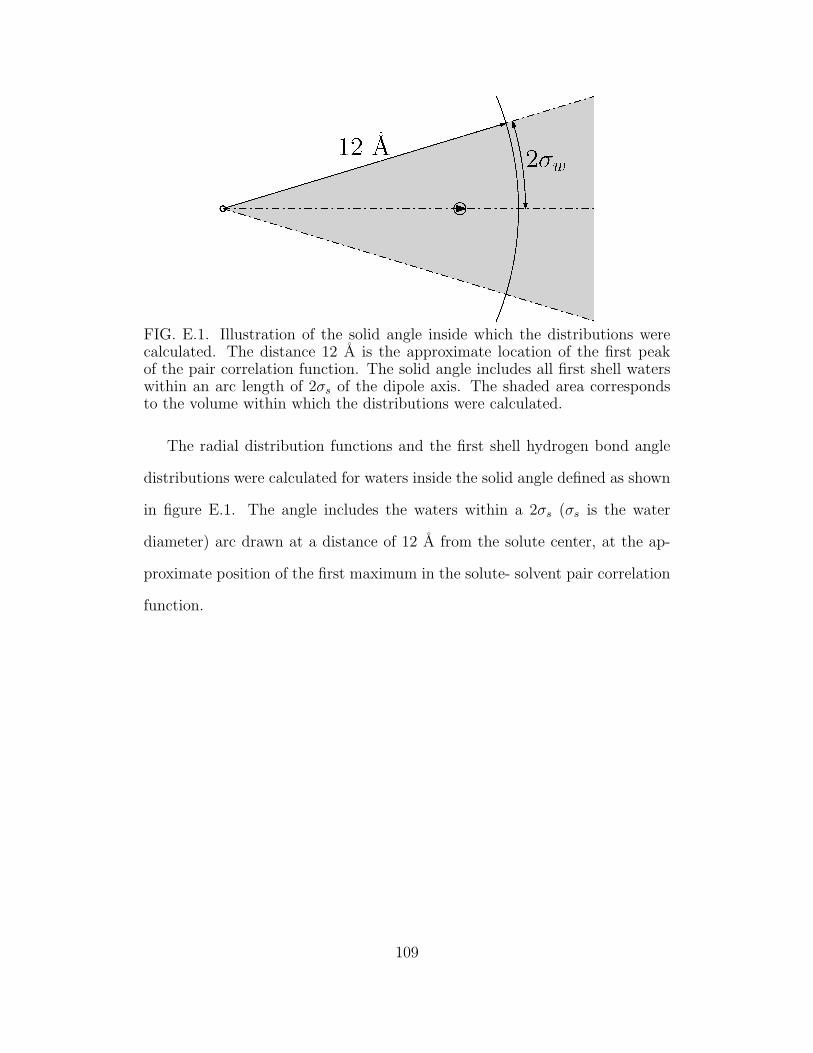
FIG. E.1. Illustration of the solid angle inside which the distributions werecalculated. The distance 12 A is the approximate location of the first peakof the pair correlation function. The solid angle includes all first shell waterswithin an arc length of 2σs of the dipole axis. The shaded area correspondsto the volume within which the distributions were calculated.

The radial distribution functions and the first shell hydrogen bond angle

distributions were calculated for waters inside the solid angle defined as shown

in figure E.1. The angle includes the waters within a 2σs (σs is the water

diameter) arc drawn at a distance of 12 A from the solute center, at the ap-

proximate position of the first maximum in the solute- solvent pair correlation

function.

109

Appendix F

DIPOLAR RESPONSE OF A SUBVOLUME

110

Here we derive the expression for the dipolar susceptibility of a subvolume

to a uniform applied electric field. For simplicity, we take the field E0 to be

along the z direction: E0 = E0 · z = |E0|. We then focus on the statistics of

M = M · z. The dipole moment of the sample in the absence of an applied

field will fluctuate with the probability distribution:

p0(M) ∝

∫

dΓ e−βH0(Γ)δ(M(Γ)−M). (F.1)

Where H0(Γ) is the total system Hamiltonian in the absence of an applied

field, at the point Γ in phase space. When a field is applied, the energy is

modified to:

H(Γ, E0) = −ME0 +H0(Γ). (F.2)

Because we are interested in a subvolume, we set M = MΩ+M2, where MΩ is

the dipole moment in the subvolume under consideration and M2 is the dipole

of the rest of the sample. We can then calculate the thermodynamic average

of MΩ:

〈MΩ〉 = Q−1

∫

dΓ eβME0−βH0(Γ)MΩ, (F.3)

where

Q =

∫

dΓ eβME0−βH0(Γ) (F.4)

111

is the canonical partition function. The susceptibility can then be found by

differentiation:

χΩ = Ω−1∂〈M〉

∂E0

= Ω−1Q−1

∫

dΓ βe−βH(Γ,E0)MΩM−

−Q−2

(∫

dΓ βe−βH(Γ,E0)M

)

×

(∫

dΓ e−βH(Γ,E0)MΩ

)

=β

Ω(〈MΩM〉 − 〈MΩ〉〈M〉)

=β

Ω〈δMΩδM〉. (F.5)

The fluctuations of the field are symmetric under rotation, so that 〈δMΩδM〉 =

〈δMΩ · δM〉/3, and we get

χΩ =β

3Ω〈δMΩ · δM〉. (F.6)

112

Appendix G

SIMULATION PROTOCOL FOR FULLERENE

113

The solute with the geometry of C180 was simulated using the NAMD

2 package[98] with 37924 hydration waters. The fullerene was modeled as a

rigid solute, with atoms of the type CA from the AMBER force field.[99] Water

was represented with the SPC/E model.[75] The temperature was maintained

at 310 Kelvin using a Langevin thermostat. Simulations were performed with

cubic periodic boundary conditions, and electrostatics were handled by particle

mesh Ewald. The system was hydrated in 37924 waters and each system was

equilibrated for 5 to 10 ns, before 40 ns production runs. The dipoles on the

carbon atoms were represented by two point charges separated by the distance

0.2 A. At the closest water approach, this makes a difference in the field of

less than ∼ 0.3%, compared with a true point dipole, and allows the use of

the standard integration routines in NAMD.

114

Appendix H

SIMULATION PROTOCOL FOR CYTOCHROME B562

115

The protein data bank (PDB) structure 256B was used to build Cytochrome

B562 for simulation. The CHARMM all atom force field was used, and the

system was hydrated in 33268 TIP3P water molecules. Ions were added to neu-

tralize the system at an ion concentration of 0.1 M. For each umbrella sampling

point, the extra charge δq was added to the HEME iron. The balancing charge

−δq was added to a sodium ion, so that the charge on the sodium ion ranged

between -0.6 and 1.6. At each umbrella sampling point, the system was first

equilibrated in the NPT ensemble at 1 atm, for 1 ns, then in the NVT ensem-

ble for 7 ns, with a 2 fs timestep. Following equilibration, production runs

were 13 ns trajectories in the NVT ensemble at 310 K, with the temperature

maintained using a Langevin thermostat. Cubic periodic boundary conditions

were used, and the electrostatics were handled by particle mesh Ewald.

116