The Astrophysical Journal, 783:79 (16pp), 2014 March 10 doi:10.1088/0004-637X/783/2/79C© 2014. The American Astronomical Society. All rights reserved. Printed in the U.S.A.

ELEMENTAL COMPOSITIONS OF TWO EXTRASOLAR ROCKY PLANETESIMALS∗

S. Xu (���)1, M. Jura1, D. Koester2, B. Klein1, and B. Zuckerman11 Department of Physics and Astronomy, University of California, Los Angeles, CA 90095-1562, USA; sxu@astro.ucla.edu,

jura@astro.ucla.edu, kleinb@astro.ucla.edu, ben@astro.ucla.edu2 Institut fur Theoretische Physik und Astrophysik, University of Kiel, D-24098 Kiel, Germany; koester@astrophysik.uni-kiel.de

Received 2013 September 23; accepted 2014 January 15; published 2014 February 19

ABSTRACT

We report Keck/HIRES and Hubble Space Telescope/COS spectroscopic studies of extrasolar rocky planetesimalsaccreted onto two hydrogen atmosphere white dwarfs, G29-38 and GD 133. In G29-38, eight elements are detected,including C, O, Mg, Si, Ca, Ti, Cr, and Fe while in GD 133, O, Si, Ca, and marginally Mg are seen. These twoextrasolar planetesimals show a pattern of refractory enhancement and volatile depletion. For G29-38, the observedcomposition can be best interpreted as a blend of a chondritic object with some refractory-rich material, a resultfrom post-nebular processing. Water is very depleted in the parent body accreted onto G29-38, based on the derivedoxygen abundance. The inferred total mass accretion rate in GD 133 is the lowest of all known dusty white dwarfs,possibly due to non-steady state accretion. We continue to find that a variety of extrasolar planetesimals all resembleto zeroth order the elemental composition of bulk Earth.

Key words: planetary systems – stars: abundances – white dwarfs

Online-only material: color figures

1. INTRODUCTION

Based upon models of planet formation, we understandthe variety of elemental compositions of planetesimals as afamiliar three step process (McSween & Huss 2010). (1) Undernebular condensation, incorporation of an element into theplanetesimal is a function of local temperature and pressure.(2) Differentiation often occurs, redistributing all elementswithin the planetesimal; lithophile elements (Al, Ca, Ti) areenhanced in the crust while siderophile elements (Fe, Mn, Cr,Ni) settle into the core. (3) Collisions lead to stripping andblending of cores and crusts, redistributing elements withinthe entire planetary system. In the solar system, chondrites area direct consequence of nebular condensation, i.e., step (1);achondrites and primitive achondrites have experienced post-nebular processing, i.e., steps (2) and (3) (O’Neill & Palme2008). The study of externally polluted white dwarfs providesinvaluable information about the elemental compositions ofextrasolar rocky planetesimals, directly testing these models,and contrasting with solar system objects (Jura 2013; Jura &Young 2014).

The current picture is that beyond a few AUs, a largefraction of extrasolar planetesimals can survive to the whitedwarf phase (Jura 2008). From dynamical rearrangement duringthe post-asymptotic giant branch phase, some planetesimalscan be perturbed into the tidal radius of the white dwarf andsubsequently “pollute” its pure hydrogen or helium atmosphere(Debes & Sigurdsson 2002; Jura 2003; Bonsor et al. 2011;Debes et al. 2012b; Veras et al. 2013). Calcium, the most easilydetected element from optical surveys, has been identified inover 200 white dwarfs (Zuckerman et al. 2003, 2010; Koesteret al. 2005; Dufour et al. 2007; Koester et al. 2011). So far, 30heavily polluted white dwarfs have been found to show excessinfrared radiation coming from the debris of these pulverized

∗ Some of the data presented herein were obtained at the W.M. KeckObservatory, which is operated as a scientific partnership among the CaliforniaInstitute of Technology, the University of California and the NationalAeronautics and Space Administration. The Observatory was made possibleby the generous financial support of the W.M. Keck Foundation.

planetesimals (e.g., Mullally et al. 2007; Farihi et al. 2009; Xu& Jura 2012, and references therein). These stars always show10 μm circumstellar silicate emission features when observedspectroscopically (Reach et al. 2005, 2009; Jura et al. 2009).Orbiting gaseous material has been detected in nine pollutedwhite dwarfs (Gansicke et al. 2006, 2007, 2008, 2012; Gansicke2011; Melis et al. 2010, 2012; Farihi et al. 2012a; Debes et al.2012a). With high-resolution spectroscopic observations, 19heavy elements have been detected in white dwarf atmospheres,including C, O, Na, Mg, Al, Si, P, S, Ca, Sc, Ti, V, Cr, Mn, Fe,Co, Ni, Cu, and Sr (Zuckerman et al. 2007; Klein et al. 2010,2011; Dufour et al. 2010, 2012; Farihi et al. 2010; Melis et al.2010; Vennes et al. 2010, 2011; Zuckerman et al. 2011; Juraet al. 2012; Gansicke et al. 2012; Xu et al. 2013a).

Theoretical calculations show that extrasolar planetesimalswith internal water can survive the red giant stage of their parentstar (Jura & Xu 2010). We can constrain the water mass fractionin extrasolar planetesimals by determining the abundance ofaccreted hydrogen and/or oxygen in polluted white dwarfs(Klein et al. 2010). By analyzing the hydrogen abundance inan ensemble of helium-dominated white dwarfs, Jura & Xu(2012) found that water is less than 1% of the total accretedmaterial. Recently, Farihi et al. (2013) identified a white dwarfwhich has accreted a large amount of oxygen, in excess of whatcan be combined into MgO, SiO2, FeO, CaO, and Al2O3; theyconcluded that the accreted asteroid is at least 26% water bymass. In addition, if there is enough water in the disk, molecularwater emission lines might be detectable in the near-infrared,similar to those around T Tauri stars (Carr & Najita 2008).

In this paper, we focus on two pulsating ZZ Ceti hy-drogen white dwarfs, G29-38 (WD 2326+049) and GD 133(WD 1116+026). G29-38 is a fascinating white dwarf and arecord holder. It is the first and also the closest white dwarf iden-tified with an infrared excess (Zuckerman & Becklin 1987) and a10 μm circumstellar silicate emission feature (Reach et al. 2005,2009). It is among the very first few hydrogen white dwarfs thatwere found to be polluted (Koester et al. 1997), which led tothe identification of a white dwarf subclass “DAZ” (Zuckermanet al. 2003). Very recently, G29-38, together with GD 133 and

1

The Astrophysical Journal, 783:79 (16pp), 2014 March 10 Xu et al.

Table 1Observation Logs

Star UT Date Instrument λ Range Exposure(Å) (s)

G29-38 2006 Jun 11 HIRES/red 5690–10160 7,2002008 Aug 7 HIRES/blue 3115–5950 2,0002010 Oct 17 COS 1145–1445 1,9992011 Jan 19 COS 1145–1445 7,0352011 Aug 15 NIRSPEC 27,500–36,000 2,160

GD 133 2008 Feb 13 HIRES/blue 3135–5965 2,7002008 Feb 26 HIRES/red 4600–8995 2,4002011 May 28 COS 1145–1445 13,460

GD 31 are the first white dwarfs with photospheric detectionsof molecular hydrogen (Xu et al. 2013b). The atmospheric pol-lution in GD 133 was first reported in the SPY survey (Koesteret al. 2005; Koester & Wilken 2006). It also has an orbiting dustdisk as well as a 10 μm silicate feature (Jura et al. 2007, 2009).

The paper is organized as follows. In Section 2, we report dataacquisition and reduction methods. In Section 3, we determinestellar parameters for G29-38 and GD 133. The heavy elementabundances are reported in Section 4. In Section 5, we comparethe composition of the parent body accreted onto G29-38 andGD 133 with solar system objects. In Section 6, we put ourresults in perspective and conclusions are given in Section 7.

2. OBSERVATIONS

We performed spectroscopic studies of G29-38 and GD 133with the High Resolution Echelle Spectrometer (HIRES) on theKeck telescope and the Cosmic Origins Spectrograph (COS) onthe Hubble Space Telescope (HST). G29-38 was also observedwith the NIRSPEC on the Keck telescope. The observation logsare presented in Table 1 and described in detail below.

2.1. Keck/HIRES Optical Spectroscopy

The optical data were acquired with HIRES (Vogt et al. 1994)on the Keck I telescope at Mauna Kea Observatory under goodweather conditions except for the night of 2008 August 7, wherehigh cirrus clouds were present that caused 2–3 magnitudes ofextinction. The C5 slit with a width of 1.′′148 was used for allobservations. The spectral resolution is ∼40,000 as measuredfrom the Th–Ar lamps.

The MAKEE software3 was used to extract the spectrafrom the flat-fielded two-dimensional image of each exposurewith the trace of a bright calibration star. Wavelength calibrationwas performed using the standard Th–Ar lamps. FollowingKlein et al. (2010, 2011), we used IRAF to normalize thespectra and combine echelle orders. When multiple exposureswere present, each exposure was processed separately based onsteps outlined above and combined afterward, weighted by theircount rates. For GD 133, there was second order contaminationin 8200–9000 Å region and we followed Klein et al. (2010) tocalibrate and extract that part of the spectrum. For both stars, thefinal spectra were continuum-normalized but not flux calibrated.The signal-to-noise ratio (S/N) for G29-38 is 50–90 shortwardof 3850 Å and 90-210 for longer wavelengths. For GD 133, theS/N is 30–60 shortward of 3900 Å and longward of 6000 Å and60–110 for the rest.

3 MAKEE Keck Observatory HIRES Data Reduction Software,http://www2.keck.hawaii.edu/inst/common/makeewww/.

2.8 2.9 3 3.1 3.2 3.3 3.4 3.5 3.6 3.7

1

3

5

7

9

11

13

15

λ (μm)

Fν

(mJy

)

Figure 1. Keck/NIRSPEC KL band spectrum for G29-38 and flux calibratedto IRAC 3.6 μm photometry. The spectral resolution is 2000 and the data areneither binned nor smoothed. The noisy region shortward of 2.9 μm is due tobright sky background and the emission around 3.3 μm is from an instrumentalartifact. The spectrum is generally featureless with a gentle increase towardlonger wavelength, consistent with the dust disk model.

2.2. HST/COS Ultraviolet Spectroscopy

G29-38 and GD 133 were observed as part of the HST cycle18 program 12290, “Do Rocky Extrasolar Minor Planets Havea Composition Similar to Bulk Earth?.” G29-38 was observedat two different times due to the malfunction of a gyro duringpart of the first observation. Instrument configuration and datareduction procedures were described in Xu et al. (2013b).Following Jura et al. (2012), we extracted night-time portions ofthe data to remove geocoronal O i emission lines near 1304 Å.For GD 133, there were 4711 s of useful night time data and theS/N of the unsmoothed spectrum is eight around O i 1304 Å.For G29-38, there are only 400 s of effective night time exposureand the data were not used for the analysis.

2.3. Keck/NIRSPEC Infrared Spectroscopy

G29-38 was observed with the NIRSPEC (McLean et al.1998, 2000) on the Keck II telescope in low resolution R ∼2000 spectroscopy mode and a central wavelength of 3 μm. Theslit size was chosen to be 42 × 0.′′57, matching the average seeingof the night around 0.′′6. Exposures were 60 s each; 60 co-addedimages with a 1 s frame time. The target was observed at twonod positions; a complete set includes an ABBA nod patternand has a total on target time of 4 minutes. After 3–5 sets ofobservations on G29-38, an equal number of sets were taken onthe calibration star HD 222749 (B9V) to remove telluric featuresand instrument transmission features.

All spectroscopic reductions were made using the REDSPECsoftware4 following procedures outlined in McLean et al.(2003), which include corrections of nonlinearity in the spatialand spectral dimensions, wavelength calibrations with the Neand Ar lamps, extraction of the spectra, and removal of telluricfeatures and the instrument response function. To restore thespectral slope, the spectrum is multiplied by a black body curveof 9150 K, the temperature of the calibration star. The last stepis to flux calibrate the spectrum to the IRAC 3.6 μm flux (Farihiet al. 2008). The final spectrum is shown in Figure 1; it has ahigher spectral resolution and S/N than previous near-infrared

4 NIRSPEC Data Reduction with REDSPEC,http://www2.keck.hawaii.edu/inst/nirspec/redspec.html.

2

The Astrophysical Journal, 783:79 (16pp), 2014 March 10 Xu et al.

Table 2Adopted Stellar Parameters

Star M∗ Teff log g D log Mcvz/M∗a

(M�) (K) (cm s−2) (pc)

G29-38 0.85 11820 ± 100 8.40 ± 0.10 13.6 ± 0.8 −13.95GD 133 0.66 12600 ± 200 8.10 ± 0.10 36.6 ± 3.2 −16.19

Note. a Mcvz is the mass of the convection zone. The convection zone ofGD 133 is within a Rosseland mean opacity ∼8, considerably shallower thanthat of G29-38.

data from the IRTF (Tokunaga et al. 1990) and Gemini (Farihiet al. 2008).

3. MODEL ATMOSPHERE AND STELLAR PARAMETERS

Synthetic white dwarf model atmospheres were computedwith basic input parameters including effective temperature,Teff , surface gravity, g, and atmospheric abundances of heavyelements. The computed model spectra presented here are anew grid with two major changes compared to previous work inKoester (2009, 2010). (1) The mixing-length parameter ML2/αis taken as 0.8, which is now the preferred value of the Montrealgroup (Tremblay et al. 2010). (2) New Stark broadening data areused (Tremblay & Bergeron 2009). The adopted Teff and g areshown in Table 2 and elemental abundances in Table 3. Belowwe describe the fitting process in detail. Fortunately, precisestellar parameters are not essential for our analysis because weare most interested in the relative abundance ratios, which arefairly insensitive to particular models (Klein et al. 2011).

3.1. G29-38

G29-38 has a parallax π = 0.0734 ± 0.0040 arcsec (vanAltena et al. 2001) as well as UBVRI photometry (Holberg et al.2008). Its infrared photometry was not used for the fitting due tocontamination from the dust disk (Zuckerman & Becklin 1987).

Additional data were also used for the analysis, including theHST/FOS spectra, two optical spectra from the 2.2 m Calar Altotelescope (Koester et al. 1997) and two spectra from the VeryLarge Telescope (VLT)/UVES (Koester et al. 2005; Koester2009).

The surface gravity of G29-38 can be tightly constrained fromthe parallax. For any reasonable effective temperature within theinstability strip the gravity has to be in the interval 8.30–8.50with the most consistent solution of 8.40. Varying the parallaxwithin the quoted error of 0.004 arcsec shifts the optimum log gvalue by 0.05 dex. Holding gravity as a fixed value, we are ableto derive Teff ; with all available observing data, the best solutionis listed in Table 2. The fits to Balmer lines from Hα to Hη areshown in Figure 2. The higher order Balmer lines in the modelare not as deep as observed. G29-38 is a pulsating ZZ Ceti whitedwarf and the velocity fields tend to cause line profiles to bebroader and shallower (Koester & Kompa 2007). But this effectis only relevant for the innermost cores within 1 Å and doesnot influence the parameter determinations. The problem can besolved by adopting a lower surface gravity but this contradictsthe parallax measurement. Assuming the parallax is correct, thedisagreement could indicate a problem with our implementationof the Balmer line broadening theory (Tremblay & Bergeron2009) and/or the calculation of occupation probabilities basedon the prescription of Hummer & Mihalas (1988).5 Our newlyderived stellar mass is 0.85 M�, significantly higher than allprevious analysis (Koester et al. 1997; Giammichele et al. 2012)but close to the value of 0.79 M� derived from asteroseismology(Chen & Li 2013).

5 The real issue is that G29-38 is in the parameter range where the Balmerline strengths reach their maximum and are rather insensitive to changes instellar parameters. As a result, we use all available data to derive the stellarparameters. In addition, relative abundance ratios are not strongly dependenton stellar parameters. As illustrated in Klein et al. (2011), for PG 1225-079,simultaneous changes of 1500 K in temperature and 0.6 dex in log g lead to amaximum change of 0.1 dex for relative abundances.

Table 3Final Atmospheric Abundances

G29-38 GD 133

Z [Z/H]a tset M(Zi )b [Z/H]a tset M(Zi )b

(10−1 yr) (g s−1) (10−3 yr) (g s−1)

C −6.90 ± 0.12 7.8 1.2 × 106 <−7.9 5.3 <7.6 × 104

N <−5.7 6.4 <2.6 × 107 <−5.8 3.4 <1.7 × 107

O −5.00 ± 0.12 4.5 2.2 × 108 −6.00 ± 0.11 2.4 1.8 × 107

Na <−6.7 2.1 <1.3 × 107 <−6.3 3.7 <8.2 × 106

Mg −5.77 ± 0.13 2.5 9.8 × 107 −6.5: 9.2 2.2 × 106:Al <−6.1 3.4 <3.8 × 107 <−5.7 6.4 <2.3 × 107

Si −5.60 ± 0.17 4.6 9.4 × 107 −6.60 ± 0.13 5.5 3.4 × 106

S <−7.0 4.1 <4.8 × 106 <−7.0 2.9 <3.0 × 106

Ca −6.58 ± 0.12 2.0 3.1 × 107 −7.21 ± 0.13 6.2 1.1 × 106

Ti −7.90 ± 0.16 2.7 1.4 × 106 <−8.0 5.3 <2.4 × 105

Cr −7.51 ± 0.12 2.4 4.0 × 106 <−6.8 4.3 <5.1 × 106

Mn <−7.2 2.2 <9.5 × 106 <−7.0 4.2 <3.5 × 106

Fe −5.90 ± 0.10 2.1 2.0 × 108 <−5.9 3.6 <5.2 × 107

Ni <−7.3 1.9 <9.6 × 106 <−7.0 3.1 <5.1 × 106

Totalc 6.5 × 108 2.4 × 107

Notes. See Table 4 for details.a [X/Y] = log n(X)/n(Y), the logarithmic number ratio of the abundance of element X relative to the abundance of Y.b The instantaneous mass accretion rate of an element into the white dwarf’s atmosphere (see Section 5). This is calculatedby dividing the mass of an element currently in the convection zone with its settling time.c The total accretion rate including all elements with positive detections.

3

The Astrophysical Journal, 783:79 (16pp), 2014 March 10 Xu et al.

−100 −80 −60 −40 −20 0 20 40 60 80 100

0.5

1

1.5

2

2.5

3

Δλ(A)

Rel

ativ

eIn

tens

ity

Figure 2. Model fits (red dashed lines) to Balmer lines, including Hα to Hη

from bottom to top with Teff = 11,820 K, log g = 8.40 for G29-38. Each line isoffset by 0.3 in relative intensity for clarity. The underlying spectrum in blackis from the SPY survey (Koester et al. 2005; Koester 2009). Ca ii K-line is seenat the left wing of Hε with Δλ of −37 Å.

(A color version of this figure is available in the online journal.)

3.2. GD 133

There is no known parallax for GD 133 and we rely com-pletely on spectroscopic method to derive its stellar parameters.Refitting the SPY spectra (Koester et al. 2005) with our latestmodel grid gives Teff = 12,729 K and log g = 8.02. GD 133 wasalso studied by Gianninas et al. (2011); with a different set ofdata and model, they derived Teff = 12,600 K and log g = 8.17.The average of the two log g from optical studies is 8.10 and wecan derive Teff from fitting the Lyα profile in the COS spectrum.The formal error of this fitting is extremely small (∼10 K) andthe quoted error is dominated by the error in log g. The errorslisted in Table 2 for log g and Teff include systematic and statis-tical errors. The final parameters are close enough to previousvalues that the new fits are not shown here.

4. ATMOSPHERIC ABUNDANCE DETERMINATIONS

To reflect instrumental broadening, the computed modelspectra are convolved with the line spread function of COS(Kriss 2011) or a Gaussian profile for the HIRES data. Then theabundances of individual elements are determined by comparingthe equivalent width (EW) of each spectral line with that fromthe model spectra (Klein et al. 2010, 2011). Compared to heliumatmosphere white dwarfs with the same amount of pollution(e.g., Dufour et al. 2012), the analysis in hydrogen atmospherewhite dwarfs is less affected by blending of different absorptionlines due to the high continuum opacity of hydrogen atoms.However, molecular hydrogen lines are pervasive in the COSdata for both stars. The analysis for GD 133 is less affectedbecause the number density of molecular hydrogen in GD 133is about 0.4 dex smaller than that in G29-38 (Xu et al. 2013b).For both stars, we present model spectra with and without thecontribution from molecular hydrogen.

Following Xu et al. (2013a), upper limits to the abundancesof elements were estimated by varying the input abundance ofan element and comparing the model spectra with data. Thepresence of numerous molecular hydrogen lines in the COSdata complicates this process and the model is not ideal forcomputing the line strength of individual H2 lines due to the

lack of accurate broadening parameters (Xu et al. 2013b). Tobe conservative, all upper limits obtained from the ultravioletdata were determined by using the model spectra withoutcontributions from H2; the numbers can be lower if molecularhydrogen contributes to a significant portion of the total EW.

All detailed measurements are presented in Table 4 and thefinal abundances in Table 3. For G29-38, there are 27 opticalspectral lines identified from 5 different elements and 8 ions,including Mg i, Mg ii, Ca i, Ca ii, Cr ii, Fe i, Fe ii, and Ti ii. Theaverage velocity of all absorption lines, including Doppler shiftand gravitational redshift, is 36 ± 2 km s−1. The COS datareveal photospheric detection of C i, O i, and Si ii with an averagevelocity of 40 ± 4 km s−1, which agrees with the optical value.We have also detected an interstellar line of Si ii at 1260.4 Åand C ii at 1334.5 Å with an average velocity of 11 km s−1. Thisis very close to the radial velocity of 9.5 km s−1 measured inthe Hyades cloud6 (Redfield & Linsky 2008), which lies within15 pc of the Sun. For GD 133, there are five optical spectrallines identified from Ca ii and the marginal detection of Mg iias well as four ultraviolet lines from Si ii and O i. The averagevelocity shift is 49 ± 2 km s−1 and 58 ± 4 km s−1 for the opticaland ultraviolet data, respectively. The difference between thesetwo velocities is most likely due to the absolute wavelengthuncertainty of 15 km s−1 for the medium resolution gratingG130M on COS (COS Instrument Handbook). Interstellar linesat Si ii 1260.4 Å, O i 1302.2 Å, and C ii 1334.5 Å are alsodetected with an average velocity of 15 km s−1, close to theradial velocities of several nearby clouds, including the GemCloud and NGP Cloud. (Redfield & Linsky 2008). In both stars,upper limits were derived for a few elements.

4.1. Carbon

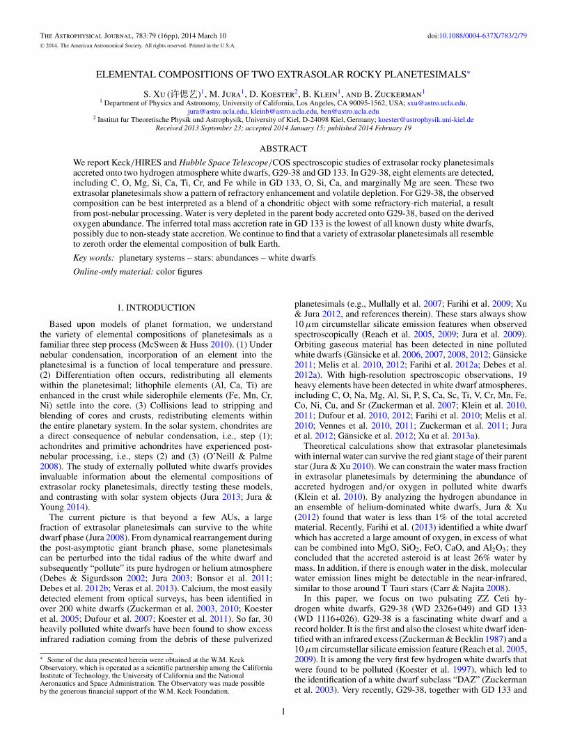
The carbon lines in the observed wavelength interval canbe contaminated by interstellar absorption because they arisefrom low lying energy levels. In a stellar environment, theC ii 1335.7 line is always stronger than the C ii 1334.5 line due toits larger statistical weight. However, as shown in Figure 3, theobserved C ii 1335.7 line is relatively weaker in both stars; weconclude that these C ii lines are mostly interstellar. In addition,the measured velocity for the C ii 1334.5 Å line is offset fromall other photospheric lines in G29-38 and GD 133. This linealso suffers from additional contamination from H2.

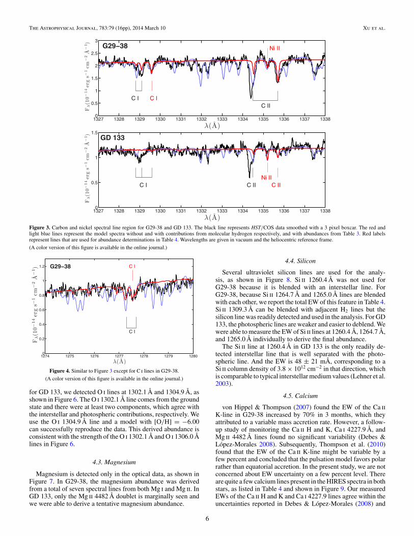
There are C i lines at 1277.6 Å and 1329.6 Å detected in G29-38, as shown in Figures 3 and 4. The detection is nominally atleast 5σ and, in the absence of H2, the derived abundance [C/H]would be −6.90 ± 0.08. However, due to their proximity to H2lines, the EW of the C i lines are less certain and we assign aconservative final abundance of -6.90 ± 0.12. For GD 133, theC ii line at 1335.7 Å was used to place the upper limit, which isconsistent with the upper bound from the C i 1329.6 Å line inFigure 3.

4.2. Oxygen

As presented in Figure 5, we have detected O i 1152.2 Å inG29-38, which can be reproduced by a model with an oxygenabundance of −5.00. The upper bound from O i triplet linesaround 7775 Å also agrees with this result.

In the wavelength coverage of COS, there are several O i linesaround 1300 Å, which can be contaminated from geocoronalemissions. When extracting the night time portions of the data

6 According to the dynamical model of the local interstellar medium:http://lism.wesleyan.edu/LISMdynamics.html.

4

The Astrophysical Journal, 783:79 (16pp), 2014 March 10 Xu et al.

Table 4Measured Equivalent Widths of Photospheric Lines and Abundance Determinations

Ion λa Elow log gf G29-38 GD 133

(Å) (eV) EW [Z/H] EW [Z/H](mÅ) (mÅ)

C i 1277.6 0.01 −0.40 52 ± 9H2 b −6.96 ± 0.08 · · · · · ·C i 1329.6 0.01 −0.62 42 ± 8H2 b −6.85 ± 0.08 · · · · · ·C ii 1335.7 0.01 −0.34 · · · · · · <20H2 b <−7.9C −6.90 ± 0.12 <−7.9

N i 1411.9 3.58 −1.3 <27 <−5.7 <25 <−5.8

O i 1152.2 1.97 −0.27 81 ± 22H2 b −5.00 ± 0.12 · · · · · ·O i 1304.9 0.02 −0.84 · · · · · · 63 ± 16 −6.00 ± 0.11O −5.00 ± 0.12 −6.00 ± 0.11

Na i 5891.6 0 0.12 <24 <−6.7 <30 <−6.3

Mg i 3830.4 2.71 −0.23 14 ± 3 −5.62 ± 0.09 · · · · · ·Mg i 3833 2.71 0.12, −0.36 21± 5 −5.89 ± 0.10 · · · · · ·Mg i 3839.4 2.72 0.39 35 ± 4 −5.86 ± 0.05 · · · · · ·Mg i 5174.1 2.71 −0.39 31 ± 4 −5.65 ± 0.06 · · · · · ·Mg i 5185.0 2.71 −0.17 42 ± 4 −5.72 ± 0.04 · · · · · ·Mg ii 4482 8.86 0.74, 0.59 41 ± 7 −5.91 ± 0.08 14 ± 4 −6.5:Mg −5.77 ± 0.13 · · · −6.5:

Al i 3945.1 0 −0.62 <16 <−6.1 <19 <−5.7

Si ii 1260.4 0 0.387 · · · · · · 93 ± 26 −6.67 ± 0.11Si ii 1264.7 0.04 0.64 320 ± 64Si iib −5.76 ± 0.09 115 ± 20 −6.70 ± 0.07Si ii 1265.0 0.04 −0.33 320 ± 64Si iib −5.76 ± 0.09 51 ± 12 −6.60 ± 0.13Si ii 1309.3 0.04 −0.43 106 ± 11H2 b −5.48 ± 0.05 61 ± 12H2 b −6.42 ± 0.05Si −5.60 ± 0.17 −6.60 ± 0.13

S i 1425.0 0 −0.12 <55H2 b <−7.0 <38H2 b <−7.0

Ca i 4227.9 0 0.27 17 ± 3 −6.67 ± 0.07 · · · · · ·Ca ii 3159.8 3.12 0.24 67 ± 5 −6.69 ± 0.03 · · · · · ·Ca ii 3180.3 3.15 0.50 109 ± 5 −6.61 ± 0.02 37 ± 4 −7.23 ± 0.05Ca ii 3182.2 3.15 −0.46 40 ± 4 −6.46 ± 0.04 · · · · · ·Ca ii 3707.1 3.12 −0.48 24 ± 4 −6.65 ± 0.07 · · · · · ·Ca ii 3934.8 0 0.11 294 ± 6 −6.65 ± 0.01 154 ± 13 −7.08 ± 0.04Ca ii 3969.6 0 −0.2 78± 7 −6.58 ± 0.04 27 ± 6 −7.07 ± 0.09Ca ii 8500.4 1.69 −1.4 84 ± 6 −6.34 ± 0.03 · · · · · ·Ca ii 8544.4 1.69 −0.46 185 ± 16 −6.54 ± 0.04 42 ± 7 −7.33 ± 0.07Ca ii 8664.5 1.69 −0.72 No Data No Data 28 ± 4 −7.34 ± 0.07Ca −6.58 ± 0.12 −7.21 ± 0.13

Ti ii 3235.4 0.05 0.43 13 ± 2 −8.06 ± 0.06 · · · · · ·Ti ii 3237.5 0.03 0.24 16 ± 6 −7.88 ± 0.15 · · · · · ·Ti ii 3350 0.61, 0.05 0.43, 0.53 31 ± 4 −7.95 ± 0.05 · · · · · ·Ti ii 3362.2 0.03 0.43 11± 2 −8.12 ± 0.08 <12 <−8.0Ti ii 3373.8 0.01 0.28 19 ± 3 −7.79 ± 0.05 · · · · · ·Ti ii 3384.7 0 0.16 19 ± 4 −7.70 ± 0.09 · · · · · ·Ti ii 3686.3 0.61 0.13 11± 2 −7.87 ± 0.08 · · · · · ·Ti −7.90 ± 0.16 · · · <−8.0

Cr ii 3125.9 2.46 0.30 13 ± 4 −7.42 ± 0.11 No Data No DataCr ii 3133.0 2.48 0.42 10± 4 −7.61 ± 0.17 No Data No DataCr ii 3369.0 2.48 −0.09 · · · · · · <14 <−6.8Cr −7.51 ± 0.12 <−6.8

Mn ii 3443.0 1.78 −0.36 <14 <−7.2 <15 <−7.0

Fe i 3582.2 0.86 0.41 12 ± 2 −5.97 ± 0.06 · · · · · ·Fe i 3735.9 0.86 0.32 13 ± 3 −5.82 ± 0.09 · · · · · ·Fe ii 1361.4 1.67 −0.52 · · · · · · <17 <−5.9Fe ii 3228.7 1.67 −1.18 12 ± 3 −5.79 ± 0.09 · · · · · ·Fe −5.90 ± 0.10 <−5.9

Ni ii 1335.2 0.19 −0.19 <20H2 b <−7.3 <24H2 b <−7.0

Notes. The adopted abundances are also presented in Table 3.a Wavelengths are in vacuum. Atomic data for absorption lines are taken from the Vienna Atomic Line Database(Kupka et al. 1999).b Blended line. The contributing element is noted in the superscript and the EW is the sum of the blend.

5

The Astrophysical Journal, 783:79 (16pp), 2014 March 10 Xu et al.

1327 1328 1329 1330 1331 1332 1333 1334 1335 1336 1337 13380

0.5

1

1.5

2

2.5

3G29−38

λ(A)

Fλ(1

0−14

erg

s−1

cm−

2A

−1)

C I C IC II

Ni II

1327 1328 1329 1330 1331 1332 1333 1334 1335 1336 1337 13380

0.5

1

1.5GD 133

λ(A)

Fλ(1

0−14

erg

s−1

cm−

2A

−1)

C I C II C IINi II

Figure 3. Carbon and nickel spectral line region for G29-38 and GD 133. The black line represents HST/COS data smoothed with a 3 pixel boxcar. The red andlight blue lines represent the model spectra without and with contributions from molecular hydrogen respectively, and with abundances from Table 3. Red labelsrepresent lines that are used for abundance determinations in Table 4. Wavelengths are given in vacuum and the heliocentric reference frame.

(A color version of this figure is available in the online journal.)

1274 1275 1276 1277 1278 1279 12800

0.2

0.4

0.6

0.8

1

1.2 G29−38

λ(A)

Fλ(1

0−14

erg

s−1

cm−

2A

−1) C I

C I

Figure 4. Similar to Figure 3 except for C i lines in G29-38.

(A color version of this figure is available in the online journal.)

for GD 133, we detected O i lines at 1302.1 Å and 1304.9 Å, asshown in Figure 6. The O i 1302.1 Å line comes from the groundstate and there were at least two components, which agree withthe interstellar and photospheric contributions, respectively. Weuse the O i 1304.9 Å line and a model with [O/H] = −6.00can successfully reproduce the data. This derived abundance isconsistent with the strength of the O i 1302.1 Å and O i 1306.0 Ålines in Figure 6.

4.3. Magnesium

Magnesium is detected only in the optical data, as shown inFigure 7. In G29-38, the magnesium abundance was derivedfrom a total of seven spectral lines from both Mg i and Mg ii. InGD 133, only the Mg ii 4482 Å doublet is marginally seen andwe were able to derive a tentative magnesium abundance.

4.4. Silicon

Several ultraviolet silicon lines are used for the analy-sis, as shown in Figure 8. Si ii 1260.4 Å was not used forG29-38 because it is blended with an interstellar line. ForG29-38, because Si ii 1264.7 Å and 1265.0 Å lines are blendedwith each other, we report the total EW of this feature in Table 4.Si ii 1309.3 Å can be blended with adjacent H2 lines but thesilicon line was readily detected and used in the analysis. For GD133, the photospheric lines are weaker and easier to deblend. Wewere able to measure the EW of Si ii lines at 1260.4 Å, 1264.7 Å,and 1265.0 Å individually to derive the final abundance.

The Si ii line at 1260.4 Å in GD 133 is the only readily de-tected interstellar line that is well separated with the photo-spheric line. And the EW is 48 ± 21 mÅ, corresponding to aSi ii column density of 3.8 × 1012 cm−2 in that direction, whichis comparable to typical interstellar medium values (Lehner et al.2003).

4.5. Calcium

von Hippel & Thompson (2007) found the EW of the Ca iiK-line in G29-38 increased by 70% in 3 months, which theyattributed to a variable mass accretion rate. However, a follow-up study of monitoring the Ca ii H and K, Ca i 4227.9 Å, andMg ii 4482 Å lines found no significant variability (Debes &Lopez-Morales 2008). Subsequently, Thompson et al. (2010)found that the EW of the Ca ii K-line might be variable by afew percent and concluded that the pulsation model favors polarrather than equatorial accretion. In the present study, we are notconcerned about EW uncertainty on a few percent level. Thereare quite a few calcium lines present in the HIRES spectra in bothstars, as listed in Table 4 and shown in Figure 9. Our measuredEWs of the Ca ii H and K and Ca i 4227.9 lines agree within theuncertainties reported in Debes & Lopez-Morales (2008) and

6

The Astrophysical Journal, 783:79 (16pp), 2014 March 10 Xu et al.

1150.5 1151 1151.5 1152 1152.5 11530

0.1

0.2

0.3

0.4

0.5

0.6

0.7

0.8

0.9

1

G29−38

λ(A)

Fλ(1

0−14

erg

s−1

cm−

2A

−1)

O I

7770 7772 7774 7776 7778 7780 77820.95

0.96

0.97

0.98

0.99

1

1.01

1.02

1.03

1.04

1.05

G29−38

λ(A)

Rel

ativ

eIn

tens

ity

O I

Figure 5. Similar to Figure 3 except for the detection of O i in G29-38. The right panel shows Keck/HIRES data smoothed with a 3 pixel boxcar and the spectrum isnot flux calibrated. Only one model is plotted for the optical data, which are free from H2 contamination.

(A color version of this figure is available in the online journal.)

1301 1302 1303 1304 1305 1306 13070

0.1

0.2

0.3

0.4

0.5

0.6

0.7

0.8

0.9

1

GD 133

λ(A)

Fλ(1

0−14

erg

s−1

cm−

2A

−1)

O I

O I

Si II

Figure 6. Similar to Figure 3 except for the night time portions of COS data ofGD 133. The spectrum was smoothed with a 3 pixel boxcar.

(A color version of this figure is available in the online journal.)

Thompson et al. (2010). In GD 133, there are five Ca ii linesdetected and [Ca/H] = −7.21. We measured an EW of 154 ±13 mÅ for the Ca ii K-line, which lies within the uncertaintyof the EW of 135 mÅ from VLT/UVES data but the derivedabundance is different due to the updated model atmospherecalculations (Koester et al. 2005; Koester & Wilken 2006).

4.6. Titanium

Seven titanium lines were detected in the Keck/HIRESspectrum of G29-38 and three are displayed in Figure 10.Although most titanium lines have EWs smaller than 20 mÅ,they are readily detected due to the high S/N of the data. In GD133, the Ti ii 3362.2 Å line was used to derive the upper limit.

4.7. Chromium

In G29-38, there are two chromium lines at 3125.9 Å and3133.0 Å in the observed wavelength interval as shown inFigure 10. The detection of each individual line is marginalbut the presence of lines at two correct wavelengths makes theidentification more convincing. In GD 133, these two chromiumlines fall off the edge of echelle orders and the next strongestchromium line at 3369.0 Å was used to derive the upper limit.

4.8. Iron

Three optical iron lines are detected in G29-38 and two ofthem are presented in Figure 11. Iron is not detected in GD 133.Since molecular hydrogen does not significantly interfere nearthe Fe ii 1361.4 Å region in GD 133, we use the absence of thisstrong Fe line to derive an upper limit to the abundance.

4.9. Additional Upper Limits

Nitrogen, Sulfur, Nickel. The nitrogen triplet around 1200 Åis in the wing of Lyα and the S/N of the spectrum is verylow, making N i 1411.9 Å the best nitrogen line in our data set,as shown in Figure 12. To derive the sulfur upper limit, S i1425.03 Å was used and the fit is presented in Figure 13. Dueto the presence of adjacent molecular hydrogen lines, the sulfurupper limit is less constraining in G29-38 than in GD 133. Wealso used Ni ii 1335.2 Å to determine the upper limit as shownin Figure 3.

Sodium, Aluminum, Manganese. Optical spectral lines wereused to determine the upper limits for these elements. The detailsare listed in Table 4 and their spectra are not presented.

7

The Astrophysical Journal, 783:79 (16pp), 2014 March 10 Xu et al.

3820 3825 3830 3835 3840 3845 3850 38550.75

0.8

0.85

0.9

0.95

1

1.05

G29−38

λ(A)

Rel

ativ

eIn

tensi

ty

Mg I

Hη

4480 4481 4482 4483 4484 44850.9

0.95

1

1.05

G29−38

λ(A)

Rel

ativ

eIn

tensi

ty

Mg II

4480 4481 4482 4483 4484 44850.9

0.95

1

1.05

GD 133

λ(A)

Rel

ativ

eIn

tensi

ty

Mg II

Figure 7. Similar to Figure 3 except for magnesium lines in the Keck spectra for G29-38 and GD 133. The spectrum in the top panel was smoothed with a 7 pixelboxcar while the ones in the lower panels are averaged by a 3 pixel boxcar. The fit to Hη in G29-38 is not ideal (see discussion in Section 3.1) but we were still able todirectly compare the EWs of Mg i lines in the data with the model. Detection of Mg in GD 133 is marginal.

(A color version of this figure is available in the online journal.)

1258 1259 1260 1261 1262 1263 1264 1265 1266 12670

0.2

0.4

0.6

0.8

1

G29−38

λ(A)

Fλ(1

0−14

erg

s−1

cm−

2A

−1)

Si II Si II

1258 1259 1260 1261 1262 1263 1264 1265 1266 12670

0.1

0.2

0.3

0.4

GD 133

λ(A)

Fλ(1

0−14

erg

s−1

cm−

2A

−1)

Si II

Figure 8. Similar to Figure 3 except for silicon lines. The Si ii line at 1260.4 Å comes from the ground state and can be only used for the analysis of GD 133 becauseit is well separated from the interstellar absorption line.

(A color version of this figure is available in the online journal.)

5. DISCUSSION

We have determined the abundances of eight elements inG29-38, including C, O, Mg, Si, Ca, Ti, Cr, Fe and placed

stringent upper limits on S and Ni. There are only threehydrogen-dominated white dwarfs with more than 8 elementsdetermined, i.e., 11 for WD 1929+012, 10 for WD 0843+516(Gansicke et al. 2012), and 9 for NLTT 43806 (Zuckerman et al.

8

The Astrophysical Journal, 783:79 (16pp), 2014 March 10 Xu et al.

3178 3179 3180 3181 3182 31830.6

0.7

0.8

0.9

1

1.1

G29−38

λ(A)

Rel

ativ

eIn

tensi

ty

Ca II

3932 3933 3934 3935 3936 3937 3938

0.5

0.6

0.7

0.8

0.9

1

1.1

G29−38

λ(A)

Rel

ativ

eIn

tensi

ty

Ca II

3178 3179 3180 3181 3182 31830.6

0.7

0.8

0.9

1

1.1

GD 133

λ(A)

Rel

ativ

eIn

tensi

ty

Ca II

3932 3933 3934 3935 3936 3937 3938

0.5

0.6

0.7

0.8

0.9

1

1.1

GD 133

λ(A)

Rel

ativ

eIn

tensi

ty

Ca II

Figure 9. Similar to Figure 3 except for calcium lines in the Keck/HIRES data. All spectra were smoothed by a five-point boxcar average.

(A color version of this figure is available in the online journal.)

3360 3365 3370 3375 3380 33850.9

0.95

1

1.05

G29−38

λ(A)

Rel

ativ

eIn

tensi

ty

Ti II

3120 3122 3124 3126 3128 3130 3132 3134 3136 3138 31400.9

0.95

1

1.05

1.1

G29−38

λ(A)

Rel

ativ

eIn

tensi

ty

Cr II

Figure 10. Similar to Figure 3 except for titanium and chromium lines. Both spectra were smoothed by a seven-point boxcar average.

(A color version of this figure is available in the online journal.)

2011). In GD 133, we have detected O, Si, and Ca, marginallydetected Mg, and placed a meaningful upper limit on the carbonabundance.

Both G29-38 and GD 133 show excess infrared radiationcoming from an orbiting dust disk (Zuckerman & Becklin 1987;Reach et al. 2005, 2009; Jura et al. 2007). The source of accretion

in both G29-38 and GD 133 is likely to come from one largeparent body rather than a blend of several small ones, mainlybecause collisions among different objects will evaporate all thedust particles and destroy the dust disk (Jura 2008). Because thesettling times of heavy elements in these white dwarfs are lessthan a year (Koester 2009), much shorter than the disk lifetime

9

The Astrophysical Journal, 783:79 (16pp), 2014 March 10 Xu et al.

3226 3227 3228 3229 3230 32310.95

0.96

0.97

0.98

0.99

1

1.01

1.02

1.03

1.04

1.05

G29−38

λ(A)

Rel

ativ

eIn

tens

ity

Fe II

3734 3735 3736 3737 3738 3739 37400.85

0.9

0.95

1

1.05

G29−38

λ(A)R

elat

ive

Inte

nsit

y

Fe I Ca II + Fe I

Figure 11. Similar to Figure 3 except for iron lines in G29-38. Both spectra were smoothed by a five-point boxcar average. The absorption feature around 3738 Å is ablend of Ca ii and Fe i lines, which is dominated by Ca ii.

(A color version of this figure is available in the online journal.)

1409 1410 1411 1412 1413 14140

0.5

1

1.5

2

2.5

3

3.5

4

4.5

5

G29−38

λ(A)

Fλ(1

0−14

erg

s−1

cm−

2A

−1)

N I

Fe II

1409 1410 1411 1412 1413 14140

0.5

1

1.5

2

2.5

GD 133

λ(A)

Fλ(1

0−14

erg

s−1

cm−

2A

−1)

N I

Fe II

Figure 12. Similar to Figure 3 except for N i 1411.9 Å, which is used to derive nitrogen upper limits. Only a model without molecular hydrogen is shown and usedfor the analysis. All the unlabeled features in the data are from molecular hydrogen.

(A color version of this figure is available in the online journal.)

of ∼105 yr (Farihi et al. 2012b), the accretion is likely to bein a steady state, wherein the rate of material falling on thewhite dwarf atmosphere is balanced by the settling out of theconvection zone (Koester 2009). We can infer the compositionof the accreted extrasolar planetesimals based on the accretionflux, which is dependent on the settling times of each element.

5.1. Calculation of Settling Times

Very recently, Deal et al. (2013) have drawn attention tothe fingering or thermohaline instability; they find that this

effect is important in hydrogen-dominated white dwarfs andcan change the derived accretion rates by orders of magnitude.Unfortunately they do not publish enough details for us to drawconclusions about the relevance of the effect for the whitedwarfs studied here. Some problems we see in Deal et al.(2013) are:

1. Deal et al. (2013) use a prescription for the thermohalinediffusion coefficient from Vauclair & Theado (2012), whichis claimed to be physically more realistic than previousmethods. However, their formula leads to an infinite value

10

The Astrophysical Journal, 783:79 (16pp), 2014 March 10 Xu et al.

1423 1424 1425 1426 1427 14280

1

2

3

4

5

6

7

G29−38

λ(A)

Fλ(1

0−14

erg

s−1

cm−

2A

−1)

S I

1423 1424 1425 1426 1427 14280

0.5

1

1.5

2

2.5

3

3.5

GD 133

λ(A)F

λ(1

0−14

erg

s−1

cm−

2A

−1)

S I

Fe II

Figure 13. Similar to Figure 3 except for S i 1425.0 Å, which is used to derive sulfur upper limits.

(A color version of this figure is available in the online journal.)

for the coefficient at the bottom of the convection zone,which is unrealistic.

2. In our model for G29-38 the bottom of the convection zoneis at log (Mcvz/M∗) = −13.95 (see Table 2) and the layersabove this will be homogeneously mixed in a matter ofseconds. In Deal et al. (2013), the model 3 presented inboth Figure 1 and 2 has no convection at all. The model 2,with parameters closest to G29-38 has a convection zone afactor of 100 smaller than G29-38. None of these modelscan represent our current objects.

3. The H/He interface at log (Mcvz/M∗) = −5 is not a sharpboundary, but a transition zone. The helium will mix upwardinto the hydrogen and a significant helium fraction will stillbe present several pressure scale heights above this layer.This will lead to an increasing molecular weight, an effectapparently not considered in Deal et al. (2013).

4. Their main argument is the fact that in previous determina-tions the accretion rates for helium white dwarfs seemed tobe systematically higher than in hydrogen white dwarfs. Inour opinion, a much more likely reason is the uncertainty inthe depth of the convection zones in helium white dwarfs,which is described in corrected diffusion times7 as wellas possibly non-steady state accretion (see Section 5.3 formore discussion).

For the time being, we do not believe that the Deal et al.(2013) calculations are applicable to G29-38 or GD 133; butwe will reconsider our conclusions, once more details becomeavailable.

5.2. G29-38

The abundances in the parent body that accreted onto G29-38are calculated by correcting for the settling effect of each ele-ment in the atmosphere, as shown in Table 3. In addition, theabundances can also be derived by fitting the infrared spectrum

7 See www.astrophysik.uni-kiel.de/∼koester.

C O Si S Ca Fe−2.5

−2

−1.5

−1

−0.5

0

0.5

1

log

n(Z

)/n

(Mg)

Reach+2009This Work

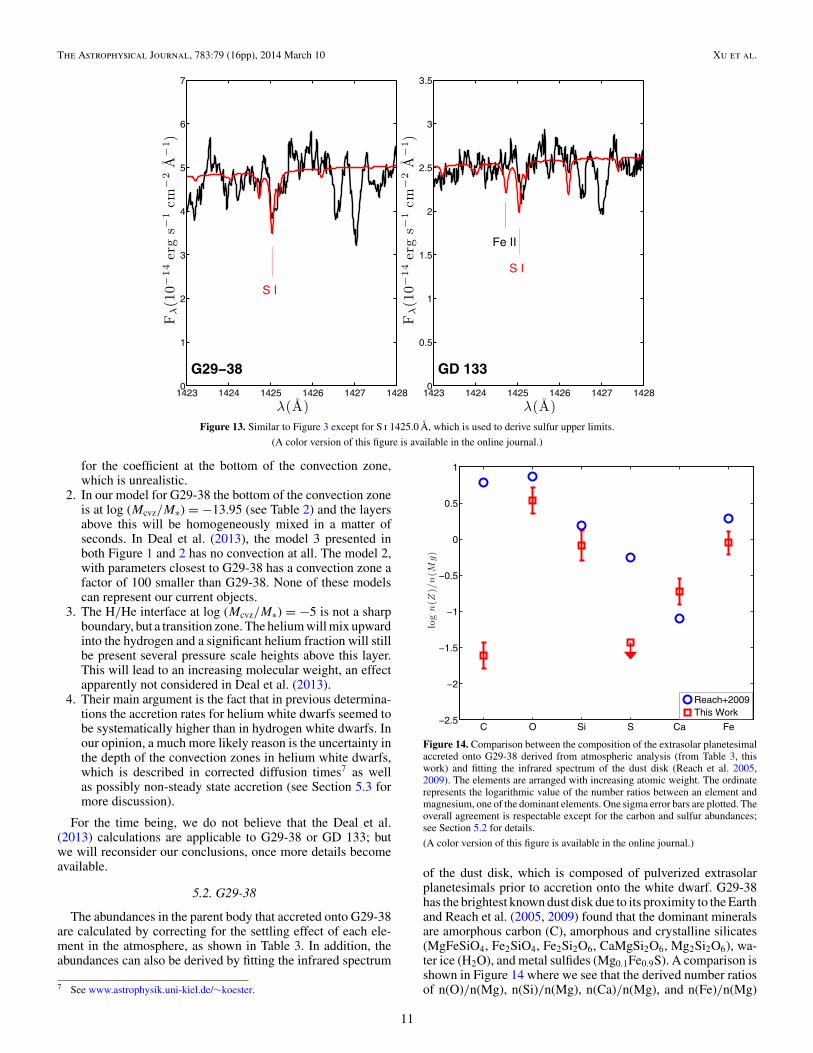
Figure 14. Comparison between the composition of the extrasolar planetesimalaccreted onto G29-38 derived from atmospheric analysis (from Table 3, thiswork) and fitting the infrared spectrum of the dust disk (Reach et al. 2005,2009). The elements are arranged with increasing atomic weight. The ordinaterepresents the logarithmic value of the number ratios between an element andmagnesium, one of the dominant elements. One sigma error bars are plotted. Theoverall agreement is respectable except for the carbon and sulfur abundances;see Section 5.2 for details.

(A color version of this figure is available in the online journal.)

of the dust disk, which is composed of pulverized extrasolarplanetesimals prior to accretion onto the white dwarf. G29-38has the brightest known dust disk due to its proximity to the Earthand Reach et al. (2005, 2009) found that the dominant mineralsare amorphous carbon (C), amorphous and crystalline silicates(MgFeSiO4, Fe2SiO4, Fe2Si2O6, CaMgSi2O6, Mg2Si2O6), wa-ter ice (H2O), and metal sulfides (Mg0.1Fe0.9S). A comparison isshown in Figure 14 where we see that the derived number ratiosof n(O)/n(Mg), n(Si)/n(Mg), n(Ca)/n(Mg), and n(Fe)/n(Mg)

11

The Astrophysical Journal, 783:79 (16pp), 2014 March 10 Xu et al.

0 1 2 3 4 5 6 7 8 9 10

χ2red[G29-38]

Carbonaceous ChondriteOrdinary ChondriteEnstatie ChondriteR ChondritePrimitive AchondriteAsteroidal MeteoriteLunar MeteoriteMartian MeteoritePallasiteMesosideriteBulk EarthTerrestrial RockH+HOW

0 1 2 3 4 5 6 7 8 9 10

χ2red[GD 133]

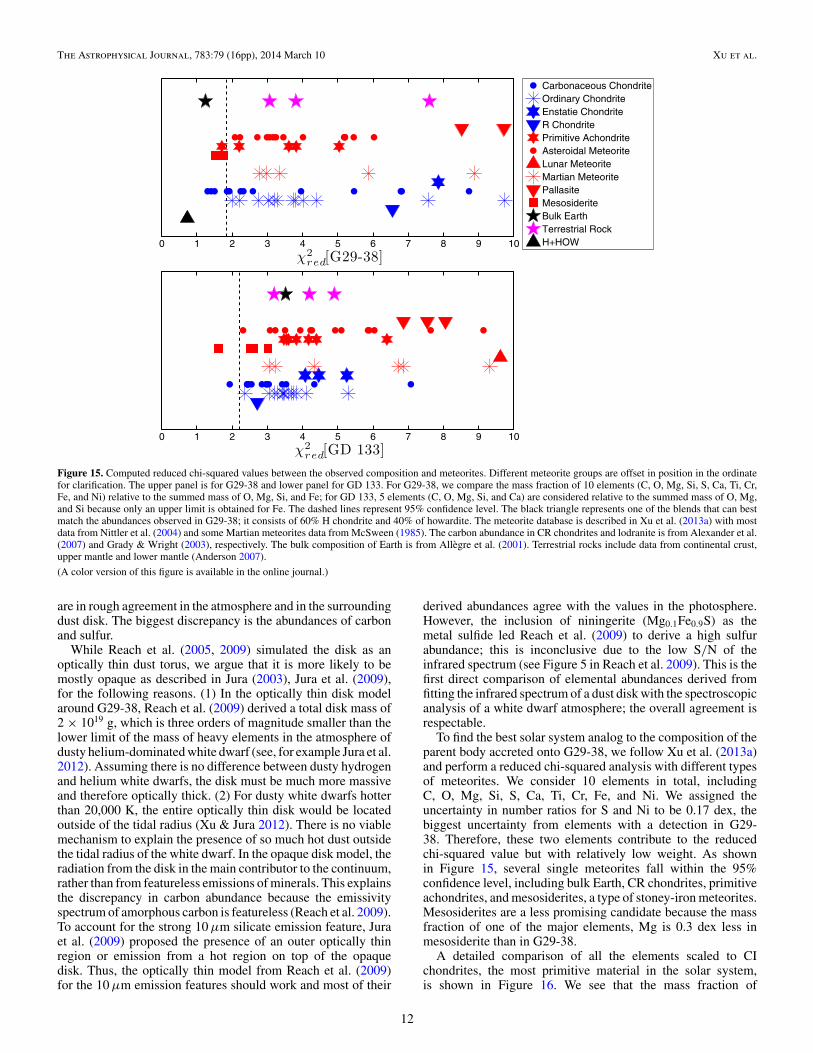
Figure 15. Computed reduced chi-squared values between the observed composition and meteorites. Different meteorite groups are offset in position in the ordinatefor clarification. The upper panel is for G29-38 and lower panel for GD 133. For G29-38, we compare the mass fraction of 10 elements (C, O, Mg, Si, S, Ca, Ti, Cr,Fe, and Ni) relative to the summed mass of O, Mg, Si, and Fe; for GD 133, 5 elements (C, O, Mg, Si, and Ca) are considered relative to the summed mass of O, Mg,and Si because only an upper limit is obtained for Fe. The dashed lines represent 95% confidence level. The black triangle represents one of the blends that can bestmatch the abundances observed in G29-38; it consists of 60% H chondrite and 40% of howardite. The meteorite database is described in Xu et al. (2013a) with mostdata from Nittler et al. (2004) and some Martian meteorites data from McSween (1985). The carbon abundance in CR chondrites and lodranite is from Alexander et al.(2007) and Grady & Wright (2003), respectively. The bulk composition of Earth is from Allegre et al. (2001). Terrestrial rocks include data from continental crust,upper mantle and lower mantle (Anderson 2007).

(A color version of this figure is available in the online journal.)

are in rough agreement in the atmosphere and in the surroundingdust disk. The biggest discrepancy is the abundances of carbonand sulfur.

While Reach et al. (2005, 2009) simulated the disk as anoptically thin dust torus, we argue that it is more likely to bemostly opaque as described in Jura (2003), Jura et al. (2009),for the following reasons. (1) In the optically thin disk modelaround G29-38, Reach et al. (2009) derived a total disk mass of2 × 1019 g, which is three orders of magnitude smaller than thelower limit of the mass of heavy elements in the atmosphere ofdusty helium-dominated white dwarf (see, for example Jura et al.2012). Assuming there is no difference between dusty hydrogenand helium white dwarfs, the disk must be much more massiveand therefore optically thick. (2) For dusty white dwarfs hotterthan 20,000 K, the entire optically thin disk would be locatedoutside of the tidal radius (Xu & Jura 2012). There is no viablemechanism to explain the presence of so much hot dust outsidethe tidal radius of the white dwarf. In the opaque disk model, theradiation from the disk in the main contributor to the continuum,rather than from featureless emissions of minerals. This explainsthe discrepancy in carbon abundance because the emissivityspectrum of amorphous carbon is featureless (Reach et al. 2009).To account for the strong 10 μm silicate emission feature, Juraet al. (2009) proposed the presence of an outer optically thinregion or emission from a hot region on top of the opaquedisk. Thus, the optically thin model from Reach et al. (2009)for the 10 μm emission features should work and most of their

derived abundances agree with the values in the photosphere.However, the inclusion of niningerite (Mg0.1Fe0.9S) as themetal sulfide led Reach et al. (2009) to derive a high sulfurabundance; this is inconclusive due to the low S/N of theinfrared spectrum (see Figure 5 in Reach et al. 2009). This is thefirst direct comparison of elemental abundances derived fromfitting the infrared spectrum of a dust disk with the spectroscopicanalysis of a white dwarf atmosphere; the overall agreement isrespectable.

To find the best solar system analog to the composition of theparent body accreted onto G29-38, we follow Xu et al. (2013a)and perform a reduced chi-squared analysis with different typesof meteorites. We consider 10 elements in total, includingC, O, Mg, Si, S, Ca, Ti, Cr, Fe, and Ni. We assigned theuncertainty in number ratios for S and Ni to be 0.17 dex, thebiggest uncertainty from elements with a detection in G29-38. Therefore, these two elements contribute to the reducedchi-squared value but with relatively low weight. As shownin Figure 15, several single meteorites fall within the 95%confidence level, including bulk Earth, CR chondrites, primitiveachondrites, and mesosiderites, a type of stoney-iron meteorites.Mesosiderites are a less promising candidate because the massfraction of one of the major elements, Mg is 0.3 dex less inmesosiderite than in G29-38.

A detailed comparison of all the elements scaled to CIchondrites, the most primitive material in the solar system,is shown in Figure 16. We see that the mass fraction of

12

The Astrophysical Journal, 783:79 (16pp), 2014 March 10 Xu et al.

C O S Cr Si Fe Mg Ni Ca Ti−1.5

−1

−0.5

0

0.5

1

log

f(Z

/(O

+M

g+

Si+

Fe))

f(Z

/(O

+M

g+

Si+

Fe))

CI

G29−38H+HOWBulk Earth

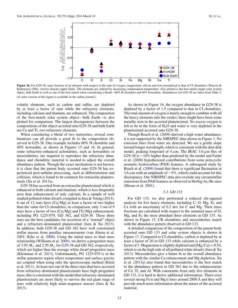
Figure 16. For G29-38, mass fraction of an element with respect to the sum of oxygen, magnesium, silicon and iron normalized to that of CI chondrites (Wasson &Kallemeyn 1988). Arrows denotes upper limits. The elements are ordered by increasing condensation temperature. Also plotted is the best match single solar systemobject, bulk Earth as well as one of the best match when considering a blend—60% H chondrite and 40% howadrite. Abundances for G29-38 are taken from Table 3.

(A color version of this figure is available in the online journal.)

volatile elements, such as carbon and sulfur, are depletedby at least a factor of nine while the refractory elements,including calcium and titanium, are enhanced. The compositionof the best-match solar system object—bulk Earth—is alsoplotted for comparison. The largest discrepancies between thecompositions of the object accreted onto G29-38 and bulk Earthare Ca and Ti, two refractory elements.

When considering a blend of two meteorites, several com-binations can all provide a good fit to the composition ob-served in G29-38. One example includes 60% H chondrite and40% howardite, as shown in Figures 15 and 16. In general,some refractory-enhanced achondrites, such as howardites ormesosiderites, are required to reproduce the refractory abun-dance and chondritic material is needed to adjust the overallabundance pattern. Though the exact mechanism is not known,it is clear that the parent body accreted onto G29-38 has ex-perienced post-nebular processing, such as differentiation andcollision, which is found to be common for extrasolar planetes-imals (Xu et al. 2013a).

G29-38 has accreted from an extrasolar planetesimal which isenhanced in both calcium and titanium, which is less frequentlyseen than enhancement of only calcium. In a sample of wellstudied polluted white dwarfs compiled in Jura & Young (2014),6 out of 12 stars have [Ca/Mg] at least a factor of two higherthan the value for CI chondrites; in comparison, only 3 out of 9stars have a factor of two [Ca/Mg] and [Ti/Mg] enhancement,including PG 1225-079, GD 362, and G29-38. These threestars are the best candidates for accretion of a “normal” objectand a refractory-dominated planetesimal (Jura & Xu 2013).In addition, both G29-38 and GD 362 have well constrainedstellar masses from parallax measurements (van Altena et al.2001; Kilic et al. 2008). Using the initial mass to final massrelationship (Williams et al. 2009), we derive a progenitor massof 3.95 M� and 2.95 M� for G29-38 and GD 362, respectively,which are higher than the average white dwarf progenitor mass(Kleinman et al. 2013). Unfortunately, PG 1225-079 is in thestellar parameter region where temperature and surface gravityare coupled when using only the spectroscopic method (Kleinet al. 2011). At least two out of the three stars that have accretedfrom refractory-dominated planetesimals have high progenitormass; this is consistent with the model that refractory-dominatedplanetesimals are more likely to survive the red giant stage ofstars with relatively high main-sequence masses (Jura & Xu2013).

As shown in Figure 16, the oxygen abundance in G29-38 isdepleted by a factor of 1.5 compared to that in CI chondrites.The total amount of oxygen is barely enough to combine with allthe heavy elements into the oxides; there might have been somemetallic iron in the accreted planetesimal. No excess oxygen isleft to be in the form of H2O and water is very depleted in theplanetesimal accreted onto G29-38.

Though Reach et al. (2009) derived a high water abundance,it is not supported by the NIRSPEC data shown in Figure 1. Noemission lines from water are detected. We see a gentle slopetoward longer wavelength, which is consistent with the dust diskmodel, peaking longward of 4 μm. The IRAC 3.6 μm flux ofG29-38 is ∼10% higher than predicted by the model and Farihiet al. (2008) hypothesized contributions from some polycyclicaromatic hydrocarbon (PAH) features. A subsequent study byReach et al. (2009) found that there is significant fluctuation at3.6 μm with an amplitude of ∼5%, which could account for thisdiscrepancy. Our NIRSPEC data also exclude any circumstellaremissions from PAH features as observed in Herbig Ae/Be stars(Meeus et al. 2001).

5.3. GD 133

For GD 133, we also performed a reduced chi-squaredanalysis for five heavy elements, including C, O, Mg, Si, andCa with an uncertainty of 0.2 dex for C and Mg. Their massfractions are calculated with respect to the summed mass of O,Mg, and Si, the most abundant three elements in GD 133. Asshown in Figure 15, CR chondrites and mesosiderites matchwith the abundance pattern observed in GD 133.

A detailed comparison of the composition of the parent bodyaccreted onto GD 133 and solar system objects is shown inFigure 17. Compared to CI chondrites, carbon is depleted by atleast a factor of 20 in GD 133 while calcium is enhanced by afactor of 3. Magnesium is slightly depleted and [Mg/Ca] = 0.54,which is on the high side of all polluted white dwarfs (Jura & Xu2013). Mesosiderites give a better fit to the overall abundancepattern with the similar Ca enhancement and Mg depletion. Xuet al. (2013a) also found that mesosiderites is the best matchto the abundance pattern in GD 362 due to the enhancementsof Ca, Ti, and Al. With constraints from only five elements inGD 133, it is hard to derive additional information. There existseveral strong Fe ii and Mg ii lines around 2800 Å and they willprovide much more information about the nature of the accretedmaterial.

13

The Astrophysical Journal, 783:79 (16pp), 2014 March 10 Xu et al.

C O S Si Fe Mg Ca−1.5

−1

−0.5

0

0.5

1

log

f(Z

/O

+M

g+

Si)

f(Z

/O

+M

g+

Si)

CI

GD133MESCR

Figure 17. Similar to Figure 16 except for GD 133 and the mass fraction of an element normalized to the sum of oxygen, magnesium, and silicon. There is no error barassociated with magnesium because it is only marginally detected. The compositions of two best match meteorites from the reduced chi-squared analysis, mesosideriteand CR chondrite, are also plotted for comparison.

(A color version of this figure is available in the online journal.)

Figure 18. Compilation of all polluted white dwarfs with detections of at least O, Mg, Si, and Fe; eight of these stars also have good constraints on the carbonabundance. The abscissa marks white dwarf effective temperatures, corresponding to a cooling age less than 500 Myr; the ordinate is surface gravity, which showsa main-sequence mass between 1.8–4.0 M� for the current sample. For clarity, some objects are slightly offset in their plotted positions. The abundances have beencorrected for the effect of settling and we only show the mass fraction of O, Mg, Si, and Fe; the rest are left blank. The size of a pie correlates with the accretionrate (not to scale). We see that O, Mg, Si, and Fe are always the dominant elements in a variety of extrasolar planetesimals, resembling bulk Earth. No carbon richplanetesimals similar to comet Halley have been identified so far. The white dwarfs are ordered with increasing stellar temperatures. References: Hydrogen-dominatedwhite dwarfs: 1: G29-38 (this paper), 7: PG 1015+161, 8: WD 1226+110, 9: WD 1929+012, 10: WD 0843+516 (Gansicke et al. 2012); helium-dominated whitedwarfs: 2: WD J0738+1835 (Dufour et al. 2012), 3: HS 2253+8023 (Klein et al. 2011), 4: G241-6, 5: GD 40 (Jura et al. 2012), 6: GD 61 (Farihi et al. 2011, 2013).All white dwarfs except 3 and 4 have a dust disk. Bulk Earth: Allegre et al. (2001). Comet Halley: Jessberger et al. (1988).

(A color version of this figure is available in the online journal.)

Until now, all dusty white dwarfs are heavily polluted withmass accretion rates of at least 1 × 108 g s−1 (Farihi et al.2009; Brinkworth et al. 2012). GD 133 has a dust disk, whichreprocesses about 0.5% of the incoming star light (Jura et al.2007; Farihi et al. 2010). Assuming a chondritic iron to siliconratio, the accretion rate of iron is 5.9 × 106 g s−1 and the totalaccretion rate is 3.0 × 107 g s−1, the lowest of all dusty whitedwarfs. Even with an iron abundance of [Fe/H] = −5.9 (theupper limit listed in Table 3), the total accretion rate can onlyadd up to 7.6 × 107 g s−1, marginally lower than all other dusty

white dwarfs. In a steady state model, Poynting–Robertson dragprovides a lower bound of the accretion rate (Rafikov 2011; Xu& Jura 2012):

M = 16φr

3

r3∗

rin

σT 4eff

c2, (1)

φr is an efficiency coefficient and taken as 1. σ and c are theStephan–Boltzman constant and the speed of light, respectively.For GD 133, the stellar temperature Teff is listed in Table 2and the stellar radius r∗ = 0.012r�. Depending on the disk

14

The Astrophysical Journal, 783:79 (16pp), 2014 March 10 Xu et al.

inclination, the inner radius of the disk can vary (Jura et al.2007). To derive a lower limit of the mass accretion rate, wetake the largest possible inner radius rin = 23r∗ for a nearlyface-on disk, and consequently M = 2.5 × 108 g s−1, aboutan order of magnitude higher than the most likely inferredvalue. The exceptionally low accretion rate in GD 133 providesdirect evidence that Equation (1) does not always hold, possiblybecause the accretion process onto the star is not always in asteady state.

There exists additional evidence for time-varying non-steadystate accretion. Based on the different accretion rates derivedfrom hydrogen and helium atmosphere white dwarfs, Farihi et al.(2012b) postulated a non-steady state accretion model includinga high accretion stage and a low accretion stage. Now with anupdated helium model atmosphere and settling times (Xu et al.2013a), the difference has narrowed but is still present.

6. PERSPECTIVE

So far, there are 10 white dwarfs that have detections ofat least O, Mg, Si, and Fe in the atmosphere. As presentedin Figure 18, they are sampled from a variety of stellartemperatures and surface gravity. Five of these stars havea hydrogen-dominated atmosphere and five of them have ahelium-dominated atmosphere. Eight stars also have a dustdisk. Yet, to zeroth order, the resemblance of their elementalcompositions relative to bulk Earth is robust. No carbon richextrasolar planetesimals, e.g., analogs to comet Halley with 28%carbon (Jessberger et al. 1988) or interplanteary dust particlewith ∼10% carbon (Thomas et al. 1993), are identified inthe current sample. The only white dwarf that has accretedobjects with a considerable amount of water is GD 61 (6 inthe plot), which contains 26% water by mass (Farihi et al.2013). The general properties of extrasolar planetesimals can besummarized as the following (Jura & Young 2014), (1) oxygen,iron, silicon, and magnesium always dominate and make upmore than 85% of the total mass; (2) carbon is always depletedrelative to the solar abundance; and (3) viewed as an ensemble,water is less than 1% of the total accreted mass but exceptionsexist. As shown in Figure 18, there are variations among theabundances of different elements but they are only a factorof 2–3, comparable to the errors. To move beyond a zerothorder result, one must determine abundances of as many traceelements as possible, such as the case of GD 362 (Zuckermanet al. 2007; Xu et al. 2013a). Alternatively, one can assess theabundances of a few elements in an ensemble of stars, e.g., Jura& Xu (2012, 2013).

7. CONCLUSIONS

In this paper, we report optical and ultraviolet spectroscopicstudies of two externally polluted hydrogen-dominated whitedwarfs, G29-38 and GD 133. For G29-38, with the exceptionof carbon and sulfur, the derived elemental abundances agreereasonably well with the values obtained from fitting the infraredspectrum of the dust disk. Both stars have accreted objects thatshow a pattern of volatile depletion and refractory enhancement.The parent body accreted onto G29-38 has experienced post-nebular processing and can be best explained by a blend ofchrondritic material and a refractory-enhanced object. The totalmass accretion rate in GD 133 is significantly lower than all otherdusty white dwarfs, suggesting non-steady state accretion. In asample of 10 stars, we find that the elemental compositions of

extrasolar planetesimals are similar to bulk Earth regardless oftheir evolutionary history.

We thank G. Mace for helping with the NIRSPEC observingrun and useful discussions about data reduction procedures, C.Melis for helping with HIRES observing runs in 2008, andB. Holden for useful email exchanges regarding the MAKEEsoftware. Support for program no. 12290 was provided byNASA through a grant from the Space Telescope ScienceInstitute, which is operated by the Association of Universitiesfor Research in Astronomy, Inc., under NASA contract NAS5-26555. The authors wish to recognize and acknowledge thevery significant cultural role and reverence that the summit ofMauna Kea has always had within the indigenous Hawaiiancommunity. We are most fortunate to have the opportunity toconduct observations from this mountain. This work has beenpartly supported by NSF & NASA grants to UCLA to studypolluted white dwarfs.

REFERENCES

Alexander, C. M. O., Fogel, M., Yabuta, H., & Cody, G. D. 2007, GeCoA,71, 4380

Allegre, C., Manhes, G., & Lewin, E. 2001, E&PS, 185, 49Anderson, D. 2007, New Theory of the Earth (Cambridge: Cambridge Univ.

Press)Bonsor, A., Mustill, A. J., & Wyatt, M. C. 2011, MNRAS, 414, 930Brinkworth, C. S., Gansicke, B. T., Girven, J. M., et al. 2012, ApJ, 750, 86Carr, J. S., & Najita, J. R. 2008, Sci, 319, 1504Chen, Y.-H., & Li, Y. 2013, RAA, 13, 1438Deal, M., Deheuvels, S., Vauclair, G., Vauclair, S., & Wachlin, F. C. 2013, A&A,

557, L12Debes, J. H., Kilic, M., Faedi, F., et al. 2012a, ApJ, 754, 59Debes, J. H., & Lopez-Morales, M. 2008, ApJL, 677, L43Debes, J. H., & Sigurdsson, S. 2002, ApJ, 572, 556Debes, J. H., Walsh, K. J., & Stark, C. 2012b, ApJ, 747, 148Dufour, P., Bergeron, P., Liebert, J., et al. 2007, ApJ, 663, 1291Dufour, P., Kilic, M., Fontaine, G., et al. 2010, ApJ, 719, 803Dufour, P., Kilic, M., Fontaine, G., et al. 2012, ApJ, 749, 6Farihi, J., Becklin, E. E., & Zuckerman, B. 2008, ApJ, 681, 1470Farihi, J., Brinkworth, C. S., Gansicke, B. T., et al. 2011, ApJL, 728, L8Farihi, J., Gansicke, B. T., & Koester, D. 2013, Sci, 342, 218Farihi, J., Gansicke, B. T., Steele, P. R., et al. 2012a, MNRAS, 421, 1635Farihi, J., Gansicke, B. T., Wyatt, M. C., et al. 2012b, MNRAS, 424, 464Farihi, J., Jura, M., Lee, J., & Zuckerman, B. 2010, ApJ, 714, 1386Farihi, J., Jura, M., & Zuckerman, B. 2009, ApJ, 694, 805Gansicke, B. T. 2011, in AIP Conf. Ser. 1331, Planetary Systems beyond the

Main Sequence, ed. S. Schuh, H. Drechsel, & U. Heber (Melville, NY: AIP),211

Gansicke, B. T., Koester, D., Farihi, J., et al. 2012, MNRAS, 424, 333Gansicke, B. T., Koester, D., Marsh, T. R., Rebassa-Mansergas, A., &

Southworth, J. 2008, MNRAS, 391, L103Gansicke, B. T., Marsh, T. R., & Southworth, J. 2007, MNRAS, 380, L35Gansicke, B. T., Marsh, T. R., Southworth, J., & Rebassa-Mansergas, A.

2006, Sci, 314, 1908Giammichele, N., Bergeron, P., & Dufour, P. 2012, ApJS, 199, 29Gianninas, A., Bergeron, P., & Ruiz, M. T. 2011, ApJ, 743, 138Grady, M. M., & Wright, I. P. 2003, SSRv, 106, 231Holberg, J. B., Bergeron, P., & Gianninas, A. 2008, AJ, 135, 1239Hummer, D. G., & Mihalas, D. 1988, ApJ, 331, 794Jessberger, E. K., Christoforidis, A., & Kissel, J. 1988, Natur, 332, 691Jura, M. 2003, ApJL, 584, L91Jura, M. 2008, AJ, 135, 1785Jura, M. 2013, arXiv:1301.5562Jura, M., Farihi, J., & Zuckerman, B. 2007, ApJ, 663, 1285Jura, M., Farihi, J., & Zuckerman, B. 2009, AJ, 137, 3191Jura, M., & Xu, S. 2010, AJ, 140, 1129Jura, M., & Xu, S. 2012, AJ, 143, 6Jura, M., & Xu, S. 2013, AJ, 145, 30Jura, M., Xu, S., Klein, B., Koester, D., & Zuckerman, B. 2012, ApJ, 750, 69Jura, M., & Young, E. D. 2014, AREPS, 42Kilic, M., Thorstensen, J. R., & Koester, D. 2008, ApJL, 689, L45Klein, B., Jura, M., Koester, D., & Zuckerman, B. 2011, ApJ, 741, 64

15

The Astrophysical Journal, 783:79 (16pp), 2014 March 10 Xu et al.

Klein, B., Jura, M., Koester, D., Zuckerman, B., & Melis, C. 2010, ApJ,709, 950

Kleinman, S. J., Kepler, S. O., Koester, D., et al. 2013, ApJS, 204, 5Koester, D. 2009, A&A, 498, 517Koester, D. 2010, MmSAI, 81, 921Koester, D., Girven, J., Gansicke, B. T., & Dufour, P. 2011, A&A, 530, A114Koester, D., & Kompa, E. 2007, A&A, 473, 239Koester, D., Provencal, J., & Shipman, H. L. 1997, A&A, 320, L57Koester, D., Rollenhagen, K., Napiwotzki, R., et al. 2005, A&A, 432, 1025Koester, D., & Wilken, D. 2006, A&A, 453, 1051Kriss, G. A. 2011, Improved Medium Resolution Line Spread Functions for COS

FUV Spectra, Technical Report, http://www.stsci.edu/hst/cos/documents/isrs/ISR2011_01.pdf

Kupka, F., Piskunov, N., Ryabchikova, T. A., Stempels, H. C., & Weiss, W. W.1999, A&AS, 138, 119

Lehner, N., Jenkins, E. B., Gry, C., et al. 2003, ApJ, 595, 858McLean, I. S., Becklin, E. E., Bendiksen, O., et al. 1998, Proc. SPIE, 3354, 566McLean, I. S., Graham, J. R., Becklin, E. E., et al. 2000, Proc. SPIE, 4008, 1048McLean, I. S., McGovern, M. R., Burgasser, A. J., et al. 2003, ApJ, 596, 561McSween, H. Y. 1985, RvGeo, 23, 391McSween, H. Y., & Huss, G. R. 2010, Cosmochemistry (Cambridge: Cambridge

Univ. Press)Meeus, G., Waters, L. B. F. M., Bouwman, J., et al. 2001, A&A, 365, 476Melis, C., Dufour, P., Farihi, J., et al. 2012, ApJL, 751, L4Melis, C., Jura, M., Albert, L., Klein, B., & Zuckerman, B. 2010, ApJ,

722, 1078Mullally, F., Kilic, M., Reach, W. T., et al. 2007, ApJS, 171, 206Nittler, L. R., McCoy, T. J., Clark, P. E., et al. 2004, AMR, 17, 231O’Neill, H. S. C., & Palme, H. 2008, RSPTA, 366, 4205Rafikov, R. R. 2011, ApJL, 732, L3Reach, W. T., Lisse, C., von Hippel, T., & Mullally, F. 2009, ApJ, 693, 697

Reach, W. T., Megeath, S. T., Cohen, M., et al. 2005, PASP, 117, 978Redfield, S., & Linsky, J. L. 2008, ApJ, 673, 283Thomas, K. L., Blanford, G. E., Keller, L. P., Klock, W., & McKay, D. S.

1993, GeCoA, 57, 1551Thompson, S. E., Montgomery, M. H., von Hippel, T., et al. 2010, ApJ,

714, 296Tokunaga, A. T., Becklin, E. E., & Zuckerman, B. 1990, ApJL, 358, L21Tremblay, P.-E., & Bergeron, P. 2009, ApJ, 696, 1755Tremblay, P.-E., Bergeron, P., Kalirai, J. S., & Gianninas, A. 2010, ApJ,

712, 1345van Altena, W. F., Lee, J. T., & Hoffleit, E. D. 2001, yCat, 1238, 0Vauclair, S., & Theado, S. 2012, ApJ, 753, 49Vennes, S., Kawka, A., & Nemeth, P. 2010, MNRAS, 404, L40Vennes, S., Kawka, A., & Nemeth, P. 2011, MNRAS, 413, 2545Veras, D., Mustill, A. J., Bonsor, A., & Wyatt, M. C. 2013, MNRAS, 431,

1686Vogt, S. S., Allen, S. L., Bigelow, B. C., et al. 1994, Proc. SPIE, 2198, 362von Hippel, T., & Thompson, S. E. 2007, ApJ, 661, 477Wasson, J. T., & Kallemeyn, G. W. 1988, RSPTA, 325, 535Williams, K. A., Bolte, M., & Koester, D. 2009, ApJ, 693, 355Xu, S., & Jura, M. 2012, ApJ, 745, 88Xu, S., Jura, M., Klein, B., Koester, D., & Zuckerman, B. 2013a, ApJ, 766, 132Xu, S., Jura, M., Koester, D., Klein, B., & Zuckerman, B. 2013b, ApJL,

766, L18Zuckerman, B., & Becklin, E. E. 1987, Natur, 330, 138Zuckerman, B., Koester, D., Dufour, P., et al. 2011, ApJ, 739, 101Zuckerman, B., Koester, D., Melis, C., Hansen, B. M., & Jura, M. 2007, ApJ,

671, 872Zuckerman, B., Koester, D., Reid, I. N., & Hunsch, M. 2003, ApJ, 596, 477Zuckerman, B., Melis, C., Klein, B., Koester, D., & Jura, M. 2010, ApJ,

722, 725

16