Elementary Graph AlgorithmsElementary Graph Algorithms

Depth-first search.Topological Sort. Strongly connected components.

Chapter 22 CLRS

Depth-first Search (DFS) Explore edges out of the most recently discovered

vertex v. When all edges of v have been explored, backtrack to

explore other edges leaving the vertex from which v was discovered (its predecessor).

“Search as deep as possible first.” Continue until all vertices reachable from the original

source are discovered. If any undiscovered vertices remain, then one of them

is chosen as a new source and search is repeated from that source.

Depth-first Search Input: G = (V, E), directed or undirected. No source

vertex given! Output:

» 2 timestamps on each vertex. Integers between 1 and 2|V|.• d[v] = discovery time (v turns from white to gray)

• f [v] = finishing time (v turns from gray to black)

[v] : predecessor of v = u, such that v was discovered during the scan of u’s adjacency list.

Uses the same coloring scheme for vertices as BFS.

Pseudo-codeDFS(G)

1. for each vertex u V[G]

2. do color[u] white

3. [u] NIL

4. time 0

5. for each vertex u V[G]

6. do if color[u] = white

7. then DFS-Visit(u)

DFS(G)

1. for each vertex u V[G]

2. do color[u] white

3. [u] NIL

4. time 0

5. for each vertex u V[G]

6. do if color[u] = white

7. then DFS-Visit(u)

Uses a global timestamp time.

DFS-Visit(u)

1. color[u] GRAY White vertex u has been discovered

2. time time + 1

3. d[u] time

4. for each v Adj[u]

5. do if color[v] = WHITE

6. then [v] u

7. DFS-Visit(v)

8. color[u] BLACK Blacken u; it is finished.

9. f[u] time time + 1

DFS-Visit(u)

1. color[u] GRAY White vertex u has been discovered

2. time time + 1

3. d[u] time

4. for each v Adj[u]

5. do if color[v] = WHITE

6. then [v] u

7. DFS-Visit(v)

8. color[u] BLACK Blacken u; it is finished.

9. f[u] time time + 1

Example: animation.

Example (DFS)

1/

u v w

x y z

Example (DFS)

1/ 2/

u v w

x y z

Example (DFS)

1/

3/

2/

u v w

x y z

Example (DFS)

1/

4/ 3/

2/

u v w

x y z

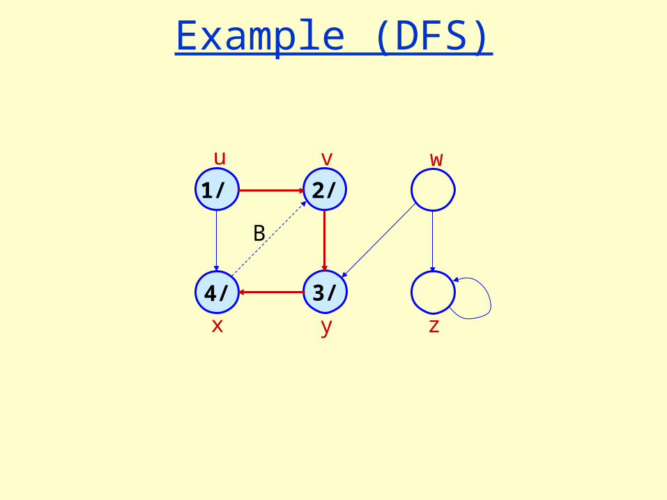
Example (DFS)

1/

4/ 3/

2/

u v w

x y z

B

Example (DFS)

1/

4/5 3/

2/

u v w

x y z

B

Example (DFS)

1/

4/5 3/6

2/

u v w

x y z

B

Example (DFS)

1/

4/5 3/6

2/7

u v w

x y z

B

Example (DFS)

1/

4/5 3/6

2/7

u v w

x y z

BF

Example (DFS)

1/8

4/5 3/6

2/7

u v w

x y z

BF

Example (DFS)

1/8

4/5 3/6

2/7 9/

u v w

x y z

BF

Example (DFS)

1/8

4/5 3/6

2/7 9/

u v w

x y z

BF C

Example (DFS)

1/8

4/5 3/6 10/

2/7 9/

u v w

x y z

BF C

Example (DFS)

1/8

4/5 3/6 10/

2/7 9/

u v w

x y z

BF C

B

Example (DFS)

1/8

4/5 3/6 10/11

2/7 9/

u v w

x y z

BF C

B

Example (DFS)

1/8

4/5 3/6 10/11

2/7 9/12

u v w

x y z

BF C

B

Analysis of DFS

Loops on lines 1-2 & 5-7 take (V) time, excluding time to execute DFS-Visit.

DFS-Visit is called once for each white vertex vV when it’s painted gray the first time. Lines 3-6 of DFS-Visit is executed |Adj[v]| times. The total cost of executing DFS-Visit is vV|Adj[v]| = (E)

Total running time of DFS is (V+E).

Parenthesis TheoremTheorem 22.7

For all u, v, exactly one of the following holds:

1. d[u] < f [u] < d[v] < f [v] or d[v] < f [v] < d[u] < f [u] and neither u nor v is a descendant of the other.

2. d[u] < d[v] < f [v] < f [u] and v is a descendant of u.

3. d[v] < d[u] < f [u] < f [v] and u is a descendant of v.

Theorem 22.7

For all u, v, exactly one of the following holds:

1. d[u] < f [u] < d[v] < f [v] or d[v] < f [v] < d[u] < f [u] and neither u nor v is a descendant of the other.

2. d[u] < d[v] < f [v] < f [u] and v is a descendant of u.

3. d[v] < d[u] < f [u] < f [v] and u is a descendant of v.

So d[u] < d[v] < f [u] < f [v] cannot happen. Like parentheses:

OK: ( ) [ ] ( [ ] ) [ ( ) ] Not OK: ( [ ) ] [ ( ] )

Corollary

v is a proper descendant of u if and only if d[u] < d[v] < f [v] < f [u].

Example (Parenthesis Theorem)

3/6

4/5 7/8 12/13

2/9 1/10

y z s

x w v

B F

14/15

11/16

u

t

C C C

C B

(s (z (y (x x) y) (w w) z) s) (t (v v) (u u) t)

Depth-First Trees Predecessor subgraph defined slightly different from

that of BFS. The predecessor subgraph of DFS is G = (V, E) where

E ={([v],v) : v V and [v] NIL}.» How does it differ from that of BFS?

» The predecessor subgraph G forms a depth-first forest composed of several depth-first trees. The edges in E are called tree edges.

Definition:Forest: An acyclic graph G that may be disconnected.

Classification of Edges Tree edge: in the depth-first forest. Found by exploring

(u, v). Back edge: (u, v), where u is a descendant of v (in the

depth-first tree). Forward edge: (u, v), where v is a descendant of u, but

not a tree edge. Cross edge: any other edge. Can go between vertices in

same depth-first tree or in different depth-first trees.

Theorem:In DFS of an undirected graph, we get only tree and back edges. No forward or cross edges.

Theorem:In DFS of an undirected graph, we get only tree and back edges. No forward or cross edges.

The DFS algorithm can be modified to classify edges as it encounters them. The key idea is that each edge (u, v) can be classified by the color of the vertex v that is reached when the edge is first explored (except that forward and cross edges are not distinguished):

1. WHITE indicates a tree edge, 2. GRAY indicates a back edge, and 3. BLACK indicates a forward or cross edge.

22.4 Topological sort A topological sort of a dag (directed acyclic

graphs) G = (V, E) is a linear ordering of all its vertices such that if G contains an edge (u, v), then u appears before v in the ordering.

TOPOLOGICAL-SORT(G)1 call DFS(G) to compute finishing times f[v] for each vertex v 2 as each vertex is finished, insert it onto the front of a linked list 3 return the linked list of vertices

Lemma 22.11 A directed graph G is acyclic if and only if a

depth-first search of G yields no back edges. Theorem 22.12 TOPOLOGICAL-SORT(G) produces a

topological sort of a directed acyclic graph G.

22.5 Strongly connected components We now consider a classic application of depth-

first search: decomposing a directed graph into its strongly connected components.

Recall that a strongly connected component of a directed graph G = (V, E) is a maximal set of vertices U V such that for every pair of vertices u and v in U, we have both that is, vertices u and v are reachable from each other.

Our algorithm for finding strongly connected components of a graph G = (V, E) uses the transpose of G, which is defined to be the graph GT = (V, ET), where ET = {(u, v): (v, u)∈E}. That is, ET consists of the edges of G with their directions reversed. Given an adjacency-list representation of G, the time to create GT is O(V + E).

TRANSPOSE-GRAPH(G)1 for each u∈G(V)2 do TG’s Adj[u]←NIL3 for each u∈G(V)4 do for each v∈G’s Adj[u]5 do insert u into TG’s Adj[v]6 G←TG

STRONGLY-CONNECTED-COMPONENTS(G) 1 call DFS(G) to compute finishing times f[u] for

each vertex u

2 compute GT

3 call DFS(GT), but in the main loop of DFS, consider the vertices in order of decreasing f[u] (as computed in line 1)

4 output the vertices of each tree in the depth-first forest of step 3 as a separate strongly connected component