elements of mathematical oncology -...
TRANSCRIPT
Elements of Mathematical Oncology
Franco Flandoli, University of Pisa
Padova 2015, Lecture 1
Franco Flandoli, University of Pisa () Elements of Mathematical Oncology Padova 2015, Lecture 1 1 / 30
Structure of the course
1 Part I: Macroscopic models (lectures 1, 2, 3)
2 Part II: Microscopic models (lectures 4, 5, 6)
Franco Flandoli, University of Pisa () Elements of Mathematical Oncology Padova 2015, Lecture 1 2 / 30
Structure of the course: Part I
1 Introduction: an example of reaction diffusion system
2 FKPP model
3 Back to more complex models
Franco Flandoli, University of Pisa () Elements of Mathematical Oncology Padova 2015, Lecture 1 3 / 30
Structure of the course: Part II
4 Introduction to interacting systems of cells; comments on in situ case;how to model proliferation
5 Short, long and intermediate range interactions and their macroscopiclimits (heuristics)
6 Rigorous details on mean field (long range) and intermediate rangeproblems.
Franco Flandoli, University of Pisa () Elements of Mathematical Oncology Padova 2015, Lecture 1 4 / 30
Introduction to a few elements of biology of cancer
Cancer starts from a single normal cell. It requires a sequence ofgenetic modifications.
Main new feature of a cancer cell: uncontrolled duplication
Tumor mass starts to be detectable when there are around 109 cancercells.
Franco Flandoli, University of Pisa () Elements of Mathematical Oncology Padova 2015, Lecture 1 5 / 30
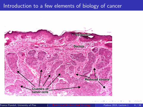
Introduction to a few elements of biology of cancer
Franco Flandoli, University of Pisa () Elements of Mathematical Oncology Padova 2015, Lecture 1 6 / 30
Introduction to a few elements of biology of cancer
A tumor can be in different phases.
The initial phase is called in situ.
Growth without free diffusion.
Then there is the invasive phase, with diffusion.
We shall see also the angiogenic cascade (or phase).
Franco Flandoli, University of Pisa () Elements of Mathematical Oncology Padova 2015, Lecture 1 7 / 30
Macroscopic and microscopic models
Cancer is a phenomenon at cell level, a few micron
which become visible and dangerous at the scale of a few millimetersor centimeters, the tissue level.
These two levels, cell and tissue ones, will be called microscopic andmacroscopic levels.
Stochastic particle systems to describe cell motion and interaction(microscopic)
Deterministic partial differential equations to describe a tumor fromthe macroscopic viewpoint.
Link between the two levels: macroscopic limit.
Franco Flandoli, University of Pisa () Elements of Mathematical Oncology Padova 2015, Lecture 1 8 / 30
An advanced model of invasive tumor with angiogenesis
Lectures 1 and 3 are devoted to a reaction-diffusion model for invasive +angiogenetic phases.It is taken from:
P. Hinow, P. Gerlee, L. J. McCawley, V. Quaranta, M. Ciobanu, S.Wang, J. M. Graham, B. P. Ayati, J. Claridge, K. R. Swanson, M.Loveless, A. R. A. Anderson, A spatial model of tumor-hostinteraction: application of chemoterapy, Math. Biosc. Engin. 2009.
It is just one of the very many models, devoted to different phases,different phenomena etc.It is a system of 7 equations (PDEs and ODEs), for 7 quantities.
Franco Flandoli, University of Pisa () Elements of Mathematical Oncology Padova 2015, Lecture 1 9 / 30
Normoxic, hypoxic and apoptotic cells
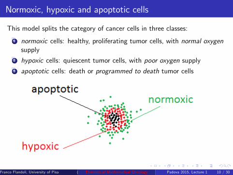
This model splits the category of cancer cells in three classes:
1 normoxic cells: healthy, proliferating tumor cells, with normal oxygensupply
2 hypoxic cells: quiescent tumor cells, with poor oxygen supply3 apoptotic cells: death or programmed to death tumor cells
Franco Flandoli, University of Pisa () Elements of Mathematical Oncology Padova 2015, Lecture 1 10 / 30
PDE for normoxic cells
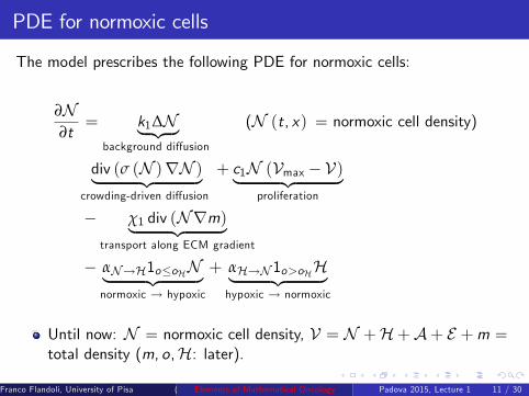
The model prescribes the following PDE for normoxic cells:
∂N∂t
= k1∆N︸ ︷︷ ︸background diffusion
(N (t, x) = normoxic cell density)
div (σ (N )∇N )︸ ︷︷ ︸crowding-driven diffusion
+ c1N (Vmax − V)︸ ︷︷ ︸proliferation
− χ1 div (N∇m)︸ ︷︷ ︸transport along ECM gradient
− αN→H1o≤oHN︸ ︷︷ ︸normoxic → hypoxic
+ αH→N 1o>oHH︸ ︷︷ ︸hypoxic → normoxic
Until now: N = normoxic cell density, V = N +H+A+ E +m =total density (m, o,H: later).
Franco Flandoli, University of Pisa () Elements of Mathematical Oncology Padova 2015, Lecture 1 11 / 30
ODE for hypoxic cells
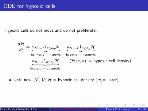
Hypoxic cells do not move and do not proliferate:
dHdt
= αN→H1o≤oHN︸ ︷︷ ︸normoxic → hypoxic
− αH→N 1o≥oHH︸ ︷︷ ︸hypoxic → normoxic
− αH→A1o≤oAH︸ ︷︷ ︸hypoxic → apoptotic
(H (t, x) = hypoxic cell density)
Until now: N , V ; H = hypoxic cell density (m, o: later).
Franco Flandoli, University of Pisa () Elements of Mathematical Oncology Padova 2015, Lecture 1 12 / 30
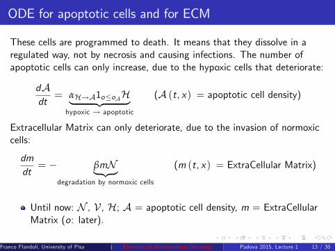
ODE for apoptotic cells and for ECM
These cells are programmed to death. It means that they dissolve in aregulated way, not by necrosis and causing infections. The number ofapoptotic cells can only increase, due to the hypoxic cells that deteriorate:
dAdt
= αH→A1o≤oAH︸ ︷︷ ︸hypoxic → apoptotic
(A (t, x) = apoptotic cell density)
Extracellular Matrix can only deteriorate, due to the invasion of normoxiccells:
dmdt= − βmN︸ ︷︷ ︸
degradation by normoxic cells
(m (t, x) = ExtraCellular Matrix)
Until now: N , V , H; A = apoptotic cell density, m = ExtraCellularMatrix (o: later).
Franco Flandoli, University of Pisa () Elements of Mathematical Oncology Padova 2015, Lecture 1 13 / 30
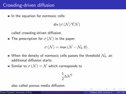
Crowding-driven diffusion
In the equation for normoxic cells:
div (σ (N )∇N )
called crowding-driven diffusion.
The prescription for σ (N ) in the paper:
σ (N ) = max (N −N0, 0) .
When the density of normoxic cells passes the threshold N0, anadditional diffusion starts.
Similar to σ (N ) = N which corresponds to
12
∆N 2
also called porous media diffusion.
Franco Flandoli, University of Pisa () Elements of Mathematical Oncology Padova 2015, Lecture 1 14 / 30
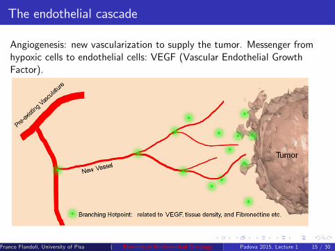
The endothelial cascade
Angiogenesis: new vascularization to supply the tumor. Messenger fromhypoxic cells to endothelial cells: VEGF (Vascular Endothelial GrowthFactor).
Franco Flandoli, University of Pisa () Elements of Mathematical Oncology Padova 2015, Lecture 1 15 / 30
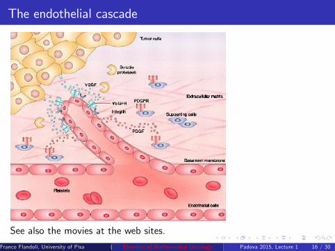
The endothelial cascade
See also the movies at the web sites.
Franco Flandoli, University of Pisa () Elements of Mathematical Oncology Padova 2015, Lecture 1 16 / 30
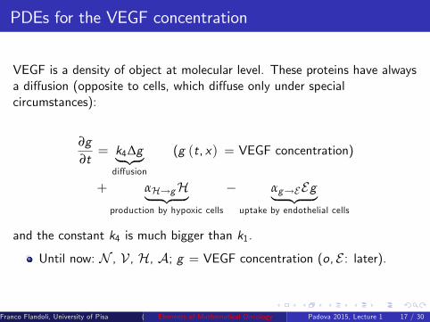
PDEs for the VEGF concentration
VEGF is a density of object at molecular level. These proteins have alwaysa diffusion (opposite to cells, which diffuse only under specialcircumstances):
∂g∂t= k4∆g︸ ︷︷ ︸
diffusion
(g (t, x) = VEGF concentration)
+ αH→gH︸ ︷︷ ︸production by hypoxic cells
− αg→EEg︸ ︷︷ ︸uptake by endothelial cells
and the constant k4 is much bigger than k1.
Until now: N , V , H, A; g = VEGF concentration (o, E : later).
Franco Flandoli, University of Pisa () Elements of Mathematical Oncology Padova 2015, Lecture 1 17 / 30
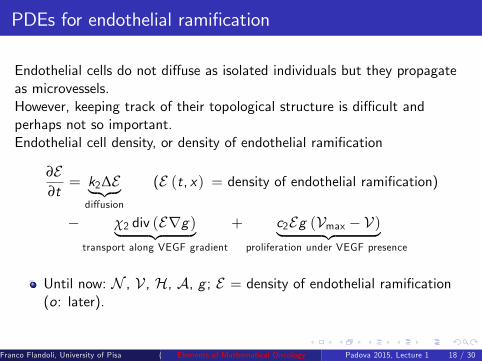
PDEs for endothelial ramification
Endothelial cells do not diffuse as isolated individuals but they propagateas microvessels.However, keeping track of their topological structure is diffi cult andperhaps not so important.Endothelial cell density, or density of endothelial ramification
∂E∂t= k2∆E︸ ︷︷ ︸
diffusion
(E (t, x) = density of endothelial ramification)
− χ2 div (E∇g)︸ ︷︷ ︸transport along VEGF gradient
+ c2Eg (Vmax − V)︸ ︷︷ ︸proliferation under VEGF presence
Until now: N , V , H, A, g ; E = density of endothelial ramification(o: later).
Franco Flandoli, University of Pisa () Elements of Mathematical Oncology Padova 2015, Lecture 1 18 / 30

PDEs for oxygen concentration
Oxygen is also molecular-level hence it diffuses, with k3 is much biggerthan k1
∂o∂t= k3∆o︸ ︷︷ ︸
diffusion
(o (t, x) = oxygen concentration)
+ c3E (omax − o)︸ ︷︷ ︸production by endothelial cells
− αo→N ,H,E (N +H+ E) o︸ ︷︷ ︸uptake by all living cells
− γo︸︷︷︸oxygen decay
The system for N , V , H, A, g , E , o is complete.
Franco Flandoli, University of Pisa () Elements of Mathematical Oncology Padova 2015, Lecture 1 19 / 30
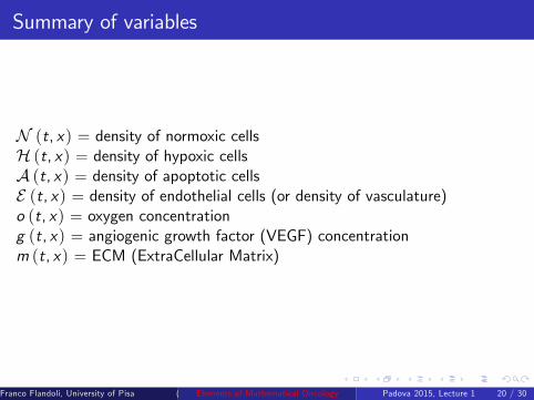
Summary of variables
N (t, x) = density of normoxic cellsH (t, x) = density of hypoxic cellsA (t, x) = density of apoptotic cellsE (t, x) = density of endothelial cells (or density of vasculature)o (t, x) = oxygen concentrationg (t, x) = angiogenic growth factor (VEGF) concentrationm (t, x) = ECM (ExtraCellular Matrix)
Franco Flandoli, University of Pisa () Elements of Mathematical Oncology Padova 2015, Lecture 1 20 / 30
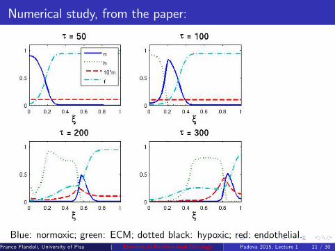
Numerical study, from the paper:
Blue: normoxic; green: ECM; dotted black: hypoxic; red: endothelial.Franco Flandoli, University of Pisa () Elements of Mathematical Oncology Padova 2015, Lecture 1 21 / 30
Stochastic dynamics associated to some element of theprevious model
The next last slides of Lecture 1 have the purpose to show the easiestmathematical elements of a microscopic, cell-level, description of theprevious PDE system.
Some elements of the previous model have a straightforwardtranslation into a microscopic, cell level, random dynamics.
Franco Flandoli, University of Pisa () Elements of Mathematical Oncology Padova 2015, Lecture 1 22 / 30
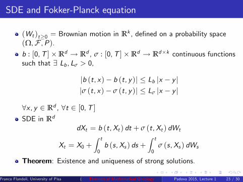
SDE and Fokker-Planck equation
(Wt )t≥0 = Brownian motion in Rk , defined on a probability space(Ω,F ,P).b : [0,T ]×Rd → Rd , σ : [0,T ]×Rd → Rd×k continuous functionssuch that ∃ Lb , Lσ > 0,
|b (t, x)− b (t, y)| ≤ Lb |x − y ||σ (t, x)− σ (t, y)| ≤ Lσ |x − y |
∀x , y ∈ Rd , ∀t ∈ [0,T ]SDE in Rd
dXt = b (t,Xt ) dt + σ (t,Xt ) dWt
Xt = X0 +∫ t
0b (s,Xs ) ds +
∫ t
0σ (s,Xs ) dWs
Theorem: Existence and uniqueness of strong solutions.
Franco Flandoli, University of Pisa () Elements of Mathematical Oncology Padova 2015, Lecture 1 23 / 30
SDE and Fokker-Planck equation
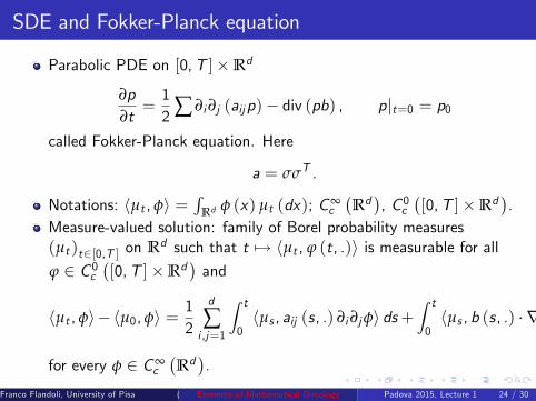
Parabolic PDE on [0,T ]×Rd
∂p∂t=12 ∑ ∂i∂j (aijp)− div (pb) , p|t=0 = p0
called Fokker-Planck equation. Here
a = σσT .
Notations: 〈µt , φ〉 =∫
Rd φ (x) µt (dx); C∞c
(Rd), C 0c
([0,T ]×Rd
).
Measure-valued solution: family of Borel probability measures(µt )t∈[0,T ] on Rd such that t 7→ 〈µt , ϕ (t, .)〉 is measurable for allϕ ∈ C 0c
([0,T ]×Rd
)and
〈µt , φ〉− 〈µ0, φ〉 =12
d
∑i ,j=1
∫ t
0〈µs , aij (s, .) ∂i∂jφ〉 ds+
∫ t
0〈µs , b (s, .) · ∇φ〉 ds
for every φ ∈ C∞c
(Rd).
Franco Flandoli, University of Pisa () Elements of Mathematical Oncology Padova 2015, Lecture 1 24 / 30
SDE and Fokker-Planck equation
TheoremThe law µt of Xt is a measure-valued solution of the the Fokker-Planckequation.
Under suitable assumptions of non-degeneracy of aij , if µ0 has a density p0then also µt has a density p (t, ·), often with some regularity gained by theparabolic structures.
Franco Flandoli, University of Pisa () Elements of Mathematical Oncology Padova 2015, Lecture 1 25 / 30
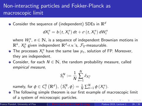
Non-interacting particles and Fokker-Planck asmacroscopic limit
Consider the sequence of (independent) SDEs in Rd
dX nt = b (t,Xnt ) dt + σ (t,X nt ) dW
nt
where W nt , n ∈N, is a sequence of independent Brownian motions in
Rk , X n0 given independent Rd -r.v.’s, F0-measurable.The processes X nt have the same law µt , solution of FP. Moreover,they are independent.Consider, for each N ∈N, the random probability measure, calledempirical measure,
SNt :=1N
N
∑n=1
δX nt
namely, for φ ∈ C 0c(Rd),⟨SNt , φ
⟩= 1
N ∑Nn=1 φ (X nt ).
The following simple theorem is our first example of macroscopic limitof a system of microscopic particles.
Franco Flandoli, University of Pisa () Elements of Mathematical Oncology Padova 2015, Lecture 1 26 / 30

Non-interacting particles and Fokker-Planck asmacroscopic limit
Theorem
For every t ∈ [0,T ] and φ ∈ C 0c(Rd), a.s.
limN→∞
⟨SNt , φ
⟩= 〈µt , φ〉 .
In other words, SNt converges weakly, a.s., to a measure-valued solution ofthe Fokker-Planck equation.
Proof.Since φ (X nt ) are bounded i.i.d., by the strong LLN we have, a.s.,
limN→∞
⟨SNt , φ
⟩= E
[φ(X 1t)]= 〈µt , φ〉 .
A.s. convergence is uniform in φ, by a countable density argument.
Franco Flandoli, University of Pisa () Elements of Mathematical Oncology Padova 2015, Lecture 1 27 / 30
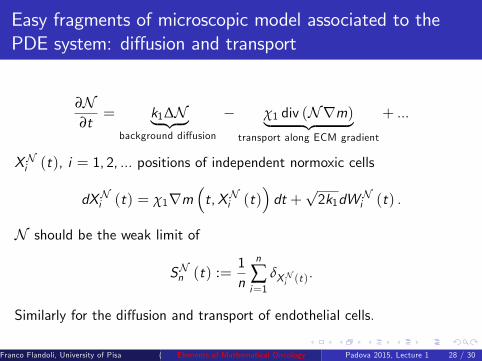
Easy fragments of microscopic model associated to thePDE system: diffusion and transport
∂N∂t
= k1∆N︸ ︷︷ ︸background diffusion
− χ1 div (N∇m)︸ ︷︷ ︸transport along ECM gradient
+ ...
XNi (t), i = 1, 2, ... positions of independent normoxic cells
dXNi (t) = χ1∇m(t,XNi (t)
)dt +
√2k1dWNi (t) .
N should be the weak limit of
SNn (t) :=1n
n
∑i=1
δXNi (t).
Similarly for the diffusion and transport of endothelial cells.
Franco Flandoli, University of Pisa () Elements of Mathematical Oncology Padova 2015, Lecture 1 28 / 30
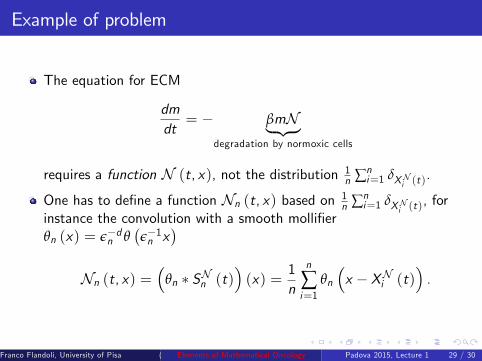
Example of problem
The equation for ECM
dmdt= − βmN︸ ︷︷ ︸
degradation by normoxic cells
requires a function N (t, x), not the distribution 1n ∑n
i=1 δXNi (t).
One has to define a function Nn (t, x) based on 1n ∑n
i=1 δXNi (t), for
instance the convolution with a smooth mollifierθn (x) = ε−dn θ
(ε−1n x
)Nn (t, x) =
(θn ∗ SNn (t)
)(x) =
1n
n
∑i=1
θn(x − XNi (t)
).
Franco Flandoli, University of Pisa () Elements of Mathematical Oncology Padova 2015, Lecture 1 29 / 30
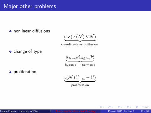
Major other problems
nonlinear diffusionsdiv (σ (N )∇N )︸ ︷︷ ︸
crowding-driven diffusion
change of typeαH→N 1o≥oHH︸ ︷︷ ︸hypoxic → normoxic
proliferationc1N (Vmax − V)︸ ︷︷ ︸
proliferation
Franco Flandoli, University of Pisa () Elements of Mathematical Oncology Padova 2015, Lecture 1 30 / 30