eleventh floor menzies building clayton vic 3168 australia ... · e5.3 graphical solution to the...
TRANSCRIPT

CENTRE of
POLICYSTUDIES and
the IMPACTPROJECT
Eleventh FloorMenzies BuildingMonash University Wellington RoadCLAYTON Vic 3168 AUSTRALIATelephone: from overseas:(03) 905 2398, (03) 905 5112 61 3 905 2398 or
61 3 905 5112Fax numbers: from overseas:(03) 905 2426, (03)905 5486 61 3 905 2426 or 61 3 905 5486e-mail [email protected]
The Mathematical ProgrammingApproach to Applied General
Equilibrium Modelling:Notes and Problems
by
Peter B. DIXON
Centre of Policy Studies
Monash University
Working Paper No. I-50 April 1991
ISSN 1031 9034 ISBN 0 642 10113 2
The Centre of Policy Studies (COPS) is a research centre at Monash Universitydevoted to quantitative analysis of issues relevant to Australian economic policy.The Impact Project is a cooperative venture between the Australian FederalGovernment and Monash University, La Trobe University, and the AustralianNational University. During the three years January 1993 to December 1995 COPSand Impact will operate as a single unit at Monash University with the task ofconstructing a new economy-wide policy model to be known as MONASH. Thisinitiative is supported by the Industry Commission on behalf of the CommonwealthGovernment, and by several other sponsors. The views expressed herein do notnecessarily represent those of any sponsor or government.

ii
iii
The Mathematical Programming
Approach to Applied General
Equilibrium Modelling:
Notes and Problems
by
Peter B. DixonCentre of Policy Studies
Monash University

iv

v
Preface
The mathematical programming approachto applied general equilibrium analysis, althoughno longer the dominant tool, is still useful, fromat least two points of view:
• it neatly integrates into an economy-wideframework the microeconomic theory ofthe behaviour of agents constrained byinequalities; and
• it provides a useful approach for com-puting the solutions of some generalequilibrium problems not solvable withthe current GEMPACK software (see, e.g.,Dixon (1991), cited below on p. 16).
The material contained in this paper wasmeant to be included in our forthcominggraduate-level text (Peter B. DI X O N , B.R.PARMENTER, Alan A. POWELL and P.J. WILCOXEN,Notes and Problems in Applied GeneralEquilibrium Economics, Amsterdam, North-Holland), but space limitations led to our reluc-tant exclusion of it from the text. Publication inthe Impact series will mean that those who findthe approach in our textbook useful will be ableto apply the same method towards masteringmathematical programming in a general equi-librium context.
Peter B. DixonApril 1991

vi
ContentsPreface v
1 Introduction 1
2 Normative versus Positive Analysis 10
3 Goals, Reading Guide and References 11Reading guide 12References 16
Exercise 1 The implications of technical change in a wine-cloth economy 18
Section 1 What can be produced? 18
Section 2 What will be produced? 21
Section 3 Commodity prices and real wages 21Section 4 The effects of a change in production techniques 22
ANSWER TO EXERCISE 1 30
Exercise 2 A single-consumer linear economy 32ANSWER TO EXERCISE 2 33
Exercise 3 The utility possibilities frontier 36ANSWER TO EXERCISE 3 37
Exercise 4 A multiple-consumer linear economy 42ANSWER TO EXERCISE 4 44
Exercise 5 A linear economy with a utilitymaximizing consumer 46
ANSWER TO EXERCISE 5 49
Exercise 6 A linear economy with several utilitymaximizing consumers 58
ANSWER TO EXERCISE 6 61
Exercise 7 An introduction to the specialization prob-lem in models of small open economies 66
ANSWER TO EXERCISE 7 69
Exercise 8 Tariffs, export subsidies and transport costsin a linear model of a small open economy 74
ANSWER TO EXERCISE 8 77
Exercise 9 A long-run planning model with investment: the snapshot approach 94
ANSWER TO EXERCISE 9 97
APPENDIXBackground Notes on the Theory of Linear Programming
A1 The standard linear programming problem 105
A2 Necessary and sufficient conditions for thesolution of the standard linear program-ming problem 105
A3 Basic solutions 106
A4 Proposition on the existence of basicsolutions 106
vii
List of Tables
E1.1 Current Production Techniques: Input-OutputCoefficients 18
E1.2 Production Techniques after an Improvement inthe Technique for Producing Cloth 20
E1.3 The Wine-Cloth Economy before and after theImprovement in the Technique for Producing Cloth 23
E1.4 Occupational Shares in the Workforce 27
E8.1 Model Solutions under Various Rates ofTariff and Export Subsidy 85
List of Figures
1.1 Utility possibilities set 6
E1.1 Net annual production possibilities 19
E1.2 Net annual production possibilities under theinitial production techniques 25
E1.3 Net annual production possibilities after the im-provement in the technique for producing cloth 25
E3.1 Utility possibilities frontiers 40
E5.1 Indifference curves for a consumer having utilityfunction (E5.6) — (E5.7) 51
E5.2 Indifference map and budget line for the consumerin model (E5.1) — (E5.4), assuming (E5.8) — (E5.10) 53
E5.3 Graphical solution to the problem on the right handside of (E5.36) 57
E5.4 Indifference map and budget line for the consumerin model (E5.1) — (E5.4), assuming (E5.8) and(E5.10) — (E5.12) 59
E8.1 Cycling in an iterative process 90
E8.2 Exchange rate solution in a special case of the
model (E8.1) — (E8.11) 93

1
The Mathematical Programming Approach to Applied General
Equilibrium Modelling: Notes and Problems
by
Peter B. Dixon
Centre of Policy Studies, Monash University
1 Introduction
General equilibrium models can often be formulated asmathematical programming (i.e., constrained optimization) problems.To illustrate this approach, we consider a 2-consumer, 2-good, puretrade (no production) model in which the initial endowments are
Z1 =
100
0 , Z2 =
0
100 , (1.1)
i.e., consumer 1 owns 100 units of good 1 and consumer 2 owns 100units of good 2. We assume that consumer 1's preferences aredescribed by the utility function
U1(C1) = ln(C11) + ln(C12) (1.2)
where C11 and C12 are his consumption levels for goods 1 and 2 and C1is the vector (C11, C12) ′. Similarly, we assume that consumer 2's utilityfunction is
U2(C2) = ln(C21) + ln(C22) . (1.3)
The problem of solving this model is to find non-negative valuesfor the product prices (denoted by the vector P' ≡ (P1 , P2 )), theconsumption vectors (C1 and C2) and the consumer incomes (Y1 and Y2)which jointly satisfy the conditions:
Ci maximizes Ui(Ci) subject to P′Ci ≤ Yi , i=1,2 , ( i )
Σi=1
2
Ci – Σi=1
2
Zi ≤ 0 , (ii)1
1 Notice that the right hand side of condition (ii) is a 2 ×1 vector of zeros. Theright hand side of (iii) is a scalar. Although we use the same symbol, namely0, the distinction is clear from the context.

2 Peter B. Dixon
P′
Σ
i=1
2
Ci– Σi=1
2
Z i = 0 , (iii)
and
P′Zi = Yi , i=1,2 . (iv)
Condition (i) says that consumers maximize their utilities subject totheir budget constraints. Condition (ii) says that demand for each goodis less than or equal to supply. This condition combined with (iii)implies that goods in excess supply have zero price. Condition (iv) saysthat consumers’ incomes are the values of their initial endowments. Aprice normalization condition must be added if we want to tie down theabsolute values for P1 and P2. We also know from Walras' law that eitherthe market clearing condition for one of the goods or the definition ofincome for one of the consumers could be eliminated. For the present,however, we will leave the model in the form (i) – (iv).
Perhaps the most obvious approach to solving generalequilibrium models is via excess demand functions. Applying thisapproach to the model (i) - (iv), we first derive the consumer demandequations from condition (i). Under (1.2) and (1.3) we obtain2
Cij = 12
YiPj
, i, j=1,2 . (1.4)
Next we use (iv) to eliminate the Yi's, i.e., we write (1.4) as
Cij = 12
P′ZiPj
, i,j=1,2 . (1.5)
With the Zis given by (1.1), (1.5) reduces to
C 1j=50P 1/ Pj,j=1 ,2,
C2j=50P 2/Pj ,j=1,2.(1.6)
2 If Pj were zero, then under (1.2) and (1.3), demand for good j would beunlimited. Because supply is finite, we may assume (in view of condition(ii)) that neither price is zero.
The Mathematical Programming Approach to Applied General Equilibrium 3
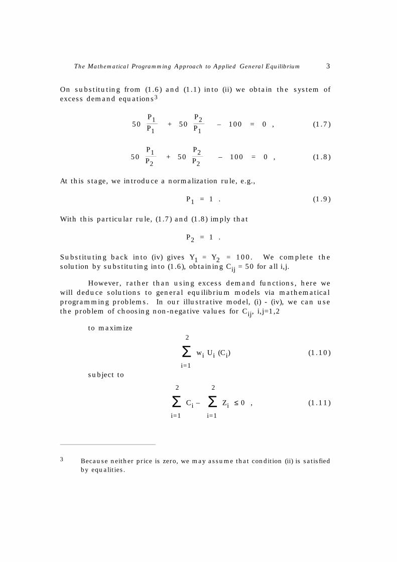
On substituting from (1.6) and (1.1) into (ii) we obtain the system ofexcess demand equations3
50 P1P1
+ 50 P2P1
– 100 = 0 , (1.7)
50 P1P2
+ 50 P2P2
– 100 = 0 , (1.8)
At this stage, we introduce a normalization rule, e.g.,
P1 = 1 . (1.9)
With this particular rule, (1.7) and (1.8) imply that
P2 = 1 .
Substituting back into (iv) gives Y1 = Y2 = 100. We complete thesolution by substituting into (1.6), obtaining Cij = 50 for all i,j.
However, rather than using excess demand functions, here wewill deduce solutions to general equilibrium models via mathematicalprogramming problems. In our illustrative model, (i) - (iv), we can usethe problem of choosing non-negative values for Cij, i,j=1,2
to maximize
Σi=1
2
wi Ui (Ci) (1.10)
subject to
Σi=1
2
Ci – Σi=1
2
Zi ≤ 0 , (1.11)
3 Because neither price is zero, we may assume that condition (ii) is satisfiedby equalities.

4 Peter B. Dixon
where the wis are weights satisfying
Σi=1
2
wi = 1 . (1.12)
In problem (1.10) – (1.11), we allocate the available
commodities to maximize a weighted average of the utilities of the two
consumers. We try to set the weights so that the consumption vectors
allocated to the consumers are consistent with their budget constraints.
In the present example where (1.1), (1.2) and (1.3) apply, it is
intuitively clear that we should set w1 = w2 = 12. Then (1.10) – (1.11)
can be written as:
choose Cij , i,j=1,2
to maximize
12
{ }ln(C11) + ln(C12) + 12
{ }ln(C21) + ln(C22) (1.13)
subject to
Σi=1
2
Cij = 100 , j=1,2 . (1.14)4
To solve (1.13) – (1.14) we note the if C_
ij, i,j=1,2, is a solution, then
there exist P_
1, P_
2 ≥ 0 such that
1/(2C_
ij) = P_
j , i=1,2, j=1,2 (1.15)
and
4 We have written the constraints as equalities. The maximization of (1.13)requires that all of the available supplies be used.
The Mathematical Programming Approach to Applied General Equilibrium 5
Σi=1
2
C_
ij = 100 , j=1,2 . (1.16)
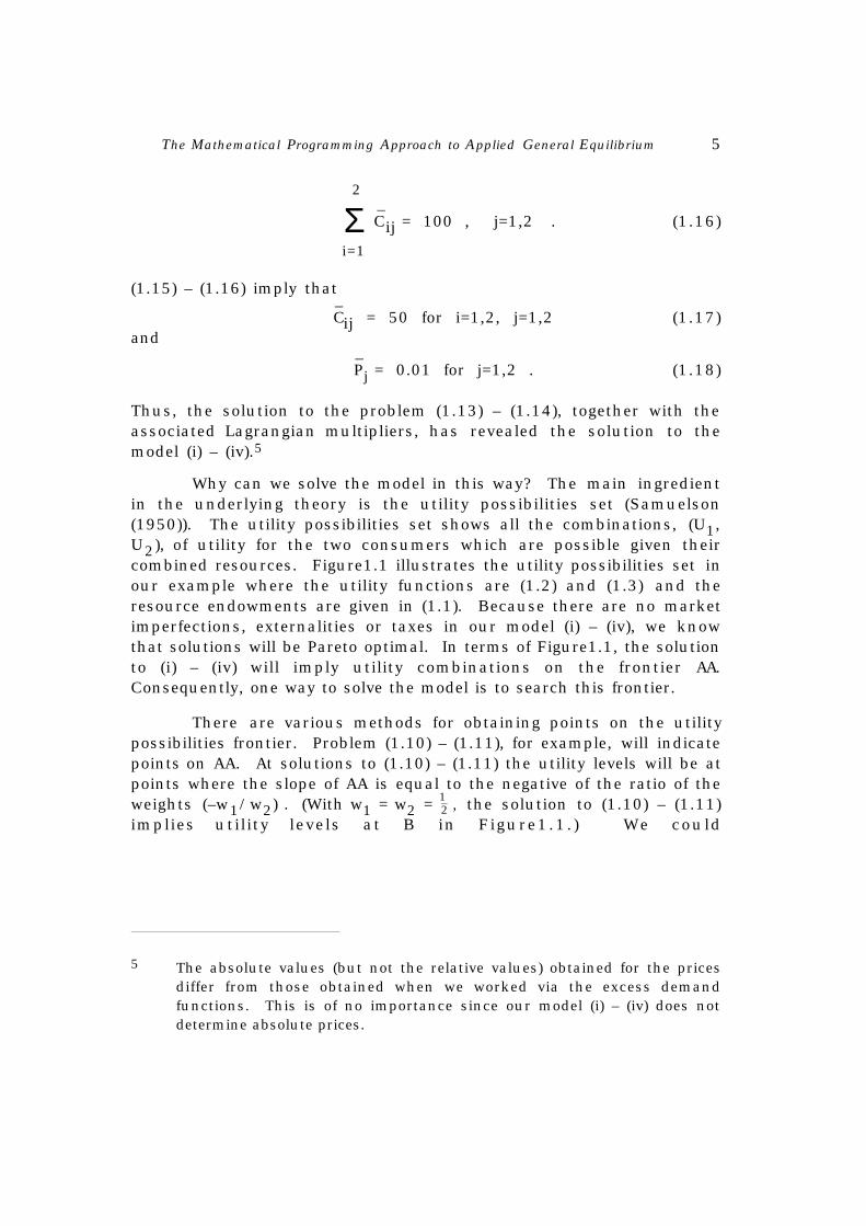
(1.15) – (1.16) imply that
C_
ij = 50 for i=1,2, j=1,2 (1.17)and
P_
j = 0.01 for j=1,2 . (1.18)
Thus, the solution to the problem (1.13) – (1.14), together with theassociated Lagrangian multipliers, has revealed the solution to themodel (i) – (iv).5
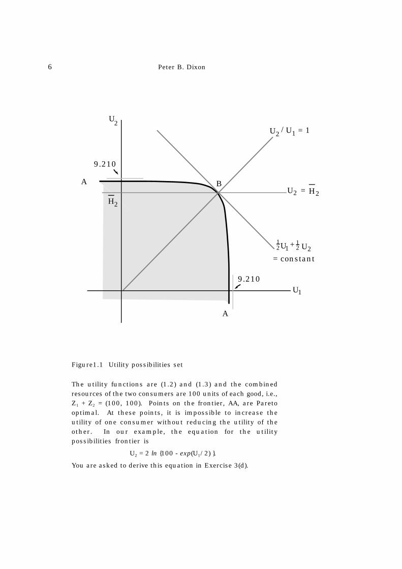
Why can we solve the model in this way? The main ingredientin the underlying theory is the utility possibilities set (Samuelson(1950)). The utility possibilities set shows all the combinations, (U1,U2), of utility for the two consumers which are possible given theircombined resources. Figure1.1 illustrates the utility possibilities set inour example where the utility functions are (1.2) and (1.3) and theresource endowments are given in (1.1). Because there are no marketimperfections, externalities or taxes in our model (i) – (iv), we knowthat solutions will be Pareto optimal. In terms of Figure1.1, the solutionto (i) – (iv) will imply utility combinations on the frontier AA.Consequently, one way to solve the model is to search this frontier.
There are various methods for obtaining points on the utilitypossibilities frontier. Problem (1.10) – (1.11), for example, will indicatepoints on AA. At solutions to (1.10) – (1.11) the utility levels will be atpoints where the slope of AA is equal to the negative of the ratio of theweights (–w1/w2) . (With w1 = w2 = 12 , the solution to (1.10) – (1.11)implies utility levels at B in Figure1.1.) We could
5 The absolute values (but not the relative values) obtained for the pricesdiffer from those obtained when we worked via the excess demandfunctions. This is of no importance since our model (i) – (iv) does notdetermine absolute prices.
6 Peter B. Dixon
9.210
9.210
U2
A
H2
B
U2/U1 = 1
U 2= H2
12 U+U 2
12
= constant1
U1
A
Figure1.1 Utility possibilities set
The utility functions are (1.2) and (1.3) and the combinedresources of the two consumers are 100 units of each good, i.e.,Z1 + Z2 = (100, 100). Points on the frontier, AA, are Paretooptimal. At these points, it is impossible to increase theutility of one consumer without reducing the utility of theother. In our example, the equation for the utilitypossibilities frontier is
U2 = 2 ln {100 - exp(U1/2) }.
You are asked to derive this equation in Exercise 3(d).

The Mathematical Programming Approach to Applied General Equilibrium 7
also generate points on AA by solving problems of the form: choose non-negative values for Cij, i,j=1,2
to maximizeU1(C11, C12) (1.19)
subject to
Σi=1
2
Cij – Σi=1
2
Zij ≤ 0 , j=1,2 (1.20)
and
U2(C21, C22) >_ H2 . (1.21)
In this problem, we allocate the available commodities so as to maximizeconsumer 1's utility subject to consumer 2 achieving a utility level of atleast H2. (If H2 were set at H
_2 in our example, then problem (1.19) –
(1.21) would generate point B in Figure1.1).
A third approach to generating points on AA is to solve problemsof the form: choose non-negative values for Cij, i,j=1,2
to maximizeU1(C11, C12) (1.22)
subject to
Σi=1
2
Cij – Σi=1
2
Zij ≤ 0 , j=1,2 (1.23)
and
U2(C21, C22) >_ β U1(C11, C12) . (1.24)
This time, we maximize consumer 1's utility subject to consumer 2achieving a utility level of at least β times that of consumer 1. (If β wereset at 1 in our example, then problem (1.22) – (1.24) would generatepoint B in Figure1.1.)
The question remains of how we should set the wis in (1.10) –(1.11) or the H2 in (1.19) – (1.21) or the β in (1.22) – (1.24) so that theparticular point generated on the utility possibilities frontier indicates asolution to our model (i) – (iv). How could we have proceeded withproblem (1.10) – (1.11), for example, if we had not known the
8 Peter B. Dixon
appropriate values (w1 = 12, w2 = 12) for the weights a priori? Except invery simple cases, we must adopt an iterative approach. That is, wemust make an initial guess of the appropriate values for the wis; solveproblem (1.10) – (1.11); use information from our solution to improveour guess of the wis; re-solve (1.10) – (1.11); improve our guess, etc. Ifin our numerical example, we had made as an initial guess for theweights
w(1)1 =
14 , w
(1)2 =
34 , (1.25)6
then our initial solution to problem (1.10) – (1.11) would have been
(C_(1)
1 )′ = (25, 25) , (C
_(1)2 )′
= (75, 75) , (1.26)7
with the Lagrangian multipliers being
( P_(1))′
= (0.01, 0.01) . (1.27)
Interpreting the Lagrangian multipliers as commodity prices, this wouldhave implied a value of
( P_(1))′(C
_(1)1 ) = 0.5
for consumer 1's expenditure and
( P_(1))′
Z1 = 1.0
for the consumer's income. For consumer 2, expenditure and incomewould have been 1.5 and 1.0 respectively. These expenditure andincome levels are inconsistent with condition (i). To move towards asolution to model (i) – (iv), we would have had to increase w1 relative tow2 and to re-solve problem (1.10) – (1.11). With a higher value forw1/w2, problem (1.10) – (1.11) would allocate more consumption to
6 We use the superscript (s) to denote values of variables in the sth iteration.
For example, w(1)1 and w
(1)2 are the weights in the first iteration.
7 (1.26) and (1.27) are easily established by revising (1.15) to read
1/(4C
_
1j)=P_
j,j=1,2
3/(4C_
2j)=P_j,j=1,2.
(1.28)

The Mathematical Programming Approach to Applied General Equilibrium 9
consumer 1 and less to consumer 2. Your exercises and readings willindicate various rules for moving the ws, Hs or βs which have provedeffective in practical applications.
The final question for this section is: what are the advantages ofmathematical programming as a means of solving general equilibriummodels compared with working with systems of excess demandfunctions. Proponents of the mathematical programming approachnormally emphasize dimensionality. When we work with the excessdemand functions we have n – 1 unknowns where n is the number ofcommodity prices. (One price can be eliminated via normalization.) Inprogramming problems such as (1.10) – (1.11), (1.19) – (1.21) and(1.22) – (1.24) we have to find values for k – 1 iterative variables wherek is the number of consumers. (In problem (1.10) – (1.11), one of thews can be eliminated via, for example, the normalization rule (1.12).) Inmany applied models, k (the number of consumers) is small comparedto n (the number of commodities). For instance, it is quite common totreat the household sector as if it were composed of a single utility-maximizing consumer. With k = 1, we can solve models such as (i) – (iv)simply as mathematical programming problems without any iterativesearch being required. With k = 2, our iterative search involves no morethan moving around a one-dimensional frontier such as AA in Figure1.1.Even with larger values of k, say k = 10, it may be easier to search in a(k – 1)-dimensional weight-space (or H-space or β-space) than to deriveand solve a system of excess demand functions involving, perhaps,several hundred unknown commodity prices. Of course, in choosingbetween competing computational approaches, researchers considermany factors apart from dimensionality. For example, are theprogramming problems which must be solved at each step of theweight-iteration procedure of a computationally simple form? Can theybe adequately approximated as linear programming problems? If so, hasthe local computer centre access to a cheap, user-friendly, linearprogramming package? If excess demand equations are used, is itnecessary that they be excess demand equations for commodities?Would it be preferable to work with excess demand equations forfactors? What packages are available for solving systems of non-linearequations? What modifications would be necessary before the availablepackages could be applied to systems of excess demand functions?
10 Peter B. Dixon
2 Normative Versus Positive Analysis
Some of the literature on mathematical programming modelsblurs the distinction between normative and positive analysis. It is inthe hope of helping you to keep the distinction clear that we providethis section.
In the previous section we showed how the simple model (i) –(iv) can be solved via mathematical programming. More generally, inthe programming approach to economic modelling it is assumed thatthe vector X of endogenous variables either should be set so as tomaximize or will maximize a function
f(X, Z) (2.1)subject to
g(X, Z) ≤ 0 (2.2)
where (2.2) is a set of constraints containing, for example, demand andsupply balances for commodities and factors, and Z is the vector ofexogenous variables. The Lagrangian multipliers (also called "shadowprices") associated with the constraints can normally be interpreted ascommodity and factor prices.
Some models expressed in the form (2.1) – (2.2) are intended tobe normative (prescriptive) while others are intended to be positive(descriptive). Because the distinction is important we emphasized, inthe previous paragraph, the words "should" (normative models) and"will" (descriptive models).
In normative models, positive weights may appear in theobjective function (2.1) on variables pertaining to economic growth andequality of income distribution. Alternatively, growth and distributiontargets may be included among the constraints. We may also find policyinstruments (e.g., taxes, tariffs and government spending) among thechoice variables (X). In descriptive models, (1.1) is usually an aggregateutility function formed (explicitly or implicitly) as a weighted sum of theutility functions of individual consumers where the weights reflectrelative spending power. Far from giving positive weight to incomeequality, the objective function in a descriptive model will emphasizethe preferences of relatively rich consumers.
The Mathematical Programming Approach to Applied General Equilibrium 11
This does not mean, however, that normative analysis isprecluded with a descriptive model. It means that analysis is separatedinto descriptive and normative stages. In the first stage, problem (2.1)– (2.2) is solved with different values for Z. The Z vector in adescriptive model will normally include policy instruments, thecomputations often being used to describe the effects of adoptingdifferent policies under the assumption that the economy operates as ifit were maximizing consumer utility subject to resource constraints. Inthe second stage, the welfare implications of the results of the firststage are evaluated outside the model. This stage will usually be quiteinformal. The analysts may merely state that he prefers policy A topolicy B because he estimates from his model that A will have the morefavourable impact on income distribution.
Here we will be concerned with descriptive modelling althoughreferences are made to some normative planning models.
3 Goals, Reading Guide and References
By the time you have completed your reading and finished theexercises, we hope that you will have
(1) a facility for expressing general equilibrium models asmathematical programming problems;
(2) a thorough understanding of how general equilibrium models canbe solved by a sequence of mathematical programming problems;
(3) a knowledge of how nonlinear mathematical programmingproblems with convex constraint sets and concave objectivefunctions can be solved as linear programming problems;
(4) an explanation of the overspecialization problem both in intuitiveeconomic terms (what diversifying phenomena are missing) and interms of the theory of linear programming; and
(5) a familiarity with how investment, restrictions on internationaltrade (tariffs and quotas) and taxes on commodities and factors arehandled in the mathematical programming framework.
The reading guide lists some material which will help you toachieve these goals. The readings are referred to in abbreviated form.Full citations are in the reference list. The list also contains otherreferences appearing in the chapter.
12 Peter B. Dixon
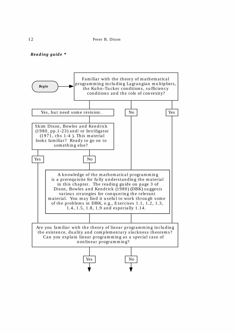
A knowledge of the mathematical programmingis a prerequisite for fully understanding the material
in this chapter. The reading guide on page 3 of Dixon, Bowles and Kendrick (1980) (DBK) suggests
various strategies for conquering the relevantmaterial. You may find it useful to work through some
of the problems in DBK, e.g., Exercises 1.1, 1.2, 1.3,1.4, 1.5, 1.8, 1.9 and especially 1.14.
Familiar with the theory of mathematicalprogramming including Lagrangian multipliers,
the Kuhn-Tucker conditions, sufficiencyconditions and the role of convexity?
Yes, but need some revision.
Skim Dixon, Bowles and Kendrick(1980, pp.1-23) and/or Intriligator
(1971, chs 1-4 ). This materiallooks familiar? Ready to go on to
something else?
No Yes
NoYes
Yes No
Are you familiar with the theory of linear programming includingthe existence, duality and complementary slackness theorems?
Can you explain linear programming as a special case ofnonlinear programming?
Reading guide *
Begin

The Mathematical Programming Approach to Applied General Equilibrium 13
NoYes
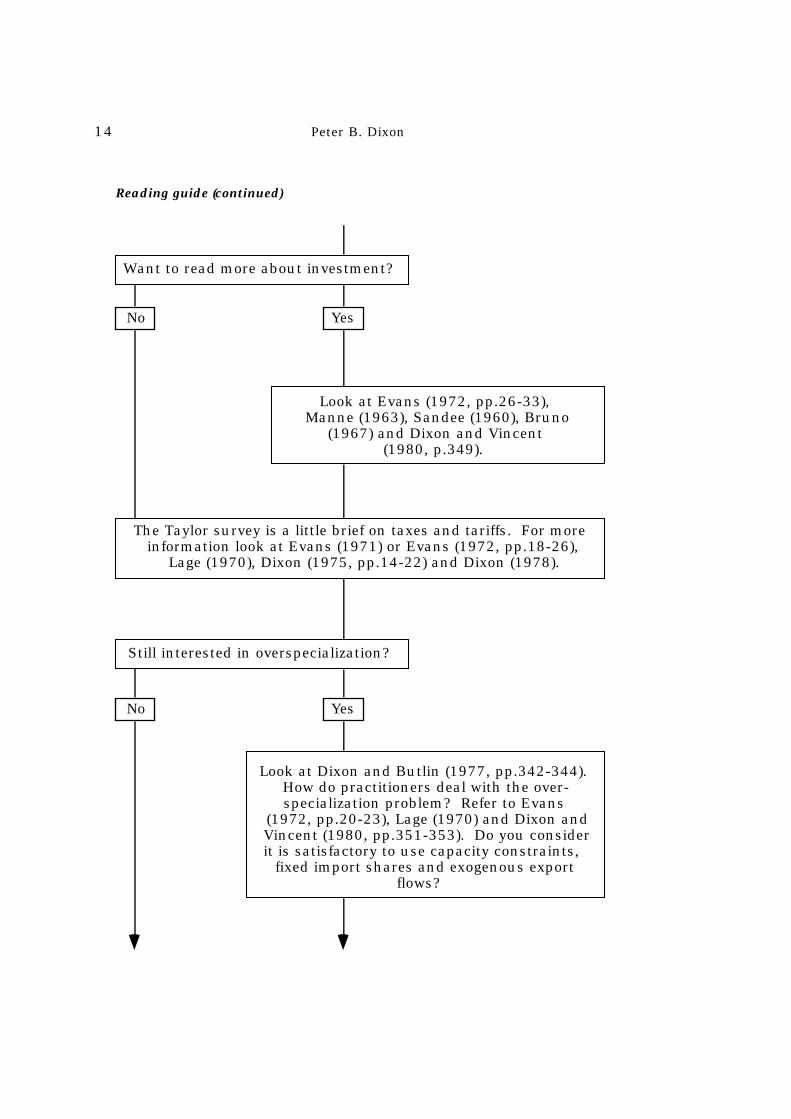
Reading guide (continued)
Read Intriligator (1971, pp.72-89). Pay particularattention to pp.79-86. This reference contains justthe right amount of detail for our purposes. Wehave also provided some brief notes emphas-
izing the idea of basic solutions in the Appendix. These notes may be sufficient if you need just a
quick reminder about linear programming.
Read Taylor (1975, pp.59-83). This reference covers the theoreticalproblems of handling investment, taxes and tariffs in the mathematicalprogramming framework. It also contains a section on the overspecial-
ization problem.
The programming problems encountered in applied general equilibriummodeling are usually of a nonlinear variety but with concave objective
functions and convex constraint sets. Approximate solutions tothese nonlinear programming problems can be obtained by solvingsuitably chosen linear programming problems. At most computer
centres, even very large linear programming problems can be solvedcheaply and conveniently. It will therefore be useful for you to knowhow nonlinear programming problems can be converted into linear
programming problems. Read Hadley (1964, pp.104-111) and/or Vajda(1961, pp.218-222).
For an elementary introduction to the idea of solving general equilibriummodels by a sequence of mathematical programming problems, readDixon (1975, pp.1-11). Earlier expositions of the relevant theory are
cited there. Of particular importance is Negishi (1960). A recentdevelopment is Manne, Chao and Wilson (1980). For straightforwardapplications of the theory see Dixon (1975, pp.22-39), Ginsburgh and
Waelbroeck (1976) and Dixon (1978).
14 Peter B. Dixon
Still interested in overspecialization?
YesNo
YesNo
Reading guide (continued)
Want to read more about investment?
Look at Evans (1972, pp.26-33),Manne (1963), Sandee (1960), Bruno
(1967) and Dixon and Vincent(1980, p.349).
The Taylor survey is a little brief on taxes and tariffs. For moreinformation look at Evans (1971) or Evans (1972, pp.18-26),
Lage (1970), Dixon (1975, pp.14-22) and Dixon (1978).
Look at Dixon and Butlin (1977, pp.342-344).How do practitioners deal with the over-specialization problem? Refer to Evans
(1972, pp.20-23), Lage (1970) and Dixon andVincent (1980, pp.351-353). Do you considerit is satisfactory to use capacity constraints,
fixed import shares and exogenous exportflows?

The Mathematical Programming Approach to Applied General Equilibrium 15
What are some of the arguments about actual economies thatmathematical programming models have been used to support?
Refer to the results and conclusions sections of some of the papersyou have already read, e.g. Evans (1971), Evans (1972, chs 5-10),
Lage (1970), Dixon and Vincent (1980) and Manne (1963). Doyou find these conclusions a worthwhile payoff for the effort
that has gone into building the models?
Review the list of goals given inthis section. Be sure you havereached them by the time you
finish your reading and problems.
Reading guide (continued)
* For full citations, see reference list for this chapter.
Exit
16 Peter B. Dixon
References
Baumol, W.J. (1972) Economic Theory and Operations Analysis, 3rdedition, Prentice-Hall.
Bruno, M. (1967) "Optimal Patterns of Trade and Development", TheReview of Economics and Statistics, Vol. 49, November, 545-554.
Corden, W.M. (1971) The Theory of Protection, Clarendon Press,Oxford.
Dixon, P.B. (1975) The Theory of Joint Maximization, North-Holland.
Dixon, P.B. (1991) “A General Equilibrium Approach to Public UtilityPricing: Determining Prices for an Urban Water Authority”,Journal of Policy Modeling.
Dixon, P.B. (1978) "The Computation of Economic Equilibria: A JointMaximization Approach", Metroeconomica, Vol. XXIX, 173-185.
Dixon, P.B., S. Bowles and D. Kendrick (DBK) (1980) Notes andProblems in Microeconomic Theory, North-Holland.
Dixon, P.B. and M.W. Butlin (1977) "Notes on the Evans Model ofProtection", Economic Record, Vol. 53 (143), June/September,337-349.
Dixon, P.B. and D.P. Vincent (1980) "Some Economic Implications ofTechnical Change in Australia to 1990-91: An IllustrativeApplication of the SNAPSHOT Model", Economic Record, Vol. 56,December, 347-361.
Evans, H.D. (1971) "Effects of Protection in a General EquilibriumFramework", Review of Economics and Statistics , Vol. 53, May,147-156.
Evans, H.D. (1972) A General Equilibrium Analysis of Protection , NorthHolland.
Gale, David (1960) The Theory of Linear Economic Models, McGraw-Hill Book Company.
Gayer, A.D., W.W. Rostow and A.J. Schwartz (1953) The Growth andFluctuation of the British Economy , 1790-1850, 2 volumes,Clarendon, Oxford.
Ginsburgh, V. and J. Waelbroeck (1976) "Computational experience witha large general equilibrium model", pp. 257-269 in J. Los and W.Los (eds), Computing Equilibria: How and Why , North-HollandPublishing Company.

The Mathematical Programming Approach to Applied General Equilibrium 17
Hadley, G. (1964) Non-Linear and Dynamic Programming, AddisonWesley.
Hazari, B.R. (1978) The Pure Theory of International Trade andDistortions, Croom-Helm Publishing Company.
Intriligator, M.D. (1971) Mathematical Optimization and EconomicTheory, Prentice-Hall.
Lage, G.M. (1970) "A Linear Programming Analysis of Tariff Protection",Western Economic Journal, Vol. viii, 167-185.
Leontief, W.W. (1978) "Issues of the coming years", Economic Impact,No. 24 (4), 70-76.
Lipsey, R.G. and K. Lancaster (1957) "The General Theory of the SecondBest", Review of Economic Studies, Vol. 24, February, 11-32.
Manne, A.S. (1963) "Key Sectors of the Mexican Economy 1960-1970",pp. 379-400 in A.S. Manne and H.M. Markowitz (eds), Studies inProcess Analysis, Wiley.
Manne, A.S., Hung-Po Chao and R. Wilson (1980) "Computation ofCompetitive Equilibria by a Sequence of Linear Programs",Econometrica, Vol. 48 (7), November, 1595-1616.
Negishi, T. (1960) "Welfare Economics and the Existence of anEquilibrium for a Competitive Economy", Metroeconomica, Vol.XII, 92-97.
Samuelson, P.A. (1950) "Evaluation of Real National Income", OxfordEconomic Papers, Vol. 2 (NS), January, 1-29.
Sandee, J. (1960) A Long-term Planning Model for India, Asia PublishingHouse, New York and Statistical Publishing Company, Calcutta.
Sauvy, Alfred (1969) General Theory of Population, Weidenfeld andNicholson, London
Taylor, L. (1975) "Theoretical Foundations and Technical Implications",pp. 33-109 in C.R. Blitzer, P.B. Clark and L.Taylor (eds), Economy-Wide Models and Development Planning, Oxford University Press.
Vajda, S. (1961) Mathematical Programming, Addison-Wesley PublishingCompany.
18 Peter B. Dixon
Exercise 1 The implications of technical change in a wine-clotheconomy
This is an easy warm-up exercise. It uses a very elementarymodel to introduce a few important general equilibrium ideas withoutalgebraic complications. It is organized in four sections. The firstdescribes the net annual production possibilities set, i.e., what can beproduced with existing techniques and resources in one year. Thesecond introduces consumer preferences to determine what will beproduced. In the third we discuss prices and real wages. In the lastsection we are ready to derive the implications of a change inproduction techniques.
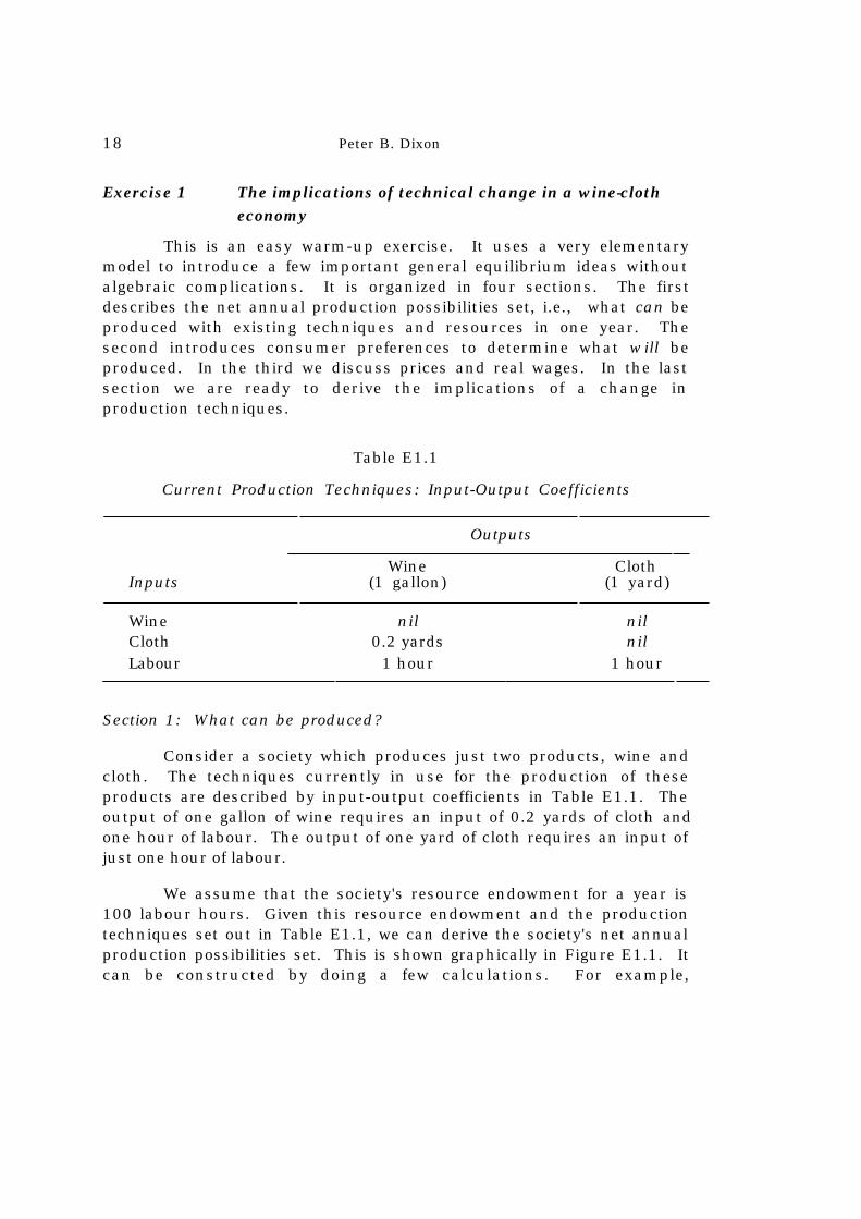
Table E1.1
Current Production Techniques: Input-Output Coefficients
Outputs
Wine ClothInputs (1 gallon) (1 yard)
Wine nil nilCloth 0.2 yards nilLabour 1 hour 1 hour
Section 1: What can be produced?
Consider a society which produces just two products, wine andcloth. The techniques currently in use for the production of theseproducts are described by input-output coefficients in Table E1.1. Theoutput of one gallon of wine requires an input of 0.2 yards of cloth andone hour of labour. The output of one yard of cloth requires an input ofjust one hour of labour.
We assume that the society's resource endowment for a year is100 labour hours. Given this resource endowment and the productiontechniques set out in Table E1.1, we can derive the society's net annualproduction possibilities set. This is shown graphically in Figure E1.1. Itcan be constructed by doing a few calculations. For example,
The Mathematical Programming Approach to Applied General Equilibrium 19
100
40
A
E1
0
50 100
B
-20D
Net output ofwine (gallons)
Net output ofcloth (yards)
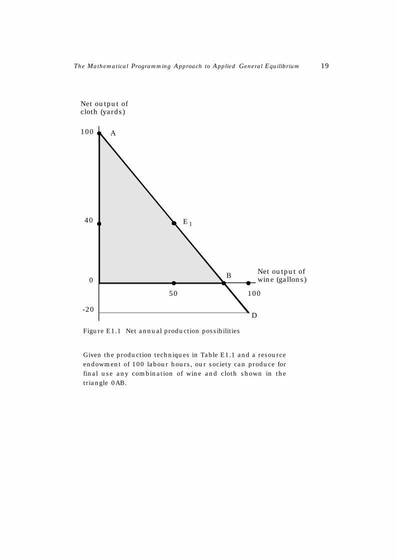
Figure E1.1 Net annual production possibilities
Given the production techniques in Table E1.1 and a resourceendowment of 100 labour hours, our society can produce forfinal use any combination of wine and cloth shown in thetriangle 0AB.
20 Peter B. Dixon
if 50 labour hours were devoted to wine and 50 to cloth, then society'snet annual output would be 50 gallons and 40 yards. Notice that the grossoutput of cloth is 50 yards, but that 10 yards are used up in wineproduction. We have marked the point 50 gallons and 40 yards as E1 inFigure E1.1. Now consider the case in which our society allocates all itsresources (100 labour hours) to cloth production. Net annual outputwould be 100 yards of cloth and no wine (point A in Figure E1.1). Onthe other hand, if all the labour were devoted to wine, we would end upwith 100 gallons, but we would have a deficit of 20 yards of cloth (pointD in Figure E1.1). Perhaps the deficit could be made up by drawing onaccumulated stocks or through importing. But for simplicity we willassume that there are no accumulated stocks and that there is nointernational trade. Thus, the net annual production possibilities avail-able to our society are restricted to the shaded area 0AB in Figure E1.1.
(a) Can our society produce a net annual output of 40 gallons of wineand 60 yards of cloth?
(b) Can our society produce a net annual output of 40 gallons of wineand 30 yards of cloth?
(c ) Consider the production techniques shown in Table E1.2. Theonly change from those in Table E1.1 is in the labour inputcoefficient for cloth. Technical progress has taken place whichallows a yard of cloth to be produced with only 0.5 hours oflabour input rather than one hour. Assume that the society'sresource endowment remains at 100 labour hours per year. Canyou construct the new net annual production possibilities set?
Table E1.2Production Techniques after an Improvement
in the Technique for Producing Cloth
Wine Cloth(1 gallon) (1 yard)
Wine nil nil
Cloth 0.2 yards nil
Labour 1 hour 0.5 hours
The Mathematical Programming Approach to Applied General Equilibrium 21
Section 2: What will be produced?
Having constructed society's net annual production possibilitiesset and illustrated it in Figure E1.1, our next task is to determine whichpoint in the set will be chosen. This will depend on (i) the level ofemployment and (ii) consumer preferences for wine and cloth.
Let us make the assumption that our society achieves fullemployment, i.e., all of the 100 labour hours are used in production.This contentious assumption is discussed in some detail in the final partof this exercise. If we accept the full employment assumption, then wecan restrict our search for the actual net production point to thefrontier, AB, of the net annual production possibilities set. It is only onthe frontier that we have full employment.
Which point will be chosen on the frontier, AB? This willdepend on what society wants to consume. Let us consider the simplestpossible case by assuming that our society always consumes wine andcloth in fixed proportions: 5 gallons of wine to 4 yards of cloth. Interms of Figure E1.2, consumption will occur somewhere along the line0C. In fact, in view of our full employment assumption, we can see thatnet production and consumption of wine and cloth will be 50 gallonsand 40 yards (point E1 in Figure E1.2).
(d ) At E1 how many labour hours will be used in the production ofwine? How many will be used in the production of cloth?
(e ) Continue to assume that total employment is 100 labour hoursand that wine and cloth are consumed in the ratio of 5 gallons to4 yards. If the production technique for cloth improves to thatshown in Table E1.2, what will be the new levels for netproduction and consumption of wine and cloth? How manylabour hours will be used in wine production? How many incloth production?
Section 3: Commodity prices and real wages
At this stage we have come a long way. Starting from a de -scription of production techniques and consumer preferences, we havefound out what our society will produce and consume, and what

22 Peter B. Dixon
employment will be in each industry. We can also determine com-modity prices and the real hourly wage rate.8
Suppose that the nominal wage rate is $1 per hour. Then underthe production techniques shown in Table E1.1, the price of clothwould be $1 per yard. This is because it takes one hour of labour tomake a yard of cloth. The price of a gallon of wine would be $1.2, i.e.,the cost of one hour of labour plus the cost of 0.2 yards of cloth. Thehourly wage ($1) would be just sufficient to buy a commodity bundlecontaining 0.5 gallons of wine and 0.4 yards of cloth.
(f) If the wage rate were $10 per hour, what would be the prices ofwine and cloth? Would the wage for an hour's labour still buy acommodity bundle containing 0.5 gallons of wine and 0.4 yardsof cloth? In determining the real hourly wage rate, does it makeany difference whether we assume the nominal hourly wage is$1 or $10?
(g) Assume that the wage rate is $1 per hour and that theproduction techniques are those shown in Table E1.2. What willbe the prices of wine and cloth? Check that the wage for anhour's labour can now buy a commodity bundle containing 0.67gallons of wine and 0.53 yards of cloth.
Section 4: The effects of a change in production techniques
In Table E1.3 we have listed everything that we have found outabout the economy of our wine-cloth society. Column I showscommodity outputs, employment in each industry, commodity pricesand the real wage rate in the initial situation (i.e., when the productiontechniques are those in Table E1.1). Column II shows thecorresponding results when the production techniques are those inTable E1.2. By comparing columns I and II, we can see the economy-wide effects of the improvement in the production technique for cloth.The halving of the labour input coefficient to cloth production hasallowed consumption and net production of both wine and cloth toincrease by 331
3 per cent, real wage rates to increase by 3313 per cent,
8 The real hourly wage rate is measured by a quantity of commodities thatcan be purchased in return for one hour's labour.

The Mathematical Programming Approach to Applied General Equilibrium 23
Table E1.3
The Wine-Cloth Economy before and after the Improvementin the Technique for Producing Cloth
I. Before II. After
Net annual output andconsumption
Wine 50 gallons 6623 gallons
Cloth 40 yards 5313 yards
Employment
Wine 50 hours 6623 hours
Cloth 50 hours 3313 hours
Prices (assuming that
the wage rate is $1 per hour)
Wine $1.2 per gallon $1.1 per gallon
Cloth $1.0 per yard $0.5 per yard
Real wage rate
The wage for 0.5 gallons 0.67 gallons
one hour’s plus plus
labour buys 0.4 yards 0.53 yards
the price of cloth to fall sharply relative to that of wine and 1623 per cent
of the labour force to be reallocated from the cloth industry to the wineindustry.
This analysis is quite similar to that used by economistsconcerned with quantifying the effects of technical change in the realworld. For example, in their study of the Australian economy, Dixon andVincent (1980) assembled two tables of input-output coefficients, one
24 Peter B. Dixon
showing production techniques as they were in 1971/72 and the othershowing the production techniques forecast for 1990/91.9 They thenmade some comparisons. Their central computation was designed toanswer the following question: how much difference do the projectedchanges in production techniques make to one's picture of how theeconomy will be in 1990/91. In terms of Figures E1.2 and E1.3, Dixonand Vincent computed the points E1 and E2, where E1 refers to thelevels which would be achieved in 1990/91 for commodity outputs,prices, real wages, etc., if production techniques remained as they werein 1971/72 and E2 refers to the situation which will emerge ifproduction techniques are consistent with the forecasts. Thecomparison between E1 and E2 was, therefore, the basis for a discussionof the implications of technical change.
Dixon and Vincent had to consider many details which were notincluded in our wine-cloth economy. They divided the economy into109 sectors, rather than 2. They included capital, not just labour as aprimary factor of production and they divided labour into 9 occupationalgroups. They considered the role of investment, not just consumption.They allowed for international trade, government expenditure andnumerous taxes, tariffs and subsidies. Nevertheless, in essence, theirapproach consisted of the steps outlined in this exercise: (i) thederivation of alternative net annual production possibilities setscorresponding to alternative assumptions about production techniques,and (ii) the imposition of the full employment assumption and theconsideration of consumer preferences leading to the calculation of thenet production points.
What did Dixon and Vincent conclude from their study? Giventhe preliminary nature of their work and a number of deficiencies whichthey were careful to emphasize, they were cautious. They did, however,offer the following:
9 The forecasts were based on work done by two agencies sponsored by theAustralian Government: the Bureau of Industry Economics (BIE) and theIMPACT Project. The BIE selected industries which appeared to beundergoing rapid technical change and asked industry experts to forecastthe future input-output coefficients. Where expert opinions were notavailable, forecasts based on trend projections were prepared by theIMPACT Project.

The Mathematical Programming Approach to Applied General Equilibrium 25
66.7
40
50 0 100
-20
C
B
D
A
100
40
0 50 100
-20
A
C
B
D
Net output ofcloth (yards)
Net output ofcloth (yards)
Net outputof wine(gallons)
Net outputof wine(gallons)
E1
E253.3
Figure E1.2 Net annualproduction possibilities underthe ini t ia l product iontechniques
Apart from the addition of theconsumption line, 0C, thisfigure is the same as FigureE1.1.
Figure E1.3 Net annualproduction possibilities afterthe improvement in thetechnique for producingcloth

26 Peter B. Dixon
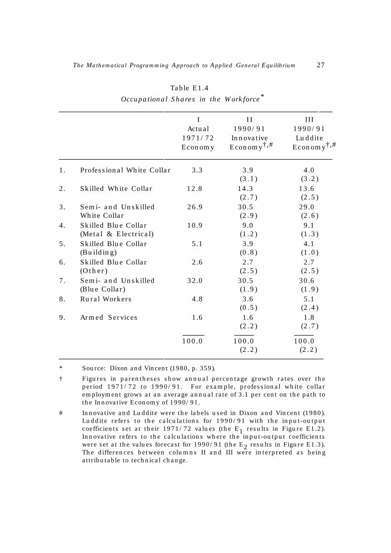
"The overwhelming impression from Table 4.6 [reproduced hereas Table E1.4] is that the occupational composition of the workforceat the 9-order level in 1990/91 is unlikely to be radically differentfrom that in 1971/72 and that it will be determined largelyindependently of technical change. Certainly, the presentsimulations do not pinpoint any likely difficulties in the areas oflabour mobility and manpower training." [Dixon and Vincent (1980,p. 358)]
and
"Subject to the qualifications expressed throughout the paper, ourresults indicate that rapid technical progress is particularlyimportant for the future well-being of those Australian industrieswhich are closely connected with international trade. At the macrolevel, our results support the view that technical progress is vital forsecuring increased GDP, increased consumption and higher realwages. Technical progress may also affect macro economicmanagement. In the absence of technical progress, we found thatthe 'full-employment' level of real wages would decline. Under suchconditions, it is difficult to imagine that Australia could achieve evena tolerable approximation to full employment." [Dixon and Vincent(1980, p. 359)]
(h) In Table E1.4, you will see references to innovative and Ludditeeconomies. Who were the Luddites?
The calculations by Dixon and Vincent and our own analysis ofthe wine-cloth economy present technical change in a favourable light.Only its role as a source of increased material welfare is emphasized.But this is not the aspect of technical change which has always beenemphasized in popular discussions. Sometimes, the principal concernhas been with job replacement. Newspapers frequently report fearsexpressed by various groups in the community concerning theemployment effects of new machines: word-processors, automatic banktellers, point-of-sale terminals, vending machines and robots.
Let us re-examine our wine-cloth story from the point of view ofthe employment implications of technical change. The critical assump-tion in the story is that technical change is not an important determi-nant of the aggregate level of employment. It is assumed that aggregateemployment is 100 labour hours both before and after the improvementin the production technique for cloth. There is no need to assume that
The Mathematical Programming Approach to Applied General Equilibrium 27
Table E1.4
Occupational Shares in the Workforce*
I I I III Actual 1990/91 1990/91
1971/72 Innovative LudditeEconomy Economy†,# Economy†,#
1. Professional White Collar 3.3 3.9 4.0(3.1) (3.2)
2. Skilled White Collar 12.8 14.3 13.6(2.7) (2.5)
3. Semi- and Unskilled 26.9 30.5 29.0White Collar (2.9) (2.6)
4. Skilled Blue Collar 10.9 9.0 9.1(Metal & Electrical) (1.2) (1.3)
5. Skilled Blue Collar 5.1 3.9 4.1(Building) (0.8) (1.0)
6. Skilled Blue Collar 2.6 2.7 2.7(Other) (2.5) (2.5)
7. Semi- and Unskilled 32.0 30.5 30.6(Blue Collar) (1.9) (1.9)
8. Rural Workers 4.8 3.6 5.1(0.5) (2.4)
9. Armed Services 1.6 1.6 1.8(2.2) (2.7)
100.0 100.0 100.0
(2.2) (2.2)
* Source: Dixon and Vincent (1980, p. 359).
† Figures in parentheses show annual percentage growth rates over theperiod 1971/72 to 1990/91. For example, professional white collaremployment grows at an average annual rate of 3.1 per cent on the path tothe Innovative Economy of 1990/91.
# Innovative and Luddite were the labels used in Dixon and Vincent (1980).Luddite refers to the calculations for 1990/91 with the input-outputcoefficients set at their 1971/72 values (the E1 results in Figure E1.2).Innovative refers to the calculations where the input-output coefficientswere set at the values forecast for 1990/91 (the E2 results in Figure E1.3).The differences between columns II and III were interpreted as beingattributable to technical change.

28 Peter B. Dixon
employment of 100 labour hours is literally full employment. Perhaps 105hours of labour are available. Our assumption is that 5 per centunemployment is just as likely with technical progress as without it.10
This assumption should not be too surprising to readers withsome knowledge of conventional macroeconomic theory. That theorystresses demand management, fiscal and monetary policy and the realwage rate in relation to labour productivity as the major determinants ofaggregate employment. The rate of technical change rarely rates even amention. This will not be very reassuring to readers who are scepticalabout conventional economic theory. They will want us to spell out theprocess by which workers, displaced by technical change, will find newjobs.
In terms of our wine-cloth economy, the problem is to explainthe transition from E1 to E2 (Figures E1.2 and E1.3). Starting at E1, thehalving of the labour input coefficient for cloth will mean that only 25labour hours (rather than 50) are required in the industry. Cloth nowwill be cheaper and the real incomes of employed workers will expand.These workers will demand more wine and cloth, thus providingemployment for the previously displaced workers. This will set us onthe happy path to E2.
What if capitalists prevent the reduction in the real price ofcloth by taking an increase in profits? But don't capitalists consumewine and cloth too? Perhaps not, perhaps capitalists spend onimported luxuries and overseas holidays. But what will the foreigners dowith the domestic dollars they receive from the capitalists? They willbuy our wine and cloth! But what happens if everyone has had enoughwine and cloth? This would be a blissful state — we could simply do lesswork. Unfortunately a state in which all our material wants are satisfiedseems very far away, even in the world's wealthiest countries.
What about adjustment problems along the path from E1 to E2?Recall that the shift from E1 to E2 involved the transfer of 162
3 per centof the labour force out of cloth and into wine. What if the skills requiredof wine workers differ from those of cloth workers? Then might not
10 This assumption may be overly generous to the situation with no technicalprogress. With no technical progress there is unlikely to be scope forincreases in real wages without reductions in employment.
The Mathematical Programming Approach to Applied General Equilibrium 29
the move from E1 to E2 cause excessive periods of unemployment forsurplus cloth workers? Certainly this is a possibility. It is important,therefore, in comparing E1 and E2 to consider the feasibility of theimplied rates of shift of resources between different activities. This iswhat Dixon and Vincent did in their analysis of the implications oftechnical change to 1990/91. For example, on examining Table E1.4,they concluded that technical change to 1990/91 could be accom-modated without rapid transfers of labour between the nine broadlydefined occupational groups. It is possible, however, that technicalchange to 1990/91 may render redundant certain very specific skills.This does not necessarily imply any serious difficulties. In manycountries, workers exhibit a high degree of occupational mobility.
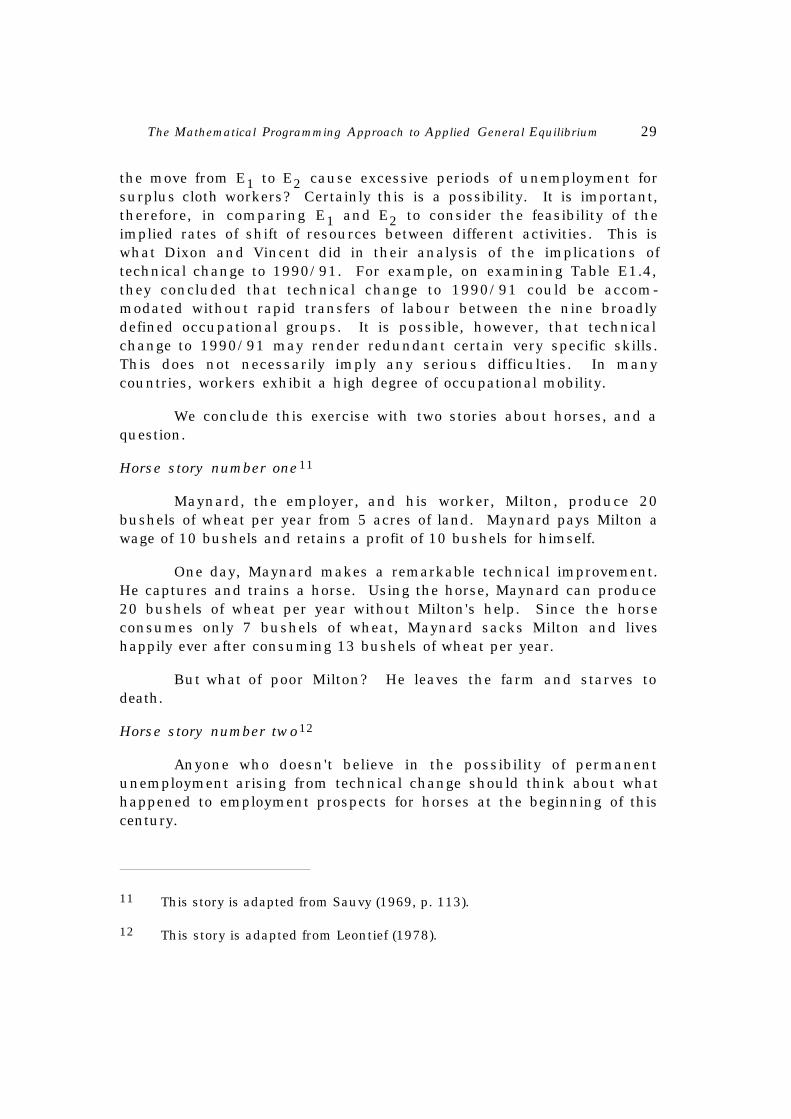
We conclude this exercise with two stories about horses, and aquestion.
Horse story number one11
Maynard, the employer, and his worker, Milton, produce 20bushels of wheat per year from 5 acres of land. Maynard pays Milton awage of 10 bushels and retains a profit of 10 bushels for himself.
One day, Maynard makes a remarkable technical improvement.He captures and trains a horse. Using the horse, Maynard can produce20 bushels of wheat per year without Milton's help. Since the horseconsumes only 7 bushels of wheat, Maynard sacks Milton and liveshappily ever after consuming 13 bushels of wheat per year.
But what of poor Milton? He leaves the farm and starves todeath.
Horse story number two12
Anyone who doesn't believe in the possibility of permanentunemployment arising from technical change should think about whathappened to employment prospects for horses at the beginning of thiscentury.
11 This story is adapted from Sauvy (1969, p. 113).
12 This story is adapted from Leontief (1978).

30 Peter B. Dixon
(i) Have either of these horse stories any relevance to the analysis ofthe implications of technical change in a modern economy?Both imply the possibility of an unhappy outcome from technicalchange. What are the key differences in the assumptionsunderlying our wine-cloth analysis and the assumptionsunderlying the horse stories?
Answer to Exercise 1
(a) No. In terms of Figure E1.1, the point 40 gallons, 60 yards liesoutside the triangle 0AB. Given the production techniques in TableE1.1, it would take a gross output of 40 gallons and 68 yards to achieve anet output of 40 gallons and 60 yards. Thus, 108 hours of labour wouldbe required. Only 100 hours are available.
(b) Yes. In terms of Figure E1.1, the point 40 gallons, 30 yards isinside the triangle 0AB. Given the production techniques in Table E1.1,it would take a gross output of 40 gallons and 38 yards to achieve a netoutput of 40 gallons and 30 yards. Thus, 78 hours of labour would berequired. This is available.
(c) The new net annual production possibilities set is shown inFigure E1.3 as the triangle 0AB. It can be constructed by consideringthe net outputs which would emerge as we vary the allocation of labourbetween the production of our two commodities. For example, if all the100 labour hours were devoted to cloth production, then we wouldobtain 200 yards of cloth and no wine. Hence point A in Figure E1.3 ispart of the new net annual production possibilities set. If 662
3 hours oflabour were devoted to wine and 331
3 to cloth, then net productionwould be 662
3 gallons of wine and 5313 yards of cloth, point E2 in Figure
E1.3. (Notice that the use of 3313 labour hours in cloth generates a gross
output of 6623 yards, but that the wine production uses up 131
3 (= 0.2 ×662
3 yards.) If 100 labour hours were devoted to wine production, thenwe would obtain 100 gallons. There would, however, be a deficit of 20yards of cloth. (See point D in Figure E1.3.) Because we rule out bothinternational trade and the existence of accumulated stocks, deficits arenot possible. Hence the net annual production possibilities are confinedto the triangle 0AB in Figure E1.3.
Be sure to compare the new net annual production possibilitiesset with the old one. As can be seen by looking at Figures E1.2 andE1.3, technical progress in the cloth industry leads to an expansion ofthe possibilities set.

The Mathematical Programming Approach to Applied General Equilibrium 31
(d) At E1, the gross outputs are 50 gallons of wine and 50 yards ofcloth. Hence 50 labour hours are used in wine production and 50 incloth production.
(e) In Figure E1.3, the consumption line 0C crosses the frontier ofthe net annual production possibilities set at E2. The levels for netproduction and consumption of wine and cloth are 662
3 gallons and 5313
yards. Employment is 6623 hours in wine and 331
3 hours in cloth.
(f) If the wage rate were $10 per hour, the price of cloth would be$10 per yard and the price of wine would be $12 per gallon. The realwage rate would be unaffected by an increase in the wage rate from $1per hour to $10 per hour. In both cases, the wage for an hour's labourwould buy a bundle of commodities containing 0.4 yards of cloth and 0.5gallons of wine.
(g) The price of cloth will be $0.5 per yard and the price of winewill be $1.1 per gallon. At these prices, a commodity bundle containing0.67 gallons of wine and 0.53 yards of cloth would cost $1, i.e., thewage for one hour of labour would buy a bundle containing 0.67 gallonsof wine and 0.53 yards of cloth.
(h) The Luddites were organized bands of English workmen who in1811-12 destroyed stocking frames, steam power looms and shearingmachines in various centres of the British textile industry. A popularbelief at the time was that these recently introduced labour-savingmachines were a cause of low real wages and high unemployment.Luddite activity again broke out in 1816.
It is doubtful that technical advances taking place in the Britishtextile industry in the early 19th century had anything to do with theparticularly miserable position of British workers in 1811-12 and 1816.In both these years the British economy was in a state of recessionarising from poor harvests and high food prices. By blaming technicalprogress (machines), the workers appear to have misidentified thesource of their problems. See, for example, Gayer, Rostow andSchwartz (1953, pp. 135-7).
(i) The key differences between the assumptions underlying thehorse stories and those underlying the wine-cloth story concern humanadaptability to change. In the wine-cloth story, the displaced clothworkers can move into wine production. By contrast, horse storynumber one depicts the displaced worker, Milton, as having no viablealternative to working for Maynard. One wonders why Milton does not
32 Peter B. Dixon
capture a horse and work some land of his own. Perhaps society hasadvanced to the stage where all the arable land is occupied. But then itis surprising that Milton does not go to a town and work in an urbanoccupation. Horse story number two also depicts the possibility of thedisplaced workers being left with nothing to do, the displaced workersthis time being horses. We should note, however, that the horses whichlost their jobs at the turn of the century had a very limited range ofskills compared with human workers.
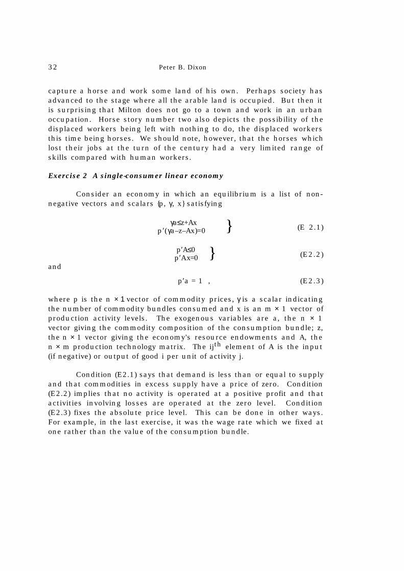
Exercise 2 A single-consumer linear economy
Consider an economy in which an equilibrium is a list of non-negative vectors and scalars {p, γ, x} satisfying
}γa≤z+Axp′(γa–z–Ax)=0 (E 2.1)
}p′A≤0p′Ax=0 (E2.2)
and
p′a = 1 , (E2.3)
where p is the n × 1 vector of commodity prices, γ is a scalar indicatingthe number of commodity bundles consumed and x is an m × 1 vector ofproduction activity levels. The exogenous variables are a, the n × 1vector giving the commodity composition of the consumption bundle; z,the n × 1 vector giving the economy's resource endowments and A, then × m production technology matrix. The ijth element of A is the input(if negative) or output of good i per unit of activity j.
Condition (E2.1) says that demand is less than or equal to supplyand that commodities in excess supply have a price of zero. Condition(E2.2) implies that no activity is operated at a positive profit and thatactivities involving losses are operated at the zero level. Condition(E2.3) fixes the absolute price level. This can be done in other ways.For example, in the last exercise, it was the wage rate which we fixed atone rather than the value of the consumption bundle.

The Mathematical Programming Approach to Applied General Equilibrium 33
(a) Assume that
a =
5
4
0
, z =
0
0
100
and A =
1.0 0.0
–0.2 1.0
–1.0 –1.0
.
What are the equilibrium values for p, γ and x? If we let thethree commodities be wine, cloth and labour, then (apart fromthe choice for the absolute price level) the present model is thesame as that in Exercise 1 before the improvement in thetechnology for making cloth.
(b) Assume that a new technique for producing commodity 2becomes available. The economy's production technology matrixis now
A =
1.0 0.0 –0.1
–0.2 1.0 1.1
–1.0 –1.0 –1.0
Will the new technique be used?
(c ) In special cases where the numbers of commodities, n, andactivities, m, are small, it is possible to solve the model (E2.1) –(E2.3) by elementary graphical and/or algebraic methods. Inempirically interesting cases, where n and m may be large, thesemethods are not adequate. Write down a linear programmingproblem which would be a suitable vehicle for solving (E2.1) –(E2.3).
Answer to Exercise 2
(a) In this economy, activity 1 is the only method for producingcommodity 1 and activity 2 is the only method for producing commodity2. It is clear, therefore, that both activities must be operated at positivelevels. Thus, we can find the equilibrium prices from
(p1, p2, p3)
1.0 0.0
–0.2 1.0
–1.0 –1.0
= (0,0)
and

34 Peter B. Dixon
5p1 + 4p2 = 1 .
This gives
(p1, p2, p3) = (0.12, 0.10, 0.10) .
Because all prices are positive, we know that the market clearingconditions hold as equalities. Thus, we can determine γ, x1 and x2 from
γ
5
4
0
=
0
0
100
+
1.0 0.0
–0.2 1.0
–1.0 –1.0
x1
x2
,
that is
–1.0 0.0 5
0.2 –1.04
1.0 1.0 0
x1
x2
γ
=
0
0
100
. (E2.4)
On solving equation (E2.4) we obtain
x1 = 50, x2 = 50 and γ = 10 .
(b) Because activity 1 continues to be the only method for producingcommodity 1, we may assume that it is still operated at a positive level.If the new activity (activity 3) were also operated at a positive level, thecommodity prices would satisfy
(p1, p2, p3)
1.0 –0.1
–0.2 1.1
–1.0 –1.0
= (0, 0)
and
5p1 + 4p2 = 1 ,
giving
(p1, p2, p3) = (0.1193, 0.1009, 0.0991) . (E2.5)
At these prices, the profit per unit of activity 2 is
The Mathematical Programming Approach to Applied General Equilibrium 35
(0.1193, 0.1009, 0.0991)
0.0
1.0
–1.0
= 0.0018 > 0 .
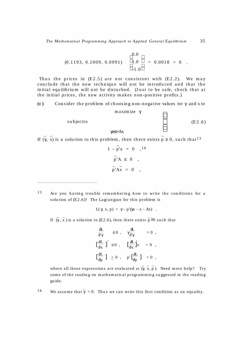
Thus the prices in (E2.5) are not consistent with (E2.2). We mayconclude that the new technique will not be introduced and that theinitial equilibrium will not be disturbed. (Just to be safe, check that atthe initial prices, the new activity makes non-positive profits.)
(c) Consider the problem of choosing non-negative values for γ and x to
maximize γ
subjectto
γa≤z+Ax.
(E2.6)
If (γ_, x
_) is a solution to this problem, then there exists p
_ ≥ 0, such that13
1 – p_
′a = 0 ,14
p_
′A ≤ 0 ,
p_
′Ax_ = 0 ,
13 Are you having trouble remembering how to write the conditions for a
solution of (E2.6)? The Lagrangian for this problem is
L( γ, x, p) = γ – p′(γa – z – Ax) .
If (γ_ , x
_ ) is a solution to (E2.6), then there exists p
_ ≥0 such that
∂L∂ γ ≤ 0 , γ
∂L∂ γ = 0 ,
[ ∂L∂x
] ′ ≤ 0 , [ ∂L∂x ]′x = 0 ,
[ ∂L∂p
] >_ 0 , p′ [ ∂L∂p ] = 0 ,
where all these expressions are evaluated at (γ_, x
_, p
_ ). Need more help? Try
some of the reading on mathematical programming suggested in the reading
guide.
14 We assume that γ_ > 0. Thus we can write this first condition as an equality.

36 Peter B. Dixon
γ_a ≤ z + Ax
_
andp_
′( γ_a – z – Ax
_) = 0 .
Thus solutions for models of the form (E2.1) – (E2.3) may be computedby solving linear programming problems of the form (E2.6). Thesolution (γ
_, x
_) to (E2.6), together with the associated Lagrangian
multipliers or dual solution (p_), satisfies the conditions (E2.1) – (E2.3).
Exercise 3 The utility possibilities frontier
When we move from single-consumer to multiple-consumermodels, the utility possibilities frontier becomes a useful concept. As isapparent from subsequent exercises, it is sometimes convenient to solvemultiple-consumer models by searching the utility possibilities frontier.
In the context of an r-consumer model with a given specificationof resource endowments, production technologies and external tradingopportunities, the vector of utility levels U ≡ (U1, U2, ...,Ur) is a point onthe utility possibilities frontier if and only if U is feasible and
U_
i < Ui for at least one i
if U_
≡ (U_
1,...,U_
r) is a feasible utility vector different from U. (U and U_
are feasible if it is possible to generate the consumption levels requiredto support them.)
In some cases, we can describe the utility possibilities frontierby an equation of the form
f(U1,U2, ...,Ur) = 0 (E3.1)
where (U1,...,Ur) is a point on the utility possibilities frontier if and onlyif it satisfies (E3.1).
(a) Consider a two-consumer, two-commodity pure exchange model(no production) where the utility functions for the two con-sumers are
Ui = (C i1)1/2
(C i2)1/2
, i =1,2 (E3.2)
and where Cij is the consumption of good j by consumer i.Assume that the consumers' endowment vectors are
The Mathematical Programming Approach to Applied General Equilibrium 37
Z′1 = (100, 0)
andZ′
2 = (0, 100) .
Derive the equation for the utility possibilities frontier andprovide a sketch of the utility possibilities set.
(b) Answer question (a) with (E3.2) replaced by
Ui = (C i1)1/4
(C i2)1/4
, i=1,2 . (E3.3)
(c ) Answer question (a) with (E3.2) replaced by
U1 = (C 11)1/4
(C 12)1/4
(E3.4)
and
U2 = (C 21)1/2
(C 22)1/2
. (E3.5)
(d) Answer question (a) with (E3.2) replaced by
Ui = ln(Cil) + ln(Ci2) , i=1,2 . (E3.6)
(e ) Show that for an r-consumer, pure exchange model, the utilitypossibilities set is convex if the utility functions are concave.
(f) Generalize part (e). Assume that the net production possibilitiesset is convex. Show that the utility possibilities set is convex ifthe utility functions are concave.
Answer to Exercise 3
(a) Let (U1, U2) be a point on the utility possibilities frontier withC′
1 ≡ (C11, C12) and C′2 ≡ (C21, C22) being the underlying consumption
vectors. Then
U1 = (C 11)1/2
(C 12)1/2
, (E3.7)
U2 = (C 21)1/2
(C 22)1/2
, (E3.8)
C11 + C21 = Z11 + Z21 = 100 (E3.9)
and
38 Peter B. Dixon
C12 + C22 = Z12 + Z22 = 100 . (E3.10)
We also know that the marginal rate of substitution between goods 1 and2 will be the same for consumer 1 as for consumer 2. If this conditionwere not satisfied, it would be possible to raise the utility levels of bothconsumers by reallocating commodities between them. Thus,
∂U1(C1)
∂C11 /
∂U1(C1)
∂C12 =
∂U2(C2)
∂C21 /
∂U2(C2)
∂C22 . (E3.11)
Under (E3.2), (E3.11) implies that
C12C11
= C22C21
. (E3.12)
To derive the utility possibilities frontier, we eliminate the four Cijsfrom the five equations (E3.7) – (E3.10) and (E3.12) leaving useventually with an equation of the form f(U1, U2) = 0. As the first stepin the algebra we note that (E3.7) and (E3.8) imply that
U1 U2 = (C11)1/2 (C22)1/2 (C21)1/2(C12)1/2 . (E3.13)
On using (E3.12) in (E3.13), we obtain
U1 U2 = C11 C22 = C21 C12 (E3.14)
Next, we use (E3.9) and (E3.10) to find that
C11 C12 + C12 C21 + C11 C22 + C21 C22 = 10,000 . (E3.15)
Substitution into (E3.15) from (E3.7), (E3.8) and (E3.14) gives
U21 + 2U1U2 + U
22 = 10,000 ,
that is
(U1 + U2)2 – 10,000 = 0 . (E3.16)
In view of (E3.7) and (E3.8) we can assume that U1 and U2 are non-negative. Thus, we may write the equation to the utility possibilitiesfrontier as

The Mathematical Programming Approach to Applied General Equilibrium 39
U1 + U2 – 100 = 0 . (E3.17)
The utility possibilities set is illustrated in Figure E3.1(a).
(b) We start by replacing (E3.7) and (E3.8) by
U2i = (Ci1)1/2
(Ci2)1/2 , i=1,2 .
(E3.9), (E3.10) and (E3.12) remain valid. Thus, we can follow the stepsin part (a), replacing Ui wherever it appears with U
2i . Consequently, it
follows from (E3.17) that the equation for the utility possibilitiesfrontier is
U21 + U
22 – 100 = 0 . (E3.18)
The utility possibilities set is illustrated in Figure E3.1(b).
(c) We replace (E3.7) by
U21 = (C11)1/2
(C12)1/2 .
(E3.8), (E3.9), (E3.10) and (E3.12) remain valid. It follows from part (a)that the equation for the utility possibilities frontier is
U21 + U2 – 100 = 0 .
The utility possibilities set is illustrated in Figure E3.1(c).
(d) Equation (E3.6) can be rewritten as
[e Ui]1/2
= (Ci1)1/2 (Ci2 )1/2 , i=1, 2 .
(E3.9), (E3.10) and (E3.12) remain valid. Thus, from part (a) we canconclude that the equation to the utility possibilities frontier is

40 Peter B. Dixon
1U
2 U
0 10
100
0 0 100 10
100 10
Figure E3.1(a) Figure E3.1(b)
Figure E3.1(c)
9.210
9.210
Figure E3.1(d)
1U 1U
2 U 2 U
+ U - 100 = 02U1 + U - 100 = 022
U12
+ U - 100 = 02U12
] - 100 = 01/2[eUi 2
i=1Σ
1U
2 U
0
Figure E3.1 Utility possibilities frontiers
Utility possibilities sets are indicated by shading.
The Mathematical Programming Approach to Applied General Equilibrium 41
Σi=1
2
[e Ui]1/2
– 100 = 0 .
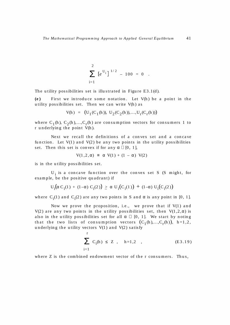
The utility possibilities set is illustrated in Figure E3.1(d).
(e) First we introduce some notation. Let V(h) be a point in theutility possibilities set. Then we can write V(h) as
V(h) = (U1(C1(h)), U2(C2(h)),...,Ur(Cr(h)))
where C1(h), C2(h),...,Cr(h) are consumption vectors for consumers 1 tor underlying the point V(h).
Next we recall the definitions of a convex set and a concavefunction. Let V(1) and V(2) be any two points in the utility possibilitiesset. Then this set is convex if for any α ∈ [0, 1],
V(1,2,α) ≡ α V(1) + (1 – α ) V(2)
is in the utility possibilities set.
U i is a concave function over the convex set S (S might, forexample, be the positive quadrant) if
Ui(α Ci(1) + (1–α) Ci(2)) >_ α Ui(Ci(1)) + (1–α) Ui(Ci(2))
where Ci(1) and Ci(2) are any two points in S and α is any point in [0, 1].
Now we prove the proposition, i.e., we prove that if V(1) andV(2) are any two points in the utility possibilities set, then V(1,2,α) isalso in the utility possibilities set for all α ∈ [0, 1]. We start by notingthat the two lists of consumption vectors (C1(h),...,Cr(h)), h=1,2,underlying the utility vectors V(1) and V(2) satisfy
Σi=1
r
Ci(h) ≤ Z , h=1,2 , (E3.19)
where Z is the combined endowment vector of the r consumers. Thus,
42 Peter B. Dixon
Σi=1
r
Ci(1,2,α) ≤ Z (E3.20)
where
Ci(1,2,α) ≡ α Ci(1) + (1–α) Ci(2) .
By concavity of the Ui, we have
V(1,2,α) ≤ (U1(C1(1,2,α)),...,Ur(Cr(1,2,α)))
for all α ∈ [0, 1] . (E3.21)
In view of (E3.20), we know that the utility vector on the right handside of (E3.21) is achievable. We may conclude that V(1,2, α) is alsoachievable, i.e., V(1,2,α) belongs to the utility possibilities set.
(f) Using the same notation as in part (e), we note that (Σi Ci(1))and (Σi Ci(2)) are producible vectors, i.e., they lie in the net productionpossibilities set. By the convexity of this set, we know that (Σi Ci(1,2,α))is also a member for all α∈[0, 1]. The concavity of the utility functionsmeans that (E3.21) is still valid. Thus we can conclude that V(1,2,α)belongs to the utility possibilities set.
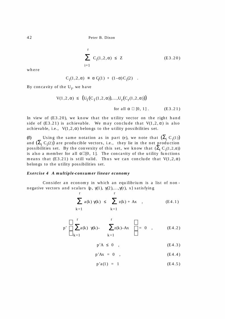
Exercise 4 A multiple-consumer linear economy
Consider an economy in which an equilibrium is a list of non -negative vectors and scalars {p, γ(1), γ(2),...,γ(r), x} satisfying
Σk=1
r
a(k) γ(k) ≤ Σk=1
r
z(k) + Ax , (E4.1)
p′
Σ
k=1
r
a(k) γ(k)– Σk=1
r
z(k)–Ax = 0 , (E4.2)
p′A ≤ 0 , (E4.3)
p′Ax = 0 , (E4.4)
p′a(1) = 1 (E4.5)
The Mathematical Programming Approach to Applied General Equilibrium 43
and
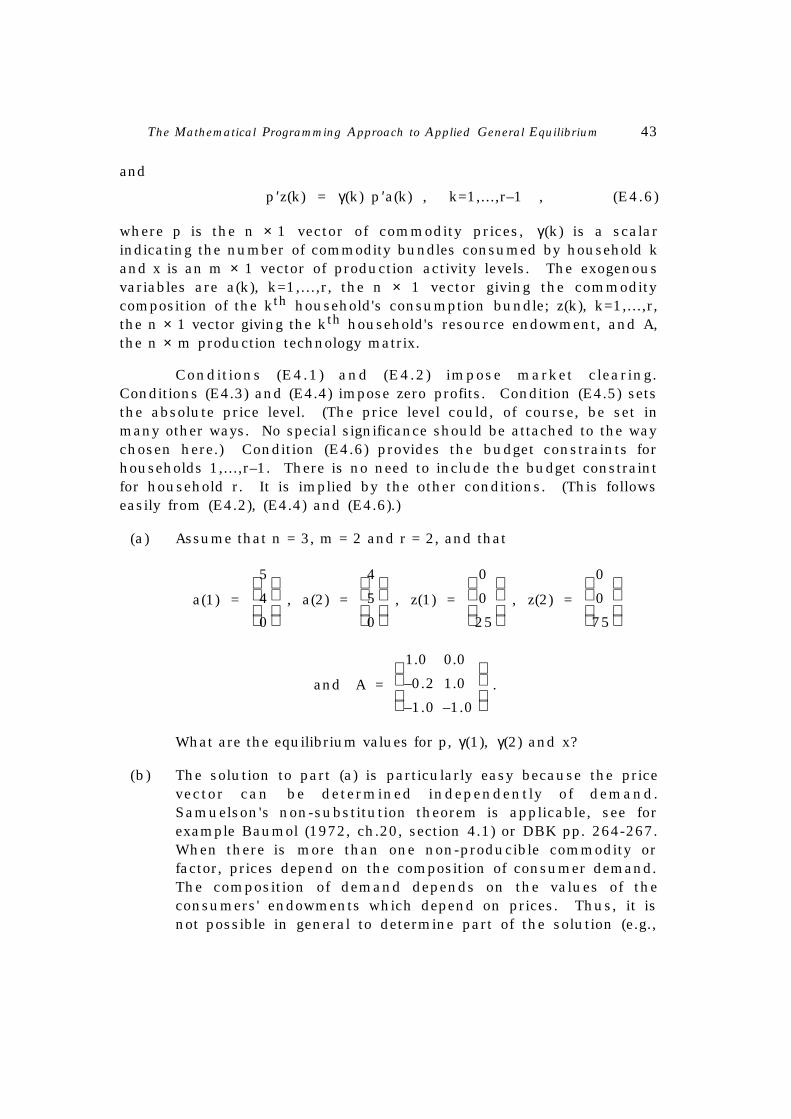
p′z(k) = γ(k) p ′a(k) , k=1,...,r–1 , (E4.6)
where p is the n × 1 vector of commodity prices, γ(k) is a scalarindicating the number of commodity bundles consumed by household kand x is an m × 1 vector of production activity levels. The exogenousvariables are a(k), k=1,...,r, the n × 1 vector giving the commoditycomposition of the kth household's consumption bundle; z(k), k=1,...,r,the n × 1 vector giving the kth household's resource endowment, and A,the n × m production technology matrix.
Conditions (E4.1) and (E4.2) impose market clearing.Conditions (E4.3) and (E4.4) impose zero profits. Condition (E4.5) setsthe absolute price level. (The price level could, of course, be set inmany other ways. No special significance should be attached to the waychosen here.) Condition (E4.6) provides the budget constraints forhouseholds 1,...,r–1. There is no need to include the budget constraintfor household r. It is implied by the other conditions. (This followseasily from (E4.2), (E4.4) and (E4.6).)
(a) Assume that n = 3, m = 2 and r = 2, and that
a(1) =
5
4
0
, a(2) =
4
5
0
, z(1) =
0
0
25
, z(2) =
0
0
75
and A =
1.0 0.0
–0.2 1.0
–1.0 –1.0
.
What are the equilibrium values for p, γ(1), γ(2) and x?
(b) The solution to part (a) is particularly easy because the pricevector can be determined independently of demand.Samuelson's non-substitution theorem is applicable, see forexample Baumol (1972, ch.20, section 4.1) or DBK pp. 264-267.When there is more than one non-producible commodity orfactor, prices depend on the composition of consumer demand.The composition of demand depends on the values of theconsumers' endowments which depend on prices. Thus, it isnot possible in general to determine part of the solution (e.g.,
44 Peter B. Dixon
the prices) of model (E4.1) – (E4.6) independently of the rest ofthe solution. Suggest how (E4.1) – (E4.6) might be solved by asequence of linear programs.
Answer to Exercise 4
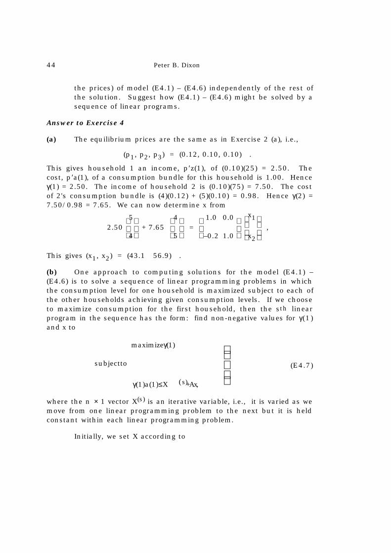
(a) The equilibrium prices are the same as in Exercise 2 (a), i.e.,
(p1, p2, p3) = (0.12, 0.10, 0.10) .
This gives household 1 an income, p′z(1), of (0.10)(25) = 2.50. Thecost, p ′a(1), of a consumption bundle for this household is 1.00. Henceγ(1) = 2.50. The income of household 2 is (0.10)(75) = 7.50. The costof 2's consumption bundle is (4)(0.12) + (5)(0.10) = 0.98. Hence γ(2) =7.50/0.98 = 7.65. We can now determine x from
2.50
5
4 + 7.65
4
5 =
1.0 0.0
–0.2 1.0
x1
x2
,
This gives (x1, x2) = (43.1 56.9) .
(b) One approach to computing solutions for the model (E4.1) –(E4.6) is to solve a sequence of linear programming problems in whichthe consumption level for one household is maximized subject to each ofthe other households achieving given consumption levels. If we chooseto maximize consumption for the first household, then the sth linearprogram in the sequence has the form: find non-negative values for γ(1)and x to
maximizeγ(1)
subjectto
γ(1)a(1)≤X ( s)+Ax,
(E4.7)
where the n × 1 vector X(s) is an iterative variable, i.e., it is varied as wemove from one linear programming problem to the next but it is heldconstant within each linear programming problem.
Initially, we set X according to
The Mathematical Programming Approach to Applied General Equilibrium 45
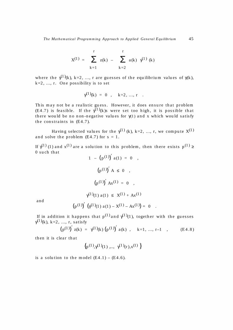
X(1) = Σk=1
r
z(k) – Σk=2
r
a(k) γ(1) (k)
where the γ(1)(k), k=2, ..., r are guesses of the equilibrium values of γ(k),k=2, ..., r. One possibility is to set
γ(1)(k) = 0 , k=2, ..., r .
This may not be a realistic guess. However, it does ensure that problem(E4.7) is feasible. If the γ(1)(k)s were set too high, it is possible thatthere would be no non-negative values for γ(1) and x which would satisfythe constraints in (E4.7).
Having selected values for the γ(1) (k), k=2, ..., r, we compute X(1)
and solve the problem (E4.7) for s = 1.
If γ(1) (1) and x(1) are a solution to this problem, then there exists p(1) ≥0 such that
1 – (p(1))′ a(1) = 0 ,
(p(1))′ A ≤ 0 ,
(p(1))′ Ax(1) = 0 ,
γ(1)(1) a(1) ≤ X(1) + Ax(1)
and (p(1))′ (γ(1)(1) a(1) – X(1) – Ax(1)) = 0 .
If in addition it happens that p(1) and γ(1)(1), together with the guesses
γ(1)(k), k=2, ..., r, satisfy
(p(1))′ z(k) = γ(1)(k) (p(1))′ a(k) , k=1, ..., r–1 , (E4.8)
then it is clear that
{ }p(1),γ(1)(1) ,..., γ(1)(r),x(1)
is a solution to the model (E4.1) – (E4.6).

46 Peter B. Dixon
Normally, we will not be so lucky that (E4.8) is satisfied. Weproceed by updating our guesses for γ(k), k=2, ..., r, recomputing X andre-solving (E4.7). An updating formula which is often satisfactory is
γ(s)(k) = (p(s–1))′ z(k) / (p(s–1))′ a(k) , k=2, ..., r, (E4.9)
i.e., our guess for γ(k), k=2, ..., r, to be used in the sth linear programis obtained by calculating the number of consumption bundles whichconsumer k could afford at the commodity prices, p(s–1), revealed fromthe solution to our (s–1)th linear program.
When (E4.9) gives
γs(k) = γs–1(k) , k=2, ..., r ,
then convergence has occurred and we have found a solution to themodel (E4.1) – (E4.6). Convergence cannot be guaranteed. In practice,however, convergence is usually achieved with a small value for s (e.g., s= 3). The reason is that the value for p emerging from (E4.7) isnormally fairly insensitive to variations in X. If there is only one non-producible commodity, (the Samuelson non-substitution situation) thenp is completely insensitive to variations in X. In this case, the search foran equilibrium for the model (E4.1) – (E4.6) will necessitate thesolution of no more than two linear programming problems of the form(E4.7).
Exercise 5 A linear economy with a utility maximizing consumer
Consider an economy in which an equilibrium is a list of non-negative vectors and scalars {p, c, Y, x} satisfying:
cmaximizesU(c)
subjectto
p′c=Y
(E5.1)
c≤z+Ax ,
p′(c–z–Ax)=0,(E5.2)
p′A≤0 ,
p′Ax=0(E5.3)

The Mathematical Programming Approach to Applied General Equilibrium 47
andp′z = 1 , (E5.4)
where p is the n × 1 vector of commodity prices, c is the n × 1 vector ofhousehold consumption by commodity, the scalar Y is householdexpenditure and x is the m × 1 vector of production activity levels. Theexogenous variables are z, the n × 1 vector giving the economy'sresource endowments and A, the n × m production technology matrix.U is a utility function describing household preferences.
Condition (E5.1) says that the consumption vector, c, is chosento maximize utility subject to the household budget constraint.Conditions (E5.2) and (E5.3) are familiar from earlier exercises.Condition (E5.4) sets the absolute price level.15
(a) For (p, c, Y, x) satisfying (E5.1) – (E5.4), show that
Y = p ′z . (E5.5)
(b) Assume that
U(c) = maxγ
{γ aγ ≤ c} (E5.6)
where a is a non-negative n × 1 vector. Assume in addition thatn = 3 and
a =
5
4
0
. (E5.7)
Evaluate
U
5
4
0
, U
6
4
0
, U
5
5
5
, U
5
5
0
.
15 In previous exercises we fixed the absolute value of a consumption bundle,see (E2.3). Here, where the composition of the consumption bundle ispotentially endogenous, it is convenient to fix, instead, the absolute value ofthe resource endowment.

48 Peter B. Dixon
Sketch some indifference curves for the utility function (E5.6) –(E5.7) in commodity 1/commodity 2 space. Solve the model(E5.1) – (E5.4) assuming that
z =
0
0
100
, A =
1.0 0.0
–0.2 1.0
–1.0 –1.0
, (E5.8)
and that U(c) is given by (E5.6) – (E5.7).
(c ) Assume that
U(c) = maxγ
{1′h γ aγ ≤ c, γ >_ 0} for c >_ 0 , (E5.9)
where a is now a non-negative n × h matrix and γ is an h × 1vector. 1′
h is a 1 × h vector of ones. Assume in addition that n =3, h = 2 and that
a =
3 2
2 3
0 0
. (E5.10)
Evaluate
U
30
20
0
, U
20
30
0
, U
25
25
0
, U
40
20
0
, U
20
40
0
.
Sketch some indifference curves for utility function (E5.9) –(E5.10) in commodity 1/commodity 2 space. Solve the model(E5.1) – (E5.4) assuming that z and A are given by (E5.8) andthat U(c) is given by (E5.9) – (E5.10).
(d ) Write a linear programming problem which would be a suitablevehicle for solving the model (E5.1) – (E5.4) where the utilityfunction takes the form (E5.9).
(e ) In a utility maximizing model with the utility specification(E5.9), the expenditure elasticities of demand for all goods areunity. A specification which allows expenditure elasticities tovary from unity but is still convenient for use in a linearprogramming framework is
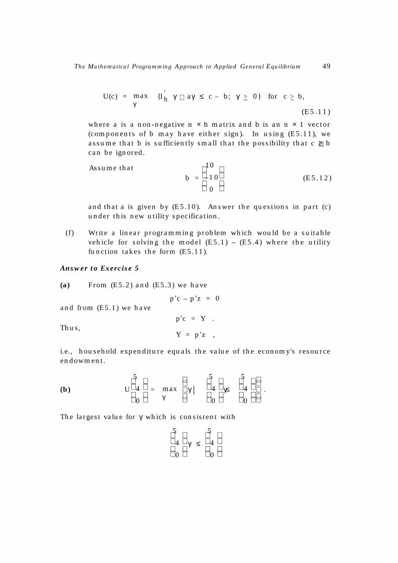
The Mathematical Programming Approach to Applied General Equilibrium 49
U(c) = maxγ
{1′h γ aγ ≤ c – b; γ >_ 0} for c >_ b,
(E5.11)
where a is a non-negative n × h matrix and b is an n × 1 vector(components of b may have either sign). In using (E5.11), weassume that b is sufficiently small that the possibility that c ≥ bcan be ignored.
Assume thatb =
10
–10
0
(E5.12)
and that a is given by (E5.10). Answer the questions in part (c)under this new utility specification.
(f) Write a linear programming problem which would be a suitablevehicle for solving the model (E5.1) – (E5.4) where the utilityfunction takes the form (E5.11).
Answer to Exercise 5
(a) From (E5.2) and (E5.3) we have
p′c – p ′z = 0and from (E5.1) we have
p′c = Y .Thus,
Y = p ′z ,
i.e., household expenditure equals the value of the economy's resourceendowment.
(b) U
5
4
0
= maxγ
γ|
5
4
0
γ≤
5
4
0
.
The largest value for γ which is consistent with
5
4
0
γ ≤
5
4
0
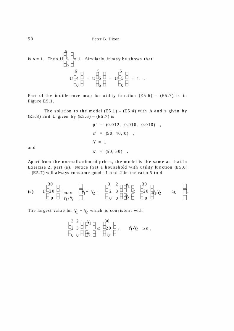
50 Peter B. Dixon
is γ = 1. Thus U
5
4
0
= 1. Similarly, it may be shown that
U
6
4
0
= U
5
5
5
= U
5
5
0
= 1 .
Part of the indifference map for utility function (E5.6) – (E5.7) is inFigure E5.1.
The solution to the model (E5.1) – (E5.4) with A and z given by(E5.8) and U given by (E5.6) – (E5.7) is
p′ = (0.012, 0.010, 0.010) ,
c′ = (50, 40, 0) ,
Y = 1and
x′ = (50, 50) .
Apart from the normalization of prices, the model is the same as that inExercise 2, part (a). Notice that a household with utility function (E5.6)– (E5.7) will always consume goods 1 and 2 in the ratio 5 to 4.
(c) U
30
20
0
= maxγ1,γ2
γ1+ γ2|
3 2
2 3
0 0
γ1
γ2≤
30
20
0
;γ1,γ2 ≥0 .
The largest value for γ1 + γ2 which is consistent with
3 2
2 3
0 0
γ1
γ2 ≤
30
20
0
; γ1,γ2 ≥ 0 ,
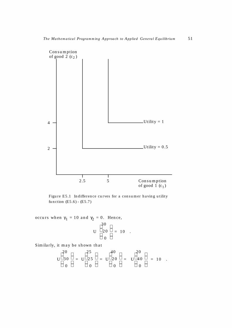
The Mathematical Programming Approach to Applied General Equilibrium 51
Utility = 1
Utility = 0.5
2.5 5 Consumptionof good 1 (c1)
2
4
Consumptionof good 2 (c2 )
Figure E5.1 Indifference curves for a consumer having utilityfunction (E5.6) - (E5.7)
occurs when γ1 = 10 and γ2 = 0. Hence,
U
30
20
0
= 10 .
Similarly, it may be shown that
U
20
30
0
= U
25
25
0
= U
40
20
0
= U
20
40
0
= 10 .
52 Peter B. Dixon
Part of the indifference map for utility function (E5.9) – (E5.10) is inFigure E5.2.
With only one non-producible good, a change in the utilityfunction does not affect the equilibrium prices in the model (E5.1) –(E5.4). Thus, as in part (a), we have
p′ = (0.012, 0.010, 0.010)and
Y = 1 . (E5.13)
The household budget constraint is
0.012c1 + 0.010c2 + 0.010c3 = 1 . (E5.14)
Under (E5.9) – (E5.10), consumption of good 3 does not contribute toutility. Thus c3 = 0 and (E5.14) may be reduced to
0.012c1 + 0.010c2 = 1 . (E5.15)
By representing (E5.15) in Figure E5.2 we find that the utilitymaximizing consumption vector consistent with the budget constraint is
c′ = (37.0, 55.6, 0) .
Finally, we compute the activity levels, x, from
37.0
55.6 =
0
0 +
1.0 0.0
–0.2 1.0
x1
x2 , (E5.16)
giving
x′ = (37.0, 63.0) .
In (E5.16), the market clearing equation for commodity 3 has beenomitted. On the other hand, in (E5.13) we have used (E5.5). With thevalue of consumption equal to the value of resources, demand equal tosupply for goods 1 and 2, zero pure profits in all production activities,and p3 > 0, it is easy to show that demand must equal supply forcommodity 3.
(d) Consider the problem of choosing non-negative values for γ and xto

The Mathematical Programming Approach to Applied General Equilibrium 53
100
6055.6
40
20
0
30
20 6030 83.337
Consumptionof good 1
Budget Line
Utility = 10
Utility = 18.53
Utility = 20
Consumptionof good 2
B
A
I
II
Figure E5.2 Indifference map and budget line for theconsumer in model (E5.1) - (E5.4), assuming (E5.8) - (E5.10)
Indifference curves may be constructed by using the two rays0A and 0B. With the consumption bundle at point I on ray 0A,we have utility of 10(γ1 = 10, γ2 = 0). At point II on ray 0B,utility is also 10(γ1 = 0, γ2 = 10). Points on the straight linebetween I and II give utility of 10 with both consumptionactivities being used. For example, the point half waybetween I and II (i.e., c1 = 25, c2 = 25) gives utility of 10 with γ1 =5 and γ2 = 5.
54 Peter B. Dixon
maximize 1′h γ (E5.17)
subject toaγ ≤ z + Ax . (E5.18)
The non-negative vectors γ_ and x
_ are a solution to this problem if and
only if there exists p_ >_ 0, such that
1′h – p
_′a ≤ 0 , (E5.19)
(1′h – p
_′a)γ
_ = 0 , (E5.20)
p_
′A ≤ 0 , (E5.21)
p_
′A x_ = 0 , (E5.22)
aγ_ – z – Ax
_ ≤ 0 (E5.23)
and
p_
′(aγ_ – z – Ax
_) = 0 . (E5.24)
Now we show that
p =
1
p_
′z
p
_ , (E5.25)16
c = aγ_ , (E5.26)
Y =
1
p_
′z
p_ ′aγ
_ , (E5.27)
and
x = x_ (E5.28)
is a solution to the model (E5.1) – (E5.4) where the utility function hasthe form (E5.9). When we have done this, we will have established thatthe model can be solved by first finding the primal and dual solutions tothe linear programming problem (E5.17) – (E5.18) and then usingformulae (E5.25) – (E5.28).
16 In writing (E5.25), we assume that p_´z > 0.

The Mathematical Programming Approach to Applied General Equilibrium 55
Clearly our suggested solution (E5.25) – (E5.28) satisfiesconditions (E5.2) – (E5.4). Does it satisfy (E5.1)? Under (E5.9), thesolution for the consumer problem (E5.1) is the solution for c in theproblem of choosing non-negative values for c and γ to
maximize 1′h γ (E5.29)
subject to aγ ≤ c (E5.30)
and p′c ≤ Y . (E5.31)
Non-negative vectors γ and c are a solution of this problem if and only ifthere exist q >_ 0 and λ >_ 0 such that
1′
h–q ′a≤0,
(1′h–q ′a)γ=0,
(E5.32)
}q′– λp′≤0,(q ′–λp ′)c=0 , (E5.33)
}aγ–c≤0,q′(aγ–c)=0, (E5.34)
p ′c–Y≤0
and
λ(p ′c–Y)=0.
(E5.35)
If p and Y are given by (E5.25) and (E5.27), then it is apparent that c =aγ_ and γ = γ
_ is a solution to (E5.29) – (E5.31). (Conditions (E5.32) –
(E5.35) are satisfied with λ = p_
′z and q = p_.) We may conclude that our
suggested solution (E5.25) – (E5.28) for the model (E5.1) – (E5.4) isconsistent with the utility maximizing condition (E5.1) where the utilityfunction is of the form (E5.9).

56 Peter B. Dixon
(e)
U
30
20
0
= maxγ1,γ2
γ1+ γ2
3 2
2 3
0 0
γ1
γ2≤
30
20
0
–
10
–10
0
;γ 1,γ2 >_ 0
(E5.36)
Figure E5.3 shows that the solution to the problem on the right hand
side of (E5.36) is γ1 = 0, γ2 = 10. Hence U
30
20
0
= 10. Similarly, it may
be shown that
U
20
30
0
= 5 , U
25
25
0
= 712 , U
40
20
0
= 12 and U
20
40
0
= 5 .
Part of the indifference map for the utility function (E5.11) withparameter values given by (E5.10) and (E5.12) is in Figure E5.4.
With A and z given by (E5.8), the equilibrium prices andexpenditure level continue to be as in parts (b) and (c), that is
p′ = (0.012, 0.010, 0.010)and
Y = 1 .
The household budget constraint is still given by (E5.14) whichreduces to (E5.15) when it is recognized that good 3 is not consumed.By drawing the budget constraint in Figure E5.4, we find that
c′ = (46.3, 44.4, 0) .
Finally we compute the activity levels, x, from
46.3
44.4 =
1.0 0.0
–0.2 1.0
x1
x2
,
giving
x′ = (46.3, 53.7) .
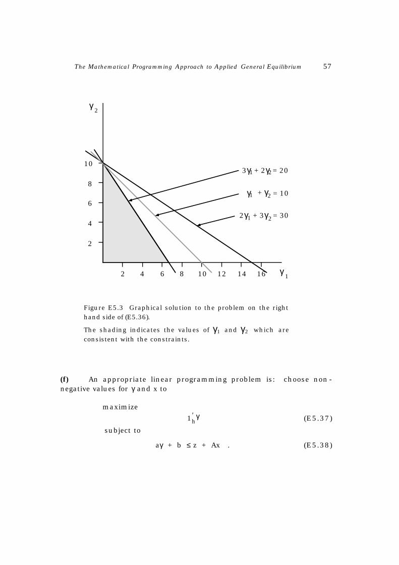
The Mathematical Programming Approach to Applied General Equilibrium 57
= 302γ 1 + 3γ 2
2γ
12 4 6 8 10 12 14 16 γ
2
4
6
8
10 = 203γ 1+ 2γ 2
= 10γ 1 + γ 2
Figure E5.3 Graphical solution to the problem on the righthand side of (E5.36).
The shading indicates the values of γ1 and γ2 which areconsistent with the constraints.
(f) An appropriate linear programming problem is: choose non -negative values for γ and x to
maximize
1′h
γ (E5.37)
subject to
aγ + b ≤ z + Ax . (E5.38)

58 Peter B. Dixon
Where γ_, x
_ and p
_ are a primal and associated dual solution to this
problem, it can be shown, by following the method in part (d), that
p =
1
p_
′z
p_ ,
c = aγ_ + b ,
Y =
1
p_
′z
(p_
′aγ_+p
_′b) ,
and
x = x_
is a solution to the model (E5.1) – (E5.4) when the utility function hasthe form (E5.11).
Exercise 6 A linear economy with several utility maximizingconsumers
Consider an economy in which an equilibrium is a list of non -negative vectors and scalars
{p, c(1), c(2), ..., c(r), Y(1), ..., Y(r), x} satisfying the following conditions:
foreachk ,k=1,... ,r ,c(k)maximizes
U k(c(k))subjecttop ′c(k)=Y(k), (E6.1)
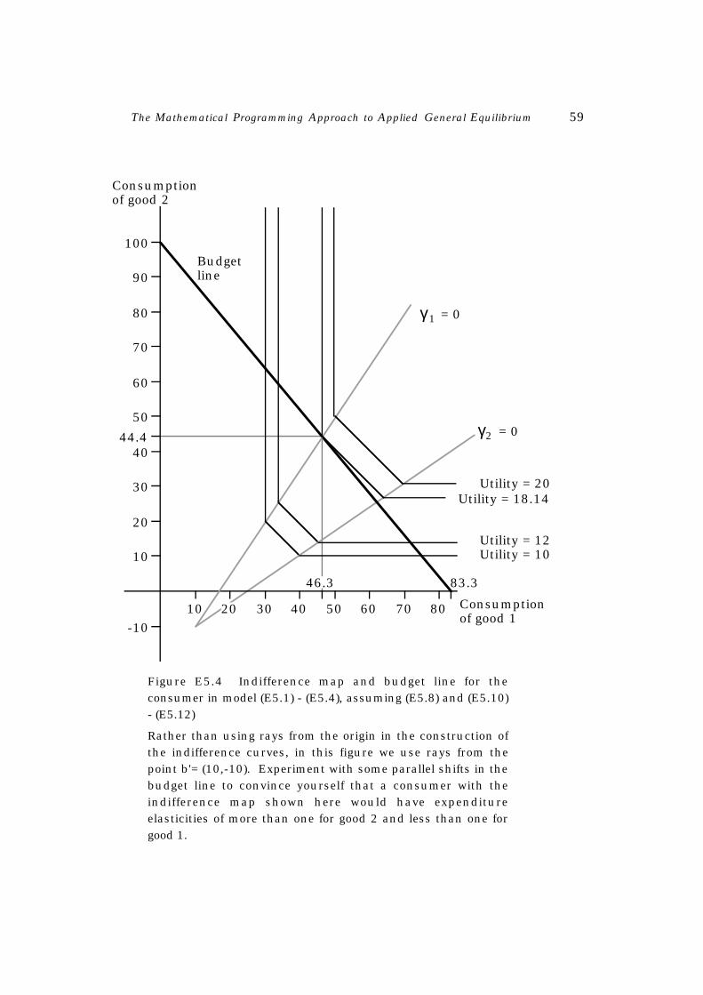
The Mathematical Programming Approach to Applied General Equilibrium 59
44.4
100
-10
10
20
30
40
50
60
70
80
90
10 20 30 60 70
83.346.3
40 50 80
Consumptionof good 2
Consumptionof good 1
Utility = 10
Utility = 18.14
Utility = 12
Utility = 20
γ = 0 1
γ = 0 2
Budgetline
Figure E5.4 Indifference map and budget line for theconsumer in model (E5.1) - (E5.4), assuming (E5.8) and (E5.10)- (E5.12)
Rather than using rays from the origin in the construction ofthe indifference curves, in this figure we use rays from thepoint b'= (10,-10). Experiment with some parallel shifts in thebudget line to convince yourself that a consumer with theindifference map shown here would have expenditureelasticities of more than one for good 2 and less than one forgood 1.
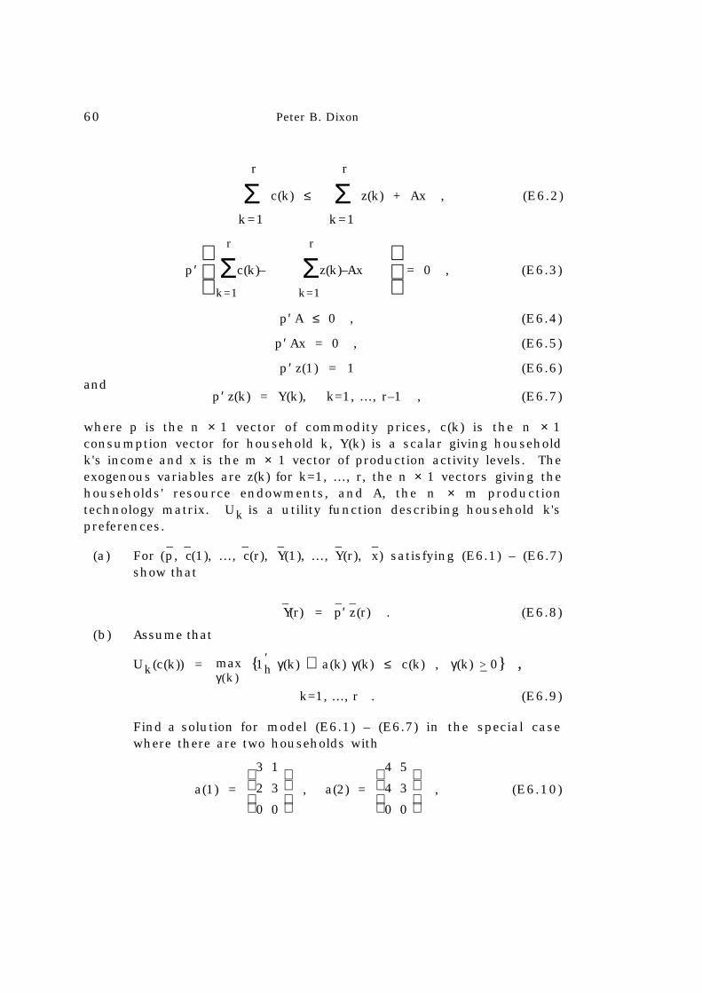
60 Peter B. Dixon
Σk=1
r
c(k) ≤ Σk=1
r
z(k) + Ax , (E6.2)
p′
Σ
k=1
r
c(k)– Σk=1
r
z(k)–Ax = 0 , (E6.3)
p′ A ≤ 0 , (E6.4)
p′ Ax = 0 , (E6.5)
p′ z(1) = 1 (E6.6)and
p′ z(k) = Y(k), k=1, ..., r–1 , (E6.7)
where p is the n × 1 vector of commodity prices, c(k) is the n × 1consumption vector for household k, Y(k) is a scalar giving householdk's income and x is the m × 1 vector of production activity levels. Theexogenous variables are z(k) for k=1, ..., r, the n × 1 vectors giving thehouseholds' resource endowments, and A, the n × m productiontechnology matrix. Uk is a utility function describing household k'spreferences.
(a) For (p_, c
_(1), ..., c
_(r), Y
_(1), ..., Y
_(r), x
_) satisfying (E6.1) – (E6.7)
show that
Y_(r) = p
_′ z_(r) . (E6.8)
(b) Assume that
Uk(c(k)) = maxγ(k)
{1′h γ(k) a(k) γ(k) ≤ c(k) , γ(k) >_ 0} ,
k=1, ..., r . (E6.9)
Find a solution for model (E6.1) – (E6.7) in the special casewhere there are two households with
a(1) =
3 1
2 3
0 0
, a(2) =
4 5
4 3
0 0
, (E6.10)
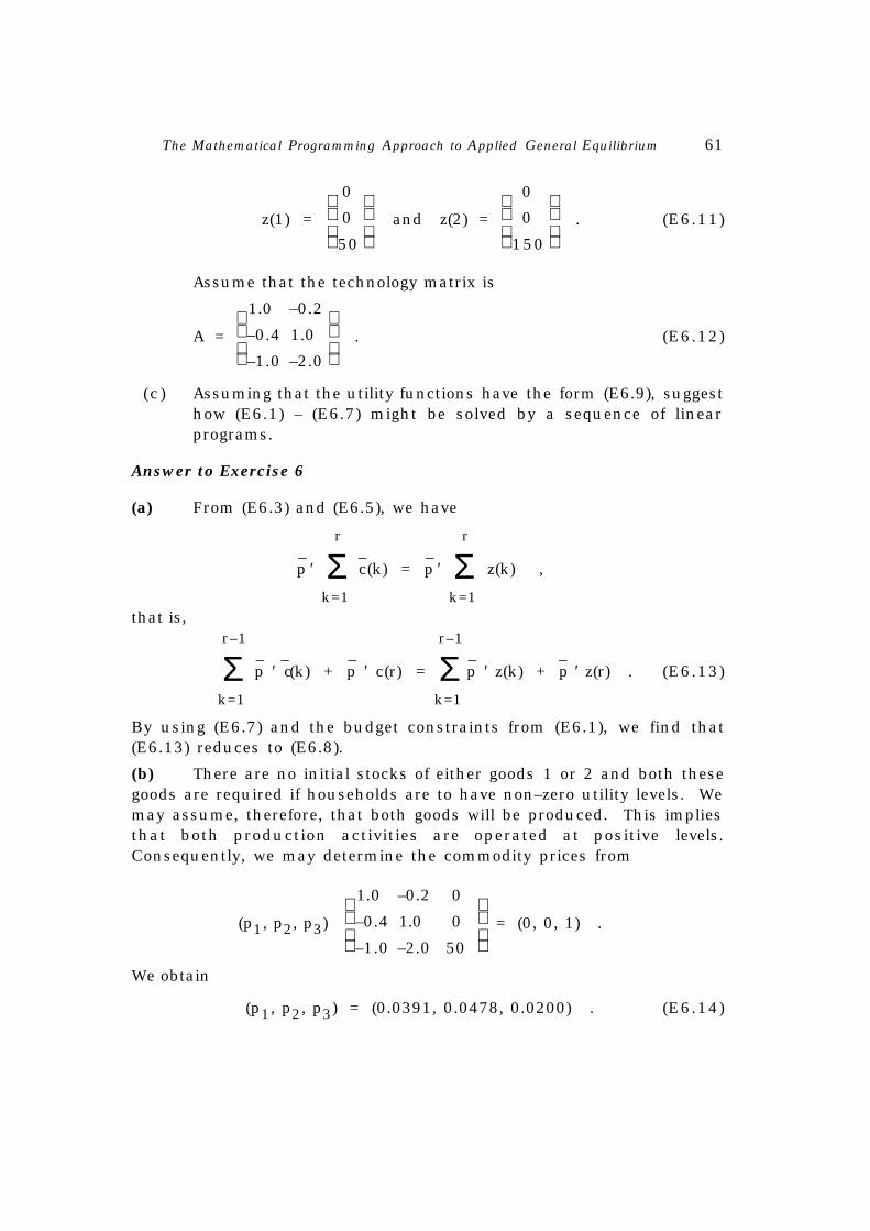
The Mathematical Programming Approach to Applied General Equilibrium 61
z(1) =
0
0
50
and z(2) =
0
0
150
. (E6.11)
Assume that the technology matrix is
A =
1.0 –0.2
–0.4 1.0
–1.0 –2.0
. (E6.12)
(c ) Assuming that the utility functions have the form (E6.9), suggesthow (E6.1) – (E6.7) might be solved by a sequence of linearprograms.
Answer to Exercise 6
(a) From (E6.3) and (E6.5), we have
p_
′ Σk=1
r
c_(k) = p
_ ′ Σ
k=1
r
z(k) ,
that is,
Σk=1
r–1
p_ ′ c
_(k) + p
_ ′ c(r) = Σ
k=1
r–1
p_ ′ z(k) + p
_ ′ z(r) . (E6.13)
By using (E6.7) and the budget constraints from (E6.1), we find that(E6.13) reduces to (E6.8).
(b) There are no initial stocks of either goods 1 or 2 and both thesegoods are required if households are to have non–zero utility levels. Wemay assume, therefore, that both goods will be produced. This impliesthat both production activities are operated at positive levels.Consequently, we may determine the commodity prices from
(p1, p2, p3)
1.0 –0.2 0
–0.4 1.0 0
–1.0 –2.0 50
= (0, 0, 1) .
We obtain
(p1, p2, p3) = (0.0391, 0.0478, 0.0200) . (E6.14)
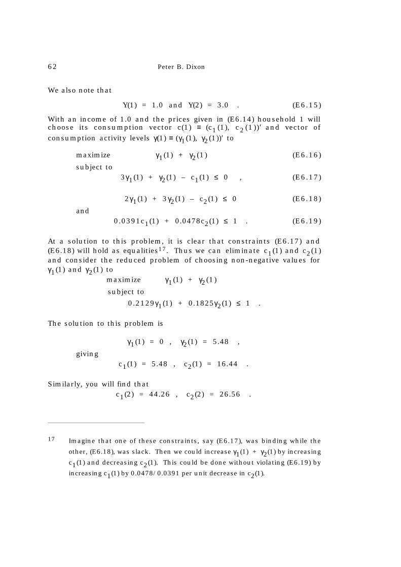
62 Peter B. Dixon
We also note that
Y(1) = 1.0 and Y(2) = 3.0 . (E6.15)
With an income of 1.0 and the prices given in (E6.14) household 1 willchoose its consumption vector c(1) ≡ (c1 (1), c2 (1)) ′ and vector of
consumption activity levels γ(1) ≡ (γ1(1), γ2(1))′ to
maximize γ1(1) + γ2(1) (E6.16)
subject to3γ1(1) + γ2(1) – c1(1) ≤ 0 , (E6.17)
2γ1(1) + 3γ2(1) – c2(1) ≤ 0 (E6.18)
and0.0391c1(1) + 0.0478c2(1) ≤ 1 . (E6.19)
At a solution to this problem, it is clear that constraints (E6.17) and(E6.18) will hold as equalities17. Thus we can eliminate c1(1) and c2(1)and consider the reduced problem of choosing non-negative values forγ1(1) and γ2(1) to
maximize γ1(1) + γ2(1)
subject to
0.2129γ1(1) + 0.1825γ2(1) ≤ 1 .
The solution to this problem is
γ1(1) = 0 , γ2(1) = 5.48 ,
givingc1(1) = 5.48 , c2(1) = 16.44 .
Similarly, you will find thatc1(2) = 44.26 , c2(2) = 26.56 .
17 Imagine that one of these constraints, say (E6.17), was binding while the
other, (E6.18), was slack. Then we could increase γ1(1) + γ2(1) by increasing
c1(1) and decreasing c2(1). This could be done without violating (E6.19) by
increasing c1(1) by 0.0478/0.0391 per unit decrease in c2(1).
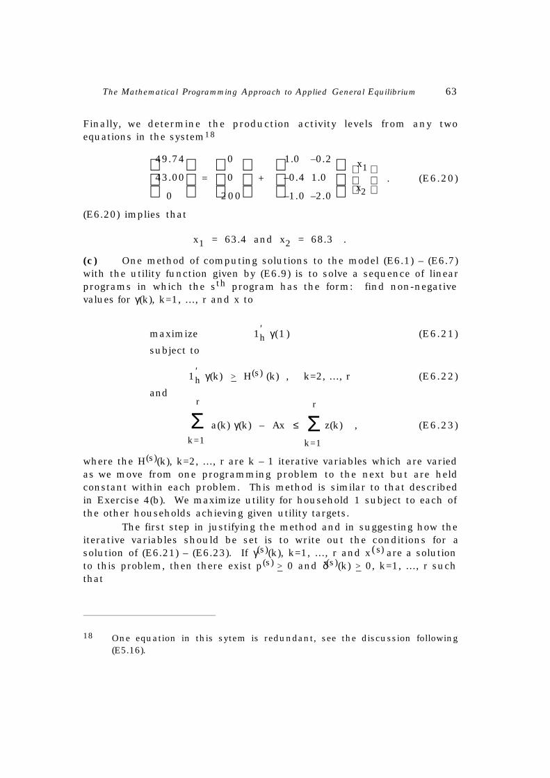
The Mathematical Programming Approach to Applied General Equilibrium 63
Finally, we determine the production activity levels from any twoequations in the system18
49.74
43.00
0
=
0
0
200
+
1.0 –0.2
–0.4 1.0
–1.0 –2.0
x1
x2 . (E6.20)
(E6.20) implies that
x1 = 63.4 and x2 = 68.3 .
(c) One method of computing solutions to the model (E6.1) – (E6.7)with the utility function given by (E6.9) is to solve a sequence of linearprograms in which the sth program has the form: find non-negativevalues for γ(k), k=1, ..., r and x to
maximize 1′h γ(1) (E6.21)
subject to
1′h γ(k) >_ H(s) (k) , k=2, ..., r (E6.22)
and
Σk=1
r
a(k) γ(k) – Ax ≤ Σk=1
r
z(k) , (E6.23)
where the H(s)(k), k=2, ..., r are k – 1 iterative variables which are variedas we move from one programming problem to the next but are heldconstant within each problem. This method is similar to that describedin Exercise 4(b). We maximize utility for household 1 subject to each ofthe other households achieving given utility targets.
The first step in justifying the method and in suggesting how theiterative variables should be set is to write out the conditions for asolution of (E6.21) – (E6.23). If γ(s)(k), k=1, ..., r and x( s) are a solutionto this problem, then there exist p(s) >_ 0 and δ(s)(k) >_ 0, k=1, ..., r suchthat
18 One equation in this sytem is redundant, see the discussion following(E5.16).
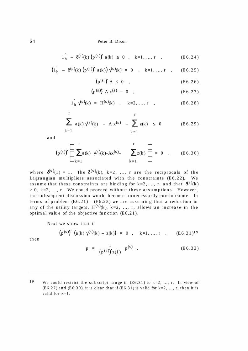
64 Peter B. Dixon
1′h – δ(s)(k) (p(s))′ a(k) ≤ 0 , k=1, ..., r , (E6.24)
(1′h – δ(s)(k) (p(s))′ a(k)) γ(s)(k) = 0 , k=1, ..., r , (E6.25)
(p(s))′ A ≤ 0 , (E6.26)
(p(s))′ A x(s) = 0 , (E6.27)
1′h γ(s)(k) = H(s)(k) , k=2, ..., r , (E6.28)
Σk=1
r
a(k) γ(s)(k) – A x(s) – Σk=1
r
z(k) ≤ 0 (E6.29)
and
(p(s))′
Σ
k=1
r
a(k) γ(s)(k)–Ax(s)– Σk=1
r
z(k) = 0 , (E6.30)
where δ(s)(1) = 1. The δ (s)(k), k=2, ..., r are the reciprocals of theLagrangian multipliers associated with the constraints (E6.22). Weassume that these constraints are binding for k=2, ..., r, and that δ(s)(k)> 0, k=2, ..., r. We could proceed without these assumptions. However,the subsequent discussion would become unnecessarily cumbersome. Interms of problem (E6.21) – (E6.23) we are assuming that a reduction inany of the utility targets, H(s)(k), k=2, ..., r, allows an increase in theoptimal value of the objective function (E6.21).
Next we show that if
(p(s))′ (a(k) γ(s)(k) – z(k)) = 0 , k=1, ..., r , (E6.31)19
then
p = 1
(p(s))′z(1) p(s) , (E6.32)
19 We could restrict the subscript range in (E6.31) to k=2, ..., r. In view of(E6.27) and (E6.30), it is clear that if (E6.31) is valid for k=2, ..., r, then it isvalid for k=1.
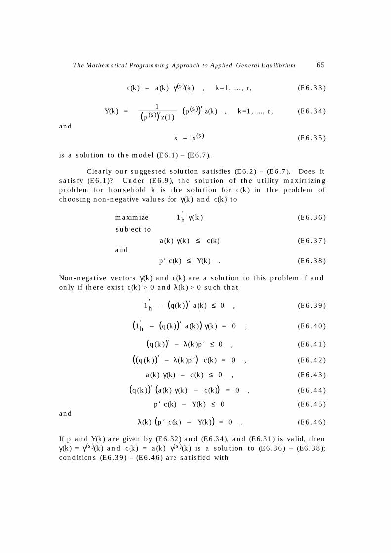
The Mathematical Programming Approach to Applied General Equilibrium 65
c(k) = a(k) γ(s)(k) , k=1, ..., r, (E6.33)
Y(k) = 1
(p(s))′z(1) (p(s))′ z(k) , k=1, ..., r, (E6.34)
and
x = x(s) (E6.35)
is a solution to the model (E6.1) – (E6.7).
Clearly our suggested solution satisfies (E6.2) – (E6.7). Does itsatisfy (E6.1)? Under (E6.9), the solution of the utility maximizingproblem for household k is the solution for c(k) in the problem ofchoosing non-negative values for γ(k) and c(k) to
maximize 1′h γ(k) (E6.36)
subject to
a(k) γ(k) ≤ c(k) (E6.37)and
p′ c(k) ≤ Y(k) . (E6.38)
Non-negative vectors γ(k) and c(k) are a solution to this problem if andonly if there exist q(k) >_ 0 and λ(k) >_ 0 such that
1′h – (q(k)) ′ a(k) ≤ 0 , (E6.39)
(1′h – (q(k)) ′ a(k)) γ(k) = 0 , (E6.40)
(q(k))′ – λ(k)p ′ ≤ 0 , (E6.41)
((q(k))′ – λ(k)p ′) c(k) = 0 , (E6.42)
a(k) γ(k) – c(k) ≤ 0 , (E6.43)
(q(k))′ (a(k) γ(k) – c(k)) = 0 , (E6.44)
p′ c(k) – Y(k) ≤ 0 (E6.45)and
λ(k) (p ′ c(k) – Y(k)) = 0 . (E6.46)
If p and Y(k) are given by (E6.32) and (E6.34), and (E6.31) is valid, thenγ(k) = γ(s)(k) and c(k) = a(k) γ(s)(k) is a solution to (E6.36) – (E6.38);conditions (E6.39) – (E6.46) are satisfied with
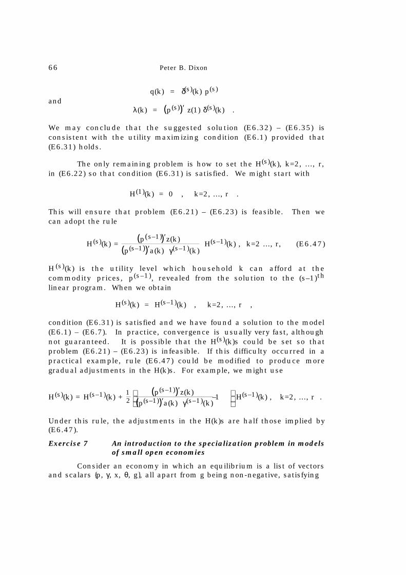
66 Peter B. Dixon
q(k) = δ(s)(k) p(s)
andλ(k) = (p(s))′ z(1) δ(s)(k) .
We may conclude that the suggested solution (E6.32) – (E6.35) isconsistent with the utility maximizing condition (E6.1) provided that(E6.31) holds.
The only remaining problem is how to set the H(s)(k), k=2, ..., r,in (E6.22) so that condition (E6.31) is satisfied. We might start with
H(1)(k) = 0 , k=2, ..., r .
This will ensure that problem (E6.21) – (E6.23) is feasible. Then wecan adopt the rule
H(s)(k) = (p(s–1))′z(k)
(p(s–1))′a(k) γ(s–1)(k) H(s–1)(k) , k=2 ..., r, (E6.47)
H (s)(k) is the utility level which household k can afford at thecommodity prices, p(s–1), revealed from the solution to the (s–1)th
linear program. When we obtain
H(s)(k) = H(s–1)(k) , k=2, ..., r ,
condition (E6.31) is satisfied and we have found a solution to the model(E6.1) – (E6.7). In practice, convergence is usually very fast, althoughnot guaranteed. It is possible that the H(s)(k)s could be set so thatproblem (E6.21) – (E6.23) is infeasible. If this difficulty occurred in apractical example, rule (E6.47) could be modified to produce moregradual adjustments in the H(k)s. For example, we might use
H(s)(k) = H(s–1)(k) + 12
(p(s–1))′z(k)
(p(s–1))′a(k) γ(s–1)(k)–1 H(s–1)(k) , k=2, ..., r .
Under this rule, the adjustments in the H(k)s are half those implied by(E6.47).
Exercise 7 An introduction to the specialization problem in modelsof small open economies
Consider an economy in which an equilibrium is a list of vectorsand scalars {p, γ, x, θ, g}, all apart from g being non-negative, satisfying
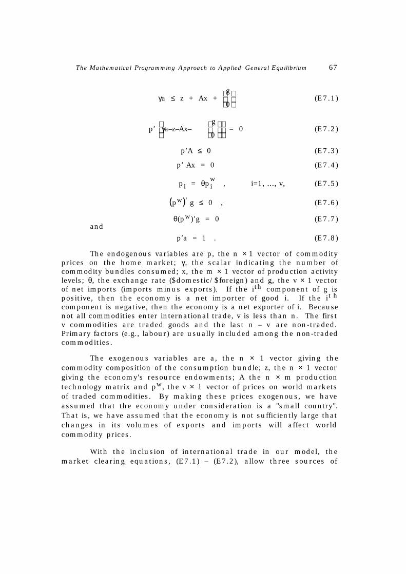
The Mathematical Programming Approach to Applied General Equilibrium 67
γa ≤ z + Ax +
g
0 (E7.1)
p′
γa–z–Ax–
g
0 = 0 (E7.2)
p′A ≤ 0 (E7.3)
p′ Ax = 0 (E7.4)
pi = θpwi , i=1, ..., v, (E7.5)
(pw)′ g ≤ 0 , (E7.6)
θ(pw) ′g = 0 (E7.7)and
p′a = 1 . (E7.8)
The endogenous variables are p, the n × 1 vector of commodityprices on the home market; γ, the scalar indicating the number ofcommodity bundles consumed; x, the m × 1 vector of production activitylevels; θ, the exchange rate ($domestic/$foreign) and g, the v × 1 vectorof net imports (imports minus exports). If the ith component of g ispositive, then the economy is a net importer of good i. If the it h
component is negative, then the economy is a net exporter of i. Becausenot all commodities enter international trade, v is less than n. The firstv commodities are traded goods and the last n – v are non-traded.Primary factors (e.g., labour) are usually included among the non-tradedcommodities.
The exogenous variables are a, the n × 1 vector giving thecommodity composition of the consumption bundle; z, the n × 1 vectorgiving the economy's resource endowments; A the n × m productiontechnology matrix and pw, the v × 1 vector of prices on world marketsof traded commodities. By making these prices exogenous, we haveassumed that the economy under consideration is a "small country".That is, we have assumed that the economy is not sufficiently large thatchanges in its volumes of exports and imports will affect worldcommodity prices.
With the inclusion of international trade in our model, themarket clearing equations, (E7.1) – (E7.2), allow three sources of

68 Peter B. Dixon
supply: the resource endowment, production and net imports.20 Thezero-pure-profits conditions, (E7.3) – (E7.4), are as in earlier exercises.Condition (E7.5) says that domestic prices for traded commodities aredetermined by translating world prices into domestic currency via theexchange rate. If the exchange rate is $0.9 domestic per $1 foreign andp
wi = $10 foreign, then the local price, pi, for commodity i will be $9
domestic. No one in the local economy would be willing to pay morethan $9 domestic for a unit of good i since it can be obtained for thatprice through importing. On the other hand, no one in the localeconomy would be willing to sell a unit of good i for less than $9domestic since this much could be obtained through exporting. Ofcourse, (E7.5) assumes that there are no transport costs, import dutiesor other impediments to trade. Conditions (E7.6) and (E7.7) are themarket clearing equations for foreign currency. Net demand for foreigncurrency (the balance of trade deficit) must be less than or equal tozero. If net demand is negative, then the price of foreign currency (θ)will be zero. Condition (E7.8) sets the absolute price level.
(a) For (p_, γ_, x
_, θ_, g
_) satisfying (E7.1) – (E7.8) show that
p_
′ γ_a = p
_′ z .
That is, show that final expenditure equals income.
(b) Assume that
a =
3
2
0
, z =
0
0
200
, A =
1.0 –0.2
–0.4 1.0
–1.0 –2.0
and pw =
2
1 .
Find the equilibrium values for p, γ, x, θ and g.
(c ) Write a linear programming problem which would be a suitablevehicle for solving (E7.1) – (E7.8).
20 The "0" appearing in the net-import terms of (E7.1) and (E7.2) is a vector of n– v zeros.

The Mathematical Programming Approach to Applied General Equilibrium 69
(d) Show that if the model (E7.1) – (E7.8) has a solution, then it hasa solution in which no more than n – v components of x are non-zero. In an empirical application of the model, would you expectto find solutions in which more than n – v of the productionactivities were operated at positive levels?
(e ) Models similar to (E7.1) – (E7.8) often imply unrealistic levels ofindustrial specialization. Discuss this in the light of your findingin part (d). What real world factors explaining industrialdiversification are left out of the model (E7.1) – (E7.8)? Noanswer is provided for this question. In checking your answer,you might find it useful to read Dixon and Butlin (1977, sectionIII, pp. 342-344).
Answer to Exercise 7
(a) From (E7.2) and (E7.5) we have
p_
′ γ_a – p
_′ z – p
_′ Ax
_ – θ
_(pw) ′ g
_ = 0 .
On using (E7.4) and (E7.7), we obtain the required result.
(b) Equilibrium prices must satisfy
(p1, p2, p3)
1.0 –0.2
–0.4 1.0
–1.0 –2.0
≤ (0, 0) . (E7.9)
This can be reduced to21
(2, 1, p3/θ)
1.0 –0.2
–0.4 1.0
–1.0 –2.0
≤ (0, 0) . (E7.10)
We assume that at least one of the two production activities is operatedat a non-zero level. Thus we look for a value for p3/θ such that
21 We may assume that θ ≠ 0. If θ were zero, then p1 and p2 would be zero.Given that a′ = (3, 2, 0), we would have p′a = 0, violating (E7.8).
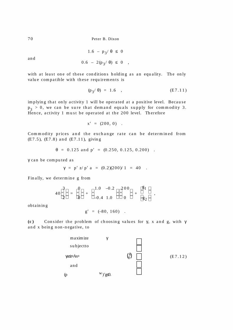
70 Peter B. Dixon
1.6 – p3/θ ≤ 0
and0.6 – 2(p3/θ) ≤ 0 ,
with at least one of these conditions holding as an equality. The onlyvalue compatible with these requirements is
(p3/θ) = 1.6 , (E7.11)
implying that only activity 1 will be operated at a positive level. Becausep3 > 0, we can be sure that demand equals supply for commodity 3.Hence, activity 1 must be operated at the 200 level. Therefore
x′ = (200, 0) .
Commodity prices and the exchange rate can be determined from(E7.5), (E7.8) and (E7.11), giving
θ = 0.125 and p′ = (0.250, 0.125, 0.200) .
γ can be computed as
γ = p′ z/p′ a = (0.2)(200)/1 = 40 .
Finally, we determine g from
40
3
2 =
0
0 +
1.0 –0.2
–0.4 1.0
200
0 +
g1
g2
,
obtainingg′ = (–80, 160) .
(c) Consider the problem of choosing values for γ, x and g, with γand x being non-negative, to
maximize γ
subjectto
γa≤z+Ax+ (g0)
and
(p w) ′g≤0.
(E7.12)

The Mathematical Programming Approach to Applied General Equilibrium 71
If (γ_, x
_, g
_ ) is a solution to this problem, then there exists p
_ ≥ 0 and θ
_ ≥ 0
such that
1 – p_
′ a = 0 , (E7.13)22
p_
′ A ≤ 0 , (E7.14)
p_
′ Ax_ = 0 , (E7.15)
p_
i = θ_p
wi , i=1, ..., v, (E7.16)23
γ_a ≤ z + Ax
_ +
g
_
0 , (E7.17)
p_
′
γ
_a–z–Ax
_–
g
_
0 = 0 , (E7.18)
(pw) ′ g_ ≤ 0 (E7.19)
and
θ_(pw) ′ g
_ = 0 . (E7.20)
Thus {p_, γ_, x
_, θ
_, g
_} satisfies the conditions (E7.1) – (E7.8). This means
that solutions for the model (E7.1) – (E7.8) can be computed by solvingthe linear programming problem (E7.12), together with the associateddual problem.
Alternatively, we could solve a smaller linear programmingproblem:
choose non-negative values for γ and x
to maximize γ
22 We assume that γ_ > 0.
23 Remember that g is not restricted with respect to sign. Consequently (E7.16)is an equality.
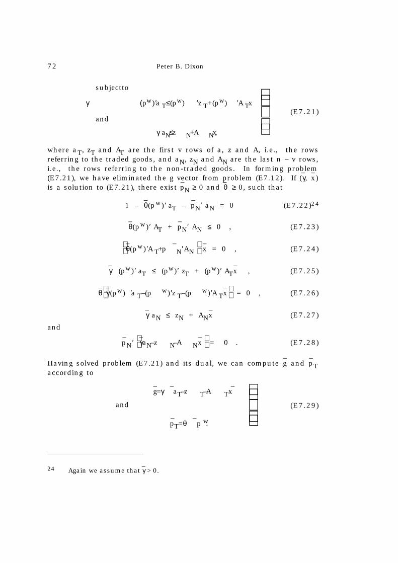
72 Peter B. Dixon
subjectto
γ (pw) ′a T≤(pw) ′z T+(pw) ′A Tx
and
γ aN≤z N+A Nx,
(E7.21)
where aT, zT and AT are the first v rows of a, z and A, i.e., the rowsreferring to the traded goods, and aN, zN and AN are the last n – v rows,i.e., the rows referring to the non-traded goods. In forming problem(E7.21), we have eliminated the g vector from problem (E7.12). If (γ
_, x
_)
is a solution to (E7.21), there exist p_
N ≥ 0 and θ_ ≥ 0, such that
1 – θ_(pw) ′ aT – p
_
N′ aN = 0 (E7.22)24
θ_(pw) ′ AT + p
_
N′ AN ≤ 0 , (E7.23)
θ
_(pw) ′A T+p
_
N′AN x_ = 0 , (E7.24)
γ_ (pw) ′ aT ≤ (pw) ′ zT + (pw) ′ ATx
_ , (E7.25)
θ_
γ
_(pw) ′a T–(p w) ′z T–(p w) ′A Tx
_ = 0 , (E7.26)
γ_ aN ≤ zN + ANx
_ (E7.27)
and
p_
N ′
γ
_aN–z N–A Nx
_ = 0 . (E7.28)
Having solved problem (E7.21) and its dual, we can compute g_ and p
_
Taccording to
g
_=γ
_aT–z T–A Tx
_
and
p_
T=θ_p w.
(E7.29)
24 Again we assume that γ_ > 0.

The Mathematical Programming Approach to Applied General Equilibrium 73
We see that { (p_ ′
T, p_ ′
N) ′, γ_, x
_, θ
_, g
_} is a solution to the model (E7.1) –
(E7.8). Hence the model can be solved by using the linear programmingproblem (E7.21) and the post-solution computations, (E7.29).
(d) Let {p_, γ
_, x
_, θ
_, g
_} be a solution to the model (E7.1) – (E7.8).
Then the linear programming problem (E7.21) has a solution. In fact( γ_, x
_) is a solution.25 Since (E7.21) has a solution, it must have a basic
solution.26 The number of non-zero variables in a basic solution is nomore than the number of constraints. Thus, problem (E7.21) has asolution with no more than 1 + n – v variables at non-zero levels. We canassume that solutions to (E7.21) have a positive value for γ. We concludethat (E7.21) has a solution in which no more than n – v of thecomponents of x are non-zero. Because any solution to (E7.21),together with the associated dual solution and the post-solutioncomputations (E7.29), provides a solution to the model (E7.1) – (E7.8),we have shown that if the model has a solution then it has a solution inwhich no more than n - v of the production activities are operated.
In an empirical application of the model (E7.1) – (E7.8) it wouldbe considered an unlikely accident if there were any solutions withmore than n– v production activities at non-zero levels. To see why,consider the problem of finding values for θ
_ and p
_
N to satisfy
( θ_, p
_
N ′)
(pw) ′A*
T (p_w) ′aT
A*N aN
= (0 ′, 1) (E7.30)
where A* is formed by selecting columns of A and A*T consists of the
first v rows of A* and A*N consist of the remaining (n – v) rows. If A*
contains more than n – v columns, then the system (E7.30) has moreequations than variables. In this circumstance, it would be surprising ifit had a solution. It is reasonable to assume that (E7.30) has no solutionfor any choice of A* having more than n – v columns. Under thisassumption, the model (E7.1) – (E7.8) could not have a solution with
25 Conditions (E7.22) – (E7.28) are both necessary and sufficient for a solutionof (E7.21). See parts 1 and 2 of the Appendix.
26 See parts 3 – 5 of the Appendix .
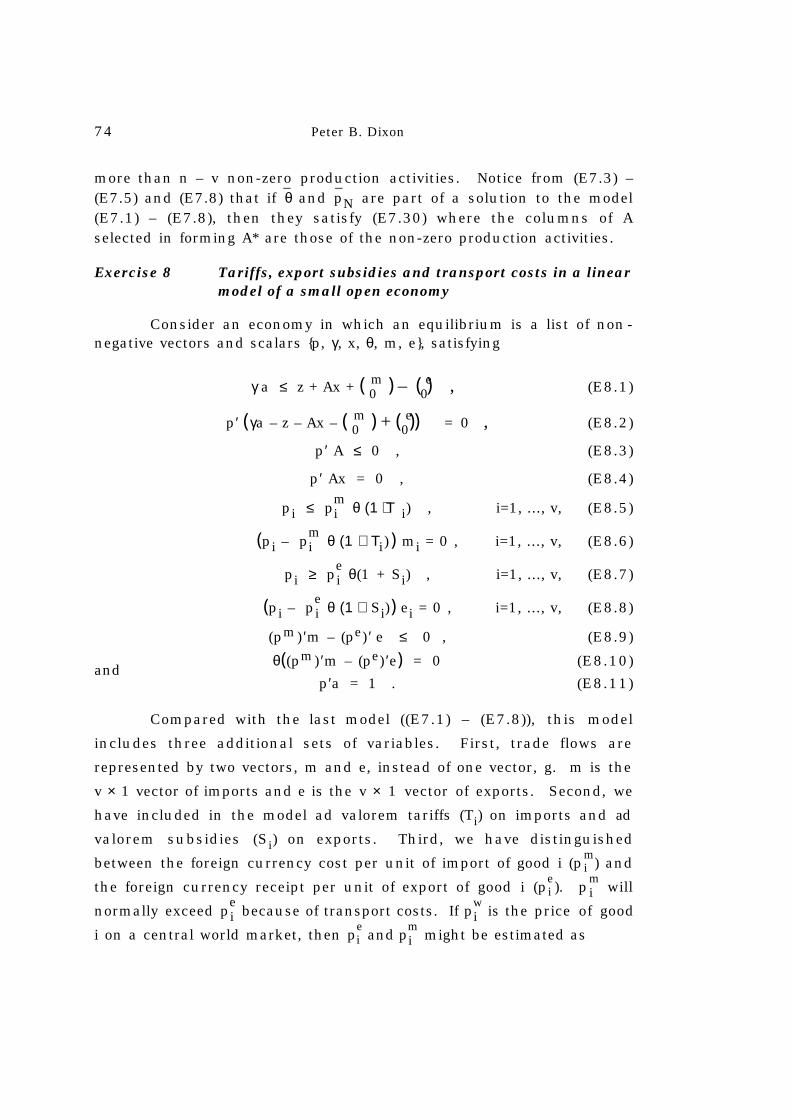
74 Peter B. Dixon
more than n – v non-zero production activities. Notice from (E7.3) –(E7.5) and (E7.8) that if θ
_ and p
_
N are part of a solution to the model(E7.1) – (E7.8), then they satisfy (E7.30) where the columns of Aselected in forming A* are those of the non-zero production activities.
Exercise 8 Tariffs, export subsidies and transport costs in a linearmodel of a small open economy
Consider an economy in which an equilibrium is a list of non -negative vectors and scalars {p, γ, x, θ, m, e}, satisfying
γ a ≤ z + Ax + ( m0 ) – ( e
0) , (E8.1)
p′ (γa – z – Ax – ( m0 ) + ( e
0)) = 0 , (E8.2)
p′ A ≤ 0 , (E8.3)
p′ Ax = 0 , (E8.4)
pi ≤ pmi θ (1 + Τi) , i=1, ..., v, (E8.5)
(pi – pmi θ (1 + Τi) ) mi = 0 , i=1, ..., v, (E8.6)
pi ≥ pei θ(1 + Si) , i=1, ..., v, (E8.7)
(pi – pei θ (1 + Si) ) ei = 0 , i=1, ..., v, (E8.8)
(pm) ′m – (pe) ′ e ≤ 0 , (E8.9)
θ((pm) ′m – (pe) ′e) = 0 (E8.10)and
p′a = 1 . (E8.11)
Compared with the last model ((E7.1) – (E7.8)), this model
includes three additional sets of variables. First, trade flows are
represented by two vectors, m and e, instead of one vector, g. m is the
v × 1 vector of imports and e is the v × 1 vector of exports. Second, we
have included in the model ad valorem tariffs (Ti) on imports and ad
valorem subsidies (Si) on exports. Third, we have distinguished
between the foreign currency cost per unit of import of good i (pmi ) and
the foreign currency receipt per unit of export of good i (pei ). p
mi will
normally exceed pei because of transport costs. If p
wi is the price of good
i on a central world market, then pei and p
mi might be estimated as
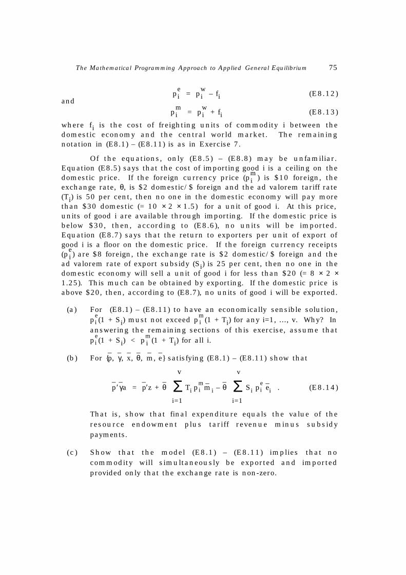
The Mathematical Programming Approach to Applied General Equilibrium 75
pei = p
wi – fi (E8.12)
and
pmi = p
wi + fi (E8.13)
where fi is the cost of freighting units of commodity i between thedomestic economy and the central world market. The remainingnotation in (E8.1) – (E8.11) is as in Exercise 7.
Of the equations, only (E8.5) – (E8.8) may be unfamiliar.Equation (E8.5) says that the cost of importing good i is a ceiling on thedomestic price. If the foreign currency price (p
mi ) is $10 foreign, the
exchange rate, θ, is $2 domestic/$ foreign and the ad valorem tariff rate(Ti) is 50 per cent, then no one in the domestic economy will pay morethan $30 domestic (= 10 × 2 × 1.5) for a unit of good i. At this price,units of good i are available through importing. If the domestic price isbelow $30, then, according to (E8.6), no units will be imported.Equation (E8.7) says that the return to exporters per unit of export ofgood i is a floor on the domestic price. If the foreign currency receipts(p
ei ) are $8 foreign, the exchange rate is $2 domestic/$ foreign and the
ad valorem rate of export subsidy (Si) is 25 per cent, then no one in thedomestic economy will sell a unit of good i for less than $20 (= 8 × 2 ×1.25). This much can be obtained by exporting. If the domestic price isabove $20, then, according to (E8.7), no units of good i will be exported.
(a) For (E8.1) – (E8.11) to have an economically sensible solution,p
ei (1 + Si) must not exceed p
mi (1 + Ti) for any i=1, ..., v. Why? In
answering the remaining sections of this exercise, assume thatp
ei (1 + Si) < p
mi (1 + Ti) for all i.
(b) For {p_, γ
_, x
_, θ
_, m
_, e_} satisfying (E8.1) – (E8.11) show that
p_
′ γ_a = p
_′z + θ
_ Σi=1
v
Ti pmi m
_i – θ
_ Σi=1
v
Si pei e
_i . (E8.14)
That is, show that final expenditure equals the value of theresource endowment plus tariff revenue minus subsidypayments.
(c ) Show that the model (E8.1) – (E8.11) implies that nocommodity will simultaneously be exported and importedprovided only that the exchange rate is non-zero.
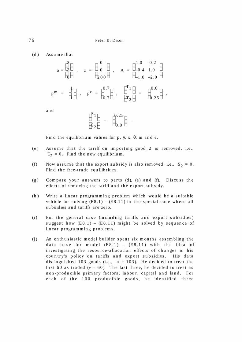
76 Peter B. Dixon
(d) Assume that
a =
3
2
0
, z =
0
0
200
, A =
1.0 –0.2
–0.4 1.0
–1.0 –2.0
pm =
1
1 , pe =
0.7
0.7 ,
T1
T2
=
0.0
0.25 ,
and
S1
S2
=
0.25
0.0 .
Find the equilibrium values for p, γ, x, θ, m and e.
(e ) Assume that the tariff on importing good 2 is removed, i.e., T2 = 0. Find the new equilibrium.
(f) Now assume that the export subsidy is also removed, i.e., S2 = 0.Find the free-trade equilibrium.
(g) Compare your answers to parts (d), (e) and (f). Discuss theeffects of removing the tariff and the export subsidy.
(h) Write a linear programming problem which would be a suitablevehicle for solving (E8.1) – (E8.11) in the special case where allsubsidies and tariffs are zero.
(i ) For the general case (including tariffs and export subsidies)suggest how (E8.1) – (E8.11) might be solved by sequence oflinear programming problems.
(j) An enthusiastic model builder spent six months assembling thedata base for model (E8.1) – (E8.11) with the idea ofinvestigating the resource-allocation effects of changes in hiscountry's policy on tariffs and export subsidies. His datadistinguished 103 goods (i.e., n = 103). He decided to treat thefirst 60 as traded (v = 60). The last three, he decided to treat asnon-producible primary factors, labour, capital and land. Foreach of the 100 producible goods, he identified three

The Mathematical Programming Approach to Applied General Equilibrium 77
techniques of production. Thus, the dimensions of his A matrixwere an impressive 103 × 300.
To solve the model he applied the algorithm described in ouranswer to part (i) using an efficient linear programming package.The computations went without a hitch. By spending only a fewdollars of his research grant at the computer centre, hegenerated model solutions for an enormous variety of tariff andsubsidy policies.
Unfortunately his results seemed very unrealistic. He noted thathis model never showed more than three commodities withpositive export levels. In those solutions where there werethree exports, there were no commodities which were bothimported and domestically produced and none which wereobtained by more than one production technique. In manysolutions there were less than three exported commodities. Insome of these, one or two commodities were both imported anddomestically produced and occasionally there were one or twocommodities produced by more than one technique. In anumber of the solutions where there were less than threeexports, one or two of the primary factors were left in excesssupply implying that their wage rates (prices) were zero. Canyou explain these results?
Answer to Exercise 8
(a) If pei (1 + Si) were greater than p
mi (1 + Ti), then in any solution
to the model θ would have to be zero. Otherwise (E8.5) and (E8.7)could not be satisfied. Thus, if our model had any solution at all, itwould be a solution in which the domestic prices of all traded goods(goods 1, ..., v) were zero. Intuitively, the problem is that if p
ei (1 + Si)
exceeds pmi (1 + Ti) and θ is greater than zero, then profits are available
simply by importing units of good i and re-exporting them.
(b) From (E8.2), we have
p_
′ γ_a = p
_′z + p
_′Ax
_ + Σ
i=1
v
p_
i m_
i – Σi=1
v
p_
i e_
i .
On using (E8.4), (E8.6), (E8.8) and (E8.10), we obtain (E8.14).
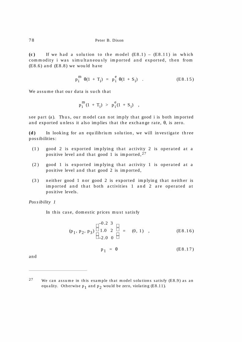
78 Peter B. Dixon
(c) If we had a solution to the model (E8.1) – (E8.11) in whichcommodity i was simultaneously imported and exported, then from(E8.6) and (E8.8) we would have
pmi θ(1 + Ti) = p
ei θ(1 + Si) . (E8.15)
We assume that our data is such that
pmi (1 + Ti) > p
ei (1 + Si) ,
see part (a). Thus, our model can not imply that good i is both importedand exported unless it also implies that the exchange rate, θ, is zero.
(d) In looking for an equilibrium solution, we will investigate threepossibilities:
(1 ) good 2 is exported implying that activity 2 is operated at apositive level and that good 1 is imported,27
(2) good 1 is exported implying that activity 1 is operated at apositive level and that good 2 is imported,
(3) neither good 1 nor good 2 is exported implying that neither isimported and that both activities 1 and 2 are operated atpositive levels.
Possibility 1
In this case, domestic prices must satisfy
(p1, p2, p3)
–0.2 3
1.0 2
–2.0 0
= (0, 1) , (E8.16)
p1 = θ (E8.17)
and
27 We can assume in this example that model solutions satisfy (E8.9) as anequality. Otherwise p1 and p2 would be zero, violating (E8.11).
The Mathematical Programming Approach to Applied General Equilibrium 79
p2 = 0.7θ . (E8.18)
Condition (E8.16) imposes zero profits in activity 2 and sets theabsolute price level according to (E8.11). Conditions (E8.17) and(E8.18) recognize that commodity 1 is imported and commodity 2 isexported.
From (E8.16) – (E8.18) we find that
θ = 0.227 , p1 = 0.227 , p2 = 0.159 and p3 = 0.057 .
On these prices, however, activity 1 could be operated at positive profit:
Profit per unit of activity 1 = 0.227 – (0.159) (0.4) – 0.057
= 0.106 .
We may conclude that there is no equilibrium solution with commodity2 being exported.
Possibility 2
In this case, domestic prices must satisfy
(p1, p2, p3)
1.0 3
–0.4 2
–1.0 0
= (0, 1) , (E8.19)
p1 = 0.7θ(1.25)
andp2 = θ(1.25) .
This gives
θ = 0.195, p1 = 0.171, p2 = 0.244 and p3 = 0.073 .
These prices are inconsistent with the condition that profits are non -positive per unit of activity 2:
profit per unit of activity 2 = – (0.171) (0.2) + 0.244 – (0.073)(2)
= 0.064 .
We may conclude that there is no equilibrium solution with commodity1 being exported.
Possibility 3

80 Peter B. Dixon
Because both activities are operated, prices must satisfy
(p1, p2, p3)
1.0 –0.2 3
–0.4 1.0 2
–1.0 –2.0 0
= (0, 0, 1) ,
i.e.,(p1, p2, p3) = (0.183, 0.225, 0.094) . (E8.20)
With neither good being exported (and therefore neither beingimported) and with non-zero prices, (E8.1) and (E8.2) imply that
3
2
0
γ =
0
0
200
+
1.0 –0.2
–0.4 1.0
–1.0 –2.0
x1
x2
,
i.e., x1 = 69.4, x2 = 65.3 and γ = 18.8 . (E8.21)
Finally, if domestic prices are to be given by (E8.20), then theexchange rate θ must be consistent with
0.7 θ(1.25)≤0.183≤ θand
0.7 θ≤0.225≤θ(1.25) ,(E8.22)
where the conditions (E8.22) specify the ceilings and floors ondomestic prices of traded commodities provided by the availability ofimport supplies and export markets. θ will satisfy (E8.22) if and only if
θ >_ max
0.183,0.2251.25 = 0.183
and
θ ≤ min
0.183
(0.7)(1.25),0.2250.7 = 0.209 .
In summary, the conditions for an equilibrium are satisfied if
0.183 ≤ θ ≤ 0.209 , (E8.23)
m = e = 0 ,and
p, γ and x are given by (E8.20) and (E8.21).

The Mathematical Programming Approach to Applied General Equilibrium 81
Equilibrium values for p, γ, x, m and e are uniquely determined in thisexample. On the other hand, equilibrium values for the exchange rateoccur throughout the range specified by (E8.23).
(e) We investigate the three possibilities set out in our answer to (d).
82 Peter B. Dixon
Possibility 1
Possibility 1 produces no equilibrium solutions. The arithmetichere is exactly the same as that under possibility 1 of part (d).
Possibility 2
In this case, domestic prices must satisfy (E8.19) and
p1 = 0.7θ(1.25)
and
p2 = θ .
This gives
θ = 0.216, p1 = 0.189, p2 = 0.216 and p3 = 0.102. (E8.24)
We note that these prices are consistent with profits per unit ofoperation of activity 2 being non-positive:
profit per unit of activity 2 = – (0.189) (0.2) + 0.216 – (0.102) (2.0)
= – 0.026 .
With prices and the exchange rate being non-zero and theoperation of activity 2 and the level of exports of good 2 being zero,(E8.1), (E8.2) and (E8.10) imply that
3
2
0
γ =
0
0
200
+
1.0
–0.4
–1.0 x1 +
–e1
m2
0and that
m2 – 0.7e1 = 0 .
This gives
x1 = 200, γ = 14.6, e1 = 156.1, m2 = 109.3 . (E8.25)
(E8.24) and (E8.25) together with the conditions e2 = m1 = x2 = 0, arean equilibrium solution.
Possibility 3
The Mathematical Programming Approach to Applied General Equilibrium 83
If both activities are operated, then prices must be given by(E8.20) and the exchange rate must satisfy
0.7 θ(1.25)≤0.183≤ θ
0.7 θ≤0.225≤ θ.(E8.26)
θ will satisfy (E8.26) if and only if
θ >_ max{0.183 , 0.225} = 0.225and
θ ≤ min
0.183
(0.7)(1.25),0.225
0.7 = 0.209 .
Since there is no value for θ consistent with these last two conditions,there is no equilibrium solution with both activities operated at positivelevels. Hence, there is no equilibrium solution in which neither good isexported.
We conclude that the only equilibrium solution is that locatedunder possibility 2, i.e.,
p =
0.189
0.216
0.102
, γ = 14.6, x =
200
0 , θ = 0.216,
m =
0
109.3 , e =
156.1
0 .
(f) Again we investigate the three possibilities.
Possibility 1
As in parts (d) and (e), possibility 1 produces no equilibriumsolutions.
Possibility 2
In this case, domestic prices must satisfy (E8.19) and
p1 = 0.7θ
and
p2 = θ .This gives
θ = 0.244, p1 = 0.171, p2 = 0.244 and p3 = 0.073 .
84 Peter B. Dixon
At these prices, activity 2 can be operated at a profit. Thus, possibility 2produces no solutions in this example.
Possibility 3
We follow the answer to part (d) under possibility 3 to establishthat prices must satisfy (E8.20) and quantities must satisfy (E8.21).
The exchange rate, θ, must be consistent with
0.7θ≤0.183≤θ
and
0.7θ≤0.225≤ θ.
(E8.27)
θ will satisfy (E8.27) if and only if
θ >_ max {0.183 , 0.225} = 0.225and
θ ≤ min
0.183
0.7 ,0.2250.7 = 0.261 .
Thus, the conditions for an equilibrium are satisfied if
0.225 ≤ θ ≤ 0.261 ,
m = e = 0and
p, γ and x are given by (E8.20) and (E8.21).
(g) Table E8.1 lists the solutions obtained in parts (d), (e) and (f).These illustrate two general propositions. First, the deterioration inwelfare (measured by γ) as we move from the first solution to the secondillustrates Lipsey and Lancaster's (1957) famous second-best result. Theremoval of one distortion (the tariff) does not necessarily improvewelfare in a situation where other distortions (the subsidy) remain.28
However, the removal of the subsidy in a situation where it is the
28 Hazari (1978) is an authoritative and readable text on the welfare effects ofpolicy changes in an open economy with distortions.
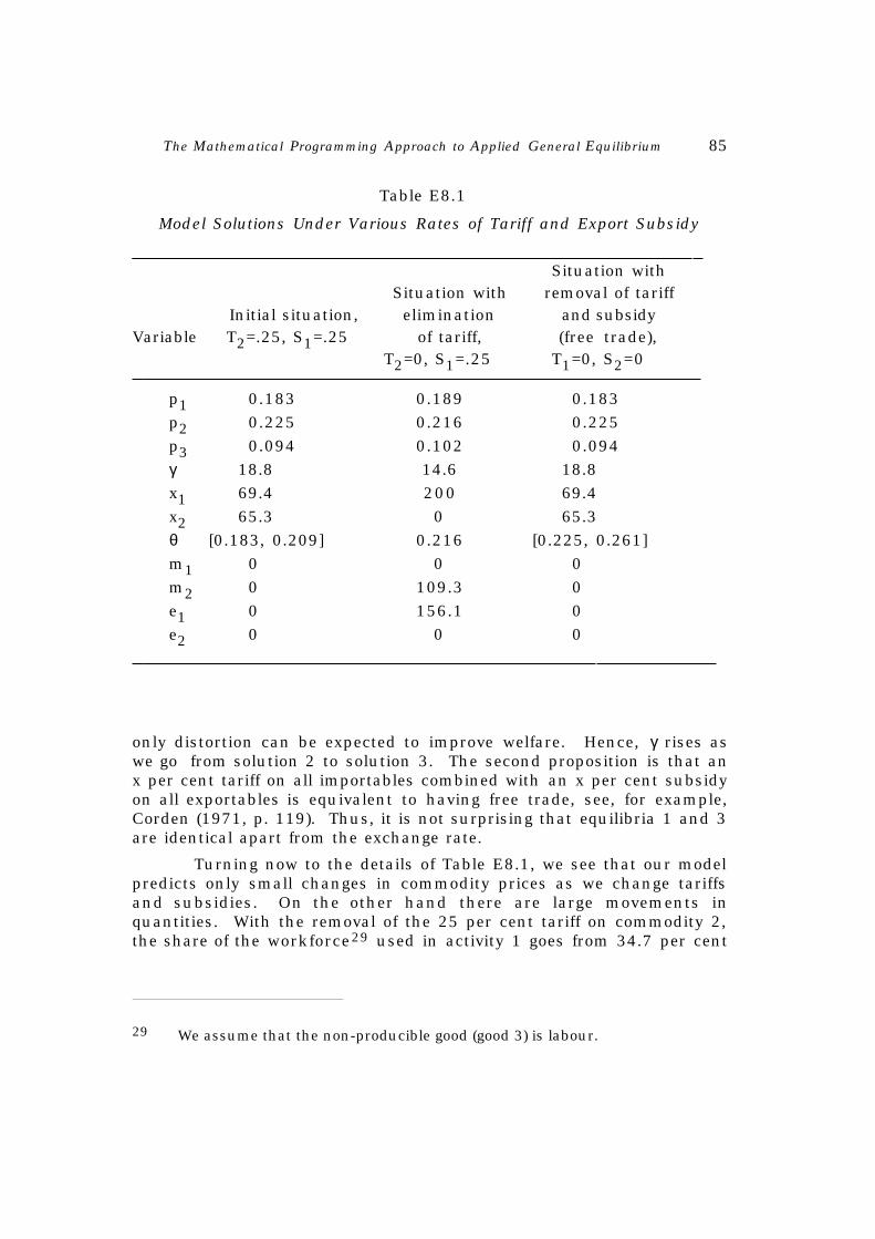
The Mathematical Programming Approach to Applied General Equilibrium 85
Table E8.1
Model Solutions Under Various Rates of Tariff and Export Subsidy
Situation with
Situation with removal of tariffInitial situation, elimination and subsidy
Variable T2=.25, S1=.25 of tariff, (free trade),T2=0, S1=.25 T1=0, S2=0
p1 0.183 0.189 0.183
p2 0.225 0.216 0.225
p3 0.094 0.102 0.094
γ 18.8 14.6 18.8
x1 69.4 200 69.4
x2 65.3 0 65.3
θ [0.183, 0.209] 0.216 [0.225, 0.261]
m1 0 0 0
m2 0 109.3 0
e1 0 156.1 0
e2 0 0 0
only distortion can be expected to improve welfare. Hence, γ rises aswe go from solution 2 to solution 3. The second proposition is that anx per cent tariff on all importables combined with an x per cent subsidyon all exportables is equivalent to having free trade, see, for example,Corden (1971, p. 119). Thus, it is not surprising that equilibria 1 and 3are identical apart from the exchange rate.
Turning now to the details of Table E8.1, we see that our modelpredicts only small changes in commodity prices as we change tariffsand subsidies. On the other hand there are large movements inquantities. With the removal of the 25 per cent tariff on commodity 2,the share of the workforce29 used in activity 1 goes from 34.7 per cent
29 We assume that the non-producible good (good 3) is labour.
86 Peter B. Dixon
to 100 per cent. The ratio of the value of exports to GDP 30 goes from 0to 2.02 (i.e., (156.1)(0.189)/14.6) and consumption falls in real termsby 22.3 per cent (18.8 to 14.6). Consumption has fallen despite thesmall rise in the wage rate (p3 ). This is because disposable factorincome has been reduced by the need to provide for the export subsidy(see equation (E8.14)).
The volatility of the quantity results reflects the lack ofdiversifying phenomena in our model, see Exercise 7(e). The modelomits terms of trade effects and this particular example includes noactivity-specific non-producible factors, e.g. agricultural land, skilledlabour or mines. The example has only one non-producible factor andthis is assumed to be perfectly mobile across activities.
(h) Consider the linear programming problem of choosing non -negative values for γ, x, m and e to
maximize γ
subjectto
γa≤z+Ax+
m
0–
e
0
and
(pm)′m–(p e)′e≤0.
(E8.28)
The list of non-negative vectors and scalars, {γ_, x
_, m
_, e
_}, is a solution to
this problem if and only if there exists p_ ≥ 0, θ
_ ≥ 0 such that
1 – p_ ′a = 0 , (E8.29)31
p_ ′A ≤ 0 , (E8.30)
p_ ′Ax
_ = 0 , (E8.31)
30 With the trade balance assumed to be zero, see (E8.10), and with pricesnormalized accordingly to (E8.11), GDP in this model is the number ofconsumption bundles, i.e. GDP is γ.
31 We assume that γ_ > 0 so that (E8.29) can be written as an equality.

The Mathematical Programming Approach to Applied General Equilibrium 87
p_
i – θ_ p
mi ≤ 0 , i=1, ..., v, (E8.32)
(p_
i – θ_ p
mi )m
_
i = 0 , i=1, ..., v, (E8.33)
–p_ i + θ
_p
ei ≤ 0 , i=1, ..., v, (E8.34)
(–p_
i + θ_p
ei ) e
_ i = 0 , i=1, ..., v, (E8.35)
γ_ a – z – Ax
_ –
m
_
0 +
e
_
0 ≤ 0 , (E8.36)
p_
′
γ_a–z–Ax
_–
m
_
0+
e
_
0 = 0 , (E8.37)
(pm) ′ m_ – (pe) ′ e
_ ≤ 0 (E8.38)
and
θ((pm) ′ m_ – (pe) ′ e
_) = 0 . (E8.39)
Thus, {p_, γ_, x
_, θ
_, m
_, e
_} is a solution to the linear programming problem
(E8.28) and its dual if and only if it satisfies the conditions (E8.1) –(E8.11) for the special case where the Si and Ti are all zeros. Thismeans that all solutions for the free-trade version of the model (E8.1) –(E8.11) can be computed by solving the linear programming problem(E8.28) together with the associated dual problem.
(i) Consider the linear programming problem of choosing non -negative values for γ, x, m and e to maximize
γ – Σi=1
v
pmi ψ Ti mi + Σ
i=1
v
pei ψ Si ei (E8.40)
subject to
γa ≤ z + Ax +
m
0 –
e
0 (E8.41)
and
(pm) ′m – (pe) ′e ≤ 0 . (E8.42)
ψ is an iterative variable. It is varied as we move from one linearprogramming problem to the next, but is held constant as we solve each

88 Peter B. Dixon
problem. As will become apparent, ψ is our guess of an equilibriumvalue for the exchange rate.
The list of non-negative vectors and scalars, {γ_, x
_, m
_, e
_}, is a
solution to the problem (E8.40) – (E8.42) if and only if there exist p_ ≥ 0
and θ_ ≥ 0 such that
1 – p_ ′a = 0 , (E8.43)32
p_ ′A ≤ 0 , (E8.44)
p_ ′Ax
_ = 0 , (E8.45)
–pmi ψ Ti + p
_
i – θ_p
mi ≤ 0, i=1, ..., v, (E8.46)
–p
mi ψTi+p
_
i– θ_p
mi m
_
i = 0, i=1, ..., v, (E8.47)
pei ψ Si – p
_
i + θ_p
ei ≤ 0 , i=1, ..., v, (E8.48)
p
ei ψSi–p
_
i+ θ_p
ei e
_
i = 0, i=1, ..., v, (E8.49)
γ_a – z – Ax
_ –
m
_
0 +
e
_
0 ≤ 0 , (E8.50)
p_
′
γ_a–z–Ax
_–
m
_
0+
e
_
0 = 0 , (E8.51)
(pm) ′ m_ – (pe) ′ e
_ ≤ 0 (E8.52)
and
θ_ ( )(pm) ′m
_–(p e) ′e
_ = 0 . (E8.53)
By comparing (E8.43) – (E8.53) with (E8.1) – (E8.11) we see that{p_, γ_ x_, θ
_, m
_, e
_} is a solution to the model (E8.1) – (E8.11) if
32 Again for convenience, we assume that γ_ > 0. However, we should note that
if ψ were large, it would be possible that the optimal solution to (E8.40) –(E8.42) would imply zero consumption and large volumes of exports to takeadvantage of the subsidy term in the objective function (E8.40).
The Mathematical Programming Approach to Applied General Equilibrium 89
ψ = θ_ . (E8.54)
This suggests that we can solve the model (E8.1) – (E8.11) as follows:first we guess an equilibrium value, ψ(1), for the exchange rate. Then wesolve the linear programming problem (E8.40) – (E8.42) and its dual. Ifthe value, θ
_(1), for the exchange rate emerging from this computation is
equal (or sufficiently close) to ψ(1) then we have found a solution to ourmodel (E8.1) – (E8.11). If ψ (1) ≠ θ
_(1), then we reset the iterative
variable. A rule that is often effective in practice is
ψ(s) = θ_(s–1) , (E8.55)
i.e., we reset the iterative variable for the sth linear programmingproblem according to the value for the exchange rate emerging from the(s–1)th linear program. Of course other adjustment rules could be used,e.g.,
ψ(s) = ψ(s–1) + k( )θ_(s–1)– ψ(s–1) , (E8.56)
where k is greater than zero but less than one. Under (E8.56) we movethe iterative variable only part of the way towards the value for theexchange rate emerging from our latest linear programming solution. Apartial adjustment strategy would be appropriate if cycling became aproblem. Cycling would occur under (E8.55) if, for example, we set ψ(1)
= 1 and obtained θ_(1) = 4, say. Then when we set ψ(2) = 4, we obtain θ
_(2)
= 1. This situation is illustrated in Figure E8.1.
While the possibility of cycling cannot be dismissed, we have notfound it to be a problem in applied work with models similar to (E8.1) –(E8.11). The reason is that the dual variable (θ
_) associated with
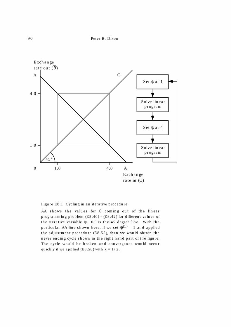
90 Peter B. Dixon
A
4.0
1.0
1.0 4.0 A
45°
C
Exchangerate in (ψ)
Exchangerate out ( θ )
Set ψ at 1
Solve linearprogram
Set ψ at 4
Solve linearprogram
0
Figure E8.1 Cycling in an iterative procedure
AA shows the values for θ coming out of the linearprogramming problem (E8.40) - (E8.42) for different values ofthe iterative variable ψ. 0C is the 45 degree line. With theparticular AA line shown here, if we set ψ(1) = 1 and appliedthe adjustment procedure (E8.55), then we would obtain thenever ending cycle shown in the right hand part of the figure.The cycle would be broken and convergence would occurquickly if we applied (E8.56) with k = 1/2.
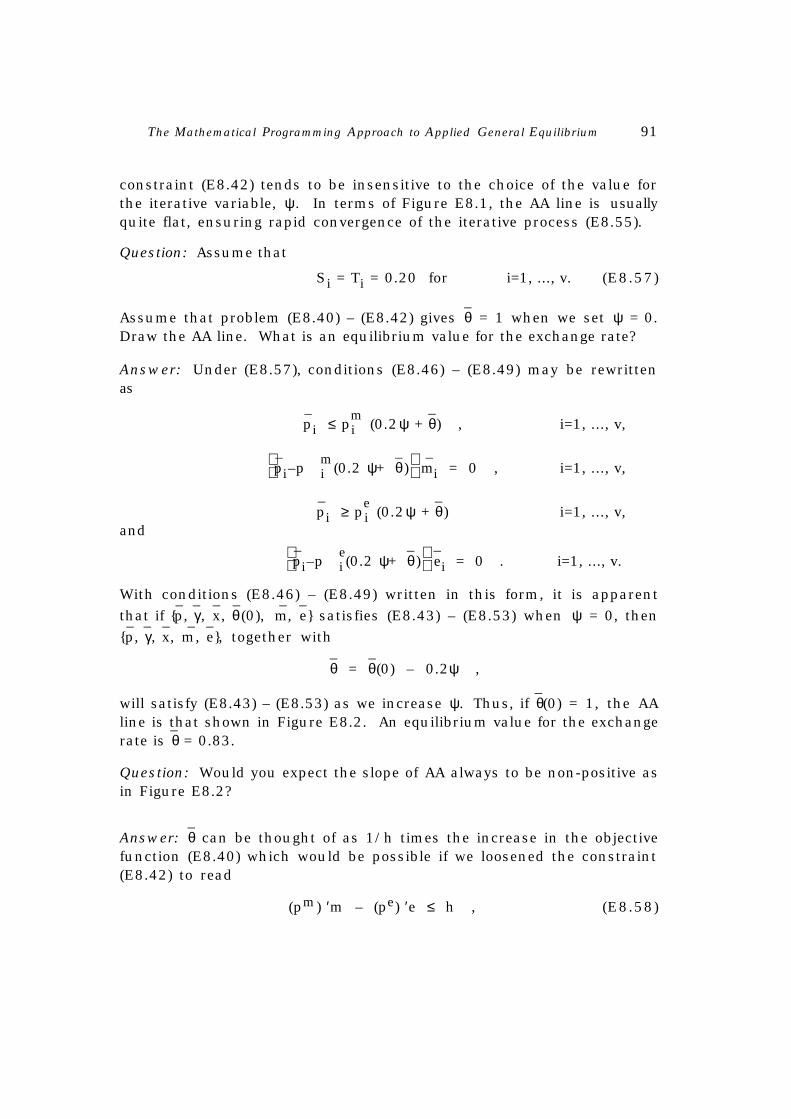
The Mathematical Programming Approach to Applied General Equilibrium 91
constraint (E8.42) tends to be insensitive to the choice of the value forthe iterative variable, ψ. In terms of Figure E8.1, the AA line is usuallyquite flat, ensuring rapid convergence of the iterative process (E8.55).
Question: Assume that
Si = Ti = 0.20 for i=1, ..., v. (E8.57)
Assume that problem (E8.40) – (E8.42) gives θ_ = 1 when we set ψ = 0.
Draw the AA line. What is an equilibrium value for the exchange rate?
Answer: Under (E8.57), conditions (E8.46) – (E8.49) may be rewrittenas
p_
i ≤ pmi (0.2ψ + θ
_) , i=1, ..., v,
p
_
i–pmi (0.2 ψ+ θ
_) m
_
i = 0 , i=1, ..., v,
p_
i ≥ pei (0.2ψ + θ
_) i=1, ..., v,
and
p
_
i–pei (0.2 ψ+ θ
_) e
_
i = 0 . i=1, ..., v.
With conditions (E8.46) – (E8.49) written in this form, it is apparent
that if {p_, γ_, x
_, θ
_(0), m
_, e
_} satisfies (E8.43) – (E8.53) when ψ = 0, then
{p_, γ_, x
_, m
_, e
_}, together with
θ_ = θ
_(0) – 0.2ψ ,
will satisfy (E8.43) – (E8.53) as we increase ψ. Thus, if θ_(0) = 1, the AA
line is that shown in Figure E8.2. An equilibrium value for the exchangerate is θ
_ = 0.83.
Question: Would you expect the slope of AA always to be non-positive asin Figure E8.2?
Answer: θ_ can be thought of as 1/h times the increase in the objective
function (E8.40) which would be possible if we loosened the constraint(E8.42) to read
(pm) ′m – (pe) ′e ≤ h , (E8.58)
92 Peter B. Dixon
where h is chosen to be a small positive number.33 The availability of anextra h units of foreign exchange could be expected to allow increasesin γ via reductions in exports or increases in imports. In terms of theobjective function (E8.40), both increases in imports and reductions inexports become less attractive as we increase ψ . Thus, we wouldnormally expect a negative relationship between θ
_ and ψ.
(j) The model builder solved (E8.1) – (E8.11) using the linearprogramming problem (E8.40) – (E8.42) with an appropriate value forψ. We assume that (E8.40) – (E8.42) has no non-basic solutions. (Evenif there were some non-basic solutions, it is unlikely that the modelbuilder would find them as most linear programming packages producebasic solutions only.) Thus, in his computed solutions the modelbuilder will have no more than 104 (the number of constraints in(E8.41) – (E8.42)) of the 421 variables with non-zero values.34
We assume that γ is one of the variables having a non-zero value.We also assume that model solutions involve non-zero supplies fromproduction or importing of each of the 100 producible goods.35 Hence,for each i=1, ..., 60, at least one of the four variables xi1, xi2, xi3, mi mustbe non-zero where the xij are the activity levels for the three i-producing activities and mi is the import level for good i. For i=61, ...,100, at least one of the three variables xi1, xi2, xi3 is non-zero. This
33 See, for example, Dixon, Bowles and Kendrick (1980, pp. 21-23).
34 The 421 variables are: γ, one variable; x, 300 variables; m, 60 variables ande, 60 variables.
35 This will certainly be true if zi = 0, i=1, ..., 100. That is, the endowments ofthe producible goods are zero.
Th
e Ma
them
atica
l Prog
ram
min
g A
pp
roach
to Ap
plied
Gen
eral E
qu
ilibriu
m 93
AA line with Si = T = 0.2 for i = 1, ...,vi0.83
1.0
0.830 5.0
45°
A
A
C
Exchangerate in (ψ)
Exchangerate out ( θ
_)
the
model (E8.1) – (E8.11)
Figure E8.2 Exchange rate solution in a special case of
reaches zero. As ψ increasesθNote that when _
reaches 5, further, stays at zero and the optimal solutions for problemθ
_
(E8.40) – (E8.42) involve no scarcity of foreign exchange.
Exports are increased to take advantage of the export subsidy
term in the objective function (E8.40) and imports are
reduced to avoid the penalty from the tariff term.
ψ

94 Peter B. Dixon
leaves no more than three other production or trade variables with non-zero values. In particular, no more than three of the ei will be non-zero.
It is not necessary that there be three exported commodities.Two commodities might be exported and one commodity supplied fromtwo sources, either two production activities or one production activityand imports. With two exported commodities, another possibility isthat one primary factor could be left unemployed. In effect, the linearprogramming problem (E8.40) – (E8.42) would then have only 103constraints implying that only 103 variables would appear in thesolution with non-zero values. If only one commodity is exported, thentwo commodities could be supplied from two sources or one commoditycould be supplied from three sources. Alternatively, one or two of theprimary factors might be left in excess supply. A final possibility is thatno commodities are exported. In this case, no commodities will beimported. Two primary factors (but not three) might be left in excesssupply and one commodity supplied by two production techniques, etc.
Exercise 9 A long-run planning model with investment:the snapshot approach
In the snapshot approach, we describe the economy at aparticular point of time in the future. We do this without giving adetailed specification of the time paths of relevant variables. The idea isto construct a simple one period model which can be used to analysethe effects of demographic changes, technological progress and otherlong-run phenomena.
This exercise asks you to set up and analyse a typical (althoughsimplified) snapshot model. You might use the exercise either before orafter you do the reading from Manne (1963), Bruno (1967), Evans(1972) and Sandee (1960). If you choose the first route, you probablywill not be able to do much of the exercise, but by studying the answer,you will get an introduction to the reading. The second route willenable you to check your grasp of the reading. Whichever route youtake, you will notice in the reading that long-run planning models areoften presented in the form of programming problems. In this chapterwe have preferred to present models as sets of conditions definingequilibria. With this approach it is sometimes easier to identify theassumptions being made concerning the behaviour of the economicagents: the households, producers and investors.
The Mathematical Programming Approach to Applied General Equilibrium 95
(a) Imagine that as an economic planner you are asked in 1990 toforecast the output, investment, price and consumptionstructure of Linprogria for the year 2000. The economy ofLinprogria is a simple one. There is no international trade andno government spending or taxes.
Using historical trends revealed from various statisticalsources and information supplied by experts in each industry,you obtain a picture of the likely state of technology in 2000.You present this information in the form of an input-coefficientsmatrix, Q, a labour vector, l, and a capital matrix, K. The typicalelement of Q shows the input of good i which will be used up inthe production of a unit of good j in 2000.36 The typical ele-ment of l is the number of units of labour which will be neededper unit of output of good j and the typical element of K showsthe quantity of good i which will be required in the creation of aunit of capital stock for industry j.37 You define your capitalunits so that 1 unit of capital will be necessary to support a unitof production of good j and you assume that capital is notshiftable, i.e., units of capital created for industry j can only beused in industry j. Also, for simplicity you assume that capitallasts forever, i.e., that there is no depreciation.
Next, you consult with demographers and experts on labourparticipation rates to obtain a forecast, L, for the number oflabour units which will be available in 2000. The demographersalso explain to you the likely age and family structure of the2000 population. You use this information in forming the vector,a, which describes the likely composition of householdconsumption in 2000. The typical element of a is the quantity ofgood i purchased by households per unit of householdexpenditure.
Finally, you make four assumptions concerning thebehaviour of entrepreneurs: first that they are competitive sothat there are no pure profits; second, that they do sufficientinvestment in each industry over the period 1990 to 2000 sothat rates of return on industrial capital in 2000 are no morethan r (10 percent, say) where r is the observed average rate ofreturn on capital over some historical period, for example 1975
36 In this exercise, producible goods and primary factors are treatedseparately. It is also assumed that there are n producible goods and thatthere is one technique or activity for producing each. Q is a non-negative n× n matrix referring to inputs of producible goods.
37 Industry j is the group of firms producing good j.

96 Peter B. Dixon
to 1990; third, that they do no investment in the year 2000 (orover the period 1990 to 2000) in industries having rates ofreturn in 2000 of less than r; and fourth, that they increase thecapital stock in each industry in 2000 sufficiently to maintainthe average rate of growth of capital achieved in the industryfrom 1990 until 2000. This final assumption is a common trickin planning models. Investment in industry j in the final year,2000, is tied down by relating it to the difference between thecapital stock in industry j at the beginning of 2000 (as impliedby the model) and the known current level of capital stockwhich we will denote by kj(90).
Specify your model of 2000 mathematically. You might setout your answer as follows:
The economy in 2000 is described by a list of non-negativescalars, vectors and matrices {x, p, γ, w, Π, J, k(00); Q, l, K, L, a,r, k(90)} satisfying the following set of equations andinequalities,
. . . . . ( i )
. . . . . (ii)...
where
x is the vector of commodity (or industry) outputs;p is the vector of commodity prices;γ is a scalar showing the level of household consum-
ption; i.e., the number of a-vectors consumed;w is the wage rate;Π is the vector of annual rental values of capital stock
in each industry;J is the vector of increases in capital stocks
(investment in 2000);k(00) is the vector of capital stocks by using industry at
the beginning of 2000;(Q, l , K), L, a and r are data for 2000 describing technology, labour
supply, consumer preferences andthe economy-wide rate of return; and
k(90) is the vector of capital stock by using industry at the beginning of 1990.

The Mathematical Programming Approach to Applied General Equilibrium 97
The equations and inequalities should specify that in 2000,demand will not exceed supply for commodities, labour and thecapital stock of each industry; that the prices of commoditiesand primary factors in excess supply will be zero; that aggregateinvestment plus aggregate consumption expenditure will equalaggregate income; that commodity prices will not exceed costs(the zero pure profits assumption); that commodities whoseprices fall short of costs will not be produced; that rates ofreturn (i.e., annual rentals divided by costs of new capital) willnot exceed the historically determined average rate r; thatinvestment will be zero in industries having rates of return ofless than r; and that investment will be sufficient to maintain thegrowth rates of capital in each industry implied by the model for1990 to 2000.
(b) Check that the number of equation equivalents in your model isthe same as the number of endogenous variables. What is therole of homogeneity and Walras' law?
(c ) Suggest an algorithm for computing x, p, γ, w, Π, J, k(00) for agiven data set Q, l, K, L, a, r, k(90). The algorithm should use alinear programming package at each step.
Answer to Exercise 9
(a) The list of endogenous variables
Ξ = {x, p, γ, w, Π, J, k(00)} (E9.1)
will satisfy the equations and inequalities set out below in (E9.2) – (E9.8).
Qx+ γa+KJ≤x
and
p′(Qx+ γa+KJ–x)=0.
(E9.2)
(E9.2) specifies that commodity demands (intermediate, household andinvestment) will not exceed supplies and can only be less than suppliesfor free goods.
l ′x≤L
and
w( l ′x–L)=0.
(E9.3)
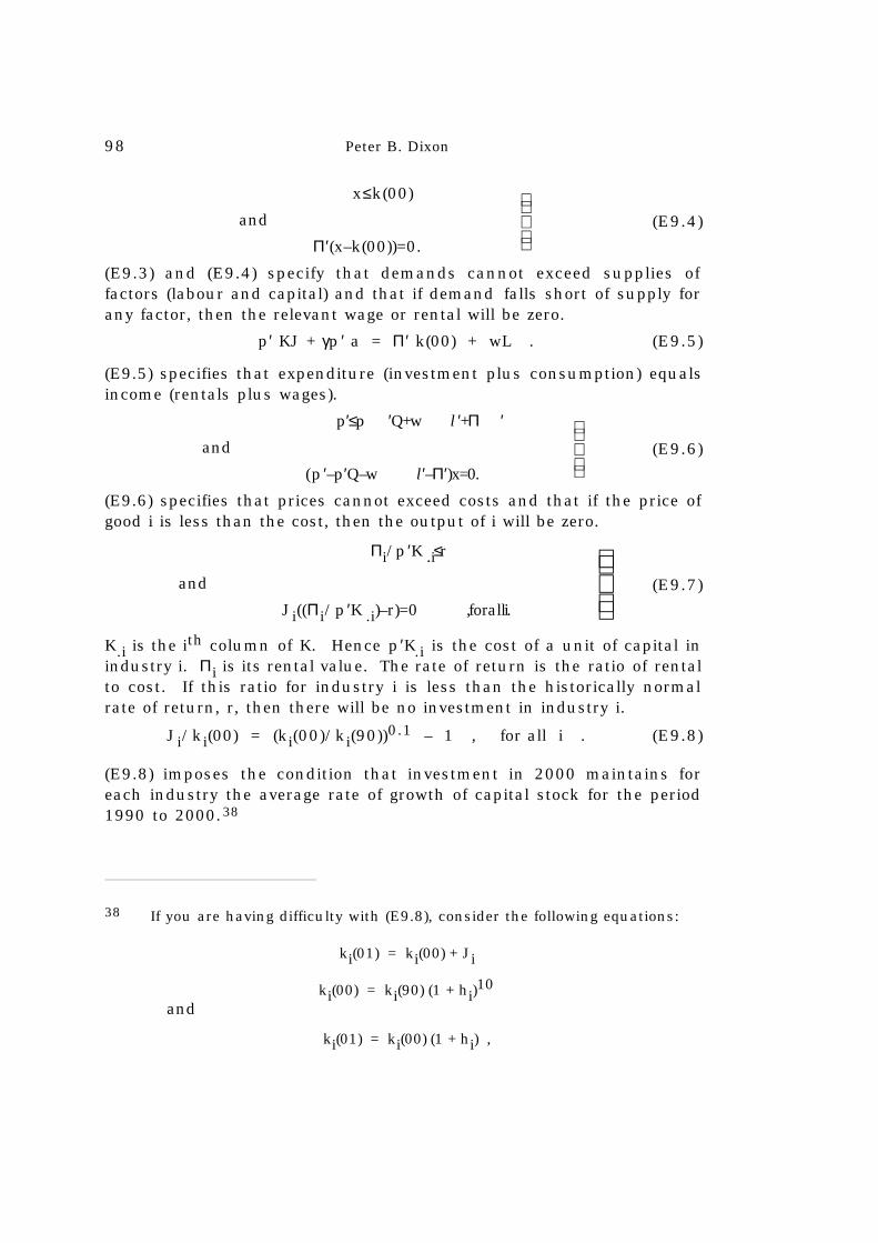
98 Peter B. Dixon
x≤k(00)
and
Π′(x–k(00))=0.
(E9.4)
(E9.3) and (E9.4) specify that demands cannot exceed supplies offactors (labour and capital) and that if demand falls short of supply forany factor, then the relevant wage or rental will be zero.
p′ KJ + γp ′ a = Π′ k(00) + wL . (E9.5)
(E9.5) specifies that expenditure (investment plus consumption) equalsincome (rentals plus wages).
p′≤p ′Q+w l ′+Π ′
and
(p ′–p′Q–w l ′–Π′)x=0.
(E9.6)
(E9.6) specifies that prices cannot exceed costs and that if the price ofgood i is less than the cost, then the output of i will be zero.
Πi/p ′K .i≤r
and
Ji((Πi/p ′K .i)–r)=0 ,foralli.
(E9.7)
K.i is the ith column of K. Hence p ′K.i is the cost of a unit of capital inindustry i. Πi is its rental value. The rate of return is the ratio of rentalto cost. If this ratio for industry i is less than the historically normalrate of return, r, then there will be no investment in industry i.
Ji/ki(00) = (ki(00)/ki(90))0.1 – 1 , for all i . (E9.8)
(E9.8) imposes the condition that investment in 2000 maintains foreach industry the average rate of growth of capital stock for the period1990 to 2000.38
38 If you are having difficulty with (E9.8), consider the following equations:
ki(01) = ki(00) + Ji
ki(00) = ki(90) (1 + hi)10
and
ki(01) = ki(00) (1 + hi) ,

The Mathematical Programming Approach to Applied General Equilibrium 99
(b) Before moving to the question of computations, it is always
reassuring to count equations and variables. Equation counting is not a
complete substitute for a formal discussion of the existence question,
but certainly if we detect a discrepancy between the number of equation
equivalents in (E9.2) – (E9.8) and the number of variables in the list Ξ(see (E9.1)) we will have doubts about either the completeness or
internal consistency of our description of 2000.
Where n is the number of goods, we see that Ξ contains n + n +
1 + 1 + n + n + n = 5n + 2 variables. Conditions (E9.2) – (E9.8) are
equivalent to n + 1 + n + 1 + n + n + n = 5n + 2 equations. 39 But what
about homogeneity and Walras’ law? We consider homogeneity. It is
clear that our description of 2000 says nothing about the absolute price
level. If we have found a list Ξ1 = {x_, p
_, γ
_, w
_, Π
_, J
_, k
_(00)} which
satisfies (E9.2) – (E9.8), then Ξ2 = {x_, λp
_, γ
_, λw
_, λ Π
_, J
_, k
_(00)} also
satisfies (E9.2) – (E9.8) where λ is any positive scalar. To remove the
indeterminacy, we can fix the absolute price level by adding an equation
such as
p′a = 1 . (E9.9)
(Another possibility would be w = 1). The addition of (E9.9) brings the
number of equations to 5n + 3. However, Walras' law is applicable. The
income-expenditure equation (E9.5) can be omitted. It can be derived
from the other equations in the model as follows. From (E9.2) we have
γ p′a + p ′KJ = p′x – p′Qx .
On substituting from (E9.6) we obtain
γ p′a + p ′KJ = w l ′x + Π′x .
where hi is the average rate of growth of capital stock from 1990 to 2000 forindustry i. Eliminate ki(01) and hi to obtain (E9.8).
39 (E9.2) is equivalent to n equations. For each of the n commodities, we eitherhave demand equals supply or price equals zero. (E9.3) is equivalent to oneequation, etc.

100 Peter B. Dixon
This reduces to (E9.5) via (E9.3) and (E9.4).
(c) The purpose of an algorithm is to break a difficult problem (themain problem) into a sequence of easy problems (the steps). Each ofthe step problems uses data revealed by the solutions to previous stepproblems. A good algorithm terminates rapidly with a final problemwhich reveals the answer to the main problem.
Designing an algorithm is a little like integration. Given theanswer, it is not hard to see that it is in fact the answer. However, tofind the answer in the first place often requires some ingenuity.
In this exercise, the main problem is to find values for x, p, γ, w,Π, J, and k(00) which satisfy conditions (E9.2) – (E9.8). This can bedone by solving a sequence of linear programs where the sth program isto choose non-negative values for the scalar γ and the vectors x1 and x2 to
maximize γ (E9.10) subject to
– (I – Q) (x1 + x2) + γa + rKx2 – χ(s) ≤ 0, (E9.11)
l ′(x1 + x2) – L ≤ 0 (E9.12)
andx1 – k(90) ≤ 0 . (E9.13)
χ(s) is a vector of iterative variables which is changed as we move fromone linear program to the next. Its value is fixed exogenously in eachprogram. Q, l, K, L, a, r, and k(90) are data and have already beendefined.
We show that if χ(s) has a suitable value, then the solution to the
linear programming problem (E9.10) – (E9.13) reveals a solution to the
system (E9.2) – (E9.8). To do this, we note that the list of non-negative
vectors and scalars (γ(s), x(s)1 , x
(s)2 ) is a solution to (E9.10) – (E9.13) if and
only if there exist non-negative vectors and scalars p(s), w(s) and Π(s)
such that
–(I–Q) (x(s)
1 +x(s)
2 )+ γ (s)a+rKx(s)
2 – χ(s) ≤0,
(p(s)) ′
–(I–Q)(x (s)1 +x
(s)2 )+ γ (s)a+rKx
(s)2 – χ(s) =0 ,
(E9.14)

The Mathematical Programming Approach to Applied General Equilibrium 101
l′( x
(s)1 +x
(s)2 ) –L≤0,
w(s)
l′( x(s)1 +x
(s)2 ) –L =0,
(E9.15)
x
(s)1 –k(90)≤0,
(Π(s))′[(x(s)1 –k(90))] =0 (E9.16)
(p(s))′(I–Q)–w (s) l ′– (Π(s))′≤0 ,
[(p(s))′(I–Q)–w (s) l ′– (Π(s))′]x 1=0 ,(E9.17)
(p(s))′(I–Q)–w (s) l ′–r (p(s))′K≤0,
[(p(s))′(I–Q)–w (s) l ′–r (p(s))′Κ]x2=0(E9.18)
and
1 – (p(s))′a = 0 . (E9.19)40
If χ(s) happens to have been chosen so that
χ(s) = rKx(s)2 – KJ(s) (E9.20)
where J(s) is a vector whose typical element is41
J(s)i = (x(s)
2i + ki(90))
(ki(90)+x(s)2i)/ki(90)
0.1
–1 , (E9.21)
then it is not very hard to check that
40 We assume that γ(s) > 0.
41 We denote the ith element of J by Ji, the ith element of x2 by x2i, the ith
element of k(90) by ki(90), etc.

102 Peter B. Dixon
x=x(s)1 +x
(s)2 ,
p=p (s),
γ=γ (s),
w=w(s),
Π=Π (s),
J=J (s),
k(00)=k(90)+x(s)
2 ,
(E9.22)
is a solution to the system (E9.2) – (E9.8). For example, given that x(s)1 ,
x(s)2 γ(s), p(s), w(s) and Π(s) satisfy (E9.14) and (E9.20) we can write
Q ( )x(s)1 +x
(s)2 + γ(s)a + KJ(s) ≤ x
(s)1 + x
(s)2
and
(p(s)) ′
Q
x(s)1 +x
(s)2
+ γ(s)a+KJ(s)–
x(s)1 +x
(s)2
= 0 ,
establishing that (E9.22) is consistent with (E9.2).
Perhaps the only difficulty is in establishing that (E9.22) satisfies(E9.7). Assume to the contrary that there exists i such that
Π(s)i / (p(s))′ K.i > r , (E9.23)
i.e.,
Π(s)i > r(p(s)) ′ K.i .
Then, from (E9.18) we would have
(p(s)) ′ (I – Q).i – w(s) l ′i – Π(s)i < 0 ,
where (I – Q).i is the ith column of (I – Q). This would imply, via(E9.17), that

The Mathematical Programming Approach to Applied General Equilibrium 103
x(s)1i = 0 .
This,via (E9.16), in turn would mean that
Π(s)i = 0 (E9.24)
where we assume that ki(90) in (E9.16) is greater than zero. But(E9.24) is incompatible with (E9.23). Therefore
Π(s)i / (p(s)) ′ K.i ≤ r for all i . (E9.25)
If
Π(s)i / (p(s)) ′ K.i < r , (E9.26)
then by a similar argument to the one we have just made, we can showthat
x(s)2i = 0 .
This implies, via (E9.21), that
J(s)i = 0 .
Thus, we have shown that
J(s)i [ ]( )Π(s)
i /(p (s)) ′K .i –r = 0 for all i . (E9.27)
(E9.25) and (E9.27) together establish that (E9.22) satisfies (E9.7).
At this stage it might be helpful if we summarize the argument
so far. Our problem is as follows: given data for Q, l , K, L, a, r and
k(90), how can we compute an output vector x, a price vector p, a
consumption level γ, a wage rate w, a rental vector Π, an investment
vector J and a capital vector k(00) which satisfy our description, (E9.2)
– (E9.8), of 2000? We have found that if we solve the programming
problem, (E9.10) – (E9.13), (both primal and dual) and we happen to
have chosen the appropriate value for the vector χ, then we will have
found what we were looking for. But how can we choose the right value
for χ? We can start by choosing an initial value χ(1) = 0, say. Then we

104 Peter B. Dixon
can solve (E9.10) – (E9.13). This generates an x(1)2 . Now we can revise
our value of χ by setting χ(2) = rKx(1)2 – KJ(1) where J(1) is computed
according to (E9.21). We can re-solve (E9.10) – (E9.13) and generate a
new value of χ, χ(3) etc. When χ(r) _~ χ(r+1) we can stop.
It is often rather difficult (and perhaps unnecessary) to prove
convergence theorems for iterative processes such as the one we have
just described. A little experimentation is probably more informative
than theorizing. The important point to keep in mind in designing an
algorithm is whether each step is revealing a good guess for the next
step. It is often not sufficient merely to generate a direction of change
for the iterative variables. A robust algorithm will also give an indication
of step size.
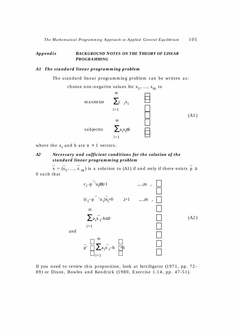
The Mathematical Programming Approach to Applied General Equilibrium 105
Appendix BACKGROUND NOTES ON THE THEORY OF LINEARPROGRAMMING
A1 The standard linear programming problem
The standard linear programming problem can be written as:
choose non-negative values for x1, ..., xm to
maximize Σ
i=1
m
c ixi
subjectto Σi=1
m
aixi≤b
(A1)
where the ai and b are n × 1 vectors.
A2 Necessary and sufficient conditions for the solution of thestandard linear programming problem
x_ = (x
_
1, ..., x_ m) is a solution to (A1) if and only if there exists p
_ ≥
0 such that
ci–p
_′ai≤0,i=1 ,...,m ,
(ci–p_
′ai)x_
i=0 ,i=1 ,...,m ,
Σi=1
m
aix_
i–b≤0
and
p_′
Σ
i=1
m
aix_
i–b =0.
(A2)
If you need to review this proposition, look at Intriligator (1971, pp. 72-89) or Dixon, Bowles and Kendrick (1980, Exercise 1.14, pp. 47-51).
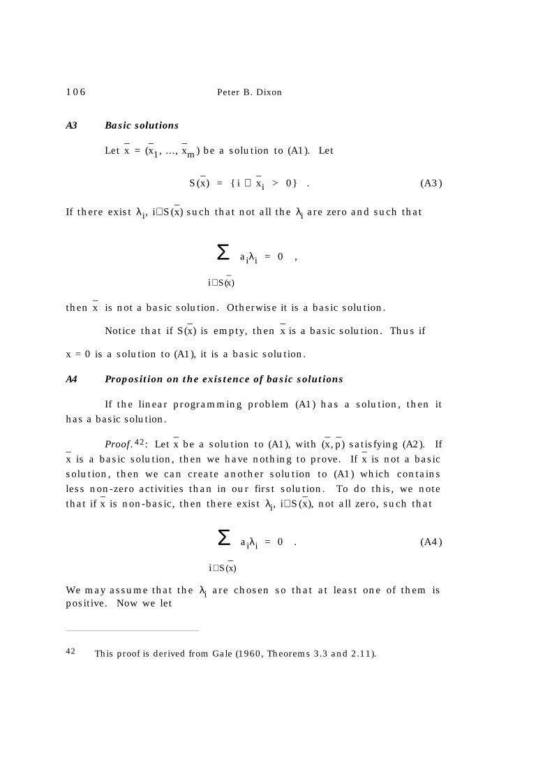
106 Peter B. Dixon
A3 Basic solutions
Let x_ = (x
_
1, ..., x_
m) be a solution to (A1). Let
S(x_) = { i x
_
i > 0} . (A3)
If there exist λi, i∈S(x_) such that not all the λi are zero and such that
Σi∈S(x
_)
aiλi = 0 ,
then x_ is not a basic solution. Otherwise it is a basic solution.
Notice that if S(x_) is empty, then x
_ is a basic solution. Thus if
x = 0 is a solution to (A1), it is a basic solution.
A4 Proposition on the existence of basic solutions
If the linear programming problem (A1) has a solution, then it
has a basic solution.
Proof.42: Let x_ be a solution to (A1), with (x
_,p_) satisfying (A2). If
x_ is a basic solution, then we have nothing to prove. If x
_ is not a basic
solution, then we can create another solution to (A1) which contains
less non-zero activities than in our first solution. To do this, we note
that if x_ is non-basic, then there exist λi, i∈S(x
_), not all zero, such that
Σi∈S(x
_)
aiλi = 0 . (A4)
We may assume that the λi are chosen so that at least one of them ispositive. Now we let
42 This proof is derived from Gale (1960, Theorems 3.3 and 2.11).
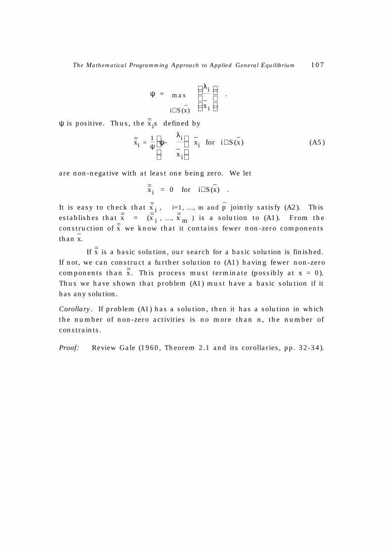
The Mathematical Programming Approach to Applied General Equilibrium 107
ψ = max
i∈S(x_)
λi
x_
i
.
ψ is positive. Thus, the x=is defined by
x=i = 1ψ
ψ–
λi
x_
i
x_
i for i∈S(x_) (A5)
are non-negative with at least one being zero. We let
x=i = 0 for i∉S(x_) .
It is easy to check that x=i , i=1, ..., m and p_ jointly satisfy (A2). This
establishes that x= = (x=i , ..., x=
m ) is a solution to (A1). From the
construction of x= we know that it contains fewer non-zero components
than x_.
If x= is a basic solution, our search for a basic solution is finished.
If not, we can construct a further solution to (A1) having fewer non-zero
components than x=. This process must terminate (possibly at x = 0).
Thus we have shown that problem (A1) must have a basic solution if it
has any solution.
Corollary. If problem (A1) has a solution, then it has a solution in which
the number of non-zero activities is no more than n, the number of
constraints.
Proof: Review Gale (1960, Theorem 2.1 and its corollaries, pp. 32-34).