elg3175 introduction to communication systems fourier ...damours/courses/elg_3175/lec4.pdf ·...
TRANSCRIPT
Fourier transform, Parseval’s theoren, Autocorrelation and Spectral Densities
ELG3175 Introduction to Communication Systems
Fourier Transform of a Periodic Signal
Lecture 4
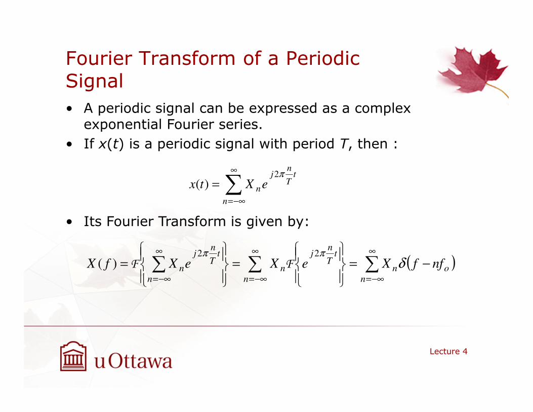
• A periodic signal can be expressed as a complexexponential Fourier series.
• If x(t) is a periodic signal with period T, then :
• Its Fourier Transform is given by:
∑∞
−∞=
=n
tT
nj
neXtxπ2
)(
( )∑∑∑∞
−∞=
∞
−∞=
∞
−∞=
−=
=
=n
onn
tT
nj
nn
tT
nj
n nffXeXeXfX δππ 22
)( FF

Example
Lecture 4
x(t)
0.25 0.5 0.75 t
A
-A
… …
( )∑
∑∑
∞
−∞=
∞
−∞=
∞
−∞=
−
−=
−==
odd is
odd is
4
odd is
4
22
)(
22)(
nn
nn
ntj
nn
ntj
nfn
AjfX
en
Aje
nj
Atx
δπ
ππππ
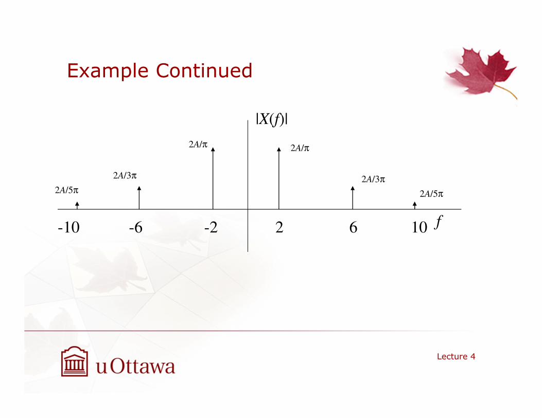
Example Continued
Lecture 4
|X(f)|
f-10 -6 -2 2 6 10
2A/π
2A/3π
2A/5π
2A/π
2A/3π
2A/5π
Energy of a periodic signal
Lecture 4
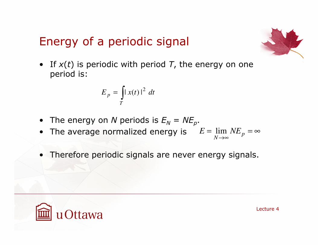
• If x(t) is periodic with period T, the energy on one period is:
• The energy on N periods is EN = NEp.
• The average normalized energy is
• Therefore periodic signals are never energy signals.
∫=
T
p dttxE2
|)(|
∞==∞→
pN
NEE lim
Average normalized power of periodic signals
Lecture 4
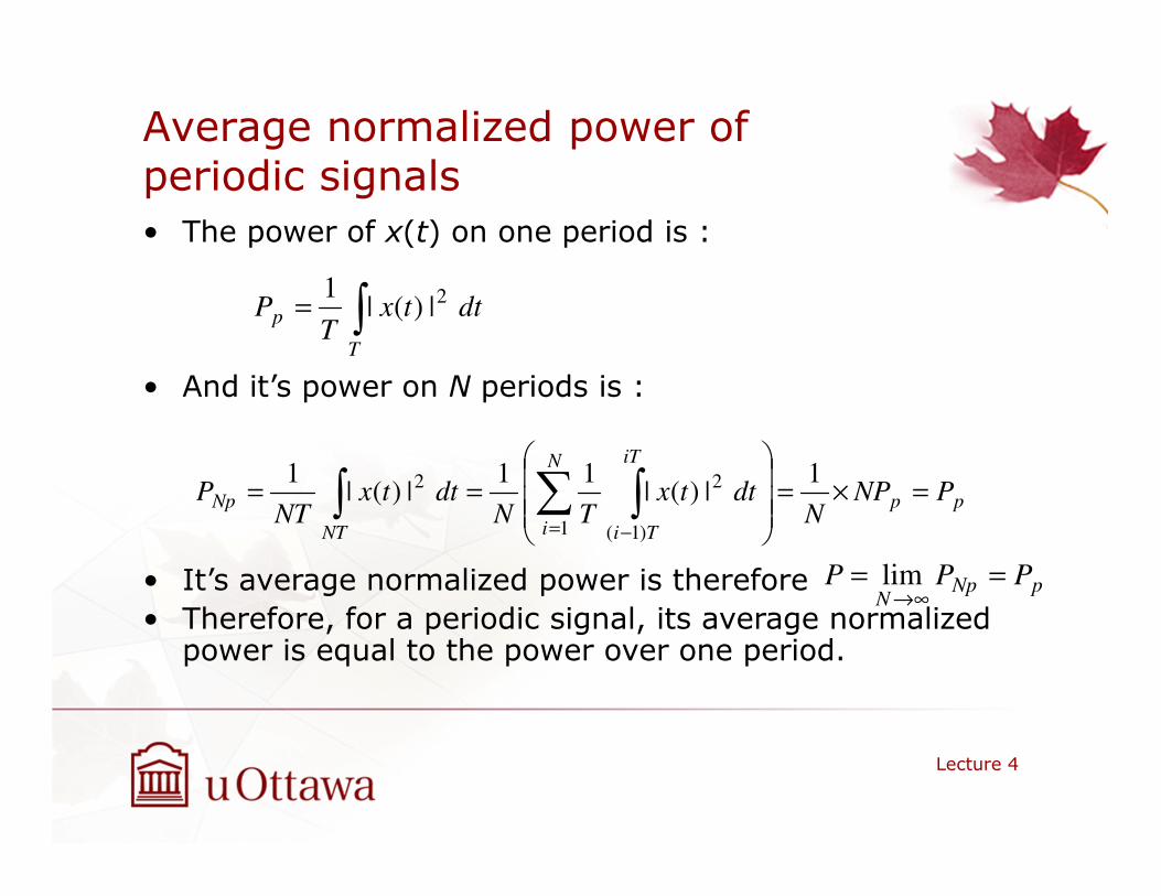
• The power of x(t) on one period is :
• And it’s power on N periods is :
• It’s average normalized power is therefore
• Therefore, for a periodic signal, its average normalizedpower is equal to the power over one period.
∫=
T
p dttxT
P2
|)(|1
pp
N
i
iT
TiNT
Np PNPN
dttxTN
dttxNT
P =×=
== ∑ ∫∫
= −
1|)(|
11|)(|
1
1 )1(
22
pNpN
PPP ==∞→
lim

Hermetian symmetry of Fourier Transform when x(t) is real
Lecture 4
)(
)(
)(
)(
)()(
)(2
2
2*
*
2*
fX
dtetx
dtetx
dtetx
dtetxfX
tfj
ftj
ftj
ftj
−=
=
=
=
=
∫
∫
∫
∫
∞
∞−
−−
∞
∞−
∞
∞−
∞
∞−
−
π
π
π
π
Parseval’s Theorem
Lecture 4
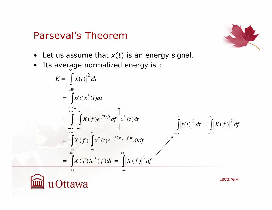
• Let us assume that x(t) is an energy signal.
• Its average normalized energy is :
∫∞
∞−
= dttxE2
)(
∫∫
∫ ∫
∫ ∫
∫
∞
∞−
∞
∞−
∞
∞−
∞
∞−
−−
∞
∞−
∞
∞−
∞
∞−
==
=
=
=
dffXdffXfX
dfdtetxfX
dttxdfefX
dttxtx
tfj
ftj
2*
)(2*
*2
*
)()()(
)()(
)()(
)()(
π
π
∫∫∞
∞−
∞
∞−
= dffXdttx22
)()(
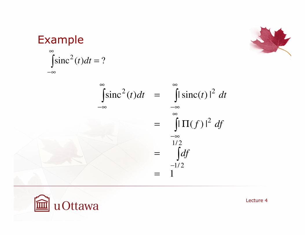
Example
Lecture 4
?)(sinc2 =∫
∞
∞−
dtt
1
|)(|
|)(sinc|)(sinc
2/1
2/1
2
22
=
=
Π=
=
∫
∫
∫∫
−
∞
∞−
∞
∞−
∞
∞−
df
dff
dttdtt
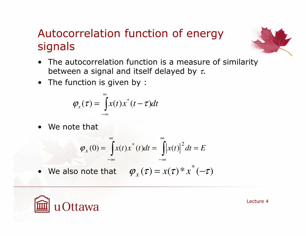
Autocorrelation function of energy signals
Lecture 4
• The autocorrelation function is a measure of similaritybetween a signal and itself delayed by τ.
• The function is given by :
• We note that
• We also note that
dttxtxx ∫∞
∞−
−= )()()(* ττϕ
Edttxdttxtxx === ∫∫∞
∞−
∞
∞−
2*)()()()0(ϕ
)(*)()(* τττϕ −= xxx
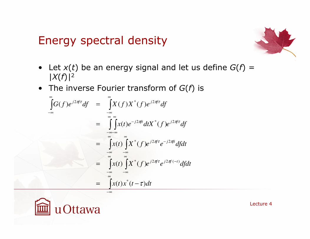
Energy spectral density
• Let x(t) be an energy signal and let us define G(f) = |X(f)|2
• The inverse Fourier transform of G(f) is
Lecture 4
∫
∫ ∫
∫ ∫
∫ ∫
∫∫
∞
∞−
∞
∞−
−∞
∞−
∞
∞−
−∞
∞−
∞
∞−
∞
∞−
−
∞
∞−
∞
∞−
−=
=
=
=
=
dttxtx
dfdteefXtx
dfdteefXtx
dfefdtXetx
dfefXfXdfefG
tfjfj
ftjfj
fjftj
fjfj
)()(
)()(
)()(
)()(
)()()(
*
)(22*
22*
2*2
2*2
τ
πτπ
πτπ
τππ
τπτπ
Energy spectral density
• The energy spectral density G(f) = F{ϕ(τ)}.
• Example
– Find the autocorrelation function of Π(t).
Lecture 4
Energy spectral density of output of LTI system
• If an energy signal with ESD Gx(f) is input to an LTI system with impulse response H(f), then the output, y(t), is also an energy signal with ESD Gy(f) = Gx(f)|H(f)|
2.
Lecture 4
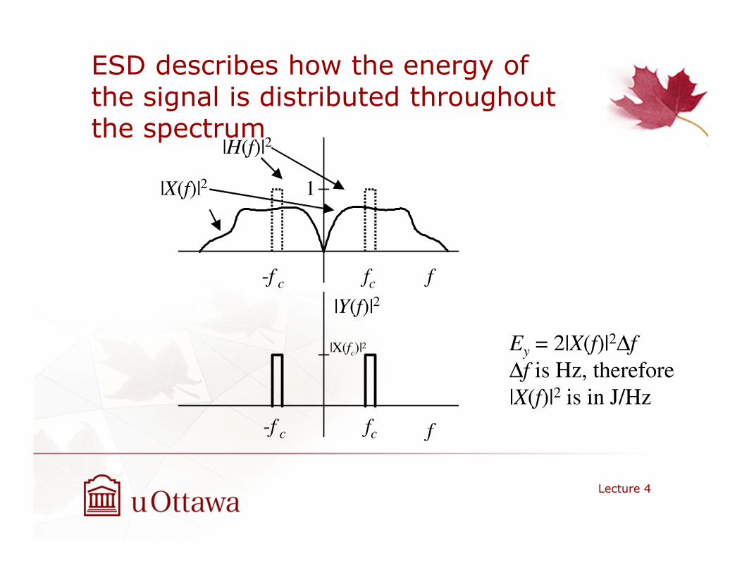
ESD describes how the energy of the signal is distributed throughout the spectrum
Lecture 4
f
|X(f)|2
f
|H(f)|2
|Y(f)|2
-f c fc
-f c fc
1
|X(fc)|2 Ey = 2|X(f)|2∆f
∆f is Hz, therefore
|X(f)|2 is in J/Hz

Autocorrelation Function of Power Signals
• We denote the autocorrelation of power signals as Rx(τ).
• Keeping in mind that for the energy signal autocorrelation, ϕ(0)=Ex, then for the power signal autocorrelation function Rx(0) should equal Px.
• Therefore
Lecture 4
∫−
∞→−=
T
TT
x dttxtxT
R )()(2
1lim)(
* ττ
Power Spectral Density
• Power signals can be described by their PSD.
• If x(t) is a power signal, then its PSD is denoted as Sx(f), where Sx(f) = F{Rx(τ)}.
• The PSD describes how the signal’s power is distributed throughout its spectrum.
• If x(t) is a power signal and is input to an LTI system, then the output, y(t), is also a power signal with PSD Sy(f) = Sx(f)|H(f)|
2.
Lecture 4