Eliminating the observer effect:

Shadow removal in orthomosaics of the road network

Supannee Tanathong*,†, William A. P. Smith* and Stephen Remde†

*Department of Computer Science, University of York, UK†Gaist Solutions Ltd, UK

william.smith@york.ac.uk, {supannee.tanathong,stephen.remde}@gaist.co.uk

Abstract

High resolution images of the road surface can be ob-

tained cheaply and quickly by driving a vehicle around the

road network equipped with a camera oriented towards the

road surface. If camera calibration information is avail-

able and accurate estimates of the camera pose can be made

then the images can be stitched into an orthomosaic (i.e. a

mosaiced image approximating an orthographic view) pro-

viding a virtual top down view of the road network. How-

ever, the vehicle capturing the images changes the scene:

it casts a shadow onto the road surface that is sometimes

visible in the captured images. This causes large artefacts

in the stitched orthomosaic. In this paper, we propose a

model-based solution to this problem. We capture a 3D

model of the vehicle, transform it to a canonical pose and

use it in conjunction with a model of sun geometry to pre-

dict shadow masks by ray casting. Shadow masks are pre-

computed, stored in a look up table and used to generate

per-pixel weights for stitching. We integrate this approach

into a pipeline for pose estimation and gradient domain

stitching that we show is capable of producing shadow-free,

high quality orthomosaics from uncontrolled, real world

datasets.

1. Introduction

High quality, high resolution orthographic images of the

road network are useful for many applications including

mapping, road condition surveying, path planning and tex-

turing of 3D city models. While such images can be ob-

tained by satellite or airborne vehicle, this is expensive,

only possible on cloudless days and resolution and image

quality are limited by the distance of the camera from the

road surface. On the other hand, a road vehicle equipped

with a camera oriented towards the road surface can obtain

very high resolution images of the road surface quickly, at

much lower cost and higher resolution whilst still working

Figure 1. Motivation: when a street level image sequence (top) is

stitched into an orthomosaic (bottom), shadows cast by the capture

vehicle cause artefacts in the stitched result (zoom shows example

of corresponding regions in input and orthomosaic).

on cloudy days. Such images contain perspective distortion

and must therefore be transformed, aligned and stitched in

order to produce a seamless, top down orthomosaic.

However, the drawback of street-level capture is the ob-

server effect - namely that by observing the road scene, we

change it. Specifically, the capture vehicle casts a shadow

onto the road surface that moves as the vehicle moves. If the

captured images are stitched together, the repeated shadow

262

pattern causes severe artefacts in the final orthomosaic. We

show an example in Fig. 1. The zoomed region highlights

an obvious artefacts caused by the shadow of the camera

rig on the capture vehicle. The sawtooth pattern running

through the middle of the image is also a shadow artefact

caused by the shadow from the bonnet of the vehicle.

In this paper, we propose a model-based solution to elim-

inate the observer effect. Note that we do not seek to re-

move all shadows from an image (as is usually the case in

shadow removal). Instead, we only wish to mask shadows

that were created by the process of observing the scene. We

construct an accurate 3D model of the capture vehicle in

canonical pose and registered with the camera used to cap-

ture the road surface. From this model we can compute ac-

curate shadow masks by ray casting and modelling sun ge-

ometry. These shadow masks are transformed to per-pixel

weights used in image stitching that remove artefacts caused

by shadow boundaries. We incorporate this model-based

shadow removal into an orthomosaic pipeline comprising a

lightweight process for estimating camera pose and a gradi-

ent domain stitching procedure. We evaluate our method on

largescale, real world datasets.

2. Related work

City-scale 3D modelling [14] and building orthomosaics

from street-level imagery [3] has been widely studied but, to

our knowledge, the observer effect caused by cast shadows

has never before been addressed.

Images of the road surface can only be captured out-

doors with little or no control over illumination. Thus, shad-

ows are inevitable in the captured images. Although shad-

ows are useful for estimating object shapes [1, 13] and ge-

ometry of the environment and locating the sources of il-

lumination [12], they complicate the interpretation of the

scene. There are many studies that deal with detecting and

removing shadows. Shadow detection approaches exploit

the information extracted from the image content to sepa-

rate shadow from non-shadow regions including colour and

illumination [5], edges or boundary [4] and textures [9]. A

recent study from Khan et al. [8] shows that learned fea-

tures from convolutional neural networks can be used for

generating shadow masks.

Those aforementioned techniques detect and/or remove

shadows that are present in the scene regardless of their

source. In this work, we wish to eliminate only shadows

generated by the observer as these artefacts are not origi-

nally present in the environment. Cast shadows are created

by objects occluding the path from light source to surface.

This work assumes the sun to be the only source of illumi-

nation and the vehicle and attached camera frame are the

only occluding object of interest.

In virtual reality and photo realistic rendering, the effects

of illumination on the appearance of a scene are widely

studied. For example, Sato et al. [12] analyse an illumi-

nation distribution of a scene when an object of a defined

shape casts a shadow in the scene. For outdoor scene, il-

lumination depends on two key elements: sun and weather.

While the position of the sun can be estimated given the

geolocation of the observer and observing time, weather is

rather difficult to predict. Thus, a number of works (e.g.

[6, 7]) model illumination from these two factors discard

the weather condition by assuming clear sky environment.

With this assumption, shadows can be derived from the sun

direction or vice versa. Abrams et al. [1] uses the sun direc-

tion to find the geometric constraints, referred to as episolar

constraints, between the pixels that cast shadows onto oth-

ers and the shadow pixels. By taking an advantage of mul-

tiview image collections, Hauagge et al. [6] begin by recon-

structing geometry of the scene and determine illumination

of images from their local visibility. The sun direction is

estimated by comparing the obtained illumination with one

derived from the sun-sky model. Similarly, Wehrwein et

al. [15] reconstruct 3D model of the scene and analyse il-

lumination within and across images to detect shadows and

further derive the sun direction. In this work, we exploit the

known relationship between the sun direction and shadows

to obtain cast shadows. Given that the acquisition time and

the geolocation of the observer are known, we can deter-

mine the sun direction using [11].

Although our goal is to produce shadow-free orthomo-

saics of the road network, we do not need to modify the

image content to remove shadows. This is because, for our

system, images are captured as a sequence i.e. the same part

of the road surface might have a shadow cast in one image

but be free of shadow in other images. Hence, we only need

to locate shadow free observations of each part of the road

surface in at least one image.

3. Pose estimation

The first stage of our process is to compute an accurate

pose (orientation and position) for the camera in every cap-

tured image. The pose needs to be sufficiently accurate that,

when images are later projected to the ground plane, over-

lapping images have at least pixel-accurate alignment. Oth-

erwise, there will be misalignment artefacts in the generated

orthomosaic images.

We approach the pose estimation problem as a restricted

version of structure-from-motion (SFM). However, previ-

ous approaches for SFM are not applicable in this setting

for two reasons. First, images in which the scene is primar-

ily the road surface are largely planar. This is a degenerate

case for estimating a fundamental matrix and subsequently

reconstructing 3D scene points. Second, the number of 3D

scene points matched between images and reconstructed by

the SFM process is much larger than the number of pose

parameters to be estimated. This means that SFM does

263

2Dmapcoordinatesystem Cameracoordinatesystem

x

y

xy

z (towards !

north)

Figure 2. The camera-centred coordinate systems.

not scale well to very large problems. Similarly, methods

based on Simultaneous Localisation and Mapping (SLAM)

are not applicable. They require high frame rates in order to

robustly track feature points over time. Sampling images at

this frequency is simply not feasible when we wish to build

orthomosaics of thousands of kilometres of road.

We propose an alternative that addresses the drawbacks

of using SFM or SLAM for our problem. Our approach as-

sumes that the scene being viewed is locally planar. This

allows us to relate images that are close together in the se-

quence by a planar homography. We exploit the temporal

constraints that arise from knowing the images come from

an ordered motion sequence by only finding feature matches

between pairs of images that are close together in the se-

quence. We only compute pairwise matches between image

features and do not reconstruct the 3D world position of

image features. This vastly reduces the complexity of the

optimisation problem that we need to solve. The number of

unknowns is simply 6N for an N image sequence.

3.1. Motion model

We refer to the camera mounted on the capture vehicle

as the “carriageway camera”. We represent the pose of the

carriageway camera in each image by a rotation matrix and

translation vector. The pose associated with the ith captured

image is represented by the rotation matrix Ri ∈ SO(3)and the translation vector ti ∈ R

3, with i ∈ [1..N ]. The

position in world coordinates of a camera can be computed

from its pose as ci = −RTi ti.

A world point is represented by coordinates w =[u v w]T , where (u, v) is a 2D UTM coordinate represent-

ing position on the w = 0 ground plane and w is altitude

above sea level. Each camera has a standard right handed

coordinate system with the optical axis aligned with the waxis. A world point in the coordinate system of the ith cam-

era is given by wi = Riw + ti.

It is convenient to represent the rotation as a composi-

tion of four rotation matrices, one of which is fixed. The

fixed one aligns the world w axis with the optical axis of

the camera in canonical pose: Rw2c = Rx(90◦). We model

vehicle orientation by three angles. We choose this repre-

sentation because the vehicle motion model leads to con-

straints that can be expressed naturally in terms of these an-

gles. First, the bearing (yaw) of the vehicle is modelled by

rotation Ry(α). Next, we account for the inclination of the

camera towards the road surface with pitch Rx(β). Finally,

we model side-to-side roll with rotation Rz(γ). The overall

rotation as a function of these three angles is given by:

R(α, β, γ) = Rz(γ)Rx(β)Ry(α)Rw2c. (1)

Hence, the rotation of the ith camera depends upon the es-

timate of the three angles for that camera:

Ri = R(αi, βi, γi). (2)

We assume that each image is labelled with an approximate

geotag, (uGPSi , vGPS

i ), providing an approximate position for

the camera in the ith image in world coordinates. In prac-

tice, this geotag is provided by GPS augmented by wheel

tick odometry. A visualisation of the camera coordinate sys-

tem and rotation angles can be seen in Fig. 2 and the vehicle

in canonical world coordinates in Fig. 4.

3.2. Initialisation

We rely on GPS and an initial estimate of the cam-

era height above the road surface to initialise the location

of each camera: ciniti = [uGPS

i vGPSi W calib]T , where

(uGPSi , vGPS

i ) is the GPS estimate of the ground plane po-

sition of the ith camera and W calib is the measured height of

the camera above the road surface in metres. This need only

be a rough estimate as the value is subsequently refined.

To initialise rotation, we compute the yaw angle from

the GPS bearing. First, we compute a bearing vector using

a central difference approximation:

bi = 0.5

[

uGPSi+1 − uGPS

i−1

vGPSi+1 − vGPS

i−1

]

. (3)

Second, we convert this into a yaw angle estimate:

αiniti = atan2(−bi,1, bi,2). (4)

We initialise the pitch to a measured value for the an-

gle between the camera optical axis and the road surface,

βiniti = βcalib, and the roll to zero, γinit

i = 0. Again, βcalib,

only need be roughly estimated since it is later refined. We

assume that the intrinsic camera parameter matrix, K, and

any nonlinear distortion parameters are measured as part of

a calibration process.

3.3. Feature Matching and Filtering

Our images come from a sequence. Moreover, by using

GPS we can ensure that images are taken at an approxi-

mately fixed distances between consecutive images. This

means that it is reasonable to choose a constant offset O,

within which we expect images to overlap, i.e. we expect

image i to contain feature matches with images in the range

i−O to i+O. The number of overlapping pairs is therefore

NO −O(O + 1)/2.

264

We begin by extracting SIFT features [10] from all im-

ages in a sequence. The 2D location of each feature is

undistorted using the distortion parameters obtained during

calibration. We then compute greedy matches between fea-

tures in pairs of images that are within the overlap threshold.

We filter these matches for distinctiveness using Lowe’s ra-

tio test [10] with a threshold of 0.6. Even with this filter

applied, the matches will still contain noise that will dis-

rupt the alignment process. Specifically, they may include

matches between features that do not lie on the road plane

(such as buildings or signage) or between dynamically mov-

ing objects (such as other vehicles). If such matches were

retained, they would introduce significant noise into the

pose refinement process. We remove these matches by en-

forcing a constraint that is consistent with a planar scene

(the homography model) and further restricting motion to a

model with only three degrees of freedom.

Since we assume the scene is locally planar, feature

matches can be described by a homography. In other words,

if a feature with 2D image position x ∈ R2 in image i is

matched to a feature with image position x′ ∈ R2 in im-

age j, then we expect there to exist a 3 × 3 matrix H that

satisfies:

s

[

x

1

]

= H

[

x′

1

]

, (5)

where s is an arbitrary scale. We use this homography con-

straint to filter the feature matches. However, for the pur-

poses of filtering, we assume a stricter motion model than

elsewhere in the process. Specifically, we assume that the

vehicle has two degrees of freedom to move in the ground

plane and that its yaw angle may change arbitrarily. How-

ever, we assume that pitch and the height of the camera

above the ground plane are fixed to their measured values

and that roll is zero. This allows us to parameterise a ho-

mography by only three parameters and enables us to ignore

matches that would otherwise be homography consistent

but which would lead to incorrect motion estimates. For ex-

ample, if a planar surface (such as the side of a lorry) is vis-

ible in a pair of images, then features matches between the

two planes would be consistent with a homography model.

However, they would not be consistent with our stricter mo-

tion model and will therefore be removed.

Under this motion model, we can construct a homogra-

phy between a pair of images H(u, v, α) based on the 2D

displacement in the ground plane (u, v) and the change in

the yaw angle α. This homography is constructed as fol-

lows. First, we place the first image in a canonical pose:

R1 = R(0, βcalib, 0), t1 = −R1

00

W calib

.

The homography from the ground plane to this first image

is given by:

H1 = K[

(R1):,1:2 t1]

(6)

We define the pose of the second image relative to the first

image as:

R2(α) = R(α, βcalib, 0), t2(u, v) = −R1

uv

W calib.

Therefore, the homography from the ground plane to the

second image is parameterised by the ground plane dis-

placement and change in yaw angle:

H2(u, v, α) = K[

(R2(α)):,1:2 t2(u, v)]

(7)

Finally, we can define the homography from the first image

to the second image as:

H1→2(u, v, α) = H2(u, v, α)H−1

1 . (8)

Given a set of tentative matches between a pair of images,

we now use the RANSAC algorithm to simultaneously fit

our constrained homography model to the matches and re-

move matches that are outliers under the fitted model. Since

our constrained homography depends on only three param-

eters, two matched points are sufficient to fit a homography.

The fit is obtained by solving a nonlinear least squares op-

timisation problem. The RANSAC algorithm proceeds by

randomly selecting a pair of matches, fitting the homogra-

phy to the matches and then testing the number of inliers

under the fitted homography. We define an inlier as a point

whose symmetrised distance under the estimated homogra-

phy is less than a threshold (we use a value of 20 pixels).

This process is repeated, keeping track of the model esti-

mate that maximised the number of inliers. Once RANSAC

has completed, we have a set of filtered matches between a

pair of images that are consistent with our constrained mo-

tion model. Although the model is overly strict, the use of

a relaxed threshold means that matches survive even when

there is motion due to roll, changes in pitch or changes in

the height of the camera.

3.4. Pose optimisation

We now have initial estimates for the pose of every cam-era and also pairs of matched features between images thatare close together in the sequence. We can now performa largescale nonlinear refinement of the estimated pose ofevery camera. Key to this is the definition of an objectivefunction comprised of a number of terms. The first term,εdata, measures how well matched features align in the im-age plane. We refer to this as our data term:

εdata({Ri, ti}Ni=1) = (9)

N−1∑

i=1

min(O,N−i)∑

j=1

Mij∑

k=1

∥

∥

∥

∥

h

(

H−1i

[

xijk

1

])

− h

(

H−1i+j

[

yijk

1

])∥

∥

∥

∥

2

265

where Mij is the number of matched features between im-

age i and i + j, xijk ∈ R2 is the 2D position of the kth

feature in image i that has a match in image i + j. The 2D

position of the corresponding feature in image i+ j is given

by yijk ∈ R2. Hi is the homography from the ground plane

to the ith image and is given by:

Hi = K[

(Ri):,1:2 ti]

. (10)

The function h : R3 7→ R2 homogenises a 3D point:

h([x, y, z]T ) =

[

x/zy/z

]

. (11)

There are some similarities between (9) and bundle adjust-

ment in classical structure-from-motion. However, there are

some important differences. First, rather than measuring

“reprojection error” in the image plane, we measure error

when image features are projected to the ground plane. Sec-

ond, the objective depends only on the camera poses - we do

not need to estimate any 3D world point positions. The first

difference is important because it encourages exactly what

we ultimately want: namely, that corresponding image po-

sitions should align in the final orthomosaic. The second

difference is important because it vastly reduces the com-

plexity of the problem and makes it viable to process very

large sets of images.

To solve (9), we initialise using the process described

above and then optimise using nonlinear least squares.

Specifically, we use the Levenberg-Marquardt algorithm

with an implementation that exploits the sparsity of the Ja-

cobian matrix to improve efficiency. Moreover, we include

some additional terms (described in the next section) to

softly enforce additional prior constraints on the problem.

3.5. Priors

Since we expect the vehicle’s orientation with respect to

the road surface to remain approximately constant, we can

impose priors on two of the angles. First, we expect side-

to-side “roll” to be small. In general, only being non-zero

when the vehicle is cornering. Hence, our first prior simply

penalises the variance of the roll angle estimates from zero:

εroll({Ri, ti}Ni=1) =

N∑

i=1

γ2i . (12)

The second angular prior penalises variance in the angle be-

tween the camera optical axis and the road plane, i.e. the

pitch angle:

εpitch({Ri, ti}Ni=1) =

N∑

i=1

(

βi −1

N

N∑

i=1

βi

)2

. (13)

Mul$viewimages

Carriagewaycameraimage

Figure 3. Left: Subset of the multiview images used to reconstruct

the capture vehicle model. Right: image from the carriageway

camera also used in the reconstruction.

Next, we penalise variance in the estimated height of the

camera above the road surface since we expect this to re-

main relatively constant:

εheight({Ri, ti}Ni=1) =

N∑

i=1

(

ci,3 −1

N

N∑

i=1

ci,3

)2

. (14)

Finally, we encourage the estimated position of the camera

in each image to remain close to that provided by the GPS

estimate:

εGPS({Ri, ti}Ni=1) =

N∑

i=1

(

ci − ciniti

)2. (15)

The hybrid objective that we ultimately optimise is a

weighted sum of the data term and all priors.

4. Model-based shadow removal

The process in the previous section provides us with ac-

curate estimates of the camera pose in world coordinates for

each image in a captured sequence. We now show how to

use a 3D model of the capture vehicle in order to predict

shadow masks. These are used in the subsequent section

during image stitching.

4.1. Model acquisition

We begin by using an existing structure-from-motion

plus multiview stereo pipeline [2] to acquire a detailed 3D

model of the capture vehicle and the ground plane on which

it stands. To do so, we capture 300 images of the vehi-

cle from a range of viewpoints and, to increase the number

of salient features for matching, we place markers on the

ground and around the vehicle. Sample images are shown

in Fig. 3, left. Crucially, the image set includes an image

captured by the carriageway camera on the vehicle (Fig. 3,

right). We include this image in the reconstruction and in

so doing establish correspondence between the carriageway

camera and the 3D model. This later enables us to predict

how the shadow of the van will appear from the perspec-

tive of this camera. The output of this process is a 3D mesh

266

u / East

v / North

w / Up

Figure 4. The captured 3D model in canonical pose relative to the

world coordinate system.

model (Fig. 4) in an arbitrary coordinate system and a cam-

era pose for the carriageway camera relative to this model.

4.2. Model normalisation

We now transform the model into a canonical pose such

that the carriageway camera has centre [0 0 W calib]T and

the u-v projection of its view vector is parallel to the vaxis (i.e. the vehicle points North in the world coordi-

nate system). This is done by combining three transfor-

mations. First, we find the ground plane in the model by

using RANSAC to fit a plane to the mesh vertices. The fit-

ted plane is visualised in blue in Fig. 4. We apply a rotation

and translation to bring this plane into alignment with the

w = 0 plane. Second, we apply a translation in the u-vplane to bring the camera’s centre to the origin. Third, we

project the camera view vector to the ground plane, com-

pute the angle made with the v axis and apply a rotation by

this angle about the w axis. This leaves the model in the

desired canonical pose as shown in Fig. 4.

4.3. Shadow prediction

We compute shadow maps in the ground plane given a

sun direction in the form of a unit vector s ∈ R3, ‖s‖ = 1

relative to the vehicle model in canonical pose (see next sec-

tion for how this is computed). To do so, we first undistort

the coordinates of all pixels in the carriageway camera be-

fore projecting these to the ground plane via the homogra-

phy H1 given in (6). We then project the vertices of the

vehicle model onto the ground plane along direction s. To

determine whether a pixel is shadowed, we simply need to

check whether it lies inside any of the projected triangles

from the model via a point-in-polygon test. This ray casting

process gives us a binary label for each pixel in an image

from the carriageway camera’s perspective. We show a vi-

sualisation of this process in Fig. 5.

Figure 5. Shadow prediction. Ground plane projection of carriage-

way camera image shown in red. Ray cast shadow map of vehicle

model shown in green.

4.4. Sun geometry

The final step is to compute the sun direction vector for

an image and to transform it into the coordinate system

of the canonical model. We assume that our images are

timestamped and so we do not need to estimate the sun di-

rection (such as in [6]), we can simply compute it. Since

our camera pose estimates were initialised with GPS posi-

tions, we can assume that the estimated camera centres are

in world coordinates. i.e. they can be converted into lati-

tude/longitude values. From this, we can compute the sun

direction, s ∈ R3, ‖s‖ = 1, using standard formulae (refer

to [11]). Finally, to transform the sun direction into the co-

ordinate system of the canonical model, we apply a rotation

about the vertical axis to factor out the bearing of the vehi-

cle: s = Rz(−α)s, where α is the estimated yaw angle of

the vehicle.

4.5. Shadow maps to weights

Ray casting a shadow map from a high resolution mesh

model is computationally expensive. Hence, in a large-scale

system we may wish to avoid performing this computation

for every frame. We propose to precompute a lookup table

for shadow masks. This need only be two dimensional, for

the two degrees of freedom of s. Moreover, only directions

in the half-hemisphere s2 < 0 ∧ s3 > 0 need be considered

(for all other directions, the van casts no forward shadow

in the ground plane). At stitching time, we compute a sun

direction in the canonical model coordinate system, round

to the nearest lookup table bin and retrieve the associated

shadow map. We combine this with a per-pixel weight map

in which pixels are given a higher weight that are closer to

the camera. We precompute these distances for the canoni-

cal van model and combine them with the shadow mask for

each image, assigning zero weight to shadowed pixels.

5. Gradient domain stitching

The final step in our pipeline is to stitch the images cap-

tured by the carriageway camera into a seamless orthomo-

saic. We do this in tiles both to ensure it is computationally

feasible to stitch very large datasets and also so that large

datasets can be viewed online by only transferring visible

tiles. We perform stitching in the gradient domain to hide

seams that would otherwise be visible due to the camera

267

exposure varying and small errors in the image alignment.

For an M × M tile in the ground plane, we solve for

the vector of intensities a ∈ RM2

such that its gradients

recreate those selected from the “best” original image at

each pixel whilst also matching guide intensities to remove

colour offset indeterminacy. This can be written as a linear

least squares problem:

a∗ = argmina

∥

∥

∥

∥

∥

∥

Dx

Dy

λS

a−

gx

gy

λiguide

∥

∥

∥

∥

∥

∥

2

. (16)

Here Dx,Dy ∈ RM2

×M2

compute finite difference ap-

proximations to the gradient in the horizontal and verti-

cal directions respectively (they are sparse having only two

non-zero entries per row if forward/backward differences

are used). S ∈ {0, 1}K×M2

is a selection matrix that se-

lects K intensities for which guide values are provided.

gx,gy ∈ RM2

are per-pixel gradients selected from the

image whose corresponding pixel had the highest weight.

In practice they are obtained by computing gradients for

each input image and interpolating into these at the position

given by projecting a tile pixel into the image. iguide ∈ RK

contains guide intensity values for K pixels. In practice,

for guide intensities we use the average of all intensities

that were observed for a given tile pixel and choose the Kpixels as a sparse regular grid over the image (specifying

guide values for all pixels causes the stitched image to be

oversmooth and contains seams, equivalent to simply aver-

aging the aligned images). λ controls the influence of the

gradient versus the guide intensity objectives and is set to a

small value. We solve an equation of the form of (16) for

each colour channel for each tile.

The role of the weights is to try to select a gradient for

each pixel that comes from the image most likely to contain

detail. Hence, we use a weight mask that assigns to each

pixel the distance to the ground plane. Pixels with higher

weight are closer and hence imaged at a higher resolution.

These fixed weights are combined with a per-image shadow

mask such that shadowed regions are never selected.

6. Experiments

We acquire a sample dataset by driving a camera-

equipped vehicle along a section of road. The carriageway

camera is pre-calibrated. The initial estimates for the cam-

era height and pitch angle can be taken from the multiview

reconstruction of the vehicle described in Section 4.1. We

use a 50 image sequence and show sample input images in

Fig. 6 (left). The corresponding shadow maps from ray cast-

ing are shown in the middle and the weight maps used for

stitching on the right. The orthomosaic produced by gradi-

ent domain stitching is shown in Fig. 7. Note that these im-

ages are in fact made up of multiple tiles though the seams

Figure 6. Orthomosaic inputs. Left: images captured by our cam-

era equipped vehicle in which the shadow of the camera rig is vis-

ible in the bottom right of the image. Middle: their corresponding

shadow masks determined based on the the sun direction and the

bearing direction of the vehicle. Right: stitching weights (darker

equals lower weight, black equals zero weight).

are not visible. The green background indicates regions that

were not observed in any image. The image on the left of

Fig. 7 is the result of stitching without using shadow masks

in which an artefact of a repeated pattern of the shadow is

visible which was not originally present in the real envi-

ronment. Using the shadow masks, the orthomosaic on the

right shows that shadows are completely removed while still

maintaining all the details of the captured images. Fig. 8

shows a zoomed segment of the two results.

7. Conclusions

In this paper we have presented a model-based method

for predicting the location of shadows in images of the road

network and a pipeline to stitch shadow free, seamless or-

thomosaics from street level images. The approach success-

fully removes the observer effect and leads to high quality

virtual top view images. There are many in ways in which

this work could be extended in future. First, in the current

implementation we set the stitching weight to zero in the

entire shadow region. In fact, gradient domain stitching is

only disrupted by the large gradients introduced at shadow

boundaries. So, the interior of the shadow could be given

positive weight, increasing the image data available. Sec-

ond, the motion and road geometry model make a planarity

assumption that is clearly violated in the real world. There

may be an alternative lying between SFM (which computes

an unrestricted 3D point cloud model) and a planarity as-

sumption. For example, we could assume that the road sur-

face can be locally approximated by a parametric patch and

solve for the local parameters during pose estimation.

Acknowledgements

This work was supported by Innovate UK grant

KTP009627.

268

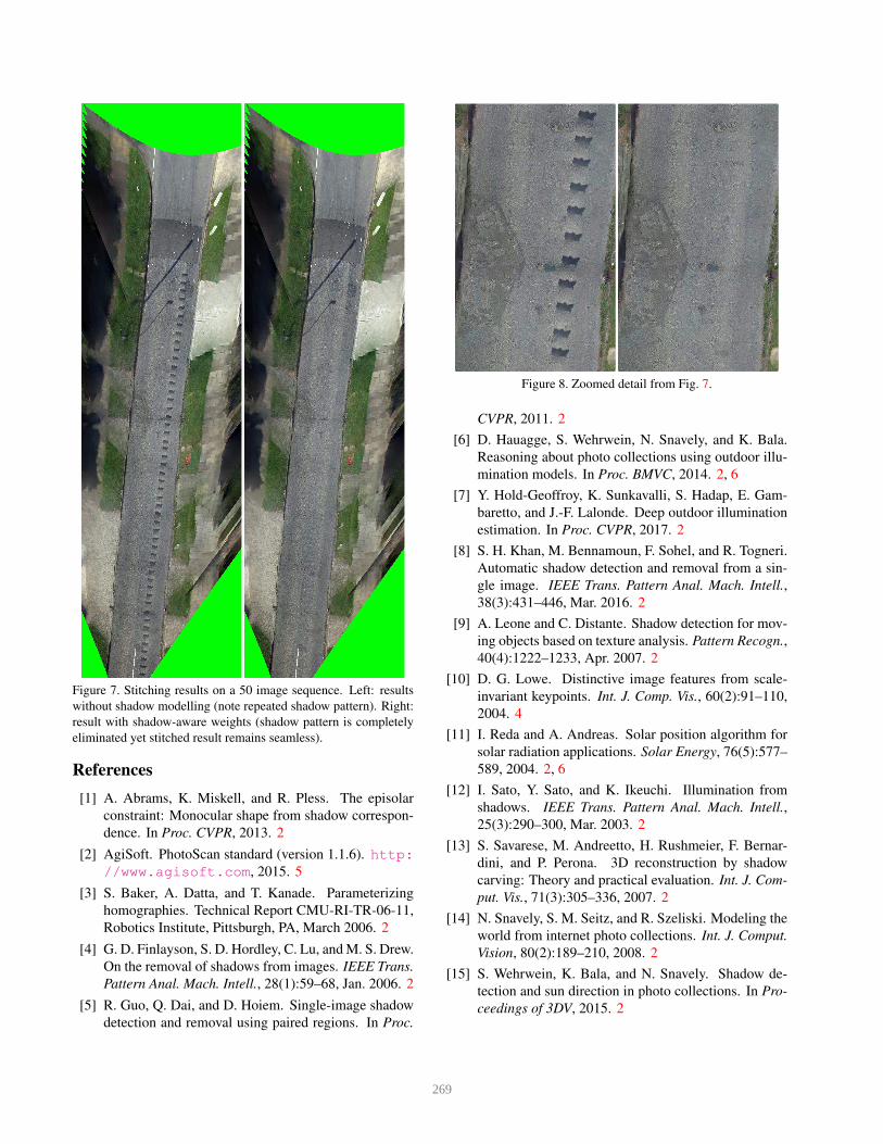
Figure 7. Stitching results on a 50 image sequence. Left: results

without shadow modelling (note repeated shadow pattern). Right:

result with shadow-aware weights (shadow pattern is completely

eliminated yet stitched result remains seamless).

References

[1] A. Abrams, K. Miskell, and R. Pless. The episolar

constraint: Monocular shape from shadow correspon-

dence. In Proc. CVPR, 2013. 2

[2] AgiSoft. PhotoScan standard (version 1.1.6). http:

//www.agisoft.com, 2015. 5

[3] S. Baker, A. Datta, and T. Kanade. Parameterizing

homographies. Technical Report CMU-RI-TR-06-11,

Robotics Institute, Pittsburgh, PA, March 2006. 2

[4] G. D. Finlayson, S. D. Hordley, C. Lu, and M. S. Drew.

On the removal of shadows from images. IEEE Trans.

Pattern Anal. Mach. Intell., 28(1):59–68, Jan. 2006. 2

[5] R. Guo, Q. Dai, and D. Hoiem. Single-image shadow

detection and removal using paired regions. In Proc.

Figure 8. Zoomed detail from Fig. 7.

CVPR, 2011. 2

[6] D. Hauagge, S. Wehrwein, N. Snavely, and K. Bala.

Reasoning about photo collections using outdoor illu-

mination models. In Proc. BMVC, 2014. 2, 6

[7] Y. Hold-Geoffroy, K. Sunkavalli, S. Hadap, E. Gam-

baretto, and J.-F. Lalonde. Deep outdoor illumination

estimation. In Proc. CVPR, 2017. 2

[8] S. H. Khan, M. Bennamoun, F. Sohel, and R. Togneri.

Automatic shadow detection and removal from a sin-

gle image. IEEE Trans. Pattern Anal. Mach. Intell.,

38(3):431–446, Mar. 2016. 2

[9] A. Leone and C. Distante. Shadow detection for mov-

ing objects based on texture analysis. Pattern Recogn.,

40(4):1222–1233, Apr. 2007. 2

[10] D. G. Lowe. Distinctive image features from scale-

invariant keypoints. Int. J. Comp. Vis., 60(2):91–110,

2004. 4

[11] I. Reda and A. Andreas. Solar position algorithm for

solar radiation applications. Solar Energy, 76(5):577–

589, 2004. 2, 6

[12] I. Sato, Y. Sato, and K. Ikeuchi. Illumination from

shadows. IEEE Trans. Pattern Anal. Mach. Intell.,

25(3):290–300, Mar. 2003. 2

[13] S. Savarese, M. Andreetto, H. Rushmeier, F. Bernar-

dini, and P. Perona. 3D reconstruction by shadow

carving: Theory and practical evaluation. Int. J. Com-

put. Vis., 71(3):305–336, 2007. 2

[14] N. Snavely, S. M. Seitz, and R. Szeliski. Modeling the

world from internet photo collections. Int. J. Comput.

Vision, 80(2):189–210, 2008. 2

[15] S. Wehrwein, K. Bala, and N. Snavely. Shadow de-

tection and sun direction in photo collections. In Pro-

ceedings of 3DV, 2015. 2

269