Introduction

Voluntary movements such as reaching and grasping are easy to do, but the complex computations

involved are difficult to explain. Complicated problems of this kind can be simplified by dividing them

into sub-tasks. Most studies implicitly assume a division into two tasks, sensory and motor. This approach

requires the same system to compute both the geometry of the trajectories and the forces needed to

implement them. Explaining how the brain can do these computations with redundant degrees of freedom

has not been addressed in computational motor control. In this paper we take a novel approach to

decomposing the sensory-motor pathway. Instead of assuming a two-stage system, we interpose a third,

or geometric stage, between the sensory and motor stages. This stage computes the geometric aspects of

movement, but not the forces. It receives proprioceptive input about the current state of the system and

visual input related to the current goal. Its output feeds geometric information to the motor stage where it

is used to guide the implementation of movement. The advantage of this approach is that complex

realistic movements with redundant effectors can be relatively easily specified in terms of variables that

are controllable by the motor system, simplifying the task of motor implementation.

We focus on the geometric stage and provide an explicit, gradient based, computational model that

specifies various kinematics aspects of the motion. The model is used to show how difficult problems

such as excess degrees-of-freedom, path under-determination, error correction and constraint satisfaction

can be solved geometrically. The behavior of a seven-degree of freedom arm making reach to grasp

movements in 3D is simulated as an example.

Previous Work

The idea of separating kinematics from dynamics in biological motor control is not without precedents

(Hinton 1984), but it has not been widely used despite experimental data showing that force-independent

1

kinematical representations exist in movement related brain areas (Kalaska et al. 1990). Our motivation

for introducing a separate geometric stage came from the difficulty of solving the problem of under

determinacy inherent in specifying the movements of many jointed limbs (Bernstein 1967). Two

important sources of movement under determinacy are excess degrees of freedom and path redundancy. If

there are more degrees of freedom in the limb than in the space it moves in there are infinitely many

postures corresponding to each hand location and orientation. There are also infinitely many paths to the

same goal, whether or not there are excess degrees of freedom. It remains unknown how the brain

generates the possible solution paths or how it chooses one trajectory from all the possible ones.

Under determined problems are generally solved by optimization. The most common computational

approach has been to consider the problem as analogous to one in classical mechanics. In this

formulation, the trajectory that minimizes an energy-like quantity must be found. This requires integrating

a complicated function along all possible trajectories to find the one that is optimal according to some

pre-set criterion. These integrals generally require that the final posture and the elapsed time be known

prior to movement, making the computations daunting when the tasks are underdetermined. Because of

this, almost all the work has been done with simplified systems having two degrees of freedom and

moving in a plane, i.e. with no excess degrees of freedom. Under very simplified conditions the

minimizing integral equations can be solved, but in most cases they cannot and many numerical

integrations are required to find the minimizing path. Models of this general type such as minimum jerk

(Flash and Hogan 1985), minimum torque (Uno et al. 1989), minimum metabolic energy (Alexander

1997) and minimum variance (Harris and Wolpert 1998) have played a useful role in the study of planar

arm movement. However, explaining current experimental data from realistic-unconstraint arm motions

may require a different computational strategy. The former approaches are particularly unsuited for

finding complex paths, correcting errors on line and satisfying multiple constraints when the arm has

2

redundant degrees of freedom. There is experimental evidence showing that reaching paths remain

invariant under moderate changes in such physical variables as speed and loading (Atkeson and

Hollerbach 1985), (Nishikawa et al. 1999). This suggests that at least in the context of these tasks,

geometry might be a rather important component in guiding the movement.

The Geometric Stage

The geometric stage is a computational module between sensory input and motor output. Its inputs consist

of extrinsic information such as target location and orientation, and an intrinsic description of the current

posture. The target information can come from any sensory system, typically vision. The posture

information comes from somatic sensory feedback or from a feed forward model. The geometric stage

continually outputs a stream of changes in postural variables that brings the hand to the target in the

correct orientation for grasping. Physically implementing these changes in posture is the job of the motor

stage. This means that observed behavior will, in general, be guided by the geometric stage. This is a

critical point because it implies that a model of the geometric stage can predict essential aspects of

observed behavior.

It is not yet known what postural variables are actually controlled by the motor system. Joint angles and

muscle lengths are possibilities. A particular set of joint angles is used in our model only for specificity,

but all the basic principles remain the same if different variables are used. There are two important

features of the geometric stage to keep in mind. First, it computes the geometrical aspects of movement,

but not the forces required to bring these changes about. And second, it specifies movement paths,

independent of the speed of movement. This is analogous to controlling a car where direction is specified

by the steering wheel, while speed is controlled independently by the accelerator and break. The actual

3

forces needed to achieve movement are computed by motor systems in the car. Our current model is

concerned only with the ‘direction’, i.e. path of movement.

We use gradient descent as the differential optimization technique in our model of the geometric stage.

Gradient descent requires a function that maps all the variables that specify posture, e.g. joint angels, to a

positive scalar that decreases as the posture approaches its target value. Various disciplines use different

names for this function such as cost, error, principle and energy function. We will use cost function.

Relatively simple, distance like, measures can be used for the cost function in the geometric stage. The

gradient of the cost function is a vector in joint angle space whose components tell how much to change

each joint angle to get the arm closer to the target position and orientation. We illustrate the gradient

technique using an arm with seven degrees of freedom (dof) that does reach-to-grasp movements in three

dimensions.

The Model: Computing the Gradient

The model deals with two phases of grasping: Transport -- moving the hand to the object. Orientation --

rotating the hand to match the object axis. Therefore, the cost function has to map joint angles to a single

value that combines distance to the target with the difference in orientation between hand and target. We

first describe using gradient descent for transport.

Consider an arm consisting of constant length segments linked end to end by n flexible joints. One end of

the arm is attached to a fixed point in a 3D reference frame and the other end, i.e. the hand, remains

unconnected, Figure 1. Let X, the workspace, be the set of points that can be reached by the hand in 3D

space. Let Q, the configuration space, or specifically here, the joint angle space, be an open subset of .

4

The components of Q are any set of variables, i.e. joint angles, which can specify all arm postures. For

our example we use the Euler angle sequence given in Figure 1 to describe a 7 degree-of-freedom arm.

There is a vector valued kinematics function, that maps Q onto X, i.e. every hand location can be

written as for at least one , and every maps to some .

Where:

Since the arm segment lengths are considered constant, we ignore them in the notation used here. We are

interested in cases were the joint angles are limited to their physiological ranges and , i.e. there are

redundant degrees of freedom. The function for the 7- jointed arm in Figure 1 can be found in the

literature (Benati et al. 1980).

A trajectory in Q is a directed path that connects two postures qinitial and qfinal. The path in X traced by the

hand corresponding to a trajectory in Q is called its image in X. A trajectory in Q that solves the problem

is given by moving along the path:

where is the cost function representing the distance in X between and and dt

is a scalar parameter. The cost is a positive function with a unique global minimum 0,

which occurs at the target point. Using f, can be written explicitly:

5

The gradient of is given by the chain rule:

Next we consider using gradient descent to reduce the difference in orientation between the hand and the

target object. We need to find a single value that decreases with this difference in orientation and is a

function of q and the orientation of the target. Our strategy is to first find the matrix that represents a

rotation that will align the target with the hand. This rotation can then be represented by a single angle

about the principal axis (Altman 1986). This angle can be used in the cost function. The general

scheme is given below.

Solving The Orientation-Matching Problem

Consider three reference frames: one fixed at the shoulder S, one on the hand H, and one on the object O,

Figure 2. The relative orientation of these frames can be represented with orthogonal rotation matrices:

for the rotation from shoulder to hand, from shoulder to object, and , from object to

shoulder to hand, where is the rotation from object to shoulder. Note that depends on the

posture q, while is given as input to the geometric stage. The matrix depends on both the current

posture and the object's orientation and represents the orientation difference we want to reduce.

To get a single value for the orientation difference we use the fact that for any rotation matrix, such as ,

there is a principal axis about which a single rotation has the same effect as the rotation matrix. A

cost function for reaching-to-grasp can be obtained by combining with the distance term derived

above:

6

Where is a parameter that can be adjusted so that arm movement and hand rotation overlap realistically

in time as the arm moves towards the target, and . In our simulations we set the

parameter to a constant so that the transport and orientation errors decrease proportionally. However,

whether these errors change independently or not remains an open question that needs to be addressed

experimentally.

The gradient descent algorithm starts at , takes a small step in the direction of the negative gradient

to a new point This procedure is repeated using successive values of until the value of r

goes to zero, at which point equals , and the hand orientation matches the object’s. In

practice, computation is stopped when r is less than some small tolerance. Ideally the steps should be

infinitesimal, but the gradient is approximated quite well using moderately large steps. An important

feature of the gradient paradigm is that the trajectories obtained in Q provide a complete description of all

arm configurations as movement proceeds from initial to final posture. The actual trajectories generated

by the gradient method depend on the metric of the configuration space. The significance of this

important issue will be addressed later.

An important property of (4) is that r goes to zero if and only if the hand is at the target in the correct

orientation. This enables the system to avoid the problem of local optima that can plague gradient

descent. If the gradient of r goes to zero and r is not zero then a perturbation can be made in the trajectory

and gradient descent continued until r is zero. This is not a trivial feature of the exact form of the cost

function (4). Rather it comes from the fact that distance and orientation difference are geometrical

properties of the system that go to zero only when the reach-to-grasp task is complete.

7

Generalization of the Method

So far we have assumed a Cartesian coordinate system to represent postures, and used a Euclidean metric

(norm or inner product) in this space. These however were only chosen for specificity. We now explore

other possibilities to generalize our formulation, and include multiple movement constraints.

It is possible to use different metrics to automatically encode other aspects of movement within the

gradient-based solution. This is because by definition the gradient of a function depends on the metric

(Appendix A.1) of the parameter space, regardless of the coordinate representation of choice. Thus, if we

change the metric of configuration space, we can change the solution paths selected by the algorithm

(Appendix A.2). By the same principle, we can then approximate desirable paths to comply with different

tasks constraints.

Using a Cartesian (‘flat’) coordinate representation associated to a ‘non-flat’ metric accomplishes the

same as appropriately ‘warping’ the coordinate representation while keeping a Euclidean (‘flat’) metric.

The former interpretation permits us to introduce different metrics to automatically account for multiple

movement constraints or extra-preferences in our solution. The latter allows us to formally approximate

an adequate coordinate representation to define motions that are due to a specific task. This more general

formulation attempts to address the question of how the brain resolves similar tasks under different

constraints. We illustrate both interpretations in what follows.

A Simple Example

Consider the pointing problem in 2D: we want to move the tip of a 2-link planar arm from an initial

configuration to a given target point , but respecting the extra-constraint that the endpoint path

be a straight line.

8

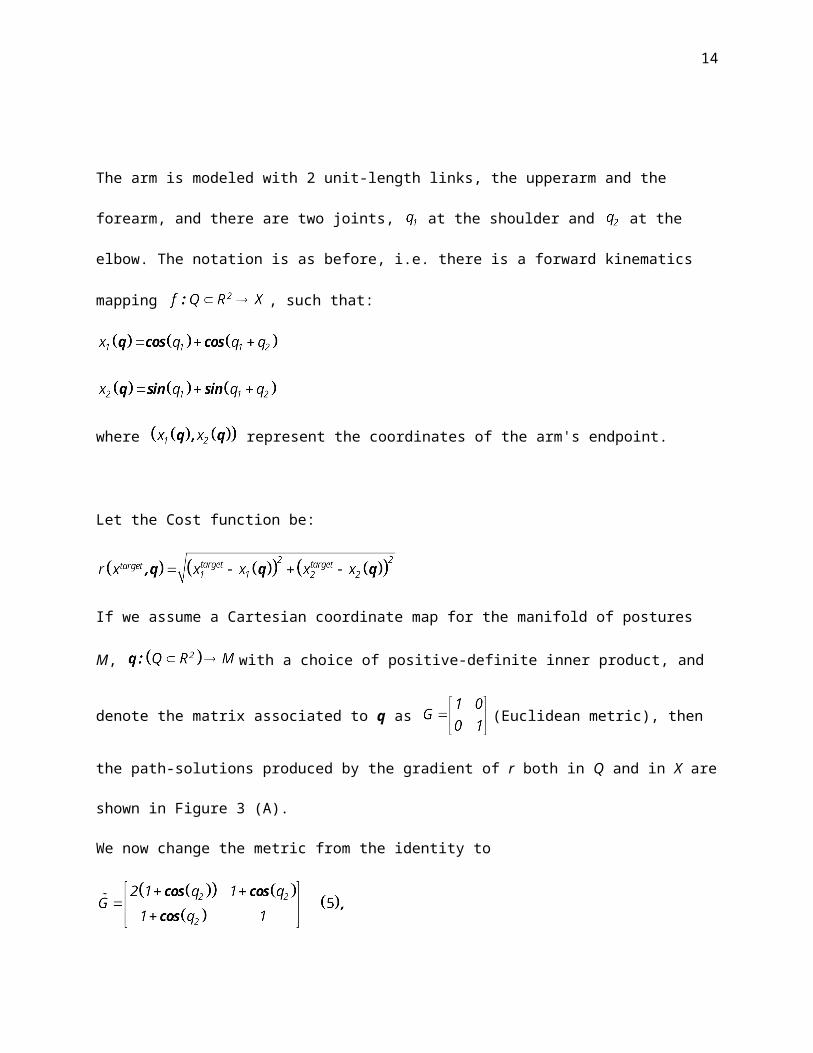
The arm is modeled with 2 unit-length links, the upperarm and the forearm, and there are two joints, at

the shoulder and at the elbow. The notation is as before, i.e. there is a forward kinematics mapping

, such that:

where represent the coordinates of the arm's endpoint.

Let the Cost function be:

If we assume a Cartesian coordinate map for the manifold of postures M, with a choice

of positive-definite inner product, and denote the matrix associated to q as (Euclidean metric),

then the path-solutions produced by the gradient of r both in Q and in X are shown in Figure 3 (A).

We now change the metric from the identity to

keep the Cartesian coordinate map q, and correct the gradient to account for the change of metric:

. This yields the desired straight-line path shown in

Figure 3 (B).

9

Equivalently, following the gradient of r after an adequate coordinate transformation associated to a

Euclidean metric accomplishes the same extra-preference (Appendix A.3):

We use as a different coordinate map (Figure 4), where for some

positive-definite transformation matrix , where:

and the forward kinematics function f maps postures to X using the new -coordinates, .

The same straight-line path in X is achieved with the new -parameterization and old as with the

old q-Cartesian coordinates and the new metric . The coefficients of the new metric due to a change

of coordinates under the old metric can be obtained and yield the same matrix as in (5) (Appendix A.4).

This simple 2D example shows the flexibility this general formulation adds to the method.

In figure 5 we show another instance in which a correction of the metric yields the shortest-distance

paths. Here, the azimuth and elevation angles described by an ideal model (ball-and-socket) of the

glenohumeral joint at the shoulder are corrected to constraint motions to follow greater circle paths on the

unit sphere. Under Euclidean metric, the solution path to the given target is curved, but the same path

computed using the more ‘natural’ metric is a ‘straight line’ on the sphere.

Next, we use the notion of a change in the metric associated to a Cartesian q-coordinate representation to

implement movement constraints for the more complex instance of an arm with 7 dof.

Constraint Satisfaction in Goal-Directed Motions

There are many constraints imposed on arm movements due to task specificity. Some allow us to save

effort by biasing the upperarm to remain closer to its resting posture. Others prevent painful motions by

10

keeping the movement within a subset of the full range of motion at the joints. We treat these constraints

as movement sub-goals and implement them using the properties of the gradient operator described

above.

As before, the general idea is to pre-multiply the gradient by a positive-definite matrix (the metric tensor),

which we denote here by to represent the constraints. This yields a new gradient vector denoted by

guaranteed to still decrease the original cost. This is because is positive-definite, which implies

that when , so the new gradient vector is within of the old . In

addition, if and only if , so all minima of the cost function are still minima, and

no new minima are introduced.

Simulated Constraints: Saving Effort

The upper arm requires more effort to elevate than the more distal arm segments because it is heavier.

Effort can be saved by discriminating against elevating the upper arm away from its resting position and

enhancing movement back towards rest. This can be implemented by changing the metric of Q space. The

matrix C in this case, is diagonal with all diagonal components equal 1.0 except for the one associated

with the elevation angle of the upper arm. The component corresponding to the upper arm is set to some

function, were and are the enhancement and

discrimination factors respectively, , i ranges over all joint angles, and k is a constant that

determines the sharpness of the transition between the and the states. Figure 6 depicts the

trajectories resulting from simulating motions using the gradient method under this constraint. They are

obtained by using:

where

11

and

Simulated Constraints: Moving Comfortably

The limitations on joint angle flexion can also be expressed using a diagonal matrix, but now each

diagonal component is a function that goes to zero when the associated change in joint angle moves it

outside its allowed range and stays at one otherwise. To get such a function we combine a function having

partial derivatives of 1.0 in range and 0.0 out of range multiplied by a direction discriminating function of

the kind used above. An example is:

where and are the limits of joint angle i flexion. Here is set to 1.0 and to 0.0. The arm

elevation and joint angle range constraint can be applied simultaneously by chain-multiplying their

matrices.

Experimental Example

Up to this point, we have presented various simulated examples of how to impose extra-constraints or

preferences in the motion using different metrics. We have also shown in the 2D example how the idea of

12

an adequate change of metric can be applied to obtain a coordinate transformation that under Euclidean

metric yields the desired paths. We now show how to extract this information from experimental human

motion data recorded using the Polhemus Fastrak motion tracking system. The experiment was to match a

given target position and orientation with a hand-held cylinder, starting from the same arm posture, and

moving at a normal pace (6 repetitions). The seven-joint angle paths that reconstruct the position and

orientation sensor paths were obtained (Torres 2001) to compare to the gradient-based solution paths

generated for the corresponding starting posture and target positions and orientations.

The question we address is how to obtain the data paths given the gradient-generated paths computed

under an arbitrarily chosen coordinate representation and metric. What we want is a change of metric that

under the chosen coordinates representation and the gradient-based solution gives the data paths, or

equivalently a coordinate transformation that produces the data paths in a Euclidean space. Thus, given

and , we want a symmetric-positive-definite matrix M1 that transforms X into Y,

, such that (Appendix A.5).

The model-generated paths obtained after changing from the identity matrix to and using

are plotted in figure 7 superimposed on the actual data paths from

the hand sensor. The matrix is computed across the entire data set for each subject. Table 1 lists

for each subject the mean absolute deviations (in radians) for the difference between the data and the

model obtained using .

This experimental example is merely used to illustrate the general method we propose. It should be noted

however, that although we obtain a good fitting, the actual metric tensor we are after should vary as a

function of posture (work in progress). This data set does not provide us with enough sample points to

estimate it, so we have settled for the same matrix for all the postures involved. The key point is that in 1 We impose the symmetric-positive-definite constraint to ensure a coordinate transformation that preserves the properties of a

space with a Euclidean inner-product.

13

our formulation of the solution the coordinate representation used to describe postures becomes

irrelevant. What is important is the knowledge of the metric(s) of the space, a property any system can

learn from experiencing the physical world surrounding it. Furthermore, if we tie this information to the

task the system is resolving, we might be able to say something more about the cost whose new gradient

under Euclidean space assumption and the original coordinates has become

. The cost in question can be recovered by

integration (Shilov 1968). This approach enables us to formulate new experimental questions regarding

important issues arising in realistic motions of an arm with redundant dof.

Behavioral Predictions

The arm trajectories computed by the geometric stage will be reflected in observed behavior if, as we

conjecture, the motor stage implements these trajectories. This means that various features of the

trajectories computed using the gradient paradigm should be comparable to actual arm movements. For

example, simulated orientation-matching motions using this method produce smooth hand paths. They

reflect the dependence of final posture on the starting posture, and show the co-articulation of hand

orientation with arm movement observed in reach-to-grasp movements (Soetching et al. 1995),

(Desmurget et al. 1998). Differences in posture paths, and hand position and orientation paths due to 2

initial postures are shown in Figure 8 (A), (B) and (C) respectively. Simulated paths are superimposed on

the actual paths from one of our subjects.

Paths resulting from movements from a single starting posture to targets located in the same position but

oriented differently are shown in Figure 9. The effect of target orientation on the position hand paths, the

orientation hand paths and the postural paths are shown in Figure 9 (A), (B) and (C) respectively. They

are also superimposed on the motion paths of one subject. A detailed analysis of these experiments will

be presented elsewhere.

14

Error Correction

There are many sources of error that can cause deviations from the desired movement path. An important

task for any real sensory-motor system is to compensate for these errors enabling movement goals to be

reached. An advantage of the gradient method is that some of these errors are automatically corrected at

the geometric stage. We simulate 2 sources of error due to perturbations. Figure 10 (A) illustrates the

hand position paths resulting from perturbations applied in configuration space. At each time step, 2

different levels of random noise are used to affect the incremental directional signal output by the

gradient. Because the geometric stage continually receives input regarding the current posture and visual

goal, the hand moves toward the target irrespective of where the perturbation has put it. The paths are

deformed, but still reach the target.

In Figure 10 (B), we simulate a sudden change in target position during the movement. The model also

handles these kinds of on-line perturbations and achieves the target because it receives visual input related

to the current goal position and orientation at each time step (Prablanc and Martin 1992).

Arbitrary Trajectories

Real hand movements are often complex with many rapid changes in direction. Examples are paths that

avoid obstacles and tasks such as drawing and writing. The gradient method makes it possible to generate

these arbitrary trajectories without pre-planning. This is because both the xtarget and the otarget input to the

geometric stage can be updated continually during movement. The path followed by the hand will closely

approximate the changing target position and orientation in the input stream. One source of this stream of

targets could be the visual system. Generating a stream of xtarget and otarget values from vision is not trivial,

but it is a clearly defined problem for which the visual system is well endowed. The key point is that we

have separated the task of generating a hand path in an extrinsic 3D reference frame from the job of

15

finding intrinsic values, e.g. joint angle changes, that can be used by the motor stage to implement

movement. Figure 11 gives an example of a complex hand path generated using this method.

Discussion

A major advantage of treating the geometry independently of the forces is that differential optimization

techniques can be used. Incremental changes computed as movement proceeds, eliminates the need to

compute the entire trajectory ahead of time. This facilitates on-line error correction, consistent with

experimental observations (Prablanc and Martin 1992), (Desmurget et al. 1997), (Castiello et al. 1998),

and simplifies complex tasks that require rapidly changing trajectories such as obstacle avoidance and

writing. Models that use a differential approach are not new to motor control (Bullock and Grossberg

1988), (Hoff and Arbib 1993). However, we specifically address the problem of redundancy and extend

our model to handle the issue of coordinate representations in relation to task constraints.

We have separated two aspects of the problem, the geometry and the physics, in a different, ‘interactive’

way that takes into consideration additional goals and constraints dictated by the task at hand. The

geometric stage constantly receives sensory feedback in the form of the system’s current proprioceptive

status, and visual information regarding the current target location and orientation. It combines this

sensory input to transform it into a signal that is closer to the ‘language’ the motor implementer speaks.

There may be error in the implementation of this instantaneous command due to various forms of

perturbations, unexpected changes in the dynamics of the system, etc. In fact, we simulate some of these

types of perturbations and their resulting solution paths both at the intrinsic and at the extrinsic levels.

The model enables us to do so precisely because the geometric stage is a type of error correction

mechanism, so it can handle these errors on-line. This occurs independently of the domain in which they

arise. So long as the geometric stage receives feedback on the current status of the parameters of interest,

16

a solution is found. There is experimental evidence suggesting the system is capable of on-line error-

correction (Prablanc and Martin 1992). However, this feature cannot be reconciled with current

computational models pre-computing the entire motion before it happens.

The model presented here is oversimplified to provide clarity and because many of the relevant biological

parameters are unknown. However, the general principles are not limited to the simplified form of the

model, but can be generalized to more realistic situations. The gradient method, in particular, is very

flexible. It is not limited to joint angle space, but will work with any posture configuration space. So long

as the postures expressed in one space can be related to the parameters in another space, it is possible to

compute the corresponding Jacobian when using the transformation rule (the chain rule) in the gradient

computation. This has biological significance because we do not know what space(s) the brain uses to

encode postures, yet the method allows us to explore possible solutions that are constrained to subspaces

in which biomechanical or other realistic constraints must be respected.

The ability to control speed independently of trajectory is advantageous because either may need to be

changed rapidly during the course of movement. The conjecture that trajectories and speed are specified

independently has some experimental support (Atkeson and Hollerbach 1985), (Nishikawa et al. 1999). It

also raises some interesting questions such as how and where is speed specified. One possibility is that

speed information is fed to the geometric stage where it is used to determine the step size, or length, of

the gradient vector passed to the motor stage. Changing the step size would not significantly affect hand

trajectories, but could be used to modulate speed. Reaching for moving and rotating targets fits nicely into

this paradigm. It is possible to anticipate a portion of the path in response to a moving target using this

differential approach to integrate forward. Speed could be controlled by step size, and delays

compensated for by providing target locations ahead of actual target positions. There is evidence that the

17

visual system does advance the locations of moving objects since we perceive them ahead of their actual

locations (Kowler 1989).

A question arising from our conjecture relates to the region(s) in the brain where this signal could be

implemented. A candidate region is posterior parietal area. This area serves as an interface between the

sensory and motor systems and it is known for playing a central role in transforming information from

sensory to motor reference frames. In particular, reaching experiments using loads on the manipulandum

find populations of neurons in this region with force-free movement representations, in contrast to M1

populations highly modulated by the same loads (Kalaska et al. 1990). Our theory makes the problem of

investigating this purely geometrical signal experimentally tractable.

Appendix A.1

Definition of metric: For a particular coordinate chart the inner product (metric) on the

manifold M may be represented by a symmetric matrix of smooth functions .

If U and V are tangent vectors at , , then , and the inner

product is defined as:

Appendix A.2

The solution-paths specified by the gradient depend on the metric (inner product) of the configuration

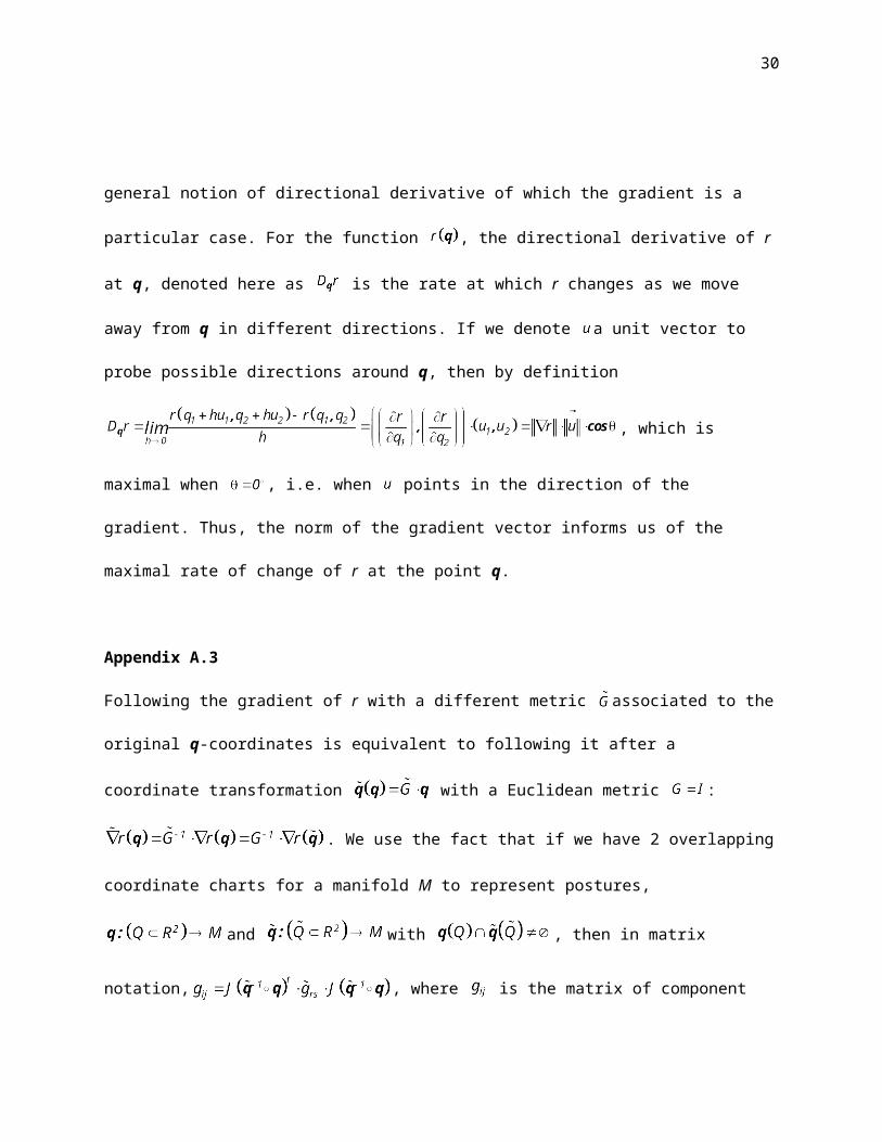
space. This comes from the general notion of directional derivative of which the gradient is a particular

case. For the function , the directional derivative of r at q, denoted here as is the rate at which r

changes as we move away from q in different directions. If we denote a unit vector to probe possible

18

directions around q, then by definition

, which is maximal when

, i.e. when points in the direction of the gradient. Thus, the norm of the gradient vector informs

us of the maximal rate of change of r at the point q.

Appendix A.3

Following the gradient of r with a different metric associated to the original q-coordinates is equivalent

to following it after a coordinate transformation with a Euclidean metric :

. We use the fact that if we have 2 overlapping coordinate charts for a

manifold M to represent postures, and with ,

then in matrix notation, , where is the matrix of component functions

of the metric associated to , is the matrix of component functions of the metric associated to , and

is the Jacobian matrix associated to the mapping , so that in

summation notation, (Gray 98). Because these coordinate charts overlap,

is invertible. Its inverse and . The

transformation rule (the chain rule) yields and multiplication by the inverse Jacobian

19

on both sides gives , i.e. the gradient of r with respect to the

-coordinates, for the Euclidean metric

Appendix A.4

The coefficients of the new metric due to a change of coordinates under the old metric can be obtained

and yield the same matrix as in (5): (Gray 1998)

where,

and

as in (5).

Appendix A.5

Given , we define the error:

20

set and minimize E with respect to B to solve for it and obtain .

21

Text Footnote

We impose the symmetric-positive-definite constraint to ensure a coordinate transformation that

preserves the properties of a space with a Euclidean inner-product.

22

Acknowledgments

Grant number Grant number 3 F31 NS10109-05S1 (to E. Torres) and grant number ICS9820 (systems

Developments to D. Zipser) supported this research. We want to thank Emo Todorov, Jude Mitchell and

Hans Christian Gromoll for all their very useful suggestions and comments.

23

Tables

Sh-abd Sh-flex Sh-pron Elb-flex Elb-pron Wr-abd Wr-flex

S1 0.0016 0.0039 0.0035 0.016 0.0044 0.0197 0.0189

S2 0.0015 0.0032 .00032 0.0097 0.0035 0.0231 0.0270

S3 0.0019 0.0021 0.0030 0.0139 0.0034 0.0218 0.0219

S4 0.0010 0.0021 0.0018 0.0101 .0.005 0.0283 0.0212

S5 0.0011 0.0014 0.0016 0.0083 0.0021 0.0112 0.0099

S6 0.0016 0.0016 0.0031 0.0137 0.0046 0.0201 0.0142

Table 1: Average mean absolute deviations from the difference between model and data (6 subjects).

24

Fitting Matrix Sh-abd Sh-flex Sh-pron Elb-flex Elb-pron Wr-abd Wr-flex

Least Square 0.0004 0.0007 0.0003 0.0012 0.0026 0.0105 0.0106

Symm Pos Def 0.0023 0.0040 0.0041 0.0040 0.0053 0.0242 0.0200

Table 2: Average mean absolute deviations from the difference between model and data (1 subject in the

2-different-initial-postures experiment).

25

Fitting Matrix Sh-abd Sh-flex Sh-pron Elb-flex Elb-pron Wr-abd Wr-flex

Least Square 0.0024 0.0016 0.002 0.0054 0.0035 0.0115 0.0206

Symm Pos Def 0.0029 0.0048 0.0033 0.0110 0.0053 0.0126 0.0267

Table 3: Average mean absolute deviations from the difference between model and data (1 subject in the

2-different-target-orientation experiment).

26

Figure Captions

Figure 1:

The arm is modeled as a system of 3 rigid-body segments. The Euler-Angle sequence XYZ is used to

model a 7 dof arm. The shoulder has a ball-and-socket joint with 3 dof, abduction-adduction ,

flexion-extension and pronation-supination . The elbow joint has 2 dof, flexion-extension

and pronation-supination . The wrist joint also has 2 dof, abduction-adduction and flexion-

extension . There is a fixed frame at the shoulder and 3 moving frames, one at each joint. The

position and orientation of each frame are described relative to the previous frame by

. The kinematics chain is used to describe position and

orientation of each joint relative to the fixed shoulder frame by:

where endpoint positions at shoulder, elbow, wrist and hand are given relative to the shoulder fixed frame

by: , , ,

Figure 2:

Matching the orientation of the hand to that of the target for a successful grasp: The matrix that represents

a rotation that will align the target with the hand is given by , where O represents the given

target orientation, and the hand’s orientation is represented by .

The rotation encoded in R can be represented by a single angle about the principal axis. This angle is

used in the cost function. When the hand matches the orientation of the object.

27

Figure 3:

Change of Metric: A Simple Example. When we change the metric (norm, inner product) of Q-space, we

affect the paths selected by the gradient. Panel (A) on the left shows the cost surface and the gradient-

generated solution for a given target under Euclidean metric, . The right panel shows the path

in X corresponding to this path in Q, and some of the posture sequence of the movement. Panel (B) shows

a change of metric in Q that under the old parameters gives straight-line paths in X (see

Appendix A.4 for the derivation of the new symmetric-positive-definite matrix ). Panel (B) shows the

new cost surface on the left and corresponding hand path in X on the right.

Figure 4:

A different -coordinate representation of postures associated to a Euclidean metric yields straight-line

paths in X. The matrix accomplishes the appropriate coordinate transformation to achieve this

constraint. In (A) and gives the original coordinates. In (B) and

. The new coordinates are

Figure 5:

An example of metric correction to implement “shortest-distance” paths on a sphere. Comparison of the

gradient-based solution path under Euclidean metric (--) and under a ‘natural’ metric (-) for the sphere

using the coordinates: , where and

are the azimuth and the elevation angles respectively, and .

28

Figure 6:

Constraining the elevation angle to move efficiently (in the minimum effort sense). (A) Compares the

paths in 3-space produced by the ‘plain gradient’ (left) vs. the corrected gradient (right). (B) Shows the

scalar function and the surface it spans for , .

The function essentially ‘speeds up’ movements towards rest and ‘slows down’ movements away from

rest, at the shoulder joint. In this parameterization, , and the elevation angle has index .

For any given posture , where is between 0 and , the second term in the exponential will be

negative. If the corresponding dq is negative, i.e. it ‘wants’ to move the arm away from rest (towards ),

the term within brackets in the exponential is positive and the negative exponential goes to 0, so the

gradient component dq2 is multiplied by a small positive constant . This slows down the rate of

change of that joint. If the current increment dq2 is positive, thus bringing the arm towards rest, the

expression within the brackets in the exponential is negative. Therefore, the exponential is a large positive

value in the denominator that makes the second term in the sum go to 0. The dq2 is multiplied by a large

positive constant , which increases the rate of change of that joint. The overall effect is a more

human-like motion of the arm.

Figure 7:

Experimental example of metric correction: Unconstraint arm movement paths were recorded from 6

subjects who performed orientation-matching motions to 6 targets located throughout the reachable

workspace and oriented differently. Circled paths are the subjects’ averaged across 6 repetitions.

Superimposed are the model’s paths obtained after the change of metric under the original coordinates, or

equivalently, after a coordinate transformation in Euclidean space. Table 1 shows the mean absolute

deviations per joint for each subject averaged across all 6 targets. They were obtained in the following

way: For each subject, per target, we compute the difference between the average data path (across 6

29

repetitions) and the corresponding model path, obtain the mean, subtract each value from it, take absolute

values, and then find the mean of the result.

Figure 8:

Effect of starting posture on position hand paths (A), posture paths (B), and orientation hand paths (C).

Two different starting postures are used to make orientation-matching motions to the same target position

and orientation. The model predicts a difference in postural paths and consequently on the hand position

and orientation paths. We have confirmed this prediction experimentally (details presented elsewhere). In

the figure, the data paths from one subject to one target (averaged over 6 repetitions) are plotted against

the model-generated paths. The broken-line paths correspond to the gradient-generated path assuming

Euclidean metric. The circled paths are from the hand position and orientation sensor data (the latter in

quaternion form). The superimposed dotted-line paths are those obtained after the change of metric using

. In figures A and C, we relaxed the symmetric-positive-definite

constraint in the computation of and computed the best fit in the least square sense. Figure B and

table 2 show there is a larger error in the corrected paths when we constraint the matrix to be symmetric-

positive-definite. Note that in this case, the matrix has to account for 2 very different postural paths in

configuration space. The larger error hints at the need to compute G as a function of posture.

Figure 9:

Effect of target orientation on position hand paths (A), posture paths (B), and orientation hand paths (C).

The model predicts that movements starting from the same initial posture towards a target located at the

same position, but oriented differently cause differences in the arm postural paths, and in the

corresponding hand position and orientation paths. Position hand paths produced by the gradient method

30

in a Euclidean space are shown as broken lines. We also show experimental data corresponding to one

subject’s sensor hand path (averaged across 6 repetitions) (circled lines) superimposed on the paths

generated by the model after the metric correction. The task was to match 2 different orientations, as if

grasping the cylinder from above (palm faces down) vs. doing so from below (palm faces up). Subjects

were holding a cylinder to match the target orientation with it and avoid the obstacle avoidance problem

that arises from the interactions between the fingers and the object to be grasped at the end of the

movement. Panel B shows the joint angle paths recovered from the position and orientation sensor data

superimposed on the model-generated paths. The symmetric-definite-positive matrix used to correct the

gradient is also shown here. Panel C compares the sensor orientation hand path (circled lines) and those

obtained from the model (dotted lines).

Figure 10:

The Gradient Descent approach permits on-line error correction because it receives continuous updated

feedback about the actual configuration of the arm. (A) Two different levels of random noise have been

applied to the gradient vector components at each time step, light and dark dotted paths. These paths are

perturbed, but the hand gets to the target. The smooth path is generated by the gradient without noise. (B)

The Gradient Descent approach permits to correct on-line perturbations of target position because it

receives continuous feedback from the current visual goal in the form of target position and orientation. In

the next time step it will compensate for the change in target position and output a signal that correctly re-

directs the hand to the new target.

31

Figure 11:

The gradient method can generate arbitrary trajectories. This figure shows a hand-written pattern,

represented by a stream of input targets, traced out by the hand. Several frames are selected to show some

of the postures in the sequence. Notice the smooth transition from posture to posture. This is achieved by

using the posture for each point in the pattern as the starting posture for moving to the next given target

position.

32

References:

Alexander, R. M. (1997). A minimum energy cost hypothesis for human arm trajectories. Bilogical

Cybernetics 76: 97-105.

Altman, S. L. Rotations, Quaternions and Double Groups. Oxford University Press, 1986, p.65-79.

Atkeson, C. G., and Hollerbach, J.M (1985). Kinematics Features of unrestrained vertical arm

movements. Journal of Neuroscience 5: 2318-2330.

Benati, M., Gaglio, S., Morasso, P.,Tagliasco, V., Zaccaria, R. (1980). Anthropomorphic Robotics (I).

Representing Mechanical Complexity. Biological Cybernetics 38: 125-40.

Bernstein, N. A. (1967). The Coordination and Regulation of Movements. London, Pergamon Press.

Bullock, D. and Grossberg, S. (1988). Neural dynamics of planned arm movements: Emergent invariants

and speed-accuracy properties during trajectory formation. Psychological Review, 95: 49–90

Castiello, U., Bennett, K., Chambers, H. (1998). Reach-to-Grasp: The response to a simultaneous

perturbation of object position and size. Experimental Brain Research 120: 31-40.

Desmurget, M., Grea, H., Prablanc, C. (1998). Final Posture of the Upper Limb Depends on the Initial

Position of the Hand During Prehension Movements. Experimental Brain Research 119(4): 511-516.

33

Desmurget, M., Prablanc, C. (1997). Postural Control of Three-Dimensional Prehension Movements.

Journal of Neurophysiology 77(1): 452-464.

Flash, T., Hogan, N (1985). The coordination of arm movements: an experimentally confirmed

mathematical model. The Journal of Neuroscience 5(7): 1688-1703.

Harris, C. M., Wolpert, Daniel M. (1998). Signal-dependent noise determines motor planning. Nature

394(20): 780-784.

Hinton, G. (1984). Parallel Computations for Controlling the Arm. Journal of Motor Behavior 16(2): 171-

194.

Hoff, B. and Arbib M.A. (1993). Models of trajectory formation and temporal interaction of reach and

grasp. Journal of Motor Behavior 25 (3):175-192.

Kalaska, J. F., Cohen, D.A.D., Hyde, M.L. and Prud'homme, M. (1990). Parietal Area 5 neuronal activity

encodes movement kinematics, not movement dynamics. Experimental Brain Research 80: 351-364.

Kowler, E. (1989). Cognitive Expectations, not habits, control anticipatory smooth oculomotor pursuit.

Vision Research 29(9): 1049-57.

Nishikawa K.C., M. S. T., and Flanders M. (1999). Do Arm Postures Vary with the Speed of Reaching?

Journal of Neurophysiology 81: 2582-2586.

34

Prablanc, C., Martin, O. (1992). Automatic Control During Hand Reaching at Undetected Two-

Dimensional Target Displacements. Journal of Neurophysiology 67: 455-469.

Shilov, G. E. (1968). Generalized Functions and Partial Differential Equations.(Theorem p.50-53). New

York, London, Paris, Gordon and Breach.

Soetching, J., Buneo, C., Flanders, M. (1995). Moving effortless in three dimensions: Does Donders'Law

apply to arm movement? The Journal of Neuroscience 15(9): 6271-6280.

Torres, E.B. (2001). Theoretical Framework for the Study of Sensori-motor Integration. Cognitive Science. La Jolla, University of California, San Diego: 115.

Uno, Y., Kawato, M., Suzuki, R. (1989). Formation and control of optimal trajectory in human multijoint

arm movement. Minimum torque-change model. Biological Cybernetics 61: 89-101.

35