Elliptic Cohomology - Prospects in Mathematics Durham, December 2006 Sarah Whitehouse
4 Elliptic curves
5 Elliptic cohomology
7 What is elliptic cohomology really?
Overview
What is elliptic cohomology?
• It’s a cohomology theory. For each topological space X , we have a graded ring Ell∗(X ), the elliptic cohomology of X .
• There are various different versions. In some sense there’s one version Ell∗C (−) for each elliptic curve C , hence the name. This provides a strong connection to number theory.
• It’s also related to theoretical physics - string theory and conformal field theory.
• The current definition is via homotopy theory.
• It’s a very active research area, especially the search for a more geometric definition.
A very brief history
• 1980’s: Witten: invariants of manifolds related to string theory, “physical” proof of a mysterious connection with elliptic curves
• 1980’s, 1990’s: Ochanine, Landweber, Stong, Ravenel: elliptic genus and first versions of elliptic cohomology
• 1980’s, 1990’s: Segal: “elliptic objects” - relation with conformal field theory
• Early 2000’s: Ando, Hopkins, Strickland: good homotopy theory definition of all elliptic theories
• Early 2000’s: Hopkins, Lurie, Miller: homotopy theory construction of the “universal elliptic cohomology”, tmf ∗(−)
• Now: ongoing search for a geometric or analytical or physical description
Invariants
In algebraic topology we assign invariants to topological spaces X .
topological spaces algebraic gadgets of some kind
Examples
X 7→ H∗(X ) or H∗(X ).
H∗(X ) is a graded abelian group and H∗(X ) is a graded ring.
• Complex K -theory
Cohomology theories
Topologists’ favourite invariants are cohomology theories. A cohomology theory E ∗(−) assigns to each topological space X a Z-graded abelian group E ∗(X ). This means that we have an abelian group E n(X ), for each integer n.
• This is done in such a way that E ∗(−) shares many of the basic properties of ordinary cohomology.
• In particular, standard techniques for calculation are available.
• Each example provides both a homology theory and a cohomology theory, “dual” to each other.
• Interesting examples have a multiplication: E ∗(X ) is a graded ring.
Genera
An elliptic cohomology theory will be a cohomology theory somehow associated to an elliptic curve. To explain how this association takes place, we will need to discuss genera and their associated log series.
A genus is a special sort of invariant. This is defined for manifolds.
An n-dimensional manifold is a compact space M which is locally homeomorphic to Rn, with some additional structure allowing differentiation. A manifold with boundary is like a manifold except that some points have neighbourhoods that look like Rn−1 × [0,∞) rather than Rn.
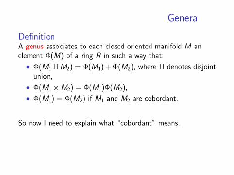
Genera
Definition A genus associates to each closed oriented manifold M an element Φ(M) of a ring R in such a way that:
• Φ(M1 qM2) = Φ(M1) + Φ(M2), where q denotes disjoint union,
• Φ(M1 ×M2) = Φ(M1)Φ(M2),
So now I need to explain what “cobordant” means.
Cobordism
Let M1, M2 be closed oriented manifolds of dimension n.
Definition M1 and M2 are cobordant if there is an oriented manifold W of dimension n + 1 such that ∂W = M1 q−M2.
This is an equivalence relation and we write MSOn for the set of equivalence classes. Then MSO∗ (that is the collection of MSOn for n ≥ 0) forms a graded ring, where the operations come from disjoint union and Cartesian product:
[M1] + [M2] = [M1 qM2],
[M1][M2] = [M1 ×M2].
2 ] = Z[1
2 ][x1, x2, x3, ...], a polynomial ring on
infinitely many variables, with xi in degree 4i .
The generators can be taken to be the classes of the even dimensional complex projective spaces [CP2i ].
We can also generalise the above construction, to define a homology theory.
Cobordism as a homology theory
Given a space X , we consider maps f : M → X , imposing the equivalence relation : f1 : M1 → X and f2 : M2 → X are equivalent if there is F : W → X such that the restriction to the boundary of W gives f1 q−f2 : M1 q−M2 → X .
Definition The set of equivalence classes is denoted MSO∗(X ).
Then X 7→ MSO∗(X ) is a homology theory. The first case we considered corresponds to taking X to be a point.
Logs
Now we can reformulate the definition of a genus as a ring map φ from MSO∗ to a graded ring R∗. We simplify matters by assuming 1
2 ∈ R∗ and consider
φ : MSO∗ ⊗ Z[1 2 ]→ R∗.
Then, by Thom’s theorem, a genus is completely determined by what it does on the generators xi = [CP2i ]. This is recorded in the associated log series:
logφ(x) = ∑ i≥0
2i + 1 x2i+1
in R ⊗Q[[x ]]. And, in fact, providing such a log series is equivalent to providing a genus.
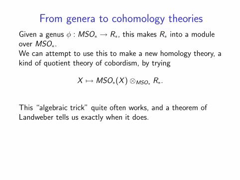
From genera to cohomology theories
Given a genus φ : MSO∗ → R∗, this makes R∗ into a module over MSO∗. We can attempt to use this to make a new homology theory, a kind of quotient theory of cobordism, by trying
X 7→ MSO∗(X )⊗MSO∗ R∗.
This “algebraic trick” quite often works, and a theorem of Landweber tells us exactly when it does.
The story so far I
nice cohomology ←→ nice genera theories i.e. ring maps
X 7→ E ∗(X ) MSO∗ → R∗
We need to explain how to produce a genus, and so a cohomology theory, from an elliptic curve.
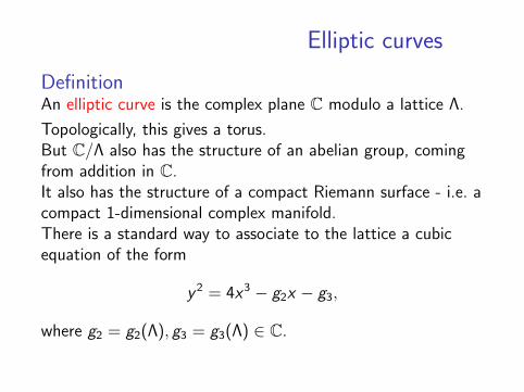
Elliptic curves
Definition An elliptic curve is the complex plane C modulo a lattice Λ.
Topologically, this gives a torus. But C/Λ also has the structure of an abelian group, coming from addition in C. It also has the structure of a compact Riemann surface - i.e. a compact 1-dimensional complex manifold. There is a standard way to associate to the lattice a cubic equation of the form
y 2 = 4x3 − g2x − g3,
where g2 = g2(Λ), g3 = g3(Λ) ∈ C.
Elliptic cohomology
Let C be an elliptic curve. Write its equation as
y 2 = 4(x − e1)(x − e2)(x − e3).
Let δ = −3 2 e1, ε = (e1 − e2)(e1 − e3).
Then, under a standard change of variables, its equation becomes the Jacobi quartic:
v 2 = 1− 2δu2 + εu4.
Definition For an elliptic curve C , the associated log series is given by the elliptic integral:
logφC (x) =
φC : MSO∗ → Z[1/2][δ, ε].
If the discriminant = ε2(δ2 − ε) is non-zero, then this satisfies the conditions necessary to produce a cohomology theory via Landweber’s theorem, giving Ell∗C (−).
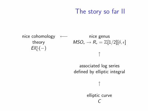
The story so far II
↑
↑
Modular forms
The value of elliptic cohomology on a point is closely related to modular forms. We can think of a lattice Λ in C as generated by 1 and z for some z in the upper half plane (up to isomorphism of elliptic curves). If we change z by z 7→ az+b
cz+d , where a, b, c and d are integers
and the determinant of the matrix
( a b c d
) is 1, we get an
isomorphic elliptic curve. The group of such matrices is SL(2, Z).
Modular forms
Definition A modular function of weight n is an analytic function f : H → C on the upper half H of the complex plane such that
f ((az + b)/(cz + d)) = (cz + d)nf (z)
for all matrices
) in SL(2, Z).
A modular function is a modular form if it is well-behaved as Im(z)→∞. There are only non-zero modular forms for weights which are natural numbers.
Modular forms
There is a graded ring of modular forms: if you add two modular forms of weight n you get another one of weight n, and if you multiply two modular forms of weights m and n, you get one of weight m + n.
There are lots of variants, corresponding to restricting to subgroups of finite index in SL(2, Z).
One variant turns out to give the graded ring Z[1/2][δ, ε], with δ in degree 4 and ε in degree 8. It is not a coincidence that this is the same ring that showed up earlier: it’s not hard to see that the elliptic genus we defined earlier takes values in this ring of modular forms.
A universal elliptic cohomology?
To an elliptic curve we have associated a cohomology theory.
elliptic curve C 7→ Ell∗C (−)
Then Ell∗C (−) is (an) elliptic cohomology. So there are many elliptic cohomologies, not just one. We would like to say: take the “universal elliptic curve” and then the associated cohomology theory is the (universal) elliptic cohomology. Unfortunately, the “universal elliptic curve” doesn’t exist. Nonetheless, it is possible to define a kind of universal elliptic cohomology, called tmf ∗(−), short for “topological modular forms”. It’s universal in the sense that it comes with a good map to any elliptic cohomology theory.
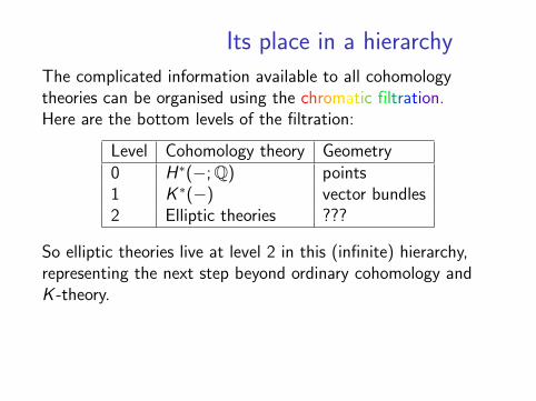
Its place in a hierarchy
The complicated information available to all cohomology theories can be organised using the chromatic filtration. Here are the bottom levels of the filtration:
Level Cohomology theory Geometry 0 H∗(−; Q) points 1 K ∗(−) vector bundles 2 Elliptic theories ???
So elliptic theories live at level 2 in this (infinite) hierarchy, representing the next step beyond ordinary cohomology and K -theory.
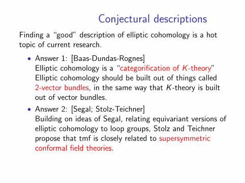
Conjectural descriptions
Finding a “good” description of elliptic cohomology is a hot topic of current research.
• Answer 1: [Baas-Dundas-Rognes] Elliptic cohomology is a “categorification of K -theory” Elliptic cohomology should be built out of things called 2-vector bundles, in the same way that K -theory is built out of vector bundles.
• Answer 2: [Segal; Stolz-Teichner] Building on ideas of Segal, relating equivariant versions of elliptic cohomology to loop groups, Stolz and Teichner propose that tmf is closely related to supersymmetric conformal field theories.
Advertising
We expect to have at least 5 funded Ph.D. places in Pure Mathematics in Sheffield next academic year.
We have strong research groups in algebraic topology, commutative algebra, differential geometry, number theory and ring theory.
Please look at our webpages at http://www.shef.ac.uk/puremaths/prospectivepg
Overview
Invariants
Elliptic curves
Elliptic cohomology