embedding naive bayes classification in a functional and object
TRANSCRIPT

IT 10 039
Examensarbete 30 hpAugusti 2010
Embedding Naive Bayes classification in a Functional and Object Oriented DBMS
Thibault Sellam
Institutionen för informationsteknologiDepartment of Information Technology


Teknisk- naturvetenskaplig fakultet UTH-enheten Besöksadress: Ångströmlaboratoriet Lägerhyddsvägen 1 Hus 4, Plan 0 Postadress: Box 536 751 21 Uppsala Telefon: 018 – 471 30 03 Telefax: 018 – 471 30 00 Hemsida: http://www.teknat.uu.se/student
Abstract
Embedding Naive Bayes classification in a Functionaland Object Oriented DBMS
Thibault Sellam
This thesis introduces two implementations of Naïve Bayes classification for thefunctional and object oriented Database Management System Amos II. The first one isbased on objects stored in memory. The second one deals with streamed JSONfeeds. Both systems are written in the native query language of Amos, AmosQL. Itallows them to be completely generic, modular and lightweight. All data structuresinvolved in classification including the distribution estimation algorithms can bequeried and manipulated. Several optimizations are presented. They allow efficientand accurate model computing. However, scoring remains to be accelerated. Thesystem is demonstrated in an experimental context: classifying text feeds issued by aWeb social network. Two tasks are considered: recognizing two basic emotions andkeyword-filtering.
Tryckt av: Reprocentralen ITCIT 10 039Examinator: Anders JanssonÄmnesgranskare: Tore RischHandledare: Tore Risch


TABLE OF CONTENTS
1 Introduction ....................................................................................................................................................... 1
2 Scientific background and related work ............................................................................................................ 2
2.1 The relationship between Databases and Data Mining ............................................................................. 2
2.2 Naïve Bayes classification ........................................................................................................................ 3
2.3 Naïve Bayes in SQL .................................................................................................................................. 7
2.4 Amos II: an extensible functional and objected-oriented DBMS ............................................................. 7
2.5 Learning from data streams..................................................................................................................... 10
3 Learning from and Classifying stored objects ..................................................................................................11
3.1 Principles and interface of the Naïve Bayes Classification Framework (NBCF) ....................................11
3.2 Data structures and algorithms of the NBCF .......................................................................................... 15
3.3 Performance evaluation........................................................................................................................... 18
4 Learning from and classifying streamed JSON Strings ................................................................................... 21
4.1 Principles and interface of the Incremental Naïve Bayes Classification Framework (INBCF) .............. 21
4.2 Implementation details and time complexity .......................................................................................... 23
4.3 Performance evaluation........................................................................................................................... 27
5 Application: Classifying a stream of messages delivered by a social network ................................................ 29
5.1 Preliminary notions ................................................................................................................................. 29
5.2 Tuning the INBCF .................................................................................................................................. 31
5.3 First application: a “naïve Naïve Bayes” approach to opinion mining ................................................... 32
5.4 Second application: a NB-enhanced keyword filter ................................................................................ 36
6 Conclusion and future work ............................................................................................................................. 37
7 Bibliography .................................................................................................................................................... 38

1
1 INTRODUCTION Data Mining consists in extracting knowledge automatically from large amounts of data. This knowledge can be relationships between variables (association rules), or groups of items that would be similar (clusters). It can also
be classifiers, e.g. functions mapping data items to classes given their features. This thesis deals with the latter. A feature is a stored attribute of an item. This could the size of a person or the content of an email. The class is the value of a given attribute that is to be predicted. For instance it could be someone’s gender or the quality “spam”
or “non spam” of an email. The possible classes are finite and predetermined.
This thesis is based on the supervised learning approach. Two successive steps involving each a data set are discussed: the training phase and the classification phase. The first phase involves building a classifier with items which classes are known. These elements are the training set. Then, the obtained function is applied on a second
set of items to predict their class. Consider for instance spam detection. A classifier is first trained with a set of emails manually labeled “spam” or “legitimate”. Then, it can predict the class of emails it has never encountered before.
The problem studied in this thesis is the following: how should a classification algorithm be implemented in a Database Management System (DBMS)? Indeed, a traditional way to operate classification is to store the datasets
in a DBMS and run the algorithms with an external application. The studied data sets are entirely copied to the application memory space. This allows fast treatments, as the calculations are based on fast main memory
languages such as C or Java. However, performing the classification directly in the database also presents advantages. Firstly, DBMSs scale well with large datasets by nature. Secondly, in-base classification tools avoid developing redundant functions. Indeed, many operations required by data mining tasks such as counting or
sorting are already offered by the database query language. Finally, such functionalities would increase the database user productivity: a developer should not create his own ad-hoc solution each time he needs classification tools. This thesis proposes two classification algorithms for the functional and object oriented
DBMS Amos II[1].
Many methods have been introduced to perform classification. This work is based on Naïve Bayes, which shows high accuracy despite its simplicity [2]. Naïve Bayes is a generative technique. This means that it generates probability distributions for each class to be predicted. Consider for instance a training set based on some
individuals whose sizes and genders are known. If the classes to be learnt are the genders, two distributions will be built: one represents the size given the gender “male”, the other the size given “female”. Classifying an individual whose gender is unknown and whose size is known implies comparing the probabilities that it is a male
or a female given his size. This is performed thanks to Bayes’ theorem. Naïve Bayes is more a generic technique than a particular algorithm. Indeed, many variant have been introduced. This thesis uses and extends the one
described in [3]. Amos II is a main memory Database Management System (DBMS) which allows multiple, heterogeneous and
distributed data sources to be queried transparently [1]. The first objective of this work is to extend this system with classification functionalities in a fully integrated and generic fashion: the Naïve Bayes Classification Framework (NBCF) is introduced. The proposed algorithms are based on the database items and their properties
as they are stored in the system. The classifier, the classification results, but also the modeling techniques themselves are objects that can be queried, manipulated and re-used. In particular, this modularity allows dealing easily with mixed attribute types. For instance, given a population, one feature could be modeled by a Gaussian
distribution object while another is binned and counted in frequency histograms.
AmosQL is the functional query language associated with the data model of Amos II. Its expressivity allows the Naïve Bayes classification framework (NBCF) to be simple and particularly lightweight. Nevertheless, it has more overhead than a “traditional” main memory imperative language. Therefore, evaluating how it performs in a
scaled data mining context and leveraging it for learning is the second objective of this study. Recently, Amos II has acquired data streams handling functionalities. With data streaming, the items do not need
to be stored in the database. Instead, they are “passing through” the system once without occupying any persistent memory. The NBCF was made incremental in order to support such setup: this is the Incremental Naïve Bayes
Classification Framework (INBCF). The NBCF generates a classifier from a finite set of items. Its incremental version generates an “empty” classifier and improves (updates) it each time one or several streamed items are met.

2
This supposes two changes. Firstly, all maintained statistics have to be computed in one pass as the training items
are not stored. Secondly, since the mining has to be operated on temporarily allocated ad-hoc objects, the INBCF will learn from and classify JSON strings (JavaScript Object Notation) [4]. Indeed, this format is fully supported
by Amos II, and it appears to be one of the most used and simplest representation standards. As a proof of concept of the ICNBF, the final part of this work presents two applications based on the popular
social network Twitter [5]. Twitter delivers streams of JSON objects describing all messages that are posted by users from in quasi-real time. An Amos II wrapper for JSON streams was used [6]. Two experiments were made:
- The first classification task is to recognize enthusiasm or discontent in messages. Two sets of words
identifying negative or positive examples allow automatic labeling of the learning examples. The training phase builds the distribution of words in these messages. The classification matches messages against the
trained distributions to identify positive, negative, or neutral messages. - The second example filters twitter streams given a set of keywords. The training phase computes the
distribution of words in messages that are relevant w.r.t. the set. The classification matches messages
against these learned distributions.
2 SCIENTIFIC BACKGROUND AND RELATED WORK
2.1 The relationship between Databases and Data Mining
Data Mining, or Knowledge Discovery, is a process of nontrivial extraction of implicit, previously unknown and potentially useful information from a database [7]. According to [8], the past and current research in this field can be categorized in 1) investigating new methods to discover knowledge and 2) integrating and scaling these
methods. This work focuses on the last aspect.
In [9], a “first generation” of data mining tools is identified. These tools rely on a more or less loose connection
between the DBMS and mining system: a front end developed with any language embeds SQL select statements and copies their results in main memory. Then, one stake for database research is to optimize the data retrieving
operations and allow fast in-base treatments, in order to tighten the connection between the front end and the DBMS.
Indeed, making efficient use of a query language is nontrivial, and could bring up nice performance and usability enhancements. For instance, multiples passes through data using different orders may involve SQL sorting and
grouping operations. This can be done with database tuning techniques, such as smart indexing, parallel query execution or main memory evaluation. [8] also notices that SQL can be leveraged and computation staged. Therefore data mining applications should be “SQL aware”.
Tightening this connection is also one of the purposes of object oriented databases, Turing complete programming
languages embedded in most systems, such as PL/SQL (Oracle), and user defined functions developed in another language. [10] presents a tightly-coupled data mining methodology in which complete parts of the knowledge discovery operations are pushed into the database to avoid context switching costs and intermediate results storage
in the application space. The following section deals classification operations written directly in SQL. Finally, in the software industry, Microsoft SQL Server 2000 introduced in-base data mining classification and rule discovery tools.
Oppositely, [11] justifies complete loose coupling. Indeed, the cost of memory transfers from the DBMS to the application may cancel all the benefits of executing some operations such as counting or sorting directly in the
database. SQL also suffers from a lack of expressivity: some operations that could be realized in one pass with a procedural language may require more with SQL. Therefore, the optimal way is to load the data in main memory
with a select statement “once and for all”, and perform all operations in this space. [8] notes one major challenge for the field of data mining research: the ad-hoc nature of the tasks to be handled.
Therefore, scaling efforts should not be applied on specific algorithms such as APriori or decision trees[11], but on their basic operations. Improvements for SQL are proposed. One a first level, new core primitives could be
developed for operations such as sampling or batch aggregation (multiple aggregations over the same data). The
generalization of the CUBE operator [12] is a step in this direction. On a higher level, data mining primitives could be embedded, such as support for association rules [13].

3
A long term vision of these principles is exposed in [9]: “second generation” tools, Knowledge Discovery Data Management Systems (KDDMS) are introduced. SQL could be generalized to create, store and manipulate “KDD
objects”: rules, classifiers, probabilistic formulas, clusters, etc… The associated queries (“KDD queries”) should be optimized and support a closure principle: the result of a query can itself be queried. In this perspective, Data Mining Query Languages have been introduced these past years. Among many others, MSQL [14] and DMQL
[15] are representative of this effort.
2.2 Naïve Bayes classification
2.2.1 Supervised learning
Consider for instance the following data set describing the features of 5 individuals:
Item Hair Size (cm) Sex
𝑋1 Short 176 Male
𝑋2 Short 189 Male
𝑋3 Long 165 Female
𝑋4 Short 175 Female
𝑌 Short 174 ?
Fig. 1: an example of supervised learning data
The classification task is to recognize the sex of a person. There are two classes 𝐶 = *𝐹𝑒𝑚𝑎𝑙𝑒,𝑀𝑎𝑙𝑒+. The data
set can be decomposed in two subsets:
- The items which classes are known *(𝑋1,𝑀𝑎𝑙𝑒), (𝑋2,𝑀𝑎𝑙𝑒), (𝑋3, 𝐹𝑒𝑚𝑎𝑙𝑒), (𝑋4, 𝐹𝑒𝑚𝑎𝑙𝑒)+. They
constitute the training (or learning) set.
- An item 𝑌 = (𝑆𝑜𝑟𝑡, 174) which classes is unknown. It is a test item.
The goal of supervised learning is to infer a classifier from the training set and apply it on the test item to predict its class.
The training set will be referred to as *(𝑋𝑖, 𝑐𝑖)+𝑖∈,1,𝑝- with 𝑋𝑖 = (𝑥𝑖1, 𝑥𝑖
2, 𝑥𝑖3, … , 𝑥𝑖
𝑛) and 𝑐𝑖 ∈ 𝐶. Each component
𝑥𝑖𝑗 will be referred to as attribute, or feature, taking its value in a space defined by the classification problem
(either continuous or discrete). The test item will be represented by 𝑌 = (𝑦1, 𝑦2, 𝑦3, … , 𝑦𝑛). The classifier returns
its class 𝑐𝑌
Supervised learning is a wide field of computer science and applied mathematics [16]. Among many others, neural networks, support vector machines, decision trees and nearest neighbor algorithms have been well established techniques. This thesis is based on Naïve Bayes (NB). The following reasons justify this choice:
- NB-based techniques are usually very simple. They involve basic numeric operations, which makes them well suited to a DBMS implementation
- NB can deal with any kind of data (continuous or discrete inputs) - NB is known to be robust to noise (in the data or in the distribution estimation) and high dimensionality
data [2]
2.2.2 Presentation of Naïve Bayes
𝑋𝑘 is the random variable representing the 𝑘𝑡ℎ feature of an item. 𝐶 is the random variable describing its class.
For readability’s sake, 𝑃(𝑋𝑘 = 𝑎𝑘) will be abbreviated as 𝑃(𝑎𝑘), ak being a constant expression. Similarly,
𝑃(𝐶 = 𝑐) will be abbreviated as 𝑃(𝑐)
Procedure
With Naïve Bayes, classifying an item (𝑦1, 𝑦2, 𝑦3,… , 𝑦𝑛) consists in computing 𝑃(𝑐𝑖| 𝑦1 ∧ 𝑦2 ∧ … ∧ 𝑦𝑛) for
each class 𝑐𝑖. The class giving the highest score will be selected. However, this probability can generally not be
calculated as such. Naïve Bayes classification relies on the assumption that each attribute is conditionally independent to every other
attributes, i.e.:
4
(1) 𝑃(𝑎𝑘 | 𝑐 ∧ 𝑎𝑙) = 𝑃(𝑎𝑘 | 𝑐 )
with 𝑘 ≠ 𝑙 and 𝑎𝑘, 𝑎𝑙 , c constant expressions.
Under this assumption, 𝑃(𝑐𝑖| 𝑦1 ∧ 𝑦2 ∧ … ∧ 𝑦𝑛) ≈ 𝑃(𝑐𝑖)𝑃(𝑦
1|𝑐𝑖)𝑃(𝑦2|𝑐𝑖)…𝑃(𝑦
𝑛|𝑐𝑖) for each class 𝑐𝑖. This simplification is fundamental.
Therefore, learning with Naïve Bayes consists in:
- estimating the prior distributions of the classes, e.g. the probability of occurrence of each class ��(𝐶 = 𝑐)
- approximating the distributions of the features given each class ��(𝑋𝑘 = 𝑎𝑘|𝑐𝑖) (in the example, the
distribution of sizes for males is one of these). The choice of the distribution approximation method depends on the task. For instance, a Normal distribution could be fitted over numerical data. Counting the
occurrences of the values of 𝑋𝑘in a frequency histogram is often a good solution for categorical values.
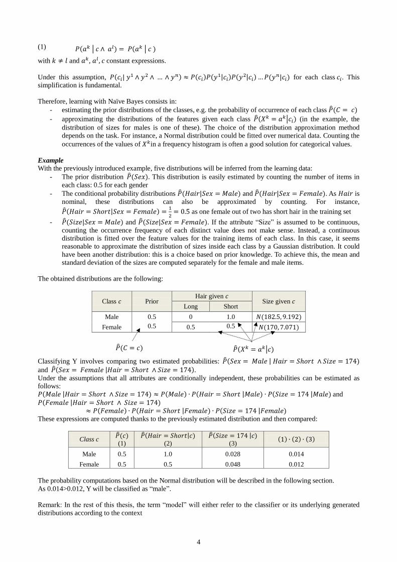
Example With the previously introduced example, five distributions will be inferred from the learning data:
- The prior distribution ��(𝑆𝑒𝑥). This distribution is easily estimated by counting the number of items in
each class: 0.5 for each gender - The conditional probability distributions ��(𝐻𝑎𝑖𝑟|𝑆𝑒𝑥 = 𝑀𝑎𝑙𝑒) and ��(𝐻𝑎𝑖𝑟|𝑆𝑒𝑥 = 𝐹𝑒𝑚𝑎𝑙𝑒). As 𝐻𝑎𝑖𝑟 is
nominal, these distributions can also be approximated by counting. For instance,
��(𝐻𝑎𝑖𝑟 = 𝑆𝑜𝑟𝑡|𝑆𝑒𝑥 = 𝐹𝑒𝑚𝑎𝑙𝑒) =1
2= 0.5 as one female out of two has short hair in the training set
- ��(𝑆𝑖𝑧𝑒|𝑆𝑒𝑥 = 𝑀𝑎𝑙𝑒) and ��(𝑆𝑖𝑧𝑒|𝑆𝑒𝑥 = 𝐹𝑒𝑚𝑎𝑙𝑒). If the attribute “Size” is assumed to be continuous,
counting the occurrence frequency of each distinct value does not make sense. Instead, a continuous distribution is fitted over the feature values for the training items of each class. In this case, it seems reasonable to approximate the distribution of sizes inside each class by a Gaussian distribution. It could
have been another distribution: this is a choice based on prior knowledge. To achieve this, the mean and standard deviation of the sizes are computed separately for the female and male items.
The obtained distributions are the following:
Class 𝑐 Prior Hair given 𝑐
Size given 𝑐 Long Short
Male 0.5 0 1.0 (1 2.5, .1 2)
Female 0.5 0.5 0.5 (170, 7.071)
Classifying Y involves comparing two estimated probabilities: ��(𝑆𝑒𝑥 = 𝑀𝑎𝑙𝑒 | 𝐻𝑎𝑖𝑟 = 𝑆𝑜𝑟𝑡 ∧ 𝑆𝑖𝑧𝑒 = 174) and ��(𝑆𝑒𝑥 = 𝐹𝑒𝑚𝑎𝑙𝑒 |𝐻𝑎𝑖𝑟 = 𝑆𝑜𝑟𝑡 ∧ 𝑆𝑖𝑧𝑒 = 174). Under the assumptions that all attributes are conditionally independent, these probabilities can be estimated as follows:
𝑃(𝑀𝑎𝑙𝑒 |𝐻𝑎𝑖𝑟 = 𝑆𝑜𝑟𝑡 ∧ 𝑆𝑖𝑧𝑒 = 174) ≈ 𝑃(𝑀𝑎𝑙𝑒) ∙ 𝑃(𝐻𝑎𝑖𝑟 = 𝑆𝑜𝑟𝑡 |𝑀𝑎𝑙𝑒) ∙ 𝑃(𝑆𝑖𝑧𝑒 = 174 |𝑀𝑎𝑙𝑒) and 𝑃(𝐹𝑒𝑚𝑎𝑙𝑒 |𝐻𝑎𝑖𝑟 = 𝑆𝑜𝑟𝑡 ∧ 𝑆𝑖𝑧𝑒 = 174)
≈ 𝑃(𝐹𝑒𝑚𝑎𝑙𝑒) ∙ 𝑃(𝐻𝑎𝑖𝑟 = 𝑆𝑜𝑟𝑡 |𝐹𝑒𝑚𝑎𝑙𝑒) ∙ 𝑃(𝑆𝑖𝑧𝑒 = 174 |𝐹𝑒𝑚𝑎𝑙𝑒) These expressions are computed thanks to the previously estimated distribution and then compared:
Class c ��(𝑐) (1)
��(𝐻𝑎𝑖𝑟 = 𝑆𝑜𝑟𝑡|𝑐) (2)
��(𝑆𝑖𝑧𝑒 = 174 |𝑐) (3)
(1) ∙ (2) ∙ (3)
Male 0.5 1.0 0.028 0.014
Female 0.5 0.5 0.048 0.012
The probability computations based on the Normal distribution will be described in the following section.
As 0.014>0.012, Y will be classified as “male”. Remark: In the rest of this thesis, the term “model” will either refer to the classifier or its underlying generated
distributions according to the context
��(𝑋𝑘 = 𝑎𝑘|𝑐) ��(𝐶 = 𝑐)

5
2.2.3 Justification and decision rules
Bayes’ theorem states that for a given tuple Y:
(2) 𝑃(𝑐 | 𝑎1 ∧ 𝑎2 ∧ … ∧ 𝑎𝑛) =𝑃(𝑐𝑌 = 𝑐) ∙ 𝑃(𝑎1 ∧ 𝑎2 ∧ … ∧ 𝑎𝑛 | 𝑐)
∑ 𝑃(𝑐𝑌 = 𝑐 ) ∙ 𝑃 ∈ (𝑎1 ∧ 𝑎2 ∧ … ∧ 𝑎𝑛 |𝑐 )
Then, using (1) and (2):
(3) 𝑃(𝑐 | 𝑎1 ∧ 𝑎2 ∧ 𝑎3 ∧ … ∧ 𝑎𝑛 ) = 𝑃(𝑐𝑌 = 𝑐) ∙ ∏ 𝑃 (𝑎𝑘 |𝑐 )𝑛
𝑘=1
∑ 𝑃(𝑐𝑌 = 𝑐 ) ∙ ∏ 𝑃(𝑎𝑘 |𝑐 )𝑛𝑘=1 ∈
The Maximum A Posteriori (MAP) rule can be applied to determine which class is most likely to cover Y:
(4) 𝑐𝑌 ← argmax ∈
𝑃(𝑐) ∙∏𝑃 (𝑎𝑘 |𝑐 )
𝑛
𝑘=1
The denominator of (3) has been omitted as it is the same for all classes.
Alternatively, if 𝐶 = *𝑐 , 𝑐1+, the class to which Y belongs can be deduced from :
(5) ln 𝑃(𝑐 | 𝑎
1 ∧ 𝑎2 ∧ … ∧ 𝑎𝑛)
𝑃(𝑐1 | 𝑎1 ∧ 𝑎2 ∧ … ∧ 𝑎𝑛)
= ln𝑃(𝑐 )
𝑃(𝑐1)+∑ln
𝑃( 𝑎𝑘 | 𝑐𝑌 = 𝑐 )
𝑃( 𝑎𝑘 | 𝑐𝑌 = 𝑐1 )
𝑛
𝑘=1
2.2.4 Approximating the distributions
Prior distributions
The prior probability over 𝑐𝑌, e.g. 𝑃(𝑐𝑌 = 𝑐), is approximated by counting all training items referring to class c,
divided by the total number of training items :
(6) ��(𝑐) = | *(𝑋𝑖, 𝑐𝑖)/ 𝑖 ∈ ,1, 𝑝-, 𝑐𝑖 = 𝑐+ |
𝑝
Attributes distributions - Discrete inputs
The probabilities ��(𝑎𝑘|𝑐𝑌 = 𝑐) can be obtained by dividing the number of training items of class c for which
𝑥𝑖𝑘 = 𝑎𝑘 by the number of training items in class c (frequency histogram):
(7) ��(𝑎𝑘| 𝑐) = | *(𝑋𝑖, 𝑐𝑖)/ 𝑖 ∈ ,1, 𝑝-, 𝑐𝑖 = 𝑐, 𝑥𝑖
𝑘 = 𝑎𝑘+ |
| *(𝑋𝑖, 𝑐𝑖)/ 𝑖 ∈ ,1, 𝑝-, 𝑐𝑖 = 𝑐+ |
If a test item contains an attribute 𝑦𝑘 set to 𝑎𝑘, and the classifier has never encountered 𝑎𝑘 before in a training
example marked 𝑐𝑖, then: ��(𝑎𝑘|𝑐𝑖) = 0. In this case, the whole estimation ��(𝑐) ∙ ∏ �� (𝑎𝑘 |𝑐 )𝑛𝑘=1 will be set to 0,
regardless of the likelihood induced by the other attributes. This effect may be too “harsh” for some classification
tasks (for instance, text classification): this is often called the “zero counts problem”. Many methods have been presented to “smoothen” the estimation, this thesis uses the virtual examples introduced in [16] :
(8) 𝑃′(𝑎𝑘| 𝑐) = | *(𝑋𝑖, 𝑐𝑖)/ 𝑖 ∈ ,1, 𝑝-, 𝑐𝑖 = 𝑐, 𝑥𝑖
𝑘 = 𝑎𝑘+ | + 𝑙
| *(𝑋𝑖, 𝑐𝑖)/ 𝑖 ∈ ,1, 𝑝-, 𝑐𝑖 = 𝑐+ | + 𝑙𝐽
𝐽 is the number of distinct values observed among 𝑥1𝑘, 𝑥2
𝑘, … , 𝑥𝑛𝑘. 𝑙 is a user-defined parameter. Typically, 𝑙 is set
to 1: in this case, (8) describes a Laplace smoothing.
Many other distribution estimations methods exist for discrete values. This thesis will also use Poisson and Zipf’s distributions fitting over the observed data.
Attributes distributions - Continuous inputs One approach to dealing with continuous values is to use value binning to treat them as discrete inputs. [3] (on
which this thesis is based) makes use of two methods. The first one involves k uniform bins between the extreme

6
values of an attribute. The second one is based on intervals around the mean, defined by multiples of the standard
deviation.
Alternatively, a continuous model can be generated to fit the observed values of an attribute. Often, continuous
features 𝑦𝑘 are e assumed to be distributed normally within the same class c, with a mean 𝜇 �� and standard
deviation 𝜎 �� inferred from the training examples:
(9) 𝜇 �� =
∑ 𝑥𝑖𝑘
𝑖∈,1,𝑝-, 𝑖=
| *(𝑋𝑖, 𝑐𝑖)/ 𝑖 ∈ ,1, 𝑝-, 𝑐𝑖 = 𝑐+ | , 𝜎
�� = ∑ (𝑥𝑖
𝑘 − 𝜇 𝑘)2 𝑖∈,1,𝑝-, 𝑖=
| *(𝑋𝑖, 𝑐𝑖)/ 𝑖 ∈ ,1, 𝑝-, 𝑐𝑖 = 𝑐+ | − 1
Then, as justified in [17], the following equation can be exploited:
(10) ��(𝑎𝑘|𝑐𝑌 = 𝑐) ≈ 𝑔 .𝑎𝑘, 𝜇 ��, 𝜎
��/ with the density function 𝑔 .𝑎𝑘, 𝜇 ��, 𝜎
��/ = 1
√2𝜋 𝜎 ��
𝑒
. /
2
The probability that a normally distributed variable 𝑦 equals exactly a value 𝑎 is null. However, using the
definition of derivative: lim∆→ 𝑃(𝑎 ≤ 𝑦 ≤ 𝑎 + ∆) ∆⁄ = 𝑔(𝑎, 𝜇, 𝜎), with 𝜇 and 𝜎 mean and standard deviation
of the considered distribution. Then, for ∆ close to 0, 𝑃(𝑦 = 𝑎) ≈ 𝑔(𝑎, 𝜇, 𝜎) ∙ ∆. In Naïve Bayes, as ∆ is
class-independent, it can be neglected without degrading the classification accuracy.
2.2.1 Measuring the accuracy of a classifier
In this thesis, three measurements are used (depending on the task) when confronting the predictions of classifiers
to those of an “expert” on a testing set.
Error rate
The error rate is obtained as follows:
𝑢𝑚𝑏𝑒𝑟 𝑜𝑓 𝑚𝑖𝑠𝑐𝑙𝑎𝑠𝑠𝑖𝑓𝑖𝑐𝑎𝑡𝑖𝑜𝑛𝑠
𝑆𝑖𝑧𝑒 𝑜𝑓 𝑡𝑒 𝑡𝑒𝑠𝑡𝑖𝑛𝑔 𝑠𝑒𝑡
The description of the classifier’s behavior by this measurement is quite weak. Nevertheless, when two classifiers are known to have a similar behavior (in this thesis, two implementation of the same algorithm), comparing error rates can provide information about their relative reliability.
Kappa statistic
The Kappa statistic measures the agreement between several “experts” on categorical data classification. This
indicator is based on the difference between the “observed” agreement 𝑔𝑟 and the agreement that labeling
the examples randomly would be expected to reveal, 𝑔𝑟 . It is calculated as follows:
𝑔𝑟 − 𝑔𝑟 1 − 𝑔𝑟
𝑔𝑟 is the proportion of test items on which the experts agree. Consider a binary classification context (two
classes, + and -) with 𝑝 test examples, if the experts classify respectively 𝑝1 and 𝑝2 examples as positive and 𝑛1
and 𝑛2 as negative, then 𝑔𝑟 = (𝑝1/𝑝 𝑝2/𝑝) + (𝑛1/𝑝 𝑛2/𝑝). This calculation can be directly generalized to more classes.
An interpretation “grid” is proposed in [18]:
- < 0: Less than chance agreement - 0.01–0.20: Slight agreement - 0.21– 0.40: Fair agreement
- 0.41–0.60: Moderate agreement - 0.61–0.80: Substantial agreement - 0.81–0.99 : Almost perfect agreement
These assessments are to be adapted to the context.

7
This indicator will be used to evaluate the accuracy of the Twitter “emotions” classifier presented in the last part.
Precision and recall
In binary classification (two classes, + and -), the following terminology may be used to describe the classifier’s predictions:
- Items from class + classified + are true positives - the quantity of true positives is TP
- Items from class - classified + are false positives - FP - Items from class - classified - are true negatives - TN - Items from class - classified + are false negatives - FN
The following indicators may be used:
𝑃𝑟𝑒𝑐𝑖𝑠𝑖𝑜𝑛 =𝑇𝑃
𝑇𝑃 + 𝐹𝑃 𝑅𝑒𝑐𝑎𝑙𝑙 =
𝑇𝑃
𝑇𝑃 + 𝐹
Intuitively, the precision represents the “purity” of the positive class. The recall describes the proportion of “real” positives that were classified as such.
The precision and the recall are useful to describe the accuracy of filters or search engines. In this scenario, the items of class – constitute “noise” that is to be detected and skipped. These indicators will be used when
evaluating a Twitter keyword-based filter.
2.3 Naïve Bayes in SQL
This work is a generalization of the approach presented in [3]. In this thesis, two full SQL Naïve Bayes implementations are introduced. The first one considers Naïve Bayes in its most common variant (cf. next section). It is implemented in a straightforward way. The second one is an extended version, proven to be often
more accurate: K-means are used to decompose classes into clusters. All implementation and optimization details for this second algorithm are given. For instance, indexes are fully made use of, and the table storing cluster
statistics is denormalized. In terms of performance, the authors show that for both algorithms, 1) for test item scoring, optimized SQL runs faster than calling user defined functions written in C 2) although C++ is four times faster for the same algorithm, exporting data via ODBC is a crippling bottleneck. The rest of this thesis applies to
the first algorithm. A similar work is introduced in [19]. Another implementation of Naïve Bayes in SQL is exposed. A main
difference is that it is based on a large pivoted table with schema (item_id, attribute_name,
attribute_value), shown inefficient in [3]. It can only deal with discrete attributes and does not support the K-
means enhancement.
The first part of the work presented here is quite close to these articles. The differences are the following: - The introduced framework is completely based on a functional object-oriented model instead of a
relational model. Although a model expressed in one paradigm can be translated into another, the
assumptions and optimizations techniques are quite different. Complex objects are directly manipulated for classification instead of tuples. Furthermore, Amos II runs in main memory, which induces different priorities.
- One focus of [3] and [19] is to present portable code, which could be embedded in any SQL dialect: only
basic primitives are used (no mean or variance). This work makes full use of Amos II data mining
operators as the classifier is designed for this system only. - These articles do not seem to give any information about how to deal with the ad hoc nature of the data.
As a matter of fact, a new SQL code for the complete framework is to be generated for each data mining
task, for a DBMS that would be dedicated to classification. Oppositely, integrating Naïve Bayes in the Amos II data model in a completely application-independent way is the main objective of this work.
2.4 Amos II: an extensible functional and objected-oriented DBMS
2.4.1 Overview
The following describes some of the features of Amos II [1][20].

8
General properties
- Amos II can manage locally stored data, external data sources as well as data streams - Its execution is light and resides entirely in main memory (including objects storage)
- Data storage and manipulation are operated via an object-oriented and functional query language,
AmosQL (later described)
Integration and extensibility - Amos II can be directly embedded in Lisp, C/C++ [21], Java [22], Python [23], and PHP [24]
applications through its APIs - It supports foreign functions written in Lisp, Java or C/C++. A support for alternative implementations
and associated execution cost models is provided: the query optimizer chooses which one is the most
efficient given the context.
Distributed mediation - Amos II allows transparent querying of multiple, distributed and heterogeneous data source with
AmosQL
- Wrappers can be created thanks to the foreign functions support. Among many others, such components have been developed to enable queries over Web search engines [25], engineering design (CAD) systems [26], ODBC, JDBC or streams from the Internet social network Twitter [6]: these data sources can be
queried in exactly the same way as local objects. - Several Amos II instances can collaborate over TCP/IP in a peer-to-peer fashion with high scalability
- A distributed query optimizer guarantees high performance, on both local (peer) and global levels (federation of peers)
2.4.2 Object-oriented functional data model
The data model of Amos II is an extension of the DAPLEX semantics [27]. It is based on three elements: objects,
types and functions, manipulated through AmosQL [1].
Objects Roughly, everything in Amos II is stored as an object: an object is an entity in the database. Two kinds of objects are considered:
- Literals are maintained by the system and are not explicitly referenced : for instance, numbers and collections are literals
- Surrogate objects are explicitly created and maintained by the user. Typically, they would represent a
real-life object, such as a person or a product. They are associated with a unique identifier (OID).
Types
All objects are part of the extent of one or several types that define their properties. Types are organized hierarchically with a supertype/subtype (inheritance) relationship.
Several types are built-in. Those contained in the following list are extensively used in this work. - Subtypes of Atom : Real, Integer, Charstring, Boolean (the semantic of these type names is analog to
those of other languages)
- Subtypes of Collection : Vector (ordered collection), Bag (unordered collection with duplicates), Record (key-value associations)
- Function (as explained later)
Functions
This works makes use of the four basic types of functions offered by Amos II. Stored functions map one or several argument object(s) to one or several result object(s). The argument and result
types are specified during their declaration. For instance, a function age could map an object of type Person
(surrogate) to an Integer (literal) object. With the AmosQL syntax:
create function age(Person)-> Integer as stored;
In other words, stored functions define the attributes of a type, and are to be populated for each instance of this
type. A stored function could be compared to a “table” in the relational model. The declaration age(Person)->
Integer (name, argument and result types) is the resolvent of the function.
9
Derived functions define queries, often based on the “select…from…where” syntax. They call stored functions
and other derived functions. They do not involve side effects and are optimized. For instance, the following
function returns all the objects of type Person for which the function age returns x:
create function personAged(Integer x)-> Bag of Person as
select p
from Person p
where age(p)=x;
personAged is the inverse function of age. The keywords Bag of specify that several results can be returned
(cardinality one-many).
Database procedures are functions that allow side effects, based on traditional imperative primitives: local variables, input/output control, loops and conditional statements.
Finally, foreign functions are implemented in another programming language. They allow access to other computation or storage systems, with the properties previously described.
Complementary remarks Two features of Amos II are to be noticed:
- When a surrogate object is passed as argument to a function, its identifier is transmitted. This is a call by
reference: a procedure can modify a stored object (side effect). - All kinds of functions are represented as objects in the database. Therefore, they can be organized,
queried, passed as argument to another function and manipulated like any other object (as in other languages such as LISP or Python). The built-in second order functions allow complete access to their properties (name, controlled execution, transitive closures, etc…). These possibilities are extensively
made use of in this thesis. Regarding the syntax, the object representing a function named foo is referred
to as #‟foo‟. #‟foo‟ can be passed as argument to a second order function.
2.4.3 Further Object-oriented programming
AmosQL supports most features of the object-oriented programming (OOP) paradigm:
- Multiple inheritance – all types in Amos II are subtypes of Object
- Functions overloading, with abstract functions and subtype polymorphism. Type resolution is computed dynamically during execution (late binding)
- Encapsulation is however not implemented (applying this principle is discussable in a database management context)
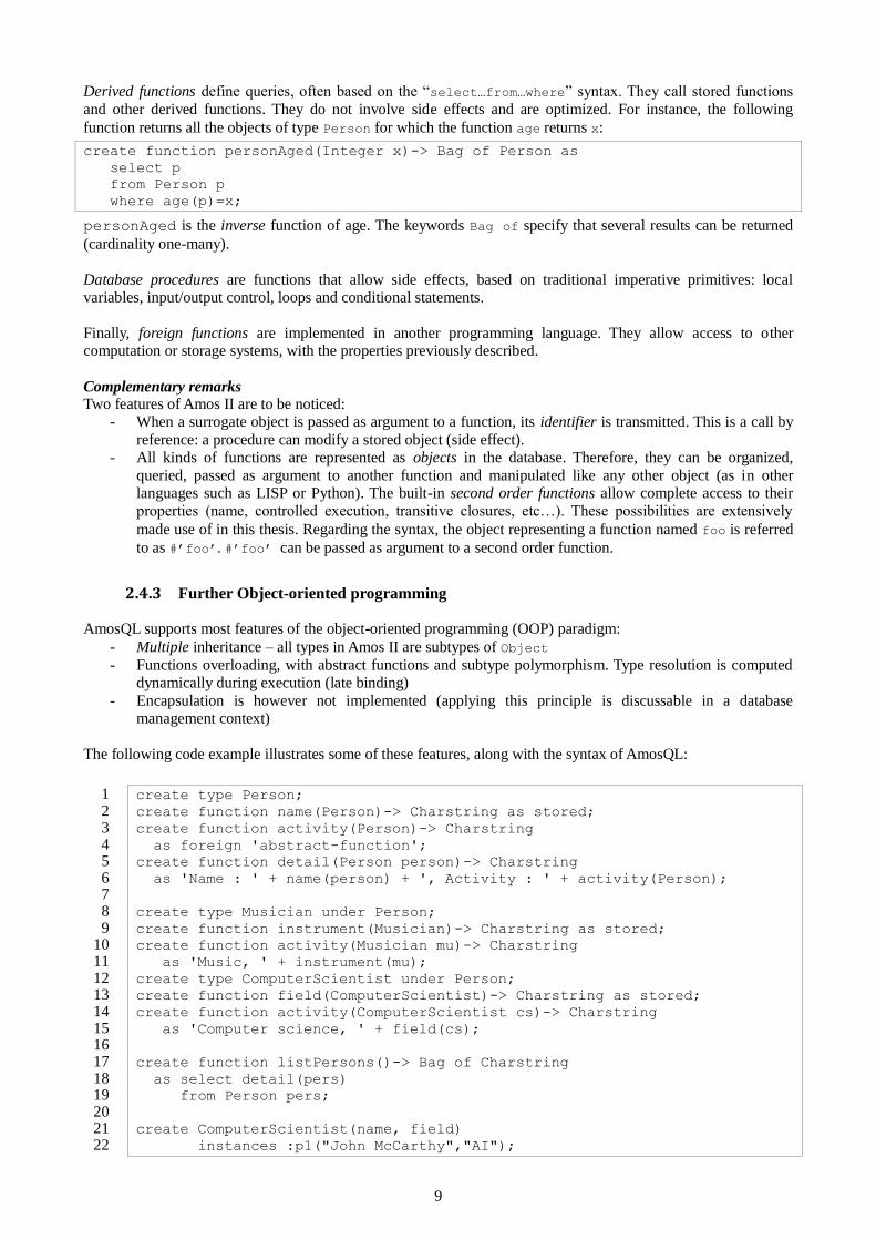
The following code example illustrates some of these features, along with the syntax of AmosQL:
create type Person; 1 create function name(Person)-> Charstring as stored; 2 create function activity(Person)-> Charstring 3 as foreign 'abstract-function'; 4 create function detail(Person person)-> Charstring 5 as 'Name : ' + name(person) + ', Activity : ' + activity(Person); 6 7 create type Musician under Person; 8 create function instrument(Musician)-> Charstring as stored; 9 create function activity(Musician mu)-> Charstring 10 as 'Music, ' + instrument(mu); 11 create type ComputerScientist under Person; 12 create function field(ComputerScientist)-> Charstring as stored; 13 create function activity(ComputerScientist cs)-> Charstring 14 as 'Computer science, ' + field(cs); 15 16 create function listPersons()-> Bag of Charstring 17 as select detail(pers) 18 from Person pers; 19 20 create ComputerScientist(name, field) 21 instances :p1("John McCarthy","AI"); 22
10
create Musician(name, instrument) 23 instances :p2("Oscar Peterson","Piano");24
Figure 2: illustrating OOP with Amos
Lines 1, 8 and 13 create three types: the type Person and its subtypes Musician and ComputerScientist. The
stored function Name, mapping a Person to a Charstring, as well the derived functions activity and detail will be inherited by both subtypes.
The function detail, defined in line 5, returns a string which the concatenation (operator +) of the result of name
and the output of activity for an argument typed Person. The function activity is abstract for Person (lines
3-4), and overridden in Musician (line 10) and ComputerScientist (line 15).
A stored function instrument is declared for Musician as well as a function field for ComputerScientist.
These functions are respectively called by the implementation of activity taking objects typed Musician and
ComputerScientist as argument.
Lines 18 to 20 describe a derived function which calls detail for each object Person in the database.
Finally, lines 22 to lines 25 create an instance :p1 of ComputerScientist for which fields name and field are
populated with “JohnMcCarthy” and “AI”, and an instance :p2 of Musician with name and instrument set to
“Oscar Peterson” and “Piano”.
Calling listPersons(); returns:
"Name : Oscar Peterson, Activity : Music, Piano"
"Name : John McCarthy, Activity : Computer science, AI"
As expected, detail has been called with subtype polymorphism, considering the function activity as it is
defined for the most specific type of its arguments. As said earlier, types are resolved during execution time: this late binding mechanism is central for the work presented in this thesis.
2.4.4 Handling Streams with Amos II
Traditional DBMSs handle static and finite data sets. However, a growing number of applications require dealing with continuous and unbounded data streams [28]. Intuitively, data “passes through” instead of being stored in the
database. The purpose of a Data Stream Management System (DSMS) is to offer generic support for this configuration, along with traditional DBMS functionalities. Although the streamed data is assumed to be structured, applying the traditional SQL operators directly is not sufficient for advanced manipulation. Several
semantics and associated stream query languages have been presented in the past years. Stanford’s CQL [28] is an example of such work. The queries over streams are not only “snapshot” queries, e.g. describing the state of the data at a particular time, but can also be long running: a time varying and unbounded set of results is returned
Amos II has recently been extended to support such functionalities. Among others, the following primitives are
used in this work:
- The type Stream defines precisely what its name suggests. Two snapshots queries over such an object at two different times may return different results.
- The function streamof(Bag)->Stream allows long running queries: its argument (typically, the result of a query) will be continuously evaluated and returned in a stream
- The construct for each [original] [object in stream] [instructions] allows manipulating
each new incoming object. If original is not specified, the manipulations will affect a copy of the
object, which is not suitable for infinite streams.
- The keyword result in stored procedures is quite similar to other language’s return. However, it does
not end the execution of the function. It is therefore possible to yield data, hence producing a stream.
2.5 Learning from data streams
2.5.1 Stream mining and the Incremental Naïve Bayes Classification Framework (INBCF)
Stream mining consists in performing data mining on streamed data. This domain has been extensively studied
11
these last years. Existing classification algorithms have been generalized (such as decision trees, with the Very
Fast Decision Tree algorithm [29]), and new techniques have been developed (for instance, On-Demand Classification[30]). These approaches are motivated by the new constraints imposed by a stream environment:
- Calculations must be performed in one pass - The CPU, and more important, the memory capacities are limited, while the amount of data may be
infinite
- Most assumptions of data mining (the features are distributed independently and identically) do not apply anymore. For instance, the model behind a class may change over time: this is known as the concept drift [31]. The learning algorithm should then be able to “forget the past”, or even adapt its prediction to the
class model as it was at a requested time (under limited memory constraints).
The Incremental Naïve Bayes Classification Framework (INBCF) presented in this thesis allows learning from and classifying streams. Indeed, all computations are realized efficiently in one pass. Nevertheless, it does not fulfill all the previously requirements: it involves a memory usage growing quite fast as the stream feeds the
classifier, and it does not have the ability to “forget”. In this sense, it may be referred to as “pseudo-stream”.
2.5.2 The JSON format
In a streaming context, the INBCF cannot assume that training and testing items are stored in the database. The
JSON (JavaScript Object Notation) standard has been chosen for its simplicity and its popularity as client-server messages format in Web applications.
JSON is a lightweight semi-structured data exchange format [4]. It is currently a standard in Web services, next to XML: commercial organizations such as Yahoo!, Facebook, Twitter and Google use it to deliver some of their feeds. It is language independent, but some platforms support it natively: among others and with different
appellations, PHP, JavaScript, Python, and Amos II (it is equivalent to the type Record).
The following types can be exchanged: number (real or integer), String, Boolean, null, Array and
Object. An Array is an ordered sequence of values; an Object is a collection of key-value pairs. These two types
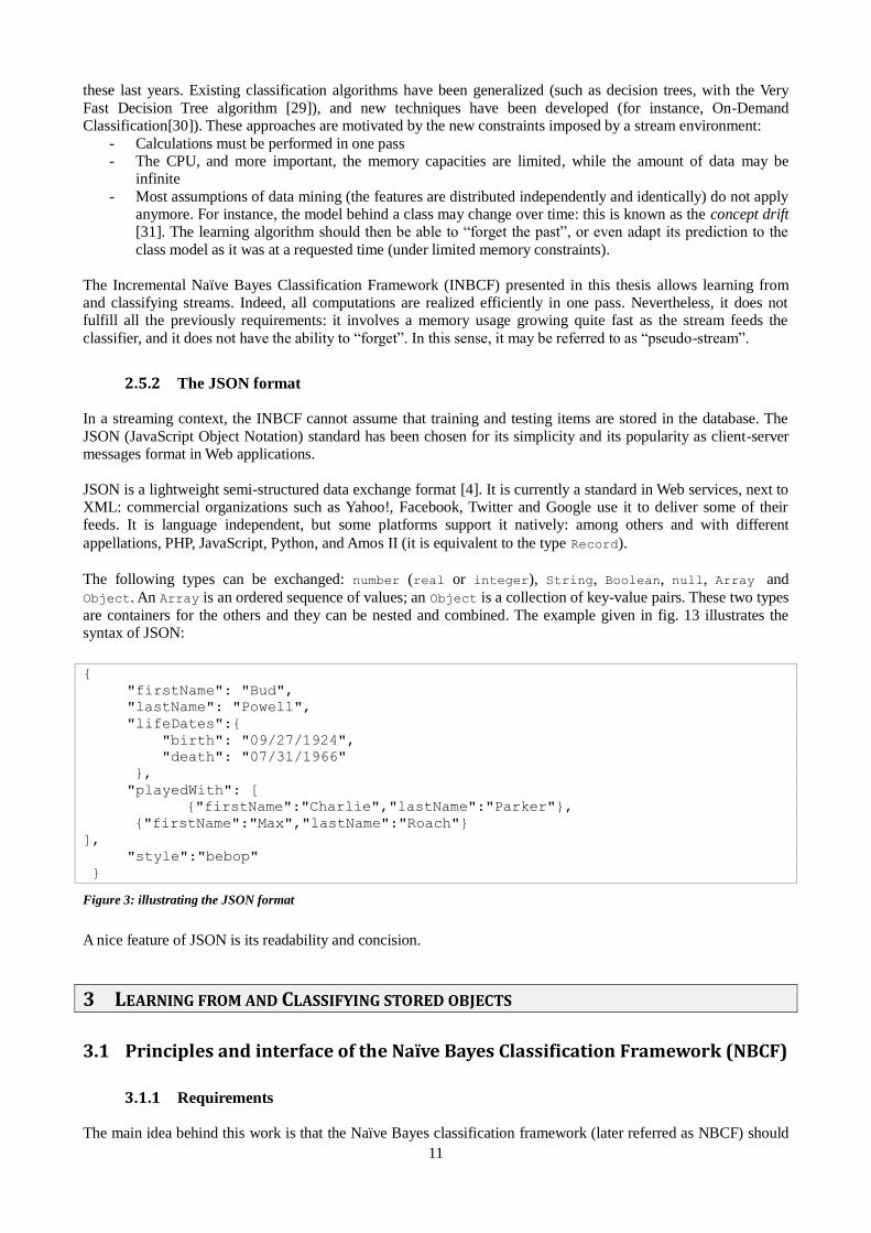
are containers for the others and they can be nested and combined. The example given in fig. 13 illustrates the syntax of JSON:
{
"firstName": "Bud",
"lastName": "Powell",
"lifeDates":{
"birth": "09/27/1924",
"death": "07/31/1966"
},
"playedWith": [
{"firstName":"Charlie","lastName":"Parker"},
{"firstName":"Max","lastName":"Roach"}
],
"style":"bebop"
}
Figure 3: illustrating the JSON format
A nice feature of JSON is its readability and concision.
3 LEARNING FROM AND CLASSIFYING STORED OBJECTS
3.1 Principles and interface of the Naïve Bayes Classification Framework (NBCF)
3.1.1 Requirements
The main idea behind this work is that the Naïve Bayes classification framework (later referred as NBCF) should
12
be fully integrated within the data model of Amos II, in a generic and modular fashion, with respect to the closure
principle (the result of any query can be queried) - During learning and classification phases, objects are directly manipulated along with the functions
defining their features. No conversion to tuple or vector is needed or operated by the NBCF procedures.
With the previously introduced conventions, 𝑋𝑖 is an object (of any type).Then, the user defined functions
(stored or derived) 𝑎𝑡𝑡𝑟1, 𝑎𝑡𝑡𝑟2, 𝑎𝑡𝑡𝑟3…𝑎𝑡𝑡𝑟𝑛 map 𝑋𝑖 to its features 𝑥𝑖1, 𝑥𝑖
2, … , 𝑥𝑖𝑛and 𝑌𝑖 to 𝑦
1, 𝑦2,… , 𝑦𝑛.
These are the feature functions. Similarly, the class to which a training item belongs is defined by a 𝑐𝑙𝑎𝑠𝑠
function returning 𝑐𝑖. The NBCF will directly take the functions 𝑎𝑡𝑡𝑟1, 𝑎𝑡𝑡𝑟2, 𝑎𝑡𝑡𝑟3, … , 𝑎𝑡𝑡𝑟𝑛 and 𝑐𝑙𝑎𝑠𝑠 as argument instead of their result for each training or test item.
- The values of the features or class 𝑥𝑖1, 𝑥𝑖
2, … , 𝑥𝑖𝑛 , 𝑐𝑖of an object can be of any type supporting the equality
(=) operator in Amos II: not only subtypes of Number or Charstring, but also surrogates or interface objects to data stored externally (proxy objects). Therefore, the class object predicted by the classifier can
be directly queried and manipulated - The whole Bayesian model created during the learning phase is completely open: it can be freely queried,
modified, stored and re-used
- The attributes can have different types and assumed to follow different distributions: one type of learning can be specified independently for each attribute. For instance, given an item set, an attribute “weight”
can be modeled by Gaussian distribution, while frequency histograms are generated for a feature “country”. Each of these classification procedures are stored in objects that can be modified or created from scratch by the user. In this sense, the learning is completely modular.
- The NBCF is optimized and particularly lightweight (approx. 500 lines with all components) - The implementation is realized in AmosQL. Everything except the initialization of data structures is
written in a declarative style, with a full use of the included data mining primitives (aggregation, mean,
standard deviation)
3.1.2 Specifications and interface
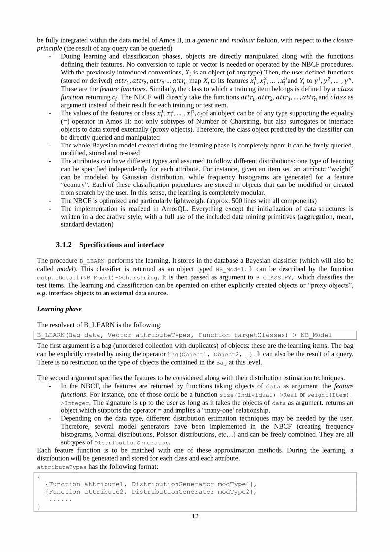
The procedure B_LEARN performs the learning. It stores in the database a Bayesian classifier (which will also be
called model). This classifier is returned as an object typed NB_Model. It can be described by the function
outputDetail(NB_Model)->Charstring. It is then passed as argument to B_CLASSIFY, which classifies the
test items. The learning and classification can be operated on either explicitly created objects or “proxy objects”, e.g. interface objects to an external data source.
Learning phase
The resolvent of B_LEARN is the following:
B_LEARN(Bag data, Vector attributeTypes, Function targetClasses)-> NB_Model
The first argument is a bag (unordered collection with duplicates) of objects: these are the learning items. The bag
can be explicitly created by using the operator bag(Object1, Object2, …). It can also be the result of a query.
There is no restriction on the type of objects the contained in the Bag at this level.
The second argument specifies the features to be considered along with their distribution estimation techniques.
- In the NBCF, the features are returned by functions taking objects of data as argument: the feature
functions. For instance, one of those could be a function size(Individual)->Real or weight(Item)-
>Integer. The signature is up to the user as long as it takes the objects of data as argument, returns an
object which supports the operator = and implies a “many-one’ relationship. - Depending on the data type, different distribution estimation techniques may be needed by the user.
Therefore, several model generators have been implemented in the NBCF (creating frequency histograms, Normal distributions, Poisson distributions, etc…) and can be freely combined. They are all
subtypes of DistributionGenerator.
Each feature function is to be matched with one of these approximation methods. During the learning, a distribution will be generated and stored for each class and each attribute.
attributeTypes has the following format:
{
{Function attribute1, DistributionGenerator modType1},
{Function attribute2, DistributionGenerator modType2},
......
}

13
In Amos II, a Vector is an ordered collection. It is formed with curly brackets.
Finally, the last argument targetClasses is the function which takes the objects of data (the training set) as argument and returns their class: the class function. The signature is up to the user as long as it takes the objects of
data as argument, returns an object which supports the operator = and implies a “many-one’ relationship.
Remark: missing values for a feature are ignored during both learning and classification
Classification phase
The signature for B_CLASSIFY is the following:
B_CLASSIFY(NB_Model model, Bag data)
-> Bag of <Object item, Object class, Real probability>
The first argument is the NB_Model returned by B_LEARN.
The second one, data, is a Bag containing all the objects to be classified. They should have the same type as
the training items.
B_CLASSIFY returns each object of data with their predicted class and the associated probability (more exactly
score, as explained in 3.1.2 (4).
Supported distributions
The implemented distribution generators are described in fig.4. They are subtypes of DistributionGenerator.
Indeed, this type has a function GenerateDistribution which estimates a distribution from a set of observed
values. The function is overridden by each subtype of DistributionGenerator. The implementation is
described in the next section.
Type Learning
Input Generated distribution
Probability
estimation Parameters – Comments
HistogramGenerator Object Frequency histogram Cf. 2.2.4(7)
SmoothHistogramGenerator Object
Smoothened
histogram of
frequencies
Cf. 2.2.4 (8) smoothingStrength : Real
UniformBinGenerator Number Frequency histogram
of binned values Cf. 2.2.4 (7)
nbBins: Integer
nbBins uniform bins are generated
between the observed min and max of
the feature
StdDeviationBinGenerator Number Frequency histogram
of binned values Cf. 2.2.4 (7)
Uniform bins are generated, centered
around the mean with width set to the
observed standard deviation
NormalGenerator Number Normal distribution Cf. 2.2.4 (10)
PoissonGenerator Integer Poisson distribution 𝜇 ��
𝑎𝑘!∙ 𝑒
Figure 4: supported distributions
The first column describes the type of object to be associated with a feature in B_LEARN. The second one specifies
which kind of data (e.g. result of the attribute function) can be handled. The third and fourth columns precise the
type of model to be generated for each class and the estimation method for ��(𝑎𝑘|𝑐). Some DistributionGenerator objects require parameters: these are specified by populating the stored
14
functions presented in the last column. For instance, specifying the strength of smoothing for a
SmoothHistogramGenerator is done by populating the stored function
smoothingStrength(SmoothHistogramGenerator)->Integer with the desired value for the model generator
object. This will be illustrated by the example presented in the following section.
These components all respect a common “interface”. Users can easily create their own distributions and generators. In the implementation, they are organized hierarchically with subtype relationships (for instance,
SmoothHistogramGenerator is a subtype of HistogramGenerator). This will be described in the next section.
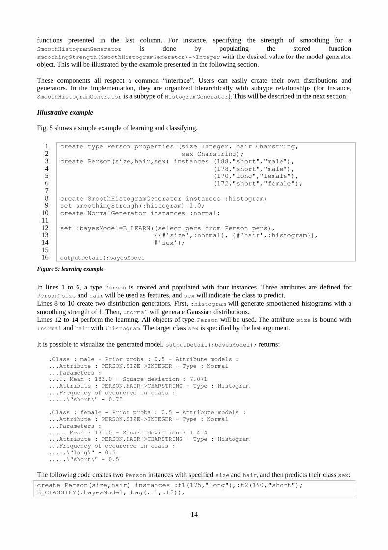
Illustrative example
Fig. 5 shows a simple example of learning and classifying.
create type Person properties (size Integer, hair Charstring, 1 sex Charstring); 2 create Person(size,hair,sex) instances (188,"short","male"), 3 (178,"short","male"), 4 (170,"long","female"), 5 (172,"short","female"); 6 7 create SmoothHistogramGenerator instances :histogram; 8 set smoothingStrengh(:histogram)=1.0; 9 create NormalGenerator instances :normal; 10 11 set :bayesModel=B_LEARN((select pers from Person pers), 12 {{#'size',:normal}, {#'hair',:histogram}}, 13 #'sex‟); 14 15 outputDetail(:bayesModel16
Figure 5: learning example
In lines 1 to 6, a type Person is created and populated with four instances. Three attributes are defined for
Person: size and hair will be used as features, and sex will indicate the class to predict.
Lines 8 to 10 create two distribution generators. First, :histogram will generate smoothened histograms with a
smoothing strength of 1. Then, :normal will generate Gaussian distributions.
Lines 12 to 14 perform the learning. All objects of type Person will be used. The attribute size is bound with
:normal and hair with :histogram. The target class sex is specified by the last argument.
It is possible to visualize the generated model. outputDetail(:bayesModel); returns:
.Class : male - Prior proba : 0.5 - Attribute models :
...Attribute : PERSON.SIZE->INTEGER - Type : Normal
...Parameters :
..... Mean : 183.0 - Square deviation : 7.071
...Attribute : PERSON.HAIR->CHARSTRING - Type : Histogram
...Frequency of occurence in class :
.....\"short\" - 0.75
.Class : female - Prior proba : 0.5 - Attribute models :
...Attribute : PERSON.SIZE->INTEGER - Type : Normal
...Parameters :
..... Mean : 171.0 - Square deviation : 1.414
...Attribute : PERSON.HAIR->CHARSTRING - Type : Histogram
...Frequency of occurence in class :
.....\"long\" - 0.5
.....\"short\" - 0.5
The following code creates two Person instances with specified size and hair, and then predicts their class sex:
create Person(size,hair) instances :t1(175,"long"),:t2(190,"short");
B_CLASSIFY(:bayesModel, bag(:t1,:t2));
15
The statement returns:
<#[OID 1645],"male",0.00371866116410918>
<#[OID 1646],"male",0.0129614036326976>
:t1 and :t2 have been classified as males, with respectively weak and very high probabilities.
3.2 Data structures and algorithms of the NBCF
3.2.1 Structure of the generated Bayesian classifier
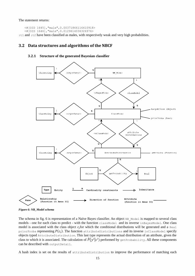
Figure 6: NB_Model schema
The schema in fig. 6 is representation of a Naïve Bayes classifier. An object NB_Model is mapped to several class
models - one for each class to predict - with the function classModel and its inverse inBayesModel. One class
model is associated with the class object 𝑐𝑖for which the conditional distributions will be generated and a Real
priorProba representing 𝑃(𝑐𝑖). The function attributeDistributions and its inverse inClassModel specify
objects typed AttributeDistribution. This last type represents the actual distribution of an attribute, given the
class to which it is associated. The calculation of ��(𝑦𝑖|𝑐𝑖) performed by getProbability. All these components
can be described with outputDetail.
A hash index is set on the results of attributeDistribution to improve the performance of matching each
16
feature with its model in a class.
The calculation of argmax ∈ 𝑃(𝑐) ∙ ∏ 𝑃 (𝑎𝑘 |𝑐 )𝑛𝑘=1 for an item is a simple scan. For each class model, the
logarithms of getProbability for all attributes are summed, and then added to the logarithm of the prior
probability. A “TOP 1” on these results for all classes will return the prediction.
With 𝑛 attributes, |𝐶|classes, and a complexity of probability computation 𝑂(𝑡𝑝 ) of each attributes, the time
complexity for the classification of one item is 𝑂(|𝐶| ∙ (𝑛 ∙ 𝑡𝑝 + 1+ 1)) ≈ 𝑂(|𝐶| ∙ 𝑛 ∙ 𝑡𝑝). This is inherent to an
approach based on the Maximum A Posteriori decision rule.
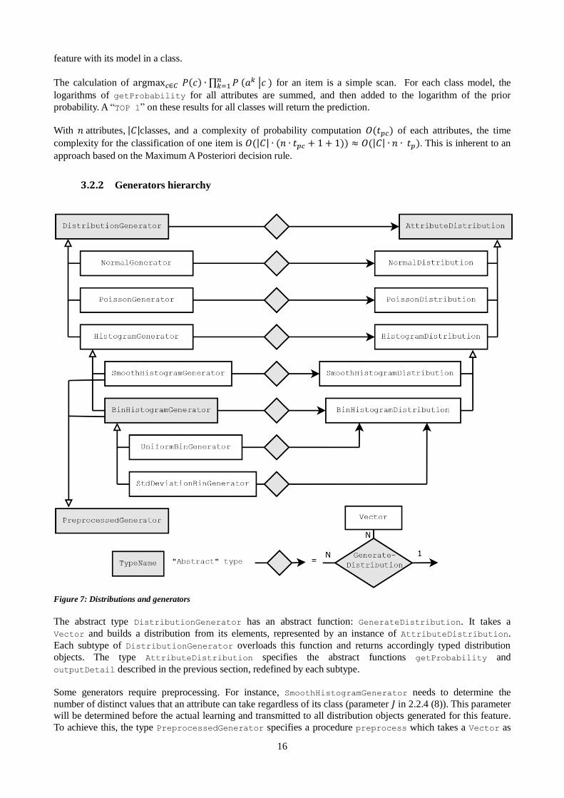
3.2.2 Generators hierarchy
Figure 7: Distributions and generators
The abstract type DistributionGenerator has an abstract function: GenerateDistribution. It takes a
Vector and builds a distribution from its elements, represented by an instance of AttributeDistribution.
Each subtype of DistributionGenerator overloads this function and returns accordingly typed distribution
objects. The type AttributeDistribution specifies the abstract functions getProbability and
outputDetail described in the previous section, redefined by each subtype.
Some generators require preprocessing. For instance, SmoothHistogramGenerator needs to determine the
number of distinct values that an attribute can take regardless of its class (parameter 𝐽 in 2.2.4 (8)). This parameter
will be determined before the actual learning and transmitted to all distribution objects generated for this feature.
To achieve this, the type PreprocessedGenerator specifies a procedure preprocess which takes a Vector as
17
argument and generates the required preprocessing information (not represented in the figure).
Binning operations require preprocessing. A uniform binning system object is generated (and stored) from the
observed values by a method of BinHistogramGenerator. This binning system transforms any continuous value
into a bin object (Vector of two real numbers {Real,Real}), that can be stored, counted and retrieved as any
object by a HistogramDistribution. Once generated, the system will be shared by all distribution objects
describing the concerned feature. Its exact behavior is specified by subtypes of BinHistogramGenerator (for
instance n bins between the minimum of maximum of the learning values, cf. 2.2.4).
A binning system is based on a center 𝑐 and a width 𝑤. For a value v, 𝑏𝑖𝑛𝑣 = *𝑙𝑜𝑤𝑣, 𝑖𝑔𝑣+ will be computed as
follows:
𝑖𝑓 ≥ 𝑐 𝑏𝑖𝑛𝑣 = {𝑙𝑜𝑤𝑣 = 𝑣 − (𝑣 − 𝑐)%𝑤 𝑖𝑔𝑣 = 𝑙𝑜𝑤𝑣 + 𝑤
𝑒𝑙𝑠𝑒 𝑏𝑖𝑛𝑣 = {𝑙𝑜𝑤 = 𝑖𝑔𝑣 − 𝑤
𝑖𝑔𝑣 = 𝑣 − (𝑣 − 𝑐)%𝑤
This is implemented as predicates in a select…from…where clause.
Remark: all types can be instantiated in Amos II. However, some types are based on abstract functions and are only called for inheritance, hence their description as “abstract”.
3.2.3 Learning procedure
The learning is performed in three phases: preprocessing, data organizing and model building.
Preprocessing
The procedure preprocess is called for all PreprocessedGenerators objects. The values of the associated feature for the whole test population are passed as argument.
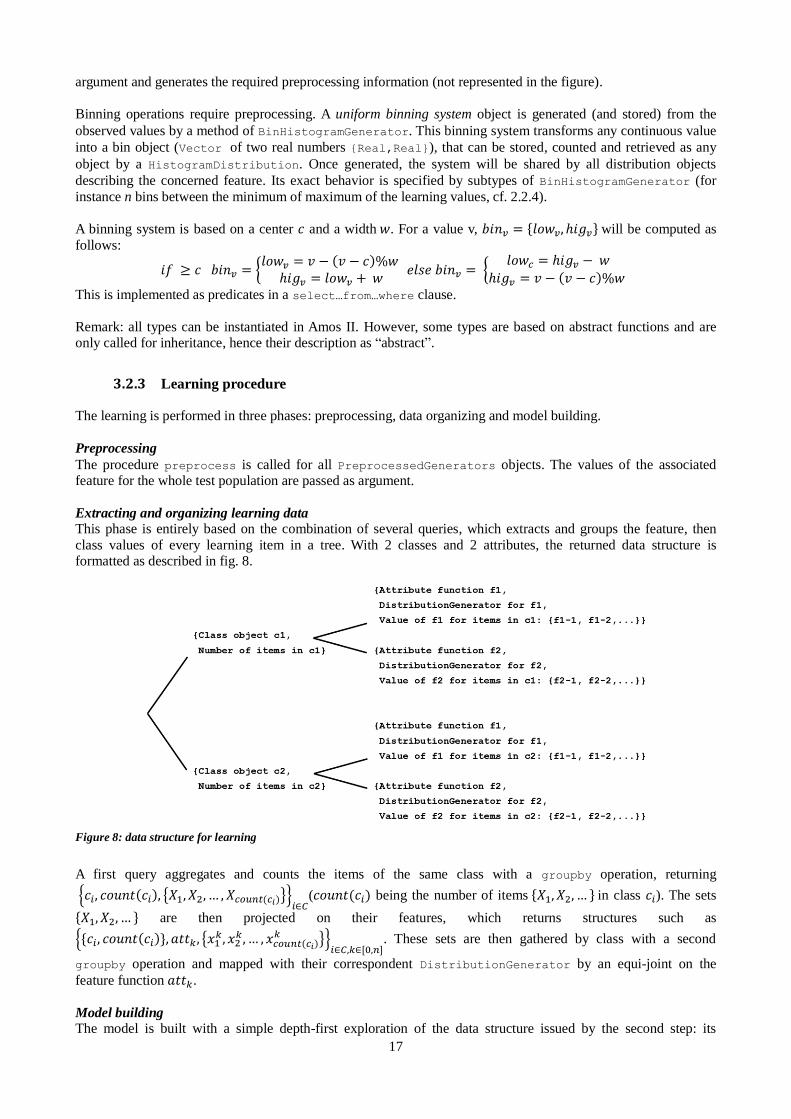
Extracting and organizing learning data This phase is entirely based on the combination of several queries, which extracts and groups the feature, then
class values of every learning item in a tree. With 2 classes and 2 attributes, the returned data structure is formatted as described in fig. 8.
Figure 8: data structure for learning
A first query aggregates and counts the items of the same class with a groupby operation, returning
{𝑐𝑖, 𝑐𝑜𝑢𝑛𝑡(𝑐𝑖), {𝑋1, 𝑋2, … , 𝑋 𝑜𝑢𝑛𝑡( 𝑖)}}𝑖∈ (𝑐𝑜𝑢𝑛𝑡(𝑐𝑖) being the number of items *𝑋1, 𝑋2, … + in class 𝑐𝑖). The sets
*𝑋1, 𝑋2, … + are then projected on their features, which returns structures such as
{*𝑐𝑖, 𝑐𝑜𝑢𝑛𝑡(𝑐𝑖)+, 𝑎𝑡𝑡𝑘, {𝑥1𝑘, 𝑥2
𝑘, … , 𝑥 𝑜𝑢𝑛𝑡( 𝑖)𝑘 }}
𝑖∈ ,𝑘∈, ,𝑛-. These sets are then gathered by class with a second
groupby operation and mapped with their correspondent DistributionGenerator by an equi-joint on the
feature function 𝑎𝑡𝑡𝑘.
Model building The model is built with a simple depth-first exploration of the data structure issued by the second step: its

18
structure matches exactly the schema of NB_Model. For each node of the first level, a ClassModel object is
generated. In each leaf, the function generateDistribution of the DistributionGenerator object is called
with the provided attribute values. The issued distribution object is then attached to the previously generated class model.
With 𝑛 attributes, |𝐶| classes and 𝑝 items, the worst case complexity is the following:
- Given 𝑂(𝑡𝑃𝑃(𝑝)) the number of operations required by the function preprocess, the complexity for the
first phase is: 𝑂(𝑛 ∙ 𝑡𝑝𝑝(𝑝)) - Retrieving classes for p items is done in 𝑂(𝑝) (a hash index is set on the arguments of stored functions by
Amos II). Grouping by class involves 𝑂(𝑝 ∙ |𝐶|) operations. A hash index on the result of the class functions could somehow accelerate this first grouping (this is not implemented by default, it is up to the
user). Extracting all feature values has a complexity of 𝑂(𝑛 ∙ 𝑝). The final grouping is done in 𝑂(|𝐶|𝑛 ∙|𝐶|).
- Therefore, the second step phase on its whole is realized in: 𝑂(𝑝(|𝐶| + 𝑛) + 𝑛|𝐶|2). Nevertheless, in
practice, |𝐶| is very low compared to 𝑛: a complexity of 𝑂(𝑛 ∙ 𝑝) seems like a reasonable evaluation.
- With 𝑂(𝑡𝑚𝑏(𝑝)) the time required to generate a distribution of one feature, the final phase involves
𝑂(|𝐶| + |𝐶| ∙ 𝑛 ∙ 𝑡𝑚𝑏(𝑝)) = 𝑂(|𝐶| ∙ 𝑛 ∙ 𝑡𝑚𝑏(𝑝)) steps.
The “worst” distribution is the smoothened histogram: a first “count distinct” is necessary to count all the values
that an attribute can take regardless of its class during preprocessing. Then, another “count distinct” is involved to generate the frequency histograms for each class. Hash indexes allow these two operations to be performed in
𝑂(𝑝): 𝑡𝑝𝑝 and 𝑡𝑚𝑏 are linear functions. If all features are represented by this distribution and |𝐶| is low, the
overall complexity of learning is 𝑂(𝑛 ∙ (𝑡𝑝𝑝(𝑝) + 𝑝 + 𝑡𝑚𝑏(𝑝)) ) = 𝑂(𝑛 ∙ 𝑝).
3.3 Performance evaluation
3.3.1 Time consumption
To evaluate the NBCF, an alternative architecture has been developed: JavaNB. JavaNB is based on a Java implementation of the Naive Bayes algorithm. All classification and learning tasks involve three steps: retrieving tuples from the database, inserting them in the appropriate data structures, and perform the learning/classification.
The system has the following features:
Normal, histogram and smoothened histogram distributions are supported. It seems reasonable to consider them as representative of all common classification tasks for performance evaluation
the code is optimized, and full use are made of Java's scalable data structures: mostly, HashMap and ArrayList
JavaNB is bound to AmosII via its fastest possible interface: the JavaAmos API [22]
all objects are converted into tuples of String, Integer or Float values. The results of the classification are String objects
The Naive Bayes model is kept in the Java program (not in Amos) JavaNB is optimized but quite poor qualitatively; also its architecture and usage are different from those of the NBCF. Therefore, it is to be considered as a reference point more than a direct competitor.
Both systems were run on the same computer in a mutually exclusive fashion. Data used in this evaluation are synthetic, with the following properties:
Name Default value
Size of the learning item set p 3000
Size of the testing item set 3000
Number of features (n) 15
Number of classes 5
The features will be classified with Normal, Frequency histogram and Smoothened histogram distributions. Each distribution type accounts for 1/3 of the total number of features (10 Normal distribution, 10 Frequency
histograms and 10 Smoothened histograms by default).
19
The categorical values (2/3 of the features) can have 50 distinct values, affected randomly.
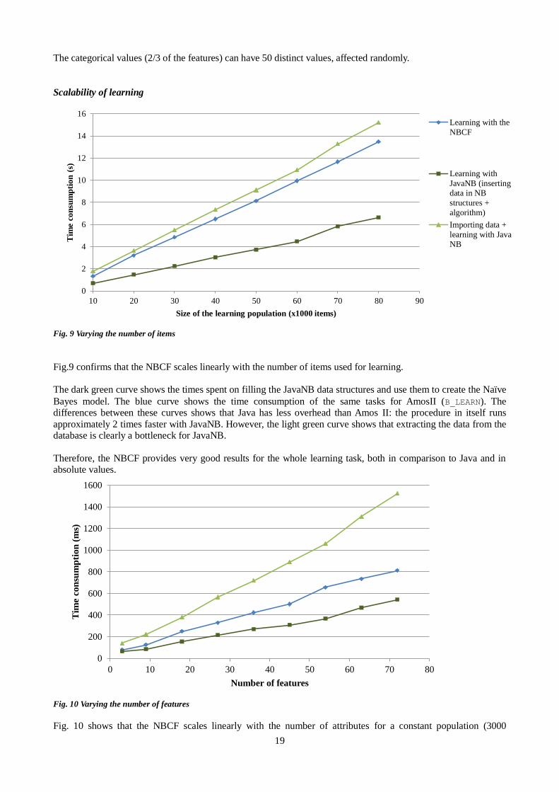
Scalability of learning
Fig. 9 Varying the number of items
Fig.9 confirms that the NBCF scales linearly with the number of items used for learning. The dark green curve shows the times spent on filling the JavaNB data structures and use them to create the Naïve
Bayes model. The blue curve shows the time consumption of the same tasks for AmosII (B_LEARN). The differences between these curves shows that Java has less overhead than Amos II: the procedure in itself runs
approximately 2 times faster with JavaNB. However, the light green curve shows that extracting the data from the database is clearly a bottleneck for JavaNB.
Therefore, the NBCF provides very good results for the whole learning task, both in comparison to Java and in absolute values.
Fig. 10 Varying the number of features
Fig. 10 shows that the NBCF scales linearly with the number of attributes for a constant population (3000
0
2
4
6
8
10
12
14
16
10 20 30 40 50 60 70 80 90
Tim
e co
nsu
mp
tio
n (
s)
Size of the learning population (x1000 items)
Learning with the
NBCF
Learning with
JavaNB (inserting
data in NB
structures +
algorithm)
Importing data +
learning with Java
NB
0
200
400
600
800
1000
1200
1400
1600
0 10 20 30 40 50 60 70 80
Tim
e co
nsu
mp
tion
(m
s)
Number of features
20
individuals). The relative speed difference between JavaNB and the NBCF is not affected by this parameter.
Importing the dataset seems to have a slightly convex behavior; this was confirmed by further experimentations.
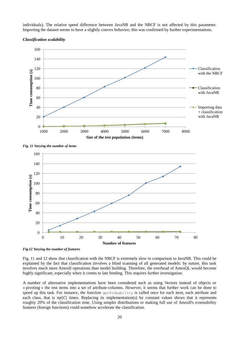
Classification scalability
Fig. 11 Varying the number of items
Fig.12 Varying the number of features
Fig. 11 and 12 show that classification with the NBCF is extremely slow in comparison to JavaNB. This could be explained by the fact that classification involves a blind scanning of all generated models: by nature, this task involves much more AmosII operations than model building. Therefore, the overhead of AmosQL would become
highly significant, especially when it comes to late binding. This requires further investigation.
A number of alternative implementations have been considered such as using Vectors instead of objects or « pivoting » the test items into a set of attribute-columns. However, it seems that further work can be done to
speed up this task. For instance, the function getProbability is called once for each item, each attribute and
each class, that is 𝑛𝑝|𝐶| times. Replacing its implementation(s) by constant values shows that it represents roughly 20% of the classification time. Using simpler distributions or making full use of AmosII's extensibility
features (foreign functions) could somehow accelerate the classification.
0
20
40
60
80
100
120
140
160
1000 2000 3000 4000 5000 6000 7000 8000
Tim
e co
nsu
mp
tion
(s)
Size of the test population (items)
Classification
with the NBCF
Classification
with JavaNB
Importing data
+ classification
with JavaNB
0
20
40
60
80
100
120
140
160
0 10 20 30 40 50 60 70 80
Tim
e co
nsu
mp
tion
(s)
Number of features
21
The time consumption of classification evolves linearly with the number of items and features.
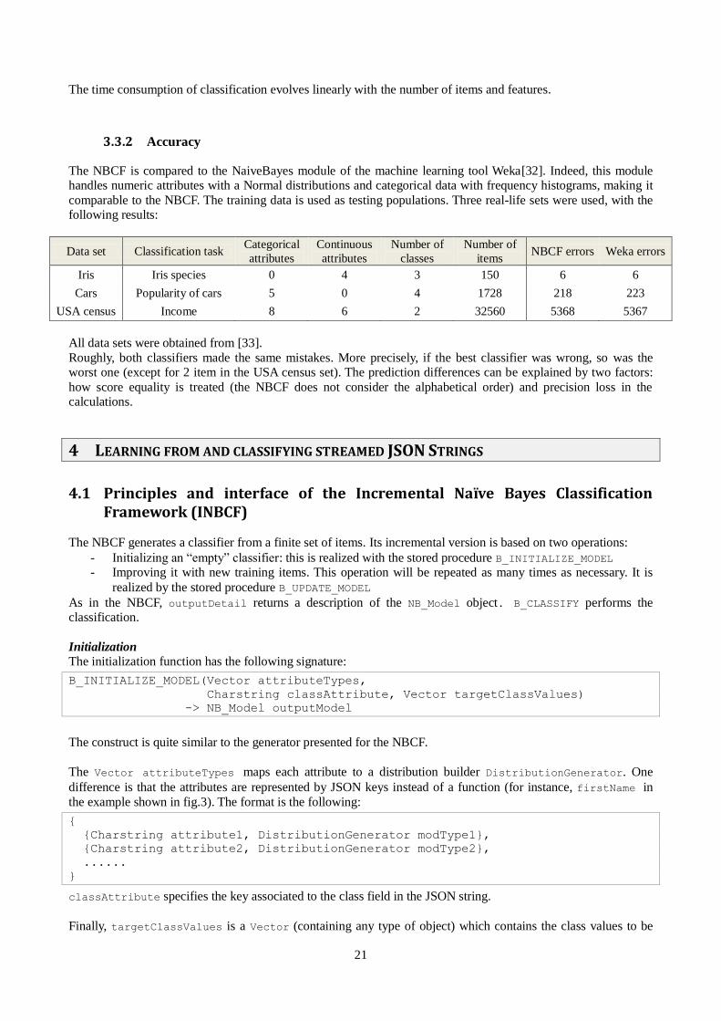
3.3.2 Accuracy
The NBCF is compared to the NaiveBayes module of the machine learning tool Weka[32]. Indeed, this module handles numeric attributes with a Normal distributions and categorical data with frequency histograms, making it
comparable to the NBCF. The training data is used as testing populations. Three real-life sets were used, with the following results:
Data set Classification task Categorical
attributes
Continuous
attributes
Number of
classes
Number of
items NBCF errors Weka errors
Iris Iris species 0 4 3 150 6 6
Cars Popularity of cars 5 0 4 1728 218 223
USA census Income 8 6 2 32560 5368 5367
All data sets were obtained from [33].
Roughly, both classifiers made the same mistakes. More precisely, if the best classifier was wrong, so was the worst one (except for 2 item in the USA census set). The prediction differences can be explained by two factors:
how score equality is treated (the NBCF does not consider the alphabetical order) and precision loss in the calculations.
4 LEARNING FROM AND CLASSIFYING STREAMED JSON STRINGS
4.1 Principles and interface of the Incremental Naïve Bayes Classification Framework (INBCF)
The NBCF generates a classifier from a finite set of items. Its incremental version is based on two operations:
- Initializing an “empty” classifier: this is realized with the stored procedure B_INITIALIZE_MODEL - Improving it with new training items. This operation will be repeated as many times as necessary. It is
realized by the stored procedure B_UPDATE_MODEL
As in the NBCF, outputDetail returns a description of the NB_Model object. B_CLASSIFY performs the classification.
Initialization
The initialization function has the following signature:
B_INITIALIZE_MODEL(Vector attributeTypes,
Charstring classAttribute, Vector targetClassValues)
-> NB_Model outputModel
The construct is quite similar to the generator presented for the NBCF.
The Vector attributeTypes maps each attribute to a distribution builder DistributionGenerator. One
difference is that the attributes are represented by JSON keys instead of a function (for instance, firstName in
the example shown in fig.3). The format is the following:
{
{Charstring attribute1, DistributionGenerator modType1},
{Charstring attribute2, DistributionGenerator modType2},
......
}
classAttribute specifies the key associated to the class field in the JSON string.
Finally, targetClassValues is a Vector (containing any type of object) which contains the class values to be

22
predicted (𝐶 = *𝑐1, 𝑐2, … +). Assuming that the classes are known a priori does not seem unreasonable and allows
nice performance enhancements. Indeed, the updating functions could have detected the new classes as they appeared and build their model “on-the-fly”. However this would have induced a small but significant fixed cost
for each example to be treated.
Learning As one or several JSON strings are received, the Bayesian model can be updated by one of these functions:
B_UPDATE_MODEL(NB_Model bayesModel, Record item)-> Boolean
B_UPDATE_MODEL(NB_Model bayesModel, Vector of Record data)-> Boolean
The first function improves the classifier with a unique JSON String, while the second one is based on a Vector
of JSON String.
These two implementations are separate and independent: passing a Vector of items instead of one object allows
avoiding significant fixed costs. Indeed, the item is not processed as a Vector of one element in the first implementation, nor is the collection of the second scanned with each item being considered separately.
Improving a Naïve Bayes model nbModel with the elements of a stream passing through a function
learnStream() would be handled as follows:
for each original Record item where item in learnStream()
B_UPDATE_MODEL(nbModel, item);
This will run until the function learnStream ends.
Remarks:
- A class or feature value can be of any type that supports the operator = in Amos II, which includes nested
structures (for instance, the value of lifeDates in fig. 3)
- If a feature or class field is in a nested collection (for instance, birth in fig. 13), the JSON string needs to
be “flattened” before feeding the model. This can be easily realized with a derived function in Amos II. - The system runs on a single process: it is blocked while the model is updated or an item is being
classified. Therefore, if the stream contains more items than the classifier can take, it will be sampled.
Classification
A set of test items can be classified with the following function:
B_CLASSIFY(NB_Model model, Vector of Record data)
-> Bag of <Record item, Object class, Real probability>
This function has the same semantic and arguments the one introduced for the NBCF. Alternatively, in the case of binary classification (two classes), the following function can be used:
B_CLASSIFY_BINARY(NB_Model model, Vector of Record data)
-> Bag of <Record item, Object class, Real ratio>
To each predicted class is associated the ratio 𝑝(𝑐1|𝑌𝑖)/𝑝(𝑐2|𝑌𝑖), as explained in 2.2.3 (5). This provides much more interpretable results.
As previously, a for each construct allows classifying streamed items.
Supported distributions All distribution generators described in 3.1.2 are supported, with the following differences:
- The generators StdDeviationBinGenerator and UniformBinGenerator were suppressed. In a streaming context, using a binning system based on observed values (in this case, mean-standard deviation or minimum-maximum) is problematic. Indeed, the bins must remain the same for the whole
stream as the values from which they are inferred change unexpectedly.
- A bin-based distribution generator BinHistogramGenerator was developed (based on the abstract type
of the same name in the NBCF). Its stored function binningParameters (BinHistogramGenerator)
needs to be populated with a Vector {Real center, Real binWidth}. These parameters respectively
specify the width of the bins and value around which they are generated (cf. 3.2.2).
Illustrative example The following example illustrates a simple use case of the INBCF:
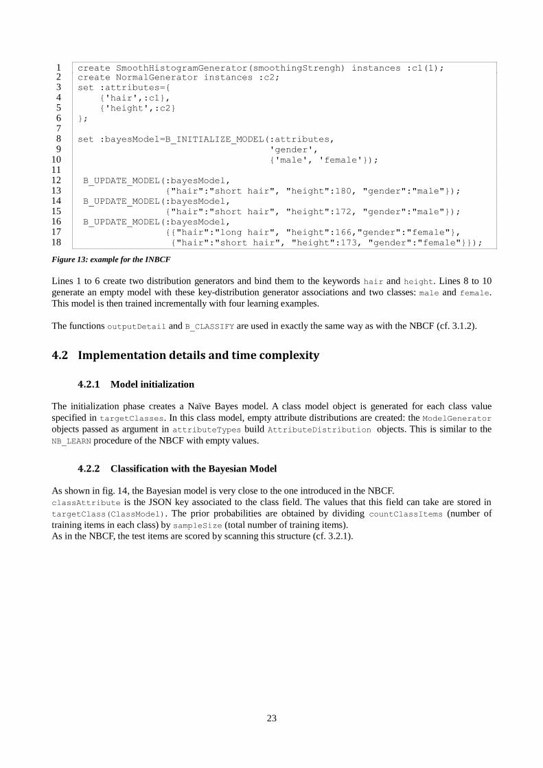
23
create SmoothHistogramGenerator(smoothingStrengh) instances :c1(1); 1 create NormalGenerator instances :c2; 2 set :attributes={ 3 {'hair',:c1}, 4 {'height',:c2} 5 }; 6 7 set :bayesModel=B_INITIALIZE_MODEL(:attributes, 8 'gender', 9 {'male', 'female'}); 10 11 B_UPDATE_MODEL(:bayesModel, 12 {"hair":"short hair", "height":180, "gender":"male"}); 13 B_UPDATE_MODEL(:bayesModel, 14 {"hair":"short hair", "height":172, "gender":"male"}); 15 B_UPDATE_MODEL(:bayesModel, 16 {{"hair":"long hair", "height":166,"gender":"female"}, 17 {"hair":"short hair", "height":173, "gender":"female"}});18
Figure 13: example for the INBCF
Lines 1 to 6 create two distribution generators and bind them to the keywords hair and height. Lines 8 to 10
generate an empty model with these key-distribution generator associations and two classes: male and female.
This model is then trained incrementally with four learning examples.
The functions outputDetail and B_CLASSIFY are used in exactly the same way as with the NBCF (cf. 3.1.2).
4.2 Implementation details and time complexity
4.2.1 Model initialization
The initialization phase creates a Naïve Bayes model. A class model object is generated for each class value
specified in targetClasses. In this class model, empty attribute distributions are created: the ModelGenerator
objects passed as argument in attributeTypes build AttributeDistribution objects. This is similar to the
NB_LEARN procedure of the NBCF with empty values.
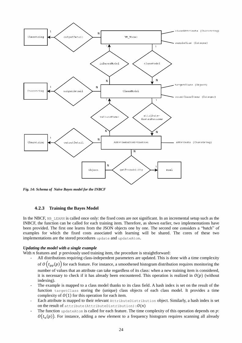
4.2.2 Classification with the Bayesian Model
As shown in fig. 14, the Bayesian model is very close to the one introduced in the NBCF.
classAttribute is the JSON key associated to the class field. The values that this field can take are stored in
targetClass(ClassModel). The prior probabilities are obtained by dividing countClassItems (number of
training items in each class) by sampleSize (total number of training items).
As in the NBCF, the test items are scored by scanning this structure (cf. 3.2.1).
24
Fig. 14: Schema of Naïve Bayes model for the INBCF
4.2.3 Training the Bayes Model
In the NBCF, NB_LEARN is called once only: the fixed costs are not significant. In an incremental setup such as the INBCF, the function can be called for each training item. Therefore, as shown earlier, two implementations have
been provided. The first one learns from the JSON objects one by one. The second one considers a “batch” of examples for which the fixed costs associated with learning will be shared. The cores of these two
implementations are the stored procedures update and updateAtom.
Updating the model with a single example
With 𝑛 features and 𝑝 previously used training item, the procedure is straightforward: - All distributions requiring class-independent parameters are updated. This is done with a time complexity
of 𝑂.𝑡𝑝𝑝(𝑝)/ for each feature. For instance, a smoothened histogram distribution requires monitoring the
number of values that an attribute can take regardless of its class: when a new training item is considered,
it is necessary to check if it has already been encountered. This operation is realized in 𝑂(𝑝) (without
indexing). - The example is mapped to a class model thanks to its class field. A hash index is set on the result of the
function targetClass storing the (unique) class objects of each class model. It provides a time
complexity of 𝑂(1) for this operation for each item.
- Each attribute is mapped to their relevant AttributeDistribution object. Similarly, a hash index is set
on the result of attribute(AttributeDistribution):𝑂(𝑛)
- The function updateAtom is called for each feature. The time complexity of this operation depends on 𝑝:
𝑂(𝑡𝑢(𝑝)). For instance, adding a new element to a frequency histogram requires scanning all already
25
encountered values, which is performed in 𝑂(𝑝) (without indexing).
Therefore, the overall worse case time complexity of a 𝑝𝑡ℎ update operation is 𝑂 (𝑛 ∙ .𝑡𝑝𝑝(𝑝) + 𝑡𝑢(𝑝)/).
In the case where 𝑡𝑝𝑝and 𝑡𝑢 are linear functions, this complexity is 𝑂(𝑛 ∙ 𝑝). In this case, the theoretical total cost
of learning from p items is 𝑂(∑ 𝑖 ∙ 𝑛)𝑝𝑖= = 𝑂 .𝑛 ∙
𝑝(𝑝 1)
2/ = 𝑂(𝑛 ∙ 𝑝2).
In practice, 𝑡𝑝𝑝 and 𝑡𝑢 are constant for all implemented distributions: hash indexing is used to maintain frequency
histograms. Therefore, the total cost required to learn from 𝑝 items is 𝑂(∑ 𝑛𝑃𝑖= ) = 𝑂(𝑝 ∙ 𝑛): the INBCF is
expected to scale similarly to the NBCF.
Updating the model with a batch of examples
The previous approach is generalized for multiple training items. With 𝑛 features, 𝑝 previously used training
items, and a batch of 𝑝’ new items: - All distributions requiring class-independent parameters are updated. The complexity of this operation for
each feature depends on both 𝑝 and 𝑝′: 𝑂.𝑡𝑝𝑝′(𝑝, 𝑝′)/. However, for all implemented distribution types,
𝑂 .𝑡𝑝𝑝′(𝑝, 𝑝′)/ = 𝑂 .𝑝′ ∙ 𝑡𝑝𝑝(𝑝)/. For instance, considering a smoothened frequency histogram, checking
if 𝑝’ values have already been encountered requires 𝑝’ single checks.
- All items are mapped to their matching class model: 𝑂(𝑝′) with a hash index on targetClass
- The features are extracted and mapped with the matching distributions: 𝑂(𝑝′ + 𝑝′ ∙ 𝑛) = 𝑂(𝑝′ ∙ 𝑛)
- The function update is called: 𝑂(𝑡𝑢′ (𝑝, 𝑝′)) = 𝑂(𝑝′ ∙ 𝑡𝑢(𝑝)) for each feature
Updating the model once with 𝑝’ examples has the same asymptotic time consumption that updating the model 𝑝’
times with one example: 𝑂 .𝑛 ∙ 𝑡𝑝𝑝′ (𝑝, 𝑝′) + 𝑝′ + 𝑛 ∙ 𝑝′ + 𝑛 ∙ 𝑡𝑢
′ (𝑝, 𝑝′)/ = 𝑂 .𝑝′ ∙ 𝑛 ∙ (𝑡𝑝𝑝(𝑝) + 𝑡𝑢(𝑝) )/.
Therefore, the total complexity involved in learning from p items is exactly the same as previously. In practice however, evaluation will show that if the algorithm does not scale better than the single item
implementation, it runs much faster: - Fixed costs are spared as the size of the batch grows - Optimization strategies (other than indexing) can be used. Consider for instance the preprocessing
required by a smoothened histogram previously described. 𝑝’ is expected to be much lower than 𝑝, and
these new items are not unique. Therefore, a first “select distinct” is performed on the 𝑝’ incoming items,
which are then aggregated with the previously encountered values of all classes with a “count distinct”.
In other terms, 𝑏 being the batch size, 𝑣(𝑏) the time required to learn from one item, 𝛼 and β two constant factors,
the time required to learn from 𝑝 items with 𝑛 attributes is 𝛼 ∙ 𝑣(𝑏)𝑛𝑝 + 𝛽. Experiments will show that 𝑣(𝑏) decreases drastically with 𝑏.
4.2.4 A close-up on maintained statistics
Generating a frequency histogram with one pass is straight forward. However, approximating some other distributions turned out to be more problematic. For instance, the Gaussian distribution requires incremental
computation of the mean and standard deviation. This section will describe this case.
𝑋 = *𝑥1, 𝑥2, … , 𝑥𝑝+ are the 𝑝 elements that have already been incorporated in the model. The mean and standard
deviation/variance of this population are respectively represented by 𝜇𝑝 and 𝜎𝑝/𝜎𝑝2.
Updating the statistics with one element
An item 𝑥𝑝+1 is appended to 𝑋 = *𝑥1, 𝑥2, … , 𝑥𝑝+ . p, 𝜇𝑝 and 𝜎𝑝2 are assumed to be known.
The task is to compute the mean and variance of 𝑋 ∪ *𝑥𝑝+1+, represented by 𝜇𝑝+1and 𝜎𝑝+12 .
The mean is calculated as follows:
(1) 𝜇𝑝+1 =𝑝 ∙ 𝜇𝑝 + 𝑥𝑝+1
𝑝 + 1
A simple way to monitor the standard deviations is to maintain the sum (∑ 𝑥𝑖2)
𝑝𝑖=1 and use it in:
(2) σp+12 =
1
p + 1∑xi
2
p+1
i=1
− μp+12
In [34], D. Knuth notes that this equation is not numerically stable as it takes the (potentially very small)
26
difference between two large sums. He suggests the following method, discussed and proved in [35]:
With (3) 𝑠𝑝 = 𝑝𝜎𝑝2 = ∑ (𝑥𝑖 − 𝜇𝑝)
2𝑝𝑖=1 assumed to be known:
(4) sp+1 = sp + (xp+1 − μp)(xp+1 − μp+1) with sp+1 = (p + 1)σp+12
(𝑝), (𝜇𝑝) and (𝑠𝑝) are stored and maintained, while (𝜎𝑝) is computed “on demand” for each classification.
Updating the statistics with a batch of elements
A collection of 𝑝′ items 𝑋′ = *𝑥𝑝+1, 𝑥𝑝+2, … , 𝑥𝑝+𝑝′+ with a mean 𝜇𝑝′ and a variance 𝜎𝑝′2 is appended to 𝑋. p, 𝜇𝑝
and 𝜎𝑝2 are assumed to be known. . p’, 𝜇𝑝′ and 𝜎𝑝
2′ are obtained with Amos II’s primitives.
The task is to compute the statistics for 𝑋 ∪ 𝑋′, represented by 𝜇𝑝+𝑝′ and 𝜎𝑝+𝑝′2 .
Indeed, using successively (1) and (3) on each element of 𝑋′ would be satisfying numerically. However, Amos II
contains two primitives vavg(Vector) and vstdev(Vector) returning respectively the mean μ and standard
deviation σ of the elements of a vector. These primitives are very fast, it is therefore preferable to use them. They can be exploited as follows for the mean:
(5) 𝜇𝑝+𝑝′ =𝑝𝜇𝑝 + 𝑝
′𝜇𝑝′
𝑝 + 𝑝′
When it comes to the standard deviation, 𝑠𝑝 defined in (3) is assumed to be known, and 𝑠𝑝′ = ∑ (𝑥𝑖 −𝑝′𝑖=𝑝+1
𝜇𝑝′)2= 𝑝′𝜎𝑝′
2 is directly obtained. Then,
(6) 𝑠𝑝+𝑝′ = 𝑠𝑝 + 𝑠𝑝′ + 𝑝𝑝′
𝑝 + 𝑝′(𝜇𝑝 + 𝜇𝑝′)
2 with sp+p′ = (p + p′)σp+p′
2
As previously, (𝑝), (𝜇𝑝) and (𝑠𝑝) are stored and maintained, while (𝜎𝑝) is computed “on demand” for each
classification. Demonstration:
(6) is obtained by a succession of derivation. A first observation is:
𝑠𝑝 = ∑(xi − μp)2
p
i=1
= ∑𝑥𝑖2
𝑝
𝑖=1
− 2𝜇𝑝 ∑𝑥𝑖
𝑝
𝑖=1
+ 𝑝𝜇𝑝2
= ∑𝑥𝑖2
𝑝
𝑖=1
− 𝑝𝜇𝑝2 (7)
Similarly,
𝑠𝑝′ = ∑ 𝑥𝑖2
𝑝′
𝑖=𝑝+1
− 𝑝′𝜇𝑝′2 ( )
𝑠𝑝+𝑝′ = ∑ 𝑥𝑖2
𝑝+𝑝′
𝑖=1
− (𝑝 + 𝑝′)𝜇𝑝+𝑝′2 ( )
It comes that:
𝑠𝑝+𝑝′ − 𝑠𝑝 = ( ) − (7)
= ∑ 𝑥𝑖2 + 𝑝𝜇𝑝
2 − (𝑝 + 𝑝′)𝜇𝑝+𝑝′2
𝑝′
𝑖=𝑃+1
= 𝑠𝑝′
′ + 𝑝𝜇𝑝2 + 𝑝′𝜇
𝑝′′2 − (𝑝 + 𝑝′)𝜇𝑝+𝑝′
2 with ( )
= 𝑠𝑝′ + 𝑝(𝜇𝑝2 − 𝜇𝑝+𝑝′
2 ) + 𝑝′(𝜇𝑝′2 − 𝜇𝑝+𝑝′
2 )
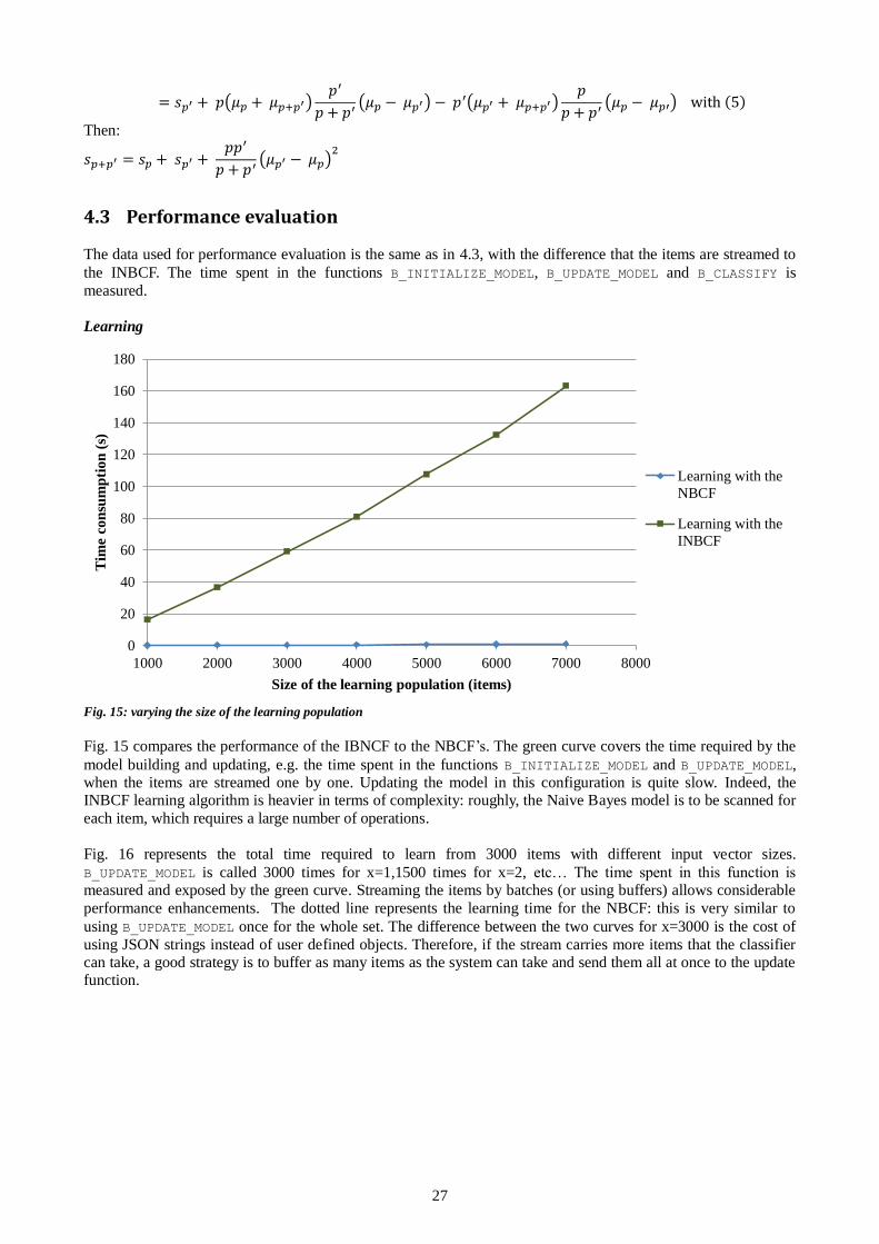
27
= 𝑠𝑝′ + 𝑝(𝜇𝑝 + 𝜇𝑝+𝑝′)𝑝′
𝑝 + 𝑝′(𝜇𝑝 − 𝜇𝑝′) − 𝑝
′(𝜇𝑝′ + 𝜇𝑝+𝑝′)𝑝
𝑝 + 𝑝′(𝜇𝑝 − 𝜇𝑝′) with (5)
Then:
𝑠𝑝+𝑝′ = 𝑠𝑝 + 𝑠𝑝′ + 𝑝𝑝′
𝑝 + 𝑝′(𝜇𝑝′ − 𝜇𝑝)
2
4.3 Performance evaluation
The data used for performance evaluation is the same as in 4.3, with the difference that the items are streamed to
the INBCF. The time spent in the functions B_INITIALIZE_MODEL, B_UPDATE_MODEL and B_CLASSIFY is
measured.
Learning
Fig. 15: varying the size of the learning population
Fig. 15 compares the performance of the IBNCF to the NBCF’s. The green curve covers the time required by the
model building and updating, e.g. the time spent in the functions B_INITIALIZE_MODEL and B_UPDATE_MODEL, when the items are streamed one by one. Updating the model in this configuration is quite slow. Indeed, the INBCF learning algorithm is heavier in terms of complexity: roughly, the Naive Bayes model is to be scanned for
each item, which requires a large number of operations.
Fig. 16 represents the total time required to learn from 3000 items with different input vector sizes.
B_UPDATE_MODEL is called 3000 times for x=1,1500 times for x=2, etc… The time spent in this function is measured and exposed by the green curve. Streaming the items by batches (or using buffers) allows considerable
performance enhancements. The dotted line represents the learning time for the NBCF: this is very similar to
using B_UPDATE_MODEL once for the whole set. The difference between the two curves for x=3000 is the cost of
using JSON strings instead of user defined objects. Therefore, if the stream carries more items that the classifier can take, a good strategy is to buffer as many items as the system can take and send them all at once to the update function.
0
20
40
60
80
100
120
140
160
180
1000 2000 3000 4000 5000 6000 7000 8000
Tim
e co
nsu
mp
tion
(s)
Size of the learning population (items)
Learning with the
NBCF
Learning with the
INBCF
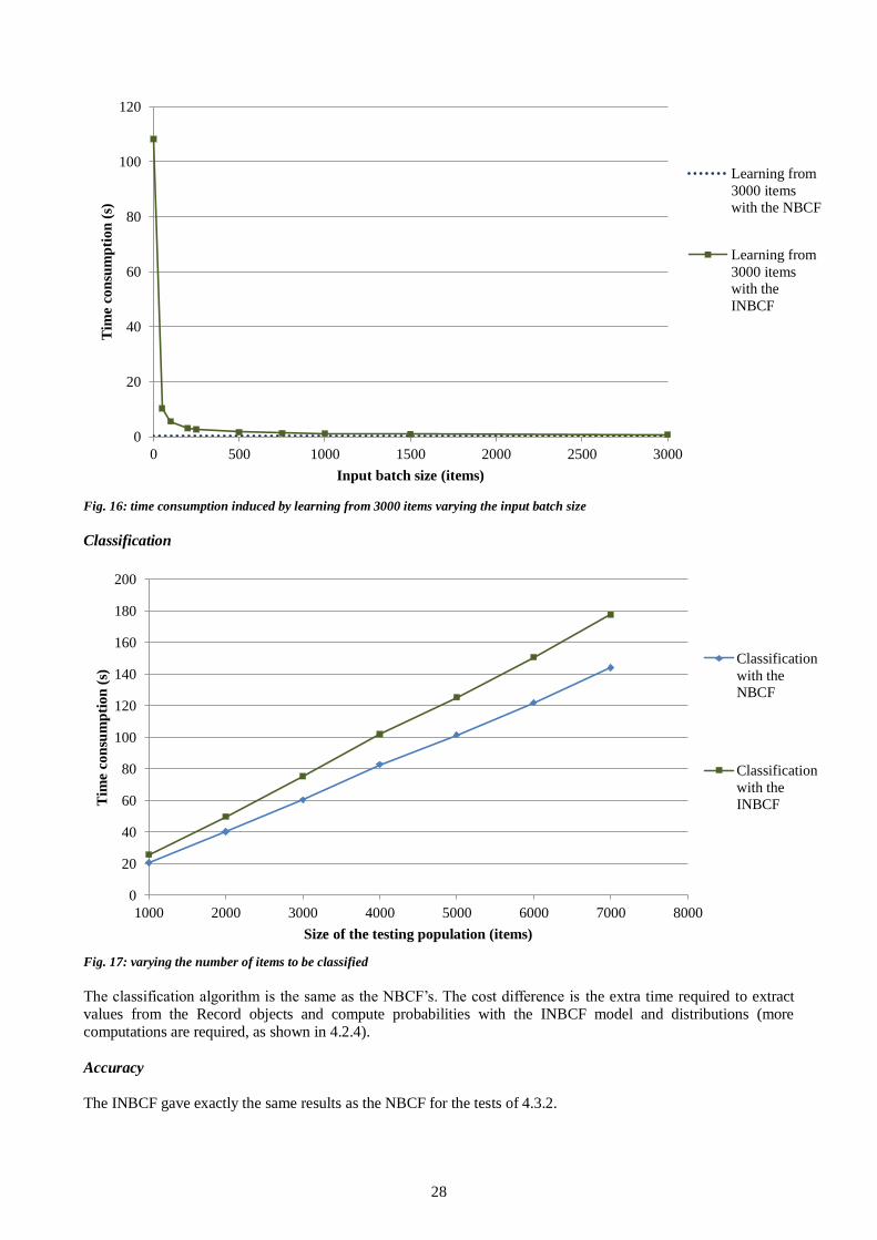
28
Fig. 16: time consumption induced by learning from 3000 items varying the input batch size
Classification
Fig. 17: varying the number of items to be classified
The classification algorithm is the same as the NBCF’s. The cost difference is the extra time required to extract values from the Record objects and compute probabilities with the INBCF model and distributions (more computations are required, as shown in 4.2.4).
Accuracy
The INBCF gave exactly the same results as the NBCF for the tests of 4.3.2.
0
20
40
60
80
100
120
0 500 1000 1500 2000 2500 3000
Tim
e co
nsu
mp
tion
(s)
Input batch size (items)
Learning from
3000 items
with the NBCF
Learning from
3000 items
with the
INBCF
0
20
40
60
80
100
120
140
160
180
200
1000 2000 3000 4000 5000 6000 7000 8000
Tim
e co
nsu
mp
tion
(s)
Size of the testing population (items)
Classification
with the
NBCF
Classification
with the
INBCF

29
5 APPLICATION: CLASSIFYING A STREAM OF MESSAGES DELIVERED BY A SOCIAL NETWORK
5.1 Preliminary notions
5.1.1 Twitter as a source of knowledge
At the time of this work, Twitter is one of the most popular social networks on the Internet. On this website, each user (somehow also contributor) has a personal page on which he would write short messages frequently. The
messages are to contain 140 characters maximum, and deal with any topic. Other users that might be interested in these declarations can subscribe to this page: they will receive a feed each time a new message is written. According to Twitter, approximately 65 million messages would be written each day, by users from all countries.
An interesting feature of this system is the reactivity of its users: any official declaration or important sport event leads to a massive amount of comments in the following minutes. Although its users seem to be mostly young
individuals, numerous organizations use it to broadcast their content (such as CNN or Reuters), as a part of campaign or in advertising plans.
A public API has been published. It allows receiving in quasi-real time a consequent subset of all the messages (there are privacy and commercial-related limitations). Other information is sent along with the text: among others, authors, time, location, spoken language. In terms of machine learning, this is extremely rich data.
This API has been embedded into AmosII [6], allowing to query easily and efficiently this stream of messages. First, a HTTP query specifying some parameters is sent to the Twitter servers. Then the server issues the matching
stream in JSON format.
The following parameters can be specified: - Keywords: up to 200 keywords can be specified. All the returned streams will contain at least one of these
(“or” filter).
- User filter: it is possible to submit a list of users whose messages will be received - Limit: describes the number of messages after which the server will stop emitting
Other access levels allow more parameters (such as longitude-latitude of the user). Nevertheless, they were not
considered for this work.
In the following sections, if not stated otherwise, a keyword filter on “the” is used to obtain (mostly) messages written in English language.
5.1.2 The “bag of words” approach
Text classification is an extremely wide and promising field. However, the purpose of this section is to
demonstrate a usage of the INBCF: an extremely simple approach will be used. The “bag of words” model [36] assumes that considering texts as simple sets of words is acceptable for data mining. The grammar is simply
eluded. This is equivalent to the conditional independence hypothesis of the Naïve Bayes algorithms. Despite this assumption, most techniques based on this model give very good results. In particular, Naïve Bayes is known to be efficient for spam email classification [37].
Many NB text classification techniques and refinements have been proposed. The approach proposed in this thesis
is based on estimating |𝐶| distributions 𝑃(𝑤𝑜𝑟𝑑|𝑐𝑖) and applying the usual decision rules - 3.1.2 (4) and (5). For
instance, classifying 𝑌 with two classes 𝐶 = *𝑠𝑝𝑎𝑚, 𝑛𝑜𝑛 𝑠𝑝𝑎𝑚+ using smoothened histograms is based on
computing:
log 𝑛𝑢𝑚𝑏𝑒𝑟 𝑜𝑓 𝑤𝑜𝑟𝑑𝑠 𝑖𝑛 𝑠𝑝𝑎𝑚 𝑑𝑎𝑡𝑎
𝑛𝑢𝑚𝑏𝑒𝑟 𝑜𝑓 𝑤𝑜𝑟𝑑𝑠 𝑖𝑛 𝑛𝑜𝑛 𝑠𝑝𝑎𝑚 𝑑𝑎𝑡𝑎+∑log
𝑛𝑏. 𝑜𝑓 𝑜𝑐𝑐𝑢𝑟𝑒𝑛𝑐𝑒𝑠 𝑜𝑓 𝑤𝑌 𝑖𝑛 𝑡𝑒 𝑠𝑝𝑎𝑚 𝑑𝑎𝑡𝑎 + 𝑙
𝑛𝑏. 𝑜𝑓 𝑜𝑐𝑐𝑢𝑟𝑒𝑛𝑐𝑒𝑠 𝑜𝑓 𝑤𝑌 𝑖𝑛 𝑡𝑒 𝑛𝑜𝑛 𝑠𝑝𝑎𝑚 𝑑𝑎𝑡𝑎 + 𝑙
𝑡
=1
With a training example 𝑋𝑖 = {{𝑤𝑖1,𝑤𝑖
2, 𝑤𝑖3, … }, 𝑐𝑖}, 𝑤𝑖 being a word and 𝑐𝑖 in 𝐶, the model representing the
probability of occurrence of a word given 𝑐𝑖 will be fed with {𝑤𝑖1, 𝑤𝑖
2,𝑤𝑖3, … }. This is slightly different from the
previous sections: for one training item, many values feed the same model (instead of one model per attribute).
Similarly, classifying a test item 𝑌 = {𝑤𝑌1, 𝑤𝑌
2, 𝑤𝑌3,… ,𝑤𝑦
𝑡} involves comparing log 𝑃(𝑐𝑖) + ∑ log𝑃(𝑤𝑌 |𝑐𝑖)
𝑡 =1 for
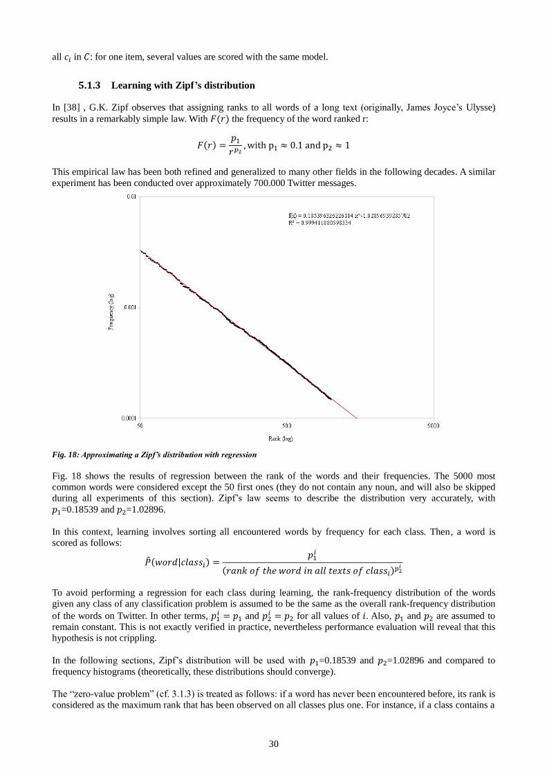
30
all 𝑐𝑖 in 𝐶: for one item, several values are scored with the same model.
5.1.3 Learning with Zipf’s distribution
In [38] , G.K. Zipf observes that assigning ranks to all words of a long text (originally, James Joyce’s Ulysse)
results in a remarkably simple law. With 𝐹(𝑟) the frequency of the word ranked r:
𝐹(𝑟) =𝑝1𝑟𝑝
, with p1 ≈ 0.1 and p2 ≈ 1
This empirical law has been both refined and generalized to many other fields in the following decades. A similar
experiment has been conducted over approximately 700.000 Twitter messages.
Fig. 18: Approximating a Zipf’s distribution with regression
Fig. 18 shows the results of regression between the rank of the words and their frequencies. The 5000 most common words were considered except the 50 first ones (they do not contain any noun, and will also be skipped during all experiments of this section). Zipf’s law seems to describe the distribution very accurately, with
𝑝1=0.18539 and 𝑝2=1.02896.
In this context, learning involves sorting all encountered words by frequency for each class. Then, a word is scored as follows:
��(𝑤𝑜𝑟𝑑|𝑐𝑙𝑎𝑠𝑠𝑖) =𝑝1𝑖
(𝑟𝑎𝑛𝑘 𝑜𝑓 𝑡𝑒 𝑤𝑜𝑟𝑑 𝑖𝑛 𝑎𝑙𝑙 𝑡𝑒𝑥𝑡𝑠 𝑜𝑓 𝑐𝑙𝑎𝑠𝑠𝑖)𝑝 𝑖
To avoid performing a regression for each class during learning, the rank-frequency distribution of the words given any class of any classification problem is assumed to be the same as the overall rank-frequency distribution
of the words on Twitter. In other terms, 𝑝1𝑖 = 𝑝1 and 𝑝2
𝑖 = 𝑝2 for all values of 𝑖. Also, 𝑝1 and 𝑝2 are assumed to remain constant. This is not exactly verified in practice, nevertheless performance evaluation will reveal that this hypothesis is not crippling.
In the following sections, Zipf’s distribution will be used with 𝑝1=0.18539 and 𝑝2=1.02896 and compared to
frequency histograms (theoretically, these distributions should converge).
The “zero-value problem” (cf. 3.1.3) is treated as follows: if a word has never been encountered before, its rank is considered as the maximum rank that has been observed on all classes plus one. For instance, if a class contains a
31
sorted list of 1200 items and another one 1600, it will be 1601.
5.2 Tuning the INBCF
Two changes have been made to the INBCF: Zipf’s distribution has been appended to the original set of models, and a text meta-distribution has been developed.
5.2.1 Zipf’s distribution
Implementing an efficient Zipf’s classifier is non trivial. As described previously, the value which probability is to be computed is neither the word, nor its frequency but its rank compared to all possible other words: this requires maintaining a sorted histogram of all encountered words. The core of the classifier is a stored function
countOccurences()->Bag of <Object value, Integer count>. A hash index is set on value to accelerate
values insertion. A binary index is set on count for sorting operations. Despite the memory consumption of such
practice, the chosen implementation is based on materializing a sorted version of countOccurences into a stored
function valueRanks()->Bag of <Object value, Integer rank>. A hash index is set on value to enhance
retrieving operations. This is realized once at the beginning of B_CLASSIFY: with this configuration, classifying many items at once (e.g. using large input vectors) instead of considering them one by one allows considerable
performance gains.
5.2.2 Wrapper for the distribution of words in a text
It is not possible to classify texts directs with the INBCF as it was described previously: each feature is bound to a
model, whereas text classifications involves using the same model for several values. Therefore, a “meta-model”
has been developed, available through the type TextDistribGenerator. This type wraps a distribution generator
such as those previously described, and it is itself used as any other distribution generator. It tokenizes texts and feeds a distribution with the obtained items.
The following AmosQL example illustrates its usage:
create ZipfGenerator instances :wrapped;
set parameters(:wrapped)={0.18539, 1.028969};
create TextDistribGenerator instances :textGenerator;
set wordsDistribGenerator(:textGenerator)=:wrapped;
set parsingOptions(:textGenerator)={
{" ", ",",":",".","?"},
{"i","a","the","is","have","than","not","do","don't"
{"*:-)*"}
};
create NormalGenerator instances :normalGenerator;
set :classifiers={
{'WorkingHours',:normalGenerator},
{'Conversation',:textGenerator}
};
B_INITIALIZE_MODEL(:classifiers, …)
Fig. 19: calling the text distribution wrapper
The generator :testGenerator will generate a Zipf distribution. However, the functions associated with this distribution will not be called directly: the input will be filtered by the meta-distribution.
For instance, calling getProbability(metaDistribution, “I am”) returns the product of getProbability
(zipfDistribution, “I”) and getProbability(zipfDistribution, “am”). Similarly, calling
updateDistribution(metaDistribution, “I am”) leads to calling successively updateDistribution
(zipfDistribution, “I”) and updateDistribution(zipfDistribution, “am”). All functions of
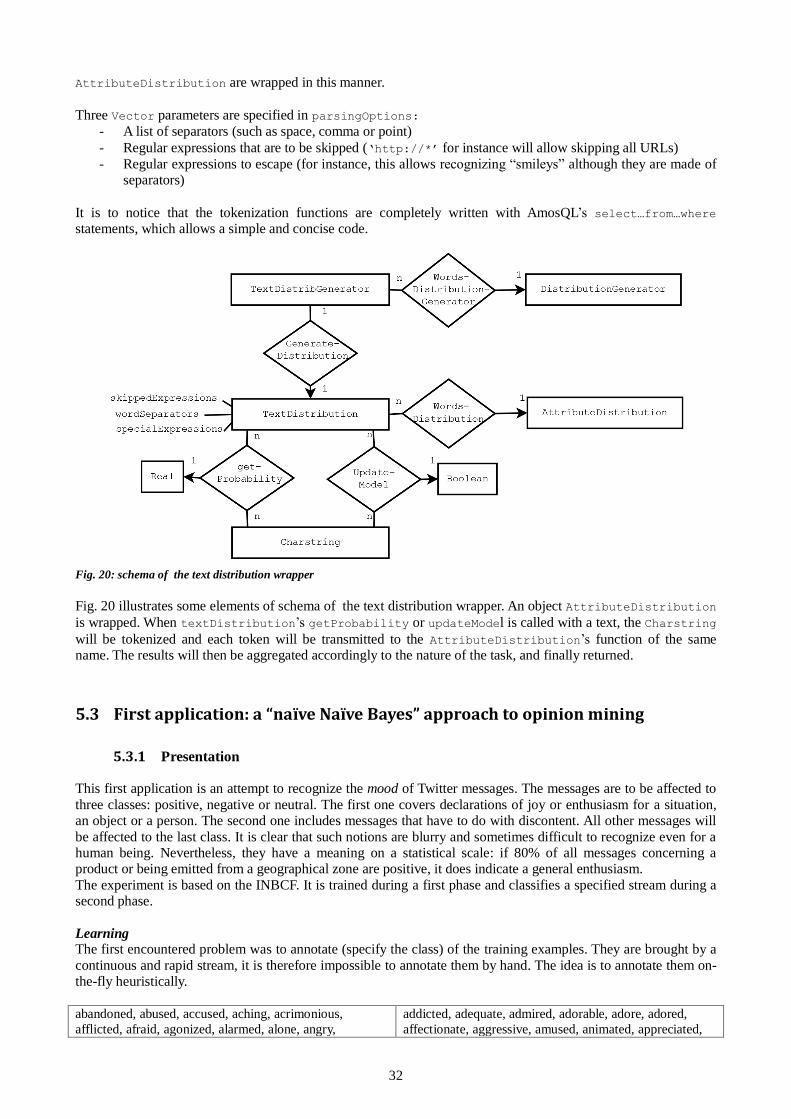
32
AttributeDistribution are wrapped in this manner.
Three Vector parameters are specified in parsingOptions:
- A list of separators (such as space, comma or point)
- Regular expressions that are to be skipped („http://*‟ for instance will allow skipping all URLs)
- Regular expressions to escape (for instance, this allows recognizing “smileys” although they are made of separators)
It is to notice that the tokenization functions are completely written with AmosQL’s select…from…where statements, which allows a simple and concise code.
Fig. 20: schema of the text distribution wrapper
Fig. 20 illustrates some elements of schema of the text distribution wrapper. An object AttributeDistribution
is wrapped. When textDistribution’s getProbability or updateModel is called with a text, the Charstring
will be tokenized and each token will be transmitted to the AttributeDistribution’s function of the same name. The results will then be aggregated accordingly to the nature of the task, and finally returned.
5.3 First application: a “naïve Naïve Bayes” approach to opinion mining
5.3.1 Presentation
This first application is an attempt to recognize the mood of Twitter messages. The messages are to be affected to
three classes: positive, negative or neutral. The first one covers declarations of joy or enthusiasm for a situation, an object or a person. The second one includes messages that have to do with discontent. All other messages will
be affected to the last class. It is clear that such notions are blurry and sometimes difficult to recognize even for a human being. Nevertheless, they have a meaning on a statistical scale: if 80% of all messages concerning a product or being emitted from a geographical zone are positive, it does indicate a general enthusiasm.
The experiment is based on the INBCF. It is trained during a first phase and classifies a specified stream during a second phase.
Learning The first encountered problem was to annotate (specify the class) of the training examples. They are brought by a
continuous and rapid stream, it is therefore impossible to annotate them by hand. The idea is to annotate them on-the-fly heuristically.
abandoned, abused, accused, aching, acrimonious,
afflicted, afraid, agonized, alarmed, alone, angry,
addicted, adequate, admired, adorable, adore, adored,
affectionate, aggressive, amused, animated, appreciated,
33
anguished, annoyed, anxious, appalled, apprehensive,
attacked, baffled, betrayed, bewildered, bitter, blocked,
boiling, cautious…
approved, ardent, aroused, attached, awesome,
enlightened, beatific, blissful, blithe, bright, capable,
captivated, cheerful …
Fig 21. Excerpt from the two word sets
Approximately 150 words expressing positive feelings and 160 words expressing negative feelings have been gathered. Fig. 21 illustrates these lists. Many of these expressions were obtained from [39].
For each message, the number of words which belong to the list of positive (respectively negative) expressions is
counted (including duplicates). Let d be this number. If d>2, the message is marked positive (resp. negative) and it
is repeated 2𝑑 1 times. If the message does not contain any of the listed words, it is marked neutral.
On the whole, some messages will not be annotated correctly: the training set is “noisy”. Nevertheless, the repetition system gives impact to the messages which would be more accurately marked.
Empirical studies reveal that balancing the number of examples so that the prior probabilities are of 1/3 for each
class provides higher classification accuracy. To achieve this, three variables 𝑖, 𝑗 and 𝑘 are maintained. If 𝑖>0,
positive examples are accepted. They are rejected otherwise. 𝑗 and 𝑘 have the same role for negative and neutral
examples respectively. Each time a positive example feeds the model, 𝑖 is decremented and 𝑗 incremented.
Negatives examples have similar effects on 𝑗 and 𝑘, and neutral messages for 𝑘 and 𝑖. For instance, initializing 𝑖 with 10 and the other variables with 0 will release 10 tokens. These tokens will spread circularly between the three classes. To avoid losses, a (limited) buffer stores all messages that were rejected, and injects them again as soon as their matching classes are available.
A list of the 80 most common words on Twitter has been established. Experimentations revealed that skipping
them during learning and classification improved accuracy.
Classification
Once the model built, it can be used to classify any set or stream of JSON feeds. Interesting experiments may be made with Twitter’s filters. For instance the latitude-longitude filter could allow comparing the “moods” of different regions of the world (the output of such experiment would naturally to be discussed). Specifying
keywords could give clues about the reception of a product by its customers (the same remark applies).
A nice feature is that the model can be queried: for instance the name Avatar (a recently released movie) comes as 1224
th in the encountered “positive” words, while it does not appear in the negative words.
5.3.2 Accuracy evaluation
Two sets of 500 raw items each were obtained from Twitter. The first one contains messages filtered by the
keyword “weather”. The second one is based on the word “life”. The motivation behind these choices is to use general topics on which users would express opinions. They were annotated manually by three persons, with a
majority rule in case of conflict. The accuracy is measured by the Kappa statistic between these “experts” and the INBCF.
Two setups are compared: the first one is based on a smoothened frequency histogram, the second one on Zipf’s distribution. Training time was varied, which provides the 12 following classifiers:
Training time Number of messages used for training
Zipf's distribution
based classifier
Frequency histograms
based classifier
12min 1184 zipf1 his1
47min 4318 zipf2 his2
1h35 8624 zipf3 his3
2h15 12583 zipf4 his4
3h01 17693 zipf5 his5
3h30 21603 zipf6 his6
Fig. 22: 12 classifiers to recognize basic emotions

34
The same portion of the training stream was used to generate the two kinds of classifiers.
“Weather” set
Fig. 23: comparing distributions on the “weather” data set
The results of the experiments with the messages containing the word “weather” are exposed in fig. 23. - Except for zipf2 and his2, the classifier based on Zipf’s distribution provides more accurate results. This
would imply that the real ranks are learnt before the real frequencies. Such effect might however be due to the training data. The distributions are expected to converge with further training.
- The difference between zipf2 and his2 reveal that frequency histograms are more accurate with a very small training set. Indeed, according to Zipf’s law, a few words are very common and most of the others are rare. In other words, high frequencies are very high and low frequencies are very low. Therefore, the
lack of precision of the frequency histogram is “exaggerated”. - Both curves have the same general behavior: when accuracy rises for one classifier, it also rises for the
other one. However there is a flat zone between his4 and his5, while the Kappa statistic for the Zipf
classifier grows. To explain this, it seems reasonable to consider three sets of training words. The first set would cover the very frequent words (as said earlier, the less meaningful ones were skipped), which
distribution is assumed to be steady. As they occur often, their modeling converges rapidly. After a certain time, learning from them does not improve the accuracy of the classifier anymore. The flat zone suggests that this phenomenon occurs between 10,000 and 15,000 messages. Remain the less common words, for
which training is longer. If they are contained in the testing set, encountering them will provide better results. Then, both curves rise. If not, they will have a different impact according to the chosen distribution type. Changing the rank of a word can an impact on many other words in Zipf’s distribution:
the relative occurrence frequencies are considered. Therefore, even if the words met during a learning
perio𝑑 𝑇𝑛 do not concern the test examples, they will have an impact on the rank of the testing words that
were encountered in the previous perio𝑑𝑠 𝑇𝑛 1, 𝑇𝑛 2... Oppositely, the part of the frequency histogram involved in the test does not change.
The following table gives the detail of Zipf6’s errors.
INBCF predictions
Negative Neutral Positive
Human
annotation
Negative 40 26 20 17%
Misclassifications: 105
Neutral 22 265 14 59%
Kappa: 0,63
Positive 4 19 101 24%
Accuracy: 79%
13% 61% 26% 511
0,2
0,25
0,3
0,35
0,4
0,45
0,5
0,55
0,6
0,65
0,7
0 5000 10000 15000 20000 25000
Kap
pa s
tati
stic
Number of messages used for training
Zipf
classification
Smoothened
histogram
classification
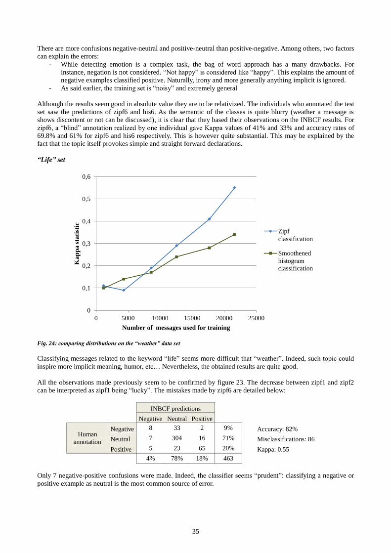
35
There are more confusions negative-neutral and positive-neutral than positive-negative. Among others, two factors can explain the errors:
- While detecting emotion is a complex task, the bag of word approach has a many drawbacks. For instance, negation is not considered. “Not happy” is considered like “happy”. This explains the amount of negative examples classified positive. Naturally, irony and more generally anything implicit is ignored.
- As said earlier, the training set is “noisy” and extremely general Although the results seem good in absolute value they are to be relativized. The individuals who annotated the test
set saw the predictions of zipf6 and his6. As the semantic of the classes is quite blurry (weather a message is shows discontent or not can be discussed), it is clear that they based their observations on the INBCF results. For
zipf6, a “blind” annotation realized by one individual gave Kappa values of 41% and 33% and accuracy rates of 69.8% and 61% for zipf6 and his6 respectively. This is however quite substantial. This may be explained by the fact that the topic itself provokes simple and straight forward declarations.
“Life” set
Fig. 24: comparing distributions on the “weather” data set
Classifying messages related to the keyword “life” seems more difficult that “weather”. Indeed, such topic could
inspire more implicit meaning, humor, etc… Nevertheless, the obtained results are quite good.
All the observations made previously seem to be confirmed by figure 23. The decrease between zipf1 and zipf2 can be interpreted as zipf1 being “lucky”. The mistakes made by zipf6 are detailed below:
INBCF predictions
Negative Neutral Positive
Human
annotation
Negative 8 33 2 9%
Accuracy: 82%
Neutral 7 304 16 71%
Misclassifications: 86
Positive 5 23 65 20%
Kappa: 0.55
4% 78% 18% 463
Only 7 negative-positive confusions were made. Indeed, the classifier seems “prudent”: classifying a negative or
positive example as neutral is the most common source of error.
0
0,1
0,2
0,3
0,4
0,5
0,6
0 5000 10000 15000 20000 25000
Kap
pa s
tati
stic
Number of messages used for training
Zipf
classification
Smoothened
histogram
classification

36
5.4 Second application: a NB-enhanced keyword filter
5.4.1 Principles
The method previously described (learning with heuristic annotation) is generalized into a keyword filter. Indeed, the vocation of the OR filter proposed by Twitter is not accuracy and a simple AND filter would be too restrictive.
Intuitively, the idea is to recognize the words which come up frequently when keywords are associated. For instance, “apple” would often be associated with “steve jobs”, whereas it would less likely come up with “steve” and “jobs” separately.
The filter is implemented as a function, with the following resolvent:
searchTwitter(Vector of Charstring keywords, Integer nbLearningFeeds,
Charstring login, Charstring password)
-> Stream of Record
keywords specifies the words to be searched (more than one). nbLearningFeeds is the number of messages used
to train the filter (in practice, many messages will be skipped in order to keep 0.5 prior priorities). login and
password are the Twitter user account information.
The filter is trained during a first phase. It is based on Zipf’s distribution. Two classes are considered: positive
(relevant) and negative. The Twitter query is a OR filter on the keywords, with a limit set to nbLearningFeeds
messages. The items are annotated heuristically. Let 𝑑 be the number of covered keywords (including duplicates).
If 𝑑 = 1, the message is considered as “negative”. If 𝑑 > 1, it is considered as “positive” and will be repeated
3𝑑 1 times. Experiments showed that skipping the keywords when learning from the texts gives better accuracy. The filtering and buffering system presented in the last section is used to keep 0.5 priors.
Once the classification phase is terminated, the same stream is classified and JSON objects marked negative are
skipped. A nice strategy is to run a AND filter on the top of the system. The filters would then be triggered as
follows: OR ∧ (INBCF ∨ AND)
5.4.2 Accuracy evaluation
Query:”white”, “house”, “Washington” The model/filter is trained with 5 disjoint sets of different sizes, then run on a set of 501 Twitter. These words are very independent semantically. However, their association produces a non ambiguous meaning. Therefore, a good
accuracy is expected. The test texts were annotated manually. They are marked positive if they deal directly with the American government. For instance, “Obama’s policy” is accepted. “The Washington Post” is marked negative.
Fig. 25: results for “white”, “house” and “Washington”
0
0,1
0,2
0,3
0,4
0,5
0,6
0,7
0,8
0,9
0 10000 20000 30000 40000 50000 60000
Number of training messages
Precision
Recall
Accuracy
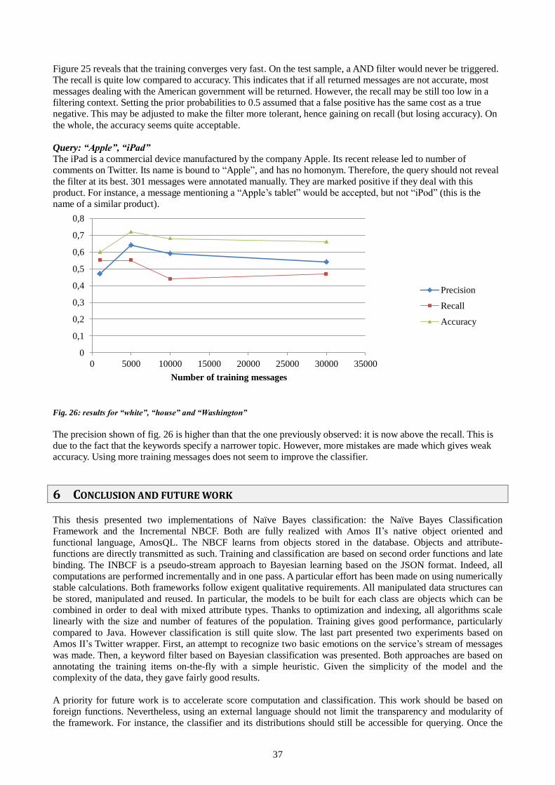
37
Figure 25 reveals that the training converges very fast. On the test sample, a AND filter would never be triggered. The recall is quite low compared to accuracy. This indicates that if all returned messages are not accurate, most
messages dealing with the American government will be returned. However, the recall may be still too low in a filtering context. Setting the prior probabilities to 0.5 assumed that a false positive has the same cost as a true negative. This may be adjusted to make the filter more tolerant, hence gaining on recall (but losing accuracy). On
the whole, the accuracy seems quite acceptable.
Query: “Apple”, “iPad”
The iPad is a commercial device manufactured by the company Apple. Its recent release led to number of comments on Twitter. Its name is bound to “Apple”, and has no homonym. Therefore, the query should not reveal
the filter at its best. 301 messages were annotated manually. They are marked positive if they deal with this product. For instance, a message mentioning a “Apple’s tablet” would be accepted, but not “iPod” (this is the name of a similar product).
Fig. 26: results for “white”, “house” and “Washington”
The precision shown of fig. 26 is higher than that the one previously observed: it is now above the recall. This is due to the fact that the keywords specify a narrower topic. However, more mistakes are made which gives weak accuracy. Using more training messages does not seem to improve the classifier.
6 CONCLUSION AND FUTURE WORK This thesis presented two implementations of Naïve Bayes classification: the Naïve Bayes Classification Framework and the Incremental NBCF. Both are fully realized with Amos II’s native object oriented and
functional language, AmosQL. The NBCF learns from objects stored in the database. Objects and attribute-functions are directly transmitted as such. Training and classification are based on second order functions and late
binding. The INBCF is a pseudo-stream approach to Bayesian learning based on the JSON format. Indeed, all computations are performed incrementally and in one pass. A particular effort has been made on using numerically stable calculations. Both frameworks follow exigent qualitative requirements. All manipulated data structures can
be stored, manipulated and reused. In particular, the models to be built for each class are objects which can be combined in order to deal with mixed attribute types. Thanks to optimization and indexing, all algorithms scale linearly with the size and number of features of the population. Training gives good performance, particularly
compared to Java. However classification is still quite slow. The last part presented two experiments based on Amos II’s Twitter wrapper. First, an attempt to recognize two basic emotions on the service’s stream of messages
was made. Then, a keyword filter based on Bayesian classification was presented. Both approaches are based on annotating the training items on-the-fly with a simple heuristic. Given the simplicity of the model and the complexity of the data, they gave fairly good results.
A priority for future work is to accelerate score computation and classification. This work should be based on foreign functions. Nevertheless, using an external language should not limit the transparency and modularity of
the framework. For instance, the classifier and its distributions should still be accessible for querying. Once the
0
0,1
0,2
0,3
0,4
0,5
0,6
0,7
0,8
0 5000 10000 15000 20000 25000 30000 35000
Number of training messages
Precision
Recall
Accuracy
38
classifier accelerated, the INBCF should be developed to fully handle streams. First, this involves being able to
detect concept drifts or supporting windows and forgets non relevant old training examples. Methods have been proposed to maintain frequency histograms and statistics in this context. They could be used to adjust the class
models over time. Then, the focus could be set on limiting memory consumption, using data summaries. Finally the accuracy of the classifier could be improved by combining it with incremental K-Means.
7 BIBLIOGRAPHY
[1] Tore Risch, Vanja Josifovski, and Timour Katchaounov, "Distributed, Functional Data Integration in a Distributed Mediator System," Functional Approach to Computing with Data, Springer, 2004.
[2] Harry Zhang, "The Optimality of Naive Bayes," in 17th FLAIRS Confernce, 2004.
[3] Carlos Ordonez and Sasi K. Pitchamalai, "Bayesian Classifiers Programmed in SQL," IEEE, pp. 139-144,
January 2010.
[4] (2010, July) Introducing JSON. [Online]. http://www.json.org/
[5] Twitter. [Online]. www.twitter.com
[6] Yang Bo, "Querying JSON Streams," Uppsala University, MSc Thesis IT 10 030, 2010.
[7] G. Piatetsky-Shapiro and W. J. Frawley, Knowledge Discovery in Databases, AAAI/MIT Press, Ed., 1991.
[8] Surajit Chaudhuri, "Data Mining and Database Systems: Where is the Intersection?," Data Engineering
Bulletin, no. 21, 1998.
[9] Tomasz Imielinskiand and Heikki Mannila, "A Database Perspective on Knowledge Discovery," Communications of the ACM, vol. 39, November 1996.
[10] Rakesh Agrawal and Kyuseok Shim, "Developing Tightly-Coupled Data Mining Applications on a Relational Database System," in 2nd Int'l Conference on Knowledge Discovery in Databases and Data Mining, 1996.
[11] D. J. Hand, Heikki Mannila, and Padhraic Smyth, Principles of data mining, MIT Press, Ed., 2001.
[12] Jim Gray, "Data Cube: A Relational Aggregation Operator Generalizing Group-By, Cross-Tab, and Sub Totals," Data Mining and Knowledge Discovery, vol. 1, no. 1, pp. 29-53, 1997.
[13] Meo R., P. Giuseppe, and Ceri S., "A new SQL-like Operator for Mining Association Rules," in Proc. of VLDB96, Mumbai, India, 1996.
[14] T. Imielinski and A. Virmani., "MSQL: A query langugage for database mining," Data Mining and
Knowledge Discovery, vol. 3, no. 4, pp. 373–408, 1999.
[15] J. Han, Y. Fu, W. Wang, K. Koperski, and O. Zaiane, "DMQL: a data mining query language for relational
databases," in Proc. ACM SIG-MOD Workshop DMKD'96, Montreal, Canada, 1996.
[16] Tom Mitchell, Machine Learning, McGraw Hill, Ed., 1997.
[17] George H. John and Pat Langley, "Estimating Continuous Distributions in Bayesian Classifiers," in
Proceedings of the eleventh conference on Uncertainty in Artificial Intelligence, San Mateo, 1995.
[18] Landis JR and Koch GG., "The measurement of observer agreement for catergorical data," Biometrics, vol. 33, pp. 159-74, 1977.
[19] S. Thomas and M.M. Campos, "SQL-Based Naive Bayes Model Building and Scoring," 7,051,037, 2006.
[20] Martin Hansson, Vanja Josifovski, Timour Katchaounov, Tore Risch, Martin Sköld, and Erik Zeitler Staffan
Flodin, Amos II Release 12 User's Manual., 2010.
[21] Tore Risch, "Amos II External Interfaces," Uppsala University, UDBL Technical Report, Dept. of Information Technology 2001.
[22] D. Elin and T. Risch, "Amos II Java Interfaces," UDBL Technical Report, Dept. of Information Technology 2000.
[23] Hanzheng Zou, "Python Integration with a Functional DBMS," Uppsala University, MSc Thesis, Department
of Information Technology IT 09 036, 2009.
[24] C. Werner, "PHP Integration with object relational DBMS," Uppsala University, MSc Thesis, UBDL, Dept. of information technology.
[25] T. Katchaounov, T. Risch, and S. Zürcher, "Object-Oriented Mediator Queries to Internet Search Engines," in International Workshop on Efficient Web-based Information Systems (EWIS), Montpellier, France, 2002.
[26] M.Nyström and T.Risch, "Optimising Mediator Queries to Distributed Engieering Systems," in Proc. 9th International Conference on Database Systems for Advanced Applications (DASFAA 2004), Jeju Island,

39
Korea, 2004.
[27] D. Shipman, "The Functional Data Model and the Data Language DAPLEX," ACM Transactions on
Database Systems, vol. 6(1), 1981.
[28] Arvind Arasu et al., "STREAM: The Stanford Data Stream Management System," Department of Computer Science, Stanford University, 2004.
[29] P. Domingos and G.Hullen, "Mining High-Speed Data Streams," in Proceedings of the 6th ACM SIGKDD conference, Boston, USA, 2000, pp. 71-80.
[30] Charu C. Aggrawal, Jiawey Han Jianyong, and Philip S. Yu, "On-Demand Classification of Data Streams," in KDD'04, Seattle, USA, 2004.
[31] Widmer G. and Kubat M., "Learning in the presence of concept drift and hidden contexts," Machine
Learning, no. 23, pp. pp. 69-101, 1996.
[32] (2010) http://www.cs.waikato.ac.nz/ml/weka/.
[33] (2010) UCI machine learning repository. [Online]. http://archive.ics.uci.edu/ml/index.html
[34] Donald E. Knuth., Volume 2 of The Art of Computer Programming, Seminumerical Algorithms, Addison-Wesley ed. Boston, 1998.
[35] Tony Finch, "Incremental calculation of weighted mean and variance," University of Cambridge, 2009.
[36] David Lewis, "Naive (Bayes) at Forty: The Independence Assumption in Information Retrieval," in Proceedings of ECML-98, 10th European Conference on Machine Learning, Heidelberg, 1998, pp. 4–15.
[37] M. Shahami, S. Dumais, D. Heckermann, and E. Horovitz, "A Bayesian approach to filtering junk e-mail," in AAAI'98 Workshop on Learning for Text Categorization , 1998.
[38] G. K. Zipf, The Psych-biology of Language: an Introduction to Dynamic Philology.: Houghton Mifflin
Company, 1935.
[39] The Compass DeRose Guide to Emotion Words. [Online].
http://www.derose.net/steve/resources/emotionwords/ewords.html
[40] W.Litwin and T.Risch, "Main Memory Oriented Optimization of OO Queries Using Typed Datalog with Foreign Predicates," IEEE Transactions on Knowledge and Data Engineering, vol. 4, no. 6, December 1992.
[41] Giedrius Povilavicius, "A JDBC Driver for an Object-Oriented Database Mediator," Uppsala University, Master's Thesis in Computing Science ISSN 1100-1836, 2005.
[42] Marcus Eriksson, "An ODBC Driver for the mediator database AMOS II ," Linköping Studies in Science and
Technology, Master's Thesis LiTH-IDA-Ex-99/50, 1999.