241

29

Emergy Analysis of a Sucessional Agroforestry System (SAF)

Teldes Corrêa Albuquerque, Enrique Ortega Rodríguez

and Victor Salek Bosso

ABSTRACT

This research aims to study the recovery of a degraded area through the establishment of an

agroforestry system (AFS) at Catavento farm, located in Indaiatuba County, state of Sao Paulo, Brazil,

to demonstrate both the economic and ecological viability of AFS for small farmers. It was studied: (a)

the ecosystem's behavior using emergy (H. T. Odum, 1996); (b) a species consortium with vegetable

succession and nutrients cycling. A data survey has been done on soil covering, classification of

species and identification of their ecological and economic functions and their life cycles. By applying

the mentioned methodologies, a prediction of the agroforestry system behavior and a diagnosis of the

dynamic process of ecological restoration have been carried out, using emergy indicators calculated

for a complete cycle of forest recovery (fifty years). The emergy indices obtained were: Transformity

(Tr), Renewability (%R), Emergy Yield Ratio (EYR), Emergy Investment Ratio (EIR) and Emergy

Exchange Ratio (EER). The following values were found: Transformity varies from 8000 and 12000

seJ/J; Renewability starts at 52% and reaches 81% in the third year, and then grows slowly up to 93%

in 50 years. The initial value of EYR is 2; it reaches 6.5 in 10 years and 13 in 50years. The EIR varies

from 0.17 at the start and after 40 years it decreases to 0.10, showing that the economic investment is

low. The EER value is 1.0 at the beginning, it decreases rapidly (0.2 in year 4), then decreases slowly

(minimum value of 0.1 in 40 years) showing a slight recovery (up to 0.2 in year 50). The annual profit

has been calculated for the cases of both a farm with employees and family managed farm. In the

employer-employee case, the profitability is negative in the first 4 years; in the year 5, the profit is

$550/ha.year, goes up to US $ 900/ha.year in year 6 and reaches a maximum at year 40 (US$

17.000/ha.year).

INTRODUCTION

Large-scale agricultural production systems with intensive use of agrochemicals and machinery

have been questioned for not preserving biodiversity, soil and water quality. Thus, new alternatives for

agricultural production need to be studied and implemented to recover agro-ecosystems quality

through ecological farming techniques, among which agroforestry systems stand out.

In Albuquerque’s research of on agro-silvopastoral systems (SASPs) (2006), some questions were

raised for future studies, both related to SASPs and agroforestry systems (SAFs). In order to continue

this research, contacts were a made to identify an ecological farm located in Indaiatuba County near to

the city of Campinas (São Paulo State) that could be useful as case study. The Catavento farm was

chosen the farm owner was willing to provide information of the agroforestry system under

development. The concepts of systemic interpretation of rural production units were presented to the

farm owner, Mr. Fernando Ataliba, as well as the possibility of applying the emergy analysis on the

area where a SAF is being implemented. The landowner already knew the emergy methodology since

it had been applied by Albuquerque (2006) to the Nata da Serra Farm in Serra Negra (São Paulo State).

The farmer agreed with the study of the small area (one hectare) where he is implementing an

242

agroforestry system since 2006. The landowner had previously visited the Association of Agroforestry

Farmers (COOPERA-FLORESTA) in Barra do Turvo (Sao Paulo State), and recognized the positive

results of agroforestry. The main research lines of the project were traced along with the producer, who

was willing to offer all the information, in order to obtain the following data along time: (a) total

biomass, organic matter and soil nutrients, (b) carbon sequestered, (c) wood and fruits production. In

this research, the emergy methodology was slightly modified to be able to analyze an agroforestry

system, which differs from others for presenting the following characteristics: food production along

tree's growth, different periods of production of all species and different species growing rates in the

different steps of the agroforestry development. In the conventional emergy calculation only inputs and

outputs are used, whereas in the agroforestry systems the changes in the internal stocks were accounted

based on calculations of Roncon (2012).

LITERATURE REVIEW

The SAFs represent an alternative, on a sustainable and economic basis, for family farmers,

considering the forest management, product diversity, and income generation (COSTA, 2008).

Agroforestry Systems are defined as “land management where trees or shrubs are used in association

with crops and/or animals, in the same area, simultaneously or in a temporal sequence”. The function

of crop fertilizing promoted by trees and shrubs, justifies the use of SAFs (LUNDGREN, 1887;

OLIVEIRA e SCHREINER 1987; DUBOIS et al., 1996; MANUAL AGROFLORESTAL, 2008).

According to Oliveira (2009), Agroforestry Systems emerge as an alternative for environmental and

socio-economic development, which seeks to benefit the production system through the enrichment of

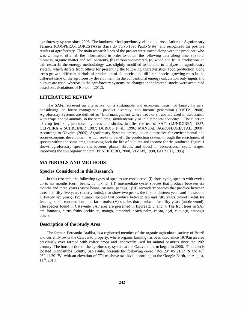
species within the same area, increasing both the life of cultures and income for the producer. Figure 1

shows agroforestry species (herbaceous plants, shrubs, and trees) in successional cyclic stages,

improving the soil organic content (PENEIREIRO, 2008, VIVAN, 1998, GOTSCH, 1995).

MATERIALS AND METHODS

Species Considered in this Research

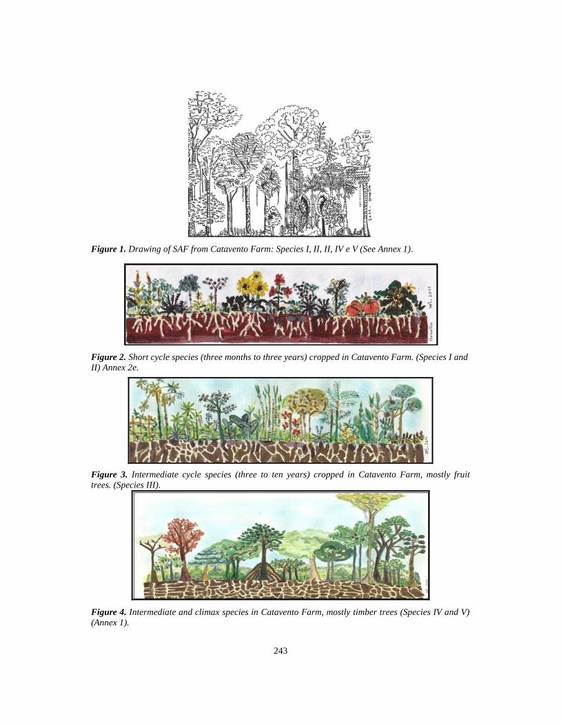
In this research, the following types of species are considered: (I) short cycle, species with cycles

up to six months (corn, beans, pumpkins); (II) intermediate cycle, species that produce between six

months and three years (castor beans, cassava, papaya); (III) secondary: species that produce between

three and fifty five years (mostly fruits), that show two peaks, the first at thirteen years and the second

at twenty six years; (IV) climax: species that produce between ten and fifty years (wood useful for

fencing, small constructions and farm tools; (V) species that produce after fifty years (noble wood).

The species found in Catavento SAF area are presented in figures 2, 3, and 4. The fruit trees in SAF

are: bananas, citrus fruits, jackfruits, mango, tamarind, peach palm, cacao, açaí, cupuaçu, amongst

others.

Description of the Study Area

The farmer, Fernando Ataliba, is a registered member of the organic agriculture society of Brazil

and currently owns the Catavento property, where organic farming has been used since 1979.in an area

previously over farmed with coffee crops and incorrectly used for animal pastures since the 19th

century. The introduction of the agroforestry system at the Catavento farm began in 2006. The farm is

located in Indaituba County, Sao Paulo, presents the following coordinates 23° 05’21.83’’S and 47°

05’ 11.20’’W, with an elevation of 774 m above sea level according to the Google Earth, in August,

11th

, 2010.

243

Figure 1. Drawing of SAF from Catavento Farm: Species I, II, II, IV e V (See Annex 1).

Figure 2. Short cycle species (three months to three years) cropped in Catavento Farm. (Species I and

II) Annex 2e.

Figure 3. Intermediate cycle species (three to ten years) cropped in Catavento Farm, mostly fruit

trees. (Species III).

Figure 4. Intermediate and climax species in Catavento Farm, mostly timber trees (Species IV and V)

(Annex 1).

244

Emergy Methodology for SAFs Analysis

Emergy analysis

Emergy is all the available energy of one kind that is used up, directly and indirectly, in the

transformation processes needed to make a product or a service. Sunlight, fuel, electricity, and human

service can be converted on a common basis by expressing them in the emjoules of solar energy

required in their production. The value is of a unit of emergy is expressed in solar emjoules

(abbreviated seJ). Although other units have been used, such as coal emjoules or oil emjoules, this

research expresses all its emergy data in solar emjoules. Emergy accompanying a flow of something

(energy, matter, information, etc.) is easily calculated if the emergy per unit value is known. The flow

expressed in its usual units is multiplied by the emergy per unit of that flow. For example, the flow of

fuels in Joules per time can be multiplied by the transformity of that fuel (solar emjoules/Joule). A

flow of emergy per unit of time is named empower (Odum, 2000).

Conventional, productive and agroecological agriculture models

According to Ortega (2002), chemical agriculture is usually perceived as a black box, meaning a

closed system in which interactions with the environment are not taken into account and a linear

response in production is expected, it is not the case of emergy analysis of complex agricultural

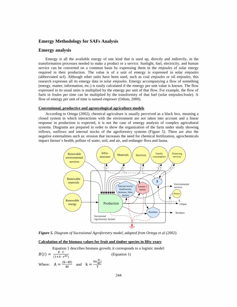
systems. Diagrams are prepared in order to show the organization of the farm under study showing

inflows, outflows and internal stocks of the agroforestry systems (Figure 5). There are also the

negative externalities such as: erosion that increases the need for chemical fertilization, agrochemicals

impact farmer’s health, pollute of water, soil, and air, and endanger flora and fauna.

Figure 5. Diagram of Sucessional Agroforestry model, adapted from Ortega et al (2002).

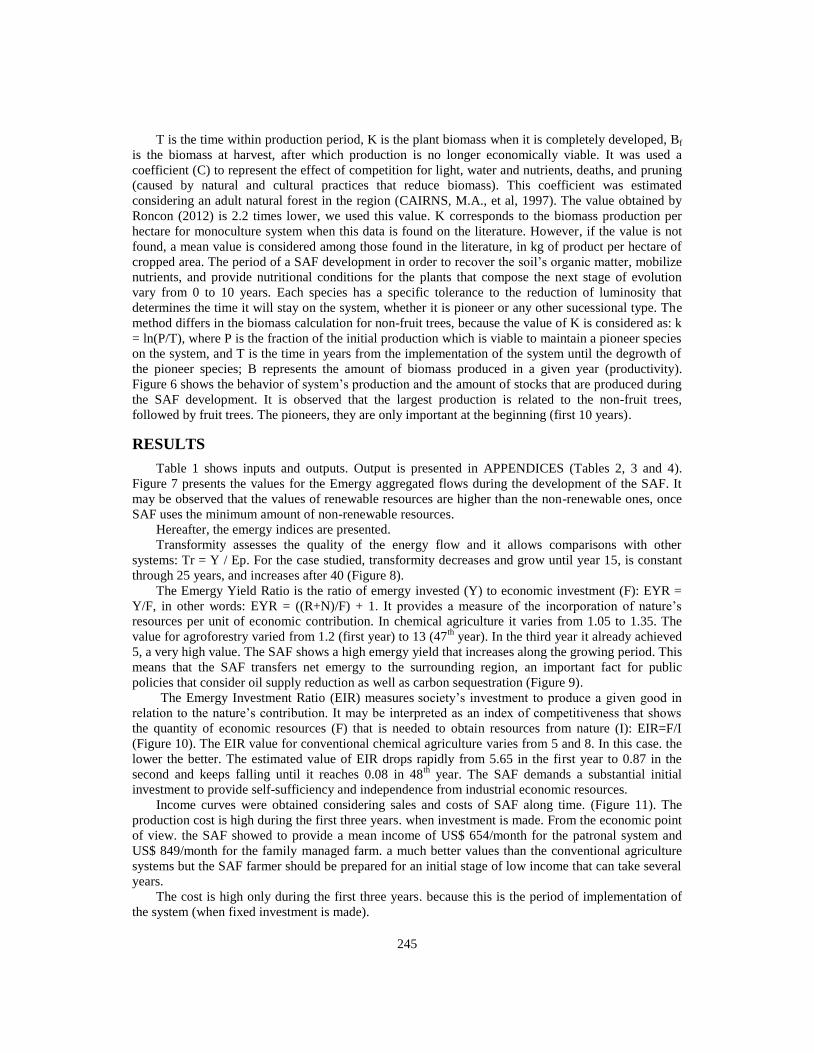
Calculation of the biomass values for fruit and timber species in fifty years

Equation 1 describes biomass growth; it corresponds to a logistic model:

( )

( ) (Equation 1)

Where: ( )

and

(

)

Renewable

energy Production

Renewable

materials

Infra-

structureMaterials Services

Internal stocks:

biodiversity,

biomass, litter,

humus

$

Farmer´s

family

Family

consumption

Sucessional

Agroforestry System

Output

$

Prices

Residues

Renewable

environmental

services

Residues

Environmental

services

Financing

services

245

T is the time within production period, K is the plant biomass when it is completely developed, Bf

is the biomass at harvest, after which production is no longer economically viable. It was used a

coefficient (C) to represent the effect of competition for light, water and nutrients, deaths, and pruning

(caused by natural and cultural practices that reduce biomass). This coefficient was estimated

considering an adult natural forest in the region (CAIRNS, M.A., et al, 1997). The value obtained by

Roncon (2012) is 2.2 times lower, we used this value. K corresponds to the biomass production per

hectare for monoculture system when this data is found on the literature. However, if the value is not

found, a mean value is considered among those found in the literature, in kg of product per hectare of

cropped area. The period of a SAF development in order to recover the soil’s organic matter, mobilize

nutrients, and provide nutritional conditions for the plants that compose the next stage of evolution

vary from 0 to 10 years. Each species has a specific tolerance to the reduction of luminosity that

determines the time it will stay on the system, whether it is pioneer or any other sucessional type. The

method differs in the biomass calculation for non-fruit trees, because the value of K is considered as: k

= ln(P/T), where P is the fraction of the initial production which is viable to maintain a pioneer species

on the system, and T is the time in years from the implementation of the system until the degrowth of

the pioneer species; B represents the amount of biomass produced in a given year (productivity).

Figure 6 shows the behavior of system’s production and the amount of stocks that are produced during

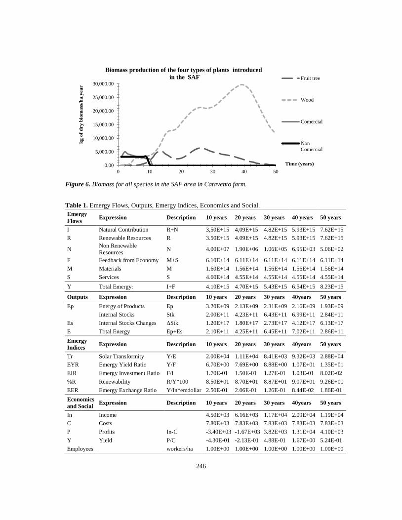
the SAF development. It is observed that the largest production is related to the non-fruit trees,

followed by fruit trees. The pioneers, they are only important at the beginning (first 10 years).

RESULTS

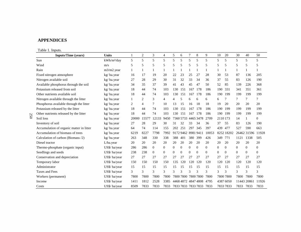
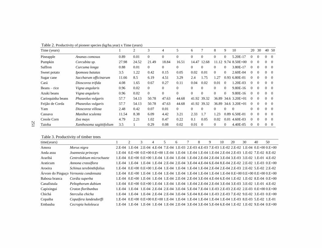
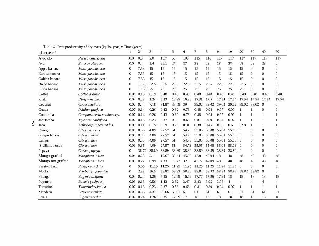
Table 1 shows inputs and outputs. Output is presented in APPENDICES (Tables 2, 3 and 4).

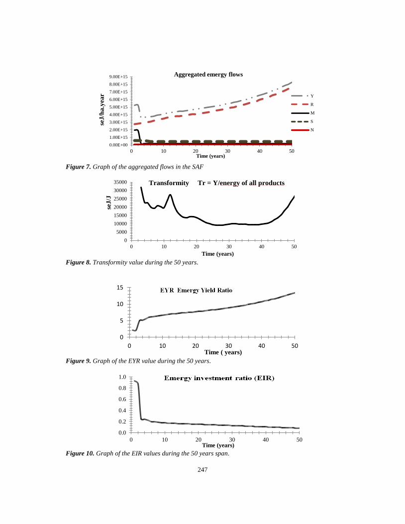
Figure 7 presents the values for the Emergy aggregated flows during the development of the SAF. It

may be observed that the values of renewable resources are higher than the non-renewable ones, once

SAF uses the minimum amount of non-renewable resources.

Hereafter, the emergy indices are presented.

Transformity assesses the quality of the energy flow and it allows comparisons with other

systems: Tr = Y / Ep. For the case studied, transformity decreases and grow until year 15, is constant

through 25 years, and increases after 40 (Figure 8).

The Emergy Yield Ratio is the ratio of emergy invested (Y) to economic investment (F): EYR =

Y/F, in other words: EYR = ((R+N)/F) + 1. It provides a measure of the incorporation of nature’s

resources per unit of economic contribution. In chemical agriculture it varies from 1.05 to 1.35. The

value for agroforestry varied from 1.2 (first year) to 13 (47th year). In the third year it already achieved

5, a very high value. The SAF shows a high emergy yield that increases along the growing period. This

means that the SAF transfers net emergy to the surrounding region, an important fact for public

policies that consider oil supply reduction as well as carbon sequestration (Figure 9).

The Emergy Investment Ratio (EIR) measures society’s investment to produce a given good in

relation to the nature’s contribution. It may be interpreted as an index of competitiveness that shows

the quantity of economic resources (F) that is needed to obtain resources from nature (I): EIR=F/I

(Figure 10). The EIR value for conventional chemical agriculture varies from 5 and 8. In this case. the

lower the better. The estimated value of EIR drops rapidly from 5.65 in the first year to 0.87 in the

second and keeps falling until it reaches 0.08 in 48th year. The SAF demands a substantial initial

investment to provide self-sufficiency and independence from industrial economic resources.

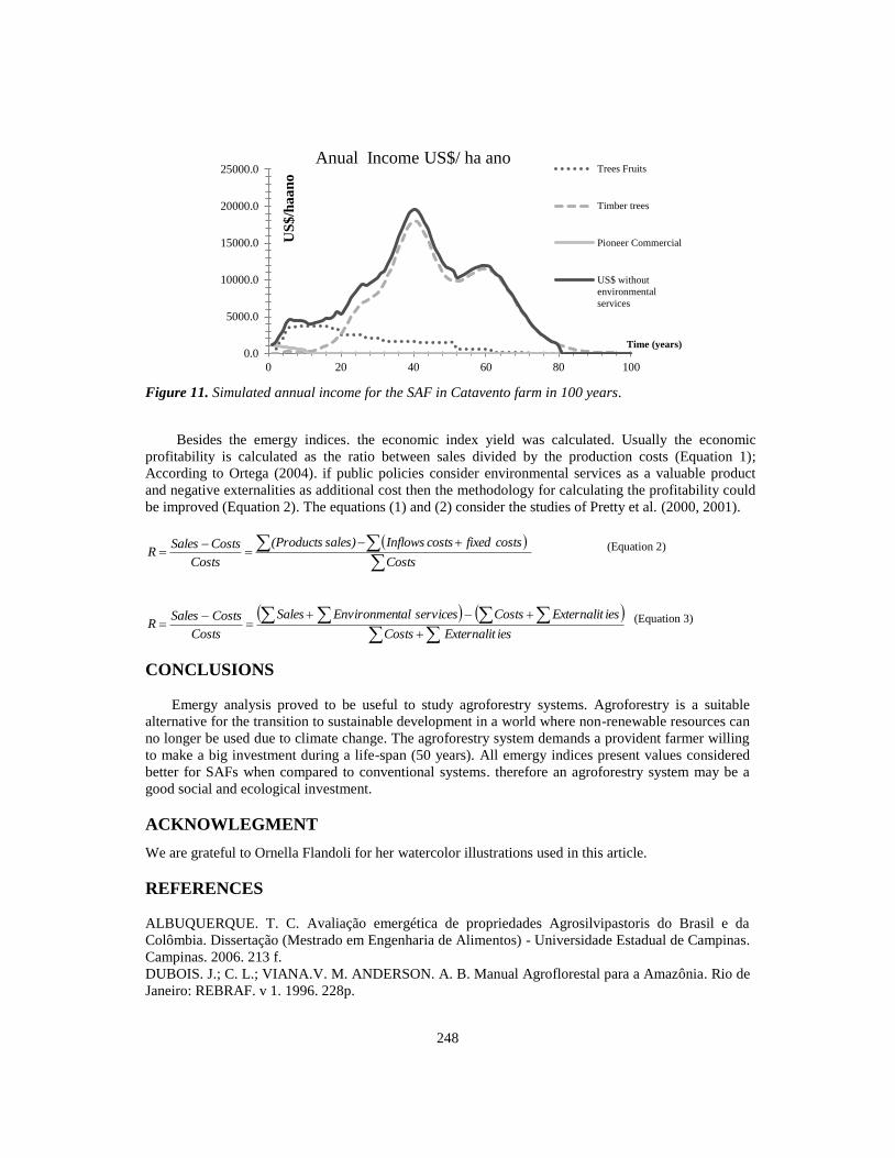
Income curves were obtained considering sales and costs of SAF along time. (Figure 11). The

production cost is high during the first three years. when investment is made. From the economic point

of view. the SAF showed to provide a mean income of US$ 654/month for the patronal system and

US$ 849/month for the family managed farm. a much better values than the conventional agriculture

systems but the SAF farmer should be prepared for an initial stage of low income that can take several

years.

The cost is high only during the first three years. because this is the period of implementation of

the system (when fixed investment is made).

246

Figure 6. Biomass for all species in the SAF area in Catavento farm.

Table 1. Emergy Flows, Outputs, Emergy Indices, Economics and Social.

Emergy

Flows Expression Description 10 years 20 years 30 years 40 years 50 years

I Natural Contribution R+N 3,50E+15 4,09E+15 4.82E+15 5.93E+15 7.62E+15

R Renewable Resources R 3.50E+15 4.09E+15 4.82E+15 5.93E+15 7.62E+15

N Non Renewable

Resources N 4.00E+07 1.90E+06 1.06E+05 6.95E+03 5.06E+02

F Feedback from Economy M+S 6.10E+14 6.11E+14 6.11E+14 6.11E+14 6.11E+14

M Materials M 1.60E+14 1.56E+14 1.56E+14 1.56E+14 1.56E+14

S Services S 4.60E+14 4.55E+14 4.55E+14 4.55E+14 4.55E+14

Y Total Emergy: I+F 4.10E+15 4.70E+15 5.43E+15 6.54E+15 8.23E+15

Outputs Expression Description 10 years 20 years 30 years 40years 50 years

Ep Energy of Products Ep 3.20E+09 2.13E+09 2.31E+09 2.16E+09 1.93E+09

Internal Stocks Stk 2.00E+11 4.23E+11 6.43E+11 6.99E+11 2.84E+11

Es Internal Stocks Changes ΔStk 1.20E+17 1.80E+17 2.73E+17 4.12E+17 6.13E+17

E Total Energy Ep+Es 2.10E+11 4.25E+11 6.45E+11 7.02E+11 2.86E+11

Emergy

Indices Expression Description 10 years 20 years 30 years 40years 50 years

Tr Solar Transformity Y/E 2.00E+04 1.11E+04 8.41E+03 9.32E+03 2.88E+04

EYR Emergy Yield Ratio Y/F 6.70E+00 7.69E+00 8.88E+00 1.07E+01 1.35E+01

EIR Emergy Investment Ratio F/I 1.70E-01 1.50E-01 1.27E-01 1.03E-01 8.02E-02

%R Renewability R/Y*100 8.50E+01 8.70E+01 8.87E+01 9.07E+01 9.26E+01

EER Emergy Exchange Ratio Y/In*emdollar 2.50E-01 2.06E-01 1.26E-01 8.44E-02 1.86E-01

Economics

and Social Expression Description 10 years 20 years 30 years 40years 50 years

In Income 4.50E+03 6.16E+03 1.17E+04 2.09E+04 1.19E+04

C Costs 7.80E+03 7.83E+03 7.83E+03 7.83E+03 7.83E+03

P Profits In-C -3.40E+03 -1.67E+03 3.82E+03 1.31E+04 4.10E+03

Y Yield P/C -4.30E-01 -2.13E-01 4.88E-01 1.67E+00 5.24E-01

Employees workers/ha 1.00E+00 1.00E+00 1.00E+00 1.00E+00 1.00E+00

0.00

5,000.00

10,000.00

15,000.00

20,000.00

25,000.00

30,000.00

0 10 20 30 40 50

kg

of

dry

bio

ma

ss/h

a.y

ea

r

Time (years)

Biomass production of the four types of plants introduced

in the SAF Fruit tree

Wood

Comercial

Non

Comercial

247

Figure 7. Graph of the aggregated flows in the SAF

Figure 8. Transformity value during the 50 years.

Figure 9. Graph of the EYR value during the 50 years.

Figure 10. Graph of the EIR values during the 50 years span.

0.00E+00

1.00E+15

2.00E+15

3.00E+15

4.00E+15

5.00E+15

6.00E+15

7.00E+15

8.00E+15

9.00E+15

0 10 20 30 40 50

seJ

/ha

.yea

r

Time (years)

Aggregated emergy flows

Y

R

M

S

N

0

5000

10000

15000

20000

25000

30000

35000

0 10 20 30 40 50

seJ

/J

Time (years)

Transformity Tr = Y/energy of all products

0

5

10

15

0 10 20 30 40 50Time ( years)

0.0

0.2

0.4

0.6

0.8

1.0

0 10 20 30 40 50Time (years)

248

Figure 11. Simulated annual income for the SAF in Catavento farm in 100 years.

Besides the emergy indices. the economic index yield was calculated. Usually the economic

profitability is calculated as the ratio between sales divided by the production costs (Equation 1);

According to Ortega (2004). if public policies consider environmental services as a valuable product

and negative externalities as additional cost then the methodology for calculating the profitability could

be improved (Equation 2). The equations (1) and (2) consider the studies of Pretty et al. (2000, 2001).

Costs

costs fixedcostsInflowssales)(Products

Costs

CostsSalesR (Equation 2)

iesExternalitCosts

iesExternalitCosts servicestalEnvironmenSales

Costs

CostsSalesR

(Equation 3)

CONCLUSIONS

Emergy analysis proved to be useful to study agroforestry systems. Agroforestry is a suitable

alternative for the transition to sustainable development in a world where non-renewable resources can

no longer be used due to climate change. The agroforestry system demands a provident farmer willing

to make a big investment during a life-span (50 years). All emergy indices present values considered

better for SAFs when compared to conventional systems. therefore an agroforestry system may be a

good social and ecological investment.

ACKNOWLEGMENT

We are grateful to Ornella Flandoli for her watercolor illustrations used in this article.

REFERENCES

ALBUQUERQUE. T. C. Avaliação emergética de propriedades Agrosilvipastoris do Brasil e da

Colômbia. Dissertação (Mestrado em Engenharia de Alimentos) - Universidade Estadual de Campinas.

Campinas. 2006. 213 f.

DUBOIS. J.; C. L.; VIANA.V. M. ANDERSON. A. B. Manual Agroflorestal para a Amazônia. Rio de

Janeiro: REBRAF. v 1. 1996. 228p.

0.0

5000.0

10000.0

15000.0

20000.0

25000.0

0 20 40 60 80 100

US

$/h

aa

no

Time (years)

Anual Income US$/ ha ano Trees Fruits

Timber trees

Pioneer Commercial

US$ without

environmental

services

249

CAIRNS. M.A.. BROWN. S.. HELMER. E.H.. BAUMGARDNER. G.A. Root biomass allocation in

the world’s upland forests. O ecologica. 1997. 111: 1–11.

COOPERAFLORESTA: Associação dos Agricultores Agroflorestais de Barra do Turvo/ SP: Site:

http://cooperafloresta.org.br/

COSTA. R. C. Pagamentos por serviços ambientais: limites e oportunidades para o desenvolvimento

sustentável da agricultura Família na Amazônia Brasileira. Dissertação (Doutorado em Ciência

Ambiental). Universidade de São Paulo. 2008 246f.

GÖTSCH. E. (1995). O Renascer da Agricultura. Rio de Janeiro: AS-PTA. 1995. 22p.

INSTITUTE OF AGRICULTURAL ECONOMICS. IEA. 2012. Consulta no dia 16 de março de 2012

http://www.iea.sp.gov.br/out/verTexto.php?codTexto=741

LUNDGREN. B. ICRAF’S; The first ten years. Agroforestry systems (5). p.97-217. 1987.

MARGULIS. Sergio. 2003 Causas do Desmatamento da Amazônia Brasileira - 1ª edição - Brasília –

2003 100p.ISBN: 85-88192-10-1

MANUAL AGROFLORESTAL. Peter Herman May Cassio. Murilo Moreira Trovatto Organizadores

Guilherme dos Santos Floriani Jean Clement Laurent Dubois Jorge Luiz Vivan. Brasília.2 de outubro

de 2008.

ODUM. H.T.. M.T. BROWN. AND S. L. BRANDT-WILLIAMS. 2000. Folio #1: Introduction and

global budget. Handbook of Emergy Evaluation: A compendium of data for emergy computation

issued in a series of folios. Center for Environmental Policy. Univ. of Florida. Gainesville.

ODUM. H.T. Environmental Accounting: emergy and decision making. John Wiley. NY. 1996. 370

pp.

OLIVEIRA. E. B.; SCHREINER. H. G. Caracterização e análise estatística de experimentos de

agrossilvicultura. Boletim de Pesquisa Florestal. Curitiba. v. 15. p. 19-40. 1987.

ODUM. H.T. 2000. Folio #2: Emergy of global Processes. Handbook of Emergy Evaluation: A

compendium of data for emergy computation issued in a series of folios Center for Environmental

Policy. Univ. of Florida. Gainesville.

ODUM. H.T. 1996. Environmental Accounting: Emergy and Environmental Decision Making John

Wiley and Sons. New York.

ORTEGA E. DINIZ. M.H ANAMI G. 2002. 3rd

Biennal International Workshop Advances in Energy

Studies. Reconsidering the importance of Energy. Porto Venere. Italy September 24/28 2002.

Editoriali Padova.

PENEIREIRO. F. M. et al. Apostila do educador agroflorestal. Introdução aos sistemas agroflorestais –

um guia técnico. Arboreto. UFAC. Rio Branco. 2008. 77p.

PRETTY. J.N. et al.; An assessment of the total external costs of UK agriculture. Agricultural

Systems. 2000.

PRETTY. J.N. et al.; Policy and Practice: Policy Challenges and Priorities for Internalizing the

Externalities of Modern Agriculture. Journal of Environmental Planning and Management. v.44 (2). p.

263-283. 2001.

RONCON. T. J.. 2009. Evolução dos serviços ambientais durante a recuperação uma floresta nativa

em área de preservação permanente. 2009-2010. Universidade Federal de São Carlos.

RONCON. Thiago Junqueira; BESKOW. Paulo Roberto; ORTEGA. Enrique; MARGARIDO. Luiz

Antonio Corrêa; DINIZ JUNIOR. Guaraci M. Valoração ecológica aplicada a áreas de preservação

permanente. Rev. Bras.de Agroecologia. 7(3): 3-15 (2012).

VIVAN. J. L. Agricultura & Floresta – Princípios de uma Interação Vital. AS-PTA/Editora

Agropecuária. 1998. 207p.

25

0

APPENDICES

Table 1. Inputs.

Inputs/Time (years) Units 1 2 3 4 5 6 7 8 9 10 20 30 40 50

Sun kWh/m²/day 5 5 5 5 5 5 5 5 5 5 5 5 5 5

Wind m/s 5 5 5 5 5 5 5 5 5 5 5 5 5 5

Rain m3/m2.year 1 1 1 1 1 1 1 1 1 1 1 1 1 1

Fixed nitrogen atmosphere kg/ ha.year 16 17 19 20 22 23 25 27 28 30 53 87 136 205

Nitrogen available soil kg/ ha.year 27 28 29 30 31 32 33 34 36 37 55 83 126 190

Available phosphorus through the soil kg/ ha.year 34 35 37 39 41 43 45 47 50 52 85 139 226 368

Potassium released from soil kg/ ha.year 18 44 74 103 130 151 167 178 186 190 331 341 351 361

Other nutrients available soil kg/ ha.year 18 44 74 103 130 151 167 178 186 190 199 199 199 199

Nitrogen available through the litter kg/ ha.year 1 2 3 4 4 5 6 6 6 6 7 7 7 7

Phosphorus available through the litter kg/ ha.year 2 4 7 10 13 15 16 18 18 19 20 20 20 20

Potassium released by the litter kg/ ha.year 18 44 74 103 130 151 167 178 186 190 199 199 199 199

Other nutrients released by the litter kg/ ha.year 18 44 74 103 130 151 167 178 186 190 199 199 199 199

Soil loss kg/ ha.year 20000 15577 12133 9450 7360 5733 4465 3478 2709 2110 173 14 1 0

Inventory of soil kg/ ha.year 27 28 29 30 31 32 33 34 36 37 55 83 126 190

Accumulation of organic matter in litter kg/ ha.year 64 74 114 155 202 251 297 345 397 439 477 527 590 663

Accumulation of biomass of trees kg/ ha.year 6219 8227 7798 7992 9172 9462 8981 9411 10053 8252 18202 26462 31596 11928

Calculation of carbon (Biomass /2) kg/ ha.year 263 348 330 338 388 401 380 399 426 349 771 1121 1338 505

Diesel tractor L/ha.year 20 20 20 20 20 20 20 20 20 20 20 20 20 20

Thermo-phosphate (organic input) US$/ ha/year 286 286 0 0 0 0 0 0 0 0 0 0 0 0

Seedlings and seeds US$/ ha/year 238 238 0 0 0 0 0 0 0 0 0 0 0 0

Conservation and depreciation US$/ ha/year 27 27 27 27 27 27 27 27 27 27 27 27 27 27

Temporary labor US$/ ha/year 150 150 150 150 135 120 120 120 120 120 120 120 120 120

Administrator US$/ ha/year 15 15 15 15 15 15 15 15 15 15 15 15 15 15

Taxes and Fees US$/ ha/year 3 3 3 3 3 3 3 3 3 3 3 3 3 3

Workers (permanent) US$/ ha/year 7800 7800 7800 7800 7800 7800 7800 7800 7800 7800 7800 7800 7800 7800

Income US$/ ha/year 1411 1812 2528 3385 4468 4872 4847 4808 4795 4387 6050 11443 20861 11926

Costs US$/ ha/year 8509 7833 7833 7833 7833 7833 7833 7833 7833 7833 7833 7833 7833 7833

25

1

Table 2. Productivity of pioneer species (kg/ha.year) x Time (years)

Time (years) 1 2 3 4 5 6 7 8 9 10 20 30 40 50

Pineapple Ananas comosus 0.89 0.01 0 0 0 0 0 0 0 5.20E-17 0 0 0 0

Pumpkin Corcubita sp. 27.98 24.52 21.49 18.84 16.51 14.47 12.68 11.12 9.74 8.50E+00 0 0 0 0

Saffron Curcuma longa 0.88 0.01 0 0 0 0 0 0 0 3.80E-17 0 0 0 0

Sweet potato Ipomoea batatas 3.5 1.22 0.42 0.15 0.05 0.02 0.01 0 0 2.60E-04 0 0 0 0

Sugar cane Saccharum officinarum 11.66 8.5 6.19 4.51 3.29 2.4 1.75 1.27 0.93 6.80E-01 0 0 0 0

Cará Dioscorea trifida 4.08 1.65 0.67 0.27 0.11 0.04 0.02 0.01 0 1.20E-03 0 0 0 0

Beans – rice Vigna angularis 0.96 0.02 0 0 0 0 0 0 0 9.80E-16 0 0 0 0

Azuki beans Vigna angularis 0.96 0.02 0 0 0 0 0 0 0 9.80E-16 0 0 0 0

Carioquinha beans Phaseolus vulgaris 57.7 54.13 50.78 47.63 44.68 41.92 39.32 36.89 34.6 3.20E+01 0 0 0 0

Feijão de Corda Phaseolus vulgaris 57.7 54.13 50.78 47.63 44.68 41.92 39.32 36.89 34.6 3.20E+01 0 0 0 0

Yam Dioscorea villosa 2.48 0.42 0.07 0.01 0 0 0 0 0 0 0 0 0 0

Cassava Manihot sculenta 11.54 8.38 6.09 4.42 3.21 2.33 1.7 1.23 0.89 6.50E-01 0 0 0 0

Creole Corn Zea mays 4.79 2.21 1.02 0.47 0.22 0.1 0.05 0.02 0.01 4.60E-03 0 0 0 0

Taioba Xanthosoma sagittifolium 3.5 1 0.29 0.08 0.02 0.01 0 0 0 4.40E-05 0 0 0 0

Table 3. Productivity of timber trees

time(years) 1 2 3 4 5 6 7 8 9 10 20 30 40 50

Amora Morus nigra 2.E-04 1.E-04 2.E-04 4.E-04 7.E-04 1.E-03 2.E-03 4.E-03 7.E-03 1.E-02 2.E-02 1.E-04 0.E+00 0.E+00

Anda assu Joannesia princeps 1.E-04 0.E+00 0.E+00 0.E+00 1.E-04 1.E-04 1.E-04 1.E-04 1.E-04 2.E-04 2.E-03 1.E-02 7.E-02 8.E-02

Araribá Centrolobium microchaete 1.E-04 0.E+00 0.E+00 1.E-04 1.E-04 1.E-04 1.E-04 2.E-04 2.E-04 3.E-04 3.E-03 3.E-02 1.E-01 4.E-02

Araticum Annona crassiflora 1.E-04 1.E-04 1.E-04 1.E-04 2.E-04 2.E-04 3.E-04 4.E-04 6.E-04 8.E-04 2.E-02 2.E-02 1.E-03 0.E+00

Aroeira Schinus terebinthifolius 1.E-04 0.E+00 0.E+00 1.E-04 1.E-04 1.E-04 1.E-04 1.E-04 2.E-04 2.E-04 2.E-03 2.E-02 5.E-02 2.E-02

Árvore do Pinguço Vernonia condensata 1.E-04 0.E+00 1.E-04 1.E-04 1.E-04 1.E-04 1.E-04 1.E-04 1.E-04 1.E-04 0.E+00 0.E+00 0.E+00 0.E+00

Babosa branca Cordia superba 1.E-04 0.E+00 1.E-04 1.E-04 1.E-04 2.E-04 2.E-04 3.E-04 4.E-04 6.E-04 1.E-02 1.E-02 8.E-04 0.E+00

Canafistula Peltophorum dubium 1.E-04 0.E+00 0.E+00 1.E-04 1.E-04 1.E-04 1.E-04 2.E-04 2.E-04 3.E-04 3.E-03 3.E-02 1.E-01 4.E-02

Capixingui Croton floribunbus 1.E-04 1.E-04 1.E-04 2.E-04 2.E-04 3.E-04 5.E-04 7.E-04 1.E-03 2.E-03 2.E-02 2.E-03 0.E+00 0.E+00

Chichá Sterculia chicha 1.E-04 1.E-04 1.E-04 2.E-04 2.E-04 3.E-04 5.E-04 8.E-04 1.E-03 2.E-03 7.E-02 9.E-02 3.E-03 0.E+00

Copaiba Copaifera landesdorffi 1.E-04 0.E+00 0.E+00 0.E+00 1.E-04 1.E-04 1.E-04 1.E-04 1.E-04 1.E-04 1.E-03 8.E-03 5.E-02 1.E-01

Embauba Cecropia hololeuca 1.E-04 1.E-04 1.E-04 1.E-04 1.E-04 2.E-04 3.E-04 3.E-04 5.E-04 6.E-04 1.E-02 1.E-02 9.E-04 0.E+00

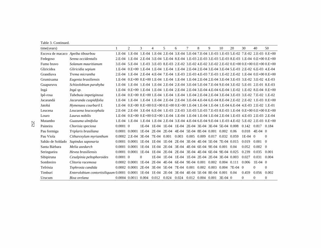
25

2

Table 3. Continued.

time(years) 1 2 3 4 5 6 7 8 9 10 20 30 40 50

Escova de macaco Apeiba tibourbou 1.E-04 1.E-04 1.E-04 1.E-04 2.E-04 3.E-04 5.E-04 7.E-04 1.E-03 1.E-03 5.E-02 7.E-02 2.E-03 0.E+00

Fedegoso Senna occidentalis 2.E-04 1.E-04 2.E-04 3.E-04 5.E-04 8.E-04 1.E-03 2.E-03 3.E-03 5.E-03 8.E-03 1.E-04 0.E+00 0.E+00

Fumo bravo Solanum mauritianum 3.E-04 5.E-04 1.E-03 3.E-03 8.E-03 2.E-02 3.E-02 4.E-02 3.E-02 2.E-02 0.E+00 0.E+00 0.E+00 0.E+00

Gliricidea Gliricidia sepium 1.E-04 0.E+00 1.E-04 1.E-04 1.E-04 1.E-04 2.E-04 2.E-04 3.E-04 3.E-04 5.E-03 2.E-02 6.E-03 4.E-04

Grandiuva Trema micrantha 2.E-04 1.E-04 2.E-04 4.E-04 7.E-04 1.E-03 2.E-03 4.E-03 7.E-03 1.E-02 2.E-02 1.E-04 0.E+00 0.E+00

Grumixama Eugenia brasiliensis 1.E-04 0.E+00 0.E+00 1.E-04 1.E-04 1.E-04 1.E-04 2.E-04 2.E-04 3.E-04 3.E-03 3.E-02 3.E-02 4.E-03

Guapuruvu Schizolobium parahyba 1.E-04 1.E-04 1.E-04 1.E-04 2.E-04 2.E-04 3.E-04 5.E-04 7.E-04 9.E-04 3.E-02 5.E-01 2.E-01 8.E-03

Ingá Ingá sp. 1.E-04 0.E+00 1.E-04 1.E-04 1.E-04 2.E-04 2.E-04 3.E-04 4.E-04 6.E-04 1.E-02 1.E-02 8.E-04 0.E+00

Ipê-rosa Tabebuia impetiginosa 1.E-04 0.E+00 0.E+00 1.E-04 1.E-04 1.E-04 1.E-04 2.E-04 2.E-04 3.E-04 3.E-03 3.E-02 7.E-02 1.E-02

Jacarandá Jacaranda cuspidifolia 1.E-04 1.E-04 1.E-04 1.E-04 2.E-04 2.E-04 3.E-04 4.E-04 6.E-04 8.E-04 2.E-02 2.E-02 1.E-03 0.E+00

Jatobá Hymenaea courbaril L 1.E-04 0.E+00 0.E+00 0.E+00 0.E+00 0.E+00 1.E-04 1.E-04 1.E-04 1.E-04 6.E-04 4.E-03 2.E-02 1.E-01

Leucena Leucaena leucocephala 2.E-04 2.E-04 3.E-04 6.E-04 1.E-03 2.E-03 3.E-03 5.E-03 7.E-03 8.E-03 1.E-04 0.E+00 0.E+00 0.E+00

Louro Laurus nobilis 1.E-04 0.E+00 0.E+00 0.E+00 1.E-04 1.E-04 1.E-04 1.E-04 1.E-04 2.E-04 1.E-03 4.E-03 2.E-03 2.E-04

Mutambo Guazuma ulmifolia 1.E-04 1.E-04 1.E-04 1.E-04 2.E-04 3.E-04 4.E-04 6.E-04 9.E-04 1.E-03 4.E-02 5.E-02 2.E-03 0.E+00

Paineira Chorisia speciosa 0.0001 0 1E-04 1E-04 1E-04 1E-04 2E-04 3E-04 3E-04 5E-04 0.008 0.142 0.817 0.184

Pau formiga Triplaris brasiliana 0.0001 0.0001 1E-04 2E-04 2E-04 4E-04 5E-04 8E-04 0.001 0.002 0.06 0.018 4E-04 0

Pau Viola Citharexylum myrianthum 0.0002 2.E-04 3E-04 7E-04 0.001 0.003 0.005 0.009 0.017 0.032 0.059 1E-04 0 0

Sabão de Soldado Sapindus saponaria 0.0001 0.0001 1E-04 1E-04 1E-04 2E-04 3E-04 4E-04 5E-04 7E-04 0.015 0.019 0.001 0

Santa Bárbara Melia azedarch 0.0001 0.0001 1E-04 1E-04 2E-04 3E-04 4E-04 6E-04 9E-04 0.001 0.04 0.052 0.002 0

Seringueira Hevea brasiliensis 0.0001 0.0001 1E-04 1E-04 2E-04 2E-04 3E-04 4E-04 6E-04 9E-04 0.025 0.239 0.035 0.001

Sibipiruna Cesalpinia peltophoroides 0.0001 0 0 1E-04 1E-04 1E-04 1E-04 2E-04 2E-04 3E-04 0.003 0.027 0.031 0.004

Sombreiro Clitoria racemosa 0.0002 0.0001 1E-04 2E-04 4E-04 6E-04 9E-04 0.001 0.002 0.004 0.111 0.006 1E-04 0

Tefrósia Tephrosia candida 0.0002 0.0001 2E-04 3E-04 5E-04 7E-04 0.001 0.002 0.003 0.004 7E-04 0 0 0

Timburí Enterolobium contortisiliquum 0.0001 0.0001 1E-04 1E-04 2E-04 3E-04 4E-04 5E-04 8E-04 0.001 0.04 0.459 0.056 0.002

Urucum Bixa orelana 0.0004 0.0011 0.004 0.012 0.024 0.024 0.012 0.004 0.001 3E-04 0 0 0 0

25

3

Table 4. Fruit productivity of dry mass (kg/ ha year) x Time (years)

time(years) 1 2 3 4 5 6 7 8 9 10 20 30 40 50

Avocado Persea americana 0.0 0.3 2.0 13.7 58 103 115 116 117 117 117 117 117 117

Açai Euterpe oleracea 0.0 0.4 5.4 22.1 27 27 28 28 28 28 28 28 28 0

Apple banana Musa paradisiaca 0 7.53 15 15 15 15 15 15 15 15 15 0 0 0

Nanica banana Musa paradisiaca 0 7.53 15 15 15 15 15 15 15 15 15 0 0 0

Golden banana Musa paradisiaca 0 7.53 15 15 15 15 15 15 15 15 15 0 0 0

Bread banana Musa paradisiaca 0 11.28 22.5 22.5 22.5 22.5 22.5 22.5 22.5 22.5 22.5 0 0 0

Silver banana Musa paradisiaca 0 12.53 25 25 25 25 25 25 25 25 25 0 0 0

Coffee Coffea arabica 0.08 0.13 0.19 0.48 0.48 0.48 0.48 0.48 0.48 0.48 0.48 0.48 0.48 0.48

khaki Diospyros kaki 0.04 0.23 1.24 5.23 12.35 16.32 17.31 17.5 17.54 17.54 17.54 17.54 17.54 17.54

Coconut Cocos nucifera 0.02 0.44 7.18 31.87 38.59 39 39.02 39.02 39.02 39.02 39.02 39.02 0 0

Guava Psidium guajava 0.07 0.14 0.26 0.43 0.62 0.78 0.88 0.94 0.97 0.99 1 1 0 0

Guabiroba Campomanesia xanthocarpa 0.07 0.14 0.26 0.43 0.62 0.78 0.88 0.94 0.97 0.99 1 1 1 1

Jabuticaba Myciaria cauliflora 0.07 0.13 0.23 0.37 0.53 0.68 0.81 0.89 0.94 0.97 1 1 1 1

Jaca Arthocarpus heterofilus 0.09 0.11 0.15 0.19 0.25 0.31 0.38 0.45 0.53 0.6 0.98 1 1 1

Orange Citrus sinensis 0.03 0.35 4.09 27.57 51 54.73 55.05 55.08 55.08 55.08 0 0 0 0

Galego lemon Citrus limonia 0.03 0.35 4.09 27.57 51 54.73 55.05 55.08 55.08 55.08 0 0 0 0

Lemon Citrus limon 0.03 0.35 4.09 27.57 51 54.73 55.05 55.08 55.08 55.08 0 0 0 0

Siciliano lemon Citrus limon 0.03 0.35 4.09 27.57 51 54.73 55.05 55.08 55.08 55.08 0 0 0 0

Papaya Carica papaya 0 38.79 38.89 38.89 38.89 38.89 38.89 38.89 38.89 38.89 0 0 0 0

Mango grafted Mangifera indica 0.04 0.28 2.1 12.67 35.44 45.98 47.8 48.04 48 48 48 48 48 48

Mango not grafted Mangifera indica 0.05 0.22 0.99 4.33 15.22 32.9 43.77 47.09 48 48 48 48 48 48

Passion fruit Passiflora edulis 0 5.65 11.25 11.25 11.25 11.25 11.25 11.25 11.25 11.25 0 0 0 0

Medlar Eriobotrya japonica 0 2.33 56.5 58.82 58.82 58.82 58.82 58.82 58.82 58.82 58.82 58.82 0 0

Pitanga Eugenia uniflora 0.04 0.24 1.26 5.35 12.69 16.76 17.77 17.96 17.99 18 18 18 18 18

Pupunha Bactris gasipaes 0.05 0.18 0.56 1.43 2.62 3.47 3.83 3.95 3.98 4 4 4 4 4

Tamarind Tamarindus indica 0.07 0.13 0.23 0.37 0.53 0.68 0.81 0.89 0.94 0.97 1 1 1 1

Mandarin Citrus reticulata 0.03 0.36 4.37 30.66 56.91 61 61 61 61 61 61 61 61 61

Uvaia Eugenia uvalha 0.04 0.24 1.26 5.35 12.69 17 18 18 18 18 18 18 18 18

25

4