EMGT 501

HW #1 SolutionsChapter 2 - SELF TEST 18

Chapter 2 - SELF TEST 20

Chapter 3 - SELF TEST 28

Chapter 4 - SELF TEST 3

Chapter 5 - SELF TEST 6

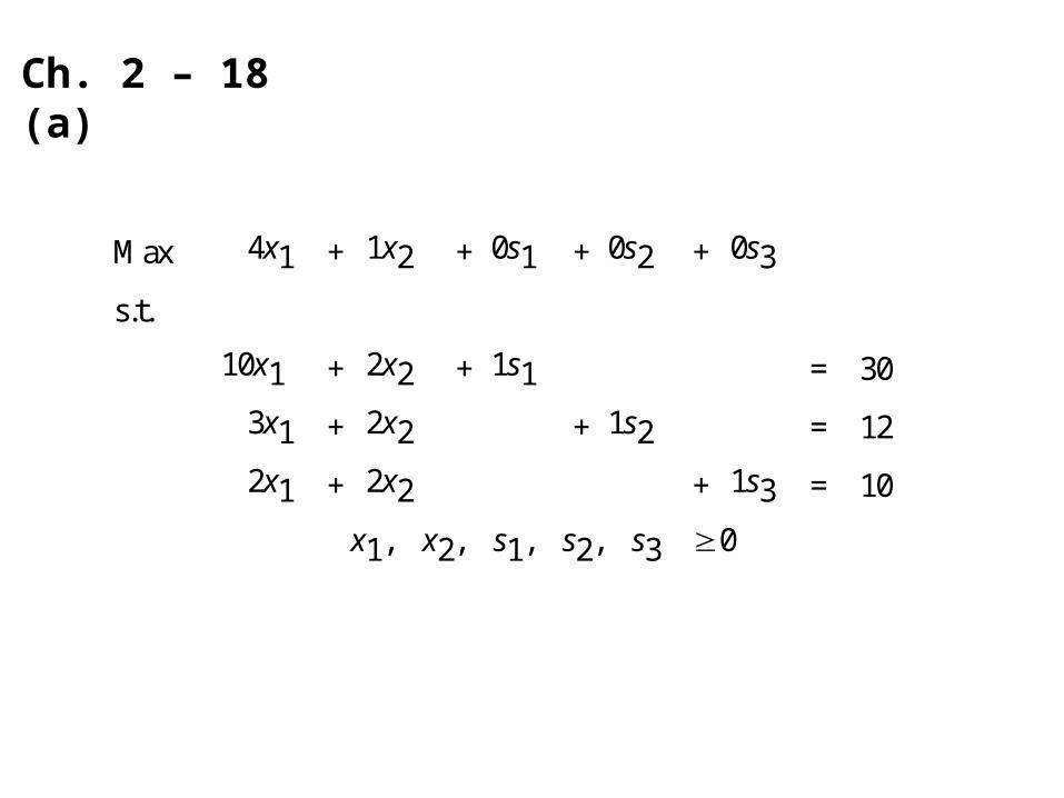
Ch. 2 – 18(a)

Max 4x1 + 1x2 + 0s1 + 0s2 + 0s3

s.t.

10x1 + 2x2 + 1s1 = 30

3x1 + 2x2 + 1s2 = 12

2x1 + 2x2 + 1s3 = 10

x1, x2, s1, s2, s3 0

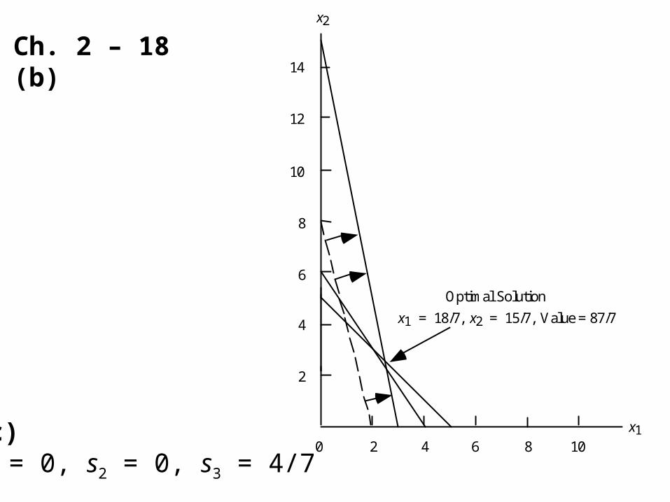
Ch. 2 – 18(b)

x2

x10 2 4 6 8 10

2

4

6

8

10

12

14

Optimal Solution

x1 = 18/7, x2 = 15/7, Value = 87/7

(c)s1 = 0, s2 = 0, s3 = 4/7

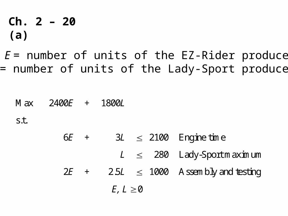
Ch. 2 – 20(a)

Let E = number of units of the EZ-Rider produced L = number of units of the Lady-Sport produced

Max 2400E + 1800L

s.t.

6E + 3L 2100 Engine time

L 280 Lady-Sport maximum

2E + 2.5L 1000 Assembly and testing

E, L 0

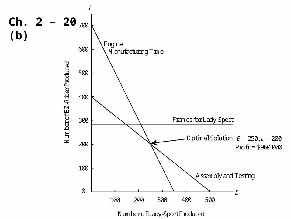
Ch. 2 – 20(b)

0

L

Profit = $960,000

Optimal Solution

100

200

300

400

500

600

700

100 200 300 400 500E

Engine Manufacturing Time

Frames for Lady-Sport

Assembly and Testing

E = 250, L = 200

Number of Lady-Sport Produced

Num

ber

of E

Z-R

ider

Pro

duce

d

Ch. 2 – 20(c)

The binding constraints are the manufacturing time and the assembly and testing time.

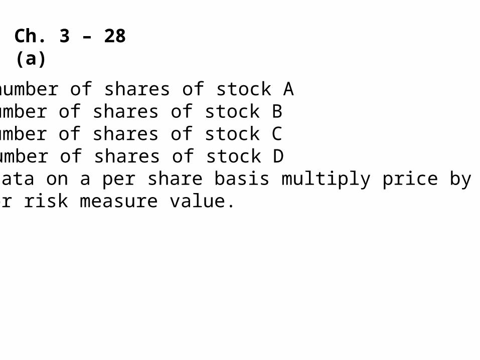
Ch. 3 – 28(a)

Let A = number of shares of stock AB = number of shares of stock BC = number of shares of stock CD = number of shares of stock D

To get data on a per share basis multiply price by rate of return or risk measure value.

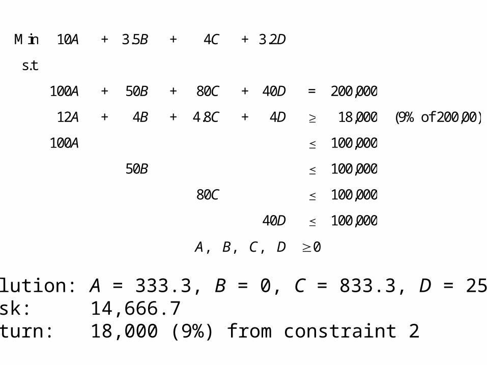
Min 10A + 3.5B + 4C + 3.2D

s.t.

100A + 50B + 80C + 40D = 200,000

12A + 4B + 4.8C + 4D 18,000 (9% of 200,00)

100A 100,000

50B 100,000

80C 100,000

40D 100,000

A, B, C, D 0

Solution: A = 333.3, B = 0, C = 833.3, D = 2500Risk: 14,666.7Return: 18,000 (9%) from constraint 2

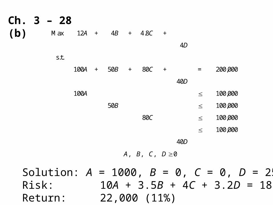
Ch. 3 – 28(b) Max 12A + 4B + 4.8C +

4D

s.t.

100A + 50B + 80C +

40D

= 200,000

100A 100,000

50B 100,000

80C 100,000

40D

100,000

A, B, C, D 0

Solution: A = 1000, B = 0, C = 0, D = 2500Risk: 10A + 3.5B + 4C + 3.2D = 18,000Return: 22,000 (11%)

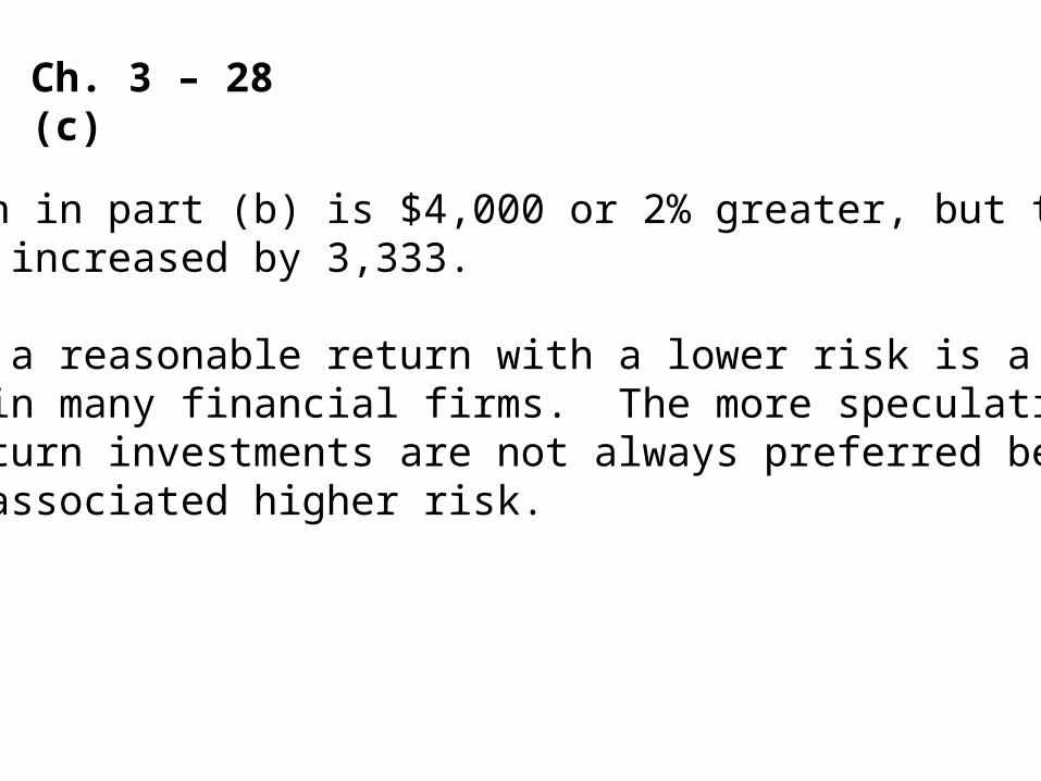
Ch. 3 – 28(c)

The return in part (b) is $4,000 or 2% greater, but the risk index has increased by 3,333.

Obtaining a reasonable return with a lower risk is a preferred strategy in many financial firms. The more speculative, higher return investments are not always preferred because of their associated higher risk.

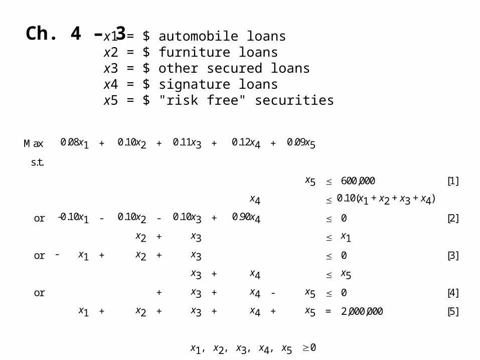
Ch. 4 – 3 x1 = $ automobile loansx2 = $ furniture loansx3 = $ other secured loansx4 = $ signature loansx5 = $ "risk free" securities

Max 0.08x1 + 0.10x2 + 0.11x3 + 0.12x4 + 0.09x5

s.t.

x5 600,000 [1]

x4 0.10(x1 + x2 + x3 + x4)

or -0.10x1 - 0.10x2 - 0.10x3 + 0.90x4 0 [2]

x2 + x3 x1

or - x1 + x2 + x3 0 [3]

x3 + x4 x5

or + x3 + x4 - x5 0 [4]

x1 + x2 + x3 + x4 + x5 = 2,000,000 [5]

x1, x2, x3, x4, x5 0

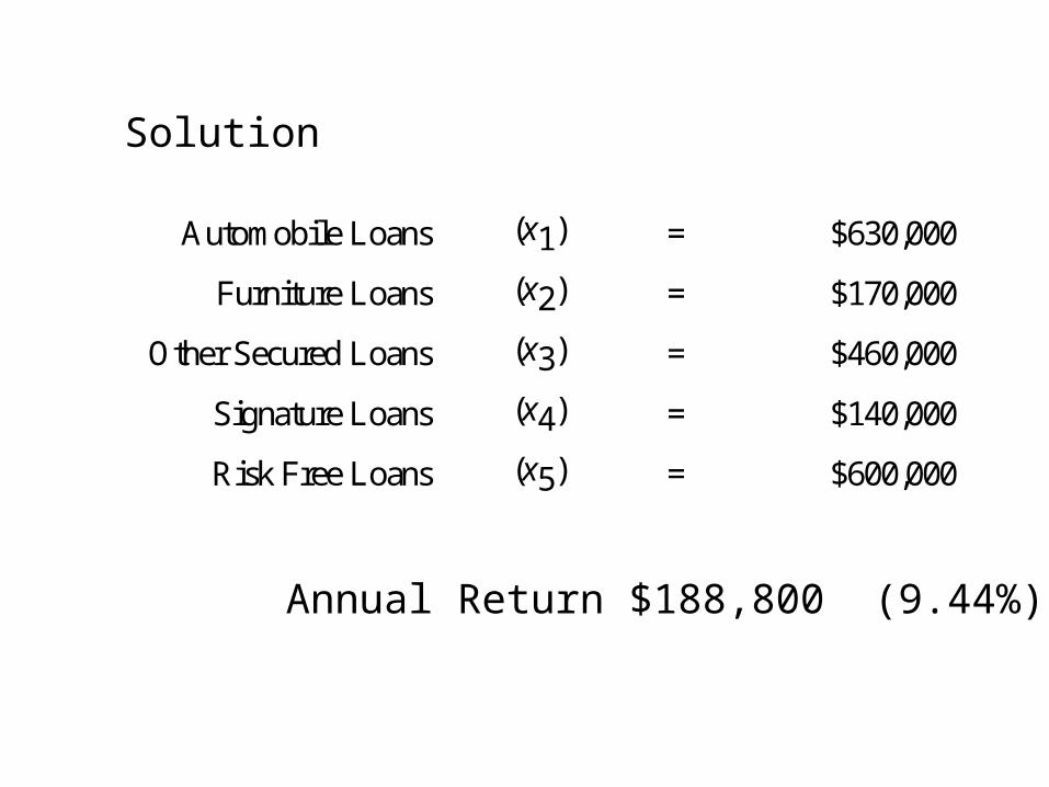
Automobile Loans (x1) = $630,000

Furniture Loans (x2) = $170,000

Other Secured Loans (x3) = $460,000

Signature Loans (x4) = $140,000

Risk Free Loans (x5) = $600,000

Solution

Annual Return $188,800 (9.44%)

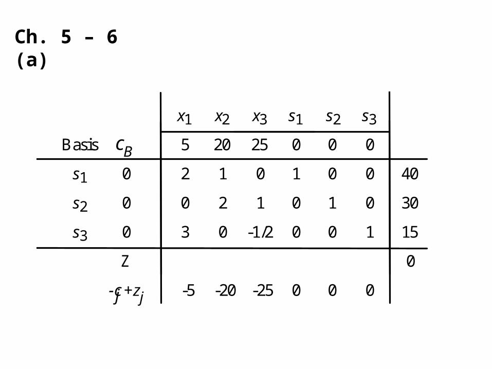
Ch. 5 – 6(a)

x 3

25

0

1

-1/2

-25

s 1

0

1

0

0

0

x 1

5

2

0

3

-5

x 2

1

2

20

0

-20

Basis

s 1

s 2

s 3

c B

0

0

0

Z -c j + z j

s 2

0

0

1

0

0

s 3

0

0

0

1

0

40

30

15

0

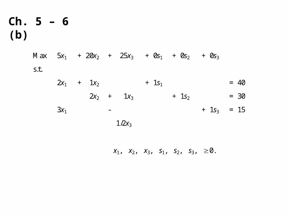
Ch. 5 – 6(b)

Max 5x1 + 20x2 + 25x3 + 0s1 + 0s2 + 0s3

s.t.

2x1 + 1x2 + 1s1 = 40

2x2 + 1x3 + 1s2 = 30

3x1 -

1/2x3

+ 1s3 = 15

x1, x2, x3, s1, s2, s3, 0.

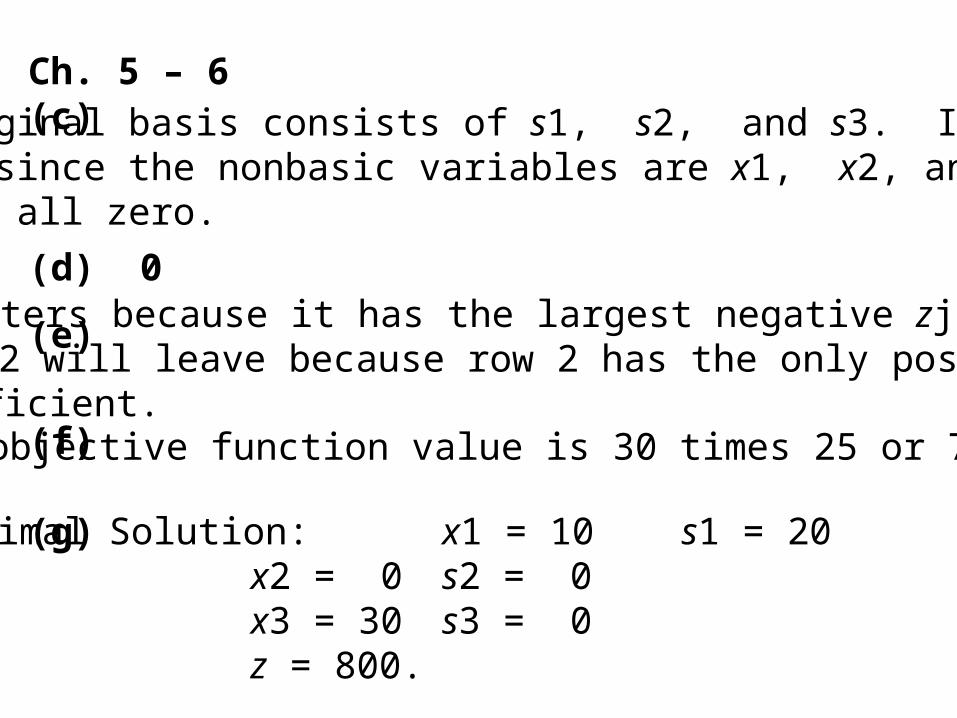
Ch. 5 – 6(c) The original basis consists of s1, s2, and s3. It is the

origin since the nonbasic variables are x1, x2, and x3 and are all zero.

(d) 0

(e)x3 enters because it has the largest negative zj - cj and s2 will leave because row 2 has the only positive coefficient.

(f) 30; objective function value is 30 times 25 or 750.

(g) Optimal Solution: x1 = 10 s1 = 20x2 = 0 s2 = 0x3 = 30 s3 = 0z = 800.

EMGT 501

HW #2Chapter 6 - SELF TEST 21

Chapter 6 - SELF TEST 22

Due Day: Sep 27

s.t.

634Max 321 xxx

20211

3012

1515.01

321

32

321

xxx

xx

xxx

0 , , 321 xxx

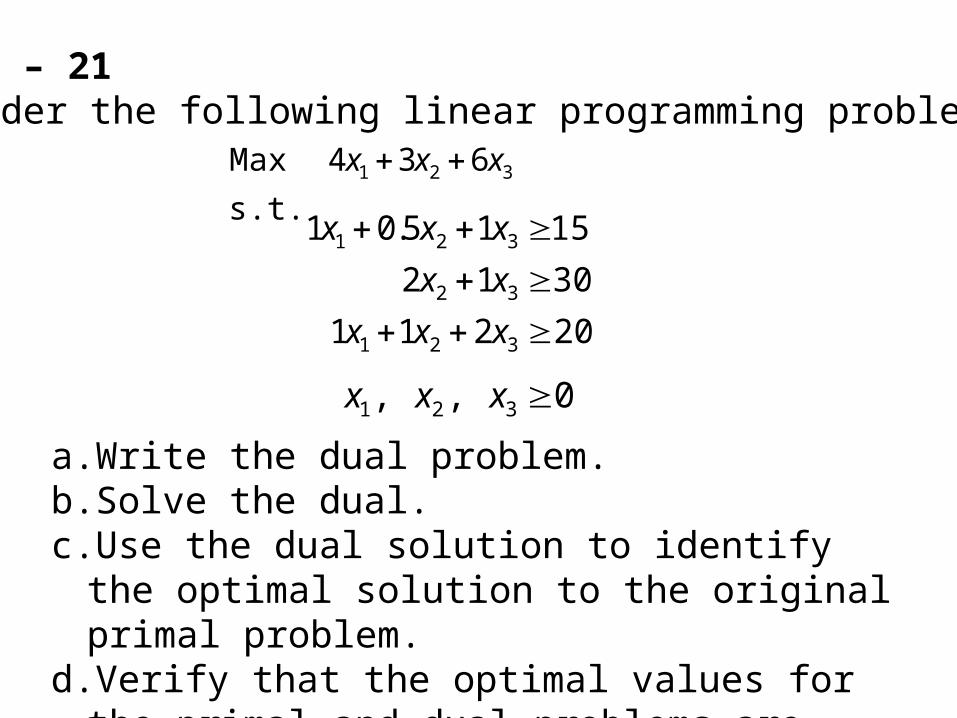
Ch. 6 – 21Consider the following linear programming problem:

a. Write the dual problem.b. Solve the dual.c. Use the dual solution to identify the optimal solution to

the original primal problem.d. Verify that the optimal values for the primal and dual

problems are equal.

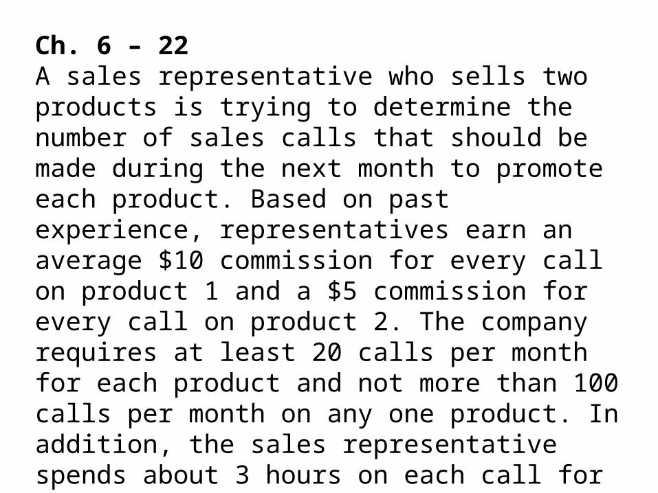
Ch. 6 – 22A sales representative who sells two products is trying to determine the number of sales calls that should be made during the next month to promote each product. Based on past experience, representatives earn an average $10 commission for every call on product 1 and a $5 commission for every call on product 2. The company requires at least 20 calls per month for each product and not more than 100 calls per month on any one product. In addition, the sales representative spends about 3 hours on each call for product 1 and 1 hour on each call for product 2. If 175 selling hours are available next month, how many calls should be made for each of the two products to maximize the commission?

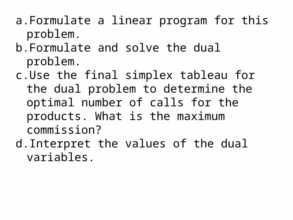
a. Formulate a linear program for this problem.b. Formulate and solve the dual problem.c. Use the final simplex tableau for the dual problem to

determine the optimal number of calls for the products. What is the maximum commission?

d. Interpret the values of the dual variables.

Duality Theory

One of the most important discoveries in the early development of linear programming was the concept of duality.

Every linear programming problem is associated with another linear programming problem called the dual.

The relationships between the dual problem and the original problem (called the primal) prove to be extremely useful in a variety of ways.

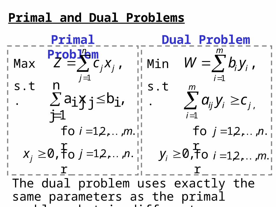
The dual problem uses exactly the same parameters as the primal problem, but in different location.

Primal and Dual Problems

Primal Problem Dual Problem

Max

s.t.

Min

s.t.

n

jjj xcZ

1

,

m

iii ybW

1

,

n

1jijij ,bxa

m

ijiij cya

1,

for for.,,2,1 mi .,,2,1 nj

for .,,2,1 mi for .,,2,1 nj ,0jx ,0iy

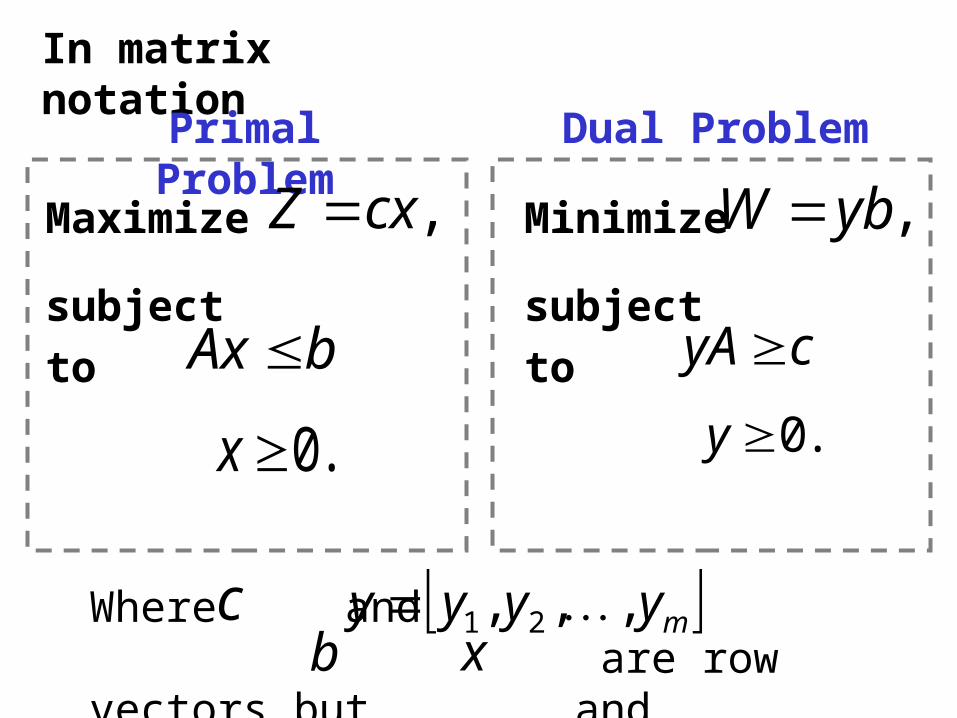
In matrix notation

Primal Problem Dual Problem

Maximize

subject to

.0x .0y

Minimize

subject tobAx cyA

,cxZ ,ybW

Where and are row vectors but and are column vectors.

c myyyy ,,, 21 b x

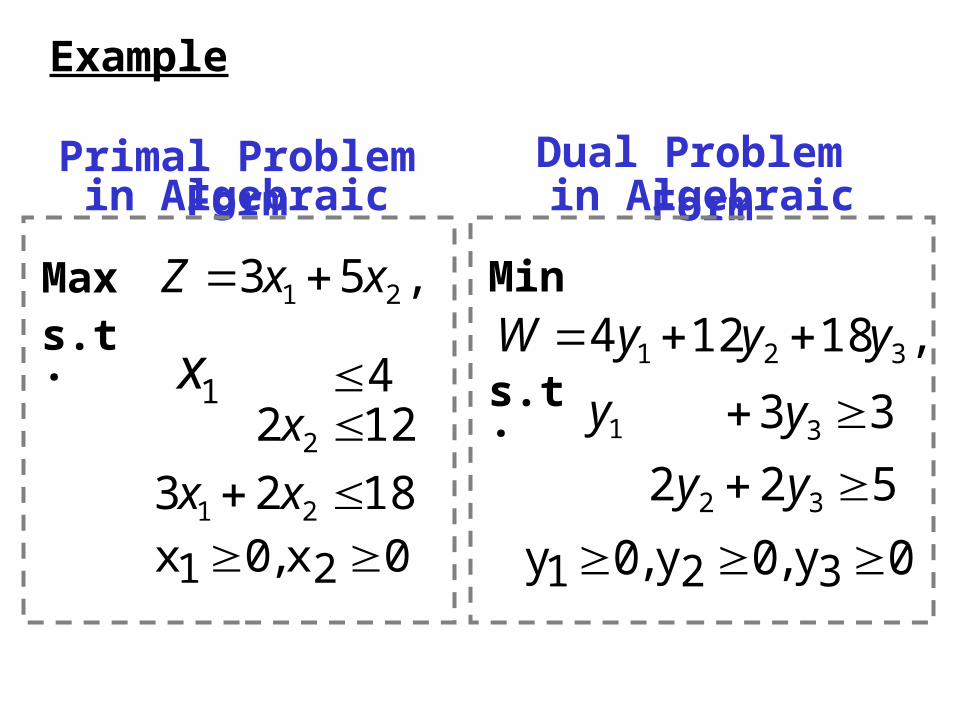
Example

Maxs.t.

Min

s.t.

Primal Problemin Algebraic Form

Dual Problem in Algebraic Form

,53 21 xxZ ,18124 321 yyyW

1823 21 xx

122 2 x41x

0x,0x 21

522 32 yy

33 3 y1y

0y,0y,0y 321

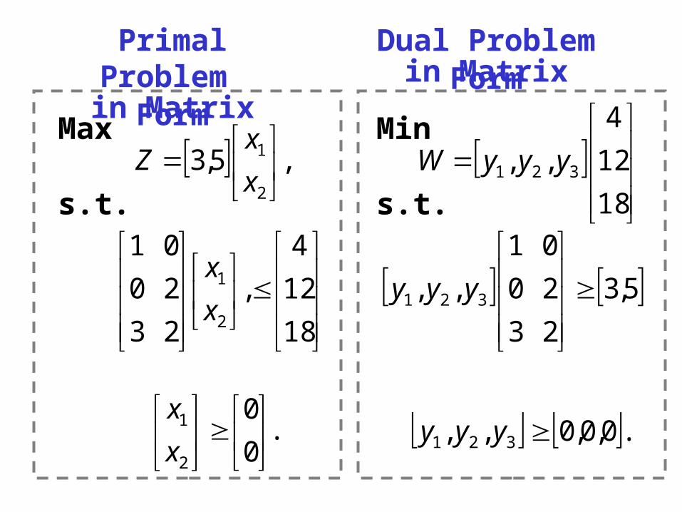
Max

s.t.

Primal Problem in Matrix Form

Dual Problem in Matrix Form

Min

s.t.

,5,32

1

x

xZ

18

12

4

,

2

2

0

3

0

1

2

1

x

x

.0

0

2

1

x

x .0,0,0,, 321 yyy

5,3

2

2

0

3

0

1

,, 321

yyy

18

12

4

,, 321 yyyW

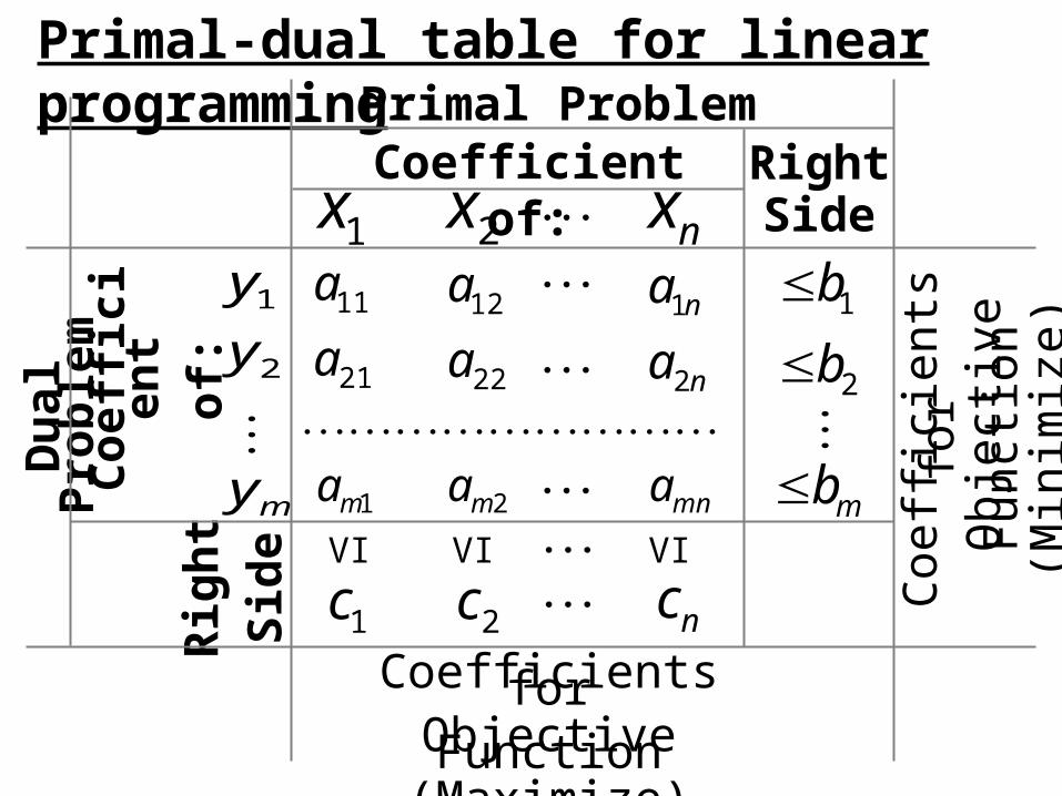
Primal-dual table for linear programmingPrimal Problem

Coefficient of: RightSide

Rig

ht

Sid

eDu

al P

rob

lem

Co

effi

cien

to

f:

my

y

y

2

1

21

11

a

a

22

12

a

a

n

n

a

a

2

1

1x 2x nx

1c 2c ncVI VI VI

Coefficients forObjective Function

(Maximize)

1b

mna2ma1ma

2b

mb

Coe

ffic

ient

s fo

r O

bjec

tive

Fun

ctio

n(M

inim

ize)

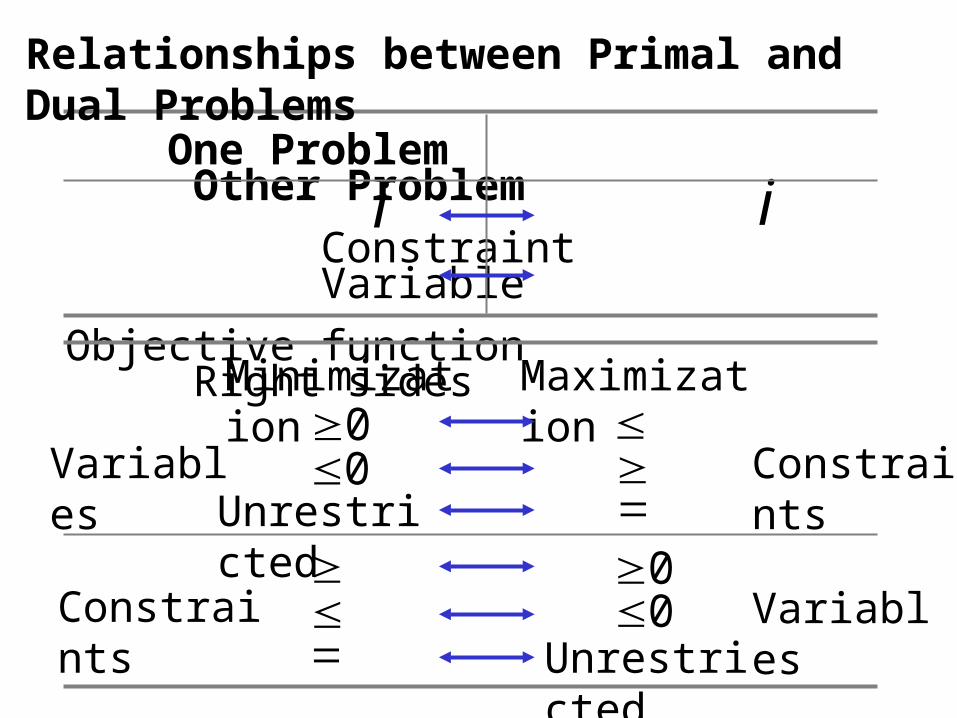
One Problem Other Problem

Constraint Variable

Objective function Right sides

i i

Relationships between Primal and Dual Problems

Minimization Maximization

Variables

Variables

Constraints

Constraints

0

0

0

0

Unrestricted

Unrestricted

The feasible solutions for a dual problem are

those that satisfy the condition of optimality for

its primal problem.

A maximum value of Z in a primal problem

equals the minimum value of W in the dual

problem.

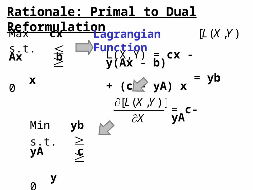
Rationale: Primal to Dual Reformulation

Max cxs.t. Ax b x 0

L(X,Y) = cx - y(Ax - b) = yb + (c - yA) x

Min yb

s.t. yA c

y 0

Lagrangian Function )],([ YXL

X

YXL

)],([

= c-yA

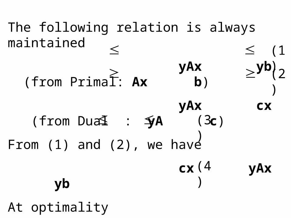
The following relation is always maintained

yAx yb (from Primal: Ax b)

yAx cx (from Dual : yA c)

From (1) and (2), we have

cx yAx yb

At optimality

cx* = y*Ax* = y*b

is always maintained.

(1)

(2)

(3)

(4)

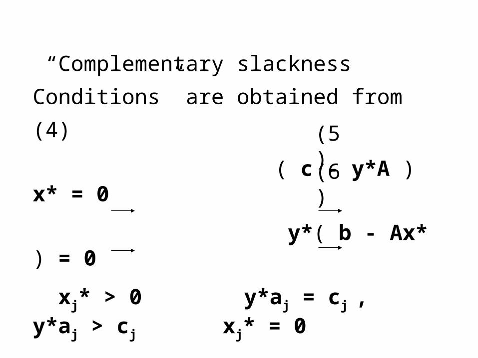
“Complementary slackness Conditions” are

obtained from (4)

( c - y*A ) x* = 0

y*( b - Ax* ) = 0

xj* > 0 y*aj = cj , y*aj > cj xj* = 0

yi* > 0 aix* = bi , ai x* < bi yi* = 0

(5)

(6)

Any pair of primal and dual problems can be

converted to each other.

The dual of a dual problem always is the primal

problem.

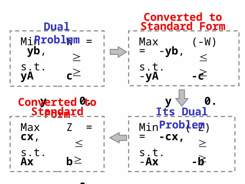
Min W = yb,

s.t. yA c

y 0.

Dual ProblemMax (-W) = -yb,

s.t. -yA -c

y 0.

Converted to Standard Form

Min (-Z) = -cx,

s.t. -Ax -b

x 0.

Its Dual Problem

Max Z = cx,

s.t. Ax b

x 0.

Converted toStandard Form

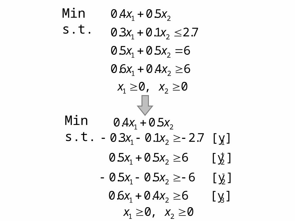
Mins.t.

64.06.0

65.05.0

7.21.03.0

21

21

21

xx

xx

xx

0,0 21 xx

21 5.04.0 xx

Mins.t.

][y 64.06.0

][y 65.05.0

][y 65.05.0

][y 7.21.03.0

321

-221

221

121

xx

xx

xx

xx

0,0 21 xx

21 5.04.0 xx

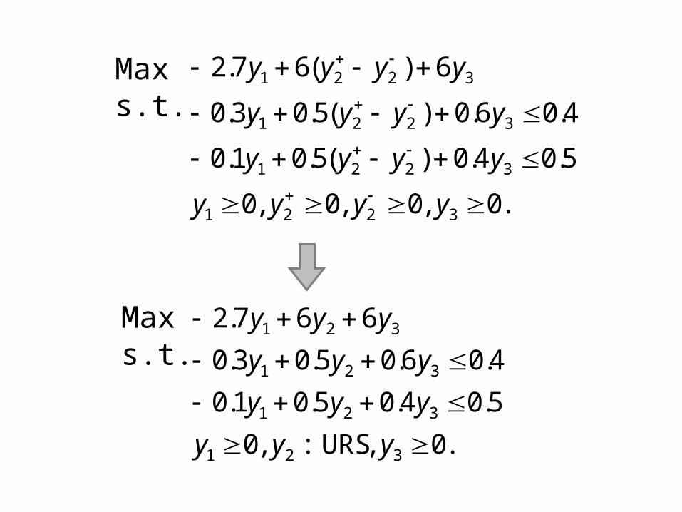
Maxs.t.

.0,0,0,0

5.04.0)(5.01.0

4.06.0)(5.03.0

6)(67.2

3221

3221

3221

3221

yyyy

yyyy

yyyy

yyyy

Maxs.t.

.0, URS:,0

5.04.05.01.0

4.06.05.03.0

667.2

321

321

321

321

yyy

yyy

yyy

yyy

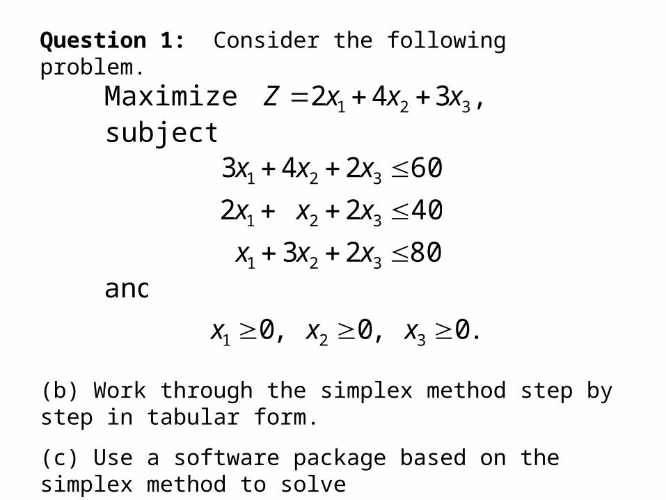
Question 1: Consider the following problem.

,342 Maximize 321 xxxZ

8023

4022

60243

321

321

321

xxx

xxx

xxxsubject to

and

.0,0,0 321 xxx

(b) Work through the simplex method step by step in tabular form.

(c) Use a software package based on the simplex method to solve

the problem.

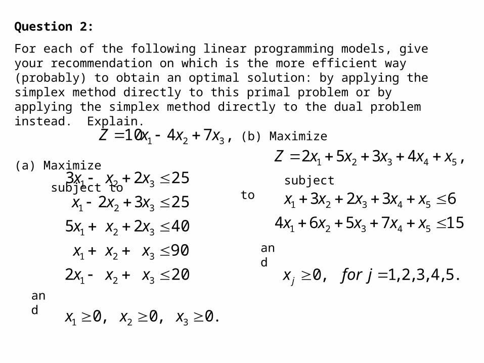
Question 2:

For each of the following linear programming models, give your recommendation on which is the more efficient way (probably) to obtain an optimal solution: by applying the simplex method directly to this primal problem or by applying the simplex method directly to the dual problem instead. Explain.

(a) Maximize

subject to

,7410 321 xxxZ

202

90

4025

2532

2523

321

321

321

321

321

xxx

xxx

xxx

xxx

xxx

and

.0,0,0 321 xxx

(b) Maximize

subject to

,4352 54321 xxxxxZ

157564

6323

54321

54321

xxxxx

xxxxx

and

.5,4,3,2,1,0 jforx j

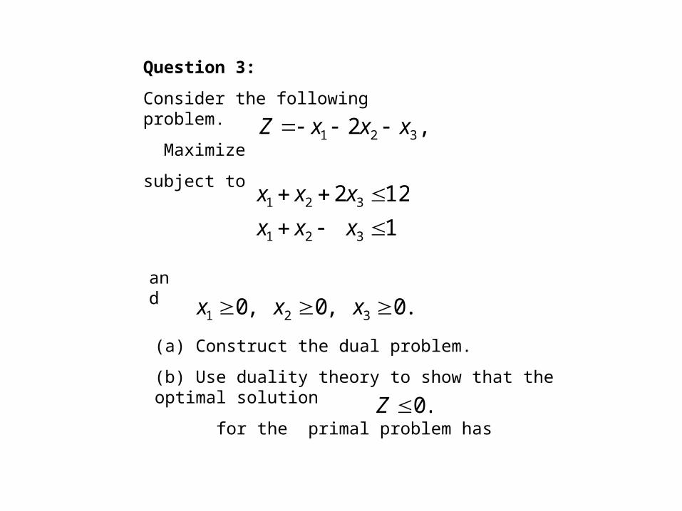
Question 3:

Consider the following problem.

Maximize

subject to

,2 321 xxxZ

1

122

321

321

xxx

xxx

and

.0,0,0 321 xxx

(a) Construct the dual problem.

(b) Use duality theory to show that the optimal solution

for the primal problem has .0Z