SANDIA REPORT

SAND2005-1107 Unlimited Release Printed March 2005 EMPHASIS/Nevada CABANA User Guide Version 1.0

C. David Turner

Prepared by Sandia National Laboratories Albuquerque, New Mexico 87185 and Livermore, California 94550 Sandia is a multiprogram laboratory operated by Sandia Corporation, a Lockheed Martin Company, for the United States Department of Energy�s National Nuclear Security Administration under Contract DE-AC04-94AL85000. Approved for public release; further dissemination unlimited.

Issued by Sandia National Laboratories, operated for the United States Department of Energy by Sandia Corporation.

NOTICE: This report was prepared as an account of work sponsored by an agency of the United States Government. Neither the United States Government, nor any agency thereof, nor any of their employees, nor any of their contractors, subcontractors, or their employees, make any warranty, express or implied, or assume any legal liability or responsibility for the accuracy, completeness, or usefulness of any information, apparatus, product, or process disclosed, or represent that its use would not infringe privately owned rights. Reference herein to any specific commercial product, process, or service by trade name, trademark, manufacturer, or otherwise, does not necessarily constitute or imply its endorsement, recommendation, or favoring by the United States Government, any agency thereof, or any of their contractors or subcontractors. The views and opinions expressed herein do not necessarily state or reflect those of the United States Government, any agency thereof, or any of their contractors. Printed in the United States of America. This report has been reproduced directly from the best available copy. Available to DOE and DOE contractors from

U.S. Department of Energy Office of Scientific and Technical Information P.O. Box 62 Oak Ridge, TN 37831 Telephone: (865)576-8401 Facsimile: (865)576-5728 E-Mail: reports@adonis.osti.gov Online ordering: http://www.osti.gov/bridge

Available to the public from

U.S. Department of Commerce National Technical Information Service 5285 Port Royal Rd Springfield, VA 22161 Telephone: (800)553-6847 Facsimile: (703)605-6900 E-Mail: orders@ntis.fedworld.gov Online order: http://www.ntis.gov/help/ordermethods.asp?loc=7-4-0#online

2

SAND2005-1107 Unlimited Release

Printed March 2005

EMPHASIS/Nevada CABANA User Guide Version 1.0

C. David Turner

Electromagnetics and Plasma Physics Analysis

Sandia National Laboratories P.O. Box 5800

Albuquerque, New Mexico 87185-1152

Abstract

The CABle ANAlysis (CABANA) portion of the EMPHASIS suite is designed specifically for the simulation of cable SGEMP. The code can be used to evaluate the response of a specific cable design to threat or to compare and minimize the relative response of difference designs. This document provides user-specific information to facilitate the application of the code to cables of interest.

3

Acknowledgement The author would like to thank all of those individuals who have helped to bring CABANA to the point it is today, including Gary Scrivner, Bill Bohnhoff, Wesley Fan, and Jennifer Powell for the CEPTRE interface.

4

Contents Acknowledgement ..............................................................................................4 Contents ..............................................................................................................5 List of Figures .....................................................................................................7 Introduction .........................................................................................................9 Cable SGEMP Simulation Process ....................................................................9 CABANA Input File and Keywords ..................................................................11

Time / time history keywords .......................................................................12 Radition-incidence keyword.........................................................................13 SPICE control keywords ...............................................................................14 Section keywords..........................................................................................15 CEPTRE data keywords ................................................................................15 Cable topology keywords .............................................................................17 Poisson solution keywords ..........................................................................18 Framework-related keywords within the physics block ............................19

Framework Keywords.......................................................................................20 Material-related keywords ............................................................................20 Simulation time and output control keywords............................................22 Linear solver keywords ................................................................................23

Follow-up Simulations with Stored Charge ....................................................23 Conclusion ........................................................................................................24 References ........................................................................................................25 Appendix I. CABANA output units ..................................................................27 Appendix II. Complete CABANA input file ......................................................28 Distribution........................................................................................................30

5

Intentionally Left Blank

6

List of Figures Figure 1. Cable-SGEMP Simulation Process.....................................................10 Figure 2. Typical CABANA physics keywords....................................................11 Figure 3. Non-normal incidence. ........................................................................13 Figure 4. Typical material model descriptions....................................................21 Figure 5. Typical simulation and output control keywords..................................22 Figure 6. Typical solver control keywords. .........................................................23

7

Intentionally Left Blank

8

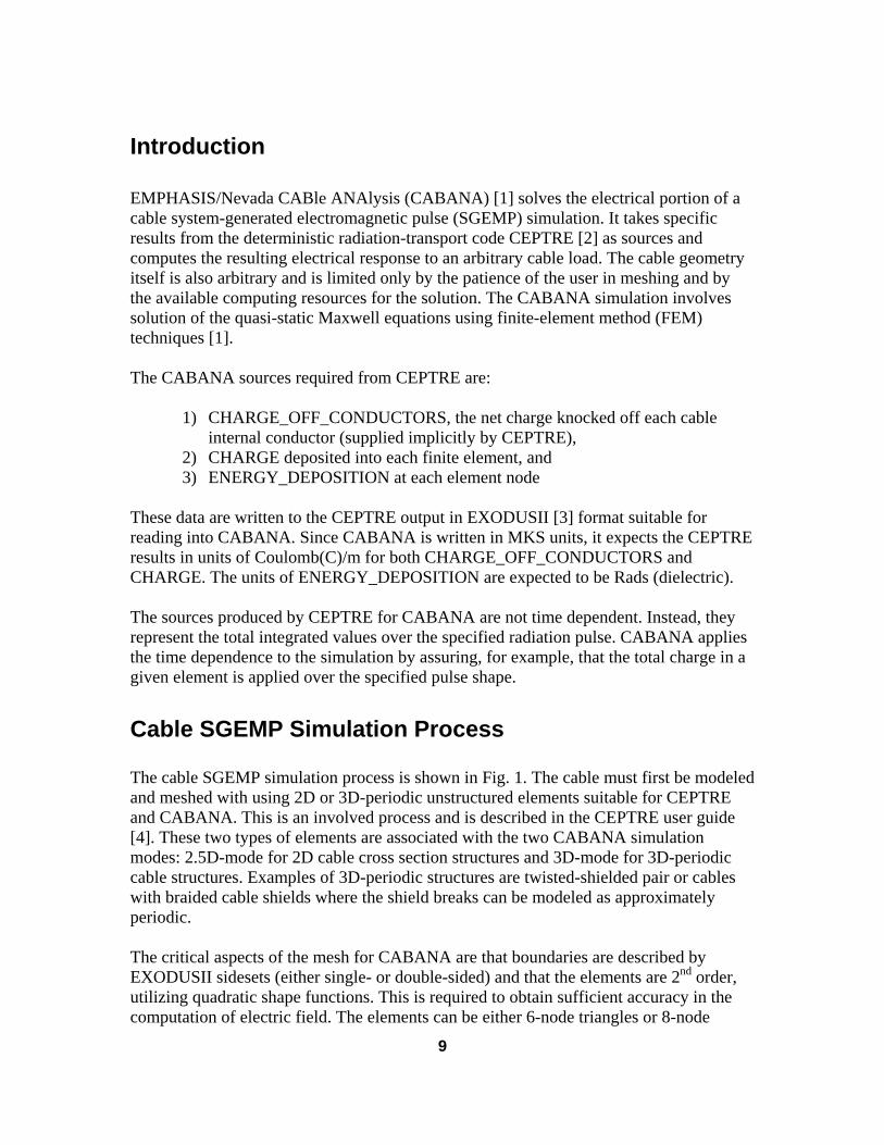
Introduction EMPHASIS/Nevada CABle ANAlysis (CABANA) [1] solves the electrical portion of a cable system-generated electromagnetic pulse (SGEMP) simulation. It takes specific results from the deterministic radiation-transport code CEPTRE [2] as sources and computes the resulting electrical response to an arbitrary cable load. The cable geometry itself is also arbitrary and is limited only by the patience of the user in meshing and by the available computing resources for the solution. The CABANA simulation involves solution of the quasi-static Maxwell equations using finite-element method (FEM) techniques [1]. The CABANA sources required from CEPTRE are:

1) CHARGE_OFF_CONDUCTORS, the net charge knocked off each cable internal conductor (supplied implicitly by CEPTRE),

2) CHARGE deposited into each finite element, and 3) ENERGY_DEPOSITION at each element node

These data are written to the CEPTRE output in EXODUSII [3] format suitable for reading into CABANA. Since CABANA is written in MKS units, it expects the CEPTRE results in units of Coulomb(C)/m for both CHARGE_OFF_CONDUCTORS and CHARGE. The units of ENERGY_DEPOSITION are expected to be Rads (dielectric). The sources produced by CEPTRE for CABANA are not time dependent. Instead, they represent the total integrated values over the specified radiation pulse. CABANA applies the time dependence to the simulation by assuring, for example, that the total charge in a given element is applied over the specified pulse shape.

Cable SGEMP Simulation Process The cable SGEMP simulation process is shown in Fig. 1. The cable must first be modeled and meshed with using 2D or 3D-periodic unstructured elements suitable for CEPTRE and CABANA. This is an involved process and is described in the CEPTRE user guide [4]. These two types of elements are associated with the two CABANA simulation modes: 2.5D-mode for 2D cable cross section structures and 3D-mode for 3D-periodic cable structures. Examples of 3D-periodic structures are twisted-shielded pair or cables with braided cable shields where the shield breaks can be modeled as approximately periodic. The critical aspects of the mesh for CABANA are that boundaries are described by EXODUSII sidesets (either single- or double-sided) and that the elements are 2nd order, utilizing quadratic shape functions. This is required to obtain sufficient accuracy in the computation of electric field. The elements can be either 6-node triangles or 8-node

9

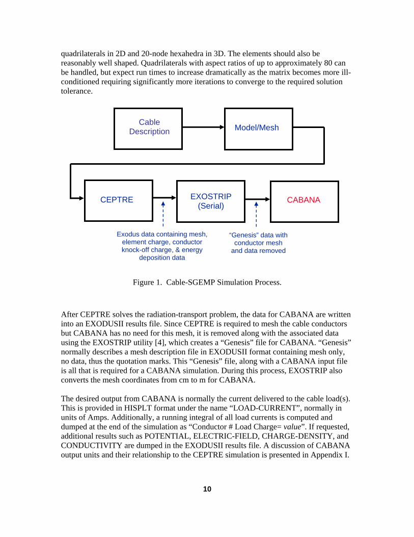
quadrilaterals in 2D and 20-node hexahedra in 3D. The elements should also be reasonably well shaped. Quadrilaterals with aspect ratios of up to approximately 80 can be handled, but expect run times to increase dramatically as the matrix becomes more ill-conditioned requiring significantly more iterations to converge to the required solution tolerance.

Cable Description Model/Mesh

CEPTRE EXOSTRIP (Serial)

CABANA

Exodus data containing mesh, element charge, conductor knock-off charge, & energy

deposition data

“Genesis” data with conductor mesh

and data removed

Figure 1. Cable-SGEMP Simulation Process.

After CEPTRE solves the radiation-transport problem, the data for CABANA are written into an EXODUSII results file. Since CEPTRE is required to mesh the cable conductors but CABANA has no need for this mesh, it is removed along with the associated data using the EXOSTRIP utility [4], which creates a “Genesis” file for CABANA. “Genesis” normally describes a mesh description file in EXODUSII format containing mesh only, no data, thus the quotation marks. This “Genesis” file, along with a CABANA input file is all that is required for a CABANA simulation. During this process, EXOSTRIP also converts the mesh coordinates from cm to m for CABANA. The desired output from CABANA is normally the current delivered to the cable load(s). This is provided in HISPLT format under the name “LOAD-CURRENT”, normally in units of Amps. Additionally, a running integral of all load currents is computed and dumped at the end of the simulation as “Conductor # Load Charge= value”. If requested, additional results such as POTENTIAL, ELECTRIC-FIELD, CHARGE-DENSITY, and CONDUCTIVITY are dumped in the EXODUSII results file. A discussion of CABANA output units and their relationship to the CEPTRE simulation is presented in Appendix I.

10

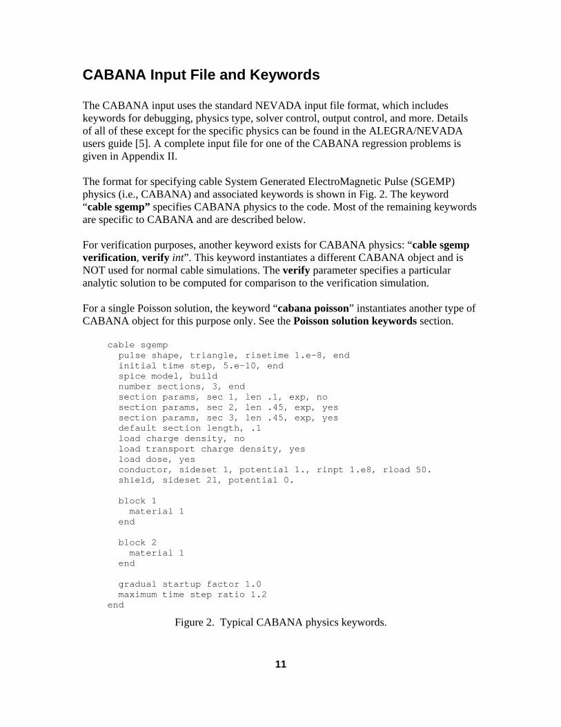
CABANA Input File and Keywords The CABANA input uses the standard NEVADA input file format, which includes keywords for debugging, physics type, solver control, output control, and more. Details of all of these except for the specific physics can be found in the ALEGRA/NEVADA users guide [5]. A complete input file for one of the CABANA regression problems is given in Appendix II. The format for specifying cable System Generated ElectroMagnetic Pulse (SGEMP) physics (i.e., CABANA) and associated keywords is shown in Fig. 2. The keyword “cable sgemp” specifies CABANA physics to the code. Most of the remaining keywords are specific to CABANA and are described below. For verification purposes, another keyword exists for CABANA physics: “cable sgemp verification, verify int”. This keyword instantiates a different CABANA object and is NOT used for normal cable simulations. The verify parameter specifies a particular analytic solution to be computed for comparison to the verification simulation. For a single Poisson solution, the keyword “cabana poisson” instantiates another type of CABANA object for this purpose only. See the Poisson solution keywords section.

cable sgemp pulse shape, triangle, risetime 1.e-8, end initial time step, 5.e-10, end spice model, build number sections, 3, end section params, sec 1, len .1, exp, no section params, sec 2, len .45, exp, yes section params, sec 3, len .45, exp, yes default section length, .1 load charge density, no load transport charge density, yes load dose, yes conductor, sideset 1, potential 1., rinpt 1.e8, rload 50. shield, sideset 21, potential 0. block 1 material 1 end block 2 material 1 end gradual startup factor 1.0 maximum time step ratio 1.2 end

Figure 2. Typical CABANA physics keywords.

11

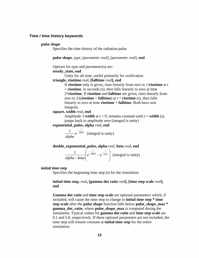
Time / time history keywords

pulse shape Specifies the time history of the radiation pulse pulse shape, type, [parameter real], [parameter real], end Options for type and parameter(s) are: steady_state, end

Unity for all time, useful primarily for verification triangle, risetime real, [falltime real], end

If risetime only is given, rises linearly from zero to 1/risetime at t = risetime, in seconds (s), then falls linearly to zero at time 2*risetime. If risetime and falltime are given, rises linearly from zero to 2/(risetime + falltime) at t = risetime (s), then falls linearly to zero at time risetime + falltime. Both have unit integrals.

square, width real, end Amplitude 1/width at t = 0, remains constant until t = width (s), jumps back to amplitude zero (integral is unity)

exponential_pulse, alpha real, end

alphat

ealpha

−1 (integral is unity)

double_exponential_pulse, alpha real, beta real, end

⎟⎟⎠

⎞⎜⎜⎝

⎛−

−

−−beta

talpha

t

eebetaalpha

1 (integral is unity)

initial time step

Specifies the beginning time step (s) for the simulation initial time step, real, [gamma dot ratio real], [time step scale real], end Gamma dot ratio and time step scale are optional parameters which, if included, will cause the time step to change to initial time step * time step scale after the pulse shape function falls below pulse_shape_max * gamma_dot_ratio, where pulse_shape_max is computed during the simulation. Typical values for gamma dot ratio and time step scale are 0.1 and 5.0, respectively. If these optional parameters are not included, the time step will remain constant at initial time step for the entire simulation.

12

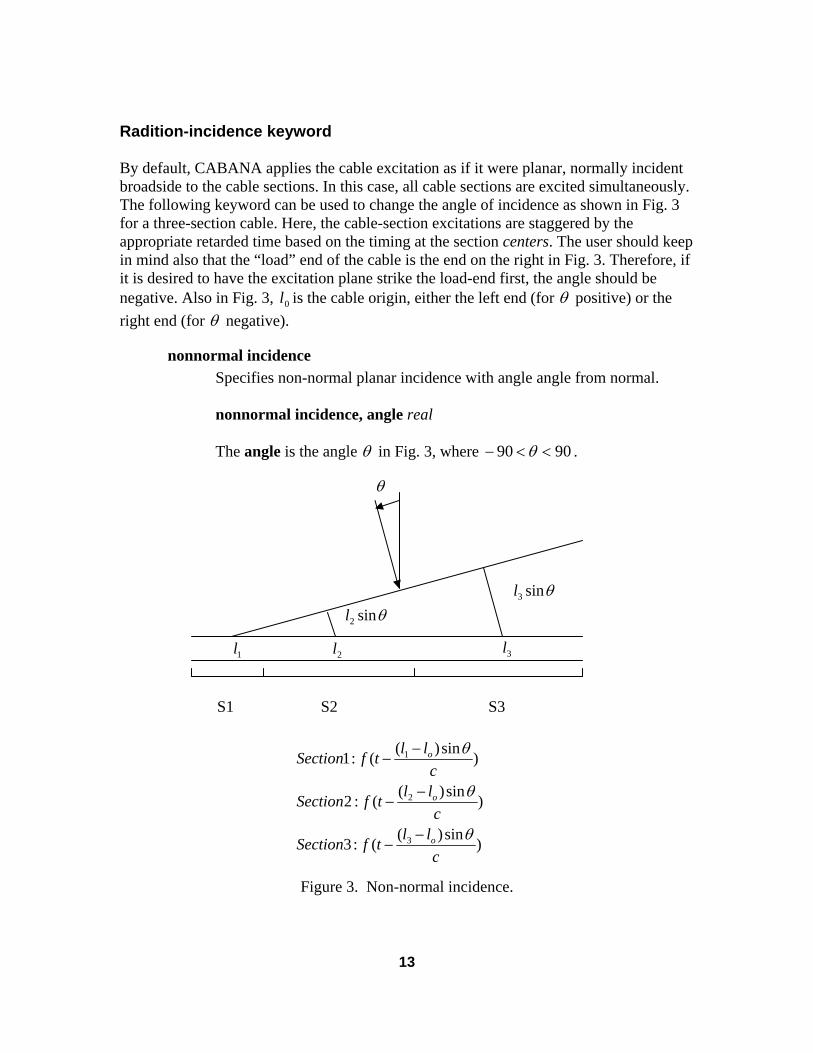
Radition-incidence keyword By default, CABANA applies the cable excitation as if it were planar, normally incident broadside to the cable sections. In this case, all cable sections are excited simultaneously. The following keyword can be used to change the angle of incidence as shown in Fig. 3 for a three-section cable. Here, the cable-section excitations are staggered by the appropriate retarded time based on the timing at the section centers. The user should keep in mind also that the “load” end of the cable is the end on the right in Fig. 3. Therefore, if it is desired to have the excitation plane strike the load-end first, the angle should be negative. Also in Fig. 3, is the cable origin, either the left end (for 0l θ positive) or the right end (for θ negative).

nonnormal incidence Specifies non-normal planar incidence with angle angle from normal. nonnormal incidence, angle real

The angle is the angle θ in Fig. 3, where 9090 <<− θ .

S1 S2 S3

θ

θsin2lθsin3l

)sin)((:3

)sin)((:2

)sin)((:1

3

2

1

clltfSection

clltfSection

clltfSection

o

o

o

θ

θ

θ

−−

−−

−−

2l1l 3l

Figure 3. Non-normal incidence.

13

SPICE control keywords

spice model Specifies how SPICE is utilized and the origin of the spice model deck for the simulation spice model, spice_option Options for spice_option are: NO

SPICE not used in simulation USE

Lumped-parameter SPICE deck will be read from file BUILD

Lumped-parameter SPICE deck will be created and written to a file during startup

Generally, the initial simulation for a given cable geometry is accomplished using the BUILD option which writes the SPICE deck to a file (see spice file keyword below). If custom changes are desired to this SPICE model for subsequent simulations, the file can be edited and the USE option invoked thereafter.

spice file

Specifies the filename from which to read the SPICE model deck if “spice model, USE” is specified or the file to which to write the SPICE deck if “spice model, BUILD” is specified. spice file, “filename” filename is an asci string and the quotes are required. If spice file is not specified, the SPICE deck is either read from or written to the default filename problem_name.in. Note that this file, either the default or that specified by spice file, will be OVERWRITTEN for the next simulation if it is left in place on the file system.

spice step fraction

Specifies the fraction of the initial time step (see initial time step keyword) which SPICE will use as a maximum internal time step. spice step fraction, real The default is 0.1. In some cases, it is necessary to increase this value to something like 0.5 to allow SPICE to converge correctly. If such a SPICE

14

error occurs, the error is trapped and the user is notified to modify this value.

Section keywords number sections

Specifies the number of sections to divide the cable length into for a 2.5D simulation and optionally specifies the lengths of each section. However, for a large number of sections, the line length may exceed the maximum. In this case, use multiple of the below section params keywords. number sections, int, [sec int, len real], [sec int, len real], […], end Each [sec int, len real] specifies the section number and length, in meters (m), of one of the sections. If a section is not specified, its’ length is defined by the default section length keyword below. In addition, it will be exposed to radiation by default (see section params below).

section params

Optionally specifies the lengths of each section and whether the section is exposed to radiation. The length parameter can be specified with the number sections keyword above if desired. section params, sec[tion] int, len[gth] real, exp[osed], bool Each keyword of this type specifies the section number and length (m) of one section. Options for the exp parameter are “YES” (or “TRUE”) and “NO” (or “FALSE”). Note that the comma after exp must be present. If a section is not specified, its’ length is defined by the default section length keyword below and exp is “YES”.

default section length Specifies the default length (m) of each cable section default section length, real

CEPTRE data keywords

load charge density Specifies whether the CEPTRE data for CHARGE density contained in the simulation genesis file is loaded before the first time cycle

15

load charge density, option Options for option are: NO (default)

CHARGE not loaded up front, typical for actual cable simulation

YES CHARGE loaded up front, typical for verification simulation

load transport charge density

Specifies whether CEPTRE data for CHARGE density contained in the simulation genesis file is prepared for loading into the simulation over the radiation pulse defined by pulse shape load transport charge density, option Options for option are: YES (default)

CHARGE prepared for loading, typical for actual cable simulation

NO CHARGE not prepared for loading, typical for verification simulation

load dose

Specifies whether CEPTRE data for ENERGY_DEPOSITION contained in the simulation genesis file is prepared for loading into the simulation over the radiation pulse defined by pulse shape load dose, option Options for option are: YES (default)

ENERGY_DEPOSITION prepared for loading, typical for actual cable simulation

NO ENERGY_DEPOSITION not prepared for loading, typical for verification simulation or for turning off radiation induced conductivity (RIC)

16

Cable topology keywords

conductor

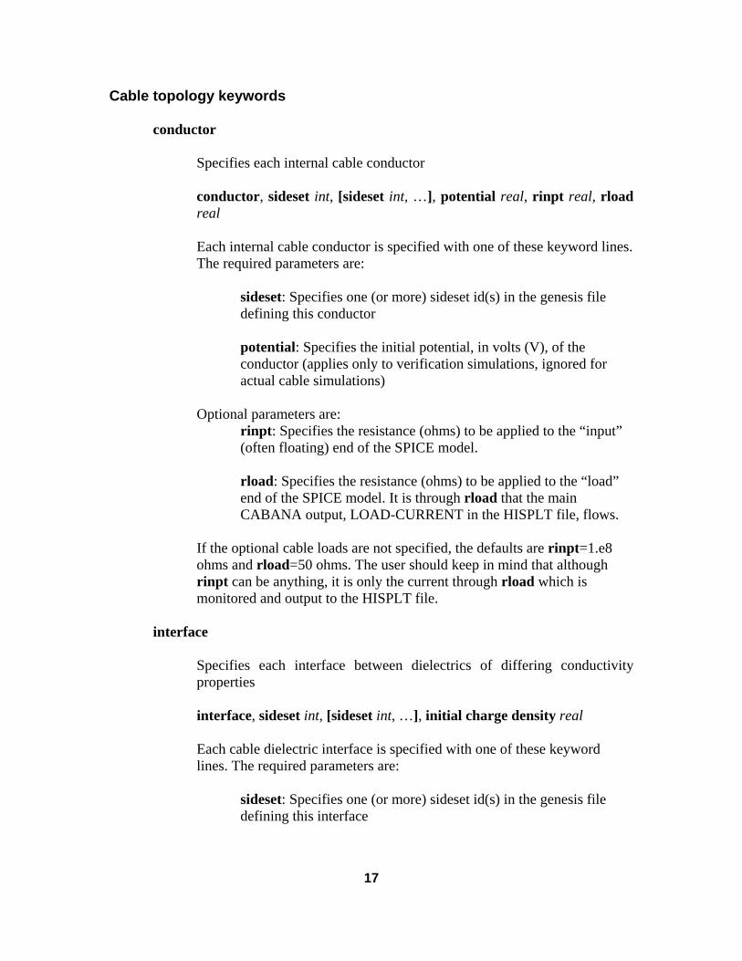
Specifies each internal cable conductor conductor, sideset int, [sideset int, …], potential real, rinpt real, rload real Each internal cable conductor is specified with one of these keyword lines. The required parameters are:

sideset: Specifies one (or more) sideset id(s) in the genesis file defining this conductor potential: Specifies the initial potential, in volts (V), of the conductor (applies only to verification simulations, ignored for actual cable simulations)

Optional parameters are: rinpt: Specifies the resistance (ohms) to be applied to the “input” (often floating) end of the SPICE model. rload: Specifies the resistance (ohms) to be applied to the “load” end of the SPICE model. It is through rload that the main CABANA output, LOAD-CURRENT in the HISPLT file, flows.

If the optional cable loads are not specified, the defaults are rinpt=1.e8 ohms and rload=50 ohms. The user should keep in mind that although rinpt can be anything, it is only the current through rload which is monitored and output to the HISPLT file.

interface

Specifies each interface between dielectrics of differing conductivity properties interface, sideset int, [sideset int, …], initial charge density real Each cable dielectric interface is specified with one of these keyword lines. The required parameters are:

sideset: Specifies one (or more) sideset id(s) in the genesis file defining this interface

17

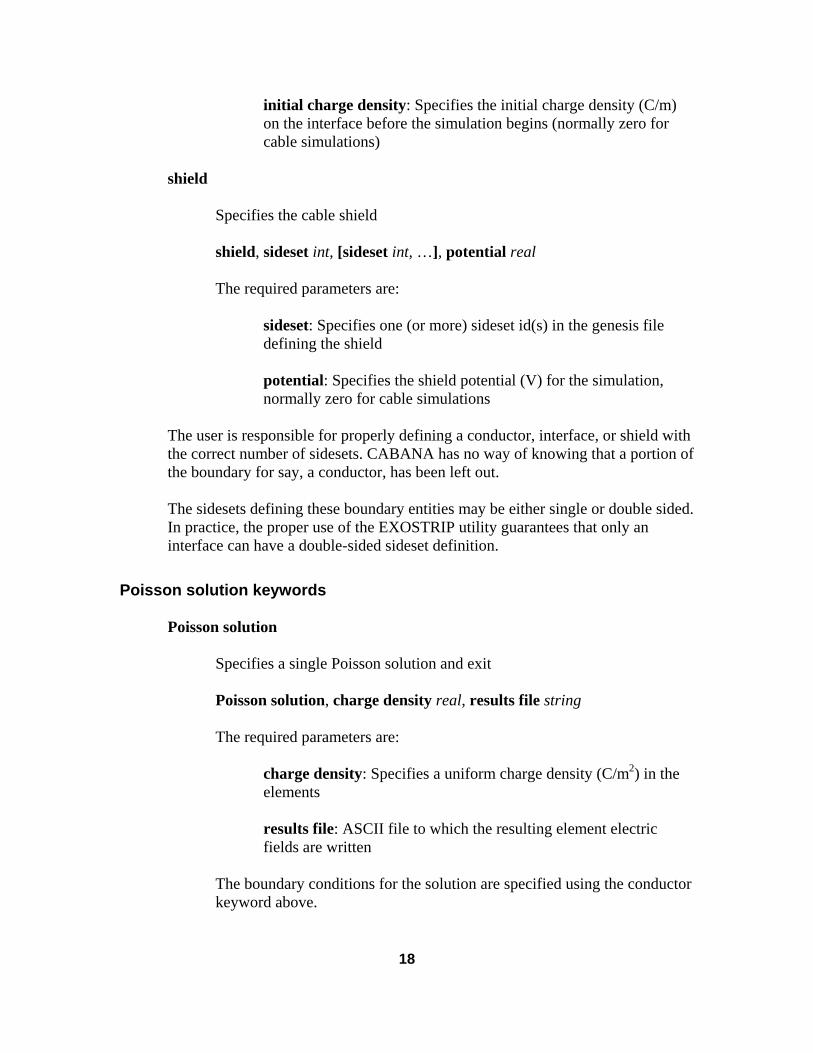
initial charge density: Specifies the initial charge density (C/m) on the interface before the simulation begins (normally zero for cable simulations)

shield

Specifies the cable shield shield, sideset int, [sideset int, …], potential real The required parameters are:

sideset: Specifies one (or more) sideset id(s) in the genesis file defining the shield potential: Specifies the shield potential (V) for the simulation, normally zero for cable simulations

The user is responsible for properly defining a conductor, interface, or shield with the correct number of sidesets. CABANA has no way of knowing that a portion of the boundary for say, a conductor, has been left out. The sidesets defining these boundary entities may be either single or double sided. In practice, the proper use of the EXOSTRIP utility guarantees that only an interface can have a double-sided sideset definition.

Poisson solution keywords

Poisson solution

Specifies a single Poisson solution and exit Poisson solution, charge density real, results file string The required parameters are:

charge density: Specifies a uniform charge density (C/m2) in the elements results file: ASCII file to which the resulting element electric fields are written

The boundary conditions for the solution are specified using the conductor keyword above.

18

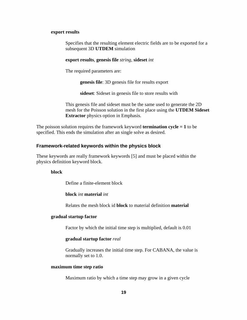
export results

Specifies that the resulting element electric fields are to be exported for a subsequent 3D UTDEM simulation export results, genesis file string, sideset int The required parameters are:

genesis file: 3D genesis file for results export sideset: Sideset in genesis file to store results with

This genesis file and sideset must be the same used to generate the 2D mesh for the Poisson solution in the first place using the UTDEM Sideset Extractor physics option in Emphasis.

The poisson solution requires the framework keyword termination cycle = 1 to be specified. This ends the simulation after an single solve as desired.

Framework-related keywords within the physics block These keywords are really framework keywords [5] and must be placed within the physics definition keyword block.

block

Define a finite-element block block int material int Relates the mesh block id block to material definition material

gradual startup factor

Factor by which the initial time step is multiplied, default is 0.01

gradual startup factor real Gradually increases the initial time step. For CABANA, the value is normally set to 1.0.

maximum time step ratio

Maximum ratio by which a time step may grow in a given cycle

19

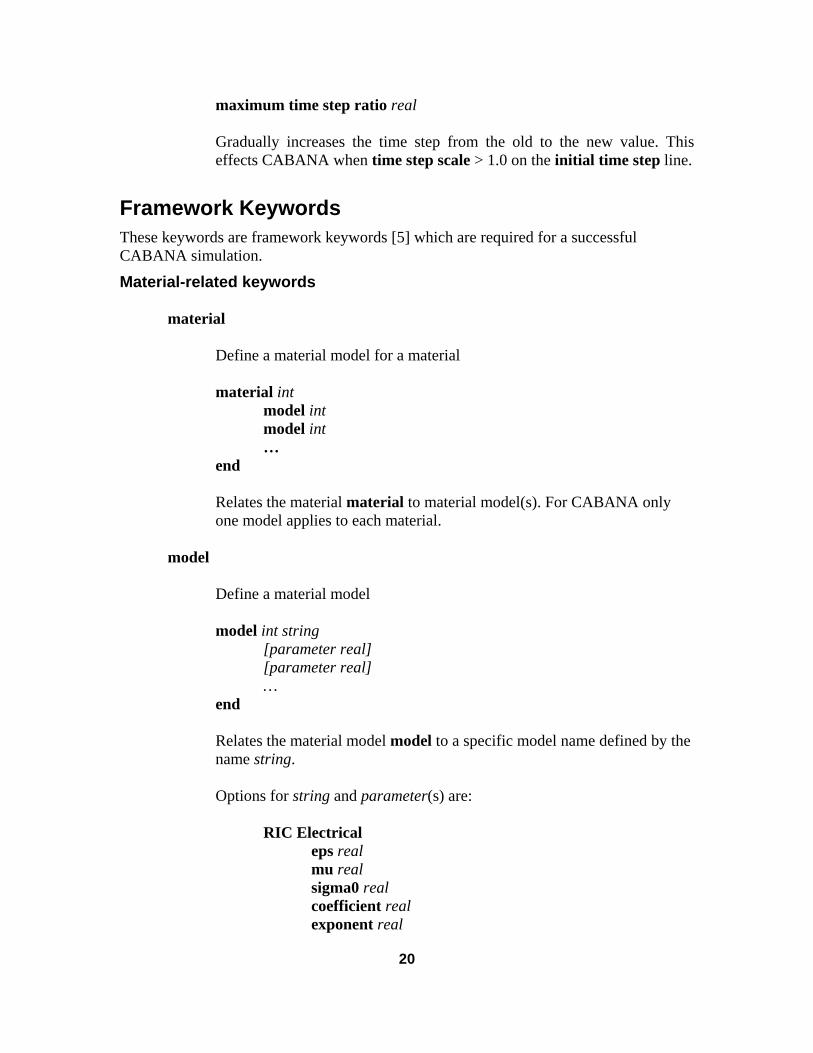
maximum time step ratio real Gradually increases the time step from the old to the new value. This effects CABANA when time step scale > 1.0 on the initial time step line.

Framework Keywords These keywords are framework keywords [5] which are required for a successful CABANA simulation.

Material-related keywords

material

Define a material model for a material material int

model int model int …

end Relates the material material to material model(s). For CABANA only one model applies to each material.

model

Define a material model model int string

[parameter real] [parameter real] …

end Relates the material model model to a specific model name defined by the name string. Options for string and parameter(s) are:

RIC Electrical eps real mu real sigma0 real coefficient real exponent real

20

end or

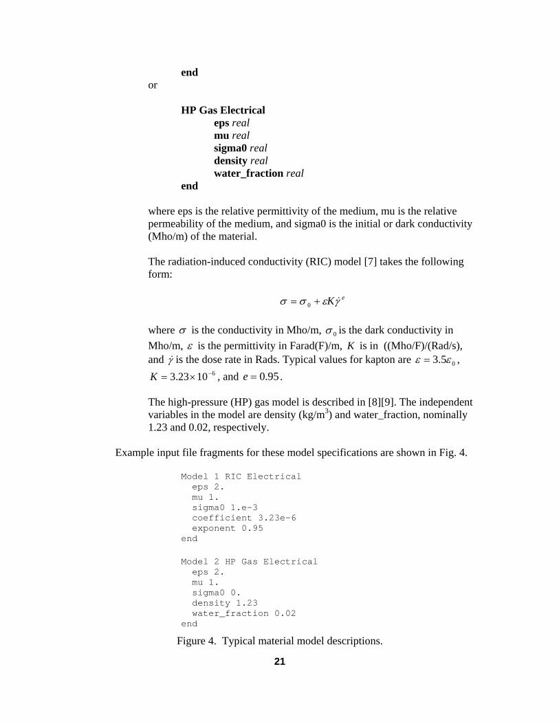
HP Gas Electrical eps real mu real sigma0 real density real water_fraction real

end

where eps is the relative permittivity of the medium, mu is the relative permeability of the medium, and sigma0 is the initial or dark conductivity (Mho/m) of the material. The radiation-induced conductivity (RIC) model [7] takes the following form:

eKγεσσ &+= 0 where σ is the conductivity in Mho/m, 0σ is the dark conductivity in Mho/m, ε is the permittivity in Farad(F)/m, K is in ((Mho/F)/(Rad/s), and γ& is the dose rate in Rads. Typical values for kapton are 05.3 εε = ,

, and 61023.3 −×=K 95.0=e . The high-pressure (HP) gas model is described in [8][9]. The independent variables in the model are density (kg/m3) and water_fraction, nominally 1.23 and 0.02, respectively.

Example input file fragments for these model specifications are shown in Fig. 4.

Model 1 RIC Electrical eps 2. mu 1. sigma0 1.e-3 coefficient 3.23e-6 exponent 0.95 end

Model 2 HP Gas Electrical eps 2. mu 1. sigma0 0. density 1.23 water_fraction 0.02 end

Figure 4. Typical material model descriptions.

21

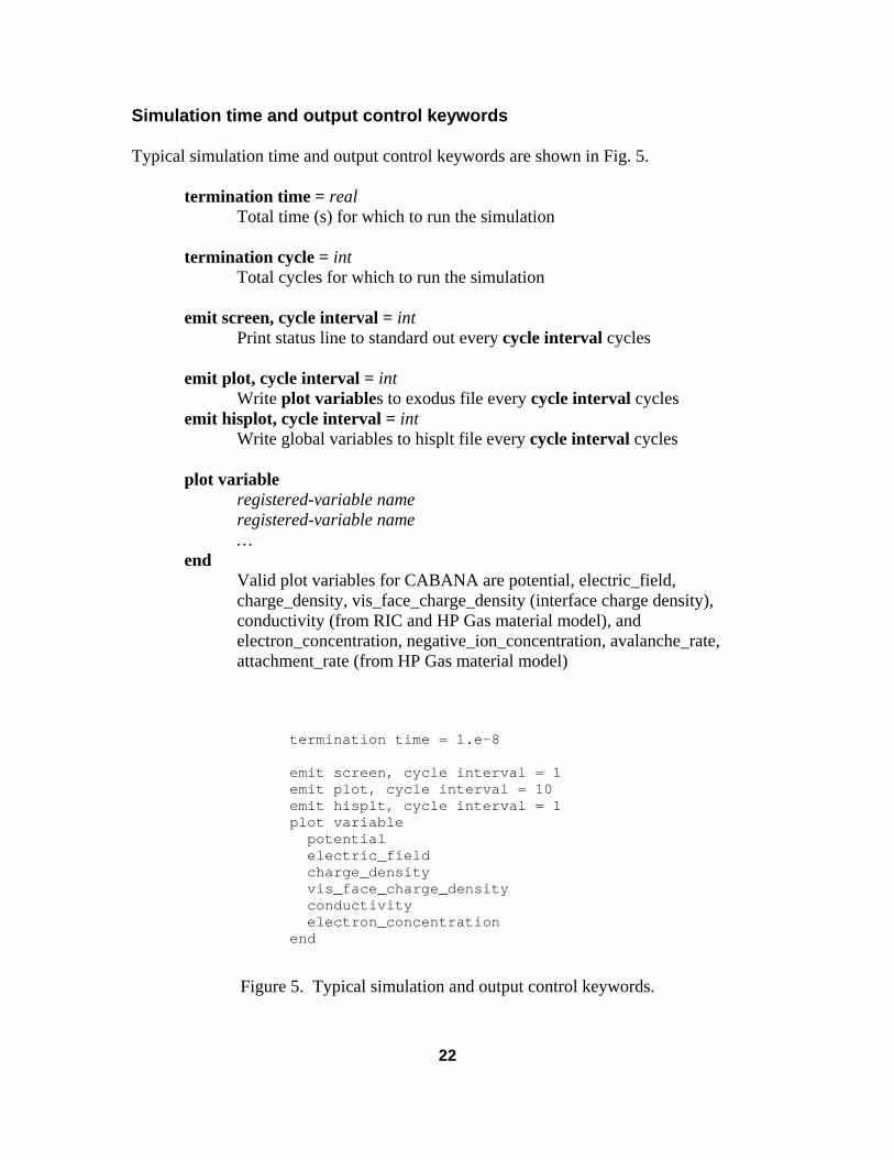
Simulation time and output control keywords Typical simulation time and output control keywords are shown in Fig. 5.

termination time = real Total time (s) for which to run the simulation

termination cycle = int Total cycles for which to run the simulation

emit screen, cycle interval = int

Print status line to standard out every cycle interval cycles

emit plot, cycle interval = int Write plot variables to exodus file every cycle interval cycles

emit hisplot, cycle interval = int Write global variables to hisplt file every cycle interval cycles

plot variable registered-variable name registered-variable name …

end Valid plot variables for CABANA are potential, electric_field, charge_density, vis_face_charge_density (interface charge density), conductivity (from RIC and HP Gas material model), and electron_concentration, negative_ion_concentration, avalanche_rate, attachment_rate (from HP Gas material model)

termination time = 1.e-8 emit screen, cycle interval = 1 emit plot, cycle interval = 10 emit hisplt, cycle interval = 1 plot variable potential electric_field charge_density vis_face_charge_density conductivity electron_concentration end

Figure 5. Typical simulation and output control keywords.

22

If plot variables are not desired the “emit plot” line can be omitted. If plot variables are desired but not at frequent intervals, the cycle interval should be set to large values to avoid exceedingly large exodus files.

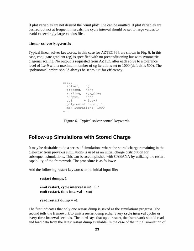
Linear solver keywords Typical linear solver keywords, in this case for AZTEC [6], are shown in Fig. 6. In this case, conjugate gradient (cg) is specified with no preconditioning but with symmetric diagonal scaling. No output is requested from AZTEC after each solve to a tolerance level of 1.e-9 with a maximum number of cg iterations set to 1000 (default is 500). The “polynomial order” should always be set to “1” for efficiency.

aztec solver, cg precond, none scaling, sym_diag output, none tol = 1.e-9 polynomial order, 1 max iterations, 1000 end

Figure 6. Typical solver control keywords.

Follow-up Simulations with Stored Charge It may be desirable to do a series of simulations where the stored charge remaining in the dielectric from previous simulations is used as an initial charge distribution for subsequent simulations. This can be accomplished with CABANA by utilizing the restart capability of the framework. The procedure is as follows: Add the following restart keywords to the initial input file:

restart dumps, 1 emit restart, cycle interval = int OR emit restart, time interval = real read restart dump = –1

The first indicates that only one restart dump is saved as the simulations progress. The second tells the framework to emit a restart dump either every cycle interval cycles or every time interval seconds. The third says that upon restart, the framework should read and load data from the latest restart dump available. In the case of the initial simulation of

23

the series, the user should verify that no restart dumps exist in the directory and the simulation will then start at time=0. as desired. Restart dumps are written to files in the format: problem_name.dmp.restart_number. For subsequent simulations, the user must change the termination time to have a later termination time for the next simulation. With this change, the follow-on simulation will begin at the time of the final restart dump from the previous simulation after loading the residual dielectric charge. In addition, the original gen file can be optionally replaced at this time with a new one having the identical mesh description but containing a different set of radiation-transport results. The user is also free to change other simulation parameters such as pulse shape, time step, etc. A key assumption in this process is that the SPICE circuit model is completely discharged after each simulation in the series, since no SPICE state is saved. This requires that each simulation be run until such time as this is essentially the case, i.e., all cable reflections have subsided and a reasonably steady-state condition has been reached.

Conclusion This document, along with the user guides for a modeling and meshing tool such as I-DEAS, the radiation-transport code CEPTRE, and the exodus-file stripping tool EXOSTRIP should allow the user to successfully utilize CABANA to simulate the cable SGEMP response of an arbitrary cable geometry. To gain experience, the CABANA regression suite contains several realistic cable simulations, both 2.5D and 3D. Although these do not have realistic radiation-transport data in their Genesis files, the data does adequately exercise the algorithms in the code and fully demonstrates the cable simulation.

24

References 1. C. D. Turner and G. J. Scrivner, CABANA Serial/Development Version Description,

Verification, and Validation, Sandia National Laboratories Report SAND2001-3567, Nov. 2001.

2. C. R. Drumm, Parallel Finite Element Electron-Photon Transport Analysis on 2-D

Unstructured Mesh, Sandia National Laboratories Report SAND99-0098, Jan. 1999. 3. L. A. Schoof, V. R. Yarberry, EXODUSII: A Finite Element Data Model, Sandia

National Laboratories Report SAND92-2137, reprinted Sep. 1996. 4. J. L. Powell, A Users Manual for CEPTRE in the Nevada Framework, Sandia

National Laboratories Report SAND2004-xxxx, July 2004. 5. E. A. Boucheron, et. al., ALEGRA: User Input and Physics Descriptions- OCT 99

Release, Sandia National Laboratories Report SAND99-3012, Dec. 1999. 6. R. S. Tuminaro, M. Heroux, S. A. Hutchinson, J. N. Shadid, Official Aztec User’s

Guide Version 2.1, Sandia National Laboratories Report SAND99-8801J, Nov. 1999. 7. Steven Face, Cable Response Parameter Determination, K-87-32U(R), Kaman

Sciences Corporation, Colorado Springs, CO, April 1987. 8. Tom Stringer, ITT Corp., private communication. 9. Tumolillo and Wondra, PRES 3D: A Computer Code for the Self Consistent Solution

of the Maxwell Lorentz Three Species Air Chemistry Equations in Three D., IEEE Trans. Nucl. Sci., Vol NS-24, No. 6, Dec. 1977, pgs 2456-2460.

25

Intentionally Left Blank

26

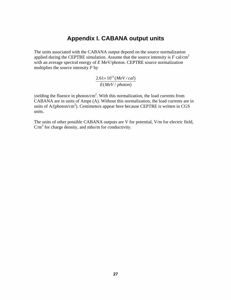
Appendix I. CABANA output units The units associated with the CABANA output depend on the source normalization applied during the CEPTRE simulation. Assume that the source intensity is F cal/cm2 with an average spectral energy of E MeV/photon. CEPTRE source normalization multiplies the source intensity F by

)/()/(1061.2 13

photonMeVEcalMeV×

yielding the fluence in photon/cm2. With this normalization, the load currents from CABANA are in units of Amps (A). Without this normalization, the load currents are in units of A/(photon/cm2). Centimeters appear here because CEPTRE is written in CGS units. The units of other possible CABANA outputs are V for potential, V/m for electric field, C/m3 for charge density, and mho/m for conductivity.

27

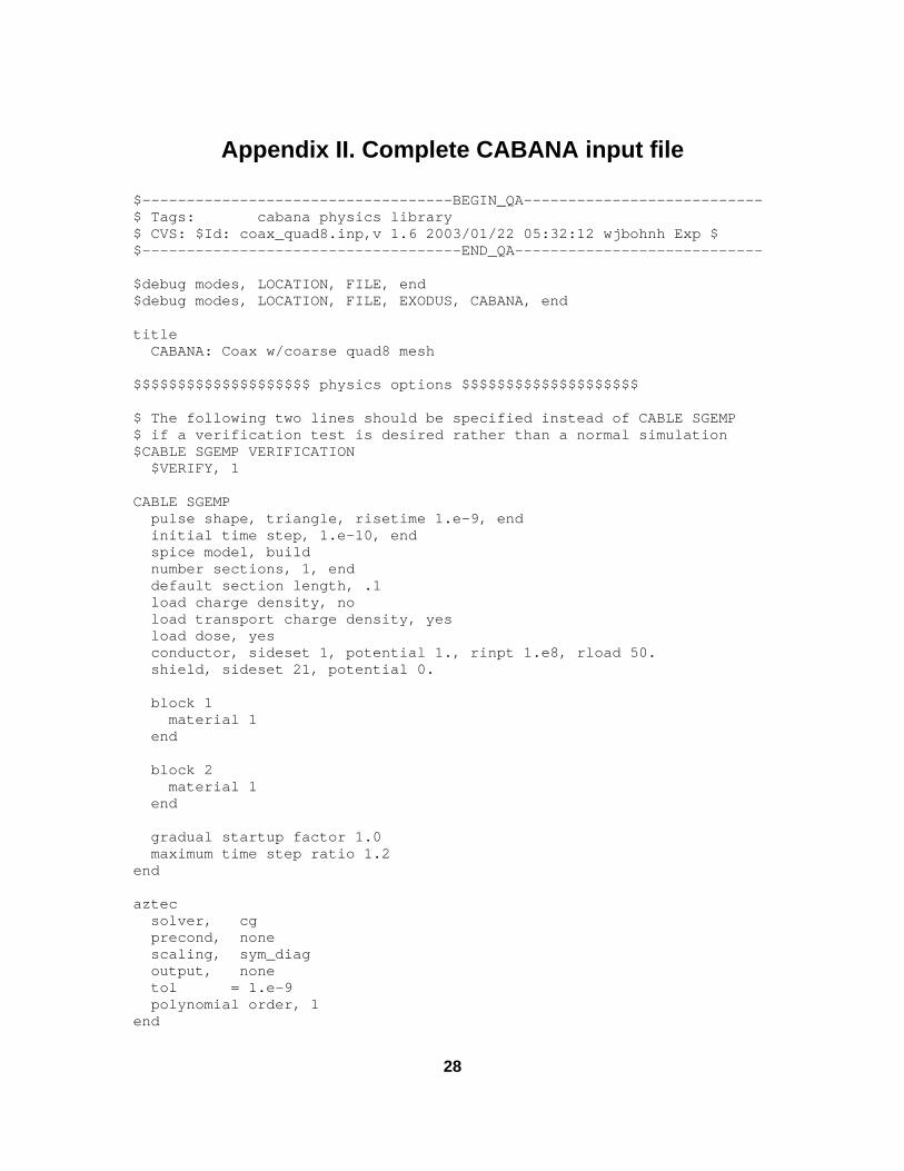
Appendix II. Complete CABANA input file $-----------------------------------BEGIN_QA--------------------------- $ Tags: cabana physics library $ CVS: $Id: coax_quad8.inp,v 1.6 2003/01/22 05:32:12 wjbohnh Exp $ $------------------------------------END_QA---------------------------- $debug modes, LOCATION, FILE, end $debug modes, LOCATION, FILE, EXODUS, CABANA, end title CABANA: Coax w/coarse quad8 mesh $$$$$$$$$$$$$$$$$$$$ physics options $$$$$$$$$$$$$$$$$$$$ $ The following two lines should be specified instead of CABLE SGEMP $ if a verification test is desired rather than a normal simulation $CABLE SGEMP VERIFICATION $VERIFY, 1 CABLE SGEMP pulse shape, triangle, risetime 1.e-9, end initial time step, 1.e-10, end spice model, build number sections, 1, end default section length, .1 load charge density, no load transport charge density, yes load dose, yes conductor, sideset 1, potential 1., rinpt 1.e8, rload 50. shield, sideset 21, potential 0. block 1 material 1 end block 2 material 1 end gradual startup factor 1.0 maximum time step ratio 1.2 end aztec solver, cg precond, none scaling, sym_diag output, none tol = 1.e-9 polynomial order, 1 end

28

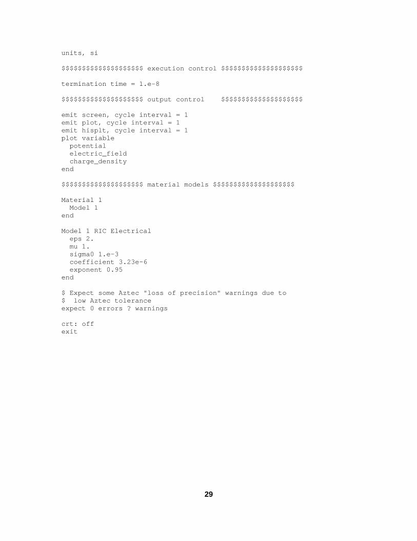
units, si $$$$$$$$$$$$$$$$$$$$ execution control $$$$$$$$$$$$$$$$$$$$ termination time = 1.e-8 $$$$$$$$$$$$$$$$$$$$ output control $$$$$$$$$$$$$$$$$$$$ emit screen, cycle interval = 1 emit plot, cycle interval = 1 emit hisplt, cycle interval = 1 plot variable potential electric_field charge_density end $$$$$$$$$$$$$$$$$$$$ material models $$$$$$$$$$$$$$$$$$$$ Material 1 Model 1 end Model 1 RIC Electrical eps 2. mu 1. sigma0 1.e-3 coefficient 3.23e-6 exponent 0.95 end $ Expect some Aztec "loss of precision" warnings due to $ low Aztec tolerance expect 0 errors ? warnings crt: off exit

29

Distribution 1 MS1152 M. L. Kiefer, 01642 5 MS1152 C. D. Turner, 01642 1 MS0437 J. R. Lee, 06700 1 MS1179 L. Lorence, 06741 1 MS1179 J. L. Powell, 06741 1 MS1167 E. F. Hartman, 06743 1 MS1159 M. A. Hedemann, 06744 1 MS1166 G. J. Scrivner, 06745 1 MS1166 C. R. Drumm, 06745 1 MS1166 W. C. Fan, 06745 1 MS9153 W. P. Ballard, 08200 1 MS0378 W. J. Bohnhoff, 09231 1 MS9018 Central Technical File, 8945-1 2 MS0899 Technical Library, 9616

30