empirical methods - wharton...

1 Copyright © Michael R. Roberts

Regression Discontinuity Design (RDD)

Empirical Methods

Prof. Michael R. Roberts


Topic Overview

  Introduction »  Intuition »  An early example »  Some nice features of RDD

  RDD »  Sharp RDD »  Fuzzy RDD

  Implementation »  Graphical Analysis »  Estimation »  Sensitivity Analysis

  Extensions   References


RDD Intuition

  RDD is a quasi-experimental technique »  Assignment to treatment and control is not random

–  Treatment and Control groups may differ systematically in ways related to the outcome…not good because then outcome may not be due to treatment

»  But, we know the assignment rule influencing how people are assigned or selected in to treatment –  There is a known cut-off in treatment assignment or in probability

of treatment receipt as a function of one or more continuous variables that generates a discontinuity in the treatment recipiency rate at that point


RDD Example Thistlethwaite and Campbell (1960)

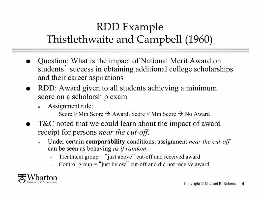
  Question: What is the impact of National Merit Award on students’ success in obtaining additional college scholarships and their career aspirations

  RDD: Award given to all students achieving a minimum score on a scholarship exam »  Assignment rule:

–  Score ≥ Min Score Award; Score < Min Score No Award

  T&C noted that we could learn about the impact of award receipt for persons near the cut-off. »  Under certain comparability conditions, assignment near the cut-off

can be seen as behaving as if random. –  Treatment group = “just above” cut-off and received award –  Control group = “just below” cut-off and did not receive award


Some Nice Features of RDD

1.  RDDs abound once you looked for them »  Program resources often allocated based on a formula with a cut-off

structure –  Allocate scarce resources to those who need or deserve

2.  RDD is intuitive and easily conveyed by a picture showing sharp changes in »  treatment assignment, and »  average outcomes

around cut-off value of assignment variable 3.  There are several different ways to estimate the treatment

effect, each of which have credible causal interpretations


Notation

  yi(1) = outcome of person i given treatment   yi(0) = outcome of person i in absence of treatment   Interest lies in yi(1) - yi(0) = effect of treatment on subject i

»  Can vary across i   yi(1) and yi(0) are the pair of potential outcomes for unit i

»  Problem: We only observe one of these variables for each subject –  The unobserved outcome is the counterfactual, which we have to

estimate –  Forces us to focus on average effects of treatment over (sub)populations,

rather than on unit level effects   Observed outcome is:

where ti = I(Person i received treatment) ( ) ( ) ( )1 1 0i i i i iy t y t y= + −


Regression Representation

  Observed outcome is:

  What does this imply? i i i iy t uα β= + +

( ) ( )( ) ( )

( ) ( )( ) ( )( )

1) 1 1

2) 0 0

Substitute 2) into 1) 1 0

Take expectations over in 2) 0

i i i i i i

i i i i

i i i

i

y u y u

y u y u

y y

i E E y

α β β αα α

β

α

= + + ⇒ = − −

= + ⇒ = −

⇒ = −

⇒ =


Average Treatment Effect (ATE)

  How can we estimate the average treatment effect? »  Compare the average outcomes of participants (treatment

recipients) with non-participants (non-recipients)

( )( ) ( ) ( )

( )( ) ( )

( ) ( ) ( )

Average outcome for participants =

1 | 1 | 1 | 1

Average outcome for non-participants =

0 | 0 | 0

Difference = | 1 | 1 | 0

i i i i i i

i i i i

i i i i i i

E y t E t E u t

E y t E u t

E t E u t E u t

α β

α

β

= = + = + =

= = + =

= + = − =


Average Treatment Effect (Cont.)

( ) ( ) ( ) ( ) ( )( )( ) ( ) ( ) ( )

( ) ( ) ( ) ( )

Note:Pr 1 | 1 Pr 0 | 0

1 Pr 0 | 1 Pr 0 | 0

| 1 Pr 0 | 1 | 0

i i i i i i i

i i i i i i

i i i i i i i

E t E t t E t

t E t t E t

E t t E t E t

β β β

β β

β β β

= = = + = =

= − = = + = =

= = − = = + =⎡ ⎤⎣ ⎦

( )( ) ( )( ) ( ) ( ) ( )( ) ( ) ( )

Therefore, the difference between the average outcomes is

1 | 1 0 | 0 | 1 | 0

Pr 0 | 1 | 0

Punch Line: The

i i i i i i i i i

i i i i i

E y t E y t E E u t E u t

t E t E t

β

β β

= − = = + = − =⎡ ⎤⎣ ⎦+ = = − =⎡ ⎤⎣ ⎦

( ) difference in averages of the treated and not-treated may

equal the average treatment effect, .inot E β


Biases

  From the last slide:

  This is not equal to the ATE if (1) average outcomes for recipients and non-recipients

differed even in the absence of treatment (2)  average outcome gains resulting from treatment were

different for both groups of individuals

( )( ) ( )( ) ( ) ( ) ( )

( ) ( ) ( )(1)

(2)

1 | 1 0 | 0 | 1 | 0

Pr 0 | 1 | 0

i i i i i i i i i

i i i i i

E y t E y t E E u t E u t

t E t E t

β

β β

= − = = + = − =⎡ ⎤⎣ ⎦

+ = = − =⎡ ⎤⎣ ⎦

1 4 4 4 4 4 2 4 4 4 4 43

1 4 4 4 4 4 2 4 4 4 4 4 3


Biases (Cont.)

  Randomized assignment would guarantee last two terms equal 0, so that our comparison would produce the ATE

  Observational study…no good »  Imagine:

–  people chose whether to receive treatment as a function of the outcome –  the cut-off was chosen so the treatment would have the largest impact on

the outcome »  Regression of outcome variable on treatment indicator produces an

estimate, just not of the ATE. »  ATE is not identified no causal interpretation


Sharp RDD The Assignment Variable

  In a Sharp RDD subjects assigned to or selected for treatment solely on the basis of a cut-off value of an observed continuous variable, called the assignment (a.k.a., forcing, selection, running, ratings) variable. »  Can be a single variable

–  E.g., Credit Score, income, accounting variable »  Or a function of a single variable, or a function of several

variables mapping into R1

–  E.g., Average quarterly debt-to-ebitda ratio, sum of all household expenditures


Sharp RDD The Threshold

  Subjects with running variable values below cut-off, x´, are in control group (ti = 0); above cut-off, x´ are in treatment group (ti = 1) »  or vice versa…same idea

  Key assumption #1 of Sharp RDD: »  Assignment occurs through a known and measured deterministic

decision rule:

  Another assumption throughout is that the forcing variable x has a positive density in a neighborhood of the cut-off x´

( ) ( )i i it t x I x x′= = ≥


Assignment to Treatment in a Sharp RDD (Figure 1, Imbens and Lemieux, 2008)

  Vertical axis = conditional probability of treatment Pr(ti = 1 | X = x); Horizontal axis = Forcing variable

  Cut-off for treatment assignment is x´ = 6   Key Assumption #2 for Sharp RDD: Probability of assignment

jumps from 0 to 1 at cut-off. »  I.e. The probability of assignment is discontinuous at the cut-off x´.

Figure from Imbens and Lemieux, 2008, Journal of Econometrics


Confounding by x

  The assignment variable may be correlated with the outcome variable   when comparing averages of treatment and control, effect

of t on y will be confounded by x.   two bias terms from slide 10 will not be equal to zero.   We can’t just compare averages…we need to “control”

for this confounding variation in x.

  Solution #1? »  Throw in x on the right hand side of the regression

–  This assumes linearity…is this true? Who knows?


Confounding by x (Cont.)

  Sharp RDD is a special case of selection on observables (Heckman and Robb (1985))

  Solution #2: Matching methods »  Problem here is violation of second of strong ignorability

conditions (Rosenbaum and Rubin (1983)) which require 1.  u be independent of t conditional on x (unconfoundedness), and 2.  0 < Pr(t = 1 | x) < 1 for all x (overlap)

•  I.e., for all values of the covariate, there are both treated and control units »  Problem here is violation of 2.

–  In RDD Pr(t = 1 | x) in {0,1}   I.e., there is no common support for matching…at each x all the observations

are treated if x ≥ x´ or untreated if x < x´ »  So, matching is out since there are no observations for x where there

exist subjects who are treated and untreated.


Local Continuity

  Violation of overlap assumption implies that we have to extrapolate

  To avoid excessive extrapolation, focus on the cut-off point   Key assumption #3 of Sharp RDD: Local Continuity

»  Intuitively: Persons close to threshold x´ with similar x values are comparable, meaning subjects just above and below cut-off have similar potential outcomes

»  Mathematically:

( ) ( )

( )( ) ( )( )| and | are continuous in at , or equivalently

1 | and 0 | are continuous in at i iE u x E x x x

E y x E y x x x

β ′

′


Stronger Continuity Assumptions

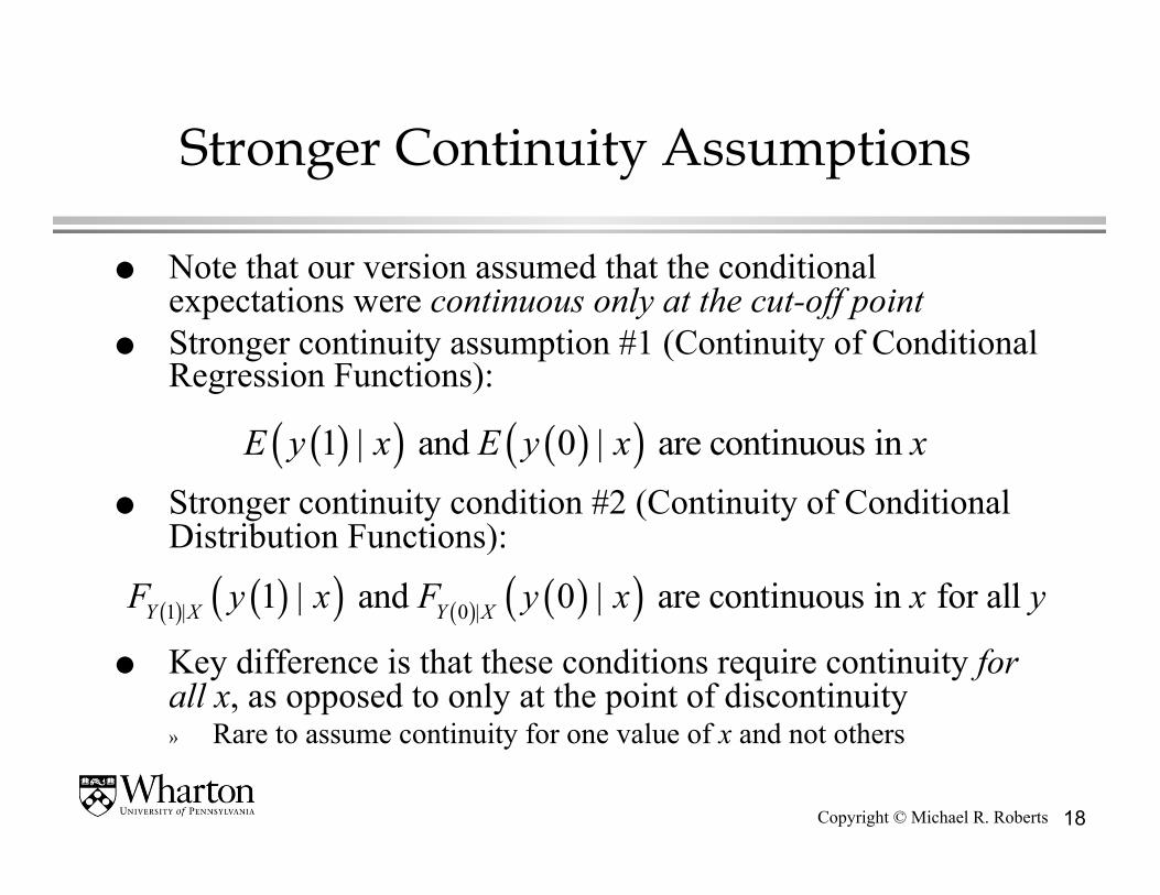
  Note that our version assumed that the conditional expectations were continuous only at the cut-off point

  Stronger continuity assumption #1 (Continuity of Conditional Regression Functions):

  Stronger continuity condition #2 (Continuity of Conditional Distribution Functions):

  Key difference is that these conditions require continuity for all x, as opposed to only at the point of discontinuity »  Rare to assume continuity for one value of x and not others

( )( ) ( )( )1 | and 0 | are continuous in E y x E y x x

( ) ( )( ) ( ) ( )( )1 | 0 |1 | and 0 | are continuous in for all Y X Y XF y x F y x x y


Implication of Local Continuity Assumption

  If density of x is positive in neighborhood containing x´,

  Comparing average outcomes just above and below the cut-off identifies the ATE for subjects close to the cut-off »  Equivalently, ATE is the difference of two regression functions at a

point »  Technical Point: Without parametric assumptions on regression

functions, consistency occurs at slower nonparametric rates (< N1/2).

( ) ( ) ( ) ( )

( ) ( )( )

' ' ' '

' '

lim | lim | lim | lim |

lim | lim |

|

i i i i ix x x x x x x x

i i ix x x x

i

E y x E y x E t x E u x

E t x E u x

E x

β

β

β

↓ ↑ ↓ ↓

↑ ↑

⎡ ⎤− = +⎣ ⎦⎡ ⎤− +⎣ ⎦

′=


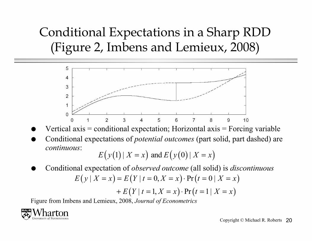
Conditional Expectations in a Sharp RDD (Figure 2, Imbens and Lemieux, 2008)

  Vertical axis = conditional expectation; Horizontal axis = Forcing variable   Conditional expectations of potential outcomes (part solid, part dashed) are

continuous:

  Conditional expectation of observed outcome (all solid) is discontinuous

( )( ) ( )( )1 | and 0 |E y X x E y X x= =

( ) ( ) ( )( ) ( )

| | 0, Pr 0 |

| 1, Pr 1 |

E y X x E Y t X x t X x

E Y t X x t X x

= = = = ⋅ = =

+ = = ⋅ = =Figure from Imbens and Lemieux, 2008, Journal of Econometrics


A Closer Look at the Local Continuity Assumption

  The continuity assumption formalizes the condition that subjects just above and below the cut-off are comparable – requiring them to have similar average potential outcomes when receiving treatment and when not

  Identification is achieved assuming only smoothness in expected potential outcomes at the discontinuity »  No parametric functional form restrictions

  Imposes a limitation on inference »  Without additional assumption (e.g., common effect βi = β), we only

learn about treatment effect for subpopulation close to cut-off »  With heterogeneous effects (βi ≠ β), local effect may be very different

from effect at values away from threshold. –  Doesn’t mean unimportant! Relevant issue may be choice of cut-off (e.g.,

expanding or limiting eligibility)


A Still Closer Look at the Local Continuity Assumption

  Note: even if treatment receipt is determined solely by cut-off, this is insufficient for identification

  Why? »  There may be coincidental functional discontinuities in the

yx relation »  E.g., Other programs that use assignment mechanism

based on the same assignment variable and cut-off   So, we need the continuity assumption as well

»  This assumption will also rule out certain behavior by potential treatment recipients and program administrators (more on this later)


Fuzzy RDD

  In a Fuzzy RDD treatment assignment depends on x in a stochastic manner but one where the propensity score function, Pr(ti = 1|x), has a known discontinuity at x´ »  Recall Sharp RDD where assignment occurs through a

known and measured deterministic decision rule:

  Instead of a 0-1 step function, treatment probability as a function of x can contain a jump at the cut-off that is less than one.

( ) ( )0 limPr 1 | limPr 1 | 1i ix x x xt x t x

′ ′↓ ↑< = − = <


Assignment to Treatment in a Fuzzy RDD (Figure 3, Imbens and Lemieux, 2008)

  Vertical axis = conditional probability of treatment Pr(ti = 1 | X = x); Horizontal axis = Forcing variable

  Cut-off for treatment assignment is x´ = 6   Probability of assignment jumps from 0.3 to 0.7 at cut-off

»  This is a key difference from the Sharp RDD, where the probability of assignment jumps from 0 to 1

Figure from Imbens and Lemieux, 2008, Journal of Econometrics


Fuzzy RDD Intuition

  Fuzzy RDD is akin to: »  mis-assignment relative to the cut-off value in a sharp RDD

–  Value of x near the cut-off appear in both treatment and control groups –  Mis-assignment can occur if, in addition to position relative to cut-off,

assignment is based on variables observed by administrator but not evaluator

»  random experiment with –  no-shows: treatment group members who do not receive treatment, and –  cross-overs: control group members who do receive treatment

  Practically speaking, imagine incentives to participate changing discontinuously at cut-off »  But not powerful enough to move all subjects from non-participant to

participant status


Fuzzy RDD Example

  Decision to offer a scholarship based on: »  Continuous measure of academic ability (e.g., GRE) exceeds given

cut-off, and »  Subjective information (e.g., recommendation letters) observed only

by the evaluator

  Does scholarship receipt impact academic achievement? »  Don’t compare recipients with non-recipients (even close to cut-off)

to estimate ATE likely differ along unobservables related to outcome (e.g., letters of rec)

»  But, could compare average outcomes of all subjects, irrespective of recipient status, just to the left and right of the cut-off…


Identifying the ATE in Fuzzy RDD

  Recall our regression:

which implies

  Recall local continuity assumption:

( ) ( ) ( ) ( )

( ) ( )


lim | lim |

i i i i i ix x x x x x x x

i ix x x x

E y x E y x E t x E t x

E u x E u x

β β′ ′ ′ ′↓ ↑ ↓ ↑

′ ′↓ ↑

⎡ ⎤− = −⎣ ⎦⎡ ⎤− +⎣ ⎦

i i i iy t uα β= + +

( )( ) ( )( )( ) ( )( )0 | and 1 | are continuous in at

or, | and | are continuous in at i i

E y x E y x x x

E x E u x x xβ

′

′


Identifying the ATE in Fuzzy RDD Case 1: Locally Constant Treatment Effect

  Locally constant (i.e., homogenous) treatment effect βi = β in a neighborhood around x´ »  Assuming local continuity as before yields

»  Common treatment effect is identified by

–  Denominator is change in Pr(treatment) at cut-off, and is always non-zero because of known discontinuity of E(t | x) at x´

–  For Sharp RDD, denominator just equaled 1

( ) ( ) ( ) ( )[ ]


1 0

i i i i i ix x x x x x x xE t x E t x E t x E t xβ β β

β β′ ′ ′ ′↓ ↑ ↓ ↑

⎡ ⎤ ⎡ ⎤− = −⎣ ⎦ ⎣ ⎦= − =

( ) ( )( ) ( )

lim | lim |

lim | lim |i ix x x x

i ix x x x

E y x E y x

E t x E t x′ ′↓ ↑

′ ′↓ ↑

−

−


Conditional Expectations in a Sharp RDD (Figure 4, Imbens and Lemieux, 2008)

  Vertical axis = conditional expectation; Horizontal axis = Forcing variable   Conditional expectations of potential outcomes (dashed) are continuous:

  Conditional expectation of observed outcome (all solid) is discontinuous ( )( ) ( )( )1 | and 0 |E y X x E y X x= =

( ) ( ) ( )( ) ( )

| | 0, Pr 0 |

| 1, Pr 1 |

E y X x E Y t X x t X x

E Y t X x t X x

= = = = ⋅ = =

+ = = ⋅ = =Figure from Imbens and Lemieux, 2008, Journal of Econometrics


Locally Constant Treatment Effect

  To nonparametrically identify a constant (across subjects) treatment effect at the cut-off, we need two assumptions

1.  Known discontinuity at the cut-off point

•  We are also implicitly assuming (i) existence of the limits, and (ii) a positive density for x in neighborhood containing x´

2.  Local continuity at the cut-off point

•  Since βi = β by assumption of constant treatment effects, we don’t need local continuity of β in x

( ) ( )lim | lim |i ix x x xE t x E t x

′ ′↓ ↑≠

( ) ( )lim | lim |i ix x x xE u x E u x

′ ′↓ ↑=


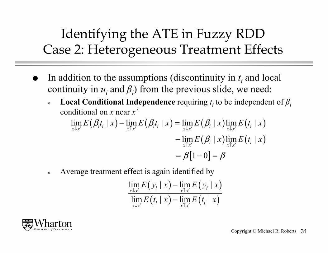
Identifying the ATE in Fuzzy RDD Case 2: Heterogeneous Treatment Effects

  In addition to the assumptions (discontinuity in ti and local continuity in ui and βi) from the previous slide, we need: »  Local Conditional Independence requiring ti to be independent of βi

conditional on x near x´

»  Average treatment effect is again identified by

( ) ( ) ( ) ( )( ) ( )

[ ]


lim | lim |

1 0

i i i i i ix x x x x x x x

i ix x x x

E t x E t x E x E t x

E x E t x

β β β

β

β β

′ ′ ′ ′↓ ↑ ↓ ↓

′ ′↑ ↑

− =

−

= − =

( ) ( )( ) ( )

lim | lim |


i ix x x x

E y x E y x

E t x E t x′ ′↓ ↑

′ ′↓ ↑

−

−


A Closer Look at the Local Conditional Independence Assumption

  If subjects self-select into treatment, or are selected for treatment on the basis of expected gain (i.e., as a function of the outcome variable) then conditional independence assumption may be violated

  What can we do when selection into the program is made on the basis of prospective gains? »  Employ an alternative set of assumptions to identify an

alternative treatment effect (Local Average Treatment Effect or LATE)


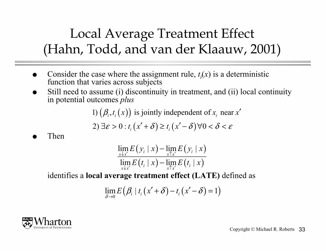
Local Average Treatment Effect (Hahn, Todd, and van der Klaauw, 2001)

  Consider the case where the assignment rule, ti(x) is a deterministic function that varies across subjects

  Still need to assume (i) discontinuity in treatment, and (ii) local continuity in potential outcomes plus

  Then

identifies a local average treatment effect (LATE) defined as

( )( )( ) ( )

1) , is jointly independent of near

2) 0 : 0i i i

i i

t x x x

t x t x

β

ε δ δ δ ε

′

′ ′∃ > + ≥ − ∀ < <

( ) ( )( ) ( )

lim | lim |


i ix x x x

E y x E y x

E t x E t x′ ′↓ ↑

′ ′↓ ↑

−

−

( ) ( )( )0

lim | 1i i iE t x t xδ

β δ δ→

′ ′+ − − =


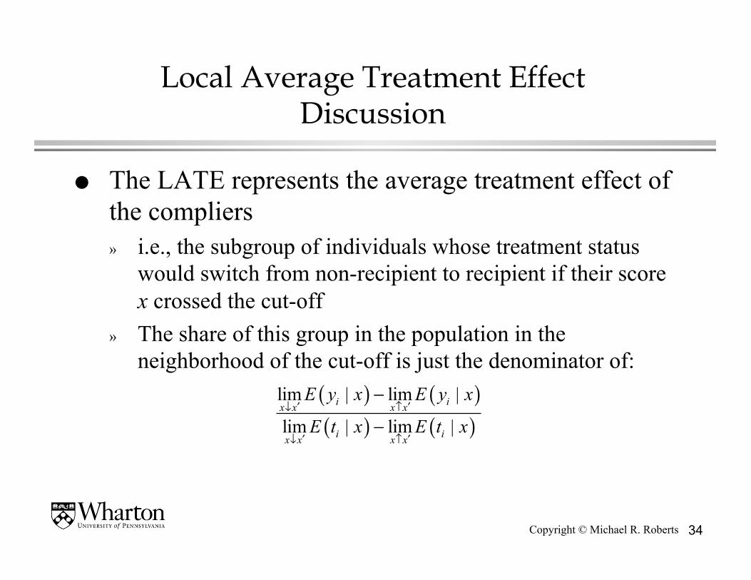
Local Average Treatment Effect Discussion

  The LATE represents the average treatment effect of the compliers »  i.e., the subgroup of individuals whose treatment status

would switch from non-recipient to recipient if their score x crossed the cut-off

»  The share of this group in the population in the neighborhood of the cut-off is just the denominator of:

( ) ( )( ) ( )

lim | lim |


i ix x x x

E y x E y x

E t x E t x′ ′↓ ↑

′ ′↓ ↑

−

−


Local Average Treatment Effect Illustration

  Scholarship awards based on score relative to cut-off and minority status: »  all minority students receive the scholarships, and »  only those non-minority students with high scores receive the

scholarships   If minority status is unobservable, scholarship assignment

rule corresponds to a Fuzzy RDD   LATE applies to subgroup of students with scores close to

cut-off for whom scholarship receipt depends on position of score relative to cutoff »  i.e., non-minority students.

  See van der Klaauw, 2008 and Chen and van der Klaauw, 2008 for examples.


Local Average Treatment Effect Another Illustration

  Imagine an eligibility rule dividing the population into eligibles and non-eligibles according to Sharp RDD and where eligibles self-select into treatment

  Battistin and Rettore, 2008 show that under local continuity assumption:

»  Implies that local continuity alone is sufficient for

to identify the average treatment effect on the treated, for those near the cut-off

( ) ( ) ( ) ( )[ ]

lim | lim | lim | 1, lim | 0

1 0

i i i i i i ix x x x x x x xE t x E t x E t x E t xβ β β

β β′ ′ ′ ′↓ ↑ ↓ ↓

⎡ ⎤ ⎡ ⎤− = = ⋅ −⎣ ⎦ ⎣ ⎦= ⋅ − =

( ) ( )( ) ( )

lim | lim |


i ix x x x

E y x E y x

E t x E t x′ ′↓ ↑

′ ′↓ ↑

−

−

( )| 1,i iE t x xβ ′= =


Internal and External Validity

  At best, Sharp and Fuzzy RDD estimate the average effect of the sub-population with x close to x´ »  Fuzzy RDD restricts this subpopulation even further to

that of the compliers with x close to x´   Only with strong assumptions (e.g., homogenous

treatment effects) can we estimate the overall average treatment effect

  So, RDD have strong internal validity but weak external validity


Implementation Graphical Analysis

  A plot of the outcome variable y against the forcing variable x should reveal a clear discontinuity at the cut-off »  Think of the solid line in the earlier figures »  May want to plot residuals from regression of outcome on covariates

(e.g., fixed effects, characteristics, etc.) if heterogeneity is concern   For example,

Figures from Angrist and Pischke, 2009, Mostly Harmless Econometrics


Discontinuity vs. Nonlinearity

  Take care not to confuse a nonlinear relation with a discontinuity

  Plot estimated polynomial or nonparametric regression to help guard against this

Figure from Angrist and Pischke, 2009, Mostly Harmless Econometrics


Histogram of Average Outcomes against Forcing Variable

  Construct equal-sized non-overlapping bins of the forcing variable such that no bin includes points to both the left and right of the cut-off

  For each bin, compute the average outcome so see if there is a discontinuity at the cut-off

  Recipe: 1.  Choose a bin width h 2.  Choose a # of bins to the left (K0) and right (K1) of the cut-off 3.  Construct the bins, (bk,bk+1], for k=1,…,K=K0+K1: bk = x – (K0 – k + 1) · h 4.  Calculate the # of observations in each bin:

5.  Compute the average outcome in each bin:

6.  Plot each average against the corresponding bin mid point

( )11

n

k k i ki

N I b x b +=

= < ≤∑

( )11

1 n

k i k i kik

Y Y I b x bN +

=

= ⋅ < ≤∑


Plots of Outcome against Forcing Variable – Other Things to Look Out For

  Check to make sure that there aren’t comparable jumps in the conditional expectation at points other than the cutoff »  The existence of such jumps doesn’t invalidate the RDD,

but does require an explanation »  Concern is that the relation is fundamentally discontinuous

and jump at cut-off is contaminated by other factors.


Plots of Covariate Outcomes against Forcing Variable

  Ideally, subjects on both sides of the cut-off are “similar” in terms of average observed and unobserved characteristics

  Repeat the histogram exercise for covariates: Do we see a similar discontinuity? »  If so, could be a threat to identification…must explain the

discontinuity   Alternative test is to run the RDD estimation using the

covariates as the outcome variable »  Relation between observable covariates and treatment should ideally

be smooth »  Alternatively, we can condition on covariates but one should be

suspicious given underlying rationale for RD (subjects are similar close to cut-off)


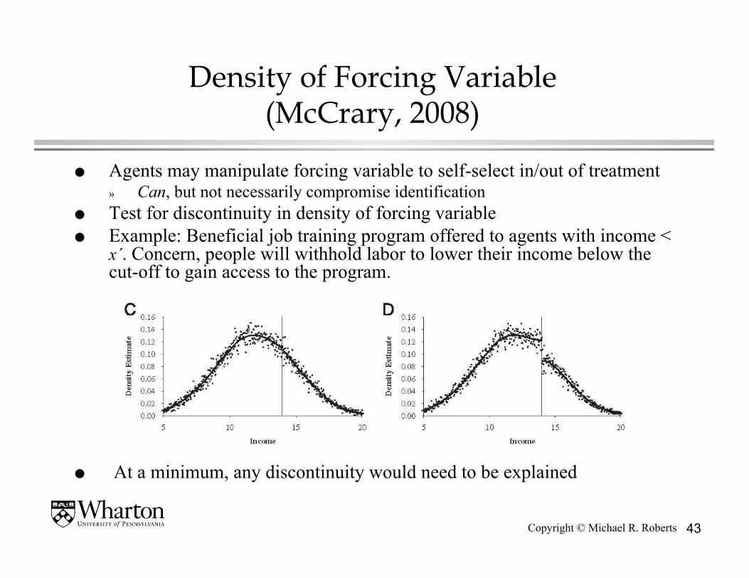
Density of Forcing Variable (McCrary, 2008)

  Agents may manipulate forcing variable to self-select in/out of treatment »  Can, but not necessarily compromise identification

  Test for discontinuity in density of forcing variable   Example: Beneficial job training program offered to agents with income <

x´. Concern, people will withhold labor to lower their income below the cut-off to gain access to the program.

  At a minimum, any discontinuity would need to be explained


Estimation

  How do we estimate the treatment effect? »  Strictly speaking, we need to estimate boundary points of conditional

expectations. Recall ATE, under appropriate assumptions, in –  Sharp RDD:

–  Fuzzy RDD:

  With enough observations, we could focus on agents in a very small interval around the cut-off and compare average outcomes for agents just to the left and right of the cut-off »  Increasing the interval, increases the bias

( ) ( )lim | lim |i ix x x xE y x E y x

′ ′↓ ↑−

( ) ( )( ) ( )

lim | lim |

lim | lim |x x x x

x x x x

E y x E y x

E t x E t x′ ′↓ ↑

′ ′↓ ↓

−

−


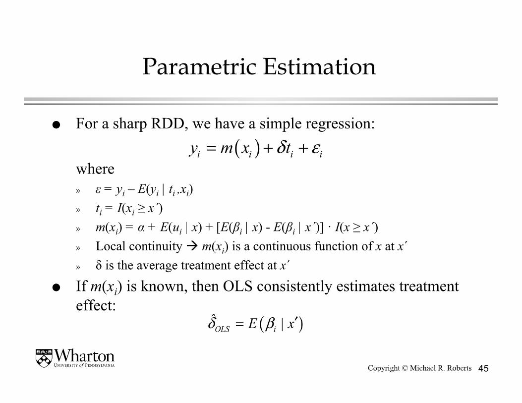
Parametric Estimation

  For a sharp RDD, we have a simple regression:

where »  ε = yi – E(yi | ti ,xi) »  ti = I(xi ≥ x´) »  m(xi) = α + E(ui | x) + [E(βi | x) - E(βi | x´)] · I(x ≥ x´) »  Local continuity m(xi) is a continuous function of x at x´ »  δ is the average treatment effect at x´

  If m(xi) is known, then OLS consistently estimates treatment effect:

( )i i i iy m x tδ ε= + +

( )ˆ |OLS iE xδ β ′=


What is m(xi)?

  Don’t know so we “guess” with flexible functional forms »  Global polynomials »  Splines (e.g., piecewise polynomials) where m(x) is specified as a

different polynomial function of x on either side of the cut-off –  E.g., Trochim, 1984; van der Klaauw, 2002; McCrary, 2008

»  Linear specifications not robust   Aside: m(x), which corrects for selection bias, is known as a

control function (Heckman and Robb, 1985) which »  allows us to expand the sample beyond the subset of observations

close to cut-off, but »  requires a large sample because of collinearity between terms in m(x)

and t in the regression equation –  This reduces independent variation in status across obs and inflates SEs –  RDD requires 2.75 – 4 times sample size as random experiment

(Goldberger, 1972; Bloom et al., 2005)


Parametric estimation in Fuzzy RDD

  What is there is mis-assignment relative to the cut-off? »  Including m(x) in regression is insufficient for to avoid

biases due to group non-equivalence –  Exception: random mis-assignment (Cain, 1975)

»  Insufficiency remains in other Fuzzy RDDs –  δ is estimated with bias, which depends on cov(t , ε | x), which can

be >< 0


Parametric estimation in Fuzzy RDD Solution to Selection Problem

  Control function-augmented outcome equation where ti is replaced by estimated propensity score, E(ti | x) »  Assuming local independence of ti and βi conditional on x then

»  in a neighborhood of x´,where –  ε = yi – E(yi | xi) –  m(x) = α + E(ui | x) + [E(βi | x) – E(βi | x´) · E(t | x)

»  Local continuity m(x) is continuous at x´ , and E(ti | xi) is discontinuous at x´ δ measures

which is the average local treatment effect E(βi | x´) »  δ is a LATE if we replace local independence with local monotonicity

( ) ( )|i i i i iy m x E t xδ ε= + +

( ) ( )( ) ( )

lim | lim |


i ix x x x

E y x E y x

E t x E t x′ ′↓ ↑

′ ′↓ ↑

−

−


Estimation Implementation: Two-Stage Procedure (van der Klaauw, 2002)

  Stage 1: Estimate treatment or selection rule in the fuzzy RDD as:

where f(·) is a function of x continuous at x´. »  γ estimates the discontinuity in the propensity score function at x´

  Stage 2: Estimate control-function-augmented outcome equation replacing ti with first-stage estimate of E(ti | x) = Pr(ti = 1 | xi).

»  If f and m are correctly specified, then consistent estimate of δ »  If f and m have same functional form, then this is 2SLS with I(xi ≥ x´)

and m(x) as the instruments. (Exclusion restriction on I(xi ≥ x´).)

( ) ( ) ( )|i i i i i i it E t x f x I x xν γ ν′= + = + ≥ +

( ) ( )|i i i i iy m x E t xδ ε= + +


Specification Concerns

  For parametric estimation: »  Valid inference requires correct specification of control

function m(x) and of f(x). »  Identification rests on local continuity, but parametric

estimation imposes global continuity and often global differentiability (except at discontinuity point) of conditional expectation functions –  This lets us use points far from the cut-off but the choice of

functional form and order of the polynomial in polynomial specifications is delicate


Semi-parametric Estimation

  Reduce potential for mis-specification bias by continuing to assume global continuity and differentiability, but estimate m and f semi-parametrically.

  Example »  van der Klaauw, 2002: power series approximation

–  larger SEs because chosen polynomial is an approximation »  HTV (2001): kernel methods

–  Conditional expectations estimated using Nadaraya-Watson estimators –  While consistent, poor asymptotic bias behavior common to non-

parametric estimators at boundary points »  Porter (2003) (and HTV (2001)) (2001): local polynomial regression

–  optimal rate of convergence »  Porter (2003) partially linear model

–  Uses data from both sides of cut-off biases cancel out –  Poor performance with heterogeneous effects


Sensitivity Analysis 1 (a.k.a., The Laundry List of Robustness Tests)

  Check sensitivity of estimates to alternative specifications »  e.g., add higher order polynomials, vary bandwidth, etc.

  Restrict attention to subsample of observations close to the cut-off »  You can be more restrictive with the control function here

since the small distance will act as an instrument »  This reduces bias but also reduces efficiency



  Can subjects behavior invalidate the local continuity assumption? »  Can they exercise control over their values of the assignment variable? »  Can administrators strategically choose what assignment variable to

use or which cut-off point to pick? »  Either can invalidate the comparability of subjects near the threshold

because of sorting of agents around the cut-off, where those below may differ on average form those just above

  Continuity violated in the presence of other programs that use a discontinuous assignment rule with the exact same assignment variable and cut-off



  Even if agents or administrators (or both) exercise some control over the forcing variable or cut-off position, continuity assumptions may not be violated »  Lee (2008) shows that in Sharp RDD, as long as agents do not have

perfect control, continuity will be satisfied. –  i.e., there must be some independent random chance element –  Implies local conditional independence assumption will be satisfied –  Manipulation will identify a weighted ATE

  Sorting undermines the causal interpretation of RDD only if sorting is perfect »  Perhaps a break/discontinuity in the forcing variable (McCrary (2008))



  Test for comparability of agents around the cut-off »  Visual test of covariates discussed earlier »  Repeat RDD using the characteristics as outcome variables (van der

Klaauw (2008)) »  Finding a discontinuity does not necessarily invalidate the RDD »  Incorporate covariates, z, in the RDD, as additional controls

–  This should only impact stat significance, not magnitude of treatment effect

–  Alternatively, regress the outcome variable on a vector of controls and use the residuals in the RDD, instead of the outcome itself

  This only addresses observables, not unobservables



  Falsification tests »  Test whether the treatment effect is zero when it should be

–  e.g., at points away from the discontinuity

»  Maybe data exists in a period where there was no program »  Test whether the actual cut-off fits the data better than

near-by cut-offs –  A spike in the log-likelihood at the actual relative to alternative

cut-off values can allay concerns that the found local relationship was spurious


Multiple Dose Levels or Cut-Off

  RDD does not have to be restricted to a binary effect »  Angrist and Lavy (1999) – jumps at multiples of max class size »  van der Klaauw (2002) – jumps at multiple score levels

  Imagine multiple dose levels or multiple cut-offs for t »  Regression equation

describes average potential outcomes across individuals under alternative treatment dose assignments

»  Under Sharp RDD, impact defined at a discontinuity point

is the average impact of a change in treatment does equal to the jump at the discontinuity point for agents near the cut-off

i i i iy t uα β= + +

( ) ( )( ) ( )

lim | lim |


i ix x x x

E y x E y x

E t x E t x′ ′↓ ↑

′ ′↓ ↑

−

−


Summary

  Sharp RDD »  Graph data: Average outcomes by forcing variable (discontinuity at

cut-off?) »  Estimate treatment effect: Use several methods for robustness »  Perform sensitivity analysis: Not just econometrics, think about

economics and potential concerns   Fuzzy RDD

»  Graph data: Average outcomes by forcing variable and Pr(treatment) »  Estimate treatment effect: Use 2SLS and other methods for robustness »  Perform sensitivity analysis: Not just econometrics, think about

economics and potential concerns   Enjoy


References I

  Angrist, Joshua, and Victor Lavy, 1999, Using Maimonides rule to estimate the effect of class size on scholastic achievement, Quarterly Journal of Economics 114, 533-575

  Battistin, E., and E. Rettore, 2008, Ineligibles and eligible non-participants as a double comparison group in regression discontinuity designs, Journal of Econometrics 142, 715-730

  Bloom, H. S., J. Kemple, B. Gamse, and R. Jacob, 2005, Using regression discontinuity analysis to measure the impacts of reading first

  Chen, S., and Wilbert van der Klaauw, 2008, The work disincentive effects of the disability insurance program in the 1990s, Journal of Econometrics 142, 757-784

  Goldberger, A. S., 1972, Selection bias in evaluating treatment effects: Some formal illustrations, Discussion Paper 123-172, Madison, IRP

  Heckman, James J. and R. Robb, 1985, Alternative methods for evaluating the impact of interventions, in Heckman J. and B. Singer (eds.) Longitudinal Analysis of Labor Market Data, Cambridge University Press, New York


References II

  Hahn, Jinyong, Petra Todd, and Wilbert van der Klaauw, 2001, Identification and estimation of treatment effects with a regression-discontinuity design, Econometrica 69, 201-209

  Imbens, Guido, and Thomas Lemieux, 2008, Regression discontinuity designs: A guide to practice, Journal of Econometrics 142, 615-635

  McCrary, Justin, 2008, Testing for manipulation of the running variable in the regression discontinuity design, Journal of Econometrics 142, 698-714

  Trochim, W. K., 1984, Research design for program evaluation: The regression-discontinuity approach, Sage, Beverly Hills

  van der Klaauw, Wilbert, 2002, Estimating the effect of financial aid offers on college enrollment: A regression-discontinuity approach, International Economic Review 43, 1249-1287

  van der Klaauw, Wilbert, 2008, Regression-discontinuity analysis: A survey of recent developments in economics, Labour, 220-245

empirical methods - wharton...

Documents