Employment Hysteresis from the Great Recession∗

Danny YaganUC Berkeley and NBER

August 2018

Abstract

This paper uses U.S. local areas as a laboratory to test for long-term impacts ofthe Great Recession. In administrative longitudinal data, I estimate that exposure toa 1-percentage-point-larger 2007-2009 local unemployment shock reduced 2015 working-age employment rates by over 0.3 percentage points. Rescaled, this long-term recessionimpact accounts for over half of the 2007-2015 U.S. age-adjusted employment decline.Impacts were larger among older and lower-earning individuals and typically involveda layoff. However, recession exposure reduced 2015 employment even in a mass-layoffssample. Disability benefits replaced less than 6% of lost 2015 earnings while out-migrationyielded no replacement. These findings reveal that the Great Recession imposed long-termemployment and income losses even after unemployment rates signaled recovery.

∗Email: yagan@berkeley.edu. I thank Patrick Kline, David Autor, David Card, Raj Chetty, Hilary Hoynes,Erik Hurst, Lawrence Katz, Matthew Notowidigdo, Evan K. Rose, Jesse Rothstein, Emmanuel Saez, AntoinetteSchoar, Lawrence Summers, Till Von Wachter, Owen Zidar, Eric Zwick, seminar participants, and anonymousreferees for helpful comments. Rose, Sam Karlin, and Carl McPherson provided outstanding research assistance.I acknowledge financial support from The Laura and John Arnold Foundation and the Berkeley Institute forResearch on Labor and Employment. This work is a component of a larger project examining the effects oftax expenditures on the budget deficit and economic activity; all results based on tax data in this paper areconstructed using statistics in the updated SOI Working Paper The Home Mortgage Interest Deduction andMigratory Insurance over the Great Recession, approved under IRS contract TIRNO-12-P-00374 and presentedat the National Tax Association. The opinions expressed in this paper are those of the author alone and do notnecessarily reflect the views of the Internal Revenue Service or the U.S. Treasury Department.

1 Introduction

The U.S. unemployment rate spiked from 5.0% to 10.0% over the course of the Great Reces-

sion and then returned to 5.0% in 2015. However, the U.S. employment rate (employment-

population ratio) did not exhibit similar recovery. Figure 1A shows that the employment rate

declined 3.6 percentage points between 2007 and 2015, as millions of adults exited the labor

force.1 Population aging explains a minority of the employment rate decline: weighting 2015

ages by the 2007 age distribution reduces the decline to 2.0 percentage points, and the unad-

justed age-25-54 employment rate declined 2.6 percentage points. The decline was concentrated

among the low-skilled (Charles, Hurst and Notowidigdo 2016). The decline’s persistence con-

trasts with employment rate recovery after earlier recessions—leading history-based analyses

like Fernald, Hall, Stock and Watson (2017) to doubt the possibility of employment hystere-

sis: the Great Recession having depressed long-term employment despite the unemployment

recovery.

This paper tests whether the Great Recession and its underlying sources caused part of

the 2007-2015 age-adjusted decline in U.S. employment, or whether that decline would have

prevailed even in the absence of the Great Recession. It is typically difficult to test for long-term

employment impacts of recessions, for the simple reason that recession-independent (“secular”)

forces may also affect employment over long horizons (Ramey 2012). For example, the U.S.

employment rate rose by two percentage points from the start of the 1981-1982 recession to the

late 1980s, as women continued to enter the labor force. In the context of the Great Recession,

secular nationwide skill-biased shocks like technical or trade changes could have caused the

entire 2007-2015 employment decline, rather than the recession.

I attempt to overcome this challenge by leveraging spatial variation in Great Recession

severity along with data that minimize selection threats. All U.S. local areas by definition

experienced the same secular nationwide shocks, but some local areas experienced more severe

Great Recession shocks than other local areas. For example: Phoenix, Arizona—America’s sixth

1Variable definitions are standard and pertain to the age-16-and-over civilian noninstitutional population.

1

largest city—experienced a relatively large unemployment spike during the Great Recession

while San Antonio, Texas—America’s seventh largest city—did not. A cross-area research

design has the potential to distinguish recession impacts from secular nationwide shock impacts.

In the first part of the paper, I show using public state-year aggregates that a cross-area

research design is indeed fertile ground for studying the labor market consequences of the

Great Recession. Defining state-level shocks as 2007-2009 employment growth forecast errors

in an autoregressive system (Blanchard and Katz 1992), I find that 2015 employment rates

remained low in the U.S. states that experienced relatively severe Great Recession shocks—even

though between-state differences in unemployment rates had returned to normal (and despite

normal between-state population reallocation). Hence, the cross-area patterns of employment,

unemployment, and labor force participation closely mirrored the aggregate cross-time patterns

of Figure 1A. The persistent cross-area employment rate difference departs from the Blanchard-

Katz finding of rapid regional convergence.

The state-year evidence does not imply employment hysteresis from the Great Recession,

because of two potential forms of cross-area composition bias: post-2007 sorting on labor supply

and pre-2007 sorting on human capital. First, severe Great Recession local shocks caused

long-term declines in local costs of living (Beraja, Hurst and Ospina 2016) which may have

disproportionately attracted or retained those secularly out of the workforce like the disabled

and retired (Notowidigdo 2011).2 Even without such post-2007 sorting on labor supply, severe

Great Recession local shocks may have happened to hit areas with particularly large pre-existing

concentrations of individuals affected by secular nationwide shocks. For example, the Great

Recession disproportionately struck local areas that had experienced housing booms (Mian

and Sufi 2014) attracting low- and middle-skill construction labor, and low- and middle-skill

laborers have been relatively adversely affected by secular nationwide shocks in recent decades

(e.g. Katz and Murphy 1992).3 Under either type of cross-area sorting, severe Great Recession

2For example: “Warren Buffett’s Advice to a Boomer: Buy Your Sunbelt Retirement Home Now”(Forbes 2012 http://www.forbes.com/sites/janetnovack/2012/01/27/warren-buffetts-advice-to-a-boomer-buy-your-sunbelt-retirement-home-now/).

3For example: “You can’t change the carpenter into a nurse easily...monetary policy can’t retrain people”(Charles Plosser, http://www.wsj.com/articles/SB10001424052748704709304576124132413782592).

2

local shocks may not have caused local residents’ 2015 nonemployment.

I therefore turn for the second part of the paper to longitudinal linked-employer-employee

data in order to control for prominent dimensions of cross-area sorting. The longitudinal com-

ponent allows one to measure individuals’ employment over time regardless of whether and

where in the United States they migrated—directly controlling for post-2007 sorting on labor

supply. The linked-employer-employee component allows one to control for fine interactions of

age, 2006 earnings, and 2006 industry—proxies for pre-2007 human capital.

Specifically, I draw a 2% random sample of individuals from de-identified federal income

tax records spanning 1999-2015. The main outcome of interest is employment at any point

in 2015, equal to an indicator for whether the individual had any W-2 earnings or any 1099-

MISC independent contractor earnings in 2015. The main sample restricts to those aged 30-49

(“working age”) in 2007 in order to confine the 1999-2015 employment analysis to those between

typical schooling and retirement age, and it restricts to American citizens in order to minimize

unobserved employment in foreign countries. The analysis allows for within-state variation

by using the local area concept of the Commuting Zone (CZ): 722 county groupings that

approximate local labor markets and are similar to metropolitan statistical areas but span the

entire continental United States. I use the universe of information returns to assign individuals

to their January 2007 CZ. Each individual’s Great Recession local shock equals the percentage

point change in her 2007 CZ’s unemployment rate between 2007 and 2009 as recorded in the

Bureau of Labor Statistics Local Area Unemployment Statistics. I obtain 2006 four-digit NAICS

industry for half of 2006 W-2 earners by linking W-2s to employers’ tax returns.

I find that conditional on 2006 age-earnings-industry fixed effects, a 1-percentage-point-

higher Great Recession local shock caused the average working-age American to be 0.39 per-

centage points less likely to be employed in 2015. The estimate is very statistically significant,

approximately linear in shock intensity, robust across numerous specifications, and large: those

living in 2007 in largest-shock-quintile CZs were 1.7 percentage points less likely to be employed

in 2015 than initially similar individuals living in 2007 in smallest-shock-quintile CZs. Placebo

tests indicate no relative downward employment trend in severely shocked areas before the

3

recession, corroborating identification. Controlling for 2015 local unemployment rates suggests

that the incremental 2015 nonemployment took the form of labor force exit rather than long-

term unemployment. I similarly find impacts on 2015 wage and contractor earnings: −3.6%

(−$997) of the individual’s pre-period earnings for every 1-percentage-point-higher shock.

One could be concerned that the foregoing within-industry analysis fails to sufficiently con-

trol for pre-2007 sorting on human capital, as jobs and therefore skill types in some industries

are geographically differentiated. Thus as a novel robustness check, I approximate a within-job

analysis using a sample of 2006 workers at retail chain firms like Walmart and Safeway that

employ workers with similar skills to perform similar tasks at similar salaries in many different

local areas. Adding firm fixed effects in the retail sample attenuates the retail-sample employ-

ment effect by 0.05 percentage points, or one half of one standard error, to −0.36 percentage

points.

Certain comparisons suggest that the true average employment impact could be closer to

−0.30 percentage points per percentage-point unemployment rate shock. Naive extrapolation

of those −0.30-for-1 and −0.39-for-1 magnitudes would explain 58-76% of the U.S. 2007-2015

working-age annual employment rate decline as a long-term impact of the Great Recession. The

actual implied aggregate impact depends on general equilibrium amplification or dampening.

The recession’s impacts were highly uneven within local areas. The employment and earn-

ings impacts were most negative for older individuals and those with low 2006 earnings. The

latter pattern indicates that the Great Recession induced a long-term increase in employment

and earnings inequality across skill levels, not merely within skill levels across space. Impacts

do not appear smaller among mobile subgroups like renters or the childless.

Adjustment via migration and social insurance appears highly incomplete in replacing lost

income. I find no statistically significant impact of Great Recession local shocks on out-

migration from one’s 2007 CZ, and earnings in other CZs did not replace any lost 2015 earnings

relative to those exposed to smaller Great Recession local shocks. Great Recession local shocks

caused significantly higher unemployment insurance (UI) benefits 2008-2010 before UI bene-

fits expired and insignificantly higher Social Security Disability Insurance (SSDI) benefits in

4

all years. I estimate that 2015 SSDI replaced 2% of lost 2015 earnings, or up to 6% at the

95%-confidence upper bound.

Finally, I find that most of the 2015 incrementally nonemployed in severely shocked areas

had been laid off at some point 2007-2014 and were entirely nonemployed 2013-2015. However,

higher layoff rates do not appear to explain the results, as the impacts hold within laid-off

individuals. In particular, I find equally large impacts when comparing workers who were each

displaced in a 2008-2009 mass layoff. Hence, interactions with area-level economic conditions

appear key to any full explanation of the long-term impacts—such as human capital decay

during extended nonemployment, or persistently low local labor demand.

The paper’s findings constitute evidence of employment hysteresis from the Great Recession

(cf. Fernald, Hall, Stock and Watson 2017) and add to a large literature on the incidence of labor

market shocks. Earlier work had found long-term impacts on individuals’ earnings (Topel 1990,

Jacobson, LaLonde and Sullivan 1993, Neal 1995, Kahn 2010, Davis and Von Wachter 2011) and

sometimes on local areas’ employment rates (Blanchard and Katz 1992 vs. Black, Daniel and

Sanders 2002 and Autor and Duggan 2003) and individuals’ employment rates (Ruhm 1991,

Walker 2013 vs. Autor, Dorn, Hanson and Song 2014, Jarosch 2015). I provide evidence of

long-term impacts of Great Recession local shocks on individuals’ employment rates, likely via

labor force exit. This evidence reinforces the view of Autor and Duggan and a large literature

dating back at least to Bowen and Finegan (1969) and Phelps (1972) that transitory adverse

aggregate shocks can have persistent negative employment impacts even after unemployment

recovers.

The rest of the paper is organized as follows. Section 2 uses state-year data to show that

cross-area employment patterns mirrored aggregate cross-time employment patterns 2007-2015.

Section 3 details the empirical design and longitudinal linked-employer-employee data. Section

4 estimates overall impacts. Section 5 estimates impact heterogeneity. Section 6 investigates

adjustment margins. Section 7 documents layoff and nonemployment trajectories. Section 8

discusses candidate mechanisms. Section 9 concludes.

5

2 Local Labor Markets Mirrored the Aggregate

This paper uses cross-area variation in Great Recession severity to test whether the recession

and its underlying sources caused part of the 2007-2015 decline in the U.S. employment rate

displayed in Figure 1A. I begin by testing whether Figure 1A’s aggregate cross-time employ-

ment patterns have been mirrored across U.S. local areas: did the local areas that experienced

severe Great Recession shocks also experience persistent declines in employment and partici-

pation rates but not unemployment rates, relative to mildly shocked areas? If so, then local

labor markets may indeed serve as a fruitful laboratory for understanding sources of aggregate

employment patterns.

A large literature has studied local labor market dynamics after local employment shocks.

The canonical analysis of Blanchard and Katz (1992) found in state-year data 1976-1990 that,

when a state experiences an adverse employment shock, its population falls relative to trend

but its unemployment, participation, and employment rates return to parity with other states

in five-to-six years. That is, local shocks leave local areas smaller but no less employed. This

conclusion has been replicated in European data (Decressin and Fatas 1995) and in a longer

U.S. state-year time series (Dao, Furceri and Loungani 2017). However, other papers have found

long-term participation and employment impacts of local shocks: Black, Daniel and Sanders

(2002), Autor and Duggan (2003), and Autor, Dorn and Hanson (2013) found long-term impacts

of specific types of U.S. local shocks on local disability insurance enrollment, participation,

and/or employment rates. Hence, the existing literature presents a mixed picture.

This section documents local labor market dynamics after Great Recession local employment

shocks, with greater detail presented in Online Appendices B and C. For comparability to the

broadest line of previous work, I conduct this analysis at the state level and categorize states

into severely shocked states and mildly shocked states using unforecasted state-level changes in

2007-2009 employment, derived from the autoregressive system of Blanchard and Katz (1992).

I estimate Blanchard and Katz’s log-linear autoregressive system in state employment growth,

state unemployment rates, and state participation rates in LAUS data 1976-2007. The LAUS

6

data are the annual Bureau of Labor Statistics Local Area Unemployment Statistics series of

employment, population, unemployment, and labor force participation counts 1976-2015 for 51

states (the 50 states plus the District of Columbia). Annual counts are calendar-year averages

across months. I then compute 2008 and 2009 employment growth forecast errors for each

state—equal to each state’s actual log employment growth minus the system’s prediction for

that state—and sum the two to obtain each state’s 2007-2009 employment shock. Roughly

speaking, each state’s shock equals the state’s 2007-2009 log employment change minus the

state’s long-run trend. Then for expositional simplicity, I group the 26 states with the most

negative shocks (e.g. Arizona) into a severely shocked category and the remaining states (e.g.

Texas) into a mildly shocked category.

Figure 1B displays the 2003-2015 time series of unemployment, participation, and employ-

ment rate differences between severely shocked states and mildly shocked states. For each

outcome and year, the graph plots the unweighted mean among severely shocked states, mi-

nus the unweighted mean among mildly shocked states (the graph looks nearly identical when

weighting by population). Within each series, I subtract the mean pre-2008 severe-minus-mild

difference from each data point, so each plotted series has a mean of zero before 2008.

The figure shows that the unemployment rate in severely shocked states relative to mildly

shocked states spiked in 2008, peaked in 2009-2010, and returned by 2015 to its mean pre-

recession severe-mild difference. Yet the 2015 employment and participation rates in severely

shocked states remained 1.74 percentage points below the corresponding rates in mildly shocked

states, relative to the mean pre-recession severe-mild differences. The implied 2015 cross-area

employment gap is large: 2.01 million fewer adults were employed in severely shocked states than

in mildly shocked states, relative to full recovery to the pre-recession severe-mild employment

rate difference.

Hence, the cross-area (severe-minus-mild) patterns of unemployment, participation, and em-

ployment of Figure 1B do indeed broadly mirror the aggregate cross-time (current-minus-2007)

patterns of Figure 1A. Moreover in the same sense that the aggregate employment aftermath of

the Great Recession appears to contrast with the aftermath of the early-1980s and early-1990s

7

recessions, so too does the cross-area aftermath of the Great Recession appear to contrast with

the cross-area aftermath of those earlier recessions. Figure 2A repeats the employment rate

series of Figure 1B for the aftermath of the 1980s and 1990s recessions, treating the early-1980s

recessions as a single recession. The figure shows that cross-state employment rates fully con-

verged four years after the early-1990s recession and had converged by 1.65 percentage points

(78% of the t=0 divergence) six years after the early-1980s recession. Six-year convergence after

the Great Recession was smaller in both absolute terms (0.85 percentage points) and relative

to the t=0 divergence (33%).

Blanchard and Katz suggest that the historical convergence mechanism is rapid population

reallocation: a −1% state population change relative to trend follows every −1% employment

shock within five-to-six years.4 Therefore a natural possible explanation for local employment

rate persistence after the Great Recession is that population reallocation has slowed. Figure

2B investigates this possibility by plotting de-trended 2007-2014 population changes—equal to

each state’s 2007-2014 percent change in population minus the 2000-2007 percent change in

the state’s population—versus the state’s 2007-2009 employment shock. The graph shows that

population reallocation after the Great Recession was similar to the historical benchmark: each

−1% 2007-2009 employment shock was on average accompanied by a −1.016% (robust standard

error 0.260) de-trended population change.5 Figure 2C shows the same conclusion when using

the original Blanchard-Katz time range—1976-1990, well before the recent housing boom—to

estimate state-specific population trends in the Blanchard-Katz system. Population in severely

shocked states fell 2007-2015 relative to trend and relative to mildly shocked states as much as

in the Blanchard-Katz benchmark.

4The unit elastic population response holds when re-estimating the Blanchard and Katz system on updateddata 1976-2015. The suggested causal chain is: a state (e.g. Michigan) experiences a one-time random-walkcontraction in global consumer demand for its locally produced traded good (e.g. cars), which induces a locallabor demand contraction and wage decline, which in turn induces a local labor supply (population) contraction,which then restores the original local wage and employment rate.

5When not de-trending, state population changes were largely uncorrelated with 2007-2009 employmentshocks, also shown in Mian and Sufi (2014) for the 2007-2009 period only. Blanchard and Katz find adjustmentvia population changes relative to trend. Gross (out-)migration rates have declined modestly since 1980 (Molloy,Smith and Wozniak 2011), but gross flows are still an order of magnitude larger than the net flows (populationreallocations) predicted by history in response to 2007-2009 shocks.

8

To sum up, this section has found that aggregate 2007-2015 cross-time unemployment,

participation, and employment rate patterns have been mirrored in cross-area unemployment,

participation, and employment rate patterns over the same time period. Participation and em-

ployment rates remained persistently low in the U.S. states that experienced relatively severe

employment shocks 2007-2009, even though unemployment rates converged across space. Re-

duced population reallocation does not explain the local persistence. The cross-area aftermath

of the Great Recession departs from the broad historical findings of Blanchard and Katz (1992),

but they accord with findings of Black, Daniel and Sanders (2002), Autor and Duggan (2003),

and Autor, Dorn and Hanson (2013) from specific contexts. I now turn to identifying whether

Great Recession local shocks caused individuals to have lower 2015 employment.

3 Isolating Impacts of Great Recession Local Shocks

The previous section showed that local labor markets were microcosms of aggregate employment

patterns 2007-2015: 2015 employment rates remained unusually low in U.S. local areas that

experienced an especially severe 2007-2009 employment shock. However, that cross-sectional

fact does not imply that individuals were nonemployed in 2015 because of where they were

living during the Great Recession, in light of two selection threats. First, the disabled, retirees,

and others secularly out of the labor force may have disproportionately stayed in or moved to

severely shocked areas in order to enjoy low living costs while foregoing employment. Even

without selective migration on post-2007 labor supply, severely shocked areas may have been

disproportionately populated before the recession by individuals who subsequently suffered large

nationwide contractions for their skill types, like construction workers or routine laborers, that

would have occurred even in the absence of the recession. Under either selection threat, the

2015 residents of severely shocked areas might be nonemployed now regardless of geography.

This section specifies my empirical strategy for using longitudinal linked-employer-employee

data to isolate causal effects of Great Recession local shocks on individuals’ 2015 employment.

2015 is the most recent year of data available. Additional details are listed in Online Appendices

9

D and E, including design foundations in potential outcomes.

3.1 Empirical Design

I adopt an empirical design that closely follows earlier work using longitudinal individual-

level data to estimate long-term impacts of labor market shocks (e.g. Jacobson, LaLonde and

Sullivan 1993, Davis and Von Wachter 2011, Autor, Dorn, Hanson and Song 2014). I estimate

regressions of the form:

yi2015 = βSHOCKc(i2007) + θg(i2006) + εi2015 (3.1)

where y denotes an employment or related outcome; i denotes an individual; SHOCKc(i2007) is

the Great Recession shock to the individual’s 2007 local area c; θg(i2006) denotes fixed effects for

groups g of individuals defined using individual pre-2007-determined characteristics; and εi2015

is a disturbance term. β is the coefficient of interest: the causal effect on one’s 2015 outcomes

of living in 2007 in a local area that experienced a one-unit-larger Great Recession shock.

I interpret β as the causal effect of Great Recession local shocks and their underlying

sources, which are empirically indistinguishable,6 and I refer to this effect as the causal effect

of Great Recession local shocks. Alternative interpretations include β reflecting differential

pre-recession trends (e.g. a downward pre-2007 employment trend in severely shocked areas) or

independent correlated local shocks (e.g. post-2009 floods in severely shocked areas). However,

my interpretation of β is sensible because severely shocked and mildly shocked areas exhibited

relatively similar pre-recession trends in the outcomes of interest (shown below in Section 4.1)

and because post-2010 unemployment rates converged monotonically across severely shocked

and mildly shocked areas. Moreover, adverse 2010-2015 industry-based shift-share shocks are

not positively correlated with adverse Great Recession local shocks.

Like earlier work, the identifying assumption is selection on observables: individuals were

6For example if the underlying source of Great Recession local shocks was persistent local spending contrac-tions (Mian, Rao and Sufi 2013), then 2015 employment could in principle be depressed because of layoffs duringthe Great Recession or because local spending remained depressed through 2015, among other possibilities.

10

as good as randomly assigned across local areas within groups g. Also like earlier work, I aim

to satisfy this assumption using rich longitudinal data to define groups finely along dimensions

(e.g. age, pre-recession earnings, and pre-recession industry) that could be correlated with both

Great Recession local shocks and omitted secular nationwide shocks, and to restrict attention

to sub-samples in which the identifying assumption is particularly likely to hold. I will use

event study graphs to evaluate potentially confounding pre-recession trends.

3.2 Samples

I implement the paper’s empirical design using selected de-identified data from federal income

tax records spanning 1999-2015. I construct three samples as follows. All three samples are

balanced panels of individuals.

Main Sample. The main sample comprises a 2% random sample from what I call the full

sample. The full sample comprises all American citizens aged 30-49 (“working age”) on January

1, 2007, who had not died by December 31, 2015, and who had a valid payee ZIP code on at

least one information return that indicates continental U.S. residence in January 2007.7 The

age restriction confines the 1999-2015 employment analysis to those older than schooling age

and younger than retirement age. Birth, death, and citizenship data are drawn from Social

Security Administration (SSA) records housed alongside tax records.8 Restricting attention to

those alive in 2015 excludes analysis of mortality effects, likely a conservative choice (Sullivan

and Von Wachter 2009). I describe geocoded information returns in the next subsection. I

randomly sample individuals from the full sample using the last two digits of the individual’s

masked identification number, yielding the main sample comprising 1,357,974 individuals.

Retail Chain Sample. The retail chain sample comprises individuals in the full sample

whose main employer in 2006 was a retail chain firm and who lived outside of the local area

7In other contexts, working-age sometimes refers to the age-15-65 population. My sample lies within ages15 and 65 in all years 1999-2015. I refer to the sample as working-age mainly to communicate that it omitsindividuals beyond normal retirement age.

8Citizenship is recorded as of December 2016. Results are very similar when not conditioning on citizenshipstatus. Conditioning on citizenship reduces the possibility that 2007 residents are employed in other countriesbut appear nonemployed in U.S. tax data.

11

of the retail chain firm’s headquarters. It is constructed as follows. For every individual in

the full sample with a 2006 W-2 form, I attempt to link the masked employer identification

number (EIN) on the individual’s highest-paying 2006 W-2 to at least one business return in

the universe of business income tax returns 1999-2007.9 I use the North American Industry

Classification System (NAICS) code on the business income tax return to restrict attention to

workers whose 2006 firms operated in the two-digit-NAICS retail trade industries (44 or 45), e.g.

Walmart and Safeway.10 I further exclude employees living in 2007 in the CZ of their employer’s

headquarters, using the workers’ payee ZIP codes across their information returns (see the next

subsection) and the filing ZIP code on business income tax returns and mapping these ZIP

codes to Commuting Zones (CZs, the local area concept defined in the next subsection). Then

to identify CZs in which the 2006 firms operated, I further restrict to firms with at least ten

2006 employees living in each of at least five CZs and restrict to the firms’ employees living in

2007 in those CZs. This procedure yields a retail chain sample of 865,954 individuals at 524

retail firms.11

Mass Layoffs Sample. The mass layoffs sample comprises all individuals in the full sample

who separated from an employer during a mass-layoff event in either 2008 or 2009, after having

worked for the employer during the prior three calendar years inclusive of the separation year.

It is constructed as follows, closely adhering to the sampling frame of Davis and Von Wachter

(2011) except that I define an employer as an EIN-CZ pair rather than an EIN; an EIN may be

a firm or a division of a firm. Using the universe of W-2s and linking W-2 payee (residential)

ZIP codes to CZs, I compute annual employment counts at the EIN-CZ level. For an employer

to qualify as having a mass-layoff event in year t ∈ {2008, 2009}, the employer must satisfy the

following conditions: it had at least 50 employees in t−1; employment contracted by between

9Many firms’ workers cannot be linked to a business income tax return; see the next subsection.10Accessed data lacked firm names. I do not know which specific firms survived the sample restrictions. These

example firms and their industry codes were found on Yahoo Finance.11As in other U.S. administrative data (e.g. Census’s Longitudinal Employer Household Dynamics, see Walker

2013), specific establishments of multi-establishment firms are not directly identified in federal tax data. Myprocess infers firms’ CZ-level operations from workers’ residential locations. The retail chain sample is smallerthan the universe of retail chain workers for four main reasons: the age restriction, the de facto exclusion ofworkers at independently owned franchises, mismatches between W-2 EIN and business return EIN (see Section3.3.3 below), and removal of workers at firm headquarters.

12

30% and 99% from t−1 to t+1; employment in t−1 was no greater than 130% of t−2 employ-

ment; and t+2 employment was less than 90% of t−1 employment.12 The mass layoffs sample

comprises all 1,001,543 individuals in the full sample who received a W-2 with positive earnings

in years t−2 through year t from a mass-layoff employer but not in t+1.

3.3 Variable Definitions

I now define variables. Year always refers to calendar year. Variables are available 1999-2015.

1. Outcomes. Similar to Davis and Von Wachter (2011) and Autor, Dorn, Hanson and

Song (2014), employment in a given year is an indicator for whether an individual has positive

Form W-2 earnings or Form 1099-MISC independent contractor earnings (both filed mandato-

rily by the employer) in the year. Employment is thus a measure of having been employed at

any time during the year. Note that this annual employment measure differs from the conven-

tional point-in-time (survey reference week) measure used by the Bureau of Labor Statistics.

Although not all self-employment is reported on 1099-MISCs, transition of affected workers to

self-employment likely does not explain the results: Current Population Survey data indicate

that changes in state self-employment rates since 2007 were unrelated to changes in state formal

employment rates.

Earnings in a given year represents labor income and equals the sum of an individual’s

Form W-2 earnings and Form 1099-MISC independent contractor earnings. All dollar values

are measured in 2015 dollars, adjusting for inflation using the headline consumer price index

(CPI-U) and are top-coded at $500,000 after inflating. DI receipt is an indicator for whether

the individual has positive Social Security Disability Insurance income (SSDI) in the year

as recorded on Form 1099-SSA information returns filed mandatorily by the Social Security

Administration. SSDI is the main U.S. disability insurance program. UI receipt is an indicator

for whether the individual has positive unemployment insurance benefit income in the year as

recorded on Form 1099-G information returns filed mandatorily by state governments.

12The 99% threshold protects against EIN changes yielding erroneous mass-layoff events. The last two criteriaexclude temporary employment fluctuations. A firm that initially qualifies as having mass-layoff events in both2008 and 2009 is assigned a 2008 event only.

13

2. CZ and Great Recession Local Shock. Allowing for within-state variation, an

individual’s CZ is defined as her residential Commuting Zone, a local area concept used in

much recent work (Dorn 2009, Autor, Dorn, Hanson and Song 2014, Chetty, Hendren, Kline

and Saez 2014). CZs are collections of adjacent counties, grouped by Tolbert and Sizer (1996)

using commuting patterns in the 1990 Census to approximate local labor markets. I calculate

based on the 2006-2010 American Community Surveys that 92.5% of U.S. workers live in the

CZ in which they work. Urban CZs are similar to metropolitan statistical areas (MSAs), but

whereas MSAs exclude rural areas, every spot in the continental United States lies in exactly

one of 722 CZs.

2007 CZ is the CZ corresponding to the payee (residential) ZIP code that appears most fre-

quently for the individual in 2006 among the approximately thirty types of information returns

(filed mandatorily by institutions on behalf of an individual, including W-2s).13 Information

returns are typically issued in January of the following year, so the ZIP code on a individual’s

2006 information return typically refers to the individual’s location as of January 2007. 2015

CZ is defined analogously to 2015 CZ, except that if an individual lacks an information return

in 2014, I impute CZ using information return ZIP code from the most recently preceding year

in which the individual received an information return. 2007 state denotes the state with most

or all of the 2007 CZ’s population.

Each individual’s Great Recession local shock equals the percentage-point change in the

individual’s 2007 CZ’s unemployment rate from 2007 to 2009. Annual CZ unemployment rates

are computed by aggregating monthly population-weighted county-level unemployment rates

from the monthly Bureau of Labor Statistics Local Area Unemployment Statistics series to the

CZ-month level, then averaging evenly within CZ-years across months. Measuring local shocks

in units of the unemployment rate change permits Section 4.4’s comparison to the aggregate

shock, which can be measured in the same units. Great Recession local shocks are available on

13Numerous activities trigger information returns including formal and independent contractor employment;SSA or UI benefit receipt; mortgage interest payment; business or other capital income; retirement accountdistribution; education and health savings account distribution; debt forgiveness; lottery winning; and collegeattendance. A comparison to external data suggests that 98.2% of the U.S. population appeared on some incometax or information return submitted to the IRS in 2003 (Mortenson, Cilke, Udell and Zytnick 2009).

14

the author’s website, along with data that can be used to approximate the paper’s main result

using publicly available data as demonstrated in Online Appendix Table 1.

3. Covariates. Age is defined as of January 1 of the year, using date of birth from SSA

records housed alongside tax records. Female is an indicator for being recorded as female in

SSA records. Following Autor, Dorn, Hanson and Song (2014), an individual had high labor

force attachment if she earned at least $10,382 in 2015 dollars—the compensation for 1,600

hours of work at the 2004 federal minimum wage in 2015 dollars—of earnings in each of the

four years 2003-2006. An individual had no labor force attachment if she had zero earnings

in any year 2003-2006. All other individuals had low labor force attachment. 1040 filer is an

indicator for whether the individual appeared as either a primary or secondary filer on a Form

1040 tax return in tax year 2006. Married is an indicator for whether the individual was either

the primary or secondary filer on a married-filing-jointly or married-filing-separately 1040 return

in tax year 2006. Number of kids equals the number of children (zero, one, or two-or-more)

living with the individual as recorded on the individual’s 2006 1040 if the individual was a 1040

filer and zero otherwise. Mortgage holder is an indicator for whether a Form 1098 information

return was issued on the individual’s behalf by a mortgage servicer in 2006.14 Birth state is

derived from SSA records and, for immigrants, equals the state of naturalization.

2006 industry equals the four-digit NAICS industry code on the business income tax return

of an individual’s highest-paying 2006 Form W-2, whenever a match can be made between the

masked EIN on the W-2 and the masked EIN on the business income tax return. Four-digit

NAICS codes are quite narrow, distinguishing for example between restaurants and bars. As

displayed below in summary statistics and similar to recent work (Kline, Petkova, Williams

and Zidar 2017, Mogstad, Lamadon and Setzler 2017), almost half of all W-2 earners could

not be matched—likely because the employer is a government entity (which does not file an

income tax return, covering 15-20% of employment) or because the firm uses a different EIN

(e.g. a non-tax-filing subsidiary) to pay workers from the one that appears on the firm’s tax

14A mortgage servicer is required to file a Form 1098 on behalf of any individual from whom the servicerreceives at least $600 in mortgage interest on any one mortgage during the calendar year.

15

return. For the construction of fixed effects, I assign individuals with missing industry to their

own exclusive industry; I assign non-W-2-earning contractors to their own exclusive industry;

and I assign the nonemployed to their own exclusive industry. I show below that results are

nearly unchanged when restricting the sample to the nonemployed and those with a valid W-2

industry, for whom the correct industry is universally observed.

2006 age-earnings-industry fixed effects are interactions between age (measured in one-year

increments), 2006 industry, and sixteen bins of the individual’s 2006 earnings (in 2015 dollars

inflated by the CPI-U) from the individual’s highest-paying employer.15 2006 firm equals the

masked EIN on the individual’s highest-paying 2006 W-2. 2006 age-earnings-firm fixed effects

are constructed analogously to 2006 age-earnings-industry fixed effects. Other controls are used

only for robustness checks and are defined when used.

3.4 Summary Statistics

Table 1 reports summary statistics across the three samples. 79.1% of the main sample was

employed in 2015, with mean 2015 earnings (including zeros and top-coded at $500,000) of

$47,587. 6.2% received DI in 2015, and 25.6% received UI in at least one year 2007-2014.

49.3% of the sample is female. 62.4% had high labor force attachment 2003-2006. The average

2006 age is 39.9 years. The retail chain sample is on average more female, less attached to the

labor force, and less likely to be married. The mass layoffs sample is on average less female,

more attached to the labor force, less likely to be married, and more likely to have worked in

construction or manufacturing in 2006 than the main sample. Industry in the main sample is

observed for 51.1% of W-2 earners. The average Great Recession local shock was a 2007-2009

increase in the local unemployment rate of 4.6 percentage points, with a standard deviation of

1.5 percentage points. Each of the three samples comprises roughly one million individuals.

Figure 3 displays a heat map of Great Recession local shocks. Familiar patterns are apparent,

15The main result below is nearly identical when using Local CPI 2—the more aggressive of the Moretti (2013)local price deflators—to locally deflate 2006 earnings before binning. Chosen to create roughly even-sized bins,the bin minimums are: $0, $2,000, $4,000, $6,000, $8,000, $10,000, $15,000, $20,000, $25,000, $30,000, $35,000,$40,000, $45,000, $50,000, $75,000, and $100,000.

16

such as severe shocks in certain manufacturing areas and California’s Central Valley but not

along California’s coast. 30.0% of the variation in Great Recession local shocks is statistically

explained by the house-price-driven percent change in household net worth 2006-2009 (Mian and

Sufi 2009, correlation 0.547). Recalling the introduction’s example, Phoenix—America’s sixth

largest city and shown in the medium-dark-shaded CZ in the middle of Arizona—experienced

a 77th percentile shock (6.0 percentage points) while San Antonio—America’s seventh largest

city and shown in the large faintly shaded land-locked CZ in the middle-bottom of Texas—

experienced a 7th percentile shock (2.6 percentage points). The empirical analysis compares

the 2015 outcomes of individuals who were living in 2007 in places like Phoenix to initially

similar individuals who were living in 2007 in places like San Antonio.

4 Overall Impacts

This section presents the paper’s main result: the estimated effect on 2015 employment of Great

Recession local shocks. I begin by presenting the main regression estimate visually and in table

form, followed by robustness and extrapolation exercises.

4.1 Preferred Estimates

Figure 4A plots the time series of estimated effects of Great Recession local shocks on employ-

ment. Each year t’s data point equals β from the following version of Equation 3.1 estimated

on the main sample:

eit = βSHOCKc(i2007) + θg(i2006) + εit, (4.1)

where relative employment eit ≡ EMPLOY EDit − 18

∑2006s=1999EMPLOY EDis is i’s change

in mean binary employment status from pre-recession years to year t, SHOCKc(i2007) denotes

the Great Recession shock to i’s 2007 CZ, and θg(i2006) denotes 2006 age-earnings-industry

fixed effects. Measuring employment outcomes relative to each individual’s pre-recession mean

17

transparently allows for baseline employment rate differences, similar to the relative cumulative

earnings outcome of Autor, Dorn, Hanson and Song (2014). The identifying assumption is

that Great Recession local shocks are as-good-as-randomly assigned conditional on age, initial

earnings, and initial industry. The sample and independent variable values are fixed across 4A’s

annual regressions; only the outcome varies from year to year. 95% confidence intervals are

plotted in vertical lines unadjusted for multiple hypotheses, based on standard errors clustered

by 2007 state.

The 2015 data point shows the paper’s main result: a 1-percentage-point-higher Great Re-

cession local shock (2007-2009 spike in the CZ unemployment rate) caused the average working-

age American to be an estimated 0.393 percentage points less likely to be employed in 2015.

The 2015 impact of Great Recession local shocks is very significantly different from zero, with

a t-statistic of 4.1.

Figure 4B supports the linear specification of Equation 4.1 by plotting the underlying condi-

tional expectation. It is constructed by regressing each individual’s Great Recession local shock

on the age-earnings-industry fixed effects, computing residuals, adding the mean shock to the

residuals, ordering and binning the residuals into twenty evenly sized bins, and plotting mean

2015 relative employment within each bin versus the bin’s mean residual. The displayed non-

parametric relationship between 2015 relative employment and Great Recession local shocks is

largely linear.

Returning to Panel A, the pre-recession time series of estimated effects constitute placebo

tests supporting the identifying assumption that conditional on controls, Great Recession local

shocks were as good as randomly assigned. In particular, the 1999-2006 point estimates do

not display a downward pre-trend that would suggest a negative 2015 point estimate even in

the absence of Great Recession local shocks. The graph makes other statistics possible. For

example, the 1999-2006 point estimates average zero by construction, but one could prefer

to benchmark the 2015 estimate to a subset of pre-recession estimates like 1999-2001; when

subtracting the 1999-2001 mean estimate from the 2015 estimate, one obtains the still-large

effect of −0.316. When subtracting the 2004-2006 mean estimate, one obtains −0.507.

18

Table 2 displays coefficient estimates from Equation 4.1 in the main sample under various

specifications. Column 4 corresponds to Figure 4A’s 2015 data point, my preferred estimate.

Columns 1-3 replicate the analysis with coarser fixed effects and yield similar results, indicating

relatively little selection on the controlled dimensions among working-age Americans. Column

5 displays ordered effect sizes by shock quintile, indicating for example that living in 2007 in

the most-shocked quintile of CZs resulted in the average individual being −1.75pp less likely to

be employed in 2015 relative to living in 2007 in the least-shocked quintile. These effects are

large in that they are similar in magnitude to the age-adjusted U.S. employment rate decline

2007-2015.

Full-year nonemployment indicates either long-term unemployment or labor force non-

participation (“exit”). Unemployment and participation are not observed in tax data. To

provide an indication of whether the nonemployment effects of Great Recession local shocks

reflect labor force exit, I test whether controlling for local unemployment persistence—equal to

the CZ’s 2015 unemployment rate minus its 2007 unemployment rate—in the individual’s 2007

CZ (column 6) or 2015 CZ (column 7) attenuates the main estimate. This test can be viewed

as conservative: controlling for epsilon-higher unemployment persistence in relatively severely

shocked areas could fully attenuate the main estimate without that unemployment persistence

being able to explain it quantitatively. In practice, the controls slightly and insignificantly

attenuate the main estimate from −0.393 to −0.366 and −0.364, respectively. This suggests

that most and possibly all of the 2015 nonemployment impact of Great Recession local shocks

took the form of labor force exit, consistent with cross-state patterns in Figure 1B.16

Figure 4C repeats Figure 4A for the alternative outcome of relative earnings:

EARNINGSit− 18

∑2006s=1999EARNINGSis. Similar to Panel A, Panel C’s coefficient estimates

exhibit no consistent trend in the pre-recession period and then fall persistently after the reces-

sion. Table 2 column 9 prints the graph’s 2015 data point which indicates that living in 2007

in a CZ that experienced a 1-pp-higher unemployment shock caused the average working-age

16Local unemployment rates converged throughout 2015. When using only July-December to define localunemployment persistence, the controls leave the estimate unchanged at −0.392 and −0.393, respectively.

19

American to earn −997 fewer dollars in 2015.17 Column 10 indicates that when considering

cumulative relative earnings∑2015

t=2009

(EARNINGSit − 1

8

∑2006s=1999EARNINGSis

), the effect

size cumulates to −6, 212 over the seven-year period 2009-2015. Multiplied by the interquartile

range of Great Recession shocks, this last point estimate implies an average cumulative earnings

loss of $14,352, unconditional on layoff or nonemployment.

Finally, traditional analyses conceive of the Great Recession as a fluctuation that inter-

rupted a long-run trend. However, it is possible that the mid-2000s period was a positive

“masking” fluctuation (Charles, Hurst and Notowidigdo 2016) around a long-run secular de-

cline in manufacturing employment (Charles, Hurst and Schwartz 2018) without extremely low

unemployment rates. In that case, this section would still identify 2015 employment impacts

of the masking-ending recession, and one may then interpret 2015 employment as being in line

with a pre-masking trend.

I test for the manufacturing-driven unmasking interpretation of this section’s results in two

ways. First, I use the 2000 County Business Patterns to compute each CZ’s manufacturing

share of employment. Column 11 repeats column 4 except that it controls for the individual’s

2007 CZ’s manufacturing share. The coefficient falls by less than one half of one standard

error to −0.364 and is still very statistically significant.18 Thus the effect of Great Recession

local shocks holds within CZs with similar manufacturing shares. Second, for columns 12-13,

I use the Mian and Sufi (2014) county-level measure of the 2006-2009 change in housing net

worth to compute each CZ’s 2006-2009 change in housing net worth. I then group individuals

into three bins according to their 2007 CZ: CZs with an above-median manufacturing share

(“Rust” since many are in rust-belt states), CZs with a below-median manufacturing share and

a below-median (i.e. especially adverse) change in housing net worth (“Sun” since many are

in sun-belt states), and Other CZs. Column 12 repeats column 4 except that it includes an

interaction of the Rust indicator and the Great Recession local shock variable, an interaction of

17Figure 6B below scales this estimate by the individual’s pre-recession earnings. The earnings analysis makesno correction for local cost-of-living changes. Measuring changes in local living costs remains contentious giventhe difficulty of measuring changes in local amenities (Moretti 2013) and a historical presumption that localamenities exactly offset apparent cross-area real income differences (Rosen 1979, Roback 1982).

18The coefficient is −0.358 when controlling for a quartic in the manufacturing share.

20

the Other indicator and the shock variable, and the indicators separately. Column 13 repeats

column 12 except without the Other indicator and interaction. Both columns exhibit large and

significant main effects of the shock variable, indicating that the effect holds within Sun CZs

and is not driven only by Rust CZs. However, much room remains for manufacturing-driven

masking effects, including effects across industries and effects that pre-dated the recession or

were otherwise not mediated by Great Recession unemployment shocks.

4.2 Basic Robustness

Table 3 presents several robustness checks. Column 1 replicates the main estimate, from Table

2 column 4. Columns 2-5 control respectively for individual level characteristics that could

independently determine labor supply: gender, 2006 number of kids, 2006 marital status, and

2006 home ownership fixed effects. In case residents of large or growing CZs had different

employment trajectories, column 6 controls for the individual’s 2007 CZ size, equal to the CZ’s

total employment in 2006 as reported in Census’s County Business Patterns (CBP), while col-

umn 7 controls for the individual’s 2007 CZ’s size growth, equal to the CZ’s log change in

CBP employment from 2000 to 2006. Column 8 controls for the individual’s 2007 CZ’s share

of workers who work outside of the CZ, computed from the 2006-2010 American Community

Surveys and motivated by recent work suggesting that commuting options can attenuate local

shock incidence (Monte, Redding and Rossi-Hansberg 2015). As an early check of a policy

mechanism, column 9 controls for the individual’s 2007 state’s maximum unemployment insur-

ance duration over years 2007-2015, derived from Mueller, Rothstein and Von Wachter (2015).

Column 10 similarly controls for the individual’s 2007 state’s minimum wage change 2007-2015,

using data provided by Vaghul and Zipperer (2016) and used in Clemens and Wither (2014).

The number of kids, marriage, and pre-2007 CZ size growth controls somewhat attenuate the

main estimate while others amplify it, and all estimates remain within one half of one standard

error of the main estimate.

Nearly half of 2006 employees could not be matched to an industry code (Section 3.3).

21

Column 11 confines the sample to the 2006 employees who could be matched to an industry

code and to the 2006 nonemployed. Column 12 further omits 2006 employees in construction or

manufacturing—two industries that could have disproportionately attracted workers (e.g. non-

college-educated men) in severely shocked areas who might have experienced large employment

declines even in the absence of the recession due to secular nationwide skill-biased change.

Finally, severely shocked CZs like Phoenix had attracted many in-migrants in the decades

leading up to 2007; if those in-migrants had somehow been negatively selected on future labor

productivity or other employment determinants conditional on the main controls, the main

estimate could be confounded. Column 13 addresses this concern by instrumenting one’s Great

Recession local shock using the mean Great Recession local shock in the individual’s birth state.

None of these specifications attenuates the main point estimate.

4.3 Within-Job Robustness

The above estimates of the 2015 impact of Great Recession local shocks control for age-earnings-

industry fixed effects. Those estimates will be biased if there was secular nationwide skill-

biased change 2007-2015 and if skill differed across space within age-earnings-industry bins

in a correlated way with Great Recession local shocks. To address this possibility, Figure

5A and Table 4 attempt to better approximate within-skill estimates by controlling for age-

earnings-firm fixed effects in the retail chain sample. The motivation is that—unlike firms

in manufacturing and other industries—retail chain firms like Walmart and Starbucks employ

workers with similar skills to perform the same job at similar earnings in many local areas.19

The retail chain sample comprises working-age workers who in 2006 worked at a retail chain

firm in a local area outside the firm’s corporate headquarters. To the extent that age-earnings-

firm bins proxy for jobs across space and that skill selection into jobs is similar across space,

estimates controlling for age-earnings-firm fixed effects in the retail chain sample will mitigate

skill selection threats. I refer to such estimates as within-job estimates.

19In contrast for example, Boeing employs workers with strong writing skills in Virginia in order to managegovernment contracts and employs workers with strong manufacturing skills in Washington State in order tobuild airplanes—possibly of the same age and at the same annual earnings.

22

Figure 5A repeats Figure 4A in the retail chain sample and with 2006 age-earnings-firm fixed

effects.20 Figures 5A and 4A show broadly similar time series patterns and point estimates. In

the retail chain sample, I estimate that a 1-pp-higher Great Recession local shock resulted in

the average working-age American being 0.359 percentage points less likely to be employed in

2015—similar to the 0.393pp estimate in the main sample. Thus the main result is robust to

the within-job specification.

Table 4 repeats Table 2 for the retail chain sample and with specifications using 2006 age-

earnings-firm fixed effects. Column 5 displays the 2015 point estimate from Figure 5A. Relative

to column 4’s estimate controlling only for age-earnings-industry fixed effects, one sees that the

firm fixed effects attenuate the point estimate by 11.8%, or one half of one standard error.21 If

the paper’s main estimate of −0.393 is overstated by 11.8%, then the true main-sample effect

size would be −0.347. The retail chain sample’s earnings effects are smaller than those in the

main sample, though 2015 mean earnings are also smaller in the retail chain sample. Overall,

results are similar across the main and retail chain samples.

4.4 Extrapolation

I close the section with a simple extrapolation of the 2015 employment impact of Great Re-

cession local shocks to the 2015 employment impact of the Great Recession aggregate shock.

The exercise adopts the strong “naive” assumption that the impact of the Great Recession

aggregate shock on national residents is identical to the impact of a proportionally sized Great

Recession local shock on initial local residents as in similar work (e.g. Charles, Hurst and No-

towidigdo 2015). I find that simple extrapolation suggests the Great Recession caused 76% of

the post-recession age-adjusted decline in the working-age U.S. employment rate as measured

in this paper (any annual employment of the birth cohorts aged 30-49 in 2007).

The extrapolation estimate of 76% derives from three inputs. First, the aggregate U.S.

20Table 1 showed that the main and retail chain samples differ demographically, and the next section findsimpact heterogeneity across demographic groups. I therefore reweight the retail chain sample to match the mainsample as in DiNardo, Fortin and Lemieux (1996) along 2007 CZ, gender, five-year age bin, and 2006 earningsbins as defined below in Figure 6.

21Introducing firm fixed effects increased the effect magnitude in an earlier version’s specifications.

23

unemployment rate increased 4.63 percentage points from 2007 to 2009. Second, Table 2 column

4 reported that exposure to a one-percentage-point-higher local unemployment spike 2007-2009

induced a 0.393 percentage-point decline in any 2015 employment. Based on these two inputs,

simple extrapolation suggests a 1.82 (= 4.63 × 0.393) percentage-point decline in the U.S.

working-age employment rate because of the Great Recession.

Third, the employment rate decline of these birth cohorts through 2015 of 7.23 per-

centage points (Table 2) was 2.40 percentage points larger than the decline that would

have been expected due to aging, based on analogous earlier cohorts through years 2003-

2007. Specifically, recall that −7.23 = ∆e2015, where ∆et ≡ E[EMPLOY EDit|c(i) ∈

Ct] − 18

∑t−9s=t−16E[EMPLOY EDis|c(i) ∈ Ct] and Ct is the set of working-age birth cohorts

{t−58, ..., t−39}. These cohorts would have experienced an employment rate decline due to

aging even in the absence of the recession. I quantify the aging effect using employment rates

of analogous earlier working-age cohorts through years 2003-2007 as 15

∑2007t=2003 ∆et = −4.83,

based on the Current Population Survey’s Annual Social and Economic Supplement (ASEC) in

lieu of tax data availability before 1999. The age-adjusted working-age employment rate decline

was therefore 2.40 (= 7.23−4.83) percentage points. Hence, simple extrapolation suggests that

the Great Recession caused 76% (= 1.82/2.40) of the age-adjusted decline.22

It is important to note that the actual impact may be more or less than 76%. First, there

is statistical and specification uncertainty in the 2015 impact of Great Recession local shocks.

Sections 4.1 and 4.3 described scenarios in which one could believe that the true effect size

was closer to 0.3. When using 0.300 instead of 0.393, the share explained by the recession is

58%. Second, there is extrapolative uncertainty because of general equilibrium considerations

(Nakamura and Steinsson 2014, Beraja, Hurst and Ospina 2016). A shock to one local area can

have a larger local impact than a proportionately sized aggregate shock, for example because

production can more easily shift across local areas than across countries. Alternatively, the

22Note that the age-adjusted decline of 2.40 percentage points is similar to the age-adjusted declines in headlineBLS point-in-time employment rates reported in the introduction. To account for modest age distributiondifferences related to the baby boom, cohorts underlying the computation of 1

5

∑2007t=2003 ∆et are reweighted to

match the working-age distribution for t=2015 as written in the printed appendix.

24

impact of an aggregate shock may exceed the impact of a proportionately sized local shock on

initial local residents, for example to the extent that initial local residents escaped or dampened

local shock impacts by migrating to other local areas (Blanchard and Katz 1992) more than to

other countries.

5 Impact Heterogeneity

This section analyzes impact heterogeneity across individuals. An active literature in labor

economics studies determinants of wage earnings inequality within (e.g. Card, Heining and

Kline 2013) and across (e.g. Autor, Katz and Kearney 2008) worker types. The previous

section found that Great Recession local shocks caused 2015 wage earnings inequality within

worker types: initially similar workers experienced different 2015 employment and earnings

outcomes after exposure to different Great Recession local shocks. Figure 6 explores effects of

Great Recession local shocks on inequality across worker types.

Figure 6A displays employment impact heterogeneity. The figure’s first five rows plot point

estimates and 95% confidence intervals of the 2015 employment impact of Great Recession local

shocks overall in the main sample (reprinting the main estimate from Table 2 column 4) and in

each of four 2006 earnings bins, a common proxy for broad initial skill level (e.g. Autor, Dorn,

Hanson and Song 2014). I find that low initial earners bore more of the employment incidence

of Great Recession local shocks, suggesting that those shocks increased employment inequality

across workers of different initial skill levels. Low initial earners (defined as those who earned

less than $15,000 in 2006, approximately the 33rd percentile in this sample) experienced a worse

than average impact, while high initial earners (defined as those who more than $45,000 in 2006,

approximately the 67th percentile) experienced a better-than-average impact. This cross-area

finding mirrors the earlier cross-time finding that aggregate employment declines since 2007

were concentrated among the least-skilled (Hoynes, Miller and Schaller 2012, Charles, Hurst

and Notowidigdo 2016). The subsequent three rows suggest worse-than-average impacts among

individuals with less labor force attachment (Autor, Dorn, Hanson and Song).

25

Panel B displays similar patterns for earnings. I analyze proportional earnings changes

in order to parallel earlier work on earnings inequality studying earnings ratios such as

the ratio of the 90th and 50th percentiles (Autor, Katz and Kearney 2008). Analo-

gous to Autor, Dorn, Hanson and Song, the outcome in each regression is the ratio of

2015 earnings to mean annual pre-2007 earnings with no local cost-of-living adjustments:

EARNINGSi2015/18

∑2006s=1999EARNINGSis.

23 The overall estimate indicates a large impact of

Great Recession local shocks on proportional earnings: a 1-percentage-point-higher Great Re-

cession local shock reduced the average individual’s 2015 earnings by 3.55% of her pre-recession

earnings. The subgroup analysis reveals relatively similar proportional earnings declines across

subgroups except by initial earnings and labor force attachment subgroups, where low initial

earners and less-attached individuals experienced larger declines. Hence, both the employment

and earnings analyses suggest that Great Recession local shocks increased inequality across

workers of different initial skill levels.

The remaining rows of Figure 6 display impact heterogeneity by gender, 2007 age group,

2006 marital status, 2006 number of kids, and 2006 mortgage holding status. I find larger

employment effects among older individuals than among younger individuals—consistent with

previous work suggesting the older workers are less resilient to labor market shocks (Jacobson,

LaLonde and Sullivan 1993).

Finally, one may expect that migration rate heterogeneity explains impact heterogeneity,

in light of the lesson from Blanchard and Katz (1992) that population reallocation equilibrates

U.S. local labor markets. Figure 6 lists migration rates—defined as the share of individuals

with a 2015 CZ different from their 2007 CZ—for each subgroup of individuals to the right

of the subgroup-specific impacts. There is no consistent correlation between migration rates

and estimated Great Recession local shock impacts. For example, non-mortgage-holders had

an 18% migration rate while mortgage-holders had a 13% migration rate, yet if anything non-

mortgage-holders appear to have experienced larger impacts. The next section further explores

23This quantity is very right-skewed and therefore top-coded at the 99th percentile. Individuals with zero1999-2006 earnings are assigned the top code if 2015 earnings were positive and assigned 0 otherwise.

26

adjustment via out-migration.

6 Adjustment Margins

This paper’s rich administrative data allow me not only to estimate long-term employment

and earnings impacts but also to estimate year-by-year adjustments across space and onto

social insurance programs. Table 5 analyzes year-by-year adjustment margins. Each cell lists

the coefficient and standard error on the Great Recession local shock variable from a separate

regression in the main analysis sample with the main controls (2006-age-earnings-industry fixed

effects), varying only the outcome. Column 1 reproduces the 2007-2015 employment estimates

plotted in Figure 4A. Column 2 analyzes migration, using a binary outcome equal to one if

and only if an individual’s residential CZ in the year was different from her 2007 CZ. The

estimates indicate that individuals who experienced more severe Great Recession local shocks

were insignificantly 0.073 percentage points more likely to have moved after 2007 relative to

the overall migration rate of 16%, suggesting that out-migration was not a major adjustment

margin.

Columns 3 and 4 further support that conclusion by disaggregating the annual employment

results of column 1 into two types of annual employment: employment inside the individual’s

2007 CZ and employment outside the individual’s 2007 CZ, similar to Autor, Dorn, Hanson

and Song (2014).24 Unsurprisingly given the main effect of column 1, column 3 shows that

individuals subject to more severe Great Recession local shocks were significantly less likely

to be employed in their 2007 CZs in 2015. But column 4 shows that these individuals were

insignificantly less likely to be employed outside of their 2007 CZs as well. Columns 5-7 show

analogous results for earnings. Column 7 shows a marginally significant negative effect of Great

Recession local shocks on out-of-2007-CZ earnings in 2015, implying no replacement of lost 2015

within-initial-CZ earnings with earnings in other CZs at the 95% confidence upper bound.

24That is, the column 3 outcome for a year t equals (1 − MOV EDit) ∗ EMPLOY EDit −18

∑2006s=1999 EMPLOY EDis where MOV EDit (the column 2 outcome) equals one if c(it) 6= c(i2007) and zero

otherwise. The column 4 outcome for a year t equals MOV EDit∗EMPLOY EDit− 18

∑2006s=1999 EMPLOY EDis.

27

The lack of an out-migration response may be surprising given the finding of Section 2 that

population fell relative to trend in severely shocked states and by the same large magnitude

predicted by Blanchard and Katz (1992). However, population reallocation is consistent with

substantially reduced in-migration rather than substantially increased out-migration (Monras

2015). Autor, Dorn, Hanson and Song similarly find that out-migration was not a major

margin of adjustment to import competition. I leave to other work why more individuals did

not out-migrate, or where they migrated (Yagan 2014).

Columns 8 and 9 study adjustment via social insurance transfer payments: unemployment

insurance (UI) benefits and Social Security Disability Insurance (SSDI) benefits.25 Unsurpris-

ingly, individuals exposed to larger Great Recession local shocks received significantly higher

mean UI benefits 2008-2010 than those exposed to smaller local shocks. However, Great Reces-

sion UI benefits soon expired, and these individuals’ higher mean UI benefits declined after 2010

to insignificantly lower UI benefits by 2015. Column 9 shows that individuals subject to Great

Recession local shocks accumulated rising though insignificantly higher SSDI benefits relative

to those subject to smaller Great Recession local shocks. Comparing the sum of the 2007-2015

UI and SSDI income coefficients to the sum of the column 5 earnings coefficients, one estimates

that elevated UI and SSDI transfer payments replaced 5.1% of lost earnings: 4.2% from UI and

0.9% from SSDI. Focusing only on 2015 SSDI, one estimates that 2015 SSDI replaced 2.0%

(= 19.6/997) of lost 2015 earnings, rising to 5.6% at the 95% confidence upper bound.26 Thus

observed transfer payments far from fully compensated for the negative earnings effects.27

SSDI has been found to be an important margin of adjustment to labor market shocks

(Autor and Duggan 2003, Autor, Dorn and Hanson 2013, Autor, Dorn, Hanson and Song

25UI provides temporary cash benefits to laid-off workers who had earned above a minimum threshold in thequarters preceding layoff. SSDI provides typically permanent (until retirement age) cash and medical benefitsto individuals with at least five years of work history in the ten years prior to the individual developing along-lasting medical condition deemed to prevent substantial employment.

26To estimate the upper bound, I regress 2015 SSDI on 2015 relative earnings instrumented with GreatRecession local shocks, controlling for 2006-age-earnings-industry fixed effects and clustering on 2007 state.The coefficient on 2015 relative earnings is −0.020 with a standard error of 0.018.

27Spousal labor supply was likely also a very incomplete adjustment margin: the shocks studied here aremeasured as CZ-wide shocks, both genders and marital statuses suffered large impacts (Figure 6), and earlierwork in similar data showed that wives replaced only 5.6% of males’ lost income after layoff (Hilger 2014).

28

2014). Expanding on Table 5’s null SSDI results, Table 6 column 1 replicates the paper’s main

specification for the binary outcome of SSDI receipt in 2015. I find a moderate and insignificant

estimated impact, though with substantial uncertainty: a point estimate of 0.071 and standard

error of 0.145 percentage points, relative to the employment impact of−0.393 percentage points.

More thoroughly, one can estimate the share of the incrementally nonemployed in severely

shocked areas who were on SSDI in 2015. Table 6 column 2 estimates the effect of Great

Recession local shocks on a new outcome similar to Lee (2009): an indicator for the whether

the worker was employed in 2015 or received SSDI in 2015, minus mean employment 1999-

2006.28 Table 6 column 2 reports that Great Recession local shocks had a significant negative

effect −0.265 percentage points on the employed-or-SSDI outcome, suggesting that 32.6% (=

1−−0.265/−0.393) of the incrementally nonemployed received SSDI in 2015. However, standard

errors are substantial.

The potentially modest role of SSDI in absorbing individuals after Great Recession local

shocks is consistent with aggregate patterns. The share of age-16-65 Americans on SSDI rose

for three decades before decelerating after 2010 and declining absolutely in both 2014 and 2015.

Aggregate SSDI applications spiked after the Great Recession as they have after previous reces-

sions, but Maestas, Mullen and Strand (2015) use data through 2012 to estimate that virtually

all of the Great-Recession-induced applications were initially declined. SSDI application is not

observed in this paper’s data.

7 Layoffs and Nonemployment Trajectories

Table 5 showed that statistically significant nonemployment effects began in 2009 and that there

were statistically significant effects on unemployment insurance (UI) benefits 2008-2010. A large

literature connects layoffs and long-term earnings losses (Topel 1990, Ruhm 1991, Jacobson,

LaLonde and Sullivan 1993, Neal 1995, Kahn 2010, Davis and Von Wachter 2011). I therefore

provide additional evidence on layoffs and long-term employment losses.

28That is, the outcome equals max{EMPLOY EDi2015, SSDIi2015} − 18

∑2006s=1999 EMPLOY EDis where

SSDIi2015 equals one if i received SSDI in 2015 and zero otherwise.

29

Table 6 column 6 replicates the main specification for the binary outcome of ever having

received UI 2007-2014—a good proxy for ever having been laid off 2007-2014.29 The column

indicates that a one-percentage-point higher Great Recession local shock induced individuals

to be 1.43 percentage points more likely to receive UI 2007-2014, with a t-statistic over three

and relative to the sample mean of 25.6%.

The substantial 2007-2014 layoff effect relative to the 2015 employment effect suggests that

most of the incrementally nonemployed from severely shocked areas may have been laid off.

Column 7 confirms that suggestion. Analogous to column 2’s employed-or-on-SSDI analysis,

column 7 replicates the main specification on a new outcome: an indicator for the whether the

individual was employed in 2015 or received UI at some point 2007-2014, minus the individual’s

mean employment status 1999-2006. The column 7 estimate is nearly zero and indicates that

Great Recession local shocks had no statistically significant impact on the employed-or-UI

outcome. Hence, most of the incrementally nonemployed from severely shocked areas had been

laid off.

The preceding findings may suggest that the initial residents of severely shocked areas

suffered higher rates of 2015 nonemployment purely because those residents were laid off from

their initial jobs at higher rates. Two pieces of evidence suggest that that is not the case. First,

column 8 replicates the main specification while controlling for the indicator of ever receiving

UI 2007-2014. The Great Recession local shock coefficient is barely attenuated, indicating that

effects hold within layoff status. It is easy to see why quantitatively: multiplying the coefficient

on UI receipt (−2.73) by the higher rate of UI receipt (1.43) yields the 0.04pp attenuation in the

main estimate. Layoff status is endogenous, but with homogeneous layoff effects and under the

mild monotonicity condition that the marginally laid-off in severely shocked areas had weakly

better unobservables (Gibbons and Katz 1991), this result suggests that layoff effects are not

nearly large enough for a 1.43pp-higher layoff rate to explain the 2015 employment effect.30

29Kawano and LaLumia (2017) show that UI-tax-data-based unemployment rates are close in both level andtrend to official Bureau-of-Labor-Statistics unemployment rates 1999-2011 (correlation 0.94). Earlier paperstypically proxy for layoff using firm separation during a firm’s large downsizing; my measure here is not limitedto large downsizings.

30Under homogenous layoff effects and the monotonicity condition, the UI receipt coefficient weakly overstates

30

More simply, Figure 5B replicates Figure 4A in the mass layoffs sample—thereby comparing

the employment rates of workers who were displaced in 2008-2009 mass layoff events at the

same age and in the same initial earnings bin and in the same initial industry, but in different

local areas. If layoff effects were homogenous across space and severely shocked areas simply

experienced more layoffs—and if the incrementally displaced in severely shocked areas were

no worse on unobservables (Gibbons and Katz)—then one would not find a negative 2015

employment effect in the mass layoffs sample. Yet Figure 5B shows that individuals in the

mass layoffs sample were 0.577 percentage points less likely to be employed in 2015 for every

1-percentage-point higher Great Recession local shock. This result (also reported in Table 6

column 3) is robust to restricting the sample to mass-layoff firms with valid industry codes,

including those outside manufacturing and construction (columns 4-5). This evidence suggests

that this paper’s 2015 nonemployment effects are not explained purely by higher layoff rates

and parallels work on larger earnings impacts in weak local (Jacobson, LaLonde and Sullivan

1993) and aggregate (Davis and Von Wachter 2011) labor markets.

Table 6 columns 9-11 return to the main sample to document continuous nonemployment

trajectories. Column 9 replicates the main specification for the outcome of an indicator for

whether the individual was nonemployed for any year 2007-2014, minus an indicator for whether

the individual was nonemployed for any year 1999-2006. The estimated coefficient implies

that Great Recession local shocks resulted in the average working-age American being 0.487

percentage points more likely to experience a full year of nonemployment 2007-2014. Column

10 shows that pre-2015 nonemployment statistically explains 2015 nonemployment: there is

no statistically significant correlation between Great Recession local shocks and 2015 relative

employment once one controls additively for indicators of employment in each year 2007-2012.

Column 11 replicates the main specification for the outcome of an indicator for whether the

individual was employed in any year 2013-2015, minus the individual’s mean employment 1999-

2006. The estimate is −0.285 with a t-statistic of 2.8. Thus the point estimates in columns

the layoff effect for workers from severely shocked areas, suggesting that the magnitude of the shock coefficientis a lower bound on the true effect net of the layoff effect.

31

9-11 suggest that 2015 employment impacts typically followed an annual nonemployment impact

2007-2012 and constituted a third consecutive year of nonemployment impacts.

8 Discussion of Mechanisms

The previous section found that one candidate channel—higher layoff rates with homogenous

layoff effects—likely does not explain the paper’s results. I close with brief further discussion

of six candidate mechanisms: reduced migration, higher reservation wages on Social Security

Disability Insurance (SSDI), lost job-specific rents, lost firm-specific human capital, general

human capital decay, and persistently low labor demand. Higher reservation wages on SSDI

could explain a sizable portion of the impact. General human capital decay and persistently

low labor demand could explain the full impact.

Reduced migration could in principle explain long-term impacts of Great Recession local

shocks relative to other local shocks but does not appear to do so. First and despite the

possibility of negative equity mortgages impeding homeowner out-migration (Ferreira, Gyourko

and Tracy 2010, 2011), several papers have argued that the Great Recession did not impede

migration (Farber 2012, Schulhofer-Wohl 2012, Valletta 2013, Sahin, Song, Topa and Violante

2014). Second, Section 2 found that 2007-2015 population reallocation was in line with historical

responses. Third, Figure 6 found that impact heterogeneity across demographic groups was not

systematically correlated with group migration rates—consistent with, though not dispositive

of, a hypotehtically higher out-migration rate attenuating little incidence.

The Great Recession could have induced individuals to supplement their income with SSDI—

a costly-to-obtain but typically-permanent location-independent income stream—thereby rais-

ing their reservation wages and potentially reducing their employment (Autor and Duggan

2003, Maestas, Mullen and Strand 2013).31 Reservation wages are not observed, but the SSDI

channel appears to explain a minority of the results. Table 6 column 1 estimated that Great

Recession local shocks caused insignificantly higher 2015 SSDI enrollment, with a point estimate

31Recipients forfeit their income streams if they return to substantial work.

32

equal to one-fifth of the main employment effect, while column 2 estimated that one-third of

the incrementally nonemployed were on SSDI in 2015, though with substantial standard errors.

An important caveat is that applying for SSDI effectively requires nonemployment, so the data

are consistent with strategic labor force exit in order to apply for benefits, even if strategic

application was unsuccessful through 2015.

Laid-off workers will choose to remain nonemployed after losing a high-paying rent-sharing

job if subsequent wage offers lie below the worker’s reservation wage.32 Lost job-specific rents

do not appear to explain the results. First, the 2015 impact of Great Recession local shocks

is large not only in the main sample but also in the retail chain sample—even though retail is

a canonical low-rent industry (Gibbons and Katz 1991, Krueger and Summers 1988, Katz and

Summers 1989, Murphy and Topel 1990). Second, Figure 6 showed that the largest impacts

were suffered by those with the lowest initial earnings, where the scope for rents was likely low.

Third and most simply, the same figure shows that the estimated 2015 nonemployment impact

appears large for those who had no earnings at all in 2006 and thus certainly had been earning

no rents.

A worker losing a job for which she had firm-specific human capital will choose to remain

nonemployed if the worker’s marginal product and thus wage at the next-best firm lies below

her reservation wage (Topel 1990, Jacobson, LaLonde and Sullivan 1993). Lost firm-specific

human capital at layoff does not appear to explain the results, as the quantitative results

remain essentially in tact within displaced individuals (Table 6 columns 5-8 and Figure 5B).

The incrementally laid off in severely shocked areas seem likely to have had weakly better

unobservables, as employers may lay off the unobservably worst workers first (Gibbons and

Katz 1991). Hence, heterogeneous layoff effects—with the incrementally laid off being less

resilient to their loss of firm-specific human capital—appear necessary for the firm-specific

human capital channel to explain the results.

32Motivated by the union wage premium (e.g. Lewis 1963, Farber 1986), some empirical commentary hasinterpreted post-layoff earnings losses as reflecting workers’ loss of rents in an initial job that paid above theworker’s marginal product (e.g. Hall 2011). Pre-existing contrary evidence includes that post-layoff earningslosses are large and significant across both high-apparent-rent and low-apparent-rent industries (Jacobson,LaLonde and Sullivan 1993).

33

The results appear consistent with general human capital decay and persistently low labor

demand. Severe recessions generate relatively long nonemployment spells, and general human

capital can decay during such spells (Phelps 1972) leading to persistent nonemployment (Pis-

sarides 1992) such as via job ladders with serially correlated unemployment spells (Jarosch

2015). For example, workers may fail to keep up with new technologies or preserve good habits

like punctuality and then may choose non-participation over lower-wage employment (Juhn,

Murphy and Topel 1991, 2002). Consistent with general human capital decay, Table 6 columns

1 and 9-11 found that incremental 2015 nonemployment typically followed a layoff and multiple

years of nonemployment 2007-2014. General human capital decay after a prolonged nonemploy-

ment spell is also consistent with earlier findings of reduced long-term earnings after mass layoffs

in weak local (Jacobson, LaLonde and Sullivan 1993) and aggregate (Davis and Von Wachter

2011) labor markets.

Alternatively, severely shocked areas may have experienced persistently low labor demand,

and mobility frictions may have resulted in initial residents bearing the incidence (Kline 2010,

Moretti 2011).33 First, local Great Recession driving processes (e.g. spending contractions or

productivity shocks) could have been persistent, causing wages to fall below reservation wages

(Hall 1992, Kline and Moretti 2014).34 Second, transitory Great Recession local shocks may

have reduced the opportunity costs for agents to respond to exogenous nationwide skill-biased

or routine-biased technical progress (Jaimovich and Siu 2013, with recent empirical support

from Hershbein and Kahn 2016)—accelerating wage declines below reservation wages. Third,

transitory Great Recession local shocks may have moved local areas to low-employment equilib-

ria (Diamond 1982, Blanchard and Summers 1986, Benhabib and Farmer 1994, Christiano and

Harrison 1999, Eggertsson and Krugman 2012, Kaplan and Menzio 2014) where neither workers

nor firms search for job matches even though both would gain from trade at the prevailing wage.

33Every decennial census shows that over two-thirds of adults live in their birth state (Molloy, Smith andWozniak 2011). The Health and Retirement Study shows that half of adults live within eighteen miles of theirmothers (http://www.nytimes.com/interactive/2015/12/24/upshot/24up-family.html).

34For example with only non-tradable production, net worth contractions (Mian and Sufi 2014) could havepermanently caused residents to shift to home production (Benhabib, Rogerson and Wright 1991, Aguiar andHurst 2005), reducing per-capita local labor demand and equilibrium wages below reservation wages.

34

To the extent the first and last cases are reversible, they are consistent with “hidden slack”

among labor force non-participants. All three cases are consistent with the results, including

the result that most of the incrementally nonemployed had been laid off. Laid-off workers may

be exactly those individuals whose wages fell below reservation wages, or layoffs may have de-

termined which specific workers lost out in the new equilibrium without determining how many

did.

General human capital decay leaves individuals changed (“scarred”) while persistently low

labor demand leaves local areas changed. Thus unique to the persistently low labor demand

mechanism, exogenously moving individuals in 2015 from severely shocked to mildly shocked

areas may increase their employment rate. Future work could therefore distinguish between

these mechanisms with strong migration instruments that generate quasi-experimental variation

in individuals’ 2015 local areas.35

35In addition, there are other potential mechanisms. For example, workers may have made costly investments,such as moving in with one’s parents (Kaplan 2012) or honing leisure skills (Aguiar, Bils, Charles and Hurst2017) during nonemployment spells that then induced labor supply contraction. However, nominal and realhourly wages declined rather than rose in severely shocked areas (Beraja, Hurst and Ospina 2016). Employersmay have inferred low unobserved productivity from long nonemployment spells, though such inference wassmallest in severely shocked areas (Kroft, Lange and Notowidigdo 2013).

35

9 Conclusion

This paper used local labor markets as a laboratory to test for long-term employment impacts

of the Great Recession. The central finding is that exposure to a severe local Great Recession

caused working-age Americans to be substantially less likely to be employed at all in 2015,

despite recovery in the local unemployment rate. This finding contrasts with the conventional

view that a business cycle’s employment impacts cease once unemployment recovers. Instead,

the Great Recession altered unemployment-constant (“trend”) employment.36

The paper highlights five areas for future work. First, the results suggest the importance of

allowing for labor force exit in models of macroeconomic fluctuations (Mortensen and Pissarides

1999).37 Such models have the potential to show countercyclical policies to be relatively fiscally

inexpensive or even self-financing, to the extent that they persistently increase employment and

earnings and thereby tax revenue (DeLong and Summers 2012). Second, higher layoff rates do

not appear to explain the results as the impacts hold within laid-off individuals, pointing instead

to interactions with area-level economic conditions. Future analyses could further test among

mechanisms. Third, new work could investigate whether previous recessions also depressed

long-term employment.

Fourth, naive extrapolation of the paper’s local-shock-based estimate to the aggregate would

suggest that the Great Recession caused over half of the 2007-2015 age-adjusted decline in U.S.

working-age employment. Subsequent analysis could determine whether the true aggregate

impact was less or more. Finally, hysteresis through 2015 does not imply hysteresis forever,

and it will be valuable to estimate and explain subsequent dynamics. For example, the age-

25-54 U.S. headline employment rate rose 1.6 percentage points from the beginning of 2016

to the end of 2017, primarily via labor force entry. This upward 2016-2017 employment trend

could reflect continued cyclical recovery, with there having been “hidden slack” among labor

36This conclusion includes the possibility that the recession ended a period of unsustainable unemployment-constant employment, returning the economy to its pre-2000s trend (Charles, Hurst and Notowidigdo 2016).

37From Mortensen and Pissarides: “Despite a flurry of activity [in search and matching theory] since [theearly 1980s], there are still many important questions that are unexplored. One such question is the dynamicsof worker movement in and out of the labor force...Virtually all search equilibrium models assume an exogenouslabor force.” Pissarides (1992) models search intensity that declines with unemployment duration.

36

force non-participants who subsequently reentered the labor force 2016-2017. The hidden-slack

explanation is consistent with low wage growth 2016-2017 and would indicate that the Great

Recession’s recovery extended anomalously long relative to previous cycles (cf. Fernald, Hall,

Stock and Watson 2017). Alternatively, it is possible that the recent upward employment trend

reflects up-skilling, a new positive aggregate shock, or another force.

37

AppendixThe working-age population (ages 30-49 in any given year) has grown older over time because

of the baby boom. To account for this age distribution change, the extrapolation exercise ofSection 4.4 uses the following formula to compute each element in the summation 1

5

∑2007t=2003 ∆et:

∆et =∑c∈Ct

λct

(E[EMPLOY EDit|c(i) = c]− 1

8

t−9∑s=t−16

E[EMPLOY EDis|c(i) = c]

)

where Ct is the set of birth cohorts {t−58, ..., t−39} and the cohort-reweighting term λct isthe population share of cohort c+2015−t in C2015 in the March 2016 ASEC. When com-puting ∆et without cohort reweighting and thus simply as E[EMPLOY EDit|c(i) ∈ Ct] −18

∑t−9s=t−16E[EMPLOY EDis|c(i) ∈ Ct], one obtains 1

5

∑2007t=2003 ∆et = −4.22 instead of the

−4.83 percentage points reported in the text—which would reduce the exercise’s final esti-mate from 76% to 61%. ASEC data are limited to the civilian non-institutional population.EMPLOY EDit in ASEC is defined as an affirmative answer to either of two questions askedof respondents in March of t+1: “Did (person) work at a job or business at any time during(t)?” and “Did (person) do any temporary, part-time, or seasonal work even for a few daysduring (t)?”.

38

References

Aaronson, Stephanie, Bruce Fallick, Andrew Figura, Jonathan F Pingle, andWilliam L Wascher. 2006. “The Recent Decline in the Labor Force Participation Rateand Its Implications for Potential Labor Supply.” Brookings Papers on Economic Activity,2006(1): 69–154.

Aaronson, Stephanie, Tomaz Cajner, Bruce Fallick, Felix Galbis-Reig, ChristopherSmith, and William Wascher. 2014. “Labor Force Participation: Recent Developmentsand Future Prospects.” Brookings Papers on Economic Activity, 2014(2): 197–275.

Aguiar, Mark, and Erik Hurst. 2005. “Consumption versus Expenditure.” Journal of Po-litical Economy, 113(5).

Aguiar, Mark, Mark Bils, Kerwin Charles, and Erik Hurst. 2017. “Leisure Luxuriesand the Labor Supply of Young Men.” mimeo.

Autor, David, David Dorn, Gordon H Hanson, and Jae Song. 2014. “Trade Adjust-ment: Worker-Level Evidence.” The Quarterly Journal of Economics, 129(4): 1799–1860.

Autor, David H, and Mark G Duggan. 2003. “The Rise In The Disability Rolls And TheDecline In Unemployment.” The Quarterly Journal of Economics, 118(1): 157–205.

Autor, David H, David Dorn, and Gordon H Hanson. 2013. “The China Syndrome:Local Labor Market Effects of Import Competition in the United States.” The AmericanEconomic Review, 103(6): 2121–2168.

Autor, David H, Lawrence F Katz, and Melissa S Kearney. 2008. “Trends in US WageInequality: Revising the Revisionists.” The Review of Economics and Statistics, 90(2): 300–323.

Benhabib, Jess, and Roger EA Farmer. 1994. “Indeterminacy and Increasing Returns.”Journal of Economic Theory, 63(1): 19–41.

Benhabib, Jess, Richard Rogerson, and Randall Wright. 1991. “Homework in macroe-conomics: Household production and aggregate fluctuations.” Journal of Political economy,1166–1187.

Beraja, Martin, Erik Hurst, and Juan Ospina. 2016. “The Aggregate Implications ofRegional Business Cycles.” mimeo.

Beyer, Robert CM, and Frank Smets. 2014. “Labor Market Adjustments and Migrationin Europe and the United States: How Different?”

Black, Dan, Kermit Daniel, and Seth Sanders. 2002. “The impact of economic conditionson participation in disability programs: Evidence from the coal boom and bust.” AmericanEconomic Review, 27–50.

Blanchard, Olivier J, and Lawrence F Katz. 1992. “Regional Evolutions.” Brookingspapers on economic activity, 1–75.

Blanchard, Olivier J, and Lawrence H Summers. 1986. “Hysteresis and the EuropeanUnemployment Problem.” In NBER Macroeconomics Annual 1986, Volume 1. 15–90. MitPress.

Bowen, William G., and Aldrich T. Finegan. 1969. “Chapter 16: Unemployment andLabor Force Participation: Time-Series Relations.” The Economics of Labor Force Partici-pation. Russell Sage Foundation and Harvard University Press.

Card, David, Jorg Heining, and Patrick Kline. 2013. “Workplace Heterogeneity and theRise of West German Wage Inequality.” The Quarterly Journal of Economics, 128(3): 967–1015.

39

Charles, Kerwin Kofi, Erik Hurst, and Mariel Schwartz. 2018. “The Transformation ofManufacturing and the Decline in U.S. Employment.” mimeo.

Charles, Kerwin Kofi, Erik Hurst, and Matthew J Notowidigdo. 2015. “HousingBooms and Busts, Labor Market Opportunities, and College Attendance.” National Bureauof Economic Research.

Charles, Kerwin Kofi, Erik Hurst, and Matthew J Notowidigdo. 2016. “The Maskingof the Decline in Manufacturing Employment by the Housing Bubble.” Journal of EconomicPerspectives, 30(2): 179–200.

Chetty, Raj, Nathaniel Hendren, Patrick Kline, and Emmanuel Saez. 2014. “Whereis the Land of Opportunity? The Geography of Intergenerational Mobility in the UnitedStates.” The Quarterly Journal of Economics, 129(4): 1553–1623.

Christiano, Lawrence J, and Sharon G Harrison. 1999. “Chaos, Sunspots and AutomaticStabilizers.” Journal of Monetary Economics, 44(1): 3–31.

Clemens, Jeffrey, and Michael Wither. 2014. “The Minimum Wage and the Great Re-cession: Evidence of Effects on the Employment and Income Trajectories of Low-SkilledWorkers.” National Bureau of Economic Research.

Dao, Mai, Davide Furceri, and Prakash Loungani. 2017. “Regional Labor Market Ad-justment in the United States.” Review of Economics and Statistics.

Davis, Steven J, and Till Von Wachter. 2011. “Recessions and the Costs of Job Loss.”Brookings Papers on Economic Activity, 1–55.

Decressin, Jorg, and Antonio Fatas. 1995. “Regional labor market dynamics in Europe.”European Economic Review, 39(9): 1627–1655.

DeLong, J Bradford, and Lawrence H Summers. 2012. “Fiscal Policy in a DepressedEconomy.” Brookings Papers on Economic Activity, 233–297.

Diamond, Peter A. 1982. “Aggregate Demand Management in Search Equilibrium.” TheJournal of Political Economy, 881–894.

DiNardo, John, Nicole M Fortin, and Thomas Lemieux. 1996. “Labor Market Institu-tions and the Distribution of Wages, 1973-1992: A Semiparametric Approach.” Econometrica,64(5): 1001–1044.

Dorn, David. 2009. “Essays on Inequality, Spatial Interaction, and the Demand for Skills.”PhD diss. University of St. Gallen.

Eggertsson, Gauti B, and Paul Krugman. 2012. “Debt, Deleveraging, and the LiquidityTrap: A Fisher-Minsky-Koo Approach*.” The Quarterly Journal of Economics, 1469–1513.

Eppsteiner, Harris, Jason Furman, and Wilson Powell. 2017. “An Ag-ing Population Explains Most—But Not All—of the Decline in the US La-bor Force Participation Rate Since 2007.” Peterson Institute for InternationalEconomics https: // piie. com/ blogs/ realtime-economic-issues-watch/

aging-population-explains-most-not-all-decline-us-labor-force .Farber, Henry S. 1986. “The Analysis of Union Behavior.” Handbook of labor economics,

2: 1039–1089.Farber, Henry S. 2012. “Unemployment in the Great Recession: Did the Housing Market

Crisis Prevent the Unemployed from Moving to Take Jobs?” The American Economic Review,102(3): 520–525.

Fernald, John G, Robert E Hall, James H Stock, and Mark W Watson. 2017. “TheDisappointing Recovery of Output after 2009.” Brookings Papers on Economic Activity.

40

Ferreira, Fernando, Joseph Gyourko, and Joseph Tracy. 2010. “Housing Busts andHousehold Mobility.” Journal of Urban Economics, 68(1): 34–45.

Ferreira, Fernando, Joseph Gyourko, and Joseph Tracy. 2011. “Housing busts andhousehold mobility: An update.” NBER.

Gibbons, Robert, and Lawrence F Katz. 1991. “Layoffs and Lemons.” Journal of LaborEconomics, 9.

Hall, Robert. 1992. “Comment on Regional Evolutions by Blanchard and Katz.” BrookingsPapers on Economic Activity, 1–75.

Hall, Robert. 2011. “Comment on Recessions and the Costs of Job Loss by Davis and VonWachter.” Brookings Papers on Economic Activity, 56–61.

Hall, Robert. 2014. “Comment on Labor Force Participation: Recent Developments andFuture Prospects by Aaronson, Cajner, Fallick, Galbis-Reig, Smith, and Wascher.” BrookingsPapers on Economic Activity, 197–275.

Hershbein, Brad, and Lisa B Kahn. 2016. “Do Recessions Accelerate Routine-BiasedTechnological Change?” NBER Working Paper, 22762.

Hilger, Nathaniel G. 2014. “Parental Job Loss and Children’s Long-Term Outcomes: Evi-dence from 7 Million Fathers’ Layoffs.” American Economic Journal: Applied Economics.

Hoynes, Hilary, Douglas L Miller, and Jessamyn Schaller. 2012. “Who Suffers DuringRecessions?” The Journal of Economic Perspectives, 27–47.

Hurwicz, Leonid. 1950. “Least Squares Bias in Time Series.” Statistical inference in dynamiceconomic models, 10: 365–383.

Jacobson, Louis S, Robert J LaLonde, and Daniel G Sullivan. 1993. “Earnings Lossesof Displaced Workers.” The American Economic Review, 685–709.

Jaimovich, Nir, and Henry E Siu. 2013. “The Trend is the Cycle: Job Polarization andJobless Recoveries.” National Bureau of Economic Research.

Jarosch, Gregor. 2015. “Searching for Job Security and the Consequences of Job Loss.”mimeo.

Juhn, Chinhui, Kevin M Murphy, and Robert H Topel. 1991. “Why Has the NaturalRate of Unemployment Increased over Time?” Brookings Papers on Economic Activity,1991(2): 75–142.

Juhn, Chinhui, Kevin M Murphy, and Robert H Topel. 2002. “Current Unemployment,Historically Contemplated.” Brookings Papers on Economic Activity, 2002(1): 79–116.

Kahn, Lisa B. 2010. “The Long-Term Labor Market Consequences of Graduating from Collegein a Bad Economy.” Labour Economics, 17(2): 303–316.

Kaplan, Greg. 2012. “Moving back home: Insurance against labor market risk.” Journal ofPolitical Economy, 120(3): 446–512.

Kaplan, Greg, and Guido Menzio. 2014. “Shopping Externalities and Self-Fulfilling Un-employment Fluctuations.” Journal of Political Economy.

Katz, Lawrence F, and Kevin M Murphy. 1992. “Changes in Relative Wages, 1963-1987:Supply and Demand Factors.” The Quarterly Journal of Economics, 107(1): 35–78.

Katz, Lawrence F, and Lawrence H Summers. 1989. “Can interindustry wage differentialsjustify strategic trade policy?” In Trade policies for international competitiveness. 85–124.University of Chicago Press.

Kawano, Laura, and Sara LaLumia. 2017. “How Income Changes During Unemployment:Evidence from Tax Return Data.” Journal of Human Resources.

41

Kline, Patrick. 2010. “Place Based Policies, Heterogeneity, and Agglomeration.” The Amer-ican Economic Review, 383–387.

Kline, Patrick, and Enrico Moretti. 2014. “Local Economic Development, AgglomerationEconomies, and the Big Push: 100 Years of Evidence from the Tennessee Valley Authority.”The Quarterly Journal of Economics, 129(1): 275–331.

Kline, Patrick, Neviana Petkova, Heidi Williams, and Owen Zidar. 2017. “Who Profitsfrom Patents? Rent-sharing at Innovative Firms.” mimeo.

Kroft, Kory, Fabian Lange, and Matthew J Notowidigdo. 2013. “Duration Dependenceand Labor Market Conditions: Evidence from a Field Experiment.” The Quarterly Journalof Economics, 128(3): 1123–1167.

Krueger, Alan B. 2017. “Where Have All the Workers Gone? An Inquiry into the Decline ofthe U.S. Labor Force Participation Rate.” Conference draft, Brookings Papers on EconomicActivity.

Krueger, Alan B, and Lawrence H Summers. 1988. “Efficiency wages and the inter-industry wage structure.” Econometrica: Journal of the Econometric Society, 259–293.

Lee, David S. 2009. “Training, Wages, and Sample Selection: Estimating Sharp Bounds onTreatment Effects.” The Review of Economic Studies, 76(3): 1071–1102.

Lewis, H Gregg. 1963. Unionism and Relative Wages in the United States: An EmpiricalInquiry. Chicago:University of Chicago Press.

Maestas, Nicole, Kathleen J Mullen, and Alexander Strand. 2013. “Does DisabilityInsurance Receipt Discourage Work? Using Examiner Assignment to Estimate Causal Effectsof SSDI Receipt.” The American Economic Review, 103(5): 1797–1829.

Maestas, Nicole, Kathleen J Mullen, and Alexander Strand. 2015. “Disability Insur-ance and the Great Recession.” American Economic Review, 105(5): 177–82.

Mian, Atif, and Amir Sufi. 2009. “The consequences of mortgage credit expansion: Evidencefrom the US mortgage default crisis.” Quarterly Journal of Economics, 124(4): 1449.

Mian, Atif, Kamalesh Rao, and Amir Sufi. 2013. “Household Balance Sheets, Consump-tion, and the Economic Slump.” The Quarterly Journal of Economics, 128(4): 1687–1726.

Mian, Atif R, and Amir Sufi. 2014. “What Explains the 2007-2009 Drop in Employment?”Econometrica, 2197–2223.

Mogstad, Magne, Thibaut Lamadon, and Bradley Setzler. 2017. “Rent Sharing, Earn-ings Dynamics and Transmission of Firm and Market Level Shocks.” mimeo.

Molloy, Raven, Christopher L Smith, and Abigail Wozniak. 2011. “Internal Migrationin the United States.” Journal of Economic Perspectives, 25(3): 173–196.

Monras, Joan. 2015. “Economic Shocks and Internal Migration: Evidence from the GreatRecession.” mimeo.

Monte, Ferdinando, Stephen J Redding, and Esteban Rossi-Hansberg. 2015. “Com-muting, Migration, and Local Employment Elasticities.” NBER Working Paper, , (w21706).

Moretti, Enrico. 2011. “Local Labor Markets.” Handbook of Labor Economics, 4: 1237–1313.Moretti, Enrico. 2013. “Real Wage Inequality.” American Economic Journal. Applied Eco-

nomics, 5(1): 65.Mortensen, Dale T, and Christopher A Pissarides. 1999. “New Developments in Models

of Search in the Labor Market.” Handbook of Labor Economics, 3: 2567–2627.Mortenson, Jacob A, James Cilke, Michael Udell, and Jonathon Zytnick. 2009.

“Attaching the Left Tail: A New Profile of Income for Persons Who Do Not Appear onFederal Income Tax Returns.” Vol. 102, 88–102, JSTOR.

42

Mueller, Andreas I, Jesse Rothstein, and Till M Von Wachter. 2015. “Unemploymentinsurance and disability insurance in the Great Recession.” Journal of Labor Economics.

Murphy, Kevin M, and Robert H Topel. 1990. “Efficiency Wages Reconsidered: Theoryand Evidence.” In Advances in the Theory and Measurement of Unemployment. 204–240.Springer.

Nakamura, Emi, and Jon Steinsson. 2014. “Fiscal Stimulus in a Monetary Union: Evidencefrom US Regions.” The American Economic Review, 104(3): 753–792.

Neal, Derek. 1995. “Industry-Specific Human Capital: Evidence from Displaced Workers.”Journal of labor Economics, 653–677.

Notowidigdo, Matthew J. 2011. “The incidence of local labor demand shocks.” NationalBureau of Economic Research.

Phelps, Edmund S. 1972. “Chapter 3: Social Factors in Unemployment Determination.” In-flation Policy and Unemployment Theory: The Cost-Benefit Approach to Monetary Planning.W. W. Norton and Company.

Pissarides, Christopher A. 1992. “Loss of Skill during Unemployment and the Persistenceof Employment Shocks.” The Quarterly Journal of Economics, 107(4): 1371–1391.

Ramey, Valerie A. 2012. “Comment on Fiscal Policy in a Depressed Economy.” BrookingsPapers on Economic Activity, 2012(1): 279–290.

Roback, Jennifer. 1982. “Wages, Rents, and the Quality of Life.” The Journal of PoliticalEconomy, 1257–1278.

Rosen, Sherwin. 1979. “Wage-based Indexes of Urban Quality of Life.” Current Issues inUrban Economics. Edited by Peter Mieszkowski and Mahlon Straszheim, Johns HopkinsUniv. Press.

Ruhm, Christopher J. 1991. “Are Workers Permanently Scarred by Job Displacements?”The American Economic Review, 319–324.

Sahin, Aysegul, Joseph Song, Giorgio Topa, and Giovanni L Violante. 2014. “Mis-match Unemployment.” The American Economic Review, 104(11): 3529–3564.

Schulhofer-Wohl, Sam. 2012. “Negative Equity Does Not Reduce Homeowners Mobility.”Quarterly Review, 35(1).

Shimer, Robert. 2014. “Historical and Future Employment in the United States.”CBO Advisory Board Presentation. https://sites.google.com/site/robertshimer/

cbo-employment.pdf.Sullivan, Daniel, and Till Von Wachter. 2009. “Job Displacement and Mortality: An

Analysis Using Administrative Data.” The Quarterly Journal of Economics, 124(3): 1265–1306.

Tolbert, Charles M, and Molly Sizer. 1996. “US Commuting Zones and Labor MarketAreas: A 1990 Update.” US Department of Agriculture Economic Research Service StaffPaper, , (9614).

Topel, Robert. 1990. “Specific Capital and Unemployment: Measuring the Costs and Conse-quences of Job Loss.” Vol. 33, 181–214, Elsevier.

Vaghul, Kavya, and Ben Zipperer. 2016. “Historical State and Sub-State MinimumWage Data.” Washington Center for Equitable Growth. http://equitablegrowth.org/working-papers/historical-state-and-sub-state-minimum-wage-data/.

Valletta, Robert G. 2013. “House Lock and Structural Unemployment.” Labour Economics,25: 86–97.

43

Walker, W Reed. 2013. “The Transitional Costs of Sectoral Reallocation: Evidence from theClean Air Act and the Workforce.” The Quarterly Journal of Economics, 128: 1787–1835.

Yagan, Danny. 2014. “Moving to Opportunity? Migratory Insurance over the Great Reces-sion.” mimeo.

44

Figure 1: Persistent Employment Rate Declines after the Great Recession

A. Current U.S. Aggregate Minus November 2007 U.S. Aggregate

-4-2

02

4C

urre

nt ra

te m

inus

Nov

200

7 ra

te (p

p)

2007 2008 2009 2010 2011 2012 2013 2014 2015 2016

U.S. unemployment rateU.S. labor force participation rateU.S. employment rate (employment-population ratio)

B. Severely Shocked States Minus Mildly Shocked States

-2-1

01

2

Mea

n of

sev

erel

y sh

ocke

d st

ates

min

usm

ean

of m

ildly

sho

cked

sta

tes

(pp)

2003 2004 2005 2006 2007 2008 2009 2010 2011 2012 2013 2014 2015

Unemployment rateLabor force participation rateEmployment rate (employment-population ratio)

Notes: Panel A plots the official seasonally adjusted Bureau of Labor Statistics U.S. labor force statisticsfrom January 2007 through December 2015. The data are monthly and refer to the adult (16+) civilian non-institutional population. The vertical black line denotes November 2007, the last month before the GreatRecession. For each outcome and month, the graph plots the current value minus the November 2007 value,so each data point in these series denotes a percentage-point change relative to November 2007. See OnlineAppendix Figure A.1 for age-adjusted versions and versions restricted to 25-54-year-olds. Panel B dividesU.S. states into severely (below-median) and mildly (above-median) shocked states based on 2007-2009 state-level employment growth forecast errors in the autoregressive system of Blanchard and Katz (1992) estimatedon 1976-2007 Bureau of Labor Statistics Local Area Unemployment Statistics (LAUS) state-year labor forcestatistics. For each outcome and year, the graph uses LAUS to plot the unweighted mean in severely shockedstates, minus the same mean in mildly shocked states. Each series is demeaned relative to its pre-2008 mean.See Online Appendices A and B for more details.

45

Figure 2: Great Recession Local Adjustment in Comparison to History

A. Employment Rate Convergence

-2.5

-2-1

.5-1

-.50

.5

Empl

oym

ent r

ate

diffe

renc

e be

twee

n se

vere

lysh

ocke

d an

d m

ildly

sho

cked

sta

tes

(pp)

-5 -4 -3 -2 -1 0 1 2 3 4 5 6 7 8 9 10Year relative to recession

1980-1982 recession1990-1991 recession2007-2009 recession

B. State Population Changes vs. C. Employment, Population, andGreat Recession State-Level Shocks Employment Rate after −1% Shock

AL

AK

AZ

AR

CA

CO

CT

DE

DC

FL

GA

HI

ID

IL

IN

IA

KS

KY

LA

ME

MD

MA

MIMN

MS

MO

MT

NE

NV

NH

NJ

NM

NYNC

ND

OH

OK

OR

PA

RISC

SDTN

TX

UT

VT

VAWA

WV

WI

WY

-15

-10

-50

510

15

2007

-201

4 po

pula

tion

chan

ge m

inus

2000

-200

7 po

pula

tion

chan

ge (p

p)

-6 -3 0 3 62007-2009 employment shock

-2-1

.5-1

-.50

Dev

iatio

n fro

m tr

end

and

aggr

egat

e

2007 2008 2009 2010 2011 2012 2013 2014 2015

Pred. employment (%) Act. employment (%)Pred. population (%) Act. population (%)Pred. employment rate (pp) Act. employment rate (pp)

Notes: Panel A divides states into severely (below-median) and mildly (above-median) shocked states based onthe sum of 2008 and 2009 employment growth forecast errors as described in Figure 1B and repeats the processfor the early-1980s recessions (1980-1982, treated as a single recession) and the early-1990s (1990-1991) recession.Then for each recession and year relative to the recession, it plots the unweighted mean LAUS employment ratein severely shocked states, minus the same mean in mildly shocked states. Each series is demeaned relative to itspre-recession mean. For comparability across recessions, year 0 denotes the last recession year (1982, 1991, or2009) while year −1 denotes the last pre-recession year (1979, 1989, or 2007); intervening years are not plotted.Appendix Figure A.5 plots analogous graphs for labor force participation, unemployment, employment growth,and population growth. Not shown, the post-2001-recession experience exhibited incomplete convergence beforebeing interrupted by positively correlated 2007-2009 shocks. Panel B uses LAUS data to plot de-trended 2007-2014 population changes—equal to each state’s 2007-2014 percent change in population minus its 2000-2007percent change in population—versus the state’s 2007-2009 employment shock. Overlaid is the unweightedbest-fit line with a slope of 1.016 (robust standard error of 0.260). The dotted lines of Panel C plot Blanchard-Katz (1992) history-based predictions for state-level responses to a −1% 2007-2009 state-level employmentshock, based on feeding the 1976-1990-estimated Blanchard-Katz system a −.41% employment shock followedby a −.59% employment shock. The solid lines plot mean actual state-level responses based on reduced-formregressions of 2008-2014 state-level outcomes on 2007-2009 state-level shocks. See Online Appendix B for moredetails.

46

Figure 3: Great Recession Local Shocks

6.4 − 11.85.2 − 6.44.2 − 5.23.7 − 4.23.0 − 3.72.4 − 3.01.5 − 2.4-0.7 − 1.5

Notes: This map depicts unweighted octiles (divisions by increments of 12.5 percentiles) of Great Recessionlocal shocks across Commuting Zones (CZs). CZs span the entire United States and are collections of countiesthat share strong commuting ties. Each CZ’s shock equals the CZ’s 2009 LAUS unemployment rate minus theCZ’s 2007 LAUS unemployment rate. In the individual-level analysis, I assign each individual to the GreatRecession local shock of the individual’s January 2007 CZ.

47

Figure 4: Employment and Earnings Impacts of Great Recession Local Shocks

A. Employment Impact of Great Recession Local Shocks

-.75

-.5-.2

50

.25

.5

Effe

ct o

f Gre

at R

eces

sion

loca

l sho

ck (p

p)

1999

2000

2001

2002

2003

2004

2005

2006

2007

2008

2009

2010

2011

2012

2013

2014

2015

B. 2015 Employment Impact C. Earnings Impact of Greatby Shock Ventile Recession Local Shocks

-9-8

.5-8

-7.5

-7-6

.5

2015

rela

tive

empl

oym

ent (

pp)

2 3 4 5 6 7 8Great Recession local shock

-150

0-1

000

-500

050

0

Effe

ct o

f Gre

at R

eces

sion

loca

l sho

ck ($

)

1999

2000

2001

2002

2003

2004

2005

2006

2007

2008

2009

2010

2011

2012

2013

2014

2015

Notes: Panel A plots regression estimates of the effect of Great Recession local shocks on relative employmentcontrolling for 2006 age-earnings-industry fixed effects in the main sample. Each year t’s outcome is year-t relative employment: the individual’s year-t employment (indicator for any employment in t) minus theindividual’s mean 1999-2006 employment. 95% confidence intervals are plotted around estimates, clustering on2007 state. For reference, the 2015 data point (the paper’s main estimate) implies that a 1-percentage-pointhigher Great Recession local shock caused individuals to be 0.393 percentage points less likely to be employedin 2015. Panel B non-parametrically depicts the relationship underlying the main estimate. It is producedby regressing Great Recession local shocks on 2006 age-earnings-industry fixed effects, computing residuals,adding back the mean shock level for interpretation, and plotting means of 2015 relative employment withintwenty equal-sized bins of the shock residuals. Overlaid is the best-fit line, whose slope equals −0.393. Panel Creplicates Panel A for the outcome of relative earnings: the individual’s year-t earnings minus the individual’smean 1999-2006 earnings.

48

Figure 5: Employment Impacts in Special Samples

A. Retail Chain Sample

-.6-.4

-.20

.2.4

Effe

ct o

f Gre

at R

eces

sion

loca

l sho

ck (p

p)

1999

2000

2001

2002

2003

2004

2005

2006

2007

2008

2009

2010

2011

2012

2013

2014

2015

B. Mass Layoffs Sample

-1.5

-1-.5

0.5

Effe

ct o

f Gre

at R

eces

sion

loca

l sho

ck (p

p)

1999

2000

2001

2002

2003

2004

2005

2006

2007

2008

2009

2010

2011

2012

2013

2014

2015

Notes: Panel A replicates Figure 4A in the retail chain sample (all year-2006 non-headquarters workers foridentifiable retail chain firms) with 2006 age-earnings-firm fixed effects instead of 2006 age-earnings-industryfixed effects. The retail chain sample is reweighted to match the main sample as in DiNardo, Fortin and Lemieux(1996) along 2007 CZ, gender, five-year age bin, and 2006 earnings bin as defined below in Figure 6. Each fullyinteracted cell with overlap in both samples receives the same total weight in the retail sample as in the mainsample; the 0.02% of retail chain sample observations with no overlap receive zero weight. Reweighting nearlyhalves the impact of firm fixed effects (the difference between Table 4 columns 4 and 5) and negligibly affectsthe final point estimate. Panel B replicates Figure 4A in the mass layoffs sample (all workers who separatedfrom a firm in a 2008 or 2009 mass layoff), also reweighted to match the main sample as above with a negligibleeffect on the final point estimate. See the notes to Figure 4A for specification details.

49

Figure 6: Impact Heterogeneity

16%

16%20%16%15%

18%21%14%

21%17%14%13%

17%16%

19%14%

20%15%13%

13%18%Non-mortgage-holder

Mortgage holder

2+ kids1 kid

0 kids

MarriedSingle

Women

Men

Age 45-49Age 40-44Age 35-39Age 30-34

High LF attachmentLow LF attachment

No LF attachment

Earnings $45k+Earnings $15k-$45k

Earnings $1-$15kEarnings $0

Overall

-1 -.75 -.5 -.25 0 .25 .5 .75 1Estimated employment impact of Great Recession local shocks (pp)

Subgroup Migration RateA. Employment

16%

16%20%16%15%

18%21%14%

21%17%14%13%

17%16%

19%14%

20%15%13%

13%18%Non-mortgage-holder

Mortgage holder

2+ kids1 kid

0 kids

MarriedSingle

Women

Men

Age 45-49Age 40-44Age 35-39Age 30-34

High LF attachmentLow LF attachment

No LF attachment

Earnings $45k+Earnings $15k-$45k

Earnings $1-$15kEarnings $0

Overall

-12 -8 -4 0 4 8 12Estimated earnings impact of Great Recession local shocks (%)

B. EarningsSubgroup Migration Rate

Notes: Panel A plots coefficients and 95% confidence intervals (clustering by 2007 state) of the impact of Great Recession localshocks on 2015 relative employment—overall and by subgroup. All estimates derive from the specification underlying Figure 4A’s2015 data point, corresponding here to the overall row. Subgroup estimates restrict the sample to the specified subgroup definedby 2006 earnings, 2003-2006 labor force attachment, 2007 age, gender, 2006 marital status, 2006 number of kids, or 2006 mortgageholding. Non-1040-filers are classified here as single and childless. Subgroup migration rates are superimposed on the right.Migration is defined as one’s 2015 CZ being different from one’s 2007 CZ. Panel B replicates panel A for 2015 earnings expressed inmultiples of mean annual earnings 1999-2006: 2015 earnings divided by mean annual 1999-2006 earnings. This quantity is top-codedat the 99th percentile, and individuals with zero 1999-2006 earnings are assigned the top code if 2015 earnings were positive andassigned 0 otherwise. The overall estimate is -3.55 (standard error 0.94), implying that a 1-percentage-point-higher Great Recessionlocal shock reduced the average individual’s 2015 earnings by 3.55% of her pre-recession earnings.

50

Mean Std. Dev. Mean Std. Dev. Mean Std. Dev.

(1) (2) (3) (4) (5) (6)

Outcomes (in 2015)

Employed (%) 79.1 40.7 81.8 38.5 84.1 36.5

Earnings (2015 $) 47,587 63,784 33,381 44,557 48,204 62,830

UI receipt sometime 2007-2014 (%) 25.6 43.6 28.3 45.0 52.2 50.0

DI receipt (%) 6.2 24.2 6.9 25.3 6.0 23.8

Personal characteristics (in 2006, 2007)

Female (%) 49.3 50.0 60.8 48.8 44.5 49.7

Age 39.9 5.7 39.2 5.8 39.7 5.7

Aged 30-34 (%) 22.2 41.5 27.0 44.4 23.8 42.6

Aged 35-39 (%) 24.5 43.0 25.0 43.3 25.0 43.3

Aged 40-44 (%) 26.0 43.9 24.3 42.9 25.5 43.6

Aged 45-49 (%) 27.3 44.6 23.6 42.5 25.7 43.7

Earnings (2015 $) 45,652 55,122 33,424 36,708 52,511 55,336

No Labor Force Attachment (%) 22.7 41.9 15.1 35.8 10.0 29.9

Low Labor Force Attachment (%) 14.9 35.6 24.3 42.9 16.4 37.1

High Labor Force Attachment (%) 62.4 48.4 60.6 48.9 73.6 44.1

Married (%) 62.8 48.3 52.2 50.0 52.9 49.9

0 kids (%) 36.2 48.0 41.8 49.3 40.6 49.1

1 kid (%) 22.6 41.8 22.9 42.0 23.4 42.3

2+ kids (%) 41.2 49.2 35.4 47.8 36.0 48.0

Mortgage holder (%) 38.3 48.6 25.9 43.8 38.4 48.6

Retail trade (NAICS 44,45) (%) 5.2 22.3 100.0 0.0 4.7 21.2

Construction/manufacturing (NAICS 23,31-33) (%) 11.9 32.4 0.0 0.0 17.7 38.2

Other observed industry (%) 25.9 43.8 0.0 0.0 34.9 47.7

Contractor (%) 4.2 20.1 0.0 0.0 0.0 0.0

Nonemployed (%) 11.5 31.9 0.0 0.0 0.0 0.0

Great Recession local shock (pp) 4.6 1.5 4.8 1.5 5.0 1.5

Number of individuals

Number of 2007 CZs

TABLE 1

Summary Statistics

Notes - This table lists summary statistics for the paper's three tax-data-based samples: the main sample (a 2% random sample), the retail chain sample (all year-

2006 non-headquarters workers for identifiable retail chain firms), and the mass layoffs sample (all workers who separated from a firm in a 2008 or 2009 mass

layoff). All samples are restricted to American citizens aged 30-49 on January 1, 2007, who had not died by December 31, 2015 and who had a continental United

States ZIP code in January 2007. Earnings is the sum of W-2 wage earnings and 1099-MISC independent contractor earnings in the calendar year, in 2015 dollars

and top-coded at $500,000. Employed is an indicator for having positive earnings. UI receipt sometime 2007-2014 is an indicator for having positive 1099-G

unemployment insurance benefit income at some point 2007-2014. DI receipt is an indicator for having positive 1099-SSA disability insurance income in the

calendar year. Age is measured on January 1, 2007. Labor force attachment is high if the individual had in every year 2003-2006 earnings above 1600 hours times

the federal minimum wage, is zero if the individual was nonemployed in any year 2003-2006, and low otherwise. Married is an indicator for filing a married-filing-

jointly or married-filing-separately 1040 for tax year 2006. Number of kids is the number of current dependent kids currently living with the individual as listed on the

filed 1040. 1040 filer is an indicator for having appeared as a primary or secondary filer on a 1040 for tax year 2006. Displayed marriage and number of kids

statistics are restricted to 1040 filers; in regressions controlling for marriage or number of kids fixed effects, non-1040-filers are included as a separate group.

Mortgage holder is an indicator for having positive mortgage payment listed on a 1098 in 2006 (mortgages held only in the name of a worker's spouse or other third

party are not included here). Industry categories are based on the North American Industrial Classification System code on the business income tax return matched

to the individual's highest-paying 2006 W-2. Nearly half of W-2 earners could not be matched and individuals who had only 1099-MISC independent contractor

earnings are not matched; in fixed effect regressions, unmatched 2006 W-2 earners, contractors, and the nonemployed are assigned to three separate industries.

2007 CZ derives from the individual's January 2007 residential ZIP code as reflected most commonly on her 2006 information returns. Great Recession local shock

equals the 2009 unemployment rate in the individual's 2007 CZ minus the 2007 unemployment rate in that CZ as reported in the Bureau of Labor Statistics Local

Area Unemployment Statistics.

1,357,974

Main Sample

722

Mass Layoffs Sample

667

Retail Chain Sample

865,954 1,001,543

655

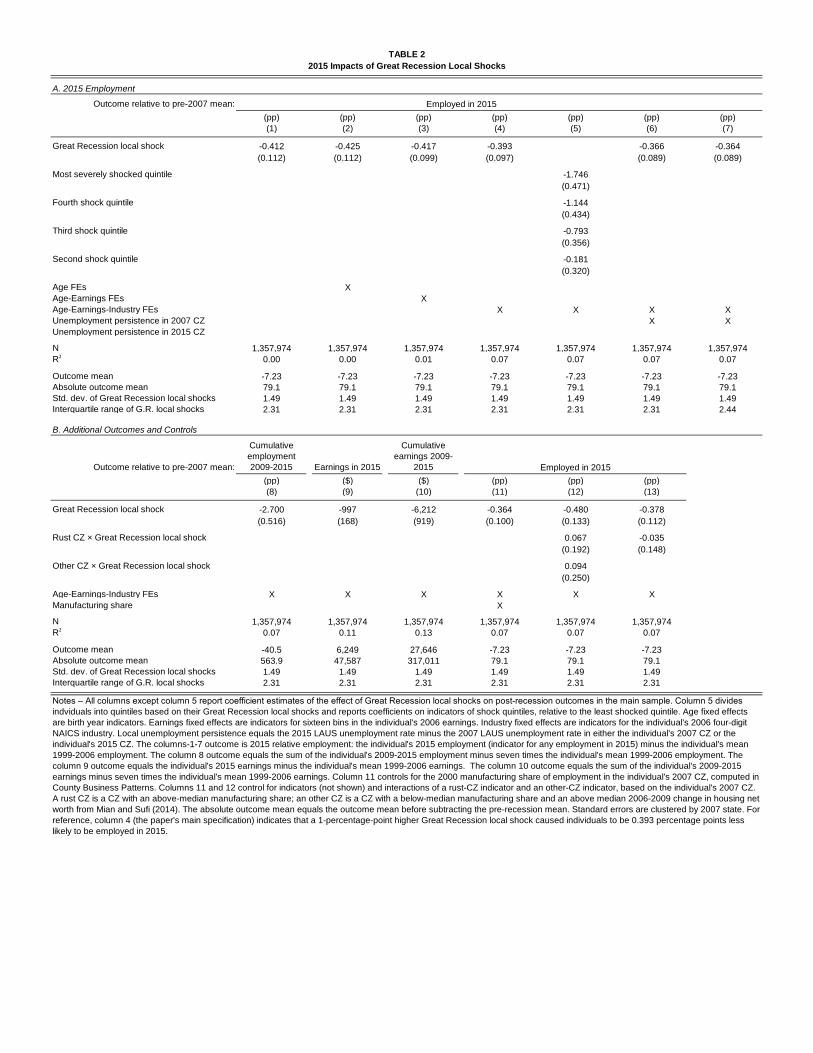
A. 2015 Employment

Outcome relative to pre-2007 mean:

(pp) (pp) (pp) (pp) (pp) (pp) (pp)

(1) (2) (3) (4) (5) (6) (7)

Great Recession local shock -0.412 -0.425 -0.417 -0.393 -0.366 -0.364

(0.112) (0.112) (0.099) (0.097) (0.089) (0.089)

Most severely shocked quintile -1.746

(0.471)

Fourth shock quintile -1.144

(0.434)

Third shock quintile -0.793

(0.356)

Second shock quintile -0.181

(0.320)

Age FEs X

Age-Earnings FEs X

Age-Earnings-Industry FEs X X X X

Unemployment persistence in 2007 CZ X X

Unemployment persistence in 2015 CZ

N 1,357,974 1,357,974 1,357,974 1,357,974 1,357,974 1,357,974 1,357,974

R20.00 0.00 0.01 0.07 0.07 0.07 0.07

Outcome mean -7.23 -7.23 -7.23 -7.23 -7.23 -7.23 -7.23

Absolute outcome mean 79.1 79.1 79.1 79.1 79.1 79.1 79.1

Std. dev. of Great Recession local shocks 1.49 1.49 1.49 1.49 1.49 1.49 1.49

Interquartile range of G.R. local shocks 2.31 2.31 2.31 2.31 2.31 2.31 2.44

B. Additional Outcomes and Controls

Outcome relative to pre-2007 mean:

Cumulative

employment

2009-2015 Earnings in 2015

Cumulative

earnings 2009-

2015

(pp) ($) ($) (pp) (pp) (pp)

(8) (9) (10) (11) (12) (13)

Great Recession local shock -2.700 -997 -6,212 -0.364 -0.480 -0.378

(0.516) (168) (919) (0.100) (0.133) (0.112)

Rust CZ × Great Recession local shock 0.067 -0.035

(0.192) (0.148)

Other CZ × Great Recession local shock 0.094

(0.250)

Age-Earnings-Industry FEs X X X X X X

Manufacturing share X

N 1,357,974 1,357,974 1,357,974 1,357,974 1,357,974 1,357,974

R20.07 0.11 0.13 0.07 0.07 0.07

Outcome mean -40.5 6,249 27,646 -7.23 -7.23 -7.23

Absolute outcome mean 563.9 47,587 317,011 79.1 79.1 79.1

Std. dev. of Great Recession local shocks 1.49 1.49 1.49 1.49 1.49 1.49

Interquartile range of G.R. local shocks 2.31 2.31 2.31 2.31 2.31 2.31

Employed in 2015

Notes – All columns except column 5 report coefficient estimates of the effect of Great Recession local shocks on post-recession outcomes in the main sample. Column 5 divides

indviduals into quintiles based on their Great Recession local shocks and reports coefficients on indicators of shock quintiles, relative to the least shocked quintile. Age fixed effects

are birth year indicators. Earnings fixed effects are indicators for sixteen bins in the individual's 2006 earnings. Industry fixed effects are indicators for the individual's 2006 four-digit

NAICS industry. Local unemployment persistence equals the 2015 LAUS unemployment rate minus the 2007 LAUS unemployment rate in either the individual's 2007 CZ or the

individual's 2015 CZ. The columns-1-7 outcome is 2015 relative employment: the individual's 2015 employment (indicator for any employment in 2015) minus the individual's mean

1999-2006 employment. The column 8 outcome equals the sum of the individual's 2009-2015 employment minus seven times the individual's mean 1999-2006 employment. The

column 9 outcome equals the individual's 2015 earnings minus the individual's mean 1999-2006 earnings. The column 10 outcome equals the sum of the individual's 2009-2015

earnings minus seven times the individual's mean 1999-2006 earnings. Column 11 controls for the 2000 manufacturing share of employment in the individual's 2007 CZ, computed in

County Business Patterns. Columns 11 and 12 control for indicators (not shown) and interactions of a rust-CZ indicator and an other-CZ indicator, based on the individual's 2007 CZ.

A rust CZ is a CZ with an above-median manufacturing share; an other CZ is a CZ with a below-median manufacturing share and an above median 2006-2009 change in housing net

worth from Mian and Sufi (2014). The absolute outcome mean equals the outcome mean before subtracting the pre-recession mean. Standard errors are clustered by 2007 state. For

reference, column 4 (the paper's main specification) indicates that a 1-percentage-point higher Great Recession local shock caused individuals to be 0.393 percentage points less

likely to be employed in 2015.

TABLE 2

2015 Impacts of Great Recession Local Shocks

Employed in 2015

Outcome relative to pre-2007 mean:

(pp) (pp) (pp) (pp) (pp) (pp) (pp) (pp) (pp) (pp) (pp) (pp) (pp)

(1) (2) (3) (4) (5) (6) (7) (8) (9) (10) (11) (12) (13)

Great Recession local shock -0.393 -0.394 -0.344 -0.344 -0.397 -0.439 -0.412 -0.381 -0.404 -0.399 -0.400 -0.397 -0.477

(0.097) (0.096) (0.090) (0.093) (0.098) (0.093) (0.098) (0.095) (0.095) (0.096) (0.115) (0.129) (0.125)

Main controls X X X X X X X X X X X X X

Gender X

Number of kids X

Married X

Home ownership X

CZ size X

CZ pre-2007 size growth X

Cross-CZ commuting X

Max UI duration 2007-2015 X

Minimum wage change 2007-2015 X

Exclude if invalid industry code X X

Exclude if construction/manufacturing X

Instrumented with birth state shock X

N 1,357,974 1,357,974 1,357,974 1,357,974 1,357,974 1,357,974 1,357,974 1,357,974 1,357,974 1,357,974 741,165 579,553 1,357,974

R2 0.07 0.08 0.09 0.08 0.07 0.07 0.07 0.07 0.07 0.07 0.11 0.10 0.07

Outcome mean -7.23 -7.23 -7.23 -7.23 -7.23 -7.23 -7.23 -7.23 -7.23 -7.23 -7.20 -6.69 -7.23

Absolute outcome mean 79.1 79.1 79.1 79.1 79.1 79.1 79.1 79.1 79.1 79.1 73.9 70.8 79.1

Std. dev. of G.R. local shocks 1.49 1.49 1.49 1.49 1.49 1.49 1.49 1.49 1.49 1.49 1.49 1.49 1.49

Interquartile range of G.R. local shocks 2.31 2.31 2.31 2.31 2.31 2.31 2.31 2.31 2.31 2.31 2.31 2.31 2.31

Notes – This table adds controls, sample restrictions, or instruments to the specification underlying Table 2 column 4, reprinted here in column 1. Column 2 controls for the individual's gender. Column 3 controls for the individual's 2006

number of kids (fixed effets for 0, 1, or 2+ kids). Column 4 controls for the individual's 2006 marital status. Column 5 controls for individual's 2006 home ownership status. Colums 6-10 control for CZ-level characteristics. Column 6 controls

for the individual's 2007 CZ's size, equal to the CZ's total employment in 2006 as reported in Census's County Business Patterns (CBP). Column 7 controls for the individual's 2007 CZ's size growth, equal to the CZ's log change in CBP

employment from 2000 to 2006. Column 8 controls for the individual's 2007 CZ's share of workers who work outside of the CZ, computed from the 2006-2010 American Community Surveys. Column 9 controls for the individual's 2007

state's maximum unemployment insurance duration over years 2007-2015. Column 10 controls for the individual’s 2007 state’s 2015 minimum wage minus that state’s 2007 minimum wage. Column 11 excludes 2006 W-2 earners without

an industry code and 2006 contractors and thus restricts the sample to those for whom 2006 industry is correctly measured: 2006 W-2 earners with a valid industry code and the 2006 nonemployed. Column 12 further excludes individuals

employed in construction or manufacturing in 2006. Column 13 instruments the individual's Great Recession local shock using the mean of the Great Recession local shock in the individual's birth state. Standard errors are clustered by

2007 state.

TABLE 3

Robustness of the 2015 Employment Impacts

Employed in 2015

A. Main Specifications

Outcome relative to pre-2007 mean:

(pp) (pp) (pp) (pp) (pp) (pp) (pp) (pp)

(1) (2) (3) (4) (5) (6) (7) (8)

Great Recession local shock -0.414 -0.426 -0.398 -0.407 -0.359 -0.340 -0.339

(0.118) (0.119) (0.102) (0.094) (0.080) (0.063) (0.061)

Most severely shocked quintile -1.496

(0.308)

Fourth shock quintile -1.416

(0.298)

Third shock quintile -0.968

(0.288)

Second shock quintile -0.366

(0.298)

Age FEs X

Age-Earnings FEs X

Age-Earnings-Industry FEs X

Age-Earnings-Firm FEs X X X X

Unemployment persistence in 2007 CZ X X

Unemployment persistence in 2015 CZ

N 865,954 865,954 865,954 865,954 865,954 865,954 865,954 865,954

R20.00 0.00 0.02 0.03 0.07 0.15 0.15 0.15

Outcome mean -9.80 -9.80 -9.80 -9.80 -9.80 -9.80 -9.80 -9.80

Absolute outcome mean 81.8 81.8 81.8 81.8 81.8 81.8 81.8 81.8

Std. dev. of Great Recession local shocks 1.49 1.49 1.49 1.49 1.49 1.49 1.49 1.49

Interquartile range of G.R. local shocks 2.31 2.31 2.31 2.31 2.31 2.31 2.31 2.44

B. Additional Outcomes and Controls

Outcome relative to pre-2007 mean:

Cumulative

employment

2009-2015 Earnings in 2015

Cumulative

earnings 2009-

2015

(pp) ($) ($) (pp) (pp) (pp)

(9) (10) (11) (12) (13) (14)

Great Recession local shock -2.504 -422 -2,777 -0.365 -0.589 -0.405

(0.430) (134) (606) (0.081) (0.111) (0.095)

Rust CZ × Great Recession local shock 0.258 0.069

0.144 0.115

Other CZ × Great Recession local shock 0.414

0.251

Age-Earnings-Firm FEs X X X X X X

Manufacturing share X

N 865,954 865,954 865,954 865,954 865,954 865,954

R20.15 0.21 0.23 0.15 0.15 0.15

Outcome mean -51.5 2,356 8,381 -9.80 -9.80 -9.80

Absolute outcome mean 590.0 33,381 225,554 81.8 81.8 81.8

Std. dev. of Great Recession local shocks 1.49 1.49 1.49 1.49 1.49 1.49

Interquartile range of G.R. local shocks 2.31 2.31 2.31 2.31 2.31 2.31

Notes – This table replicates Table 2 in the retail chain sample. See the notes to that table for details. Firm is an indicator for the individual's 2006 firm (a retail chain firm). The retail chain sample is

reweighted to match the main sample as described in the note to Figure 5.

Employed in 2015

TABLE 4

2015 Impacts of Great Recession Local Shocks ‒ Retail Chain Sample

Employed in 2015

Outcome (relative or

absolute): Employed

Migrated

outside 2007

CZ

Employed in

2007 CZ

Employed

outside 2007

CZ Earnings

Earnings in

2007 CZ

Earnings

outside 2007

CZ UI income SSDI income

(pp) (pp) (pp) (pp) ($) ($) ($) ($) ($)

(1) (2) (3) (4) (5) (6) (7) (8) (9)

Effect in 2007 0.087 0.000 0.087 0.000 -205 -205 0 14.3 -3.8

(0.106) (0.106) (115) (115) (12.2) (8.9)

Effect in 2008 -0.099 0.036 -0.098 -0.001 -508 -480 -28 36.3 -3.4

(0.079) (0.119) (0.077) (0.006) (108) (108) (11) (15.6) (9.4)

Effect in 2009 -0.349 0.109 -0.321 -0.028 -750 -687 -63 94.0 0.5

(0.080) (0.208) (0.077) (0.012) (129) (127) (18) (32.1) (11.8)

Effect in 2010 -0.403 0.209 -0.367 -0.037 -807 -736 -71 83.9 2.6

(0.074) (0.272) (0.074) (0.017) (131) (125) (30) (32.1) (13.0)

Effect in 2011 -0.387 0.248 -0.339 -0.048 -840 -745 -94 43.1 7.5

(0.072) (0.296) (0.071) (0.022) (119) (105) (35) (24.3) (13.7)

Effect in 2012 -0.373 0.244 -0.324 -0.049 -890 -784 -106 19.9 9.8

(0.075) (0.334) (0.076) (0.026) (141) (117) (45) (20.1) (15.2)

Effect in 2013 -0.434 0.180 -0.365 -0.069 -960 -810 -149 7.7 13.0

(0.089) (0.382) (0.091) (0.032) (147) (108) (56) (16.3) (17.0)

Effect in 2014 -0.360 0.134 -0.322 -0.038 -968 -799 -169 -3.0 15.7

(0.100) (0.422) (0.101) (0.031) (197) (135) (84) (9.9) (17.7)

Effect in 2015 -0.393 0.073 -0.338 -0.055 -997 -786 -211 -5.9 19.6

(0.097) (0.456) (0.100) (0.042) (168) (108) (101) (8.9) (18.8)

TABLE 5

Time Series of Adjustment Margins

Notes – This table expands on the specifications of Table 2 column 4 and column 9, whose results are reprinted here in the bottom rows of columns 1 and 5. Each cell

reports the coefficient on the Great Recession local shock variable from a separate regression in which the outcome uses the post-recession year indicated in the row,

instead of exclusively using 2015 as in Table 2. Every regression uses the same 1,357,974 observations underlying Table 2. The column 1 outcome of relative employment is

defined in Table 2, varying the post-recession year between 2007 and 2015. The column 2 outcome is an indicator for out-migration, equal to the individual's year-t CZ being

different from her 2007 CZ. Columns 3 and 4 separate the column 1 outcome for year t into two outcomes: employment in year t in the individual's 2007 CZ and employment

in year t outside the individual's 2007 CZ, each minus mean 1999-2006 employment. The column 5 outcome is defined in Table 2. Columns 7 and 8 separate the column 5

outcome analogously to columns 3-4. The column 8 outcome is the individual's unemployment insurance benefits in year t . The column 9 outcome is the individual's Social

Security Disability Insurance benefits in year t . Standard errors are clustered by 2007 state. See Online Appendix Table 2 for pre-trends.

A. Disability Insurance Receipt in Main Sample

Outcome:

SSDI receipt in

2015

2015 relative

employment-or-

SSDI-receipt

2015 relative

employment

2015 relative

employment

2015 relative

employment

(pp) (pp) (pp) (pp) (pp)

(1) (2) (3) (4) (5)

Great Recession local shock 0.071 -0.265 -0.577 -0.628 -0.605

(0.145) (0.099) (0.126) (0.118) (0.125)

Main controls X X X X X

Exclude if invalid industry code X X

Exclude if construction/manuf. X

N 1,357,974 1,357,974 1,001,543 573,493 396,377

R2 0.12 0.09 0.11 0.17 0.15

Outcome mean 6.22 -2.28 -10.12 -10.45 -9.85

Absolute outcome mean 6.22 84.06 84.12 83.11 83.20

Outcome:

UI receipt

sometime

2007-2014

2015 relative

employment-or-UI-

receipt-sometime-

2007-2014

2015 relative

employment

Relative non-

employment 2007-

2014

2015 relative

employment

2013-2015 relative

employment

(pp) (pp) (pp) (pp) (pp) (pp)

(6) (7) (8) (9) (10) (11)

Great Recession local shock 1.431 -0.019 -0.354 0.487 -0.057 -0.285

(0.418) (0.121) (0.099) (0.122) (0.111) (0.101)

UI receipt sometime 2007-2014 -2.734

(0.142)

Main controls X X X X X X

Employment 2007-2012 X

N 1,357,974 1,357,974 1,357,974 1,357,974 1,357,974 1,357,974

R2 0.16 0.06 0.08 0.08 0.26 0.07

Outcome mean 25.6 -2.8 -7.2 3.0 -7.2 -1.2

Absolute outcome mean 25.6 83.6 79.1 3.0 79.1 85.2

TABLE 6

Additional Outcomes

Notes – The table reports estimates of the specification in Table 11 column 4 with alternative outcomes, samples, and/or controls. Column 1 replicates the

main specification using the outcome of an indicator for 2015 receipt of Social Security Disability Insurance. Column 2 replicates the main specification using

the outcome of an indicator for 2015 employment or 2015 SSDI receipt, minus the individual's mean employment 1999-2006. Column 3 replicates the main

specification and columns 4-5 replicate Table 13 columns 11-12 in the mass layoffs sample. Column 6 replicates the main specification using the outcome of

an indicator for unemployment insurance (UI) benefit receipt at some point 2007-2014. Column 7 replicates column 2 but uses UI receipt 2007-2014 in place

of 2015 SSDI receipt. Column 8 replicates the main specification, controlling for UI receipt sometime 2007-2014. Column 9 replicates the main specification

using the outcome of an indicator for having any year of nonemployment 2007-2014, minus an indicator for having any year of nonemployment 1999-2006.

Column 10 replicates the main specification while controlling for indicators of employment in each year 2007-2012. Column 11 replicates the main

specification using the outcome of an indicator for employment in any year 2013-2015, minus the individual's mean employment 1999-2006. Standard errors

are clustered by 2007 state.

C. Layoffs and Nonemployment in Main Sample

B. Employment Impacts in Mass Layoffs Sample

ONLINE APPENDIX

57

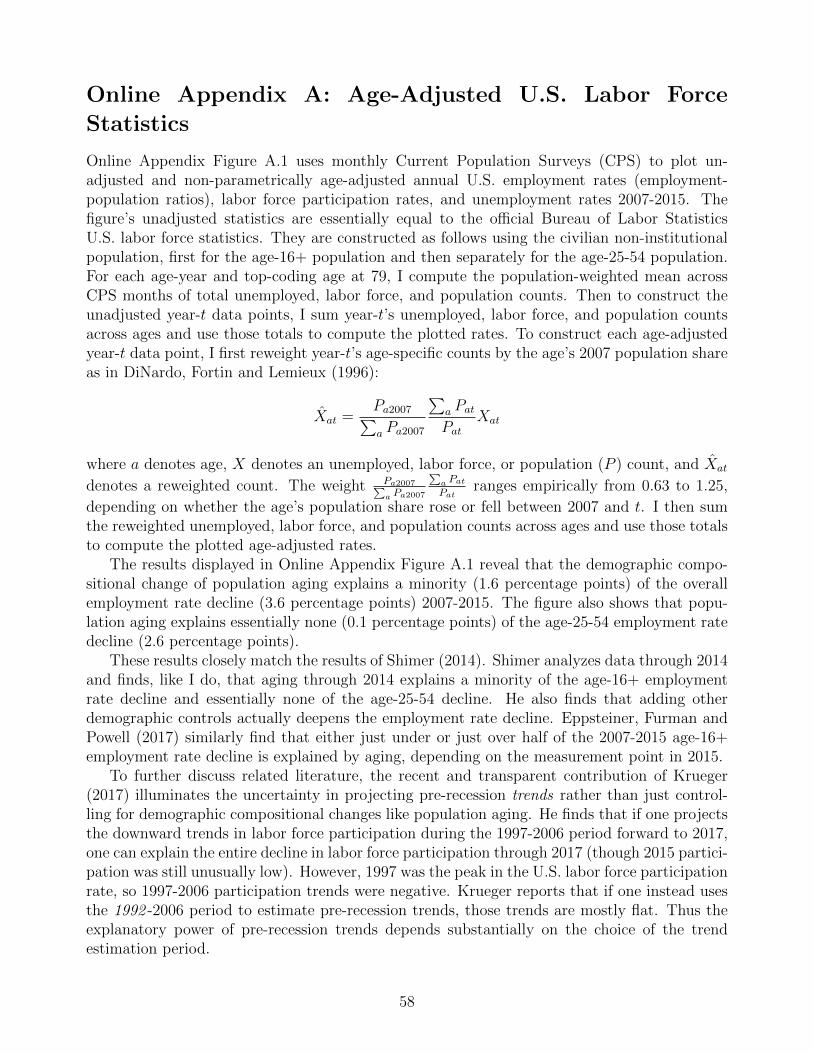
Online Appendix A: Age-Adjusted U.S. Labor Force

Statistics

Online Appendix Figure A.1 uses monthly Current Population Surveys (CPS) to plot un-adjusted and non-parametrically age-adjusted annual U.S. employment rates (employment-population ratios), labor force participation rates, and unemployment rates 2007-2015. Thefigure’s unadjusted statistics are essentially equal to the official Bureau of Labor StatisticsU.S. labor force statistics. They are constructed as follows using the civilian non-institutionalpopulation, first for the age-16+ population and then separately for the age-25-54 population.For each age-year and top-coding age at 79, I compute the population-weighted mean acrossCPS months of total unemployed, labor force, and population counts. Then to construct theunadjusted year-t data points, I sum year-t’s unemployed, labor force, and population countsacross ages and use those totals to compute the plotted rates. To construct each age-adjustedyear-t data point, I first reweight year-t’s age-specific counts by the age’s 2007 population shareas in DiNardo, Fortin and Lemieux (1996):

Xat =Pa2007∑a Pa2007

∑a Pat

Pat

Xat

where a denotes age, X denotes an unemployed, labor force, or population (P ) count, and Xat

denotes a reweighted count. The weight Pa2007∑a Pa2007

∑a Pat

Patranges empirically from 0.63 to 1.25,

depending on whether the age’s population share rose or fell between 2007 and t. I then sumthe reweighted unemployed, labor force, and population counts across ages and use those totalsto compute the plotted age-adjusted rates.

The results displayed in Online Appendix Figure A.1 reveal that the demographic compo-sitional change of population aging explains a minority (1.6 percentage points) of the overallemployment rate decline (3.6 percentage points) 2007-2015. The figure also shows that popu-lation aging explains essentially none (0.1 percentage points) of the age-25-54 employment ratedecline (2.6 percentage points).

These results closely match the results of Shimer (2014). Shimer analyzes data through 2014and finds, like I do, that aging through 2014 explains a minority of the age-16+ employmentrate decline and essentially none of the age-25-54 decline. He also finds that adding otherdemographic controls actually deepens the employment rate decline. Eppsteiner, Furman andPowell (2017) similarly find that either just under or just over half of the 2007-2015 age-16+employment rate decline is explained by aging, depending on the measurement point in 2015.

To further discuss related literature, the recent and transparent contribution of Krueger(2017) illuminates the uncertainty in projecting pre-recession trends rather than just control-ling for demographic compositional changes like population aging. He finds that if one projectsthe downward trends in labor force participation during the 1997-2006 period forward to 2017,one can explain the entire decline in labor force participation through 2017 (though 2015 partici-pation was still unusually low). However, 1997 was the peak in the U.S. labor force participationrate, so 1997-2006 participation trends were negative. Krueger reports that if one instead usesthe 1992 -2006 period to estimate pre-recession trends, those trends are mostly flat. Thus theexplanatory power of pre-recession trends depends substantially on the choice of the trendestimation period.

58

In a simultaneous equation system with many variables, Aaronson, Cajner, Fallick, Galbis-Reig, Smith and Wascher (2014) find, like Krueger’s 1997-2006-based projection, that mostof the age-adjusted labor force participation rate decline can be explained by projecting pre-recession trends. However, Hall (2014) suggests that the ACFGSW specification is likely tobe sensitive to reasonable amendments, and at least two projections have proven too aggres-sive. The earlier similar analysis of Aaronson, Fallick, Figura, Pingle and Wascher (2006)projected such a large labor force participation rate decline that the actual U.S. participationrate exceeded their projection after 2014 (ACFGSW Figure 1). Similarly, ACFGSW projectedcontinued and substantial age-16+ labor force participation declines after the second quarterof 2014 (their Table 6) while the actual age-16+ participation rate remained constant betweenthen and the time of this writing (the second quarter of 2017).

All told, this appendix’s analysis finds that the demographic compositional change of popu-lation aging explains a minority of the overall employment rate decline 2007-2015 and essentiallynone of the age-25-54 decline. A review of other work suggests that the explanatory power andaccuracy of pre-recession trends depend substantially on the trend estimation specification.This paper’s main finding supports the view that 2015 employment rates would have beenhigher in lieu of the Great Recession.

Online Appendix B: State-Level Shocks

This online appendix extensively details the autoregressive system of Blanchard and Katz (1992,BK) used to define state-level Great Recession shocks in Section 2 and elaborates on Figure 2’shistorical comparisons of state-level shock adjustment. The online replication kit contains dataand code that generate the results.

Section 2 estimates state-level adjustment using the updated data used in BK: the annualLocal Area Unemployment Statistics (LAUS) series of employment, population, unemploy-ment, and labor force participation counts 1976-2015 for 51 states (the 50 states plus theDistrict of Columbia) produced by the Bureau of Labor Statistics (BLS).38 Variable defini-tions are standard and pertain to the age-16-and-over civilian noninstitutional population.39

BLS compiles LAUS counts from the Current Population Survey (CPS), Current EmploymentStatistics (CES) survey, and state administrative unemployment insurance counts—blended tofilter maximal signal from noise using empirical Bayes techniques.40 Online Appendix Table 3displays summary statistics.

I employ BK’s canonical empirical model of state labor market outcomes to compute Great

38LAUS are the official data used to allocate federal transfers across states. The series is limited historicallyby the lack of Current Population Survey participation statistics for most states prior to 1976.

39Age is defined at the time of survey; LAUS figures effectively evenly weight underlying monthly surveys. Seehttp://www.bls.gov/bls/glossary.htm for full definitions of labor force status. Employment is roughly defined asworking for pay or being temporarily absent from regular work at any point in the reference week. Unemploymentis roughly defined as having had no employment in the reference week but being available for work and havinglooked for work in the preceding month. Labor force equals employment plus unemployment.

40Since LAUS had not yet been produced, BK effectively constructed their own version of LAUS 1976-1990 using the Geographic Profile of Employment (comprising CPS unemployment and population counts),employment counts from the CES (comprising formal employment counts), and an ad-hoc CPS-based imputationfor self-employment (population was implied). LAUS-based results on the original BK time series are essentiallyidentical to BK’s published results.

59

Recession employment shocks for each state. BK imagine a simple spatial equilibrium in whichU.S. states experience one-time random-walk shocks to global demand for their locally producedand freely traded goods. Those shocks induce endogenous migration responses of workers andfirms via transitory wage changes until state employment rates return to their steady states.BK aimed to estimate the nature and speed of those responses: do workers move out or dojobs move in, and over what horizon? To guide their implementation, BK observe empiricallythat states differ in long-run employment and population growth rates (e.g. perhaps partly dueto steady improvements in air conditioning that made the Sun Belt steadily more attractive)and in long-run unemployment rates and participation rates (e.g. due to industrial mix andretiree population differences) relative to the national aggregate. Thus an attractive modelof the evolution of state labor market outcomes may feature stationary employment growth,a stationary unemployment rate, and a stationary participation rate (and thus a stationaryemployment rate) for each state relative to the corresponding national aggregates.

BK implement such a model. They characterize state adjustment to idiosyncratic state-levellabor demand shocks by estimating the following log-linear autoregressive system in relativestate employment growth, unemployment rates, and participation rates:

∆ lnEst = αs10 + α11 (2) ∆ lnEs,t−1 + α12 (2) ˜lnE/Ls,t−1 + α13 (2) ˜lnL/P s,t−1 + εEst˜lnE/Lst = αs20 + α21 (2) ∆ lnEst + α22 (2) ˜lnE/Ls,t−1 + α23 (2) ˜lnL/P s,t−1 + εE/Lst˜lnL/P st = αs30 + α31 (2) ∆ lnEst + α32 (2) ˜lnE/Ls,t−1 + α33 (2) ˜lnL/P s,t−1 + εL/Pst

where E, L, and P denote levels of employment, the labor force, and population in state s inyear t; where ∆ denotes a first difference (year t’s value minus year t−1’s value); where ˜ denotesa difference relative to the year’s national aggregate value; and where (2) denotes a vector oftwo lags. Thus the first dependent variable (“relative state employment”) is the first differenceof log state employment minus the first difference of log aggregate employment. The second(“relative state unemployment”) is the log of one minus the state unemployment rate minus thelog of one minus the aggregate unemployment rate. The third (“relative state participation”)is the log of the state participation rate minus the log of the aggregate participation rate.Relative state population is the implied residual. Each equation includes a state fixed effect.I follow BK in weighting states equally rather than by population. Under these assumptions,the autoregressive coefficients characterize the speed of the average state’s convergence to itssteady state following an unforecasted change in state labor demand: coefficients close to oneimply slow convergence while coefficients close to zero imply fast convergence.41

41The BK system embodies four substantive assumptions. First, unforecasted changes in relative state em-ployment growth εEst affect contemporaneous relative employment growth, relative unemployment, and relativeparticipation, but unforecasted changes in relative state unemployment and participation do not effect con-temporaneous values of the other outcomes. This feature allows the system to be estimated independently viaordinary least squares. It reflects the assumption that εEst primarily reflects changes in labor demand ratherthan supply—supported in the data by negative values of εEst typically being followed by state wage declinesrather than increases. Second, each state-year outcome is differenced by the year’s aggregate value, so thebehavior of the system is assumed to be independent of aggregate levels. Third, serial correlation is assumedto be affine in two lags, which limits the estimation sample to years 1978 and beyond (three and four lagsdeliver similar results). Fourth, outcomes are assumed to be stationary, i.e. to converge in the long run totime-invariant state-specific steady-state values relative to national aggregates. State fixed effects are motivatedby cross-decadal persistence in the outcomes. Formal stationarity tests are underpowered and inconclusive in

60

For each state, I estimate a 2008 and a 2009 employment growth forecast error within theBK system and refer to their sum as its Great Recession employment shock. Specifically, Ifirst estimate the BK system coefficients using sample years 1978-2007 (i.e. using years 1976-

2007 with two lags). I then compute each state’s 2008 employment shock εEs,2008, equal to the

state’s actual relative employment growth ∆ lnEs,2008 minus the relative employment growthpredicted by the state’s actual data through 2007 and the estimated coefficients. For example,a state that experienced 2008 relative employment growth equal to the system forecast basedon its history through 2007 would have a 2008 shock equal to zero. I similarly compute each

state’s 2009 employment shock εEs,2009, equal to the state’s actual relative employment growth

∆ lnEs,2009 minus the relative employment growth predicted by the state’s actual data through

2008 and the estimated coefficients. I refer to each state’s vector { εEs,2008,εEs,2009} as the state’s

Great Recession employment shocks and to the sum of the vector’s elements as the state’s GreatRecession employment shock.

To understand these shocks empirically, Online Appendix Table 4 lists each state’s GreatRecession employment shock. The standard deviation of state-level shocks over the GreatRecession (2.74) was similar to the standard deviation of state-level shocks over the early-1980s(1980-1982) recession (2.73) computed similarly (detailed below).42 Recall that shocks areeffectively defined as 2007-2009 employment level changes relative to the state’s own trend andthe national aggregate. Thus a state can have a negative Great Recession employment shockeither because its employment growth relative to the aggregate became moderately negativeafter a history of fast growth (e.g. Arizona) or because employment growth became verynegative after a history of slow growth (e.g. Michigan). Furthermore, just over half of statesnaturally experienced a positive Great Recession shock, since shocks are measured relativeto the aggregate. The table displays patterns familiar from popular news accounts and earliereconomics work: Sun Belt states like Arizona, California, and Florida as well as Rust Belt stateslike Michigan and Indiana experienced severe Great Recession shocks relative to other states.As two focal examples, Arizona’s shock equals −2.24% while Texas’s shock equals +1.30%.

Online Appendix Figures A.4A-B plot actual mean responses (solid lines) of state labormarket outcomes to 2007-2009 shocks versus mean historical benchmark responses (dottedlines) to a −1% shock, following BK’s exposition. Forty-one percent of the average state’s2007-2009 shock arrived in 2008 while 59% arrived in 2009. To generate historical bench-mark predicted responses 2008-2015, I therefore feed the BK system the employment resid-

ual vector { εEs,2008,εEs,2009} = {−.41,−.59} and—for maximum comparability to BK’s original

benchmarks—use coefficients estimated on the original sample years 1978-1990; panel C plotsupdated benchmarks.43 Note that by construction in the BK system, the predicted meanresponse to a −1% shock is the negative of the predicted mean response to a +1% shock.44

short time series (BK). Stationarity here is best motivated by spatial arbitrage priors, no rise in the standarddeviation of outcomes before 2007, and employment rate stationarity after previous recessions (Figure 2A).

42The standard deviation of shocks is smaller outside aggregate recession years.43Strictly speaking, I feed the system the vector {−.41,−.59} shrunk multiplicatively by a constant such that

the 2007-2009 change in relative employment is −1% after system feedback effects.44Online Appendix Figures A.4A-B correspond closely to BK’s Figure 7, with year 2009 corresponding to year

negative one in BK’s Figure 7. The graphs differ in that the −1% shock in Online Appendix Figures A.4A-Bis spread out over two years instead of one and in that Online Appendix Figures A.4A-B use the official LAUSseries that was released after BK.

61

Panel A’s benchmark predictions depict BK’s core lesson: in response to a −1% changein a state’s employment relative to the state’s trend and the national aggregate, the 1978-1990 experience predicts that the state’s population would rapidly fall by 1% relative to thestate’s trend and the national aggregate—such that the state’s employment rate returns to itssteady-state level relative to the aggregate in five years. Colloquially, residents move out andothers stop moving in, rather than jobs moving in or residents remaining nonemployed—andthe adjustment completes quickly. Economically, the adjustment process has been understoodto embody a simple mechanism: a state (e.g. Michigan) experiences a one-time random-walkcontraction in global consumer demand for its locally produced traded good (e.g. cars), whichinduces a local labor demand contraction and wage decline, which in turn induces a local laborsupply (population) contraction, which then restores the original local wage and employmentrate.

The mean actual response series equals the estimated mean responses of outcomes acrossstates within each year. To construct the series, I first compute forecast errors for each year2008-2015 and for each system outcome, using actual data through 2007 and the coefficientsfrom the 1978-2007-estimated system.45 Denote these forecast errors for each variable-state-year {ηEst, η

E/Lst , η

L/Pst }. I then regress these forecast errors on 2007-2009 shocks in year-by-year

regressions:46

ηEst = εEs,2008δEt + εEs,2009ζ

Et , ∀t

ηE/Lst = εEs,2008δ

E/Lt + εEs,2009ζ

E/Lt , ∀t

ηL/Pst = εEs,2008δ

L/Pt + εEs,2009ζ

L/Pt , ∀t

This specification is flexible in that it allows for the 2008 and 2009 employment shocks to havearbitrary additive effects on each subsequent year’s outcomes. The δ and ζ coefficients are meanactual responses of each outcome in each year to 2007-2009 shocks. I multiply these coefficients

by the −1% 2007-2009 shock { εEs,2008,εEs,2009} = {−.41,−.59} to obtain the plotted mean actual

response series.Panel A shows that on a slight lag, mean actual relative population responded identically

to Great Recession shocks as in the historical benchmark—falling by 1% between 2007 and2014, matching the initial 1% employment decline. However, actual relative employment keptdeclining such that employment rates remained diverged across space at nearly their 2009 levels:for every −1% decline in relative state employment 2007-2009, the relative state employmentrate was 0.45 percentage points lower in 2015 than it was in 2007. This 0.45 percentage-pointemployment rate deficit is similar to the 0.48 percentage-point deficit that prevailed in 2009.Hence, employment rates had far from converged across space by 2015, contrary to history-based predictions. Panel B separates the employment rate response into the unemploymentrate response and the labor force participation rate response. The graph shows that actualrelative unemployment rates converged across space as in the historical benchmark, while actualparticipation rates remained diverged in a stark departure from the historical benchmark.

Online Appendix Figure A.4C shows that updating the historical benchmark to more recent

45That is, I compute 2008-2015 baseline predictions for how each state’s outcomes would have evolved inthe absence of 2007-2009 shocks based on data through 2007 and the estimated coefficients, and then subtractpredictions those 2008-2015 baseline predictions from actual 2008-2015 values.

46For 2008, only the 2008 employment shock is included as a regressor.

62

data does not alter the conclusion that post-2007 employment rate convergence was unusuallyslow and incomplete. The figure plots the estimated response of the average state’s employmentrate to a −1% employment shock, based on estimating the BK system on three different LAUSsample ranges: 1978-1990 (the original BK time range, reprinted from panels A-B), 1991-2007, and 1978-2015.47 Both the 1978-1990- and 1991-2007-based predictions exhibit five-year convergence of the state’s employment rate to its steady-state level relative to the theaggregate. The 1978-2015-based prediction exhibits substantially slower convergence but stillexhibits majority employment rate convergence 2009-2015, in contrast to reality.48 Hence, the2007-2015 employment rate divergence is exceptional even relative to fully-updated convergencepredictions.

Finally, Figure 2A (documented in the main text) shows that the slow convergence afterGreat Recession shocks was unusual not merely relative to average historical responses but alsorelative to the aftermath of the two previous recessions for which a long post-recession timeseries is available.49 Online Appendix Figure A.5 repeats Figure 2A for the labor force participa-tion rate, unemployment rate, employment growth, and population growth. The participationand unemployment graphs are constructed exactly as the employment rate graph in Figure2A. To create the employment growth graph, I first compute each state’s steady state valuefor relative employment growth by using the 1978-2007-estimated BK coefficients and solvingthe BK system assuming all variables are constant. Then, for each state-year around each re-cession, I compute actual relative employment growth minus steady state relative employmentgrowth, cumulate this value beginning in year −5 (year −3 for the early-1980s recession, thefirst year available), and proceed to construct the graph exactly as done for employment rates.The population employment graph is constructed similarly. The graphs show that the unem-ployment rate and population growth adjustments to Great Recession employment shocks werebroadly similar to those after previous recessions’ shocks. However, the participation rate andemployment growth in severely shocked states exhibited no recovery from 2009 levels relativeto mildly shocked states, in stark contrast to the aftermath of the early-1980s and early-1990srecessions.

Online Appendix C: Cross-State Employment Gap

This online appendix documents the computation of the 2.01 million cross-state employmentgap statistic reported in Section 2. The employment gap is defined as total 2015 employmentin severely shocked states minus total 2015 employment in mildly shocked states—minus thedifference that would have prevailed if the pre-recession severe-mild employment rate differencehad prevailed in 2015 at 2015 state populations. 2.01 ≈ .01635/2 × 250.5 = 2.05, where 1.635percentage points is the population-weighted equivalent to the 1.736-percentage-point severe-mild 2015 employment rate deficit plotted in Figure 1B and where 250.5 million was 2015total population. This formula is not exact because population was not exactly evenly divided

47See Beyer and Smets (2014) for an earlier re-estimation of the BK system augmented with multi-level factormodeling to compare U.S. and Europe population responses. See Dao, Furceri and Loungani (2017) for an earlierre-estimation augmented with instruments to find stronger population responses during aggregate recessions.

48Slower convergence likely derives from unique divergence after 2007 as well as from alleviated small-samplestationarity bias in a larger sample (e.g. Hurwicz 1950).

49The post-2001-recession experience exhibited incomplete convergence before being interrupted by positivelycorrelated 2007-2009 shocks.

63

between the two state groups, since the unweighted shock median was used to define the groups.For reference, the exact 2.01 figure is computed as follows.

On average 2002-2007, the population-weighted employment rate in severely shocked statesminus that in mildly shocked states equaled −0.885 percentage points. In 2015, severelyshocked states had an adult civilian noninstitutional population of 142.0 million with a 58.25%population-weighted employment rate while mildly shocked states had an adult civilian non-institutional population of 108.5 million with a 60.77% population-weighted employment rate(note that 58.25 − 60.77 + 0.885 = −1.635). Then the full-convergence employment rate inseverely shocked states (e∗S) and in mildly shocked states (e∗M) solve:

e∗S − e∗M = −.00885

142.0× e∗S + 108.5× e∗M = 142.0× .5825 + 108.5× .6077

where the first equation imposes full employment rate convergence between severely shockedand mildly shocked states to the pre-2007 difference and the second equation imposes equal-ity between the full-convergence aggregate employment level (and rate) and the actual 2015aggregate employment level (and rate).

The solution is e∗S = 58.96% and e∗M = 59.84%. This implies that 1.005 (= 141.99 ×(.58959− .58251)) million fewer residents of severely shocked states in 2015 were employed thanthere would have been had state employment rates returned to their pre-2007 differences atactual 2015 populations and the actual 2015 aggregate employment rate. Likewise, 1.006 (=108.52×(.60771−.59844)) million more residents of mildly shocked states in 2015 were employedthan there would have been had state employment rates returned to their pre-2007 differencesaround the actual 2015 aggregate employment rate. Hence relative to the counterfactual of fullconvergence of state employment rates to their pre-2007 differences at actual 2015 populations,a 2.01-million-person employment gap between severely shocked and mildly shocked statesremained in 2015.

Online Appendix D: Empirical Design in Potential Out-

comes

This online appendix details a binary version of the paper’s empirical design in potential out-comes. Consider identical local areas c that experienced in 2007-2009 a binary Great Reces-sion local shock—severe or mild—and no other 2007-2009 shocks. Denote these areas severelyshocked or mildly shocked. SEV EREc(i2007) ∈ {0, 1} indicates whether an individual i livedin 2007 in a severely shocked area. EMPLOY EDi2015(1) ∈ {0, 1} indicates i’s potential 2015employment if her 2007 local area was severely shocked, and EMPLOY EDi2015(0) ∈ {0, 1}indicates i’s potential 2015 employment if her 2007 local area was mildly shocked. To alignnotation simply with the text’s main outcome, assume that all individuals were employed inevery year 1999-2006.

Define the causal effect βi of i’s 2007 CZ’s Great Recession local shock on i’s 2015 employ-ment as the difference in the worker’s potential employment: βi ≡ EMPLOY EDi2015(1) −EMPLOY EDi2015(0). Note that βi could be zero for some skill types and negative for oth-ers, for example if only construction or routine workers are affected by a severe local shock(Jaimovich and Siu 2013, Hershbein and Kahn 2016). But βi excludes all nationwide changes

64

that do not vary with local shock severity. The mean E[βi] ≡ β in a relevant sample of workersis my causal effect of interest, which I refer to as the causal effect of Great Recession localshocks.

If workers were randomly assigned in 2007 across local areas, then one could consistentlyestimate β as the unconditional observed employment rate difference in longitudinal dataas: E[EMPLOY EDi2015|SEV EREc(i2007) = 1]− E[EMPLOY EDi2015|SEV EREc(i2007) = 0].Lacking random assignment, I assume empirically that workers were as good as randomly as-signed conditional on a rich observed vector of pre-2007 characteristics Xi2006:(

EMPLOY EDi2015(0), EMPLOY EDi2015(1))⊥ SEV EREc(i2007) | Xi2007c(i2007)

Then β can be consistently estimated as the conditional observed employment rate differencein longitudinal data:

E[EMPLOY EDi2015|SEV EREc(i2007) = 1,Xi2007c(i2007)] −E[EMPLOY EDi2015|SEV EREc(i2007) = 0,Xi2007c(i2007)] −

= E[EMPLOY EDi2015(1)− EMPLOY EDi2015(0)].

Two appendix graphs help to justify the interpretation of β presented in Section 3.1. Myinterpretation of β is sensible because severely shocked and mildly shocked areas exhibited rela-tively similar pre-recession trends in the outcomes of interest (shown in Section 4.1) and becausepost-2010 unemployment rates converged monotonically across severely shocked and mildlyshocked areas (Figure 2A and Online Appendix Figure A.2A). Moreover, adverse 2010-2015industry-based shift-share shocks are not positively correlated with adverse Great Recessionlocal shocks (Online Appendix Figure A.2B).

Online Appendix E: Longitudinal Data

This online appendix provides additional details on the longitudinal linked-employer-employeedata described in Section 3.

First, the universe of business tax returns used is the universe of C-corporate (Form 1120),S-corporate (Form 1120S), and partnership (Form 1065) tax returns. Businesses that file othertypes of tax returns employ a small share of U.S. workers.

Second, Form 1099-MISC data on independent contractor employment are missing in 1999.Results are very similar when omitting 1999 data.

Third, many retail chain firms are missing from the retail chain sample, both because ofsubsidiaries and franchises as described in Section 3 and also because a (likely small) number offirms outsource their W-2 administration to third-party payroll administration firms that listtheir own EINs on W-2s. Nevertheless, the retail chain sample includes very large nationwidechains.

Fourth and also specific to the retail chain sample, the filing ZIP code on a firm’s busi-ness income tax return typically but not always refer to the business’s headquarters ZIP code.Excluding workers at the business’s headquarters is useful because headquarters workers mayperform systematically different tasks than workers at other establishments and thus may pos-sess different human capital even conditional on baseline earnings. I therefore conservatively

65

exclude firms’ workers living in the CZ with the largest number of the firm’s workers livingthere, as well as the CZ with the largest number of the firm’s workers living there as a share ofthe total number of workers living there.

Fifth and also specific to the retail chain sample, I consider a firm to have operated in aCZ in 2006 if it employed at least ten stably located workers who lived in the CZ—defined asindividuals of any age and citizenship with a W-2 from the firm in all years 2005-2007 and thesame residential CZ in all years 2005-2007 based on those W-2s’ payee (residential) ZIP codes.It is necessary to define CZ operations using more than one year of W-2 data because W-2payee ZIP code refers to the worker’s ZIP code in January of the year after employment. Thatfeature implies that almost all firms would appear to have operations in every large CZ if onewere to use only 2006 W-2s to identify CZ operations, since many workers move to large cities.

In Section 3.3, I noted that transition of affected workers to self-employment likely does notexplain the results. An appendix graph helps to justify that conclusion: Current PopulationSurvey data indicate that changes in state self-employment rates since 2007 were unrelated tochanges in state formal employment rates (Online Appendix Figure A.3).

66

Figure A.1: The Age-Adjusted U.S. Employment Rate Decline

Ages 16+ Ages 25-54

A . Employment Rate D. Employment Rate

5859

6061

6263

Empl

oym

ent r

ate

(%)

2007 2008 2009 2010 2011 2012 2013 2014 2015

Unadjusted Age-adjusted

7576

7778

7980

Empl

oym

ent r

ate

(%)

2007 2008 2009 2010 2011 2012 2013 2014 2015

Unadjusted Age-adjusted

B. Labor Force Participation Rate E. Labor Force Participation Rate

6364

6566

67La

bor f

orce

par

ticip

atio

n ra

te (%

)

2007 2008 2009 2010 2011 2012 2013 2014 2015

Unadjusted Age-adjusted

8181

.582

82.5

83La

bor f

orce

par

ticip

atio

n ra

te (%

)

2007 2008 2009 2010 2011 2012 2013 2014 2015

Unadjusted Age-adjusted

C. Unemployment Rate F. Unemployment Rate

56

78

910

Une

mpl

oym

ent r

ate

(%)

2007 2008 2009 2010 2011 2012 2013 2014 2015

Unadjusted Age-adjusted

45

67

89

Une

mpl

oym

ent r

ate

(%)

2007 2008 2009 2010 2011 2012 2013 2014 2015

Unadjusted Age-adjusted

Notes: This figure uses monthly Current Population Surveys (CPS) to plot unadjusted and non-parametricallyage-adjusted annual U.S. employment rates (employment-population ratios), labor force participation rates,and unemployment rates 2007-2015 for the civilian non-institutional population. The unadjusted statisticsare essentially equal to the official Bureau of Labor Statistics U.S. labor force statistics. The age-adjustedstatistics reweight each age-year’s annual total unemployment, labor force, and population by the age group’s2007 population share as in DiNardo, Fortin and Lemieux (1996) before summing across ages and computingthe displayed rates. See Online Appendix A for details.

67

Figure A.2: Evidence against Positively Correlated Independent Shocks

A. Unemployment Rates by Shock Severity 2007-2015

46

810

1214

Une

mpl

oym

ent R

ate

(%)

2007 2008 2009 2010 2011 2012 2013 2014 2015 2016

Mildly shocked CZs Severly schocked CZs

B. 2010-2015 Shift-Share Shocks vs. Great Recession Local Shocks

1516

1718

19

2010

-201

5 sh

ift-s

hare

sho

ck (%

)

2 3 4 5 6 7 8Great Recession local shock (pp)

Notes: Panel A uses LAUS county-level data, aggregated to the CZ-level, to plot monthly mean unemploymentrates 2007-2015 in severely shocked CZs (those with above median Great Recession local shocks) and mildlyshocked CZs (all other CZs). Data points are weighted by CZ population. The post-2001-recession experienceexhibited incomplete convergence before being interrupted by positively correlated 2007-2009 shocks. PanelB plots 2010-2015 CZ-level shift-share shocks versus Great Recession local shocks. The shift-share shocks areconstructed analogously to Bartik (1991) using County Business Patterns data as follows. Each CZ’s shift-shareshock equals the projected 2010-2015 percentage change in the CZ’s employment based on leave-one-CZ-outnationwide changes in employment by three-digit NAICS industry categories. That is, a CZ c’s shift-share

shock equals: SHIFTSHARESHOCKc =∑

j

(Ejc2010∑j′ Ej′c2010

×∑

c′ 6=c Ejc′2015−∑

c′ 6=c Ejc′2010∑c′ 6=c Ejc′2010

)where j denotes a

three-digit industry and Ejct denotes total employment in industry j in CZ c in year t. The graph bins CZs intoventiles (five-percentile-point bins) by their Great Recession local shock and then plots the 2007-population-weighted mean of the 2010-2015 shift share shock within each bin. If CZs that were severely shocked duringthe Great Recession had subsequently experienced additional adverse shift-share shocks 2010-2015 related tothe CZs’ industrial compositions, Panel B would have exhibited a negative relationship instead of the displayedinsignificant positive relationship.

68

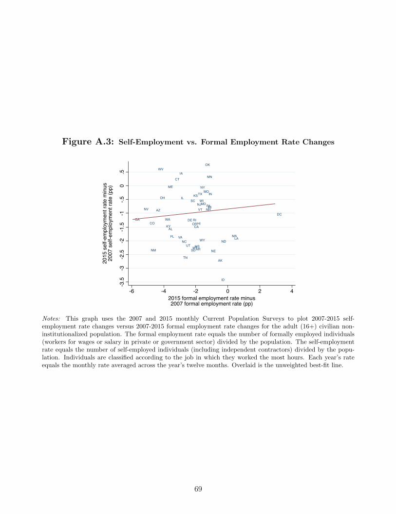
Figure A.3: Self-Employment vs. Formal Employment Rate Changes

AL

AK

AZ

AR

CACO

CT

DEDC

FL

GAHI

ID

ILIN

IA

KS

KY

LA

ME

MD

MA

MI

MN

MS

MO

MTNE

NV NHNJ

NM

NY

NC ND

OH

OK

OR

PA

RI

SC

SD

TN

TX

UT

VT

VA

WA

WV

WI

WY

-3.5

-3-2

.5-2

-1.5

-1-.5

0.5

2015

sel

f-em

ploy

men

t rat

e m

inus

2007

sel

f-em

ploy

men

t rat

e (p

p)

-6 -4 -2 0 2 42015 formal employment rate minus2007 formal employment rate (pp)

Notes: This graph uses the 2007 and 2015 monthly Current Population Surveys to plot 2007-2015 self-employment rate changes versus 2007-2015 formal employment rate changes for the adult (16+) civilian non-institutionalized population. The formal employment rate equals the number of formally employed individuals(workers for wages or salary in private or government sector) divided by the population. The self-employmentrate equals the number of self-employed individuals (including independent contractors) divided by the popu-lation. Individuals are classified according to the job in which they worked the most hours. Each year’s rateequals the monthly rate averaged across the year’s twelve months. Overlaid is the unweighted best-fit line.

69

Figure A.4: State Employment Rate Persistence after 2007-2009 Shocks

A. Employment, Population, and B. Participation, Unemployment, andEmployment Rate after −1% Shock Employment Rates after −1% Shock

-2-1

.5-1

-.50

Dev

iatio

n fro

m tr

end

and

aggr

egat

e

2007 2008 2009 2010 2011 2012 2013 2014 2015

Pred. employment (%) Act. employment (%)Pred. population (%) Act. population (%)Pred. employment rate (pp) Act. employment rate (pp)

-.5-.2

50

.25

.5

Dev

iatio

n fro

m tr

end

and

aggr

egat

e

2007 2008 2009 2010 2011 2012 2013 2014 2015

Pred. unemployment rate (pp) Act. unemployment rate (pp)Pred. participation rate (pp) Act. participation rate (pp)Pred. employment rate (pp) Act. employment rate (pp)

C. Actual 2007-2014 Employment Rate

-.6-.5

-.4-.3

-.2-.1

0

Dev

iatio

n fro

m tr

end

and

aggr

egat

e (p

p)

2007

2008

2009

2010

2011

2012

2013

2014

2015

2016

2017

2018

2019

2020

2021

2022

2023

2024

Year relative to shock

Pred. based on 1978-1990 Pred. based on 1991-2007Pred. based on 1978-2015 Actual 2007-2015

Notes: The dotted lines of panels A-B plot benchmark history-based predictions for state-level responses toa −1% 2007-2009 state-level employment shock, based on estimating Blanchard-Katz’s (1992) autoregressivesystem of state labor market outcomes using LAUS data on the original sample range 1978-1990. The solidlines plot mean actual state-level responses based on reduced-form regressions of 2008-2014 state-level outcomeson 2007-2009 state-level shocks. Panel C plots the mean actual employment rate response series from panelsA-B alongside predicted employment rate series based on three estimation time ranges: 1978-1990 (as in panelsA-B), 1991-2007, and 1978-2014. See Online Appendix B for more details.

70

Figure A.5: Great Recession Local Convergence Compared to History: Extended

A. Labor Force Participation Rate B. Unemployment Rate

-2-1

.5-1

-.50

.5

Parti

cipa

tion

rate

diff

eren

ce b

etw

een

seve

rely

shoc

ked

and

mild

ly s

hock

ed s

tate

s (p

p)

-5 -4 -3 -2 -1 0 1 2 3 4 5 6 7 8 9 10Year relative to recession

1980-1982 recession1990-1991 recession2007-2009 recession

-.50

.51

1.5

22.

5

Une

mpl

oym

ent r

ate

diffe

renc

e be

twee

n se

vere

lysh

ocke

d an

d m

ildly

sho

cked

sta

tes

(pp)

-5 -4 -3 -2 -1 0 1 2 3 4 5 6 7 8 9 10Year relative to recession

1980-1982 recession1990-1991 recession2007-2009 recession

C. Employment Growth D. Population Growth

-8-6

-4-2

0

Empl

oym

ent g

row

th: s

ever

ely

shoc

ked

stat

esm

inus

mild

ly s

hock

ed s

tate

s (lo

g pt

s)

-5 -4 -3 -2 -1 0 1 2 3 4 5 6 7 8 9 10Year relative to recession

1980-1982 recession1990-1991 recession2007-2009 recession

-5-4

-3-2

-10

1

Popu

latio

n gr

owth

: sev

erel

y sh

ocke

d st

ates

min

us m

ildly

sho

cked

sta

tes

(log

pts)

-5 -4 -3 -2 -1 0 1 2 3 4 5 6 7 8 9 10Year relative to recession

1980-1982 recession1990-1991 recession2007-2009 recession

Notes: Panels A-B replicate Figure 2A for the labor force participation rate and unemployment rate. PanelsC-D display analogous graphs for employment growth and population growth. These latter panels require thateach state’s estimated steady state annual growth rate is subtracted from its actual annual growth, beforeconstructing the graphs exactly as in Panels A-B. See Online Appendix B and the notes to Figure 2.

71

Outcome:

Individual-level 2015 relative

employment (from tax data)

CZ-level estimated employment

effect (from tax data)

CZ-level 2015 relative employment

(from BLS LAUS and Census)

(pp) (pp) (pp)

(1) (2) (3)

Great Recession local shock -0.393 -0.381 -0.490

(0.097) (0.100) (0.115)

Main controls X

Main sample (individual-level) X

Published sample (CZ-level) X X

N 1,357,974 591 591

R2 0.07 0.10 0.09

ONLINE APPENDIX TABLE 1

Approximating the Main Result Using Published Data

Notes – This table shows that the paper's main estimate of the 2015 employment impact of Great Recession local shocks—which uses the main

sample's non-public individual-level data—can be well-approximated in CZ-level data published alongside this paper. Column 1 reprints the main

specification and estimate from Table 2 column 4. Columns 2-3 report coefficients from univariate CZ-level regressions weighted by the CZ's 2007

population as reported in Census's Annual County Resident Population Estimates of the total adult (16+) population, aggregated to the CZ level. The

column 2 outcome equals the estiamated coefficients on a vector of CZ fixed effects from estimating the main specification with Great Recession local

shock variable replaced by a vector of CZ fixed effects. Online Appendix Table 2 lists these estimated coefficients for the hundred largest CZs. The

column 3 outcome variable equals the CZ's 2015 adult employment rate minus the CZ's mean 1999-2007 employment rate, based on Census data and

Bureau of Labor Statistics Local Area Unemployment Statistics data: LAUS county-level 16+ civilian non-institutional employment aggregated to the CZ

level, divided by Census's CZ population estimate. Column 3 is restricted to the CZs available for column 2. Standard errors are clustered in column 1

by the individual's 2007 state and in columns 2-3 by the CZ's state. See the paper's Online Data Codebook and Online Data Tables for additional

details and published variables on the author's website.

Outcome (relative or

absolute): Employed

Migrated

outside 2000

CZ

Employed in

2000 CZ

Employed

outside 2000

CZ Earnings

Earnings in

2000 CZ

Earnings

outside 2000

CZ UI income SSDI income

(pp) (pp) (pp) (pp) ($) ($) ($) ($) ($)

(1) (2) (3) (4) (5) (6) (7) (8) (9)

Effect in 2000 -0.036 0.000 -0.036 0.000 72 72 0 0.6 0.4

(0.083) (0.083) (66) (66) (6.2) (3.9)

Effect in 2001 -0.094 -0.036 -0.093 -0.001 -74 -67 -7 10.6 0.3

(0.045) (0.166) (0.044) (0.003) (46) (42) (6) (9.2) (4.6)

Effect in 2002 -0.068 -0.047 -0.060 -0.008 -56 -47 -9 9.7 0.7

(0.018) (0.280) (0.017) (0.004) (26) (23) (5) (15.4) (5.4)

Effect in 2003 -0.044 -0.005 -0.036 -0.008 -26 -17 -10 10.2 0.6

(0.029) (0.361) (0.031) (0.007) (21) (20) (6) (15.9) (5.8)

Effect in 2004 0.031 0.077 0.030 0.001 1 6 -5 11.0 0.3

(0.039) (0.437) (0.036) (0.009) (36) (30) (12) (11.9) (6.6)

Effect in 2005 0.083 0.151 0.070 0.013 40 42 -1 6.8 -0.1

(0.061) (0.526) (0.053) (0.010) (66) (57) (22) (11.5) (7.3)

Effect in 2006 0.228 0.252 0.189 0.039 -15 1 -16 9.1 0.4

(0.135) (0.612) (0.116) (0.020) (118) (94) (36) (13.1) (9.1)

ONLINE APPENDIX TABLE 2

Adjustment Margins Pre-Trends

Notes – This table replicates Table 5 for years 2000-2006 and where each individual's Great Recession local shock equals the 2007-2009 percentage-point unemployment

rate change in the individual's 2000 CZ. See the notes to Table 5 for details.

Mean Standard Deviation

(1) (2)

Employment rate (%)

1978-2015 62.3 4.6

2007 64.1 3.9

2009 60.7 4.5

2015 60.4 4.4

Unemployment rate (%)

1978-2015 6.1 2.1

2007 4.4 1.0

2009 8.5 2.0

2015 5.0 1.1

Labor force participation rate (%)

1978-2015 66.3 4.1

2007 67.0 3.8

2009 66.3 4.0

2015 63.6 4.1

Number of states

Number of years

Number of observations (state-years)

Notes – This table lists summary statistics of the Bureau of Labor Statistics's Local Area

Unemployment Statistics (LAUS) state-year labor force statistics 1978-2015. The LAUS data cover

the adult (16+) civilian non-institutional population of the fifty states and the District of Columbia.

The employment rate is the ratio of employment to population. The unemployment rate is the ratio

of unemployed to labor force. The labor force participation rate is the ratio of labor force to

population.

ONLINE APPENDIX TABLE 3

Summary Statistics: State-Level Data

1,938

51

38

Great

Recession

Employment

Shock Rank State

Great

Recession

Employment

Shock

Change in

Employment

Rate

2007-2015

Great

Recession

Employment

Shock Rank State

Great

Recession

Employment

Shock

Change in

Employment

Rate

2007-2015

(pp) (pp) (pp) (pp)

(1) (2) (3) (4) (5) (6) (7) (8)

1 Nevada -6.46 -6.94 27 Washington 1.13 -5.21

2 Alabama -3.42 -5.54 28 New Hampshire 1.13 -2.03

3 Michigan -3.36 -2.74 29 Missouri 1.24 -1.42

4 Georgia -3.19 -7.09 30 Arkansas 1.26 -4.79

5 Delaware -3.14 -4.65 31 Texas 1.30 -2.06

6 Mississippi -3.04 -4.21 32 Virginia 1.56 -4.87

7 Utah -2.53 -4.31 33 Maryland 1.92 -2.79

8 Florida -2.40 -5.45 34 Louisiana 1.99 -2.41

9 South Carolina -2.35 -3.59 35 Massachusetts 2.06 -1.64

10 Arizona -2.24 -4.82 36 Alaska 2.26 -3.67

11 Idaho -2.20 -4.53 37 Minnesota 2.33 -2.24

12 North Carolina -2.15 -4.79 38 New Jersey 2.37 -3.21

13 Tennessee -1.56 -5.18 39 West Virginia 2.58 -4.18

14 Indiana -1.52 -2.45 40 Pennsylvania 2.68 -2.15

15 Hawaii -1.33 -4.27 41 New York 2.79 -2.28

16 Oregon -1.29 -4.33 42 Oklahoma 3.25 -1.90

17 California -0.63 -3.74 43 Connecticut 3.33 -3.33

18 New Mexico -0.57 -6.80 44 South Dakota 3.56 -3.98

19 Illinois -0.33 -4.02 45 Wyoming 3.85 -4.30

20 Ohio 0.05 -4.19 46 Kansas 4.35 -2.98

21 Montana 0.46 -3.45 47 Vermont 4.38 -2.93

22 Colorado 0.73 -5.15 48 Nebraska 4.77 -2.99

23 Wisconsin 0.75 -2.48 49 Iowa 5.00 -2.03

24 Rhode Island 0.81 -3.98 50 District of Columbia 5.44 0.94

25 Kentucky 0.90 -4.60 51 North Dakota 5.75 -2.48

26 Maine 1.09 -3.39

ONLINE APPENDIX TABLE 4

State-Level Great Recession Employment Shocks and 2007-2015 Employment Rate Changes

Notes – This table lists the Great Recession state-level employment shocks and 2007-2015 percentage-point changes in state-level employment

rates that underlie the severe-vs-mild-shock grouping of Figure 1B. See the notes to those figures and Online Appendix B for details. Severely

shocked states are listed on the left; mildly shocked states are listed on the right.