This is a manuscript version. The article has been accepted for publication

in the Journal of Public Economics.

Empty homes, longer commutes: the unintended

consequences of more restrictive local planning*

Paul Cheshire

London School of Economics &

Spatial Economics Research Centre: p.cheshire@lse.ac.uk

and

Christian A.L. Hilber

London School of Economics,

Centre for Economic Performance &

Spatial Economics Research Centre: c.hilber@lse.ac.uk

and

Hans R.A. Koster

Vrije Universiteit Amsterdam,

Tinbergen Institute &

Centre for Economic Policy Research &

Spatial Economics Research Centre: h.koster@vu.nl

This Version: 24th

August 2017

* Support from the Suntoya and Toyota International Centres for Economics and Related Disciplines

(STICERD) and the Spatial Economics Research Centre (SERC) are gratefully acknowledged. Hans Koster

acknowledges support from a VENI research grant from the Netherlands Organisation for Scientific Research.

We thank Gabriel Ahlfeldt, Jan Brueckner, Ed Coulson, Jeremiah Dittmar, Gilles Duranton, Stuart Gabriel,

Steve Gibbons, Raven Molloy, Alvin Murphy, Henry Overman, Olmo Silva, Stuart Rosenthal, Will Strange, Jos

Van Ommeren, Elisabet Viladecans-Marsal, Stephen Ross and conference/seminar participants at the Urban

Economics Association Meetings of the 2013 North American Meetings of the RSAI (Atlanta) and of the 2015

European Regional Science Association Congress (Lisbon), the 2015 AREUEA National Conference

(Washington, DC), the 2015 Conference on Housing Affordability at the UCLA (Los Angeles), the 2015 CEPR

Conference on Urban and Regional Economics (CURE) (Basel), the 2016 AREUEA-ASSA Conference (San

Francisco), the Urban and Regional Economics seminar (Paris) and the SERC/LSE seminar (London) for

helpful comments and suggestions. All errors are the sole responsibility of the authors. We also thank the Editor

and two anonymous referees for helpful comments and suggestions. Address correspondence to: Hans Koster,

Vrije Universiteit Amsterdam, De Boelelaan 1105, 1081 HV Amsterdam, The Netherlands; Phone: +31 20 59

894 37; E-mail: h.koster@vu.nl

© 2017. This manuscript version is made available under the CC-BY-NC-ND 4.0 license

http://creativecommons.org/licenses/by-nc-nd/4.0

Empty homes, longer commutes: the unintended

consequences of more restrictive local planning

Abstract

We investigate the impact of land use regulation on housing vacancy rates. Using a 30-year

panel dataset on land use regulation for 350 English Local Authorities (LAs) and addressing

potential reverse causation and other endogeneity concerns, we find that tighter local

planning constraints increase local housing vacancy rates: a one standard deviation increase

in restrictiveness causes the local vacancy rate to increase by 0.9 percentage points (23

percent). The same increase in local restrictiveness also causes a 6.1 percent rise in

commuting distances. The results underline the interdependence of local housing and labour

markets and the unintended adverse impact of more restrictive planning policies.

JEL classification: R13, R38

Keywords: residential vacancy rates, housing supply constraints, land use regulation.

1

1. Introduction

To an economist it might seem self-evident that vacancies in the housing stock are a natural

feature of how any market must work. There even are ‘uneaten’ apples in a well-functioning

fruit market. The labour market is very much more comparable to the housing market and

virtually all mainstream economists expect to observe at least frictional unemployment when

the labour market is in equilibrium (see Pissarides, 1985; Mortensen and Pissarides, 1994;

Pissarides, 1994). It is the same in any normally functioning housing market. In equilibrium

there must be vacant houses as people move and ‘house-hunt’, as people die or houses wait to

be demolished and sellers wait to find a buyer (Han and Strange, 2015).

But this view is often not shared by those who design buildings and influence urban policy or

with those who plan housing supply – at least in England. Even in what was then one of the

least restrictive English Regions, the East Midlands, in calculating how much land should be

allocated for housing to meet their estimate of their region’s ‘housing needs’, planners argued

that they could allocate less land because they assumed they would reduce the number of

vacant homes:

‘The annual average housing provision reflects a number of factors, transactional

vacancies in new stock (about 2%) add 7,000 to the requirement, but offset against

that is an assumption that vacancies in the existing stock should be reduced by a half

per-cent, which will bring 8,600 dwellings back into use.’ (Government Office for the

East Midlands, 2005, Appendix 4, p. 91).

It is surely true that using ones stock of capital more intensively is a way of increasing

efficiency. That is just how cut price airlines operate: they keep their seats full and their

aircraft in the air. They, however, had an analysis of how to achieve this. They did not just

assume planes would spend more of their lives in the air and seats would be fuller. Unless we

understand why houses are vacant we cannot rationally hope to reduce the number of vacant

houses just by being more restrictive. To help improve our understanding of the factors which

determine vacancy rates in the housing market, this paper investigates the causal, albeit

reduced-form, impact of regulatory restrictiveness. Moreover, since housing and labour

markets are interdependent, we also investigate the related issue of how local regulatory

restrictiveness affects the average commute distance of those working in the jurisdiction.

These are not the only outcomes of greater regulatory restrictiveness. We find that there are

other measurable effects apart from raised house prices, all apparently responses to poorer

housing market matching (discussed below); more households are in temporary homes,

crowding is greater, and in-migration lower.

These results stem from the insight that policy imposed restrictions on housing supply may

have two opposing effects.1 The first of these we call the ‘opportunity cost effect’. Tighter

1 Regulation may have more than two effects. We discuss one potential additional mechanism – a real options

argument – in section 3.7. If greater restrictiveness led to greater price volatility then under certain assumptions

this might induce owners to postpone renting or selling their properties, implying a higher vacancy rate

(Grenadier, 1995; 1996). Empirically, however, we can find no evidence that such a mechanism plays a

significant part in explaining what we find. Other mechanisms are also discussed in that section.

2

restrictions on supply imply fewer available houses and therefore more demand pressure for

existing homes, increasing house prices and thus the opportunity cost of keeping housing

empty. This will lead to a lower vacancy rate all else equal. If this ‘opportunity cost effect’

was the only effect at work, tighter supply constraints should unambiguously lower vacancy

rates.

There is however a second effect, which we refer to as the ‘mismatch effect’. Tighter supply

constraints not only reduce supply of new houses but also influence the composition and

adaptability of the bundle of attributes of both the existing housing stock and those of new

built homes. Over time the structure of households’ demand for housing attributes changes

because incomes rise, the demographic structure of the population changes and preferences

themselves may change. For example, as real incomes rise, so does the demand for certain

attributes depending on the varying income elasticity of demand for them.2 In addition there

may be demographic changes such as an increase in the proportion of single adults, which

mean that market preferences change.

If the attributes of the housing stock, as a consequence of planning constraints, cannot, or can

only more slowly adjust to these changes on the demand side, matching the demand for

housing attributes with the supply of those available will inevitably become more difficult.

Hence, in line with Wheaton (1990), mismatched households may have to stay longer in a

less restrictive housing market while searching in a more restrictive one, implying a relatively

lower vacancy rate in the less restrictive market and a higher vacancy rate in the more

restrictive one. Mismatched households may also take temporary accommodation and search

for longer in more restrictive markets or have to search further afield for a suitable home;

they become mismatched on the locational characteristics of houses implying longer

commutes.

Our aim in this paper is to determine the net effect of these two opposing forces – the

opportunity cost effect versus the mismatch effect – in order to identify the role that

regulatory restrictiveness plays in determining the vacancy rate in local housing markets. To

do so, we analyse panel data on housing vacancies from 1981 to 2011 for 350 English Local

Authorities (LAs), the basic local jurisdictional unit that implements planning policies and

approves or rejects individual planning applications. One key concern in this analysis is the

endogeneity of local planning restrictiveness. The stylised fact that policy makers and local

planners may respond to higher vacancy rates by restricting supply suggests possible reverse

causation. Regulatory constraints may also be endogenous to unobserved demand factors

(Hilber and Robert-Nicoud, 2013; Davidoff, 2016) and those demand factors may directly

affect vacancy rates. To account for possible reverse causation and omitted variable bias and

thus identify the causal effect of regulatory restrictiveness, we employ an instrumental

variable strategy by exploiting specific features of the British voting system which induces a

substantial ‘randomness’ of seats won (or lost) beyond the vote share. That is, we use the

share of Labour seats in LAs, controlling for the share of Labour votes in a flexible way, as

2 The income elasticity of demand for space both inside houses and in gardens seems to be particularly strong:

Cheshire and Sheppard (1998) estimate an elasticity of close to two.

3

an instrumental variable to identify local planning restrictiveness. One could query this

identification strategy because, for example, the political composition of an LA could

influence local government expenditures and those, in turn, might influence house prices and

vacancy rates. Based on a series of placebo regressions, we show that these alternative

explanations do not plausibly invalidate the main conclusions.

Our two key empirical findings are as follows. First, when we naively look at cross-sectional

data, we find a negative relationship between more restrictive local planning and local

vacancy rates, superficially appearing to confirm “planners’ assumptions”. However, when

we (i) use first differencing and so control for time-invariant unobservable characteristics, (ii)

properly account for the endogeneity of restrictiveness by instrumenting for it and (iii)

control for other relevant factors, more restrictive places have a significantly – and

substantially – higher vacancy rate. That is, the underlying causal relationship appears to be

exactly the opposite to that which planners assume. Based on our most rigorous empirical

specification, a one standard deviation increase in local regulatory restrictiveness causes the

average local vacancy rate to increase by about 0.9 percentage points (23 percent).

Second, we find that regulation-induced mismatch has spatial implications for labour

markets. Workers with jobs in LAs with more restrictive planning have to search for housing

they can afford and match their preferences further afield; so they are more likely to be

locationally mismatched and have to commute further. Using a similar approach to that used

for investigating the underlying relationship between the vacancy rate and restrictiveness we

find that a one standard deviation increase in local regulatory restrictiveness causes an

increase in average commuting distance of some 6.1 percent. We also provide additional

suggestive evidence relating to other proxies for mismatch, such as the share of crowded or

non-permanent properties and the share of migrants.

Our findings, therefore, strongly suggest that tighter local planning restrictiveness not only

leads to less efficient housing market matching but also this effect dominates the opportunity

cost effect, resulting in higher local vacancy rates overall and longer average commutes.

Hence, local efforts to reduce the number of vacant homes by imposing supply restrictions

have three unintended effects: they increase the local vacancy rate and they increase the

average commuting distance of those who work in the jurisdiction – thereby causing a

welfare cost. In addition, as the literature shows, they increase local house prices (see e.g.

Cheshire and Sheppard, 2002; Glaeser and Gyourko, 2003; Hilber and Vermeulen, 2016).

We proceed as follows. In the next section we discuss in more depth the link between land

use regulation and mismatch in the housing market and how that affects the local vacancy

rate and the average commuting distance. We then describe our data and set out our main

results. The final section draws conclusions.

2. Land use regulation, housing market search and vacant housing

The price of housing services is a function of both demand and supply in the relevant local

markets. Various empirical studies document a positive effect of regulatory restrictiveness on

4

house prices (Cheshire and Sheppard, 2002; Glaeser and Gyourko, 2003; Glaeser et al.,

2005a; b; Quigley and Raphael, 2005; Ihlanfeldt, 2007; Hilber and Vermeulen, 2016).

What these studies do not consider is the fact that, on the seller’s side, it takes time to sell a

house and, on the buyer’s side, search for a new house is costly too. These search frictions

lead to housing vacancies (Merlo and Ortalo-Magné, 2004; Han and Strange, 2015). It has

been documented – and our data also suggest – that housing vacancies are not constant across

space and time and depend on the characteristics and preferences of households living in a

housing market, as well as on those of the location such as characteristics that are systematic

of persistently weak housing demand (Rosen and Smith, 1983; Gabriel and Nothaft, 1989;

Gabriel and Nothaft, 2001; Deng et al., 2003; Molloy, 2014). However, the impact of land

use restrictions on housing vacancies has not yet been studied.

In the context of this paper we use data on local jurisdictions – in Britain, LAs – which we

refer to as local housing markets.3 On the demand side, households often search in a local

housing market while still living in another local market, for example due to changes in

where they work (Mulalic et al., 2014; Koster and Van Ommeren, 2017). On the supply side,

the characteristics of housing are the result of both the characteristics of new build housing

and the adaptation of the characteristics of the existing stock.

The degree of regulatory restrictiveness influences the characteristics of new construction and

of the existing stock in very great detail. Both new construction and significant changes to the

characteristics of existing houses – converting loft to living space, for example – likely

require ‘development control’ permission. This is the responsibility of the LA’s Planning

Committee made up of locally elected politicians. This decision making process tends to be

politicised and unlike a Zoning or Master Planning system, such as in force in the US or in

most of Continental Europe, decisions are not very predictable.

As noted in the introduction, planning induced housing supply restrictions will have two

opposing effects on the housing vacancy rate: an ‘opportunity cost effect’ and a ‘mismatch

effect’. The opportunity cost effect works via restrictions of supply reducing the availability

of land for development (see for example Cheshire and Sheppard, 2005, or Hilber and

Vermeulen, 2016). This reduces the rate of new building and so over time the size of the

stock of housing relative to demand within the market. This, all else equal, increases prices

and thus the opportunity cost of keeping housing vacant. The effect of this is unambiguously

to reduce vacancy rates. It will also be likely to increase price volatility.

However, more restrictive planning policies will also change the bundle of attributes on offer

and, other things equal, slow the rate of adaptation of housing characteristics to changes in

3 It might be argued that Travel to Work Areas (TTWA) approximate more closely to spatial housing markets

but as our results demonstrate, the geographical extent of both housing and labour markets is jointly determined.

Planning policy is implemented by the local jurisdiction, the LA, so it is only by using these as our units of

analysis that the relationship between restrictiveness and commuting distances can be revealed. Not only do

TTWAs not correspond to any political jurisdiction but our finding on the impact of planning restrictiveness on

distance commuted shows their boundaries are partially determined by the policy actions of their constituent

jurisdictions.

5

the structure of demand with respect to them – the mismatch effect. The latter effect is

expected to increase vacancy rates. This will come about via two separate forces, one

working on the characteristics of new build and the other on the adaptation of the

characteristics of the existing stock of houses.

The first force may imply that new build houses become smaller, more distant from jobs and

are more likely to be in the form of flats or terraced houses, because there is less land

available for dwellings. The second force arises because the structure of demand for housing

characteristics changes over time and to accommodate this, the characteristics of the existing

stock of housing need to be constantly adjusted. For example, entry to the best state schools

in Britain is determined by the exact location of houses. As the relative standing of different

schools changes over time, people seeking to ‘buy’ entry to better state schools will want

more bedroom space in the best schools’ catchment areas. However, the more restrictive is

the LA, the more difficult it will be to adapt existing houses to provide more space or for

developers to build additional family housing near better schools.

Another example is that as more cars have been bought (car ownership has increased 13-fold

since the current form of land use planning in England was introduced in 1947 and doubled

since our vacancy data starts in 1981, Department for Transport, 2013), the demand for

garages and off street parking has increased. Such examples of ways in which the demand for

housing attributes changes over time could be increased almost indefinitely. However, what it

means is that if the supply and demand for the structural characteristics of housing are to be

efficiently matched to each other, there will need to be constant adaptation of the

characteristics of the existing stock of houses. So more restrictive LAs will slow the

adaptation of the existing stock to (changes in) the structure of demand for housing attributes.

Over time, in more restrictive LAs the characteristics of new and existing housing available

will be less adapted to preferences of households. Hence, other things equal, if people have a

(strong) idiosyncratic preference for locations and house type (e.g. a double-earner household

with children that needs at least two-bedrooms and garden space), they will spend more time

searching for housing that matches their preferences. When households live in a less

restrictive housing market while searching in the more restrictive local market, this will imply

a decrease in the vacancy rate in the former and an increase in the latter housing market.4 In

other words, given idiosyncratic preferences, households stay longer in the ‘wrong’ places.

This may imply that younger people live longer with their parents in ‘crowded’ properties, or

that households are induced to stay in temporary accommodation while searching. Because

the housing stock does not match their current preferences, this implies a higher vacancy rate,

other things equal, in the more restrictive housing market. We provide some evidence on

4 In the Web Appendix we demonstrate this in a standard search model setting, building on the seminal paper by

Wheaton (1990). Using numerical simulations, we formally demonstrate that under realistic parameter

assumptions an increase in the (relative) regulatory restrictiveness in a particular market increases the local

vacancy rate in that market (and lowers it in the comparably less restrictive market), even with perfectly

inelastic total demand for housing.

6

some of these different symptoms of mismatch in Section 3.6 where we look at how

regulation influences the share of non-permanent homes and ‘crowded’ properties.

We discuss also a more obvious measure of mismatch in Section 3.4: commuting distances

from the workplace in the LA. We do indeed find that for workers in more restrictive LAs

commuting distances increase significantly. This result is consistent with house hunters

finding it more difficult to match their preferences in more restrictive local housing markets

so becoming ‘mismatched’ locationally. This has interesting implications for the boundaries

of local labour markets – they appear to be determined not just by transport costs but also by

local planning policies – and how these affect the total supply of housing and the supply of

individual housing characteristics. Because households may decide not to move to the desired

more restricted place, the share of in-migrants is expected to be lower in the more restrictive

housing market. We provide evidence for the latter in Section 3.6.

The well-documented fact that tighter local regulation leads to higher prices is indicative that

the opportunity cost effect may be important in determining local vacancy rates. However,

we lack evidence on the importance of the offsetting mismatch effect. Thus the net effect of

local regulatory restrictiveness on local vacancy rates is ambiguous. The empirical analysis

that follows aims to identify this net effect while eliminating alternative explanations.

One may question whether changes in vacancy rates are a sufficient statistic when one is

interested in the welfare effects of land use regulation. We do not argue that vacancy rates in

general are a sufficient statistic. However, when one is specifically interested in the change in

welfare due to an increase in mismatch caused by more restrictive local planning, an increase

in the vacancy rate (beyond the natural rate) is a sufficient statistic for the former.

In line with a large labour market literature on matching, and as demonstrated by Koster and

Van Ommeren (2017), from a welfare perspective housing search may be either too low or

too high. However, when search is too low, that is caused by an externality for sellers: if

buyers search more they will find a suitable property sooner, thereby reducing the time on the

market and the associated costs for the seller. Buyers do not take this into account when

increasing search effort. However, a regulation-induced increase in vacancy rates while

increasing search effort, neither reduces sales times, nor increases matching quality, so the

welfare effects are unambiguously negative.

This is important because planning policies that aim to reduce vacancies by reducing new

construction but end up leaving more houses empty, cause an under-utilisation of a major

capital asset. According to ONS by the end of 2013 houses accounted for 61% of the UK’s

net worth: up from 48.7% 20 years previously (ONS, 2016). So the capital stock represented

by housing is very significant indeed and so its underutilisation represents a significant

economic inefficiency.

The effects on commuting are important in their own right as again they represent a welfare

loss resulting from increased difficulty of matching.

Of course planning policies per se have the potential to increase social welfare via correcting

market failures and we are not claiming here that our evidence on the effect of land use

regulation on vacancy rates and commuting distances in isolation suggests that local planning

7

restrictions reduce net welfare. However, there is evidence at least for the UK and the US that

an increase in the restrictiveness of planning policy (from current levels) has a net negative

effect on welfare (see Cheshire and Sheppard, 2002 for the UK and Turner et al., 2014 for the

US). In this context, our finding that more restrictive local planning increases the local

vacancy rate and commuting distance via raising mismatch in the local housing market, adds

to the alleged net negative effect on welfare. Both effects (on vacancy rates and commuting

distances) have been ignored in the literature so far.

3. Empirical analysis

3.1 Data and descriptive statistics

Our data come from several sources. The vacancy rates are from the UK Census for the years

1981, 1991, 2001 and 2011.5 For the first three Census years we have information on the

number of vacant dwellings and we are able to distinguish between primary dwellings and

second homes.6 The 2011 Census reported only information on the number of unoccupied

dwellings including second homes. To estimate vacancies for 2011 in the most consistent way

possible, therefore, we assume that the share of second homes remained constant between

2001 and 2011. In a robustness check we use an alternative dataset for vacancy rates

(available for 2001 and 2011 only) to test whether our findings are sensitive to this

adjustment. The latter dataset is provided by the Department of Communities and Local

Government (DCLG) using the LA returns for the Council Tax.7

Our measures of regulatory restrictiveness come from the DCLG’s Planning Statistics.

Following the literature, our key measure is the refusal rate for major residential projects

available for each LA on an annual basis. The refusal rate for ‘major’ projects is defined as

the share of applications for residential developments of ten or more dwellings that is refused

by an LA in any year during the process of ‘development control’. We calculate this for each

LA using data on all applications and refused applications of major developments for the

5 The Census does not distinguish between short-term and long-term vacant housing units. Molloy (2014) points

out that in the United States, long-term vacancies are on average rare but there are substantial spatial

differences. Our data do not allow us to explore differences between short-term and long-term vacancies.

However, it is worth pointing out that due to the extremely inflexible planning system in England, overbuilding

is highly unlikely anywhere in the country. Long-term vacancies as a consequence of weak housing demand will

likely be concentrated in the north of the country and the change in the unemployment rate will likely capture

the effect of declining areas in our empirical analysis. 6 The Census uses the term ‘household space’, which is a space taken by one household, including that of just

one person. Almost no household shares facilities like bathrooms (less than 0.1 percent), implying that the

number of (vacant) household spaces is essentially the same as the number of (vacant) dwellings. Hence, in

what follows, we will refer to dwellings as household spaces. 7 The cross-sectional correlation between the 2001 Census and the DCLG data is 0.68, indicating that there are

non-trivial differences in the measurement of vacant dwellings arising from the different methodologies. As is

discussed later, this hardly affects our results however.

8

Census year itself plus the two years preceding it.8 In what follows we call this variable the

refusal rate.

As a proxy for local (housing) demand we use LA-level male weekly earnings for the period

from 1981 to 2011. Our earnings data come from the Annual Survey of Hours and Earnings

(ASHE) for 2001 and 2011 and from the New Earnings Survey (NES) for 1981 and 1991. We

obtained the ASHE data at the LA-level but the NES data for earlier years are only available

at the county and London borough level. We then geographically matched all earnings data to

the LA-level and deflated the nominal earnings figures by the Retail Price Index to obtain

real earnings. For more details on the data and procedures used, see Hilber and Vermeulen

(2016).

A number of other factors may influence vacancy rates, in particular housing tenure,

demographics and socio economic characteristics. We obtain these control variables from the

Population Censuses. Our list of controls includes the local homeownership rate.

Homeowners tend to move less often than renters, and this is likely to be reflected in higher

vacancy rates for rental housing. We also control for the share of council housing. Because

rents of council houses are usually below market value, there are waiting lists for them. This

is likely to imply a shorter duration of vacancies (Pawson and Kintrea, 2002). However, this

effect could be offset to the extent councils have less efficient housing management.

The Population Censuses also provide data on the share of people between 30 and 64 and the

share of elderly, 65 and over. Young people may be more flexible in their housing choices

than older people, and they may be less selective because they are more income constrained

or have lower search costs (perhaps because of lower opportunity costs of time) leading to

lower vacancy rates in LAs where there are proportionately more young adults. On the other

hand, younger people tend to have a higher mobility rate, leading to higher vacancy rates.

The mortality rate is of course highly correlated to the share of elderly. Death frequently

implies that houses become vacant and, moreover, because of probate and perhaps other

reasons (the new owner may not be a local resident or the house has suffered a period of

neglect so is more likely to need refurbishment) houses that become vacant on the death of

their owner are likely to remain vacant for longer. Other control variables derived from the

Population Censuses are the share unemployed, the share of highly educated, and the share of

residents with permanent illnesses.

As a proxy for mismatch and as a significant focus of interest in its own right, we gather data

on the average commuting distance from the workplace for all the Census years. The data

provide us with the share of people per commuting distance band (0-2 km, 2-5 km, etc.). We

then calculate the average commuting distance by taking the midpoint of each category and

weighting it by the number of persons in each category. We further gather data on other

variables that may relate to spatial mismatch from the Census, such as the share of crowded

8 In a sensitivity analysis – see Appendix 2 – we also use additional information on the refusal rate of minor

projects and show that our results are robust when we include this additional information.

9

properties, the share of shared properties, the share of migrants and the share of non-

permanent dwellings.

Our instrumental variable strategy employs information on the political composition of the

LA and local vote shares. We obtained the local election data from various sources: (i) the

British Local Election Database (1889-2003) compiled by Rallings and Thrasher (2004), (ii)

the Local Election Handbooks (1999 to 2008), (iii) the Local Elections Archive Project

(LEAP) (2006 to 2010) and (iv) the BBC (2009 to 2011). We do not have data on four LAs,

so these are excluded from the analysis, leaving us with a sample of 350 LAs and four Census

years (1981, 1991, 2001 and 2011).9 Since it might be argued that turnout is

unrepresentatively low at local elections in the sensitivity analysis, we also use data on

general elections, by matching each Census year to the nearest general election year (i.e.,

1983, 1992, 2001 and 2010). The LA-level share of votes for the Labour party in the general

elections is derived from the British Election Studies Information System. For more

information on the election data, see Appendix 1.

We also gather data on net local expenditures from the Chartered Institute for Public Finance

and Accountancy (CIPFA) annual reports on finance and general estimates available for each

LA. We choose spending categories that remain robust over time, such as spending on

education, personal and social services (such as social care), highways, housing services,

local planning and the total local net expenditures. Because these are net expenditures, they

may be negative in certain instances. We express the local expenditures in £ per head of the

population. We note that for education, personal and social services, and highways, the

largest share of the spending is done at the county level. Although LAs have some freedom to

spend extra money, we add the net spending per head at the county level to the local

expenditures in these categories (otherwise most values would be zero). This also explains

why the total local expenditures of an LA are lower than, for example, the net spending on

education: the total expenditures only refer to expenditures by the LA itself. In a few

instances data are missing for individual LAs (in particular for a dozen LAs in Greater

London in 1981). In cases such as this we impute the missing values from the average

spending in a county, implying (a small) measurement error. However, in the placebo

regressions in Section 3.4 the spending is the dependent variable. As long as this

measurement error is random, it does not affect the estimated coefficients.

We obtained data on house prices from the Land Registry (1995-2011) and the Council of

Mortgage Lenders (CML) (1974-1995). We do so by taking account of the composition of

sales in terms of housing types by adopting a mix-adjustment approach (see Wall, 1998). The

real price index is obtained by again deflating the nominal series with the Retail Price Index.

9 Since in our empirical analysis we first difference the Census data to account for time-invariant unobservable

characteristics, we end up with 350 × (4 − 1) = 1050 observations. We note that some LAs have been

amalgamated in 2011, reducing the total number of LAs to 326. To achieve consistency in our analysis over

time we geographically match the 2011 LA information to 2001 LA boundaries with the help of official ‘lookup

tables’. In a robustness check we exclude those LAs that were affected by amalgamation. Results are very

similar.

10

We then use the price index to create a measure of local price volatility; for more information

see Hilber and Vermeulen (2016).

Table 1 presents the descriptive statistics. The average overall vacancy rate is about 4

percent. The vacancy rate in 2011 was 3.6 percent. This is only slightly lower than in the

United States, where it was 4.5 percent in 2012. This might seem surprising when one takes

into account the enormous excess supply of housing in the wake of the Great Recession that

made housing extremely affordable in the US. In Figure 1 we plot the cross-sectional

relationship between the vacancy rate and house prices. Vacancy rates are somewhat lower in

areas with high prices (ρ= –0.246), consistent with the opportunity cost argument discussed

above. There is little response to the housing market cycle; the correlation between the

change in the vacancy rate and the change in house prices is very low with ρ= –0.069.

We map the average local vacancy rates over the sample period in Figure 2. There is

meaningful variation in vacancy rates over space. They are generally higher in the less

prosperous north. Cities like Liverpool and Bradford, which respectively relied on traditional

port and port-related manufacturing or textiles, experienced decline from the 1950s. Apart

from high unemployment and lower earnings there was outward migration tending to

generate a more obsolete housing stock and higher housing vacancy rates. Also in areas

where mining was historically important (in County Durham and Lancashire for example),

vacancy rates tend to be higher. We implicitly control for these geographical differences in

the industry composition by first differencing our empirical specification, thus capturing all

time-invariant characteristics that vary over space. The inclusion of the first difference in the

local unemployment rate as a further control should effectively control for any relevant

influence of changes in industrial structure on housing vacancy rates.

Refusal rates over the last 30 years have been clearly highest in the Greater London Area and

in the south of England and lowest in the north of the country (Figure 3). The south of

England has not only been economically considerably more successful than northern regions

over the period, but it has (perhaps relatedly) had much tighter planning restrictiveness. This

– despite strong housing demand – has constrained the growth of housing supply in southern

England relative to the north.

3.2 Econometric framework and identification

We aim to test the impact of housing supply restrictions (as captured by the refusal rates of

major projects) on vacancy rates. Let 𝑣ℓ,𝑡 be the vacancy rate in LA ℓ in year 𝑡. 𝑟ℓ,𝑡−2 is the

refusal rate, where the refusal rate is calculated using all applications and refused applications

in years 𝑡 − 2, 𝑡 − 1 and 𝑡. We use data up to two years before and including the year of

observation to avoid random yearly fluctuations and because some LAs receive no or very

few applications in a particular year.10

𝜃𝑡 are year fixed effects that capture any aggregate

economic shocks and also any policy changes at the national level that might affect vacancy

rates. Then:

10

We experimented with leads and lags. It appears that results become weaker when moving away from year t,

while regulation in t+1 and t+2 do not have an effect on vacancy rates. The results are available upon request.

11

(1) 𝑣ℓ,𝑡 = 𝛼𝑟ℓ,𝑡−2 + 𝜃𝑡 + 𝜖ℓ,𝑡 ,

where 𝛼 is the parameter of interest and 𝜖ℓ,𝑡 is an independently and identically distributed

error term. Policy makers expect that 𝛼 < 0, implying that supply restrictions lead to a lower

vacancy rate. The problem with estimating this specification using OLS is that there are

potentially important endogeneity concerns with respect to 𝑟ℓ,𝑡. First, there may be several

omitted variables that have a joint impact on regulation and vacancy rates. For example, areas

with more demand (higher earnings) likely have lower vacancy rates and more stringent

planning (Hilber and Robert-Nicoud, 2013). Another concern is that due to durable housing,

the north of England with its declining industries can be expected to have higher (long-term)

vacancy rates (Molloy, 2014). It is also observed that these areas are less restrictive, so there

may be spurious correlation. This may lead to a (strong) downward bias of the estimated

coefficient 𝛼. A second source of bias is that if developers know that a particular LA is more

restrictive and so more likely to reject applications, they will be less likely to apply in the first

place because applications cost significant resources. At some limit, one might argue, the

refusal rate could become completely uninformative. Developers may know how many (few)

projects will be accepted in any given LA and year. If this is costly, they will be strategic in

the way they play this lottery—at some extreme margin, refusal rates may be equalised in

equilibrium although the payoff from success would be likely to also rise with the refusal

rate. It is important to note that this point will likely be only a theoretical and not an observed

equilibrium.11

Nevertheless, these considerations imply a measurement error in the regulatory

restrictiveness measure. A third concern is that vacancy rates also influence regulatory

restrictiveness (reverse causality). When policy makers observe a high vacancy rate, they

may become more reluctant to permit new development.

To partially address the first source of endogeneity, we estimate a first-difference equation,

so that we can control for all time-invariant unobserved factors. Hence:

(2) Δ𝑣ℓ,𝑡 = 𝛼Δ𝑟ℓ,𝑡−2 + 𝜃𝑡 + Δ𝜖ℓ,𝑡 ,

where Δ denotes the change.12

This specification only partly addresses the first endogeneity concern because there might

still be correlation with unobserved shocks. For example, in locations with increasing

demand, house prices and regulatory restrictiveness may increase simultaneously. Anecdotal

evidence suggests that in England regulatory restrictiveness is strongly pro-cyclical. In times

of high demand, planners reject more proposals in attractive areas, perhaps to avoid what they

perceive as a threatened ‘oversupply’ and perhaps because the system cannot cope with the

workload. Because housing supply takes time to adjust, this will lead to lower local vacancy

11

Moreover, the elasticity between log of refused applications and log of total applications is essentially equal

to one. This is suggestive that developers do not participate in this kind of strategic behaviour. Nevertheless, to

fully address this concern we employ an instrumental variable strategy, discussed in more detail below. 12

One might also use a fixed effects approach. We test the robustness of our results to using a fixed effects

approach in Appendix 2 and show that results are very similar.

12

rates during boom periods. This again implies that 𝛼 is likely strongly downward biased if we

estimate (2) by OLS.

We therefore have to find an instrumental variable to identify refusal rates that is uncorrelated

with local unobserved shocks. In a seminal paper Bertrand and Kramarz (2002) exploit the

cumulative representation of each political party at regional level as an instrument for how

restrictive French départments are likely to be towards new retail entrants to document that

stronger deterrence of entry by regional zoning boards increased retailer concentration and

slowed down employment concentration. In a similar vein, Cheshire et al. (2015), Sadun

(2015) or Hilber and Vermeulen (2016) use the share of party representation at LA-level as

an instrument to identify the impact of local regulatory restrictiveness on, respectively, retail

store-level output, the entry of large retail stores, and house prices. Our study, to the best of

our knowledge, is the first to (i) exploit the fact that the particular details of the electoral

system of local government in England generates random variation in local party influence

relative to vote share and (ii) use this exogenous variation to identify the impact of local

regulatory restrictiveness on housing and labour market outcomes.

Our specific instrument is the change in the number of seats for the Labour party between

election years close to the Census years. Traditionally Labour voters and politicians have

been less opposed to new residential construction than their Conservative counterparts.

Labour councillors typically represent a part of the population that has less housing equity

and so is less subject to NIMBY pressures aiming to protect house values. Labour councillors

are also likely to be more interested in the job generating effects of construction. Thus, we

can expect that an increase in the share of Labour seats may induce LAs to become less

restrictive, yet, a change in the share of Labour seats should not directly affect the local

vacancy rate other than through any effects it has on planning restrictiveness.

To make the reasons for our choice of instrument clearer it may help to have a brief

explanation of the English local government system and of the mechanics of the local

electoral system.13

There is a recent, succinct account available in Sandford (2016). The

English system is very heterogeneous but has certain common features. It is highly

centralised. As is discussed below, for most purposes, LAs are hardly more than agents of

central government with legal obligations but little fiscal autonomy; property taxes, for

example, are essentially national taxes (see Section 3.5) and there is no local income tax. The

major area of autonomy is with respect to planning decisions. There are a total of 354 LAs of

three different types: County Councils; District Councils; and Unitary Authorities. The 125

Unitary Authorities – which have the fullest range of functions – include the London and

Metropolitan Boroughs.

Members of the Councils of all LAs are elected for ‘wards’ – geographical subdivisions of

the council’s area – and all elections are conducted on a ‘first-past-the post’ system. Some

LAs have single-member wards, others multi-member wards. Voters vote for as many

13

Since all our analysis is only for English LAs we only discuss the English system here. Systems in Scotland

and other countries of the UK differ.

13

councillors as there are vacant seats at any date there is an election. So if, for example, all

members of a three-member ward face re-election on the same date, the elector will have

three votes. To complicate matters further some councils elect all their members every three

years; others elect one third of their members at any given election while a few elect half

their members each year, so political control can change rapidly.

Over the period of our analysis there were three main political groups: The Labour,

Conservative and Liberal-Democrat parties. As with any first-past-the post system the party

winning a seat contested by three parties may have a minority of votes; in wards where one

party is dominant, their candidate may have only token opposition or even none at all.

Equally, councils may be quite evenly split in terms of vote shares for the different parties.

Thus there are two independent reasons why the share of votes at any election and the share

of seats on the council may differ. The first is just the way that the first-past-the-post voting

system works when there are three parties all gaining significant vote shares but those shares

are highly variable between constituencies. The second is that in many councils only one

third or a half of the elected members are voted for at any election. So the composition of the

council is a moving average of past votes. And, of course, the share cast for any party may

change significantly over the course of even a year. The result is that the share of votes and

the number of members on a council is not perfectly correlated—for the purposes of our

identification strategy important: the discrepancy between the two can be considered

random. The correlation between the share of Labour votes and seats, for example, is 0.77.

As is explained in Appendix 1, the variable we use for ‘seats’ is the closest measure we can

find for ‘seats controlled on the council’ so allows for the fact that in many councils only a

third or a half of members are elected in any given election.

To illustrate the random element of seats won beyond vote shares, in Figure 4, we provide a

scatterplot of the share of Labour votes and share of Labour seats from 1978 to 2011 for each

year and LA. Not surprisingly there is a strong positive correlation between seats and votes.

However, below a vote share of about one third, any vote share translates into a less than

proportional number of seats (denoted by the dashed line). In a number of cases, votes did

not translate into any seats at all. Furthermore, because of the first-past-the-post feature of

the system, above a vote share of about one third, an increase in the vote share leads to a

more than proportional number of seats. If the Labour party has a vote share of more than 70

percent, this usually implies that all seats are assigned to the Labour party.

So first, we only use the variation in the change in number of Labour seats in an LA:

(3) Δ𝑣ℓ,𝑡 = 𝛼𝚫𝒓𝓵,𝒕−𝟐 + 𝜃𝑡 + Δ𝜖ℓ,𝑡,

(3.1) 𝚫𝒓𝓵,𝒕−𝟐 = �̃�Δ𝑠ℓ,𝑡−2 + �̃�𝑡 + Δ𝜖ℓ̃,𝑡,

where bold indicates that changes in the regulatory constraints measure Δ𝑟ℓ,𝑡−2 are

instrumented by changes in the share Labour seats Δ𝑠ℓ𝑡 and the ~ refers to first stage

parameters.

14

One might still be concerned that our instruments are correlated with Δ𝜖ℓ,𝑡, so the next step is

to include LA fixed effects 𝜂ℓ:

(4) Δ𝑣ℓ,𝑡 = 𝛼𝚫𝒓𝓵,𝒕−𝟐 + 𝜂ℓ + 𝜃𝑡 + Δ𝜖ℓ,𝑡,

(4.1) 𝚫𝒓𝓵,𝒕−𝟐 = �̃�Δ𝑠ℓ,𝑡−2 + �̃�ℓ + �̃�𝑡 + Δ𝜖ℓ̃,𝑡.

By including LA fixed effects 𝜂ℓ, we control for all linear trends caused by unobservable

factors, which increases the likelihood that changes in the instruments are uncorrelated with

Δ𝜖ℓ,𝑡.

If the instruments are valid (so uncorrelated with omitted variables and therefore the error

term), adding additional control variables, should not influence the parameter of interest 𝛼,

but also should not have an impact on the first-stage coefficients of the instrument. To test

this, we include other, potentially endogenous, control variables, like changes in the

demographic composition:

(5) Δ𝑣ℓ,𝑡 = 𝛼𝚫𝒓𝓵,𝒕−𝟐 + 𝛽∆𝑥ℓ,𝑡 + 𝜂ℓ + 𝜃𝑡 + Δ𝜖ℓ,𝑡,

(5.1) 𝚫𝒓𝓵,𝒕−𝟐 = �̃�Δ𝑠ℓ,𝑡−2 + 𝛽∆𝑥ℓ,𝑡 + �̃�ℓ + �̃�𝑡 + Δ𝜖ℓ̃,𝑡,

where ∆𝑥ℓ,𝑡 is a vector of changes in the control variables. One of our control variables is the

change in log local average earnings as a proxy for local demand. One might be particularly

concerned about the endogeneity of earnings and we are also interested in the impact of this

variable on local vacancy rates. Thus, in a robustness check, following Hilber and Vermeulen

(2016), we instrument for this variable, also, using a measure that captures local demand

shocks (a Bartik (1991)-type instrument). We do not include local house prices as a control

since, as we discuss in Section 2, we would expect that regulatory restrictiveness influences

vacancy rates in part through house prices. Moreover, house prices and vacancy rates are

jointly determined by restrictions.

The main objection to the validity of the change in the share Labour seats-instrument is that it

may be correlated with (potentially non-linear) unobserved trends. For example, some local

housing markets in the Greater London Area have experienced a substantial inflow of

wealthy residents during the last two decades, leading to changes in the demographic

composition of the local market and therefore also to changes in voting behaviour. We thus

control for a flexible function of local vote shares of the previous local election, identifying

regulatory restrictiveness from the random component generated by the particular features of

the English local government and electoral systems discussed above which ensure the seats

allocated to parties are very seldom proportional to the number of votes. So what we

effectively use to identify regulatory restrictiveness is the number of seats that Labour won

(or lost) beyond their vote share. While Labour’s local vote share may be correlated with

various demographic and socio-economic characteristics of the constituency, holding local

vote shares constant, seats won (or lost) above and beyond should be uncorrelated with the

error term. We can express our final estimating (base) equation as:

15

(6) Δ𝑣ℓ,𝑡 = 𝛼𝚫𝒓𝓵,𝒕−𝟐 + 𝛽∆𝑥ℓ,𝑡 + Ω(Δ𝜋ℓ,𝑡) + 𝜂ℓ + 𝜃𝑡 + Δ𝜖ℓ,𝑡,

(6.1) 𝚫𝒓𝓵,𝒕−𝟐 = �̃�Δ𝑠ℓ,𝑡−2 + 𝛽∆𝑥ℓ,𝑡 + Ω̃(Δ𝜋ℓ,𝑡) + �̃�ℓ + �̃�𝑡 + Δ𝜖ℓ̃,𝑡,,

where 𝜋ℓ,𝑡 is the share of Labour votes in the closest previous local elections, and

(6.2) Ω(Δ𝜋ℓ,𝑡) = ∑ 𝛾𝑛Δ(𝜋ℓ,𝑡𝑛 )

𝑁

𝑛=1

and Ω̃(Δ𝜋ℓ,𝑡) = ∑ �̃�𝑛Δ(𝜋ℓ,𝑡𝑛 )

𝑁

𝑛=1

.

Hence, Ω( ∙ ) and Ω̃( ∙ ) are 𝑁th order polynomials of local vote shares 𝜋ℓ,𝑡 and 𝛾𝑛 and �̃�𝑛 are

parameters to be estimated.

Despite the fact that we identify changes in regulatory restrictiveness from the random

component generated by the particular features of the English local government system, one

might still be concerned that greater Labour representation does not only affect regulatory

restrictiveness but may also affect other local variables that may separately affect local

vacancy rates. That is, the exclusion restriction may be violated. To address this crucial

concern we first argue and provide evidence to support the claim that — unlike in countries

with decentralised government structures — LAs in England, especially since 1972, have

very little fiscal discretion or power other than making planning decisions.14

Next, we show

that even for those LAs —Unitary Authorities — that provide more local services than

others, the effect of a random increase in the local Labour representation has a very similar

effect on local restrictiveness. This suggests that the relation between the share of Labour

seats and local restrictiveness may not be significantly biased by other local policies and

services that may be correlated with both regulatory restrictiveness and local vacancy rates.

Most reassuringly, when we run a battery of placebo (first-stage) specifications, in which we

replace the change in local refusal rates with changes in local expenditures — our placebo

variables — we find no significant relationship between share Labour seats and these placebo

measures (see Section 3.5). This is in contrast to a strong and statistically significant negative

relationship between the random change in the share of Labour seats and local refusal rates.

Overall, these results provide a strong indication that the exclusion restriction is not violated

and our identification strategy is valid.

3.3 Results for housing vacancies

We start by ignoring any potential endogeneity issues and simply regress the vacancy rate on

the refusal rate of major residential projects (equation (1)). From Figure 5 we can see that the

cross-sectional relationship between the major refusal and the vacancy rates is negative. The

regression line implies that a one standard deviation increase in refusal rates is associated

with a 0.23 percentage point decrease in the vacancy rate (s.e. 0.040). This naïve correlation

14

Perhaps surprisingly, Ferreira and Gyourko (2009) find that in the US – where municipalities may be thought

to have greater local discretion – whether the city mayor is a Democrat or a Republican makes little difference

to a range of outcomes at the city level, including total expenditure or its allocation.

16

provides ‘common sense’ evidence supporting the view that vacant houses can be ‘regulated

away’. However, the quantitative impact is not very large.

Table 2 reports estimates for equations (2) to (6). In the cases of equations (3) to (6) these are

the second stage results of our IV-estimates. In column (1) we regress the change in the

vacancy rate on the change in the refusal rate still ignoring potential endogeneity issues

(equation 2). We first difference controls to offset for any time invariant omitted

characteristics such as differences in income levels across LAs. We see that even without

instrumenting for the refusal rate or adding control variables, the relationship between (the

change in) planning restrictiveness and (the change in) the vacancy rate is no longer negative

and statistically significant.

However, because of the endogeneity concerns discussed above, the coefficient on the refusal

rate cannot be interpreted as a causal effect. So in column (2) we include LA fixed effects.

The coefficient on the change in the refusal rate variable now becomes positive and

statistically significant at the 10 percent level. In column (3) of Table 2 we add further

controls as discussed in Section 3.1 above. The estimated coefficient for the change in the

refusal rate is hardly affected, although it is not statistically significant at conventional levels

anymore. The control variables often have a statistically significant impact on the change in

the vacancy rate with the anticipated sign. For example, areas with an increasing share of

elderly people or of council housing experience an increase in the vacancy rate. Also, areas

with an increasing unemployment rate, from which people may have been tending to move

away, experience an increase in the vacancy rate. In areas with a rising share of highly

educated people, vacancies tend to decrease.

Still, however, regulatory restrictiveness is likely measured with error (because developers

may not apply in the first place in more restrictive places). It may also be correlated with

unobserved shocks. Moreover, we should address the potential reverse causality issue that

higher vacancy rates may induce policy makers to be more restrictive. We therefore

instrument for the change in the refusal rate with the change in the share of Labour seats in

column (4). This specification corresponds to equation (3) above.

Kleibergen-Paap F-statistics indicate that there are no issues of weak identification of

regulatory restrictiveness. The results suggest that a one standard deviation increase in the

refusal rate leads to an increase in the vacancy rate of 0.82 percentage points. As noted in the

previous subsection, one objection to the instrument is that it may be correlated with

unobserved characteristics of the area. To control for this, we include LA fixed effects in

column (5) – corresponding to equation (4). The coefficient on the refusal rate hardly changes

and remains statistically significant at the five percent level. Column (6), corresponding to

equation (5), includes the same range of control variables as in column (3). This makes

almost no difference to the estimated coefficient of primary interest.

One might still be worried that changes in the share of Labour seats are correlated with

unobservable shocks (e.g. gentrification) that simultaneously have an impact on voting

behaviour and vacancy rates. So in column (7) we estimate our final model (6). That is, we

additionally include a flexible function of changes in the share of Labour votes in local

17

elections, approximated by a fifth-order polynomial to isolate the impact of voting behaviour

caused by any change in the demographic and socio-economic composition of the LA from

political power (measured by seats). In the sensitivity checks, discussed below, we report

results for different orders of polynomials. Reassuringly, the estimated effect of regulatory

restrictiveness in column (7) is very similar to the previous specifications. The instrument is

somewhat less strong (with a Kleibergen-Paap F-statistic of 8.2). Still, we find a positive and

economically meaningful effect of regulatory restrictiveness on the vacancy rate: a one

standard deviation increase in the refusal rate increases the vacancy rate by 0.90 percentage

points. Due to the correlation between changes in the Labour vote shares and changes in the

share of Labour seats, it is no surprise that the coefficient is now only statistically significant

at the 10 percent level.15

In Table 3 we report the corresponding first-stage estimates: a standard deviation increase in

the share of Labour seats leads to a decrease in the refusal rate of 0.26-0.34 standard

deviations. It is notable that the first-stage coefficients of the change in the share of Labour

seats instrument are highly statistically significant and are hardly affected by the inclusion of

LA fixed effects and other control variables. If we include vote share controls, the coefficient

on change in Labour seats becomes slightly lower, but it is still statistically significant at the

5 percent level.

3.4 Results for commuting distance

In Section 2 we hypothesised that a positive relationship between restrictions and vacancy

rates might be explained by increased mismatch. There are few obvious measures of

mismatch but for reasons discussed earlier we think that the ‘average commuting distance

from the workplace’ does not only provide a useful measure but can potentially illuminate in

a useful way the underlying interrelationship between spatial housing and labour markets.

Moreover longer commutes unambiguously signal a welfare loss. One of the most important

characteristics of a house is its location with respect to jobs. It seems reasonable therefore

that the average commuting distance from the workplace should capture mismatch in this

dimension of housing characteristics for any given housing market. In principle, households

have a preference to live close to their workplaces. If regulatory restrictions make it more

difficult for people to find a home ‘matched’ to their preferences on other characteristics

close to work, their search takes longer and will extend further. This adaptation of search

behaviour implies, other things equal, vacancies will tend to be higher in the more restrictive

LAs and lower in neighbouring, less restrictive ones, as workers become more locationally

mismatched.16

We provide evidence that regulation also has an impact on other proxies for

mismatch in Section 3.6.

15

The correlation between the share Labour votes and the share Labour seats for the Census years is 0.88 (note

that it is 0.77 when we take all available years into account, see Figure 4). However, the correlation between the

change in share Labour votes and the change in share Labour seats is much lower (ρ= 0.481). 16

The impact of greater restrictiveness in a given LA on vacancies in the aggregate is beyond the scope of this

paper. The elasticity of substitution between housing characteristics (including location with respect to job) is

18

Table 4 replicates Table 2 except that the log of average commuting distance replaces the

vacancy rate as the dependent variable. The results very closely parallel those for vacancies.

Those in the first column suggest that commuting distance is not influenced by regulatory

restrictiveness in the LA of the workplace. When we include LA fixed effects and

demographic control variables in columns (2) and (3), the results are still statistically

insignificant. This is not too surprising as the refusal rate is highly endogenous and correlated

with other factors that might explain commuting distances. For example, places that have

become denser might have tended to become more restrictive (Hilber and Robert-Nicoud,

2013), but denser places also might have shorter commutes because jobs and households are

located closer to each other.

In column (4) we therefore control for other factors that might be correlated with the refusal

rate by instrumenting for the change in the refusal rate with the change in the share of Labour

seats, as in Table 2. This reveals a positive and significant effect. As restrictiveness in the LA

in which a worker is employed increases so does the average commuting distance: a one

standard deviation increase in the refusal rate in the workplace LA increases the commuting

distance of its employees by 8.5 percent, a non-negligible effect. The effect becomes

somewhat smaller (5.8 percent) when we include in column (5) LA fixed effects. The effect

continues to be essentially the same when we add further control variables in column (6) and

a flexible function of the share of Labour votes in column (7), with 5.9 and 6.1 percent

respectively. In the last column the effect is somewhat imprecisely estimated and only

statistically significant at the 14 percent level.17

On the other hand, the results are consistent

in pointing towards a meaningful effect of regulatory restrictiveness on commuting distance,

and therefore increasing the spatial mismatch between home and work locations.

3.5 Evidence in support of the identification strategy

The central assumption of our identification strategy is that a random increase in the local

representation of the Labour party only influences local regulatory restrictiveness and does

not separately affect other local decisions that may themselves be correlated with local

vacancy rates. If this assumption does not hold, then the exclusion restriction is violated.

In this context it is important to first re-emphasise that LAs in England have considerable

discretion over local planning decisions. However, unlike, for example, in the US, they have

almost no local fiscal resources and very limited ability to determine local public service

levels since these are largely set by central government. To a large extent local jurisdictions –

LAs – are simply agencies of central government in charge of delivering services locally to

regulated national criteria using a dedicated budget stream for each purpose (such as

education, social services, local roads and street cleaning or refuse collection). These direct

grants of revenue from central government have over the past 75 years or so accounted for

unknown; nor is the extent to which people may adopt alternative strategies to accepting longer commutes such

as living with parents, friends or taking temporary accommodation. 17

One may argue that earnings are endogenous, leading to biased results. When we instrument for earnings with

a Bartik (1991)-type labour demand shock variable, the results are very similar. The point estimates related to

the refusal rate are around 7 percent, while the standard errors are even somewhat lower.

19

some 80 percent of LA spending. Revenues from taxes on residential property are subject to

revenue equalisation across LAs so that local resources are ‘needs’ based and revenues to

LAs become, with only a short delay, independent of the local property tax base: commercial

property taxes since 1990 have been a national tax.

Over the first half of the 20th

Century LAs did gain an increasing role in the provision of

social housing – ‘council housing’. This was not initially designed to be ‘safety net’ housing

for the very poor and deprived but rather public housing for those not wanting or not able to

become owner occupiers. At the start of the 20th

Century owner occupation as a tenure

accounted for only about 10 percent of all housing. Council houses were built to common

nationally set design guidelines but delivery was under local control as was the setting of

rents (subject to the wider financial rules governing LAs’ budgets). This housing role of local

government peaked in the 1950s and 1960s and declined thereafter. By the late 1980s the

construction of LA (council) housing had almost stopped and local powers to set rents had

been all but abolished. The two key changes were the Housing Finance Act of 1972, which

required LAs to set nationally defined ‘fair’ rents, and the introduction of the Right to Buy

for LA tenants, introduced in 1980.18

Tables 5 and 6 provide empirical evidence to support the above account of how limited the

powers of LAs in England are except for their powers over development. In Table 5 we test

whether the provision of public services is affected by the political composition of an LA

more directly by looking at expenditures on services, such as education, personal services

(e.g. social care), highways, (social) housing and planning. We then run a series of placebo

tests by replicating the preferred first-stage results in column (7) of Table 3, but using

different dependent variables. Instead of the change in the refusal rate we use the log change

in the following variables: education expenses, social services expenses, highway expenses,

local housing expenses, local planning expenses, and total local expenses.19

Our identification

strategy stipulates that a random change in the share of Labour seats should only significantly

reduce the refusal rate but should not affect the expenditures on various public services.

Indeed, that is what Table 5 reveals.

The coefficients for the change in the share of Labour seats on expenses are in all cases

highly statistically insignificant. The only exception is a weakly significant effect on the total

local expenditures (p-value = 0.15). The coefficient seems to suggest that a one a standard

deviation increase in the share of Labour seats increases local spending by 8.75 percent.

Although the effect is not statistically particularly strong, one may be worried that the share

of Labour seats has a direct impact on vacancy rates via the total expenditures of local

planning authorities, which would call into question the exclusion restriction.

18

The Housing Finance Act led to the famous Clay Cross dispute in which local councillors in Clay Cross in

Derbyshire were eventually jailed for refusing to set ‘fair rents’. In just seven years following the introduction of

the Right to Buy over 1 million council houses were sold off. Thus while some council houses still exist, local

control of them was effectively abolished from 1972. 19

Because we cannot take the log of a negative number, we exclude observations with negative expenditures.

We also have estimated the same regressions using the expenditure variables in levels, leading to qualitatively

the same conclusions.

20

In Appendix 2 (Table A2.1) we therefore re-estimate the preferred specification in Table 2

(column (7)), but include expenditure by category, one by one, as additional controls

(columns (1) to (5)). In column (6) we instead include total local expenditures as an

additional control. The results show that the impact of the refusal rate on vacancy rates is

essentially unaffected, even when we control for total local expenditures or for each category

of expenditure individually. Planning expenses seem to have some direct negative impact on

vacancy rates (column (5)): more planning expenses lead to lower vacancy rates. In column

(6) we show that, even if the share of Labour seats might have a positive effect on total local

expenditures, it seems that local expenditures do not have a direct impact on vacancy rates.

Hence, this provides additional evidence that the exclusion restriction holds. We repeat this

exercise in Table A2.2, Appendix 2 with commuting distance as dependent variable and show

that the estimated coefficients are also very similar to the baseline specification.

Table 6 provides further evidence supporting this narrative. First we replicate our baseline

results but we allow for the coefficient on the share Labour seats to vary between Unitary

LAs and all other LAs. Unitary Authorities have a wider remit in terms of the types of

services they can provide. We therefore use as an instrument the change in the share Labour

seats interacted with a dummy indicating whether an LA is not a Unitary Authority and

control directly for the change in share Labour seats interacted with a dummy indicating

whether an LA is a Unitary Authority. The first-stage results, reported in Panel A of Table 6,

reveal that the coefficient on the share Labour seats is similar for the two types of LAs: the

coefficient for Unitary Authorities is somewhat lower but not statistically significantly

different from the coefficient for other LAs. This also suggests that the local share of Labour

seats does not significantly affect the nature and quality of local service provision (which in

turn might be correlated with regulatory restrictiveness and local vacancy rates). Indeed,

Panel B of Table 6 shows that the baseline results for vacancy rates are essentially unaffected.

Finally if we replace the vacancy rate by the log commuting distance in Panel C of Table 6,

the results are again similar. This is indicative that LAs with a greater remit of service

provision are not fundamentally different from those that have a more limited remit—

presumably this is because even Unitary Authorities have very little discretion over services

other than planning decisions.

3.6 Other evidence for the importance of mismatch

As noted in Section 2 we also investigate the impact of local restrictiveness on other

symptoms or measures potentially capturing mismatch, such as the rate of new construction,

the share of properties which are crowded, the share of non-permanent properties and

migrants. The results are shown in Table 7. We replicate the preferred specification where we

instrument for the refusal rate and include fixed effects and control variables (as in column

(7) in Tables 2 and 4).20

20

We experimented with alternative datasets to provide further evidence for the mismatch mechanism.

Specifically, one implication of mismatch is the proposition that the local housing transaction volumes (or,

respectively, time-on-the market) should be less responsive to demand shocks in more restrictive locations. To

test this proposition we collected data from the UK Land Registry and replicated the analysis in Hilber and

21

We first investigate a symptom of restrictiveness which would be expected to induce greater

mismatch: whether in more restrictive areas, despite the effect on prices, it is more difficult to

build additional houses. Because the refusal rate should have an impact on the absolute

number of dwellings, we regress the change of the number of dwellings (rather than logs) in

an LA on the refusal rate, while additionally controlling for the number of dwellings (in

levels).21

Column (1) of Table 7 shows that on average over a ten year period, a one standard

deviation increase in regulatory restrictiveness in an LA reduces the number of additional

dwellings by more than half a standard deviation of the growth in the number of dwellings

over this time period (about 1800 dwellings per LA). To make sure that this effect is not

entirely explained by larger LAs we include a fifth-order polynomial of the number of

dwellings and control for house prices in column (2). In line with expectations, a higher price

is associated with a slower growth in the number of dwellings, most likely because higher

prices are predominantly found in already developed areas with fewer possibilities to extend

the building stock (see Hilber and Vermeulen, 2016). More relevantly for present purposes,

the effect of regulation on new dwelling supply is essentially unaffected once we control for

prices.

Another symptom of mismatch is the share of officially classified ‘crowded’ properties –

properties with more than one person per room: some 2 percent of all properties. If

households cannot find a property to their liking and cannot afford larger properties, they are

likely to end up in smaller properties, perhaps staying with their partner in the parental home.

Column (3) in Table 7 shows that there is indeed a positive effect of regulation on the share

of crowded properties. One may argue that this results from the fact that tighter controls make

housing more expensive so that households will occupy smaller homes with fewer rooms.

However, when we control for house prices in column (4) the effect of regulation on the

share of crowded properties is very similar, even somewhat stronger. House prices are, as

expected, positively associated with crowding. The coefficient indicates that a standard

deviation increase in the refusal rate leads to a 0.58 percentage points increase in the share of

crowded properties (about one-third of a standard deviation). Hence, although the results are

only significant at the 10 percent level, the implied magnitude of the point estimates is non-

negligible.

A further symptom or proxy for mismatch is explored in columns 5 and 6 of Table 7, the

share of non-permanent dwellings. Our underlying explanation for why this measure should

proxy for housing market mismatch is that in more restrictive markets there is an incentive to

accept even less optimally matched housing characteristics in the short term in order to

intensify and increase the efficiency of search. Living in temporary accommodation – mainly

Vermeulen (2016), but using the local transaction volume as the dependent variable rather than house prices.

Consistent with our theoretical prior, we find that an increase in (instrumented) regulatory restrictiveness has a

highly statistically significant negative effect on the transaction volume-earnings elasticity. The results are

available upon request. 21

To limit the possibility that our results are driven by a few possibly incorrect outliers, we further exclude

areas with a growth of more than 20,000 dwellings or a decrease in the number of dwellings. Inclusion of those

areas, however, does not make a substantial difference.

22

caravans or trailers - has a low switching cost associated with it and is a cheaper strategy than

buying a suboptimal place to live and then reselling it when a more suitable house is found.

The ease with which search can be undertaken and its effectiveness will increase if the house-

hunter can be physically present in the local market (Ha and Hilber, 2013). Moreover since

the chances of finding a better match in the housing market will improve with length of time

spent searching then there will be a payoff to having temporary accommodation available for

searchers in markets where matching is more difficult. Thus in more restrictive LAs, other

things equal, matching is more difficult and the share of temporary dwellings is greater.

Although by improving the efficiency of search, temporary housing may itself reduce

vacancies of permanent dwellings, it is such a relatively sub-optimal form of housing we

would expect house-hunters to resort to it only when there is extreme difficulty in matching

their preferences to available housing supply. So we would expect that the net share of

temporary housing would be positively correlated with local restrictiveness. In column (5),

Table 7, we find weak but consistent evidence that more restrictive markets have a higher rate

of non-permanent homes. Given that the change in non-permanent homes is a somewhat

noisy and indirect proxy for mismatch, it may not be too surprising that the results are not

statistically significant at conventional levels.22

Column (6) addresses the issue that this may

be entirely the result of higher house prices. This does not seem to be the case; indeed the

effect becomes somewhat stronger. The coefficient implies that a standard deviation increase

in the refusal rate leads to an increase in the share of non-permanent homes of 0.213

percentage points (about one-third of a standard deviation). This positive relationship is

certainly consistent with the proposition that more restrictive local planning increases the

costs of matching would-be house buyers in the local housing market to the available

permanent housing, inducing people to live temporarily in caravans and mobile homes –

clearly inferior substitutes to houses.

In column (7) of Table 7 we show the results for yet another symptom or proxy for mismatch.

We expect that tighter regulation in an LA makes it harder for people to move into the

preferred area and find a new, satisfactory property in it. Hence, we expect that the share of

in-migrants, defined as households that had a different address in the previous year, is lower.

We initially find only very weak evidence supporting this proposition with a p-value of 0.15.

But migration responds not just to spatial differences in wages but also to house price

differences across space. So in column (8) we control for house prices. Although house prices

are indeed negatively correlated with the share of migrants, controlling for house prices

increases the effect of regulation. Not only is the relevant coefficient larger but it is now

significant at the 10 percent level. The coefficient implies that a standard deviation increase

in the refusal rate leads to a reduction in the share of migrants of 1.53 percentage points

(almost half of a standard deviation), a substantial effect in economic terms.

22

Resort areas may, for example, quickly acquire or lose a caravan site as their popularity changes.

23

3.7 Other potential explanations

Are there other explanations for the positive relationship between restrictions and vacancy

rates? One might, for example, expect tighter policy restricting the elasticity of supply to be

associated with greater price volatility and for that to be associated with higher vacancy rates.

This is because price volatility might create a (real) ‘option to wait’ (McDonald and Siegel,

1986; Grenadier, 1995; 1996). The greater the uncertainty (price volatility) the more valuable

is a property owner’s option to delay selling or renting out the property. Especially in markets

with lengthy leases – such as office markets – this can generate high and persistent (“sticky”)

vacancy rates; landlords are better off keeping their units empty.

We would expect the real options argument to be less important in the British residential

property markets compared to office markets, however, since demand volatility tends to be

lower (people have to live somewhere) and, for rentals, the length of tenancy agreements is

typically quite short (a year or even less).

The real options argument, nevertheless, could be relevant since tight regulation (more

inelastic supply) amplifies demand shocks, so we would expect price volatility to respond

more strongly to demand volatility in places with tighter regulatory constraints. We proxy

house price volatility by calculating the coefficient of variation of house prices in the year of

observation and the three years that follow. Demand volatility is proxied by the coefficient of

variation of earnings based on the year of observation and the three years that follow. The

results (reported in Panel A of Table 8) show that at least according to the instrumental

variable specifications (columns (4) to (7)), the sensitivity of price volatility with respect to

earnings volatility increases with regulatory restrictiveness. This provides some evidence that

regulatory constraints potentially could increase vacancy rates by increasing price volatility

(i.e. increased price volatility raises the value of the real option to keep properties empty), but

when we investigate this possibility further (see results in Appendix 2, Table A2.3 and

discussion below) the evidence does not appear to support it.

Another argument might be that more regulation increases the variance of house types, rather

than decreasing the number of available units, so that people have more choice than they

would have without regulation. If this were the case vacancy rates would be higher, but this

would not necessarily be a negative welfare effect. To test for this possibility we calculate a

diversity index based on the share of properties with respectively 1, 2, 3, 4, 5, 6, or 7+ rooms.

Hence:

(7) 𝑑𝑖𝑣ℓ,𝑡 =1

∑ 𝑠𝑟,ℓ,𝑡27

𝑟=1,

where 𝑠𝑟,ℓ,𝑡 is the share of properties with 𝑟 rooms in each local authority in each year. We

regress this diversity measure on the refusal rate in Panel B of Table 8. The results show that

diversity in the number of rooms is not affected by regulation. The results are generally far

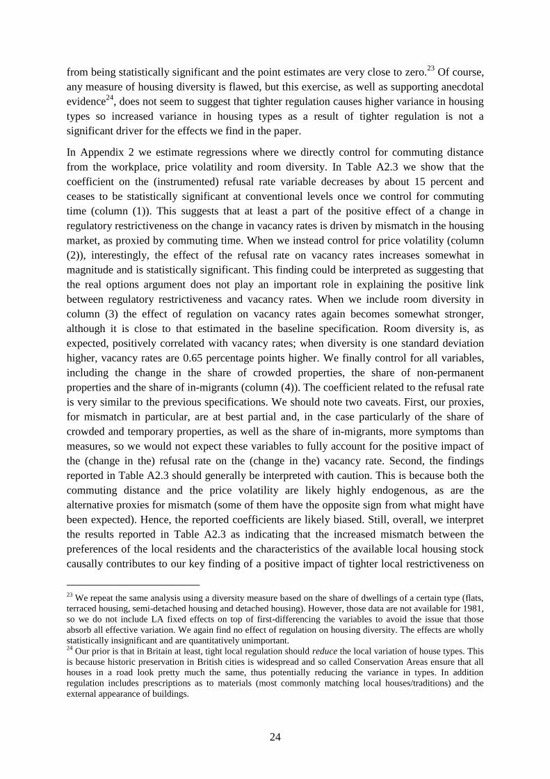
24

from being statistically significant and the point estimates are very close to zero.23

Of course,

any measure of housing diversity is flawed, but this exercise, as well as supporting anecdotal

evidence24

, does not seem to suggest that tighter regulation causes higher variance in housing

types so increased variance in housing types as a result of tighter regulation is not a

significant driver for the effects we find in the paper.

In Appendix 2 we estimate regressions where we directly control for commuting distance

from the workplace, price volatility and room diversity. In Table A2.3 we show that the

coefficient on the (instrumented) refusal rate variable decreases by about 15 percent and

ceases to be statistically significant at conventional levels once we control for commuting

time (column (1)). This suggests that at least a part of the positive effect of a change in

regulatory restrictiveness on the change in vacancy rates is driven by mismatch in the housing

market, as proxied by commuting time. When we instead control for price volatility (column

(2)), interestingly, the effect of the refusal rate on vacancy rates increases somewhat in

magnitude and is statistically significant. This finding could be interpreted as suggesting that

the real options argument does not play an important role in explaining the positive link

between regulatory restrictiveness and vacancy rates. When we include room diversity in

column (3) the effect of regulation on vacancy rates again becomes somewhat stronger,

although it is close to that estimated in the baseline specification. Room diversity is, as

expected, positively correlated with vacancy rates; when diversity is one standard deviation

higher, vacancy rates are 0.65 percentage points higher. We finally control for all variables,

including the change in the share of crowded properties, the share of non-permanent

properties and the share of in-migrants (column (4)). The coefficient related to the refusal rate

is very similar to the previous specifications. We should note two caveats. First, our proxies,

for mismatch in particular, are at best partial and, in the case particularly of the share of

crowded and temporary properties, as well as the share of in-migrants, more symptoms than

measures, so we would not expect these variables to fully account for the positive impact of

the (change in the) refusal rate on the (change in the) vacancy rate. Second, the findings

reported in Table A2.3 should generally be interpreted with caution. This is because both the

commuting distance and the price volatility are likely highly endogenous, as are the

alternative proxies for mismatch (some of them have the opposite sign from what might have

been expected). Hence, the reported coefficients are likely biased. Still, overall, we interpret

the results reported in Table A2.3 as indicating that the increased mismatch between the

preferences of the local residents and the characteristics of the available local housing stock

causally contributes to our key finding of a positive impact of tighter local restrictiveness on

23

We repeat the same analysis using a diversity measure based on the share of dwellings of a certain type (flats,

terraced housing, semi-detached housing and detached housing). However, those data are not available for 1981,

so we do not include LA fixed effects on top of first-differencing the variables to avoid the issue that those

absorb all effective variation. We again find no effect of regulation on housing diversity. The effects are wholly

statistically insignificant and are quantitatively unimportant. 24

Our prior is that in Britain at least, tight local regulation should reduce the local variation of house types. This

is because historic preservation in British cities is widespread and so called Conservation Areas ensure that all

houses in a road look pretty much the same, thus potentially reducing the variance in types. In addition

regulation includes prescriptions as to materials (most commonly matching local houses/traditions) and the

external appearance of buildings.

25

local vacancy rates. This finding is certainly plausible in the context of the extraordinarily

rigid British planning system. Whether similar effects can be observed in other countries is an

interesting question.

3.8 Sensitivity analysis

Finally, we conducted a set of robustness checks. We tested 1) the sensitivity of our choice of

polynomial in relation to changes in the share of Labour votes; 2) the possible endogeneity of

earnings; 3) whether results are driven by idiosyncratic factors associated with the Greater

London Area; 4) whether the results are sensitive to including all refusals of residential

development, not just refusals of applications for major developments; 5) whether a fixed

effects approach rather than first differencing makes any difference to the main findings; and

6) whether the change of the Census definition of vacancies in 2011 affects our findings. The

main results survive all these tests and alternative specifications essentially unchanged. The

results are set out in detail in Appendix 2.

4. Conclusions

This is the first attempt to rigorously analyse the impact of land use regulation on the spatial

and temporal variation in housing vacancy rates. It would come as no surprise to economists

to observe that in well-functioning labour markets there was unemployment. Workers search

for jobs and employers seek (better) qualified workers. Attempting to regulate unemployment

away makes no sense. Vacant houses are equivalent to unemployed workers yet, at least in

Britain, policy does try to ‘regulate’ vacant homes away by using their existence to justify

being more restrictive in the control of the supply of new homes and the structural adaptation

of existing ones.

In this paper we argue that such restrictions have two main opposing effects on housing

vacancies. The ‘opportunity cost effect’ leads to a lower vacancy rate in the more restrictive

housing markets because supply constraints lead to higher prices, and thus to higher

opportunity costs of keeping housing vacant. The ‘mismatch effect’, however, implies higher

vacancy rates in the more restrictive housing markets because households will find it more

difficult to match their preferences to the characteristics of the local housing supply given

their budget constraints. So search becomes more prolonged and costly and households

choose to search for properties further afield and commute longer.

We do indeed confirm that there is a simple negative correlation between local planning

restrictiveness and local housing vacancies. Superficially this appears to support the planners’

‘common sense’ that the existence of empty houses means they can – even should – plan to

be more restrictive in supply. This unconditional correlation, however, is the result of a form

of joint causation. When we effectively control for unobserved characteristics at the local

level by using first differencing, the negative correlation turns positive. When we further

control for local linear trends, for other potential explanatory variables and account for the

endogeneity of local regulatory restrictiveness, the causal effect of restrictiveness on vacancy

rates is firmly positive, statistically significant and economically substantial.

26

Our empirical analysis does not fully unpack the box of explanations. It is a reduced form

telling us what the net impact of increased planning restrictiveness is on housing vacancies. If

an LA becomes more restrictive, signalled by an increase in the rate of refusal of residential

development proposals, then all else equal, vacancy rates increase in that LA. We also

provide direct evidence that mismatch may be an important reason for higher vacancy rates in

more restrictive housing markets: The more restrictive in planning terms a local jurisdiction

is, the longer is the average commuting distance of workers within it. We subject these

findings to an extensive range of sensitivity analyses. They survive remarkably unaltered.

Welfare implications in markets with search frictions are not easy to derive. This is because

in such a second best world, households may search less or more than would be welfare

optimal (Koster and Van Ommeren, 2017). This paper does not set out to assess the net

welfare impact of tightening the supply of housing. However, because regulatory constraints

seem to worsen matching for households, the effect of tighter restrictions on vacancies and

commute times unequivocally generates a welfare cost.

It is the mismatch between the preferences of households and the housing stock on offer that

leads, other things equal, to higher vacancy rates in the more regulated – typically more

desirable – places. This is not to say that tighter regulatory constraints in some places

necessarily increase vacancy rates at the aggregate level (for the whole country). However,

even if on aggregate vacancy rates were unaffected by regulatory restrictiveness, such

constraints will still likely cause a significant welfare loss. This is because too much housing

stays empty in the most regulated, most desirable and, by implication, most productive places

with the strongest demand and highest valuations for living space. So people are induced to

commute further, while living in the “wrong” places.

There are important implications for policy, particularly for the UK because of its

extraordinarily restrictive planning system. Crucially planners should not allocate less land

for development on the grounds that there are empty houses. Some vacancies are integral to

the well-functioning of any market and, as our results show, trying to ‘regulate housing

vacancies away’ is counterproductive. There is moreover a nice irony for advocates of the

‘compact city’. The most common policy to attempt to implement this ideal is to impose

growth boundaries (make land scarcer) and be more restrictive to adaptations of the existing

stock or – in the US – make it more difficult to obtain zoning ordinance waivers. In summary

aiming for a compact city makes planning policy more restrictive. Our results show this will

have exactly the opposite to the intended effect because average commuting distances will

lengthen as residents search further afield for housing they can afford and matches their

preferences.

27

References

Angrist, J.D. and Pischke, J.D. (2009). Mostly Harmless Econometrics: An Empiricists

Companion. Princeton: Princeton University Press.

Bartik, T. (1991). Who Benefits from State and Local Economic Development Policies?

Kalamazoo, MI: W.E. Upjohn Institute for Employment Research.

Bertrand, M. and Kramarz, F. (2002). Does Entry Regulation Hinder Job Creation? Evidence

from the French Retail Industry. Quarterly Journal of Economics 117: 1369-1413.

Cheshire, P.C. and Sheppard, S. (1998). Estimating the Demand for Housing, Land and

Neighbourhood Characteristics. Oxford Bulletin of Economics and Statistics 60(3), 357-

382.

Cheshire, P.C. and Sheppard, S. (2002). Welfare Economics of Land Use Regulation Journal

of Urban Economics, 52, 242-69.

Cheshire, P.C. and Sheppard, S. (2005). The Introduction of Price Signals into Land Use

Planning Decision-making: a proposal. Urban Studies 42: 647-663.

Cheshire, P.C., C.A.L. Hilber and I. Kaplanis (2015). “Land use regulation and

productivity—land matters: evidence from a supermarket chain,” Journal of Economic

Geography 15: 43-73.

Davidoff, T. (2016). “Supply Constraints are not Valid Instrumental Variables for Home

Prices because they are Correlated with Many Demand Factors,” Critical Finance Review

5, 177-206.

Deng, Y., Gabriel, S.A., Nothaft, F.E. (2003). Duration of Residence in the Rental Housing

Market. Journal of Real Estate Finance and Economics 26(2-3): 267-285.

Department of Transport (2013). Vehicle Statistics. Statistics Information on Licensed and

Unlicensed Vehicles, and MOT Testing. https://www.gov.uk/government/collections/

vehicles-statistics.

Ferreira, F. and Gyourko, J. (2009). Do Political Parties Matter? Evidence from U.S. cities.

Quarterly Journal of Economics, Vol. 124(1): 399-422.

Gabriel, S.A. and Nothaft, F.E. (1988). Rental Housing Markets and the Natural Vacancy

Rate. Journal of the American Real Estate and Urban Economics Association [now Real

Estate Economics] 16(4): 419-429.

Gabriel, S.A. and Nothaft, F.E. (2001). Rental Housing Markets, Incidence and Duration of

Vacancy, and the Natural Vacancy Rate. Journal of Urban Economics 49: 121-149.

Glaeser, E.L. and Gyourko, J. (2003). The Impact of Building Restrictions on Housing

Affordability. Economic Policy Review 9: 21-39.

Glaeser, E.L., Gyourko, J. and Saks, R.E. (2005a). Why Have Housing Prices Gone Up?

American Economic Review 95(2): 329-333.

Glaeser, E.L., Gyourko, J. and Saks, R.E. (2005b). Why is Manhattan so Expensive?

Regulation and the Rise in Housing Prices. Journal of Law and Economics 48: 331-369.

28

Glaeser, E.L., Gyourko, J. and Saks, R.E. (2006). Urban growth and housing supply. Journal

of Economic Geography 6(1): 71–89.

Grenadier, S.R. (1995). The persistence of real estate cycles. Journal of Real Estate Finance

and Economics, 10: 95-121.

Grenadier, S.R. (1996). The Strategic Exercise of Options: Development Cascades and

Overbuilding in Real Estate Markets. Journal of Finance 51(5): 1653-1679.

Government Office for the East Midlands (2005). Regional Spatial Strategy for the East

Midlands (RSS8).

Ha, S. and Hilber, C.A.L. (2013). Do Long Distance Moves Discourage Homeownership?

Evidence from England. SERC Discussion Paper No. 141.

Han, L., Strange, W.C. (2015). The Microstructure of Housing Markets: Search, Bargaining,

and Brokerage. In: Duranton, G., Henderson, J.V., Strange, W.C. (eds.). Handbook of

Regional and Urban Economics, Volume 5. Amsterdam: Elsevier.

Hilber, C.A.L. and Robert-Nicoud, F. (2013). On the Origins of Land Use Regulations:

Theory and Evidence from US Metro Areas. Journal of Urban Economics 75(1): 29-43.

Hilber, C.A.L. and Vermeulen, W. (2016). The Impact of Supply Constraints on House Prices

in England. Economic Journal 126(591), 358-405.

Hilber, C.A.L., T. Lyytikäinen and W. Vermeulen (2011). Capitalization of Central

Government Grants into Local House Prices: Panel Data Evidence from England.

Regional Science and Urban Economics 41(4), 394-406.

Ihlanfeldt, K.R. (2007). The Effect of Land Use Regulation on Housing and Land Prices.

Journal of Urban Economics 61: 420-435.

Koster, H.R.A. and Van Ommeren, J.N. (2017). On Housing Search Frictions: Hedonic Price

Models, Optimal Search and Welfare. Mimeo, Vrije Universiteit Amsterdam.

McDonald, R. and Siegel, D. (1986). The Value of Waiting to Invest. Quarterly Journal of

Economics 101: 707-727.

Merlo, A., and Ortalo-Magné, F. (2004). Bargaining over Residential Real Estate: Evidence

from England. Journal of Urban Economics 56(2): 192–216.

Molloy, R. (2016). Long-Term Vacant Housing in the United States. Regional Science and

Urban Economics 59: 118-129.

Mortensen, D.T. and Pissarides, C.A. (1994). Job Creation and Job Destruction in the Theory

of Unemployment. Review of Economic Studies 61(3): 397-415.

Mulalic, I., Van Ommeren, J. N., and Pilegaard, N. (2014) Wages and Commuting: Quasi-

natural Experiments’ Evidence from Firms that Relocate. Economic Journal 124: 1086-

1105.

Pawson, H. and Kintrea, K. (2002). Part of the Problem or part of the Solution? Social

Housing Allocation Policies and Social Exclusion in Britain. Journal of Social Policy

31(4): 643-667.

29

Pissarides, C.A. (1985). Short-Run Equilibrium Dynamics of Unemployment, Vacancies, and

Real Wages. American Economic Review 75(4): 676-690.

Pissarides, C.A. (1994). Search Unemployment with On-the-job Search. Review of Economic

Studies 61(3): 457-475.

Quigley, J.M., Raphael, S. (2005). Regulation and the High Cost of Housing in California.

American Economic Review 95(2): 323-328.

Rallings, C. and Thrasher, M. (eds.) (2004). Local Elections in Britain: A Statistical Digest.

Local Government Chronicle Elections Centre, Plymouth.

Rosen, K.T., Smith, L.B. (1983). The Price-Adjustment Process for Rental Housing and the

Natural Vacancy Rate. American Economic Review 73(4): 779-786.

Sadun, R. (2015) “Does Planning Regulation Protect Independent Retailers?,” Review of

Economics and Statistics 97: 983-1001.

Saks, R.E. (2008). Job Creation and Housing Construction: Constraints on Metropolitan Area

Employment Growth. Journal of Urban Economics 64(1): 178–95.

Wall, D. (1998). The Development of a Land Registry-based National House Price Index.

Economic Trends 541(12): 57–61.

Wheaton, W.C. (1990). Vacancy, Search, and Prices in a Housing Market Matching Model.

Journal of Political Economy 98(6): 1270-1292.

30

TABLES

TABLE 1

Descriptive statistics (repeated cross-section)

Mean Std. Dev. Min Max

Vacancy rate (in %) 3.886 1.340 0 12.06

Refusal rate, t-2 (in %) 27.43 14.63 0 78.57

House price (in £) 141,665 91,729 43,804 1.277e+06

Male weekly earnings (in £) 545.7 147.3 258.3 1,793

Share owner-occupied housing (in %) 66.86 11.22 4.611 89.52

Share council housing (in %) 16.09 11.34 0.416 81.96

Share age 30-65 (in %) 44.87 2.783 36.42 51.62

Share age >65 (in %) 16.42 3.642 6.128 31.36

Share unemployed (in %) 6.516 2.960 2.042 22.40

Share highly educated (in %) 13.74 11.39 0.244 53.57

Share permanent illness (in %) 3.478 1.878 0.745 12.15

Predicted employment (‘Bartik instrument’)† 57,913 47,674 9,832 474,473

Share Labour seats, t-2, (in %) 30.87 26.86 0 99.17

Share Labour voters, local elections (in %) 31.49 16.76 0 76.95

Share Labour voters, general election (in %) 29.53 15.21 2.426 75.25

Mean commuting distance from workplace (in km) 6.853 3.465 2.141 18.66

Share crowded properties (in %) 1.952 1.567 0.399 14.99

Share non-permanent properties (in %) 57.23 59.05 0.670 586.2

Share migrants (in %) 10.84 3.328 0.466 36.51

Coefficient of variation house prices, t+3 0.104 0.0745 0.00755 0.460

Coefficient of variation earnings, t+3 0.0755 0.0400 0.00685 0.674

Room diversity 4.589 0.419 3.496 6.259

Unitary authority 0.123 0.328 0 1

Net expenditures on education (in £ per head) 436.9 278.0 17.67 1,643

Net expenditures on social services (in £ per head) 169.4 147.9 17.32 741.8

Net expenditures on highways (in £ per head) 38.96 18.99 -72.89 119.2

Net local expenditures on housing services (in £ per head) 12.81 24.02 -3.605 210.2

Net local expenditures on planning (in £ per head) 12.15 16.16 -29.26 308.1

Total local net expenditures (in £ per head) 373.0 554.6 15.04 3,054

Notes: The number of observations is 1,400, as we have 4 observations for 350 local authorities. t-2 denotes that we

include applications up to two years preceding and including the year of observation, t+4 denotes that we include data up

to four years after and including the year of observation. † Measure is based on 1971 local industry composition.

31

TABLE 2

Baseline results – second stage

(Dependent variable: Δ Vacancy rate)

(1) (2) (3) (4) (5) (6) (7)

OLS OLS OLS 2SLS 2SLS 2SLS 2SLS

Δ Refusal rate, t-2 0.0434 0.101* 0.0801+ 0.820** 0.855** 0.840** 0.895*

(0.0382) (0.0532) (0.0501) (0.417) (0.405) (0.354) (0.530)

Δ Earnings (log) 0.373 -0.0701 -0.125

(0.677) (0.692) (0.719)

Δ Share owner-occupied housing -0.129 -0.262 -0.321

(0.356) (0.369) (0.418)

Δ Share council housing 0.736*** 0.655*** 0.631***

(0.235) (0.219) (0.233)

Δ Share age 30-65 -0.0989 0.0550 0.0754

(0.208) (0.202) (0.211)

Δ Share age >65 1.281*** 1.432*** 1.362***

(0.317) (0.311) (0.319)

Δ Share unemployed 0.368*** 0.270** 0.276**

(0.138) (0.114) (0.136)

Δ Share highly educated -0.493** -0.581*** -0.617***

(0.191) (0.189) (0.214)

Δ Share permanent illness 0.192** 0.151 0.123

(0.0972) (0.0934) (0.0985)

Year fixed effects (3) Yes Yes Yes Yes Yes Yes Yes

Local authority fixed effects (350) No Yes Yes No Yes Yes Yes

Δ Share Labour voters local elections Ω( ∙ ) No No No No No No Yes

Observations 1,050 1,050 1,050 1,050 1,050 1,050 1,050

R-squared 0.373 0.488 0.559

Kleibergen-Paap F-statistic 18.52 17.49 19.01 8.151 Notes: All independent variables (except for earnings) are standardised with mean zero and unit standard deviation. Bold indicates instrumented. In Models (4)-(7), the

instrument for Δ Refusal rate is Δ Share of Labour seats in the LA. Ω( ∙ ) is approximated by a fifth-order polynomial of share Labour voters in local elections. Standard

errors in parentheses are clustered at the LA level. *** p<0.01, ** p<0.05, * p<0.10, + p<0.15.

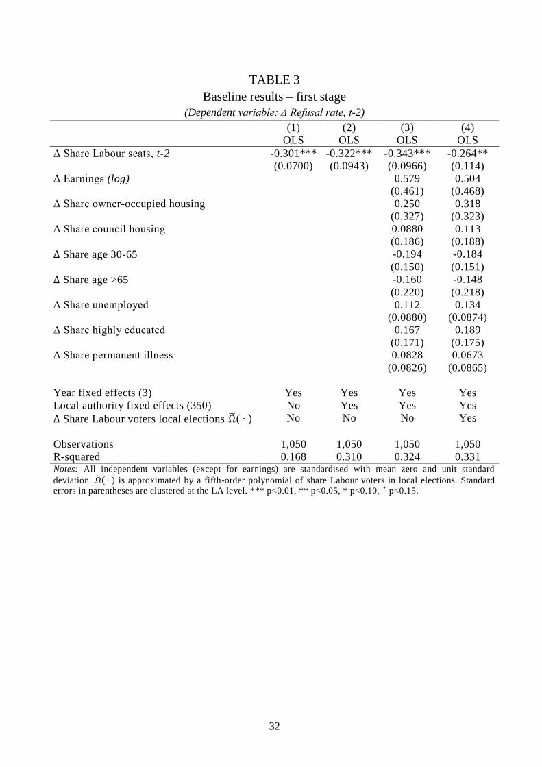
32

TABLE 3

Baseline results – first stage

(Dependent variable: Δ Refusal rate, t-2)

(1) (2) (3) (4)

OLS OLS OLS OLS

Δ Share Labour seats, t-2 -0.301*** -0.322*** -0.343*** -0.264**

(0.0700) (0.0943) (0.0966) (0.114)

Δ Earnings (log) 0.579 0.504

(0.461) (0.468)

Δ Share owner-occupied housing 0.250 0.318

(0.327) (0.323)

Δ Share council housing 0.0880 0.113

(0.186) (0.188)

Δ Share age 30-65 -0.194 -0.184

(0.150) (0.151)

Δ Share age >65 -0.160 -0.148

(0.220) (0.218)

Δ Share unemployed 0.112 0.134

(0.0880) (0.0874)

Δ Share highly educated 0.167 0.189

(0.171) (0.175)

Δ Share permanent illness 0.0828 0.0673

(0.0826) (0.0865)

Year fixed effects (3) Yes Yes Yes Yes

Local authority fixed effects (350) No Yes Yes Yes

Δ Share Labour voters local elections Ω̃( ∙ ) No No No Yes

Observations 1,050 1,050 1,050 1,050

R-squared 0.168 0.310 0.324 0.331 Notes: All independent variables (except for earnings) are standardised with mean zero and unit standard

deviation. Ω̃( ∙ ) is approximated by a fifth-order polynomial of share Labour voters in local elections. Standard

errors in parentheses are clustered at the LA level. *** p<0.01, ** p<0.05, * p<0.10, + p<0.15.

33

TABLE 4

Baseline results – second stage

(Dependent variable: Δ Commuting distance from workplace (log))

(1) (2) (3) (4) (5) (6) (7)

OLS OLS OLS 2SLS 2SLS 2SLS 2SLS

Δ Refusal rate, t-2 -0.00274 0.00341 0.00106 0.0847*** 0.0584** 0.0594** 0.0608+

(0.00283) (0.00400) (0.00384) (0.0321) (0.0296) (0.0274) (0.0407)

Δ Earnings (log) 0.179*** 0.145*** 0.139**

(0.0567) (0.0548) (0.0548)

Δ Share owner-occupied housing 0.0551* 0.0449+ 0.0420

(0.0286) (0.0296) (0.0328)

Δ Share council housing -0.00297 -0.00916 -0.0100

(0.0177) (0.0158) (0.0163)

Δ Share age 30-65 -0.0216+ -0.00982 -0.00803

(0.0131) (0.0145) (0.0153)

Δ Share age >65 0.0168 0.0285 0.0225

(0.0319) (0.0312) (0.0319)

Δ Share unemployed 0.0181** 0.0106 0.0120

(0.00755) (0.00781) (0.00927)

Δ Share highly educated 0.00129 -0.00544 -0.00902

(0.0123) (0.0122) (0.0139)

Δ Share permanent illness -0.0245*** -0.0277*** -0.0306***

(0.00915) (0.00882) (0.00912)

Year fixed effects (3) Yes Yes Yes Yes Yes Yes Yes

Local authority fixed effects (350) No Yes Yes No Yes Yes Yes

Δ Share Labour voters local elections Ω( ∙ ) No No No No No No Yes

Observations 1,050 1,050 1,050 1,050 1,050 1,050 1,050

R-squared 0.373 0.913 0.559

Kleibergen-Paap F-statistic 18.52 17.49 19.01 8.151 Notes: All independent variables (except for earnings) are standardised with mean zero and unit standard deviation. Bold indicates instrumented. In Models (4)-(7), the

instrument for Δ Refusal rate is Δ Share of Labour seats in the LA. Ω( ∙ ) is approximated by a fifth-order polynomial of share Labour voters in local elections. Standard

errors in parentheses are clustered at the LA level. *** p<0.01, ** p<0.05, * p<0.10, + p<0.15.

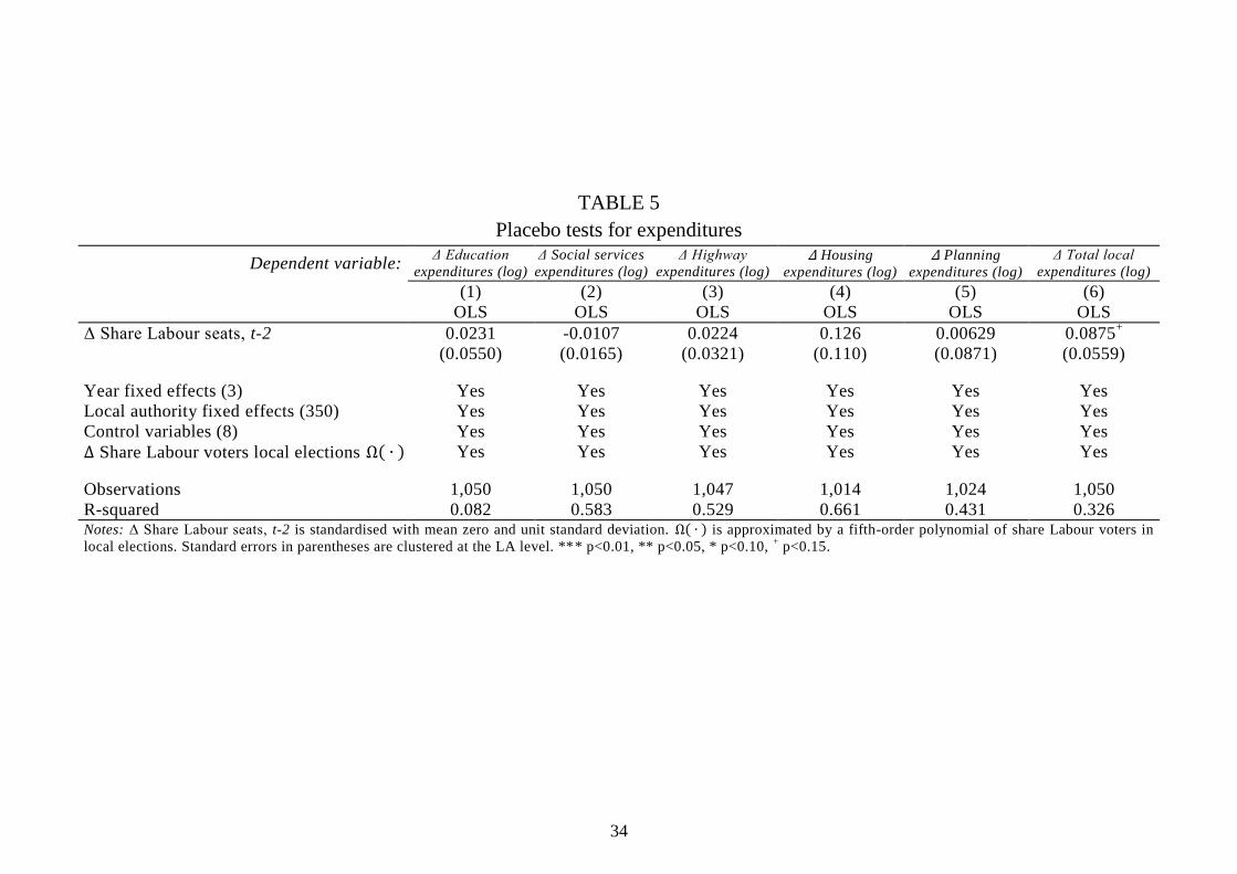
34

TABLE 5

Placebo tests for expenditures

Dependent variable: Δ Education

expenditures (log)

Δ Social services

expenditures (log)

Δ Highway

expenditures (log) Δ Housing

expenditures (log)

Δ Planning

expenditures (log)

Δ Total local

expenditures (log)

(1) (2) (3) (4) (5) (6)

OLS OLS OLS OLS OLS OLS

Δ Share Labour seats, t-2 0.0231 -0.0107 0.0224 0.126 0.00629 0.0875+

(0.0550) (0.0165) (0.0321) (0.110) (0.0871) (0.0559)

Year fixed effects (3) Yes Yes Yes Yes Yes Yes

Local authority fixed effects (350) Yes Yes Yes Yes Yes Yes

Control variables (8) Yes Yes Yes Yes Yes Yes

Δ Share Labour voters local elections Ω( ∙ ) Yes Yes Yes Yes Yes Yes

Observations 1,050 1,050 1,047 1,014 1,024 1,050

R-squared 0.082 0.583 0.529 0.661 0.431 0.326 Notes: Δ Share Labour seats, t-2 is standardised with mean zero and unit standard deviation. Ω( ∙ ) is approximated by a fifth-order polynomial of share Labour voters in

local elections. Standard errors in parentheses are clustered at the LA level. *** p<0.01, ** p<0.05, * p<0.10, + p<0.15.

35

TABLE 6

Results for Unitary Authorities and other LAs

PANEL A – (Dependent variable: (1) (2) (3) (4)

Δ Refusal rate, t-2) OLS OLS OLS OLS

Δ Share Labour seats, t-2 × -0.326*** -0.352*** -0.365*** -0.291**

Other local authority (0.0743) (0.0998) (0.102) (0.120)

Δ Share Labour seats, t-2 × -0.144 -0.121 -0.187 -0.153

Unitary authority (0.162) (0.210) (0.205) (0.215)

Year fixed effects (3) Yes Yes Yes Yes

Local authority FEs (350) No Yes Yes Yes

Control variables included (8) No No Yes Yes

Δ Share Labour voters local elections Ω̃( ∙ ) No No No Yes

Observations 1,050 1,050 1,050 1,050

R-squared 0.169 0.311 0.325 0.326

PANEL B – (Dependent variable: (1) (2) (3) (4)

Δ Vacancy rate) 2SLS 2SLS 2SLS 2SLS

Δ Refusal rate, t-2 0.915** 0.906** 0.855** 0.935*

(0.423) (0.399) (0.359) (0.541)

Δ Share Labour seats, t-2 × 0.209 0.126 0.0421 0.0786

Unitary authority (0.207) (0.216) (0.196) (0.212)

Year fixed effects (3) Yes Yes Yes Yes

Local authority FEs (350) No Yes Yes Yes

Control variables included (8) No No Yes Yes

Δ Share Labour voters local elections Ω̃( ∙ ) No No No Yes

Observations 1,050 1,050 1,050 1,050

Kleibergen-Paap F-statistic 19.31 18.65 19.25 8.354

PANEL C – (Dependent variable: (1) (2) (3) (4)

Δ Commuting distance from workplace (log)) 2SLS 2SLS 2SLS 2SLS

Δ Refusal rate, t-2 0.102*** 0.0735** 0.0664** 0.0720*

(0.0342) (0.0307) (0.0284) (0.0432)

Δ Share Labour seats, t-2 × 0.0371** 0.0377*** 0.0195 0.0217+

Unitary authority (0.0164) (0.0139) (0.0136) (0.0141)

Year fixed effects (3) Yes Yes Yes Yes

Local authority FEs (350) No Yes Yes Yes

Control variables included (8) No No Yes Yes

Δ Share Labour voters local elections Ω̃( ∙ ) No No No Yes

Observations 1,050 1,050 1,050 1,050

Kleibergen-Paap F-statistic 19.31 18.65 19.25 8.354 Notes: Bold indicates instrumented. The instrument is Δ Share Labour seats, t-2 × Other Local authority. All

independent variables (except for earnings) are standardised with mean zero and unit standard deviation. Ω( ∙ ) is

approximated by a fifth-order polynomial of share Labour voters in local elections. Standard errors in parentheses a re

clustered at the LA level. *** p<0.01, ** p<0.05, * p<0.10, + p<0.15.

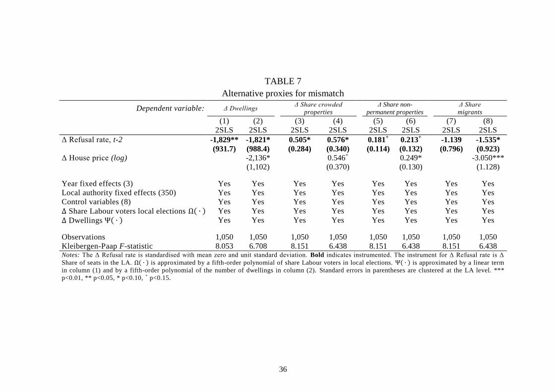
36

TABLE 7

Alternative proxies for mismatch

Dependent variable: Δ Dwellings Δ Share crowded

properties

Δ Share non-

permanent properties Δ Share

migrants

(1) (2) (3) (4) (5) (6) (7) (8)

2SLS 2SLS 2SLS 2SLS 2SLS 2SLS 2SLS 2SLS

Δ Refusal rate, t-2 -1,829** -1,821* 0.505* 0.576* 0.181+ 0.213

+ -1.139 -1.535*

(931.7) (988.4) (0.284) (0.340) (0.114) (0.132) (0.796) (0.923)

Δ House price (log) -2,136* 0.546+ 0.249* -3.050***

(1,102) (0.370) (0.130) (1.128)

Year fixed effects (3) Yes Yes Yes Yes Yes Yes Yes Yes

Local authority fixed effects (350) Yes Yes Yes Yes Yes Yes Yes Yes

Control variables (8) Yes Yes Yes Yes Yes Yes Yes Yes

Δ Share Labour voters local elections Ω( ∙ ) Yes Yes Yes Yes Yes Yes Yes Yes

Δ Dwellings Ψ( ∙ ) Yes Yes Yes Yes Yes Yes Yes Yes

Observations 1,050 1,050 1,050 1,050 1,050 1,050 1,050 1,050

Kleibergen-Paap F-statistic 8.053 6.708 8.151 6.438 8.151 6.438 8.151 6.438 Notes: The Δ Refusal rate is standardised with mean zero and unit standard deviation. Bold indicates instrumented. The instrument for Δ Refusal rate is Δ

Share of seats in the LA. Ω( ∙ ) is approximated by a fifth-order polynomial of share Labour voters in local elections. Ψ( ∙ ) is approximated by a linear term

in column (1) and by a fifth-order polynomial of the number of dwellings in column (2). Standard errors in parentheses are clustered at the LA level. ***

p<0.01, ** p<0.05, * p<0.10, + p<0.15.

37

TABLE 8

Real options, housing diversity and regulatory restrictiveness

PANEL A – Second stage (Dependent variable: (1) (2) (3) (4) (5) (6) (7)

Δ Coefficient of variation of house prices, t+3) OLS OLS OLS 2SLS 2SLS 2SLS 2SLS

Δ Refusal rate, t-2 0.00501 0.00784 0.00857 -0.0892* -0.119** -0.0726* -0.117*

(0.00453) (0.00743) (0.00659) (0.0480) (0.0605) (0.0434) (0.0680)

Δ Refusal rate, t-2 × Coefficient of variation -0.0375 -0.0725 -0.0758 0.804* 1.166** 0.693* 0.812*

of earnings, t+3 (0.0606) (0.101) (0.0858) (0.411) (0.570) (0.368) (0.468)

Year fixed effects (3) Yes Yes Yes Yes Yes Yes Yes

Local authority fixed effects (350) No Yes Yes No Yes Yes Yes

Control variables included (8) No No Yes No No Yes Yes

Δ Share Labour voters local elections Ω( ∙ ) No No No No No No Yes

Observations 1,050 1,050 1,050 1,050 1,050 1,050 1,050

R-squared 0.808 0.826 0.864

Kleibergen-Paap F-statistic 5.212 4.573 5.419 2.893

PANEL B – Second stage (Dependent variable: (1) (2) (3) (4) (5) (6) (7)

Δ Room diversity) OLS OLS OLS 2SLS 2SLS 2SLS 2SLS

Δ Refusal rate, t-2 -0.00186 -0.00410 -0.000875 0.0900* 0.0294 0.00427 0.0180

(0.00465) (0.00549) (0.00492) (0.0485) (0.0339) (0.0276) (0.0399)

Year fixed effects (3) Yes Yes Yes Yes Yes Yes Yes

Local authority fixed effects (350) No Yes Yes No Yes Yes Yes

Control variables included (8) No No Yes No No Yes Yes

Δ Share Labour voters local elections Ω( ∙ ) No No No No No No Yes

Observations 1,050 1,050 1,050 1,050 1,050 1,050 1,050

R-squared 0.160 0.653 0.726

Kleibergen-Paap F-statistic 18.52 17.49 19.01 8.151 Notes: All independent variables (except for earnings) are standardised with mean zero and unit standard deviation. Bold indicates instrumented. In Models (4)-(7),

instruments for Δ Refusal rate and Δ Refusal rate × Coefficient of variation of earnings are Δ Sha re of Labour seats and Δ Share of Labour seats × Coefficient of variation

of earnings. Ω( ∙ ) is approximated by a fifth-order polynomial of share Labour voters. Standard errors in parentheses are clustered at the LA level. *** p<0.01, ** p<0.05, *

p<0.10, + p<0.15.

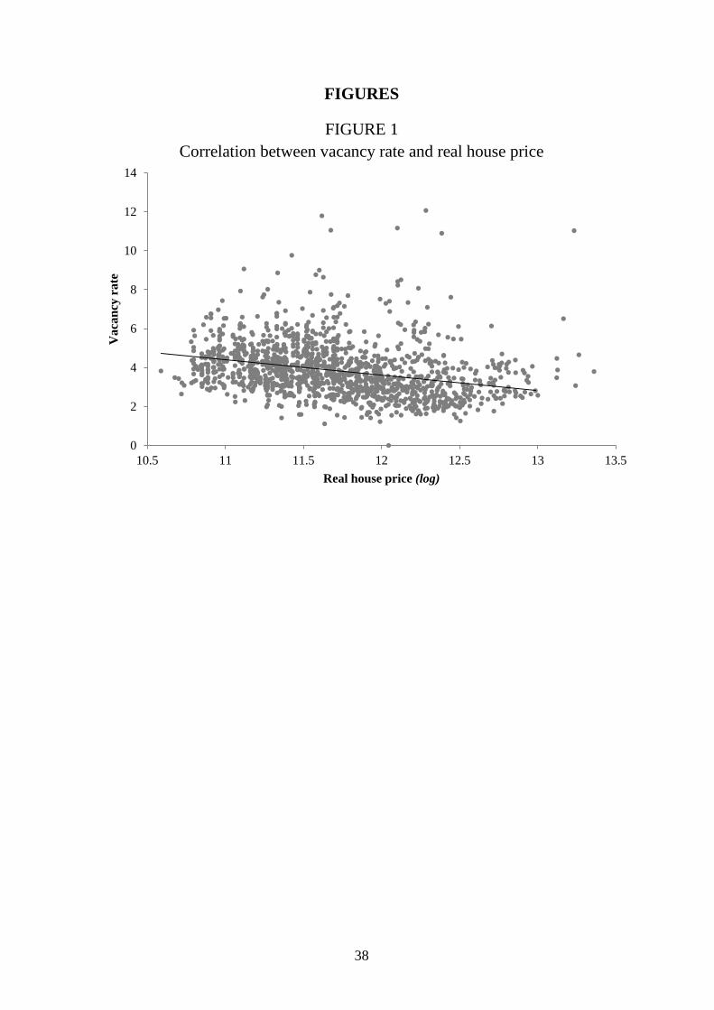
38

FIGURES

FIGURE 1

Correlation between vacancy rate and real house price

0

2

4

6

8

10

12

14

10.5 11 11.5 12 12.5 13 13.5

Va

can

cy r

ate

Real house price (log)

39

FIGURE 2

Vacancy rate across England

40

FIGURE 3

Housing supply restrictions across England (refusal rate by LA)

41

FIGURE 4

Correlation between Labour votes and Labour seats

FIGURE 5

Cross-sectional relationship between refusal rate and vacancy rate

0.0

0.1

0.2

0.3

0.4

0.5

0.6

0.7

0.8

0.9

1.0

0.0 0.1 0.2 0.3 0.4 0.5 0.6 0.7 0.8 0.9 1.0

Sh

are

La

bo

ur

sea

ts

Share Labour votes

0

1

2

3

4

5

6

7

8

9

10

0 10 20 30 40 50 60

Aver

age

vaca

ncy

rate

1981

-2011

Average major refusal rate 1981-2011

42

APPENDICES

APPENDIX 1: Election data

The local election data are obtained from three different sources. The first source is the

British Local Election Database, which is compiled by Rallings and Thrasher (2004). They

have combined different data sources on local election outcomes from 1889 to 2003. From

1973, the data contain the universe of local election outcomes. The data are available on a

ward level and display for every election the number of candidates, the number of votes per

candidate and the number of vacant seats. Councillors that received the most votes will be

elected. It is important to note that the share of votes for each party is therefore not perfectly

correlated to the assigned number of seats. Based on the number of votes, we determine

which candidate is elected as a councillor. The British Local Election Database only provides

information on the election results, and not on the current composition of the LA. The

problem is that for many local authorities, there are yearly or two-yearly elections of which

33 percent of the seats are replaced. To estimate the composition of the local council, we use

the fact that the full electoral term for councillors is usually four years. However, sometimes

elections replace the complete council despite the fact that councillors did not complete the

electoral term, for example due to changes in boundaries of local authorities. To account for

this, we consider full elections as elections where at least 75 percent of the seats are replaced.

The second data source for local election results is the local election handbooks from 1999 to

2008 (see Hilber et al., 2011). These data provide the number of council seats for each local

authority in each year. We measure the correlation of the shares of seats of different parties

(Labour, Conservatives, Liberal Democrats, Other) between the British Local Election

Database and the latter database for the overlapping years. This is always above 0.95. For the

overlapping years, we take the average of shares in seats in both datasets. For 2006-2011, we

obtain information on Labour votes (rather than seats) from the Local Elections Archive

Project (LEAP). For 55 LAs, we do not have information available for the most recent

election in 2011. We then use information on Labour vote shares for the 2007 elections. We

made sure that excluding these 55 LA lead to essentially the same results. The final dataset is

from the BBC with the outcomes of local council elections for 2009, 2010 and 2011 to

complement the LEAP when necessary.

We also use outcomes of general elections to control for demographic changes and general

trends in political preferences. We have data of election results for 1983, 1987, 1991, 1997,

2001, 2005 and 2010 obtained from Electoral Calculus. We match each year to the previous

election, except for 1981, which is matched to 1983. The results are available at the

parliamentary constituency level, which are almost always smaller than LAs. Using

geographical information systems, we calculate the geographical overlap of each

constituency with each LA and assign the votes accordingly.

In Figure 4 we provide a scatterplot of the share of Labour votes and the share of Labour

seats from 1978-2011 for each year and local authority. Not surprisingly there is a strong

positive correlation between seats and votes. However, below a vote share of one third, votes

translate into a less than proportional number of seats (denoted by the dashed line). In a

43

number of cases votes did not even translate into any seats at all. Furthermore, because of the

‘first-past-the-post feature of the system’, above a vote share of one third, votes lead to a

more than proportional number of seats. When having more than 70 percent of the votes

usually implies that all seats are assigned to the Labour party.

Table A1.1 shows correlations for the election variables of the Labour party in our data: The

correlation between the share of Labour council seats and the share of Labour votes is high

(0.87). The correlation with the general election vote share is somewhat lower, but still

reasonable high (0.67). If we look at the correlation between the changes, these are lower

(respectively 0.57 and 0.48).

TABLE A1.1

Correlations between election variables

Share Labour

seats

Share Labour

votes

Share Labour

votes gen. elec.

Share Labour seats, t-2 1.0000

Share Labour votes 0.8761 1.0000

Share Labour votes general elections 0.6901 0.6060 1.0000

Δ Share

Labour seats

Δ Share

Labour votes

Δ Share Labour

votes gen. elec.

Δ Share Labour seats, t-2 1.0000

Δ Share Labour votes 0.5706 1.0000

Δ Share Labour votes general elections 0.4474 0.3834 1.0000

44

APPENDIX 2: Sensitivity analysis

To begin with, we re-estimate the preferred specification (column (7), Table 2), but include

LA expenditure by category, one by one, as additional controls (columns (1) to (5)). In

column (6) we instead include total local expenditures as an additional control. We report the

results for vacancy rates in Table A2.1 below. The coefficients unequivocally indicate that

the impact of the refusal rate on vacancy rates is unaffected, even when we control for total

local expenditures or for each category of expenditure individually. Planning expenses seem

to have some direct negative impact on vacancy rates (column (5)), so more planning

expenses lead to lower vacancy rates. In column (6) we show that, even when the share of

Labour seats might have a positive effect on total local expenditures (see Table 5), it seems

that local expenditures do not have a direct impact on vacancy rates. Hence, this provides

additional evidence that the exclusion restriction holds.

We also do a similar exercise but take the change in the log of commuting time as dependent

variable. The results reported in Table A2.2 suggest that the effect of regulation on

commuting distances cannot be explained by differences in expenditures on education, social

services, highways, or planning. Column (4) shows that when controlling for housing

expenditures the effect of regulation becomes statistically insignificant (p-value = 0.222). We

do, however, not worry too much because the impact of housing expenditures is highly

insignificant and the point estimate is very similar to the baseline estimate. On the other hand,

column (6) suggests that the effect of commuting is even somewhat stronger, despite the

effect that the total LA expenditures have a positive and statistically significant effect on

commuting distance.

Next, we include commuting distance, price volatility and room diversity as additional

controls in the regression of vacancy rates on the refusal rate. Table A2.3 reports the results,

where column (7) in Table 2 is the corresponding specification. In column (1) of Table A2.3

we show that commuting distance is positively associated with higher vacancy rates. A one

kilometre increase in the average commuting distance is associated with an increase in the

vacancy rate of about 2 percentage points. We do not interpret this as a strictly causal effect,

but the sign is in line with our expectations. The effect of restrictiveness is about 15 percent

lower compared to the baseline specification. The effect is now statistically significantly

different from zero only at the 13 percent level (p-value = 0.131). Commuting distance is a

crude proxy for mismatch in the housing market, which may explain why the effect of

interest is only somewhat smaller. In column (2) we include the coefficient of variation of

prices in the year of observation and the three years subsequent to the year of observation.

The coefficient is positive and highly statistically significant. Interestingly, the coefficient on

regulatory restrictiveness is now somewhat higher compared to the baseline specification.

Column (3) investigates the effect of regulation on vacancy rates again, while controlling for

room diversity. The effect of the refusal rate becomes somewhat stronger, although it is close

to the baseline specification. Room diversity is, as expected, positively correlated to vacancy

rates. In column (4), Table A2.3, we control for all variables, including the change in the

share of crowded properties, the share of non-permanent homes and the share migrants. The

coefficient related to the refusal rate is very similar to the previous specifications.

45

Recall that in our preferred specification (column (7) of Table 2), we included a fifth-order

polynomial of changes in the share Labour votes in each LA. This is to isolate the impact of

potentially unobserved demographic and socio-economic variables, which may be reflected

in voting behaviour, from local political power. However, the choice of the order of

polynomial is somewhat arbitrary. Table A2.4 investigates the robustness of the results to this

choice. Panel A reports second-stage results, whereas Panel B reports the corresponding first-

stage results. In column (1) of Panel A we include only a linear term of change in the share

Labour votes in local elections as a control. Changes in the share of Labour votes do not have

a direct effect on changes in vacancy rates. The coefficient on the change in the refusal rate

variable is statistically significant at the 11 percent level. When we include a third or fourth

order polynomial of change in share Labour votes, the coefficient on the change in the refusal

rate variable becomes slightly higher and statistically significant at the 10 percent level. In

column (5) we include a fifth-order polynomial of the change in local Labour vote shares, but

we also include a fifth-order polynomial of the change in general election vote shares. The

latter might be relevant, as one could argue that results of general elections might be a better

proxy for the demographic characteristics of an LA, due to the substantially higher turnouts;

on the other hand re-working the Parliamentary Constituency vote shares to generate an

estimate for LAs must induce some measurement error. The point estimate is very similar to

the preferred specification, but the effect is only statistically significant at the 20 percent

level, likely due to a weaker first-stage (the corresponding first-stage Kleibergen-Paap F-

statistic is only 4.9). In Panel B, we report corresponding first-stage estimates. The

instrument has a similar impact across different specifications, but becomes somewhat

smaller in magnitude, once we allow for more flexibility in the vote share controls.

In the baseline results we only treat changes in the refusal rate as endogenous. It is possible to

argue that changes in earnings are also subject to endogeneity concerns. Earnings, which are

a proxy for local demand for housing, are also dependent on the reaction of labour supply to

changes in demand. In turn, local labour supply depends on the flexibility and adaptability of

the housing stock to accommodate new workers, and may therefore depend on the vacancy

rate as well (Glaeser et al., 2006, Saks, 2008, Hilber and Vermeulen, 2016). We therefore use

a ‘Bartik instrument’ (Bartik, 1991) based on employment by industry in 1971 to identify

earnings. The shock predicts the level of employment in each LA using information on

national employment growth in each industry. So, we use exogenous changes (from the local

perspective) in employment growth to predict total employment in each LA in each year.

Table A2.5 reports the results. Panel A reports second-stage results, while Panels B and C

report the corresponding first-stage results. In column (1) of Panel A we only include the

endogenous variables change in refusal rate and change in earnings plus the year fixed

effects. Changes in regulatory restrictiveness are still strongly positively correlated with

changes in vacancy rates. The effect of changes in earnings is statistically insignificant, in

line with previous results. Column (2) additionally includes LA fixed effects. The

Kleibergen-Paap F-statistic of 5.5 now indicates fairly weak identification. Since our model

is just identified, the estimated instrumented coefficients are median unbiased, yet they may

be too imprecisely estimated to be useful (Angrist and Pischke, 2009). Moreover, if our

results are biased, they should be biased towards the corresponding OLS estimates (see

46

columns (2) and (3) Table 2), which in our case would imply that the estimated coefficients

are themselves underestimates (Stock and Yogo, 2005; Murray, 2006). In any case with these

caveats in mind, column (2) indicates that changes in the regulatory restrictiveness have a

positive and statistically significant impact on changes in vacancy rates. Although the

coefficient on the change in earnings variable now becomes positive and is much larger in

magnitude than in previous specifications, it is not statistically significantly different from

zero. When we include further control variables in column (3), the results are hardly affected

(and coefficients remain weakly identified). In the final – most rigorous – specification,

reported in column (4), we also control flexibly for vote shares. The refusal rate has a positive

and statistically significant impact (at the five percent level) on vacancy rates: a one standard

deviation increase in the refusal rate increases the vacancy rate by 1.1 percentage points, very

similar to that implied by the estimates reported in Table 2.

In Panels B and Panel C we report the corresponding first-stage estimates of the models for

the change in the refusal rate and the change in earnings respectively. Changes in the share of

Labour seats are a reasonably strong instrument for the change in the refusal rate. Changes in

the labour demand shock measure are strongly positively correlated to changes in the refusal

rate (i.e. areas that have experienced an exogenous inflow of employment have also become

substantially more restrictive). In Panel C, Table A2.5, we observe that changes in the labour

demand shock measure are also positively correlated to changes in earnings, as anticipated.

We consider a number of additional sensitivity checks. The results are reported in Table

A2.6. First, we exclude the Greater London Area to test whether the results are driven by the

restrictive metropolitan area of London. Column (1) in Table A2.6 shows that the coefficient

related to restrictions is even somewhat stronger compared to the baseline specification in

column (7), Table 2. Hence, our results are not driven by the Greater London area. In column

(2), Table A2.6, we focus on all restrictions as a sensitivity check. Because minor

applications are much less important than major applications; the latter referring to the

construction of at least 10 dwellings, while the first may refer to an application to construct

an attic. We therefore, somewhat arbitrarily, first calculate the major and minor refusal rate

and then take the average to arrive at the total refusal rate. The results indicate that the

coefficient related to the total refusal rate is somewhat higher, albeit similar to the baseline

specification. Because the refusal rate for minor projects is much noisier than the refusal rate

for major projects, the Kleibergen-Paap F-statistic is much lower than in the baseline

specification. This translates into somewhat less precise second-stage estimates, although the

effect is still statistically significantly different from zero at the ten percent level.

Finally, we pursue a fixed effects approach, rather than first-differencing. In column (3) we

regress the vacancy rate on the refusal rate, while controlling for demographic variables, all

in levels. We also include LA fixed effects. The results indicate then that a one standard

deviation increase in the refusal rate leads to an increase in the vacancy rate of 0.76

percentage points, which is similar to the baseline specification. In column (4) we include

354 LA-specific linear trends. Results are essentially unchanged. Column (5) includes non-

linear trends by estimating second-order polynomials. The effect almost doubles to 1.82, but

that may be due to weaker identification (the Kleibergen-Paap F-statistic is relatively low

47

with 5.1). Nevertheless, this suggests that controlling more carefully for unobserved time-

varying factors of locations, the effect of restrictions on vacancy rates does not disappear.

The last concern we address is that the data on vacant housing may be measured with error,

because in 2011 the Census also included second homes. We therefore use another data

source for 2001 and 2011 from the Department of Communities and Local Government

(DCLG - only available for a shorter time period). Because we do not have clear priors which

data source provides a better estimate of ‘real’ vacancies in 2001, we calculate the average

vacancy rate using both data sources for the year. We then estimate the same models as in

Table 2. The second-stage results are reported in Table A2.7. Column (1) shows that even the

bivariate specification suggests a positive and significant correlation between changes in

regulatory restrictiveness and changes in vacancy rates. This also holds if we include LA

fixed effects in column (2) and control variables in column (3). In column (4), we instrument

the change in refusal rate with the change in share of Labour seats. The coefficient is almost

identical to previous results: a one standard deviation increase in the refusal rate increases the

vacancy rate by 1.0 percentage points. This result is hardly affected if we include LA fixed

effects in column (5) and control variables in column (6). In column (7), we finally control

flexibly for the change in local vote shares. In the last specification the coefficient on the

change in the refusal rate variable becomes slightly but not statistically significantly smaller.

It is still statistically significant at the 10 percent level. Note that the first-stage estimates are

identical to the ones presented in Table 3. The results seem highly reassuring and strongly

indicate that the potential measurement error in the Census data is not influencing our results.

In Table A2.8 we further test the robustness of our results to the potential measurement

problem by excluding 2011 from the analysis. We report OLS and second stage results in

Panel A. In columns (1) to (3), where we do not address endogeneity concerns, changes in the

refusal rate are positively associated with changes in the vacancy rate, although the effect is

not statistically significant in column (3). In column (4), we instrument for the change in the

refusal rate. Again, the coefficient is strongly positive, but quite imprecisely estimated. The

same holds for the remaining models; due to weak identification (see Panel B), the estimated

effects are rather imprecisely estimated. Nevertheless, they seem to point towards a positive

and economically meaningful effect of regulatory restrictiveness on vacancy rates, in line

with the previous results.

To conclude, the various robustness checks all deliver very similar estimated effects of

restrictiveness on vacancy rates in terms of magnitude compared to the baseline models. This

provides additional support for the proposition that increased regulatory restrictiveness causes

mismatch, leading to higher vacancy rates and longer commutes. We note that the results are

not always statistically strong in the more comprehensive specifications. This appears to be

mainly due to weak(er) identification.

48

TABLE A2.1

Controlling for expenditures – second stage

(Dependent variable: Δ Vacancy rate)

(1) (2) (3) (4) (5) (6)

2SLS 2SLS 2SLS 2SLS 2SLS 2SLS

Δ Refusal rate, t-2 0.888* 0.915* 0.930* 0.841+ 0.797

+ 0.954*

(0.522) (0.520) (0.528) (0.551) (0.497) (0.569)

Δ Education expenditures (log) -0.0781

(0.106)

Δ Social services expenditures (log) -0.491

(0.435)

Δ Highway expenditures (log) 0.0503

(0.254)

Δ Housing expenditures (log) -0.00581

(0.0598)

Δ Planning expenditures (log) -0.126+

(0.0856)

Δ Total local expenditures (log) 0.179

(0.143)

Year fixed effects (3) Yes Yes Yes Yes Yes Yes

Local authority fixed effects (350) Yes Yes Yes Yes Yes Yes

Control variables (8) Yes Yes Yes Yes Yes Yes

Δ Share Labour voters local elections Ω( ∙ ) Yes Yes Yes Yes Yes Yes

Observations 1,050 1,050 1,047 998 1,015 1,050

Kleibergen-Paap F-statistic 8.265 8.400 8.314 7.543 8.835 7.471 Notes: All independent variables (except for earnings) are standardised with mean zero and unit standard deviation. Bold indicates instrumented. The

instrument for Δ Refusal rate is Δ Share of Labour seats in the LA. Ω( ∙ ) is approximated by a fifth-order polynomial of share Labour voters in local

elections. Standard errors in parentheses are clustered at the LA level. *** p<0.01, ** p<0.05, * p<0.10 , + p<0.15.

49

TABLE A2.2

Controlling for expenditures – second stage

(Dependent variable: Δ Commuting distance from workplace (log))

(1) (2) (3) (4) (5) (6)

2SLS 2SLS 2SLS 2SLS 2SLS 2SLS

Δ Refusal rate, t-2 0.0600+ 0.0605

+ 0.0588

+ 0.0474 0.0568

+ 0.0731*

(0.0402) (0.0399) (0.0403) (0.0388) (0.0379) (0.0437)

Δ Education expenditures (log) -0.00928

(0.00818)

Δ Social services expenditures (log) 0.00778

(0.0358)

Δ Highway expenditures (log) -0.0169

(0.0160)

Δ Housing expenditures (log) 0.000828

(0.00442)

Δ Planning expenditures (log) -0.000148

(0.00594)

Δ Total local expenditures (log) 0.0373***

(0.0114)

Year fixed effects (3) Yes Yes Yes Yes Yes Yes

Local authority fixed effects (350) Yes Yes Yes Yes Yes Yes

Control variables (8) Yes Yes Yes Yes Yes Yes

Δ Share Labour voters local elections Ω( ∙ ) Yes Yes Yes Yes Yes Yes

Observations 1,050 1,050 1,047 998 1,015 1,050

Kleibergen-Paap F-statistic 8.265 8.400 8.314 7.543 8.835 7.471 Notes: All independent variables (except for earnings) are standardised with mean zero and unit standard deviation. Bold indicates instrumented. The

instrument for Δ Refusal rate is Δ Share of Labour seats in the LA. Ω( ∙ ) is approximated by a fifth-order polynomial of share Labour voters in local

elections. Standard errors in parentheses are clustered at the LA level. *** p<0.01, ** p<0.05, * p<0.10 , + p<0.15.

50

TABLE A2.3

Results controlling for commuting time and house price volatility PANEL A – Second stage (1) (2) (3) (4)

(Dependent variable: Δ Vacancy rate) 2SLS 2SLS 2SLS 2SLS

Δ Refusal rate, t-2 0.775+ 1.051** 0.867* 1.030*

(0.513) (0.517) (0.510) (0.543)

Δ Commuting distance from workplace (log) 1.977*** 1.798***

(0.660) (0.685)

Δ Coefficient of variation of house prices, t+3 2.969** 2.484**

(1.173) (1.128)

Δ Room diversity 0.651*** 0.640***

(0.192) (0.227)

Δ Share crowded properties -0.594**

(0.281)

Δ Share non-permanent properties 0.292+

(0.192)

Δ Share migrants 0.115

(0.107)

Year fixed effects Yes Yes Yes Yes

Local authority fixed effects (350) Yes Yes Yes Yes

Control variables included (8) Yes Yes Yes Yes

Δ Share Labour voters local elections Ω( ∙ ) Yes Yes Yes Yes

Observations 1,050 1,050 1,050 1,050

Kleibergen-Paap F-statistic 8.307 9.052 8.154 8.106

PANEL B – First stage

(Dependent variable: Δ Refusal rate, t-2)

(1) (2) (3) (4)

OLS OLS OLS OLS

Δ Share Labour seats, t-2 -0.267** -0.278** -0.265** -0.266**

(0.114) (0.113) (0.114) (0.115)

Δ Commuting distance from workplace (log) -0.148 -0.0883

(0.484) (0.492)

Δ Coefficient of variation of house prices, t+3 0.962 1.044

(0.879) (0.914)

Δ Room diversity -0.0430 -0.148

(0.171) (0.176)

Δ Share crowded properties 0.232

(0.206)

Δ Share non-permanent properties 0.0410

(0.110)

Δ Share migrants 0.0778

(0.0946)

Year fixed effects Yes Yes Yes Yes

Local authority fixed effects (350) Yes Yes Yes Yes

Control variables included (8) Yes Yes Yes Yes

Δ Share Labour voters local elections Ω( ∙ ) Yes Yes Yes Yes

Observations 1,050 1,050 1,050 1,050

R-squared 0.331 0.333 0.331 0.337 Notes: All independent variables (except for commuting time and house price variation) are standardised with mean zero

and unit standard deviation. Bold indicates instrumented. The instrument for Δ Refusal rate is Δ Share of Labour seats.

Standard errors in parentheses are clustered at the LA level. *** p<0.01, ** p<0.05, * p<0.10, + <0.15.

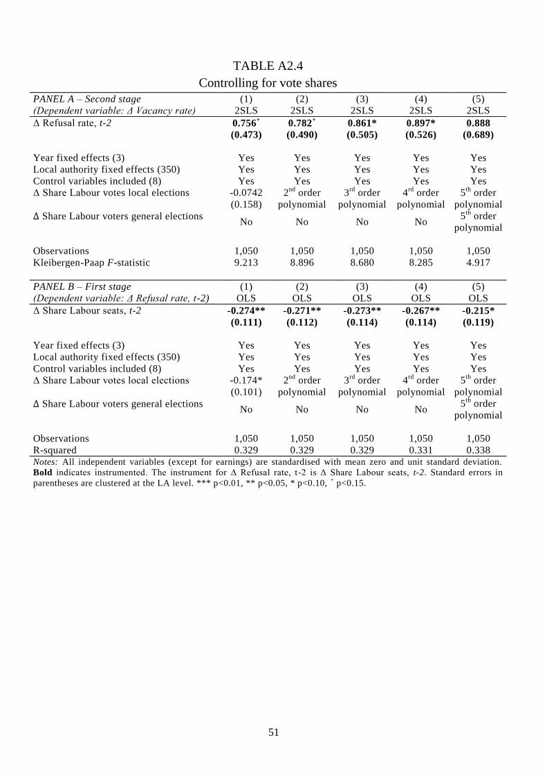
51

TABLE A2.4

Controlling for vote shares

PANEL A – Second stage (1) (2) (3) (4) (5)

(Dependent variable: Δ Vacancy rate) 2SLS 2SLS 2SLS 2SLS 2SLS

Δ Refusal rate, t-2 0.756+

0.782+

0.861* 0.897* 0.888

(0.473) (0.490) (0.505) (0.526) (0.689)

Year fixed effects (3) Yes Yes Yes Yes Yes

Local authority fixed effects (350) Yes Yes Yes Yes Yes

Control variables included (8) Yes Yes Yes Yes Yes

Δ Share Labour votes local elections -0.0742 2nd

order 3rd

order 4rd

order 5th

order

(0.158) polynomial polynomial polynomial polynomial

Δ Share Labour voters general elections No No No No

5th

order

polynomial

Observations 1,050 1,050 1,050 1,050 1,050

Kleibergen-Paap F-statistic 9.213 8.896 8.680 8.285 4.917

PANEL B – First stage (1) (2) (3) (4) (5)

(Dependent variable: Δ Refusal rate, t-2) OLS OLS OLS OLS OLS

Δ Share Labour seats, t-2 -0.274** -0.271** -0.273** -0.267** -0.215*

(0.111) (0.112) (0.114) (0.114) (0.119)

Year fixed effects (3) Yes Yes Yes Yes Yes

Local authority fixed effects (350) Yes Yes Yes Yes Yes

Control variables included (8) Yes Yes Yes Yes Yes

Δ Share Labour votes local elections -0.174* 2nd

order 3rd

order 4rd

order 5th

order

(0.101) polynomial polynomial polynomial polynomial

Δ Share Labour voters general elections No No No No

5th

order

polynomial

Observations 1,050 1,050 1,050 1,050 1,050

R-squared 0.329 0.329 0.329 0.331 0.338 Notes: All independent variables (except for earnings) are standardised with mean zero and unit standard deviation.

Bold indicates instrumented. The instrument for Δ Refusal rate, t -2 is Δ Share Labour seats, t-2. Standard errors in

parentheses are clustered at the LA level. *** p<0.01, ** p<0.05, * p<0.10, + p<0.15.

52

TABLE A2.5

Instrumenting for regulatory restrictiveness and earnings

PANEL A – Second stage

(Dependent variable: Δ Vacancy rate)

(1) (2) (3) (4)

2SLS 2SLS 2SLS 2SLS

Δ Refusal rate, t-2 0.814** 0.966** 0.816* 1.055**

(0.390) (0.387) (0.439) (0.498)

Δ Earnings (log) -0.257 4.469 6.370 4.149

(1.717) (5.170) (5.820) (5.114)

Year fixed effects (3) Yes Yes Yes Yes

Local authority fixed effects (350) No Yes Yes Yes

Control variables included (8) No No Yes Yes

Δ Share Labour voters local elections Ω( ∙ ) No No No Yes

Observations 1,050 1,050 1,050 1,050

Kleibergen-Paap F-statistic 9.660 5.467 3.714 3.610

PANEL B – First stage

(Dependent variable: Δ Refusal rate, t-2)

(1) (2) (3) (4)

OLS OLS OLS OLS

Δ Share Labour seats, t-2 -0.305*** -0.297*** -0.312*** -0.224*

(0.0702) (0.0957) (0.0981) (0.116)

Δ Labour demand shock 1971 (log) 2.121*** 6.953** 10.29*** 10.12***

(0.666) (2.843) (3.102) (3.159)

Year fixed effects (3) Yes Yes Yes Yes

Local authority fixed effects (350) No Yes Yes Yes

Control variables included (8) No No Yes Yes

Δ Share Labour voters local elections Ω( ∙ ) No No No Yes

Observations 1,050 1,050 1,050 1,050

Adj. R-squared 0.172 0.317 0.335 0.342

Angrist-Pischke F-statistic 14.12 14.17 19.00 12.24

PANEL C – First stage

(Dependent variable: Δ Earnings (log))

(1) (2) (3) (4)

OLS OLS OLS OLS

Δ Share Labour seats, t-2 0.00575 0.0119 0.00259 0.0140

(0.00864) (0.0117) (0.0106) (0.0124)

Δ Labour demand shock 1971 (log) 0.823*** 1.011*** 1.245*** 1.267***

(0.0809) (0.283) (0.326) (0.339)

Year fixed effects (3) Yes Yes Yes Yes

Local authority fixed effects (350) No Yes Yes Yes

Control variables included (8) No No Yes Yes

Δ Share Labour voters local elections Ω( ∙ ) No No No Yes

Observations 1,050 1,050 1,050 1,050

R-squared 0.406 0.557 0.616 0.622

Angrist-Pischke F-statistic 51.73 9.56 11.30 10.67 Notes: Bold indicates instrumented. The instruments for Δ Refusal rate and Δ Earnings (log) are Δ Share of Labour

seats and Δ Labour demand shock 1971 (log). Standard errors in parentheses are clustered at the LA level. ***

p<0.01, ** p<0.05, * p<0.10, + p<0.15.

53

TABLE A2.6

Additional sensitivity checks – second stage results

(1) (2) (3) (4) (5)

Exclude

Greater

London

Refusal

rate for all

projects

Fixed effects

approach –

no trends

Fixed effects

approach –

linear trends

Fixed effects

approach – non-

linear trends

2SLS 2SLS 2SLS 2SLS 2SLS

Δ Refusal rate, t-2 1.218**

(0.511)

Δ Refusal rate for all projects, t-2 1.124*

(0.673)

Refusal rate, t-2 0.757** 0.714** 1.822***

(0.346) (0.294) (0.690)

Control variables included (8) Yes Yes Yes Yes Yes

Δ Share Labour voters local elections Ω( ∙ ) Yes Yes Yes Yes Yes

Share Labour voters local elections Ω( ∙ ) Yes Yes Yes Yes Yes

Local authority fixed effects (350) Yes Yes Yes Yes Yes

Local authority linear trends (350) No No No Yes Yes

Local authority non-linear trends (350) No No No No Yes

Year fixed effects (3) Yes Yes Yes Yes Yes

Observations 954 1,050 1,400 1,400 1,400

Kleibergen-Paap F-statistic 9.608 2.962 17.52 16.63 5.081 Notes: All independent variables (except for earnings) are standardised with mean zero and unit standard deviation.

Bold indicates instrumented. The instrument for (Δ) Refusal rate is (Δ) Share of Labour seats in the LA. Ω( ∙ ) is

approximated by a fifth-order polynomial of share Labour voters. Standard errors in parentheses are clustered at the LA

level. *** p<0.01, ** p<0.05, * p<0.10, + p<0.15.

54

TABLE A2.7

Results using Census data (1981-2001) and DCLG data (2001-2011)

(Dependent variable: Δ Vacancy rate)

(1) (2) (3) (4) (5) (6) (7)

OLS OLS OLS 2SLS 2SLS 2SLS 2SLS

Δ Refusal rate, t-2 0.100*** 0.141*** 0.115** 0.961*** 1.040*** 0.917*** 0.780*

(0.0375) (0.0502) (0.0472) (0.350) (0.348) (0.308) (0.429)

Year fixed effects (3) Yes Yes Yes Yes Yes Yes Yes

Local authority fixed effects (350) No Yes Yes No Yes Yes Yes

Control variables included (8) No No Yes No No Yes Yes

Δ Share Labour voters local elections Ω( ∙ ) No No No No No No Yes

Observations 1,050 1,050 1,050 1,050 1,050 1,050 1,050

R-squared 0.294 0.468 0.522

Kleibergen-Paap F-statistic 18.56 17.61 19.09 8.212

Notes: All independent variables (except for earnings) are standardised with mean zero and unit standard deviation. Bold indicates instrumented. In Models (4)-(7), the

instrument for Δ Refusal rate is Δ Share of Labour seats in the LA. Ω( ∙ ) is approximated by a fifth-order polynomial of share Labour voters in local elections. Standard

errors in parentheses are clustered at the LA level. *** p<0.01, ** p<0.05, * p<0.10, + p<0.15.

55

TABLE A2.8

Results using Census data (1981-2001, excluding 2011)

PANEL A – Second stage (1) (2) (3) (4) (5) (6) (7)

(Dependent variable: Δ Vacancy rate) OLS OLS OLS 2SLS 2SLS 2SLS 2SLS

Δ Refusal rate, t-2 0.123** 0.191** 0.114 1.121 2.483* 2.321* 2.844

(0.0490) (0.0896) (0.0702) (0.697) (1.278) (1.401) (2.467)

Year fixed effects (2) Yes Yes Yes Yes Yes Yes Yes

Local authority fixed effects (350) No Yes Yes No Yes Yes Yes

Control variables included (8) No No Yes No No Yes Yes

Δ Share Labour voters local elections Ω( ∙ ) No No No No No No Yes

Observations 700 700 700 700 700 700 700

R-squared 0.412 0.620 0.736

Kleibergen-Paap F-statistic 7.528 4.365 2.939 1.355

PANEL B – First stage (4) (5) (6) (7)

(Dependent variable: Δ Refusal rate, t-2) OLS OLS OLS OLS

Δ Share Labour seats, t-2 -0.243*** -0.255 -0.219 -0.163

(0.0886) (0.173) (0.182) (0.200)

Year fixed effects (2) Yes Yes Yes Yes

Local authority fixed effects (350) No Yes Yes Yes

Control variables included (8) No No Yes Yes

Δ Share Labour voters local elections Ω( ∙ ) No No No Yes

Observations 700 700 700 700

R-squared 0.070 0.358 0.375 0.385 Notes: All independent variables (except for earnings) are standardised with mean zero and unit standard deviation. Bold indicates instrumented. In Models (4)-(7), the

instrument for Δ Refusal rate is Δ Share of Labour seats in the LA. Ω( ∙ ) is approximated by a fifth-order polynomial of share Labour voters in local elections. Standard

errors in parentheses are clustered at the LA level. *** p<0.01, ** p<0.05, * p<0.10, + p<0.15.

W1

WEB APPENDIX: Theoretical Model

W1. Matching and sales time

We analyse a setting with search frictions where households may move, but not freely,

between housing markets. We extend the seminal house price bargaining model by Wheaton

(1990), which can be interpreted as a model with two symmetric housing markets. We follow

Koster and Van Ommeren (2017) by relaxing the symmetry assumption. This is needed to

analyse the effects of more stringent land use regulations in one of the two housing markets.

We first outline the model and discuss the relationship between search effort, matching rates,

house prices and regulatory restrictiveness. Using numerical simulations, we then illustrate

that regulatory restrictions may both increase or decrease the (relative) vacancy rate, while

they will lead to relatively higher prices and lower matching rates.

Assume a country with a given number of home-owning households equal to2�̅�. The country

consists of two local housing markets each with 𝑆𝑖 identical housing units, where 𝑖 = 1,2.

Households own at least one house but may own two houses. All houses, including vacant

ones, are owned by a household implying that (𝑆̅ − �̅�) �̅�⁄ < 0.5. Households prefer to live in

one of the two housing markets. Let 𝐻𝑖 denote the number of households who prefer to live in

housing market 𝑖, where 𝑖 = 1, 2. Households who live in their preferred housing market are

matched, otherwise they are mismatched. Mismatched households search for housing in the

other housing market. Dual-ownership households have a house in both housing markets, are

therefore matched, but own a vacant house in the other housing market.

Preferences for a housing market change over time at an exogenous rate 𝛽. For example, the

location of the job may be exogenously changed from one housing market to the other due to

a firm relocation (Mulalic et al., 2014). The change over time in 𝐻𝑖 denoted by �̇�𝑖 =

𝛽(𝐻𝑗 − 𝐻𝑖) for 𝑖 ≠ 𝑗. In what follows, 𝑗 will always denote the other housing market. The

total endogenously determined number of households that have a preference to reside in 𝑖 is

given by 𝐻𝑖 = 𝐻𝑖𝑀 + 𝐻𝑖

𝐷 + 𝐻𝑖𝑆, where 𝐻𝑖

𝑀 is the number of matched households with one

house, 𝐻𝑖𝐷 is the number of households possessing two houses, and 𝐻𝑖

𝑆 denotes the number of

mismatched households.

By construction, the vacancy rate in a housing market 𝑣𝑖 equals housing supply 𝑆𝑖 minus the

number of households living there divided by the number of housing units in 𝑖. Because

mismatched households 𝑗 live in housing market 𝑖, the following holds:

(1) 𝑣𝑖 =𝐻𝑗

𝐷

𝑆𝑖=

𝑆𝑖 − 𝐻𝑖𝐷 − 𝐻𝑖

𝑀 − 𝐻𝑗𝑆

𝑆𝑖.

Each vacant house is owned by a household that lives in the other housing market, so

𝐻𝑖𝐷 = 𝑣𝑗𝑆𝑗 where 𝑖 ≠ 𝑗. Hence, the number of vacant housing units in housing market j is

equal to the number of dual-ownership households living in housing market i. Mismatched

households search for houses in the other housing market and given a contact with a vacancy

in that housing market, they find a (suitable) house with probability one. Matching of

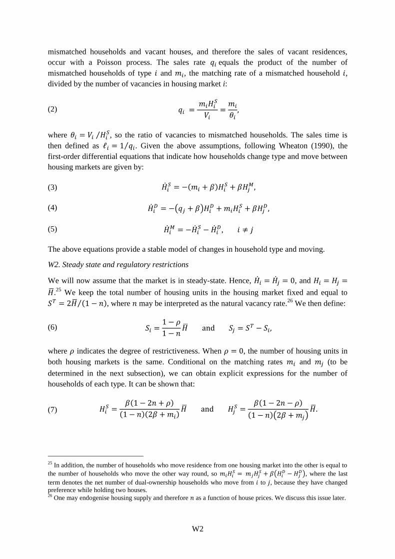
W2

mismatched households and vacant houses, and therefore the sales of vacant residences,

occur with a Poisson process. The sales rate 𝑞𝑖 equals the product of the number of

mismatched households of type 𝑖 and 𝑚𝑖, the matching rate of a mismatched household 𝑖,

divided by the number of vacancies in housing market i:

(2) 𝑞𝑖 = 𝑚𝑖𝐻𝑖

𝑆

𝑉𝑖=

𝑚𝑖

𝜃𝑖,

where 𝜃𝑖 = 𝑉𝑖 𝐻𝑖𝑆⁄ , so the ratio of vacancies to mismatched households. The sales time is

then defined as ℓ𝑖 = 1 𝑞𝑖⁄ . Given the above assumptions, following Wheaton (1990), the

first-order differential equations that indicate how households change type and move between

housing markets are given by:

(3) �̇�𝑖𝑆 = −(𝑚𝑖 + 𝛽)𝐻𝑖

𝑆 + 𝛽𝐻𝑗𝑀,

(4) �̇�𝑖𝐷 = −(𝑞𝑗 + 𝛽)𝐻𝑖

𝐷 + 𝑚𝑖𝐻𝑖𝑆 + 𝛽𝐻𝑗

𝐷 ,

(5) �̇�𝑖𝑀 = −�̇�𝑖

𝑆 − �̇�𝑖𝐷, 𝑖 ≠ 𝑗

The above equations provide a stable model of changes in household type and moving.

W2. Steady state and regulatory restrictions

We will now assume that the market is in steady-state. Hence, �̇�𝑖 = �̇�𝑗 = 0, and 𝐻𝑖 = 𝐻𝑗 =

�̅�.25

We keep the total number of housing units in the housing market fixed and equal to

𝑆𝑇 = 2�̅� (1 − 𝑛)⁄ , where 𝑛 may be interpreted as the natural vacancy rate.26

We then define:

(6) 𝑆𝑖 =1 − 𝜌

1 − 𝑛�̅� and 𝑆𝑗 = 𝑆𝑇 − 𝑆𝑖,

where 𝜌 indicates the degree of restrictiveness. When 𝜌 = 0, the number of housing units in

both housing markets is the same. Conditional on the matching rates 𝑚𝑖 and 𝑚𝑗 (to be

determined in the next subsection), we can obtain explicit expressions for the number of

households of each type. It can be shown that:

(7) 𝐻𝑖𝑆 =

𝛽(1 − 2𝑛 + 𝜌)

(1 − 𝑛)(2𝛽 + 𝑚𝑖)�̅� and 𝐻𝑗

𝑆 =𝛽(1 − 2𝑛 − 𝜌)

(1 − 𝑛)(2𝛽 + 𝑚𝑗)�̅�.

25

In addition, the number of households who move residence from one housing market into the other is equal to

the number of households who move the other way round, so 𝑚𝑖𝐻𝑖𝑆 = 𝑚𝑗𝐻𝑗

𝑆 + 𝛽(𝐻𝑖𝐷 − 𝐻𝑗

𝐷), where the last

term denotes the net number of dual-ownership households who move from 𝑖 to 𝑗, because they have changed

preference while holding two houses. 26

One may endogenise housing supply and therefore 𝑛 as a function of house prices. We discuss this issue later.

W3

Given the latter equality, we obtain the intuitive result that the number of mismatched

households in 𝑖 depends negatively on the matching rate 𝑚𝑖 (but does not depend on the

matching rate of the other housing market 𝑚𝑗).27

It is also observed that the matching rate in 𝑖

depends positively on regulatory restrictiveness, while the number of mismatched households

in 𝑗 decreases when 𝜌 is higher. We may also interpret this as an indirect way of commuting

distance. If 𝛽 signals the workplace, a higher 𝐻𝑖𝑆 will imply a longer workplace commute

distance from 𝑖 because mismatched households of type 𝑖 still live in 𝑗.

Similarly, the number of matched households in i can be written as:

(8) 𝐻𝑖𝑀 =

(1 − 2𝑛 − 𝜌)(𝛽 + 𝑚𝑗)

(1 − 𝑛)(2𝛽 + 𝑚𝑗)�̅� and 𝐻𝑗

𝑀 =(1 − 2𝑛 + 𝜌)(𝛽 + 𝑚𝑖)

(1 − 𝑛)(2𝛽 + 𝑚𝑖)�̅�

which is an increasing function of the matching rate in the other housing market, but does not

depend on the own matching rate. From (8), it can be immediately seen that restrictions

reduce the number of matched households in 𝑖.

The vacancy rate 𝑣𝑖 is equal to the number of dual owners in housing market 𝑗 divided by the

housing supply in 𝑖. Using (1), (6), (7) and (8):

(9) 𝑣𝑖 =𝛽 ((𝜌 − 1)𝑚𝑗 − 4𝑛𝛽) + 𝑚𝑖 ((1 − 4𝑛 + 𝜌)𝛽 − (𝑛 − 𝜌)𝑚𝑗)

(𝜌 − 1)(2𝛽 + 𝑚𝑖)(2𝛽 + 𝑚𝑗),

It is more informative to evaluate the derivative of the vacancy rate with respect to

restrictions:

PROPOSITION 1 [Vacancy rate effect of restrictions]: Restrictions may either positively or

negatively affect vacancy rates, d𝑣𝑖 d𝜌⁄ ⋚ 0.

Proof. The derivative of (9) is given by:

(10) 𝜕𝑣𝑖

𝜕𝜌=

(𝑛 − 1)𝑚𝑖

2𝛽 + 𝑚𝑖+

2𝑛𝛽2𝛽 + 𝑚𝑗

(𝜌 − 1)2,

The denominator is always positive. In the presence of regulations, the vacancy rate will

increase when the natural vacancy rate is high relative to the matching rates 𝑚𝑗. Also when

𝑚𝑖 → 0 (but 𝑚𝑗 is not close to zero), (10) becomes positive, so in inefficient markets with

low matching rates, restrictions may lead to increases in vacancy rates.

27

In line with intuition, when 𝑚𝑖 approaches infinity, so search frictions in i are absent, the number of

mismatched households of type 𝑖 (who live in j) approaches zero.

W4

W3. Matching and house prices

In the previous subsection, matching rates were given. We will now assume that matching

rates are endogenously determined. Mismatched households choose the level of search effort

𝑒𝑖 to find a new house. We assume a constant return to scale Cobb-Douglas matching

function, following the theoretical and empirical literature on labour market matching:

(11) 𝑚𝑖 = 𝜇𝑒𝑖𝜓

𝜃𝑖1−𝜓

,

where 𝜇 is a constant. Note again that 𝜃𝑖 = 𝑉𝑖 𝐻𝑖𝑆⁄ .

The level of search effort is based on the households’ present discounted value of being in a

certain state, which depends, among others, on house prices. In steady state, the value of a

certain state can be written as the utility flow of being in that state plus the value of changing

state:

(12) 𝑟𝑢𝑖𝑀 = 𝐴𝑖 + 𝛽(𝑢𝑗

𝑆 − 𝑢𝑖𝑀),

(13) 𝑟𝑢𝑖𝐷 = 𝐴𝑖 + 𝑞𝑗(𝑢𝑖

𝑀 − 𝑢𝑖𝐷 + 𝑝𝑗) + 𝛽(𝑢𝑗

𝐷 − 𝑢𝑖𝐷) ,

(14) 𝑟𝑢𝑖𝑆 = −𝑐𝑖 + 𝛽(𝑢𝑗

𝑀 − 𝑢𝑖𝑆) + 𝑚𝑖(𝑢𝑖

𝐷 − 𝑢𝑖𝑆 − 𝑝𝑖), 𝑖 ≠ 𝑗

where 𝑢𝑖𝑀, 𝑢𝑖

𝐷, 𝑢𝑖𝑆 are the present values of each state (matched, dual ownership,

mismatched), 𝐴𝑖 refers to the utility flow of the housing market-specific amenity, 𝑟 is the

discount rate, 𝑐𝑖 is the cost of search and 𝑝𝑖 is the house price. Matched and dual-owners

households of type 𝑖 enjoy the housing market-specific amenity 𝐴𝑖 , see (12) and (13),

whereas mismatched households of type 𝑖 (who live in 𝑗) do not enjoy 𝐴𝑗.28

Households are

assumed to choose the level of search effort 𝑒𝑖 to maximise 𝑢𝑖𝑆.

In equation (14), it is assumed that mismatched households incur search costs 𝑐𝑖 as a function

of search effort. We will assume that 𝑐𝑖 = 𝑒𝑖2 2⁄ , so 𝑐𝑖 is an increasing and convex function of

search effort.29

Here, we only consider symmetric equilibria where all households choose the same search

effort level. The individual matching rate of a mismatched household of type i is the product

of individual search effort and the average number of matches in the point where �̃�𝑖 = 𝑒𝑖,

where �̃�𝑖 is the individual level of search effort.30

Then:

28

If one assumes that mismatched households receive a positive share of 𝐴𝑗, results will not change. 29

We may also assume that dual ownership households incur search costs. However, because we will allow for

bargaining on the price later on, this will not change the outcomes of the model, while it unnecessarily

complicates matters. 30

This means that the second-order derivative of the matching rate with respect to individual search effort is

equal to zero.

W5

(15) 𝜕𝑚𝑖

𝜕�̃�𝑖=

𝑚𝑖

𝑒𝑖,

The marginal cost from an additional unit of search effort is equal to the marginal

benefit of that unit. Given equation (14), optimal choice of search effort implies:

(16) 𝜕𝑐𝑖

𝜕�̃�𝑖=

𝜕𝑚𝑖

𝜕�̃�𝑖(𝑢𝑖

𝐷 − 𝑢𝑖𝑆 − 𝑝𝑖) ,

where 𝑢𝑖𝐷 − 𝑢𝑖

𝑆 − 𝑝𝑖 indicates the benefit of a match for mismatched households.

In a general equilibrium setting, prices are endogenous. We assume that buyers and sellers

bargain about prices using Nash-bargaining, where buyers get a fixed share 𝜎 of the total

benefits of the match. So, 𝑢𝑖𝐷 − 𝑢𝑖

𝑆 − 𝑝𝑖 = 𝜎(𝑢𝑖𝐷 − 𝑢𝑖

𝑆 + 𝑢𝑗𝑀 − 𝑢𝑗

𝐷) and hence 𝑝𝑖 =

𝜎(𝑢𝑗𝐷 − 𝑢𝑗

𝑀) + (1 − 𝜎)(𝑢𝑖𝐷 − 𝑢𝑖

𝑆).

W4. Numerical simulations

In this subsection we show that under reasonable parameter values, vacancy rates may be

positively associated with regulatory restrictiveness. We assume that 2�̅� = 1900, 𝛽 = 𝑛 =

0.15, 𝜌 = 0.1. We furthermore assume that sellers and buyers have equal bargaining power

(𝜎 = 0.5) and the interest rate is 2.5 percent (𝑟 = 0.025). The amenity 𝐴 level is set to 10 in

both housing markets. We analyse the outcomes when the market is in steady state. The

model is solved using an iterative two-step procedure.31

In Figure W1 we plot the matching

rates in 𝑖 and 𝑗 as a function of the matching constant 𝜇. Given the first order condition of

(16), when 𝜇 increases search effort will be higher and matching rates are higher because it is

more costly to leave a property vacant essentially. It is shown that the matching rate in 𝑖 is

always lower than in 𝑗 given restrictions in 𝑖 (the refusal rate is set to 0.1). Figure W2 shows

that vacancy rates in 𝑖 are only higher than in 𝑗 when the matching constant is smaller. That

is, when the opportunity costs of leaving a property empty are not too high. Figure W3

confirms the empirical stylised fact that prices in restrictive local housing markets are above

the house prices of less restrictive housing markets. We note that one may also endogenise

housing supply as a function of prices. This would mean that, conditional on supply

restrictions, supply would increase in the more restrictive housing market 𝑖. This means that

the vacancy rate in 𝑖 would increase even more, amplifying the positive effect of restrictions

on vacancy rates.

31

First, conditional on an initial (arbitrary) choice of values for number of household variables 𝐻𝑖𝑆, 𝐻𝑗

𝑆, 𝐻𝑖𝑀 and

𝐻𝑗𝑀, we solve for house prices, optimal search effort in both areas. Given optimal search effort, we determine

𝑚𝑖, 𝑚𝑗, 𝑞𝑖 and 𝑞𝑗. Given these values, we calculate the number of households in each state using equations (3)

to (5). We continue this process until the model converges.

W6

FIGURE W1

Matching rates and restrictions

FIGURE W2

Vacancy rates and restrictions

0.00

0.50

1.00

1.50

2.00

2.50

3.00

3.50

4.00

4.50

5.00

0.00 0.25 0.50 0.75

Ma

tch

ing

ra

te

Matching constant, μ

i j

0.130

0.135

0.140

0.145

0.150

0.155

0.160

0.165

0.170

0.00 0.25 0.50 0.75

Vaca

ncy

rate

Matching constant, μ

i j

W7

FIGURE W3

House prices and restrictions

Web appendix references

Koster, H.R.A. and Van Ommeren, J.N. (2017) On Housing Search Frictions: Hedonic Price

Models, Optimal Search and Welfare. Mimeo, Vrije Universiteit Amsterdam.

Mulalic, I., Van Ommeren, J. N., and Pilegaard, N. (2014) Wages and Commuting: Quasi-

natural Experiments’ Evidence from Firms that Relocate. Economic Journal 124: 1086-

1105.

Wheaton, W.C. (1990). Vacancy, Search, and Prices in a Housing Market Matching Model.

Journal of Political Economy 98(6): 1270-1292.

0

50

100

150

200

250

300

350

400

0.00 0.25 0.50 0.75

Ho

use

pri

ce

Matching constant, μ

i j