Enabling Advanced Operational Analysis Through Multi-Subsystem DataIntegration on Trinity

J. Brandt∗, D. DeBonis∗, A. Gentile∗, J. Lujan†, C. Martin†,D. Martinez∗, S. Olivier∗, K. Pedretti∗, N. Taerat‡, and R. Velarde†

∗Sandia National LaboratoriesAlbuquerque, NM

Email:(brandt|ddeboni|gentile|davmart|slolivi|ktpedre)@sandia.gov†Los Alamos National Laboratory

Los Alamos, NMEmail:(jewel|c martin|ronv)@lanl.gov

‡Open Grid ComputingAustin, TX

Email:narate@ogc.us

Operations management of the New Mexico Alliancefor Computing at Extreme Scale (ACES) (a collabora-tion between Los Alamos National Laboratory and SandiaNational Laboratories) Trinity platform will rely on datafrom a variety of sources including System EnvironmentData Collections (SEDC); node level information, such ashigh speed network (HSN) performance counters and highfidelity energy measurements; scheduler/resource manager;and plant environmental facilities. The water-cooled CrayXC platform requires a cohesive way to manage both thefacility infrastructure and the platform due to several criticaldependencies. We present preliminary results from analysisof integrated data on the Trinity Application ReadinessTestbed (ART) systems as they pertain to enabling advancedoperational analysis through the understanding of opera-tional behaviors, relationships, and outliers.

Keywords-High Performance Computing; Monitoring

I. INTRODUCTION

At the same time HPC platform scale is increasing,systems are also becoming more heterogeneous in computa-tional, storage, and networking technologies. As the volumeand complexity of information continues to increase it willbecome impossible to efficiently manage platforms withouttools that perform run-time analysis continuously on allavailable data and take appropriate action with respect toproblem resolution and power management. An exampleof the complex interplay that advanced analysis tools canbe used to aid in understanding is variation in applicationperformance due to network congestion, contention for

Sandia National Laboratories is a multi-program laboratory managed andoperated by Sandia Corporation, a wholly owned subsidiary of LockheedMartin Corporation, for the U.S. Department of Energy’s National NuclearSecurity Administration under contract DE-AC04-94AL85000.

LA-UR-15-23103

shared parallel file system bandwidth, contention for burstbuffer bandwidth, thermally related CPU throttling, workingbut faulty hardware/firmware, and more. Any or all of theabove conditions can cause wide variation in applicationperformance but without simultaneous access to monitoredfacilities data, system data, system logs, console logs, eventlogs, etc., correct diagnosis and problem resolution willbecome impossible.

Additionally, large scale HPC platforms are now pushingthe limits of data center power and cooling infrastructure.Modern large scale platforms with power draw requirementsin the 20MW range can stress data center and site powerinfrastructure (e.g., power demands that change abruptlycan cause power disruption in the data center and possiblyincluding the local power grid). Thus the ability to prior-itize and manage platform power allocations is becomingessential and active management of a platform’s average andpeak power draw through processor frequency management(another parameter that affects performance) has become ahigh priority for both HPC data centers and vendors and iscurrently a hot research topic.

Relatedly, the increase in power density of HPC compo-nents has necessitated the use of water based solutions forheat transport rather than traditional air cooling solutions.This in turn requires feedback mechanisms to maintainproper water temperature, pressure, and flow rates as wellas active fan control in the case of hybrid solutions.

Traditionally our HPC platforms, both current and past,have had stove-piped monitoring operations where informa-tion rarely crossed the boundaries of responsibility betweenfacilities and platform operation. Data centers monitoredpower and cooling at a plant level and HPC system adminis-trators monitored platform level variables such as system andevent logs. Only when the platform environment was deemedto be the cause of problems would there be communications

between the two groups about their respective data andhow it was pertinent. However, upcoming pre- and exascaleplatforms will have the potential to incur large monetary costand even cause site wide disruption to power if operatedblindly.

Thus, in order to maximize the value of modern large scaleplatforms a management approach that tightly integrates allinformation both internal and external to the platforms isrequired. The ability to control data center infrastructure dy-namically based on platform, job, power, and environmentalinformation will become a necessity as we move towardsexascale computing.

In this paper we present how we are planning on per-forming such information integration to efficiently manageTrinity, the upcoming ACES Cray XC40 platform. We showhow we are utilizing our Application Readiness Testbed(ART) systems to prototype and validate our planned con-figuration with a particular eye to power, thermal, and datacenter facilities data. We first present our ART system andmonitoring configurations in Section II. Next we describethe various sources of information along with how they arebeing collected/aggregated in Section III. In order to producedata under normal operating conditions we put togethera workload to run on the system which is described inSection IV. Select data along with analysis of its pertinenceis presented in Section V. Finally we present conclusionsand future work plans in Section VI.

II. SYSTEM CONFIGURATION AND MONITORING SETUP

Trinitite and Mutrino are ART systems obtained to preparefor Trinity with respect to the applications that will berun. Additionally, they provide platforms for validation offacilities–platform interaction and comparison. Most of thetesting and measurements presented in this paper wereperformed on Trinitite, a single cabinet Cray XC40 at LosAlamos National Laboratory (LANL), where Trinity willalso be sited. We also present some comparisons betweenbehaviors of Trinitite and an identical system, Mutrino, sitedat Sandia National Laboratories (SNL), in Section V. TheART systems were delivered in February 2015.

In this section we first describe the basic configuration ofour ART systems. We provide insight, at a high level, aboutour integrated monitoring configuration, what informationwe are collecting, and our information aggregation andprocessing approaches. Finally we discuss the mechanismsused for transport of data from the various sources to acommon system for processing. Note that the monitoringinfrastructure on the full Trinity system will be distributed.

A. System Configuration

Our ART systems are single cabinet water cooled CrayXC40’s populated with 100 compute nodes and 18 servicenodes (the rack is not fully populated with server blades).The service nodes have the following functionalities: 1

Figure 1. High Level Monitoring Diagram showing ART related informa-tion sources and their data feeds to a Monitor host

logins, 6 burst buffer, 2 MOMs, 2 DVS, 3 LNet routers,2 sdb (1 failover) and 2 boot (1 failover). Additionallylinux white boxes are provided for: external login, SystemManagement Workstation (SMW), and Power ManagementNode (PMN). The PMN is currently being utilized as aMonitor host. All compute nodes and service nodes utilizethe Cray Aries interconnect in a dragonfly configuration [1].Each compute node is configured with dual 16 core IntelHaswell processors running at 2.3GHz and 64GB of mem-ory. The external connections consist of FDR Infiniband toLustre storage (Sonexion), and 40/10 Gigabit Ethernet toSMW, sdb, external login, and PMN. The public networkconnections are 10 Gigabit Ethernet.

B. Monitoring Setup

Figure 1 depicts the current HPC platform componentsin the colored band with all monitored data, including thatfrom the data center infrastructure, being sent/forwarded toa Monitor host deployed specifically for data aggregation,analysis, and both short and long term storage of the data.This scenario will change with the full Trinity system in thatthere will be several Monitor hosts for both scalability andredundancy with the 10K nodes depicted in the figure beingan upper bound on what a Monitor host would be expected toprocess. As shown all monitored data will be aggregated toa set of Monitor hosts which will serve as data aggregation,storage, and both run-time analysis and post processing.This is the approach we have taken with data gathering forthis paper where the Monitor box here is represented bythe PMN block in Figure 2. The exceptions were that ourdata center infrastructure monitoring was performed out-of-band as described in Section III-E and we supplementedthe SEDC and power data as described in Sections III-Fand III-C.

Node level data collection is performed by LightweightDistributed Metric Service (LDMS) samplers (Section III-D)running on every host (including login) as shown in Figure 2.Aggregators for this information run on service nodes (alogin node in this case) and collect data at regular timeintervals using Remote Direct Memory Access (RDMA)to minimize compute node CPU overhead. Aggregators

Figure 2. Application Readiness Testbed (ART) Connectivity Diagramshowing how the major components of the platforms are interconnected

running on the Monitor hosts collect this data from theaggregators running on the service nodes and store the data.The aggregators running on the Monitor hosts are also capa-ble of doing analysis on the data as it is streaming throughand will ultimately be able to provide notification of outlierbehavior. Note that the out-of-band Hardware SupervisorySystem (HSS) network exists but is not shown. All log filesand SEDC data are forwarded to the Monitor from the SMW.On the full Trinity platform each Monitor will be receivinga fraction of the SEDC data with appropriate redundancyfor failure mitigation.

III. DATA SOURCES

In this work we utilize data from a variety of sourcesincluding System Environment Data Collections (SEDC),node level information, scheduler/resource manager, anddata center environmental sensors. The SEDC data providesinformation about voltages, currents, and temperatures ofa variety of components at the cabinet, blade, and nodelevel. This data also includes dew point, humidity andair velocity information. While the system utilizes manyof these measurements to identify out of spec, and henceunhealthy, components it relies on fixed thresholds beingcrossed to trigger knowledge of an unhealthy situation.The node level information provides high fidelity energymeasurements, OS level counters, and high speed networkperformance counters. Scheduler/resource manager informa-tion provides time windows and components associated withuser applications. Data center environmental data providesfine grained power draw, information about noise on thepower feeds, and water temperatures and flow rates.

A. Logs

Logging when errors or meaningful transitions occuris used by many subsystems as a means of providingsystem administrators and troubleshooters with diagnosticinformation. On the Cray XC system many sources oflog information exist: syslog, console, power management,smw, event, Application Level Placement Scheduler (ALPS),etc. All of these logs are forwarded from various components

to the SMW and placed in appropriate directories. In orderto make them available for analysis in conjunction with therest of the data we are collecting, we forward all log files toour Monitor host using rsyslog. This data path is depictedin Figure 1.

B. System Environmental Data Collections (SEDC)

Cray’s System Environment Data Collections (SEDC) [2]provides a rich source of environmental data for many lowlevel system components such as CPUs, memory, powersupplies, nodes, blades, and more. The beauty of this in-formation is that it is completely out-of-band with respectto node level computation and network communication.While the typical (default) configuration is to push theSEDC data to an aggregation point (the SMW) over theHardware Supervisory System (HSS) network at 60 secondintervals, we configured it to be pushed at 1 second intervalsand configured rsyslog on the SMW to forward it to ourMonitor host. One of the problems we see with the currentconfiguration is that independent of platform size, all SEDCdata is configured to go directly to the SMW. This presentsa bottleneck to storage and parallel processing of this data.Ultimately we would like the ability to incorporate otherdevices, such as our Monitor hosts, into the HSS networkand have the SEDC data distributed across them.

Some of the data that should have been available viathe SEDC data stream was missing i.e., all cooling waterrelated data, such as temperatures, pressures, and flow rates,was not present. Additionally it should be noted that whileCPU Package energies units are defined as Joules in theSEDC scanID file, the actual data appears to be in units ofmilli-Joules (mJ). We did not use this data for comparisonpurposes in this paper as we could not validate that it wasactually calibrated in mJ. Cray [3] states these bugs are fixedin CLE7.2 UP03 and CLE7.2 UP04 respectively.

C. Power API

We use the Power API prototype, which is a referenceimplementation of the Power API specification version1.0[4] released to the HPC community in September of2014, to collect node level data at 10Hz. The Power APIspecification describes a comprehensive system softwareAPI for interfacing with power measurement and controlhardware. The specification defines the system model, theoryof operations, and features exposed, covering the facilitylevel down to low level software / hardware interfaces. Theprototype supports most core features of the Power APIspecification. The prototype is a layered architecture thatconforms to the specification and provides rich descriptivesystem configuration semantics, supports runtime plugins fora variety of devices and resources, and enables distributedcommunication for remote invocations of capabilities (seeFigure 3).

Power APICORE FEATURES

Device PluginXTPM

System DescriptionXML Config

DaemonXML RPC

SQL

Database

XML

Document

hwloc PowerInsight RAPL XTPM

WattsUp PowerGadget

Figure 3. Framework of the Power API Prototype

For our study, we describe our system using a nodelevel XML configuration file and utilize a plugin specificallycreated for the Cray platform which gains us access to thepower management features of the system. The combinationof the configuration file and XTPM plugin allow us to ab-stract the mechanisms of measurement and control from thespecifics of the platform by mapping Power API attributes tothe underlying plugin sysfs exposed parameters. We gathereddata at a sample rate of 10Hz for each node of the systemusing this facility. In this case data was saved to a sharedfile system for post processing. In the future we will useLDMS (Section III-D) to transport this data directly to theMonitor for run-time processing.

Note that while Cray provides power monitoring capabil-ities and a power management database (PMDB) for storingand querying power utilization data, these are inadequatefor our purposes. The power monitoring capability collectsat lower frequencies than we are interested in investigating,and even when higher frequency data can be obtained, itis limited in its ability to handle large numbers of nodesand long time periods [5]. Additionally, the power databaseis located on the SMW, which has inherent limitations inaccess and size, while we seek to enable continuous, near-indefinite runtime and historical analysis integrated withother data sources. For these reasons, we do not includethe power management database as source of data in thiswork. For convenience, however, we do use RUR output forsome general, relative, overall application energy utilization.

D. Lightweight Distributed Metric Service (LDMS)

We use LDMS [6] for node level data collection andtransport via the High Speed Network (HSN). This informa-tion, collected at 1Hz, includes HSN performance counters,Lustre client activity, application memory utilization, andother counters exposed by the OS. As of this writing LDMScollects node level energy data from the sysfs interface at1Hz. The LDMS energy sampler plugin will be upgraded tocollect 10Hz power/energy data via the Power API prototype(see Section III-C) thus making this full fidelity (10Hz)data available at 1Hz across the whole system. Use of thePower API will enable platform independent development of

LDMS power data collection plugins that can take advantageof new power related features as they are developed withoutnecessitating rewriting of the LDMS plugins.

The High Speed Network (HSN) performance counterdata is exposed via Cray’s gpcdr kernel module through thesysfs interface. While this module has been utilized for overa year on NCSA’s Blue Waters platform (Cray XE/XK),this is our first use of it on a Cray XC. This exposed asmall problem with the default gpcdr configuration whichexposed 160 counters via a single sysfs file. While thisconfiguration is ok when the counter values are small, itcauses the aggregate size to exceed the 4KB limit imposedon sysfs entries as the values become large. The authorat Cray quickly diagnosed the root cause of our apparentcounter corruption and provided us with a simple fix whichwas to divide the initial set into 4 smaller sets based oninformation type (traffic, stalls, receive link status, and sendlink status) [7]. This required only a slight modificationof the gpcdr configuration file and a reload of the kernelmodule.

We additionally collected the following non-HSN data viaLDMS:

• Lustre file system counters• CPU load averages• Current free memory• LNet traffic counters• ipogif counters• power and energy metrics via sysfs

E. Facilities

The facilities infrastructure that provides cooling to Trini-tite is composed of two main loops (Figure 4): the primaryand secondary cooling loops. These are separated by heatexchangers. The primary loop consists of four cooling towersand three pumps. The secondary loop consists of the threeheat exchangers and three pumps on variable frequencydrives (VFD).

The facility water supply temperature is 45oF at the inletto the heat exchangers. The secondary loop water supplytemperature to the machine and preconditioner is 75oF .

The building automation system that controls and mon-itors the facility cooling equipment is manufactured byTrane [8]. The Trinitite system and associated facility infras-tructure installation was substantially completed in February2015 and testing began in March 2015. Not all of thebuilding automation systems were operational for this testingtime frame.

The facilities data collected for this work was limited topower. Facilities power data was collected at five secondintervals from the compute rack feeder breaker using a Flukemeter 1730 Energy Logger. The Fluke meter was set tosample at 5KHz. It calculates an average over a five secondinterval as well as capturing the minimum and maximumvalues over that interval.

Figure 4. The Underfloor Pipe Diagram for the Data Center that housesTrinitite.

F. Envdata Script

Because the SEDC data stream currently does not containthe majority of the cooling water related data (see Sec-tion III-B) we have augmented our data collection usingthe envdata [9] script. From the SMW this script collectswater-related data directly from the cabinet. We called thescript at 10 second intervals and stored the output to disk forpost processing. Note that this is a stop-gap solution whichwill be discontinued once this data is included in the SEDCstream.

IV. WORKLOAD DESCRIPTION

For this work, we developed an application work packageto exercise the machine under a variety of conditions.Multiple iterations of single and multiple node runs of acombustion code, HPL, and HPCG were run as a group. Thisgroup was first run normally and then in turbo mode. Theserepeated cases we refer to as a Series. This Series was thenrun 3 times, once under each of the following conditions: nopower capping (415 Watts), 50% node level power capping(322 Watts), and 0% node level power capping (230 Watts).

HPL is the MPI implementation of the high perfor-mance Linpack benchmark [10]. A highly regular denseLU factorization, HPL is computationally intensive. HighPerformance Conjugate Gradient (HPCG) [11] is a verydifferent benchmark, by design. HPCG comprises opera-tions such as sparse matrix-vector products that stress thememory subsystem and network communications, and itsperformance may be uninhibited by modest reductions inCPU resources or frequency. HPL and HPCG represent ex-tremes in the spectrum of applications, from compute-boundto memory-bound, with orders-of-magnitude differences inFlops. In June 2014, Tianhe-2 reported the top numbers inboth benchmarks, with 33.9 Pflops on HPL but only 0.58Pflops on HPCG [12]. In addition to these benchmarks, wealso included in our system evaluation an application codefor direct numerical simulations of turbulent combustion. Ituses an explicit Runga-Kutta method with mostly nearestneighbor communications.

V. ANALYSIS AND RESULTS

In this work we combine information from log andnumeric data sources from both facilities and our ARTplatforms to expose issues facing all large scale HPC hostsites as we move to pre- and exascale platforms. In thissection we first present the analysis methodologies used inthis work. We then present both visual and analytic resultsof interest derived from data taken over a two day periodwhile running the workload as described in Section IV. Theresults section first discusses power related understandingobtained in our testing thus far. We then present coolingrelated information. Finally we show traffic and congestionrelated network metrics and briefly discuss their utility inunderstanding performance variation as we move to largerscale systems.

A. Analysis Methodologies

Our ultimate goal is to understand sub-systems and theirrelationships and to characterize system behavior in order tomore optimally use the machine and to diagnose issues.

In this work we consider several methodologies for theanalysis of data. These are highlighted below, with specificapplication in the following sections. It is important tonote that for the material discussed here, the completeunderstanding relies on the integration of data from a varietyof sources and from a combination of analysis methods.

1) Log Analysis: Baler [13] is a log message processingtool that extracts patterns from message streams, where apattern is deterministically extracted from each messageby marking pre-defined known words (like words in theEnglish dictionary) as static fields, and unknown words asvariable fields represented by a Kleen star (*) in the pattern.Some patterns discovered by Baler relevant to this work arepresented in Figure 5.

Example patterns:

280 * * - - Node * interrupt *=*, *=*, *=* *[*]: * * *Processor Hot

283 * * - - Node * power budget exceeded! Power=*,Limit=*, * Correction Time=*

Example messages corresponding to patterns 280and 283 respectively:

bcsysd 2080 - - Node 2 interrupt IREQ=0x20000,USRA=0x0, USRB=0x80 USRB[7]: C0_PROCHOT CPU 0Processor Hot

bcpmd 2140 - - Node 2 power budget exceeded!Power=340, Limit=322, Max Correction Time=6

Figure 5. Example of log message patterns and their correspondingmessages.

We use Baler in this work to process all system logs,browse for interesting patterns, count the occurrences ofpatterns in time-node space, and generate plot files forvisualizing where and when events of interest occur.

Because of the deterministic nature of the patterns, we caneasily compare messages and their occurrences at differenttimes and even between both Trinitite and Mutrino. Further,Baler functions without requiring any input from the userabout patterns, format, or content. This is particularly valu-able for entirely new systems where the exact message textand location may be unknown.

In this case there were 1.8 million lines of log files,collected over a 29 hour interval, that Baler distilled into251 unique patterns. This reduction enables a system ad-ministrator to easily search for key issues in a manageablelist and then drill down on a time interval or node set forgreater detail.

A visualization of the pattern occurrences from Figure 5in node-time space is presented in Figure 9 in order tohelp analyze where and when particular events occur. Thisis described in greater detail in Section V-A. It is inter-esting to note that pattern 283 (power budget exceeded),was discovered in the controller directory logs and not inthe power management log, as might have been expected.(Note: Baler reserves the first 128 pattern IDs for internaluse. Thus pattern numbering begins at 128).

2) Numeric and Visual Analysis: In addition to the loganalysis, we use visualizations of integrated data and simplenumerical analyses. We examine data time-series in relationto events in order to get an overview and understanding ofsystem and variable behaviors and to discover and furtherrefine our analyses of situations of interest. We examine datain the physical machine layout in order to detect physicalsystem relationships. Finally we consider numerical analysisin order to determine abnormal behaviors.

Figure 6. Power information from Facilities (green (max), blue (ave)),System measured at a cabinet level on the DC side of the rectifier (red),and Node Level data (gold).

B. Perspectives in Power Use: Facilities vs. Machine

In order to perform effective power management at aplatform level it is necessary to understand the relationshipsbetween the platform’s view of power draw and that of thephysical plant (facilities). Thus we not only collected powerand energy data from a variety of sources including in-bandon the compute nodes at 10Hz, via SEDC at 1Hz, and energyfrom Cray’s Resource Utilization Reporting (RUR) facility.But we also collected the facilities view (what really matters)using the methods described in Section III-E.

Figure 6 (top) shows a combination of three power views.PowerS Total avg (blue) is plotted as a time series of 5second averages of the total for PowerS (this is the complexsum of PowerS over all three power phases and representswhat the Utility company sees). PowerS Total Max (green)represents the maximum power draw over the past 5 secondwindow. The 5 second data was obtained at the facilitieslevel as described in Section III-E. The platform view ofthe average power draw over the previous 1 second windowis represented by Rectifier Total PO (red). The discrepancybetween facilities average power (blue) and peak power(green) over the time our applications (Section IV) werebeing run on Trinitite varies as the amount of fluctuationof power draw by the compute nodes (see Figure 7) i.e.,

the higher the peaks in the system data, the greater thediscrepency between average and peak in the facilities data.As can be seen in the figure (top) the platform’s viewof power draw is about 20% lower than the data centerinfrastructure view. Some of this discrepency comes fromloss in the rectifiers themselves. This power is not recordedin the SEDC data. This must of course be taken intoaccount by the power management software. Additionallythe power factor variation can skew this discrepancy. Undernormal conditions (85 percent utilization) the power factoris satisfactory; however, if the utilization runs below theseparameters, overall power utilization can be less efficient.

We call out Features A, B, and C in Figure 6 as timewindows of interest over which we also plot 10Hz powerdata taken from the 100 compute nodes during a series ofapplication runs. We chose these regions because they arewide enough and stable enough to be able to discern obviousdifferences in the behavioral characteristics of data centerand machine based perspectives on power both within aregion and between similar regions where power cappingis the difference. Additionally the behaviors of the computenodes with respect to the power caps for each region areclear (See Figures 7 and 8).

Figure 6 (bottom) shows compute node power data col-lected at 10 Hz and summed over all compute nodes for each100ms collection period (gold) vs. the same Rectifier TotalPO (red) plotted on the top trace. As expected the summedpower draw as seen by the compute nodes is less than thetotal for the platform (by about 10%). Note that this systemis only 2/3rds populated and this discrepancy will changeon a fully populated rack.

In this set of application runs there was a node (nid00176)that did not change its power cap correctly and remained un-capped the whole time. Figure 8 shows a plot of the powerusage of nid00176 versus another compute node plottedfor comparison over region B. The failure to change capswas reported in the logs and would need to be taken intoaccount by the resource manager in order to do appropriatepower management on a large scale system where manysuch failures would be expected. While nid00176 was stuckin the no-cap state in this case, it seems equally probablethat a node could get stuck in a lower power cap state. Insuch a case, if the resource manager naively handed thenode out to a job that was running with no-cap the reducedperformance of this node would adversely impact the wholejob and could even cost more energy overall.

The plots in Figure 7 show an overlay of time-history plotsof the 10Hz power data collected, using PowerAPI, over allcompute nodes during time intervals labeled as Feature A,B, and C in Figure 6. These plots correspond to: 50 percentnode level power cap (top) (Feature A in Figure 6 (top)), 0percent node level power cap (middle) (Feature B in Figure 6(top)), no power cap (bottom) (Feature C in Figure 6 (top)).The maximum power defined by the cap level is shown

as a horizontal yellow line in each figure. The 10Hz datashows values that exceed the cap. Note that nid00176, whichdid not respond to the cap command is not included in thefigures but is shown separately in Figure 8. Generally, datacenters have to account for the fact that power capping isnot an absolute.

Figure 7. Plots of compute nodes’ 10Hz power profiles for the cases of50% node level (Feature A), 0% node level (Feature B), and no (FeatureC) power cap from top to bottom respectively. Significant usage above thepower cap is exhibited and has to be taken into consideration in power andperformance decisions.

It is interesting to note that the noisiest of the three

features is A in which there is a 50% power cap and inwhich compute nodes regularly exceed the cap by up to 25%.This can also be seen in the Baler plots of Figure 9 whichshows many more ”power budget exceeded” log messageoccurrences (red) than in the 0% cap region. In fact in regionA the compute nodes regularly spike to the same levels seenin region C which has no cap though Figure 6 (top) clearlyshows both the average and peak from the data center arehigher (and less noisy).

Figure 8. Non-capped behavior of nid00176 vs an arbitrary nid with 0%node level power cap (Feature B).

Figure 9 shows the time and location of occurrences ofBaler [13] patterns representing ”power budget exceeded”(pattern 283) messages (red) and ”processor hot” (pattern280) messages (green). The P283 messages are mostly seenduring our application runs at a 50% power cap while theP280 messages were all during no-cap application runs. Notethat though the P280 messages indicate a hot processor,there was no indication of corresponding temperature relatedthrottling events. (Thermal distributions are considered inmore detail in Section V-E).

C. Applications, Power, and Performance Perspectives

In this section we concentrate on the single-node runs,described in Section IV, in order to better understand thenode to node performance variability that occurs whenoperating under a power cap. Due to part-to-part manu-facturing variability, the power required to operate at agiven performance level will be different from processor toprocessor, and hence node to node. Operating under a powercap should fix the maximum power used by a node, at leastin theory, while allowing performance to vary. This is incontrast to setting a P-state, which results in a relativelyfixed performance level across nodes, but with a variablepower usage.

For each run we recorded the performance of the bench-mark (i.e., HPL, HPCG) as reported in the benchmark’snormal output, as well as the average power used by the

Figure 9. Baler error patterns relating to power (280 - Processor Hot,283 - power budget exceeded, see Figure 5 for full patterns and examplemessages). Power budget is exceeded when the cap is set. Some processorsare reported hot when no cap is applied.

run over its entire execution, as reported by Cray’s powermeasurement infrastructure. Each benchmark was run fivetimes on each node for each of the three power cap config-urations tested, 0%, 50% and 100%. Additionally, we testedwith Intel’s turbo boost feature on and off for each powercap configuration. For the Intel Xeon E5-2698 v3 (Haswell)processors used on Trinitite, the base non-turbo frequencyis 2.3 GHz. Enabling turbo boost allows the processor’sfrequency to scale up to 3.6 GHz based on the number ofcores being used and thermal headroom.

Results for the single node experiments are plotted inFigures 10 and 11, for HPL and HPCG respectively. In theseplots each point represents the average value for the fivetrials and error bars (on both x and y axis) represent theminimum and maximum values recorded. HPL in the 100%power cap configuration (no power cap) results in a node-to-node performance spread of 767 to 812 GFLOPS and apower spread of 331 to 367 Watts. Since there is no cap inthis configuration, each node is operating at the maximumspeed it is able to, which depends on the energy efficiency ofthe processors in the nodes, environmental conditions, andother factors. In contrast, the 50% and 0% power cap levelsresult in a more vertical profile, indicating that the powercap is being hit. Each node uses as much power as it can,up to the power cap limit, and achieves a performance levelbased on the energy efficiency of the particular processorsused in the node.

HPCG results, shown in Figure 11 show a much narrower

500

550

600

650

700

750

800

850

220 240 260 280 300 320 340 360 380 400

GF

LO

PS

Average Power (Watts)

100% / 415 Watts50% / 322 Watts0% / 230 Watts

(a) No Turbo

500

550

600

650

700

750

800

850

220 240 260 280 300 320 340 360 380 400

GF

LO

PS

Average Power (Watts)

100% / 415 Watts50% / 322 Watts0% / 230 Watts

(b) Turbo On

Figure 10. Performance vs. power for HPL with different power caps andturbo off (top) and turbo on (bottom). nid00176 failed to implement thepower cap.

band of performance for the different power cap levels.The 100% and 50% configurations result in essentially thesame performance levels, indicating that the power cap isnot being reached. The 0% configuration leads to a sharplyvertical profile due to the power cap being reached, andperformance drops by approximately 17% compared to theother configurations. The HPCG 100% turbo on configu-ration is interesting because the processor is choosing tooperate at a higher power level, even though it does not resultin improved performance. This indicates that the processor’spower management policy could be improved for HPCG,and likely other memory bandwidth bound codes as well(e.g., operate at the lowest frequency needed to saturate thememory subsystem). In both figures, nid00176 is the extremeoutlier entity, coincident with the no cap group, since it didnot respond to the cap command.

Figures 12 and 13 show histogram distributions of energy

8

8.5

9

9.5

10

10.5

11

220 240 260 280 300 320 340 360 380 400

GF

LO

PS

Average Power (Watts)

100% / 415 Watts50% / 322 Watts0% / 230 Watts

(a) No Turbo

8

8.5

9

9.5

10

10.5

11

220 240 260 280 300 320 340 360 380 400

GF

LO

PS

Average Power (Watts)

100% / 415 Watts50% / 322 Watts0% / 230 Watts

(b) Turbo On

Figure 11. Performance vs. power for HPCG with different power capsand turbo off (top) and turbo on (bottom). nid00176 failed to implementthe power cap.

utilization of the nodes in the 0% and no-cap cases shown inFigure 11. The number of nodes is binned by percent of theaverage per-node energy for the application run (excludingnid00176) with the bin width being 1%. Both distributionslook relatively normal but given the spread, a power awareresource manager should be able to take advantage of thiswhen assigning nodes to applications. Knowledge of therun-time characteristics of an application could increase thisadvantage.

D. Machine Environmental Data and Facilities Interest

In this section we examine the cooling environmentaldata associated with the platform. This section delves intohow platform information can be used for problem diag-nosis and to gain facility infrastructure efficiencies. Data ispresented from both Mutrino and Trinitite for comparison.For Trinitite, time ranges associated with applications duringthe work package in the non-turbo phase are marked. Times

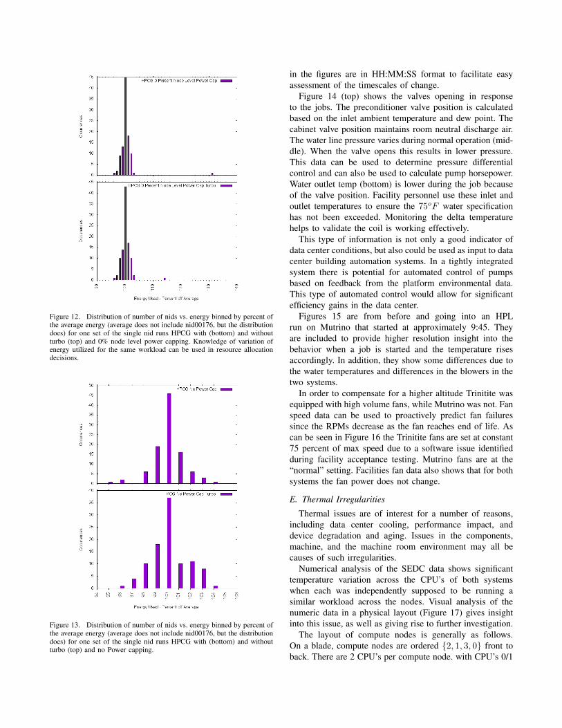
Figure 12. Distribution of number of nids vs. energy binned by percent ofthe average energy (average does not include nid00176, but the distributiondoes) for one set of the single nid runs HPCG with (bottom) and withoutturbo (top) and 0% node level power capping. Knowledge of variation ofenergy utilized for the same workload can be used in resource allocationdecisions.

Figure 13. Distribution of number of nids vs. energy binned by percent ofthe average energy (average does not include nid00176, but the distributiondoes) for one set of the single nid runs HPCG with (bottom) and withoutturbo (top) and no Power capping.

in the figures are in HH:MM:SS format to facilitate easyassessment of the timescales of change.

Figure 14 (top) shows the valves opening in responseto the jobs. The preconditioner valve position is calculatedbased on the inlet ambient temperature and dew point. Thecabinet valve position maintains room neutral discharge air.The water line pressure varies during normal operation (mid-dle). When the valve opens this results in lower pressure.This data can be used to determine pressure differentialcontrol and can also be used to calculate pump horsepower.Water outlet temp (bottom) is lower during the job becauseof the valve position. Facility personnel use these inlet andoutlet temperatures to ensure the 75oF water specificationhas not been exceeded. Monitoring the delta temperaturehelps to validate the coil is working effectively.

This type of information is not only a good indicator ofdata center conditions, but also could be used as input to datacenter building automation systems. In a tightly integratedsystem there is potential for automated control of pumpsbased on feedback from the platform environmental data.This type of automated control would allow for significantefficiency gains in the data center.

Figures 15 are from before and going into an HPLrun on Mutrino that started at approximately 9:45. Theyare included to provide higher resolution insight into thebehavior when a job is started and the temperature risesaccordingly. In addition, they show some differences due tothe water temperatures and differences in the blowers in thetwo systems.

In order to compensate for a higher altitude Trinitite wasequipped with high volume fans, while Mutrino was not. Fanspeed data can be used to proactively predict fan failuressince the RPMs decrease as the fan reaches end of life. Ascan be seen in Figure 16 the Trinitite fans are set at constant75 percent of max speed due to a software issue identifiedduring facility acceptance testing. Mutrino fans are at the“normal” setting. Facilities fan data also shows that for bothsystems the fan power does not change.

E. Thermal Irregularities

Thermal issues are of interest for a number of reasons,including data center cooling, performance impact, anddevice degradation and aging. Issues in the components,machine, and the machine room environment may all becauses of such irregularities.

Numerical analysis of the SEDC data shows significanttemperature variation across the CPU’s of both systemswhen each was independently supposed to be running asimilar workload across the nodes. Visual analysis of thenumeric data in a physical layout (Figure 17) gives insightinto this issue, as well as giving rise to further investigation.

The layout of compute nodes is generally as follows.On a blade, compute nodes are ordered {2, 1, 3, 0} front toback. There are 2 CPU’s per compute node. with CPU’s 0/1

Figure 14. Trinitite machine data over the Series: Flow Rates andValves (top) (Preconditioner water valve position is always 0.), Water LinePressures (middle), Water Outlet Temp (bottom). We seek understandingof the response of the machine to workloads to enable automated controlof the facilities as a whole.

Figure 15. Mutrino data for comparison, going into an HPL run thatstarted at approximately 9:45. Flow Rates and Valves (top), Water LinePressures (middle), Water Outlet Temp (bottom).

Figure 16. Blower Speed: Trinitite data over the Series (top). Mutrinogoing into an HPL run (bottom).

alternating left/right with each node. There are two servicenodes per blade. Within the rack, chassis are verticallystacked. Two slots can be populated left and right in achassis.

Figure 17 shows the layout for the two machines (Trinitite(top), Mutrino (bottom)). Slots with Service Nodes arelocated on the bottom left slots of each chassis; diffuser slotsare located at the tops of the chassis; either are indicated bythe small blue dots (color not indicative of temperature fornon-compute nodes).

Maximum CPU temperatures for each compute node overthe workload for each case are shown, with the exception ofTrinitite’s c0-0c2s12n0, as discussed below. The workloadswere not the same for each machine. For Trinitite, theworkload was the entire set of runs discussed in this work(3 Series). For Mutrino, the workload was the entire HPLrun (approx 3 hours) pertaining to the Mutrino figures inSection V-D. While it is not expected for the values to becomparable, certain similarities occur in both.

Figure 17. Thermal distributions on Trinitite (top) and Mutrino (bottom)shown in the layout of the rack (not to scale). Air flows left to right. Thereis significant temperature variation across the system and across CPUs ona slot. Temperatures are markedly higher when the left and right slots areboth populated (overlap rows labeled in top figure). c0-0c2s12n0/nid00176is of interest in both systems.

There is a significant overall variation in CPU temperature(25-30oC). These large differences could lead to differencesin component aging, performance, and failure rates. Inaddition, there can be a greater than 10oC temperaturevariation across CPUs in the same blade. In general, thehotter nodes are seen to be those for which the left and rightslots are both populated. In addition, c0-0c2s12n0, whichis nid00176, has issues in both systems: in Mutrino thisnode has been exhibiting temperature related throttling; in

Trinitite the SEDC data included error codes for all attemptsat collecting temperature related data for this run and inthe log data this nid was the only nid reporting an errorwhen attempting to apply the power capping profiles. Afterfurther discussion with Cray [14], we believe these Trinititeissues may be related as the same communications channelis used to issue the power capping command and to obtainthe SEDC data. As of this writing, the occurrence of thiscommunications failure remains unresolved. We do not haveenough information to determine if the situation might bethermally related.

As a result we seek further understanding of the commonpositional dependence of the problem nid, of the overallexpectations of temperature within the partially populatedracks, and of how we can expect the results to extrapolateto fully populated systems.

F. Network

While the workload did not target investigation of net-work performance and Aries environmental data profiling,the Aries does consume energy and understanding whencontention for network resources (congestion) is affectingperformance can aid in root cause analysis of performancevariability and help in optimization of job placement thatminimizes congestion. We briefly present a first look at thisdata in the form of link bandwidth used and associated stalls(a measure of congestion).

Figure 18 plots network traffic (top) and stalls (middle)data for each of the 40 outward facing Aries router tiles.This data was gathered from the gpcdr interface via LDMS(Section III-D) during the course of the same applicationruns previously presented. As expected there are no trafficor stall values during the single node jobs and highestvalues occur during the 100 node combustion code run.(Only the times in the first set of runs in the Series (non-turbo) are marked.) The bottom figure shows related SEDCenvironmental data on the Aries associated with the entireblade associated with that node. Note all nodes of a bladeshare an Aries router and the data shown here, thoughcollected by one node, is for all traffic and stalls associatedits Aries router. For this workload, there is only a slight, butnoticeable, effect on the current (bottom) during the runs.Future work involves consideration of more communicationintensive workloads.

VI. CONCLUSIONS AND FUTURE WORK

Integration of data from a variety of sources is necessaryfor system understanding, improving system performance,and problem diagnosis. This becomes increasingly necessaryas we continue to push the boundaries of the data centerinfrastructure supporting HPC systems.

In this paper we have considered information integrationand analysis functionalities currently deployed and underdevelopment on the ACES ART systems for Trinity. Data

Figure 18. Integrating Network traffic and environmental data. Traffic(top), stalls (middle) collected on an arbitrary nid during the no cappingcase. Aries SEDC values for the slot of that same nid (bottom).

sources include facilities, machine, and node level data andinclude both numeric and log data types. Our monitoringarchitecture is intended to support run-time analysis anddecision-making based on the data. We presented actualcases of analysis of the integrated data relating to power,cooling, and thermal issues and areas of interest. In partic-ular, as we have targeted enabling more advanced facilitiesoperation, our integration and analysis of this data has beenkey in identifying the need for a more clear understandingof the differences between machine and data center powerreporting.

Future work includes the deployment of these monitoringcapabilities on Trinity and further analysis and understand-ing of system behaviors and abnormalities particularly asthey relate to power, thermal, and networking issues. Weseek to capture metrics from the platform which can thendrive infrastructure efficiencies through automating dynamicfacility control. We seek to enable capabilties such aspower capping and load shedding from the platform torespond to facility power and cooling constraints. We planto characterize behaviors in order to predict optimal curveratios from pump and tower perspectives. We will analyzeratios of power usage of components within compute hosts(power supplies, DIMMS, and CPUs) in order to drivemore specifications for more efficient architectures in futureprocurements. Ultimately, our long term goal is to useour enhanced understanding to enable advanced operationsof the site facilities in concert with the site’s machinesoperations.

ACKNOWLEDGMENTS

The authors would like to thank Jason Repik (Cray) forconfiguration, advice, and diagnostics; Paul Casella (Cray)for information and fixes to Cray’s gpcdr module; Joshi Ful-lop (NCSA) and Victor Kuhns (Cray) for useful discussionson the forwarding of SEDC and log data; Adam DeCon-inck (LANL), Kathleen Kelly (LANL), and Jim Williams(LANL) who administer the platforms and facilitated theruns used in this work. and Alynna Montoya-Wuiff (LANL)and Eloy Romero (LANL) for access to facilities data.

REFERENCES

[1] J. Kim, W. J. Dally, S. Scott, and D. Abts,“Technology-driven, highly-scalable dragonfly topology,”SIGARCH Comput. Archit. News, vol. 36, no. 3,pp. 77–88, Jun. 2008. [Online]. Available: http://doi.acm.org/10.1145/1394608.1382129

[2] “Using and Configuring System Environment DataCollections (SEDC) Cray Doc S-2491-7001,” 2012.[Online]. Available: http://docs.cray.com/books/S-2491-7001/S-2491-7001.pdf

[3] P. Falde, private communication.

[4] J. Laros, D. DeBonis, R. Grant, S. Kelly, M. Levenhagen,S. Olivier, and K. Pedretti, “High Performance Computing -Power Application Programming INterface Specification, Ver-sion 1.0,” Sandia National Laboratories, Albuquerque, NewMexico 87185 and Livermore, California 94550, Technicalreport SAND2014-17061, 2014.

[5] “Monitoring and Managing Power Consumption onthe Cray XC System Cray Doc S-0043-7202,” 2014.[Online]. Available: http://docs.cray.com/books/S-0043-7202/S-0043-7202.pdf

[6] A. Agelastos, B. Allan, J. Brandt, P. Cassella, J. Enos,J. Fullop, A. Gentile, S. Monk, N. Naksinehaboon, J. Ogden,M. Rajan, M. Showerman, J. Stevenson, N. Taerat, andT. Tucker, “Lightweight Distributed Metric Service: A Scal-able Infrastructure for Continuous Monitoring of Large ScaleComputing Systems and Applications,” in Proc. IEEE/ACMInternational Conference for High Performance Storage, Net-working, and Analysis (SC14), 2014.

[7] P. Cassella, private communication.

[8] “Trane.” [Online]. Available: http://trane.com

[9] C. McMurtrie, L. Gilly, and T. Belotti, “Cray Hybrid XC30Installation - Facilities Level Overview,” in Cray User’sGroup, 2014.

[10] “HPL.” [Online]. Available: http://www.netlib.org/benchmark/hpl/

[11] “HPCG.” [Online]. Available: http://www.hpcg-benchmark.org

[12] “HPCG Performance.” [Online]. Available: https://software.sandia.gov/hpcg/2014-06-hpcg-list.pdf

[13] N. Taerat, J. Brandt, A. Gentile, M. Wong, andC. Leangsuksun, “Baler: deterministic, lossless log messageclustering tool,” Computer Science - Research andDevelopment, vol. 26, no. 3-4, pp. 285–295, 2011. [Online].Available: http://dx.doi.org/10.1007/s00450-011-0155-3

[14] S. Martin and D. Rush, private communication.