enabling dynamic voltage and frequency scaling in multicore architectures€¦ · ·...
TRANSCRIPT
Enabling Dynamic Voltage and Frequency Scaling in
Multicore Architectures
by
Amithash Prasad
B.S., Visveswaraya Technical University, 2005
A thesis submitted to the
Faculty of the Graduate School of the
University of Colorado in partial fulfillment
of the requirements for the degree of
Master of Science
Department of Electrical and Computer Engineering
2009
This thesis entitled:Enabling Dynamic Voltage and Frequency Scaling in Multicore Architectures
written by Amithash Prasadhas been approved for the Department of Electrical and Computer Engineering
Prof. Dan Connors (chair)
Prof. Manish Vachharajani
Date
The final copy of this thesis has been examined by the signatories, and we find that both thecontent and the form meet acceptable presentation standards of scholarly work in the above
mentioned discipline.

iii
Prasad, Amithash (M.S., Electrical Engineering)
Enabling Dynamic Voltage and Frequency Scaling in Multicore Architectures
Thesis directed by Prof. Dan Connors (chair)
Traditional operating system methodologies in controlling the voltage and frequency
configuration of the machine are mostly based on ad-hoc means, thermal emergencies or con-
straining the power consumption of the system. Issues such as low memory latency, cache shar-
ing, depleting memory bandwidth have for long hindered clock speed scaling. Higher clock
speed no longer indicate better performance.
This thesis presents a scheduling methodology for multicore processors which maps run-
ning applications to cores executing at varied clock speeds based on their runtime performance
characteristic. Two schemes of mapping tasks to cores were designed. An asynchronously run
power optimizer was devised to adapt to the needs of the current workload in terms of core
clock speed on a multicore system accomplished by utilizing the information provided by the
scheduler about the needs of the current workload. The entire system was implemented as a
module for the Linux kernel.
In addition to these contributions, this thesis performs an extensive analysis on the system
for six selected workloads to analyze the effects on performance, power and energy efficiency.
Additionally this thesis presents future possible applications of the developed infrastructure
to aid compiler and user-space runtime designers to utilize the framework and provide useful
information about task characteristic and phase behavior to the operating system scheduler for
better task to clock speed assignments.

Dedication
This thesis is dedicated to my fiance Sushma for listening to me whine during the initial part of
this thesis when whatever I touched seemed to crash; For listening to me gloat in pride when
things worked for a change, and finally for proof reading my thesis when I realized that I have
forgotten the entire English language.

v
Acknowledgements
There is a saying in Sanskrit guru devo bavaha roughly translating to A professor is
equivalent to god. Thus I would like to begin my acknowledgement by thanking those who
have imparted me the most important wealth: knowledge.
First, I would like to thank my advisers Dan Connors and Manish Vachharajani for their
advice, tutoring, and incredible patience. I am grateful for the courses they taught which got
me interested in computer engineering and lured me away from control systems which was my
initial idea of a master’s degree.
Second, I’d like to thank Professor Dirk Grunwald for his motivation and suggestions
every time I stumbled into his office without an appointment which shows the level of his
patience and the willingness to help.
Third, I’d like to thank Tipp Moseley a fellow graduate student for helping me out during
my initial introduction into kernel hacking, and answering my questions whenever I felt that I
was somehow within the grasp of a black hole. This does not exclude the very helpful and
friendly Linux kernel community who helped a novice transition into a real kernel hacker. This
would not end without thanking Linus Torvalds for creating the Linux kernel in the first place.
Finally, I’d like to thank my parents for motivating me all along, understanding when I
barely call them and to have faith in me and all my endeavors (no matter how foolish it might
sound).
vi
Contents
Chapter
1 Introduction 1
2 Impact of clock speed scaling on application performance 4
2.1 Performance behavior of SPEC workloads . . . . . . . . . . . . . . . . . . . . 4
2.2 Quantifying performance . . . . . . . . . . . . . . . . . . . . . . . . . . . . . 7
3 Performance directed scheduling on multicore processors 10
3.1 Hierarchical processor organization . . . . . . . . . . . . . . . . . . . . . . . 11
3.2 Hardware performance counters . . . . . . . . . . . . . . . . . . . . . . . . . 11
3.3 Scheduling methodology . . . . . . . . . . . . . . . . . . . . . . . . . . . . . 13
3.3.1 Performance state estimation with the Ladder approach (LEA) . . . . . 14
3.3.2 Performance state estimation with the select approach (SEA) . . . . . . 15
3.4 Experimental setup . . . . . . . . . . . . . . . . . . . . . . . . . . . . . . . . 16
3.5 Static/Fixed layout of processor cores . . . . . . . . . . . . . . . . . . . . . . 17
4 Power-aware throughput management on multicore systems 19
4.1 Common power management systems . . . . . . . . . . . . . . . . . . . . . . 20
4.2 Overview of the Linux cpufreq architecture . . . . . . . . . . . . . . . . . . . 21
4.3 Proposed system overview . . . . . . . . . . . . . . . . . . . . . . . . . . . . 22
4.4 Problem definition . . . . . . . . . . . . . . . . . . . . . . . . . . . . . . . . 25
vii
4.5 The delta constrained mutation algorithm . . . . . . . . . . . . . . . . . . . . 27
4.5.1 Initialization . . . . . . . . . . . . . . . . . . . . . . . . . . . . . . . 28
4.5.2 The Manhattan matrix . . . . . . . . . . . . . . . . . . . . . . . . . . 30
4.5.3 The Manhattan weight vector . . . . . . . . . . . . . . . . . . . . . . 34
4.5.4 Cooperative demand distribution: The demand field . . . . . . . . . . . 34
4.5.5 Greedy performance state selection . . . . . . . . . . . . . . . . . . . 35
4.5.6 Greedy processor selection and transition . . . . . . . . . . . . . . . . 36
4.5.7 Parameter change and termination conditions . . . . . . . . . . . . . . 36
5 Experimental setup and results 38
5.1 Trends along delta and interval . . . . . . . . . . . . . . . . . . . . . . . . . . 40
5.2 Trends along maximum allowed mutation rate . . . . . . . . . . . . . . . . . . 43
5.3 Comparing various methodologies and varying workloads . . . . . . . . . . . . 45
6 Future work 50
7 Summary and Conclusion 51
Bibliography 53
Appendix
A AMD Opteron capabilities 56
B Mutation time-line per workload 57
C Source code 61
viii
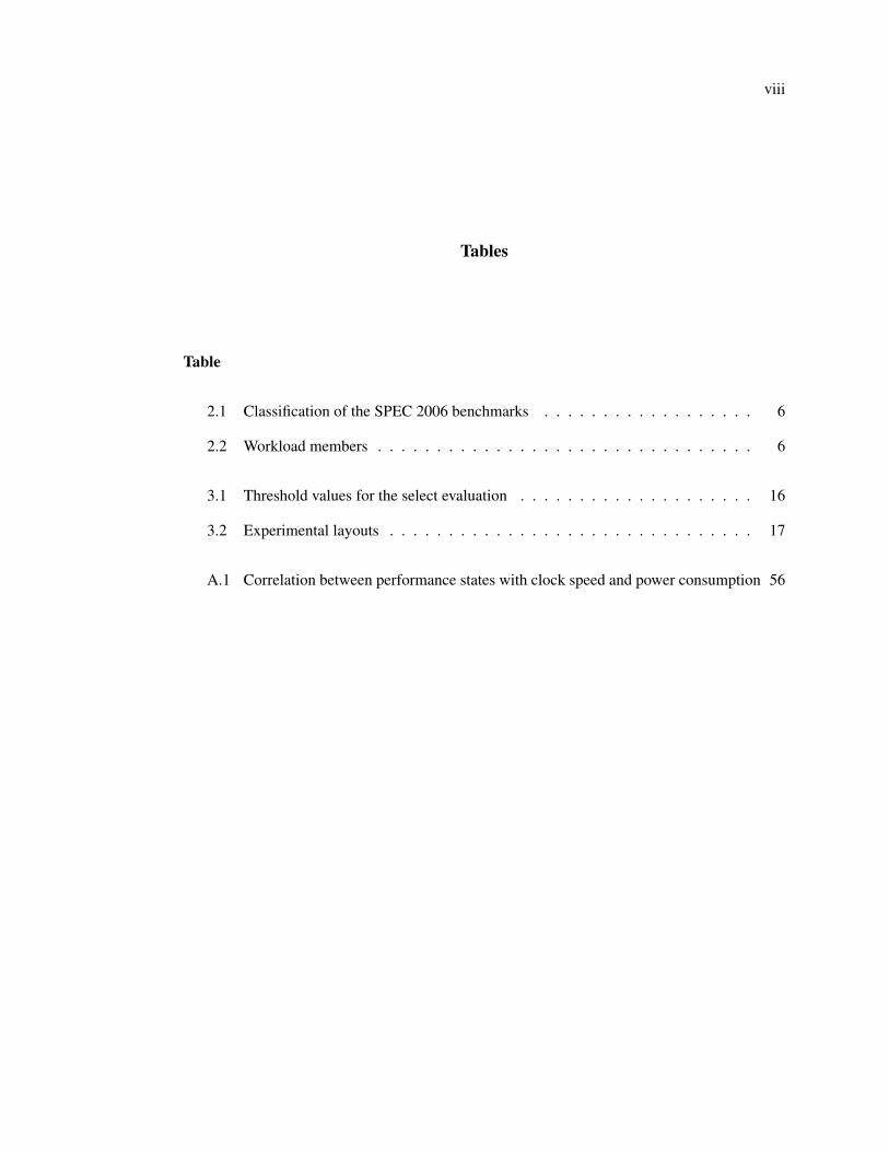
Tables
Table
2.1 Classification of the SPEC 2006 benchmarks . . . . . . . . . . . . . . . . . . 6
2.2 Workload members . . . . . . . . . . . . . . . . . . . . . . . . . . . . . . . . 6
3.1 Threshold values for the select evaluation . . . . . . . . . . . . . . . . . . . . 16
3.2 Experimental layouts . . . . . . . . . . . . . . . . . . . . . . . . . . . . . . . 17
A.1 Correlation between performance states with clock speed and power consumption 56
ix
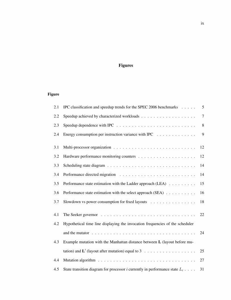
Figures
Figure
2.1 IPC classification and speedup trends for the SPEC 2006 benchmarks . . . . . 5
2.2 Speedup achieved by characterized workloads . . . . . . . . . . . . . . . . . . 7
2.3 Speedup dependence with IPC . . . . . . . . . . . . . . . . . . . . . . . . . . 8
2.4 Energy consumption per instruction variance with IPC . . . . . . . . . . . . . 9
3.1 Multi-processor organization . . . . . . . . . . . . . . . . . . . . . . . . . . . 12
3.2 Hardware performance monitoring counters . . . . . . . . . . . . . . . . . . . 12
3.3 Scheduling state diagram . . . . . . . . . . . . . . . . . . . . . . . . . . . . . 14
3.4 Performance directed migration . . . . . . . . . . . . . . . . . . . . . . . . . 14
3.5 Performance state estimation with the Ladder approach (LEA) . . . . . . . . . 15
3.6 Performance state estimation with the select approach (SEA) . . . . . . . . . . 16
3.7 Slowdown vs power consumption for fixed layouts . . . . . . . . . . . . . . . 18
4.1 The Seeker governor . . . . . . . . . . . . . . . . . . . . . . . . . . . . . . . 22
4.2 Hypothetical time line displaying the invocation frequencies of the scheduler
and the mutator . . . . . . . . . . . . . . . . . . . . . . . . . . . . . . . . . . 24
4.3 Example mutation with the Manhattan distance between L (layout before mu-
tation) and L′ (layout after mutation) equal to 3 . . . . . . . . . . . . . . . . . 25
4.4 Mutation algorithm . . . . . . . . . . . . . . . . . . . . . . . . . . . . . . . . 27
4.5 State transition diagram for processor i currently in performance state Li . . . . 31
x
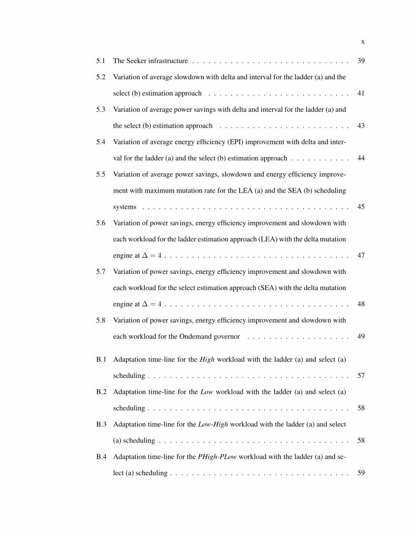
5.1 The Seeker infrastructure . . . . . . . . . . . . . . . . . . . . . . . . . . . . . 39
5.2 Variation of average slowdown with delta and interval for the ladder (a) and the
select (b) estimation approach . . . . . . . . . . . . . . . . . . . . . . . . . . 41
5.3 Variation of average power savings with delta and interval for the ladder (a) and
the select (b) estimation approach . . . . . . . . . . . . . . . . . . . . . . . . 43
5.4 Variation of average energy efficiency (EPI) improvement with delta and inter-
val for the ladder (a) and the select (b) estimation approach . . . . . . . . . . . 44
5.5 Variation of average power savings, slowdown and energy efficiency improve-
ment with maximum mutation rate for the LEA (a) and the SEA (b) scheduling
systems . . . . . . . . . . . . . . . . . . . . . . . . . . . . . . . . . . . . . . 45
5.6 Variation of power savings, energy efficiency improvement and slowdown with
each workload for the ladder estimation approach (LEA) with the delta mutation
engine at ∆ = 4 . . . . . . . . . . . . . . . . . . . . . . . . . . . . . . . . . . 47
5.7 Variation of power savings, energy efficiency improvement and slowdown with
each workload for the select estimation approach (SEA) with the delta mutation
engine at ∆ = 4 . . . . . . . . . . . . . . . . . . . . . . . . . . . . . . . . . . 48
5.8 Variation of power savings, energy efficiency improvement and slowdown with
each workload for the Ondemand governor . . . . . . . . . . . . . . . . . . . 49
B.1 Adaptation time-line for the High workload with the ladder (a) and select (a)
scheduling . . . . . . . . . . . . . . . . . . . . . . . . . . . . . . . . . . . . . 57
B.2 Adaptation time-line for the Low workload with the ladder (a) and select (a)
scheduling . . . . . . . . . . . . . . . . . . . . . . . . . . . . . . . . . . . . . 58
B.3 Adaptation time-line for the Low-High workload with the ladder (a) and select
(a) scheduling . . . . . . . . . . . . . . . . . . . . . . . . . . . . . . . . . . . 58
B.4 Adaptation time-line for the PHigh-PLow workload with the ladder (a) and se-
lect (a) scheduling . . . . . . . . . . . . . . . . . . . . . . . . . . . . . . . . . 59

xi
B.5 Adaptation time-line for the PLow-Low workload with the ladder (a) and select
(a) scheduling . . . . . . . . . . . . . . . . . . . . . . . . . . . . . . . . . . . 59
B.6 Adaptation time-line for the PLow-High workload with the ladder (a) and select
(a) scheduling . . . . . . . . . . . . . . . . . . . . . . . . . . . . . . . . . . . 60
Chapter 1
Introduction
Emerging technology constraints are slowing the rate of performance growth in com-
puter systems. Specifically, designers are finding difficulties addressing strict processor power
consumption and cooling constraints. Design modifications to address power consumption gen-
erally limit processor performance and reduce peak operating frequency, thus changing the
trend of providing increased system performance every new processor generation. As such,
modern architectures have diverged from the clock speed race into the multicore era with mul-
tiple processing cores on a single chip. While the multicore design strategy improves chip
power density, there remains a significant potential in improving run-time power utilization by
dynamically changing per-core clock frequency and voltage.
Power consumption is directly proportional to the clock speed (frequency) and the square
of the operating voltage of the processor (Power ∝ frequency × V oltage2). In order to con-
serve energy, designers have explored methods to manipulate these parameters using circuit
design techniques and runtime software driven techniques. Implementations of DVFS (Dy-
namic voltage and frequency scaling) schemes divides the processor operation to performance
states or P-states with fixed operating voltage and clock speeds. Architectures supporting mul-
tiple such P-states require active runtime support to fully explore the performance and power
saving potential of the DVFS approach.
The schemes for manipulating DVFS configurations of a processor can be subdivided
2
into three broad categories: Hardware approach [1], [2] and [3] traditionally propose monitor-
ing hardware to predict execution patterns and manipulate the system’s DVFS configuration.
Hardware methods are immutable implementations in silicon which cannot be changed based
on design and policy variations and hence avoided by many chip manufacturers. The second
category is the management of power, controlled by compiler and user space runtime systems
which expect such capabilities to be exported by the operating system as discussed in [4], [5], [6]
and trace driven methods for power management as discussed in [7] and [8]. Operating system
techniques [9], [10], [11] and [12] generally use some of runtime performance monitoring ca-
pabilities exported from the hardware in order to assist in detecting runtime phases, and include
software policies to ultimately make decision for power management.
Majority of DVFS implementations at the operating system level are load based where
the system’s DVFS configuration is varied based upon extremely coarse-grain levels of proces-
sor activity. Even though effective in conserving power such approaches are largely unaware of
the workload currently executing on the system. Load based decisions are best left to technolo-
gies which decide whether the processing element is active or asleep (state at which the power
consumption is minimal) and is studied in [11] which predicts usage patterns of various devices
on the system.
This work proposes techniques which tie the scheduler and the system power optimizer
to constrain the number of DVFS level changes both over time and intensity with the goal of
energy savings without harming individual performance and throughput. Limiting DVFS level
transitions is important to limit instabilities endured by the system due to rapid DVFS transitions
as explored by [13].
This thesis makes the following contributions to this area of study:
(1) Method of scheduling to adjust DVFS with strict constraints on limiting the amount of
performance lost compared to full frequency mode. The system provides significant
power savings of up to 40% with a performance loss of up to 20% with a median

3
performance loss at around 10-15%.
(2) Method to schedule tasks based on their performance requirement on a multi processor
environment with varying per-core clock speeds in order to maximize power savings
while minimizing performance lost.
(3) Investigation of the impact of DVFS level changes per second on the ability to improve
power savings or performance impact.
(4) Design of a multi-task scheduling model that accounts for joule-per-instruction work
metric.
This thesis is organized as follows: Chapter 2 discusses the performance variation of real
world applications with increases in clock speed. Chapter 3 introduces the performance directed
scheduler. Chapter 4 proposes a methodology to mutate voltage and frequency configuration of
a system based on the workload demands. Chapter 5 describes the experimental procedure and
results obtained. Chapter 6 comments on the future work in this area and finally chapter 7
concludes this thesis.
Chapter 2
Impact of clock speed scaling on application performance
Throughput based computing has long been solely dependent on clock speed advantages
for faster application execution. With the onset of multicore processors, a large portion of
research has been devoted to parallelization of sequential applications. The performance of most
real world applications are either dependent on memory speeds or I/O (Input/Output) latency.
Parallel executing threads on a multicore system eventually saturate memory or I/O devices and
thus obtain no advantage of clock speed scaling. This chapter explores the impact of scaling
clock speeds on application performance and energy efficiency in multicore processors.
2.1 Performance behavior of SPEC workloads
In order to study the behavior of real applications on different voltage and frequency
settings, fourteen of the SPEC2006 [14] benchmark suite were run with varied clock speed from
1100 MHz to 2200 MHz on an AMD Opteron quad-core processor and were plotted showing
the percentage duration spent at an IPC (Instruction per Cycle) higher than 1.0 and the speed-up
in terms of execution time achieved from that when run with the lowest clock speed (1100 MHz)
shown in Figure 2.1. The X-axis of this graph is the percentage of time the benchmark spent
running at an IPC level greater than 1.0, the Y-axis is the clock speed at which the benchmark
was run at, and finally the Z-axis is the Speed-up achieved. It can be observed that the return
5
on investment (Higher clock speed) is low for tasks with a low percentage of runtime at an IPC
greater than 1.0.
Figure 2.1: IPC classification and speedup trends for the SPEC 2006 benchmarks
The SPEC2006 [14] benchmark suite is a set of real-world applications designed to run
with minimal I/O and hence best used to characterize and study the CPU (central processing
unit) and memory subsystem in modern processors. The applications are typical workloads
used in the field of throughput based computation and is widely used test or design processor
systems. Based on this observation the benchmarks were categorized into four categories: Low,
High, Phased Low and Phased High and shown in Table 2.1.
Table 2.2 shows the breakdown of six workloads (Low, High, Low-High PHigh-PLow,
PLow-High and PLow-Low) comprising of 4 benchmarks each were created (shown in Ta-
ble 2.2) based on their IPC classification in Table 2.1. It must be noted that even though these
workloads were grouped based on their IPC characteristics, it is not uncommon to have work-
loads in the real world comprising of subsets of each benchmarks. The six set of workloads
6Category BenchmarksLow (90%+executes belowand equal toIPC=1.0)
mcf milc libquantum lbm omnetpp
High (90%+executes aboveIPC=1.0)
bzip2 povray hmmer sjeng h264ref
Phased Low(50%+ executesabove IPC=1.0)
gobmk sphinx3
Phased High(50%+ executesbelow and equalto IPC=1.0)
astar xalancbmk
Table 2.1: Classification of the SPEC 2006 benchmarks
provide a fair but experimentally feasible set of applications to estimate the impact of architec-
ture or operating system design.
Workload BenchmarksLow milc libquantum lbm omnetppHigh bzip2 povray hmmer sjengLow-High bzip2 povray milc omnetppPHigh-PLow gobmk sphinx3 astar xalancbmkPLow-High astar xalancbmk povray hmmerPLow-Low astar xalancbmk milc omnetpp
Table 2.2: Workload members
Figure 2.2 shows that the workload High category shows the greatest improvement with
frequency, achieving a nearly 2x improvement using the highest frequency for each core in the
quad-core system. Otherwise, the other categories of workloads appear to benefit from higher
frequency, but are bounded to 1.5x of the baseline execution time. The Low workload is ob-
served to have a very high variance in terms of speedup and shows that clock speeds above 1700
MHz has no effect on the speedup achieved. This motivates the construction of a performance
directed scheduler aware of the IPC level at which tasks are executing and described in further
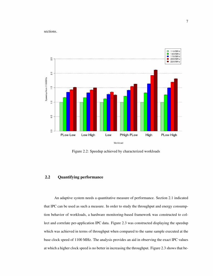
7
sections.
Figure 2.2: Speedup achieved by characterized workloads
2.2 Quantifying performance
An adaptive system needs a quantitative measure of performance. Section 2.1 indicated
that IPC can be used as such a measure. In order to study the throughput and energy consump-
tion behavior of workloads, a hardware monitoring-based framework was constructed to col-
lect and correlate per-application IPC data. Figure 2.3 was constructed displaying the speedup
which was achieved in terms of throughput when compared to the same sample executed at the
base clock speed of 1100 MHz. The analysis provides an aid in observing the exact IPC values
at which a higher clock speed is no better in increasing the throughput. Figure 2.3 shows that be-
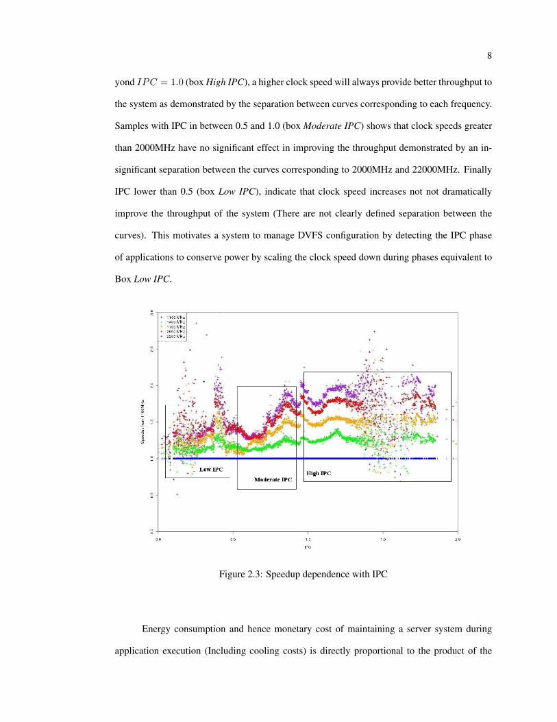
8
yond IPC = 1.0 (box High IPC), a higher clock speed will always provide better throughput to
the system as demonstrated by the separation between curves corresponding to each frequency.
Samples with IPC in between 0.5 and 1.0 (box Moderate IPC) shows that clock speeds greater
than 2000MHz have no significant effect in improving the throughput demonstrated by an in-
significant separation between the curves corresponding to 2000MHz and 22000MHz. Finally
IPC lower than 0.5 (box Low IPC), indicate that clock speed increases not not dramatically
improve the throughput of the system (There are not clearly defined separation between the
curves). This motivates a system to manage DVFS configuration by detecting the IPC phase
of applications to conserve power by scaling the clock speed down during phases equivalent to
Box Low IPC.
Figure 2.3: Speedup dependence with IPC
Energy consumption and hence monetary cost of maintaining a server system during
application execution (Including cooling costs) is directly proportional to the product of the
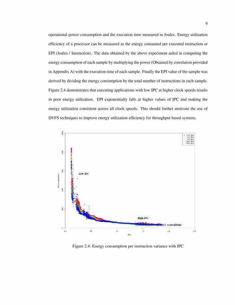
9
operational power consumption and the execution time measured in Joules. Energy utilization
efficiency of a processor can be measured as the energy consumed per executed instruction or
EPI (Joules / Instruction). The data obtained by the above experiment aided in computing the
energy consumption of each sample by multiplying the power (Obtained by correlation provided
in Appendix A) with the execution time of each sample. Finally the EPI value of the sample was
derived by dividing the energy consumption by the total number of instructions in each sample.
Figure 2.4 demonstrates that executing applications with low IPC at higher clock speeds results
in poor energy utilization. EPI exponentially falls at higher values of IPC and making the
energy utilization consistent across all clock speeds. This should further motivate the use of
DVFS techniques to improve energy utilization efficiency for throughput based systems.
Figure 2.4: Energy consumption per instruction variance with IPC
Chapter 3
Performance directed scheduling on multicore processors
Current implementations of schedulers in modern operating systems recognize the en-
vironment as homogeneous in nature while technologies such as DVFS introduce an inherent
asymmetry in a multicore system. Considerable exploration in terms of asymmetric scheduling
support has been investigated in [15] and [16]. However, the work ignores the fact that certain
workloads do not gain sufficient advantages from increased clock speeds discovered in Chap-
ter 2 which could assist in conserving power by scaling the clock speed down during phases of
low IPC.
In a multicore environment, there are many facets for performance loss with the most
common reasons being high IO and memory latencies which is further aggravated by cache
sharing. A novel statistical learning method to predict voltage and frequency requirements by
tasks was proposed in [5], but the method required rigorous statistical learning making it time
consuming and impossible to implement at the context of a scheduler. For example even with a
quad core system and a scheduling frequency of 1000Hz, there is a possibility of 1000 × 4 =
4000 performance state transitions every second which can cause instabilities as shown in [13].
A simpler method was proposed in [10] and [2], but comes at the cost of possible rapid voltage
and frequency transitions which may lead to instabilities in emergencies
11
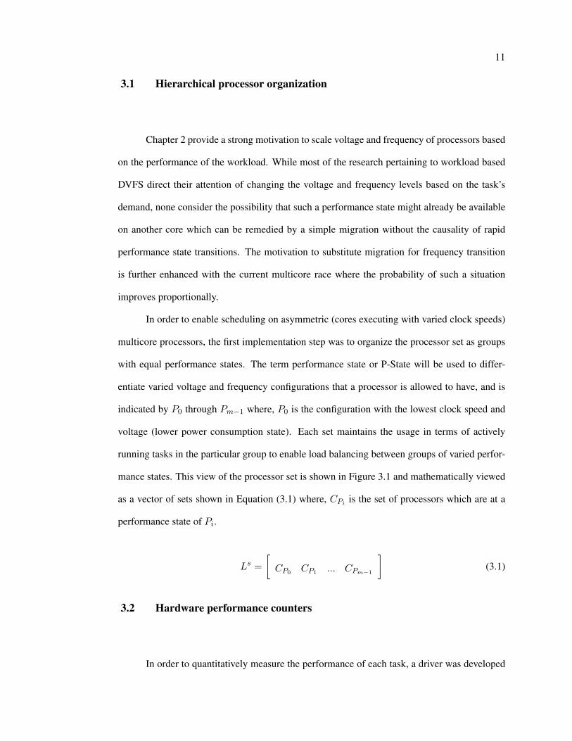
3.1 Hierarchical processor organization
Chapter 2 provide a strong motivation to scale voltage and frequency of processors based
on the performance of the workload. While most of the research pertaining to workload based
DVFS direct their attention of changing the voltage and frequency levels based on the task’s
demand, none consider the possibility that such a performance state might already be available
on another core which can be remedied by a simple migration without the causality of rapid
performance state transitions. The motivation to substitute migration for frequency transition
is further enhanced with the current multicore race where the probability of such a situation
improves proportionally.
In order to enable scheduling on asymmetric (cores executing with varied clock speeds)
multicore processors, the first implementation step was to organize the processor set as groups
with equal performance states. The term performance state or P-State will be used to differ-
entiate varied voltage and frequency configurations that a processor is allowed to have, and is
indicated by P0 through Pm−1 where, P0 is the configuration with the lowest clock speed and
voltage (lower power consumption state). Each set maintains the usage in terms of actively
running tasks in the particular group to enable load balancing between groups of varied perfor-
mance states. This view of the processor set is shown in Figure 3.1 and mathematically viewed
as a vector of sets shown in Equation (3.1) where, CPi is the set of processors which are at a
performance state of Pi.
Ls =[CP0 CP1 ... CPm−1
](3.1)
3.2 Hardware performance counters
In order to quantitatively measure the performance of each task, a driver was developed
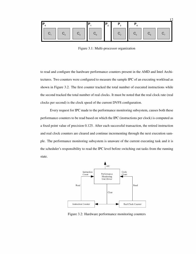
12
Figure 3.1: Multi-processor organization
to read and configure the hardware performance counters present in the AMD and Intel Archi-
tectures. Two counters were configured to measure the sample IPC of an executing workload as
shown in Figure 3.2. The first counter tracked the total number of executed instructions while
the second tracked the total number of real clocks. It must be noted that the real clock rate (real
clocks per second) is the clock speed of the current DVFS configuration.
Every request for IPC made to the performance monitoring subsystem, causes both these
performance counters to be read based on which the IPC (instructions per clock) is computed as
a fixed point value of precision 0.125. After each successful transaction, the retired instruction
and real clock counters are cleared and continue incrementing through the next execution sam-
ple. The performance monitoring subsystem is unaware of the current executing task and it is
the scheduler’s responsibility to read the IPC level before switching out tasks from the running
state.
Figure 3.2: Hardware performance monitoring counters
13
3.3 Scheduling methodology
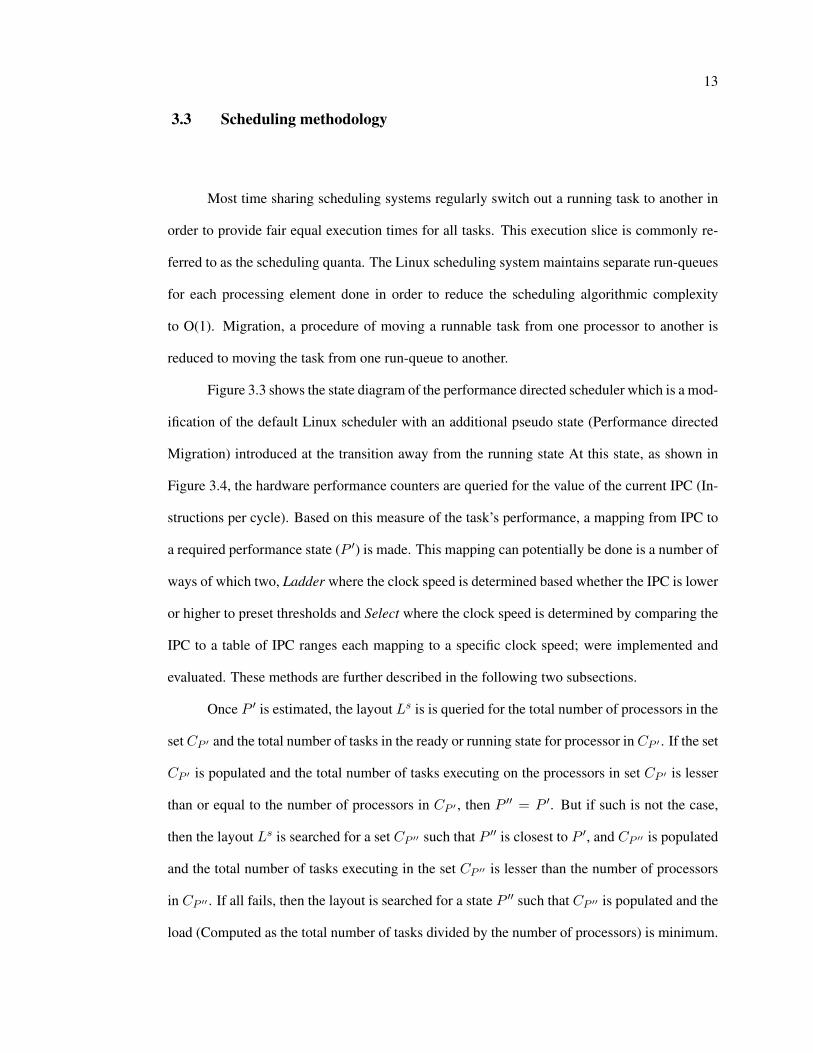
Most time sharing scheduling systems regularly switch out a running task to another in
order to provide fair equal execution times for all tasks. This execution slice is commonly re-
ferred to as the scheduling quanta. The Linux scheduling system maintains separate run-queues
for each processing element done in order to reduce the scheduling algorithmic complexity
to O(1). Migration, a procedure of moving a runnable task from one processor to another is
reduced to moving the task from one run-queue to another.
Figure 3.3 shows the state diagram of the performance directed scheduler which is a mod-
ification of the default Linux scheduler with an additional pseudo state (Performance directed
Migration) introduced at the transition away from the running state At this state, as shown in
Figure 3.4, the hardware performance counters are queried for the value of the current IPC (In-
structions per cycle). Based on this measure of the task’s performance, a mapping from IPC to
a required performance state (P ′) is made. This mapping can potentially be done is a number of
ways of which two, Ladder where the clock speed is determined based whether the IPC is lower
or higher to preset thresholds and Select where the clock speed is determined by comparing the
IPC to a table of IPC ranges each mapping to a specific clock speed; were implemented and
evaluated. These methods are further described in the following two subsections.
Once P ′ is estimated, the layout Ls is is queried for the total number of processors in the
setCP ′ and the total number of tasks in the ready or running state for processor inCP ′ . If the set
CP ′ is populated and the total number of tasks executing on the processors in set CP ′ is lesser
than or equal to the number of processors in CP ′ , then P ′′ = P ′. But if such is not the case,
then the layout Ls is searched for a set CP ′′ such that P ′′ is closest to P ′, and CP ′′ is populated
and the total number of tasks executing in the set CP ′′ is lesser than the number of processors
in CP ′′ . If all fails, then the layout is searched for a state P ′′ such that CP ′′ is populated and the
load (Computed as the total number of tasks divided by the number of processors) is minimum.
14
Finally the task is migrated to the set of processors in CP ′′ . Decisions on the exact processor a
task has to execute on is made by the underlying native scheduler of the operating system and
the PDS is completely oblivious to any further detail. As an interface to the mutator which will
be explained in Chapter 4, PDS increments the cell corresponding to P ′ in the demand vector
D (DP ′ = DP ′ + 1).
Figure 3.3: Scheduling state diagram
Figure 3.4: Performance directed migration
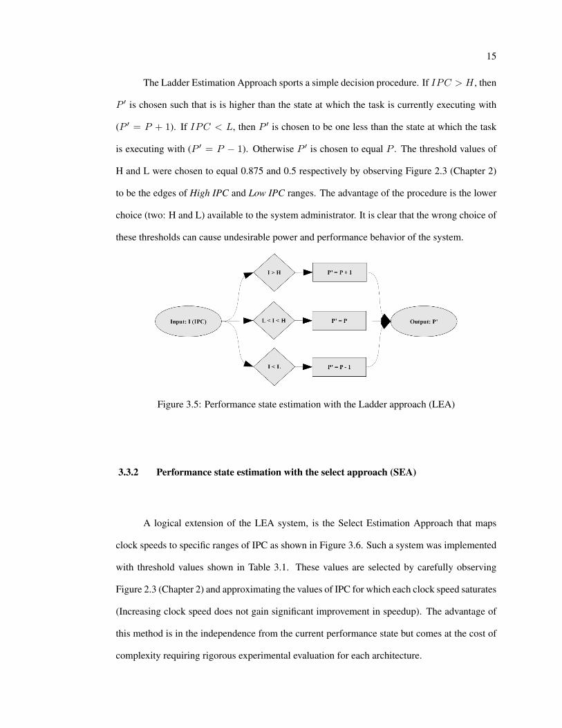
3.3.1 Performance state estimation with the Ladder approach (LEA)
15
The Ladder Estimation Approach sports a simple decision procedure. If IPC > H , then
P ′ is chosen such that is is higher than the state at which the task is currently executing with
(P ′ = P + 1). If IPC < L, then P ′ is chosen to be one less than the state at which the task
is executing with (P ′ = P − 1). Otherwise P ′ is chosen to equal P . The threshold values of
H and L were chosen to equal 0.875 and 0.5 respectively by observing Figure 2.3 (Chapter 2)
to be the edges of High IPC and Low IPC ranges. The advantage of the procedure is the lower
choice (two: H and L) available to the system administrator. It is clear that the wrong choice of
these thresholds can cause undesirable power and performance behavior of the system.
Figure 3.5: Performance state estimation with the Ladder approach (LEA)
3.3.2 Performance state estimation with the select approach (SEA)
A logical extension of the LEA system, is the Select Estimation Approach that maps
clock speeds to specific ranges of IPC as shown in Figure 3.6. Such a system was implemented
with threshold values shown in Table 3.1. These values are selected by carefully observing
Figure 2.3 (Chapter 2) and approximating the values of IPC for which each clock speed saturates
(Increasing clock speed does not gain significant improvement in speedup). The advantage of
this method is in the independence from the current performance state but comes at the cost of
complexity requiring rigorous experimental evaluation for each architecture.

16
Figure 3.6: Performance state estimation with the select approach (SEA)
Threshold ValueT0 0.25T1 0.50T2 0.75T3 1.25
Table 3.1: Threshold values for the select evaluation
A final note of the difference between the LEA and SEA systems: The LEA system
chooses the next higher or lower performance state based on the threshold, while the SEA
system chooses a specific performance state. The SEA and LEA systems were evaluated with
the delta based mutation engine described in Chapter 4.
3.4 Experimental setup
The experiments were conducted on a AMD quad-core Barcelona which allows indi-
vidual processor cores to be set to different clock speeds. The set of workloads described in
Table 2.2, Chapter 2 (groups of SPEC2006 benchmarks) were started on the layouts provided
17
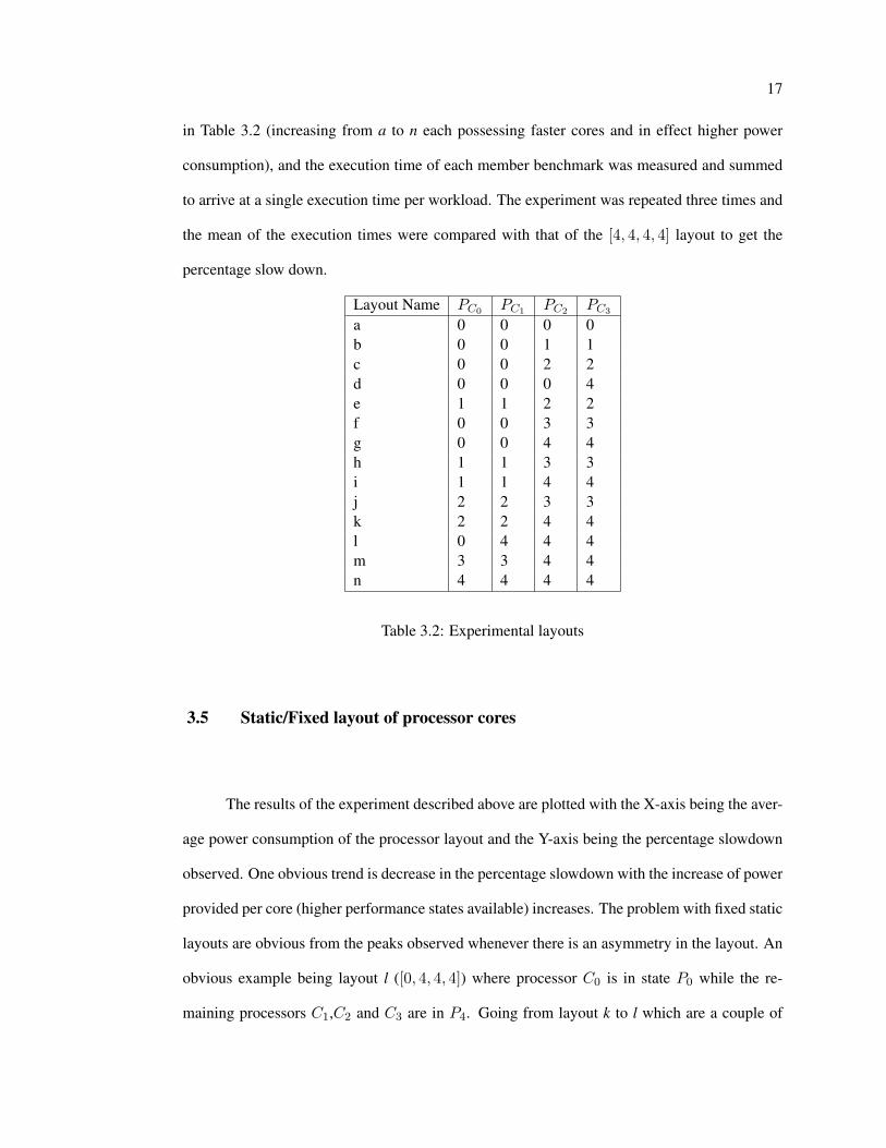
in Table 3.2 (increasing from a to n each possessing faster cores and in effect higher power
consumption), and the execution time of each member benchmark was measured and summed
to arrive at a single execution time per workload. The experiment was repeated three times and
the mean of the execution times were compared with that of the [4, 4, 4, 4] layout to get the
percentage slow down.
Layout Name PC0 PC1 PC2 PC3
a 0 0 0 0b 0 0 1 1c 0 0 2 2d 0 0 0 4e 1 1 2 2f 0 0 3 3g 0 0 4 4h 1 1 3 3i 1 1 4 4j 2 2 3 3k 2 2 4 4l 0 4 4 4m 3 3 4 4n 4 4 4 4
Table 3.2: Experimental layouts
3.5 Static/Fixed layout of processor cores
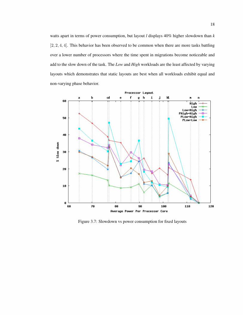
The results of the experiment described above are plotted with the X-axis being the aver-
age power consumption of the processor layout and the Y-axis being the percentage slowdown
observed. One obvious trend is decrease in the percentage slowdown with the increase of power
provided per core (higher performance states available) increases. The problem with fixed static
layouts are obvious from the peaks observed whenever there is an asymmetry in the layout. An
obvious example being layout l ([0, 4, 4, 4]) where processor C0 is in state P0 while the re-
maining processors C1,C2 and C3 are in P4. Going from layout k to l which are a couple of
18
watts apart in terms of power consumption, but layout l displays 40% higher slowdown than k
[2, 2, 4, 4]. This behavior has been observed to be common when there are more tasks battling
over a lower number of processors where the time spent in migrations become noticeable and
add to the slow down of the task. The Low and High workloads are the least affected by varying
layouts which demonstrates that static layouts are best when all workloads exhibit equal and
non-varying phase behavior.
Figure 3.7: Slowdown vs power consumption for fixed layouts

Chapter 4
Power-aware throughput management on multicore systems
Power and energy management are critical to high-performance and high-throughput
environments. Servers are usually limited to the amount of peak power and energy consumed
in order to reduce maintenance cost. As an example, power and energy considerations govern
server space expansion in industries. To combat these constraints, power management systems
are becoming increasingly common in the server space. Two common methodologies exist to
reduce the power consumption of a compute element. The first among which is to turn off
processors during idle time. The second is to keep the system active but lower the operating
frequency and voltage of the processor to utilize proportionally lower power.
In order to fully utilize server nodes and minimize idle time, the current trend among in-
dustries is to run multiple virtual machines on a single server rack thus making varied workloads
common place in an otherwise single purpose server usage. This element further enhances the
requirement of dynamic non-trace driven power management systems. [17] discusses a power
optimizer specialized for a virtual machine farm, but fail to recognize the workload character-
istics of these systems.
Lowering frequency has a pleasant benefit of reducing the power consumption and hence
the energy and cooling costs. But as shown in Chapter 3, Figures 2.3 and 2.4, when the average
IPC of an application is high, reduction in frequency only causes the application to execute for
a proportionally longer duration and hence having no energy benefit (Figure 2.4). The only
20
advantage of reducing the frequency is the reduction of energy supply into the system per unit
time and hence possibly lower heat dissipation.
[5], [10] and [2] propose adapting the clock speed of the processing element based on the
current application’s demand. These methodologies assume that DVFS transitions are local to
that processor core. Some multicore processors have dependency between processor cores (tran-
sitioning one might potentially transition the other) or systems with symmetric multi-threaded
features where a single processor core is visible to the operating system as multiple virtual
processors. Thus, applications executing on such processing elements are tied to each other
and any DVFS transition based on one application might potentially affect another negatively.
Chapter 3 showed that such transitions could be remedied with a simple processor migration
requiring power optimizers to react to the needs of a scheduler.
4.1 Common power management systems
The most popular among power management techniques are load directed systems which
transition a processor to higher or lower performance states based on the current load of the
system. Two of these techniques: ondemand [18] and conservative are implemented within the
thesis infrastructure. The ondemand system raises the performance state to the highest possible
level at high loads, and reduces the performance state gradually to the lowest state during lower
load thus P ′i ,
P ′i =
Pmax : Loadi ≥ 0.8
Pi − 1 : Loadi < 0.8(4.1)
the performance state of processor i after the transition based on the current performance state
Pi and decided based upon load of processor i, loadi. The characteristics of this system is
to rapidly respond to load increase while conservatively lowering the performance state at the
end of the active state. The conservative system, on the other hand, gradually changes the
21
performance state in either direction, where P ′i ,
P ′i =
Pi + 1 : Loadi ≥ 0.8
Pi − 1 : Loadi < 0.8(4.2)
the performance state of processor i, after a transition is decided based on the load of each
processor Loadi with a typical characteristic to gradually meet the system needs and preferred
for servers with typically short running workloads.
4.2 Overview of the Linux cpufreq architecture
In order to maintain architecture independence, separation of methodology and policy,
the subsystem in the Linux kernel responsible for managing the voltage and frequency con-
figuration separates the procedure into two: cpufreq-drivers (The region enclosed by Drivers:
Figure 4.1) are responsible for the actual P-State transition and register with the intermediate
cpufreq layer. cpufreq-governors are responsible for policy and registers with the cpufreq layer.
Policy attributes are:
• How often changes to DVFS configurations are made.
• The magnitude of changes in configuration settings.
Once a working configuration is initialized, the cpufreq-governor instructs the cpufreq-
driver in an indirect fashion on the required transition. As most of the experimentation men-
tioned in this text relates to the AMD Barcelona, the powernow-k8 cpufreq-driver was used to
initiate the transition.
The procedure of changing the DVFS configuration of a multicore processor system is
termed, for the remainder of this thesis, as mutation. The entity involved in making policy
decisions about the nature of the mutation (what processor transitions to what performance
state) is referred to as the mutator. The interval at which mutation decision is performed is
termed the mutation interval.
22
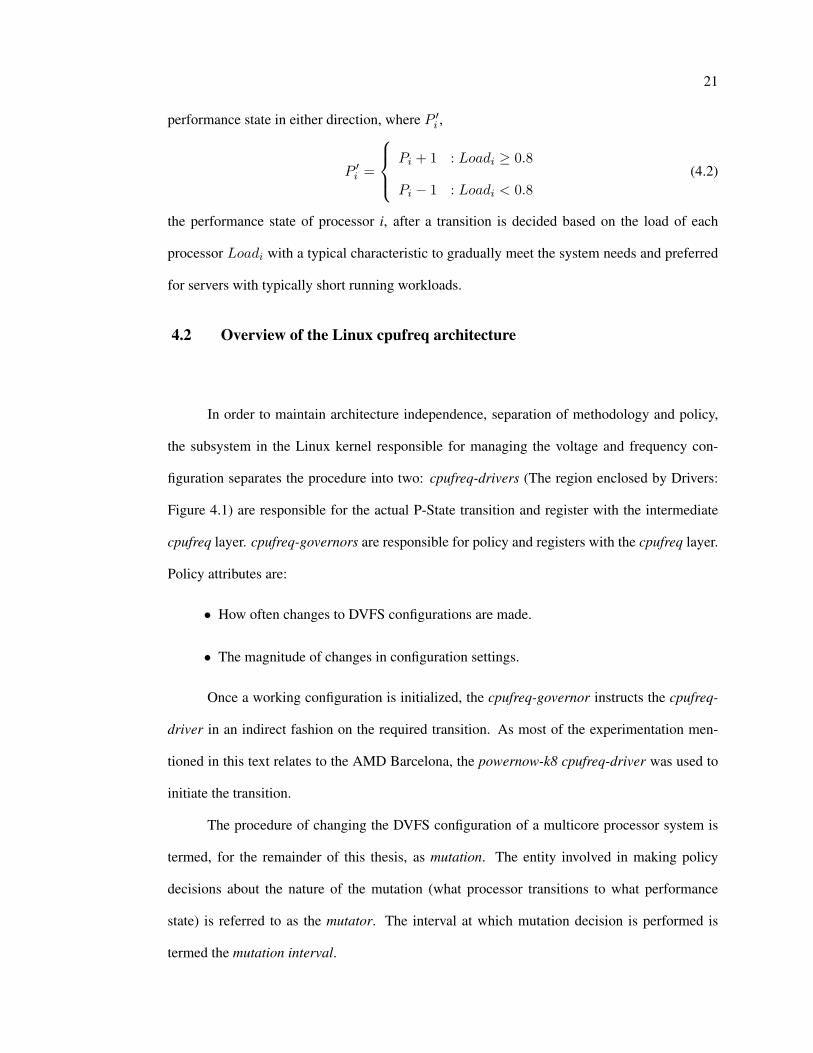
A cpufreq governor seeker was developed having kernel exported interfaces for the mu-
tator to request transitions. A simple registration method was introduced to allow the mutator
to be informed every time a transition is complete as shown in Figure 4.1. The asynchronous
call back mechanism allows the mutator to update its data structures even when an entity other
than itself ( For example, through the sysfs interface) requests for a performance state change.
Figure 4.1: The Seeker governor
4.3 Proposed system overview
In contrast to the load based power management system described in Section 4.1, a
performance directed power management system was implemented. [5], [10] and [2] describe
methodologies where DVFS transitions are invoked based on the performance requirement of
the executing workload of the system. Chapter 3 demonstrated a novel method of substituting
task migrations for DVFS transitions in a multi-processor system where each processor could
23
possible be at varied performance states. With a processor layout Ls being a vector of sets with
a length of m, which allowed the performance directed scheduler to schedule tasks on a set with
an algorithmic complexity of O(m).
Another possible view of the processor layout
Lm = [PC0PC1 ...PCn−1 ] (4.3)
where Lm is a vector of integers of length n, where each element Lmi is the performance state
of processor i. It is clear that both Ls and Lm are different views of the same information
and the proposed mutation scheme must take the responsibility to keep these two views of the
processor layout consistent. As Ls is optimized for the scheduler it will not be further discussed
in this chapter and any reference to processor layout or L will be with respect to the mutation
engine’s view of the processor layout: Lm. Thus the processor layout provides n options for
each workload in terms of performance state.
Chapter 3 demonstrated the short comings of a static processor in lieu of varying work-
load in terms of characteristics and number. In order to alleviate the negative aspects of a static
layout, a mutation scheme was developed allowing the processor layout to adapt on a fixed in-
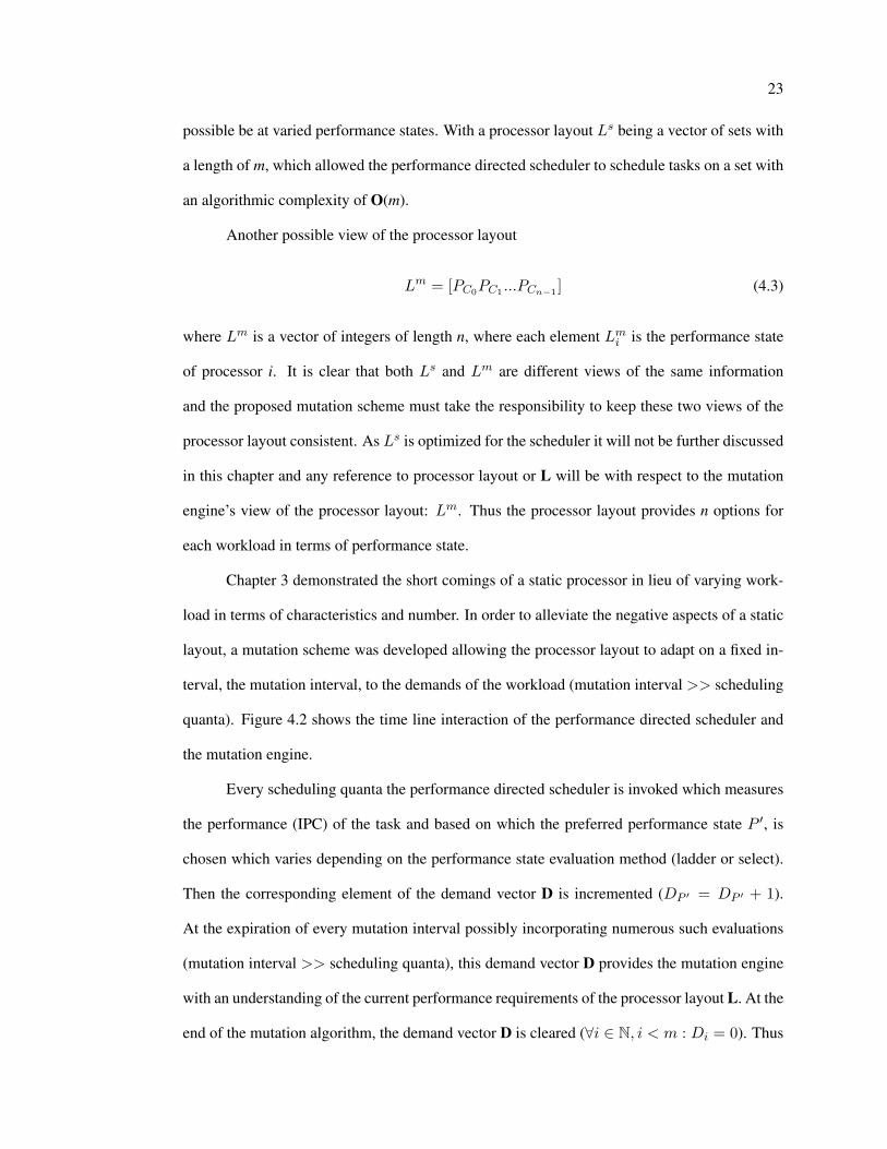
terval, the mutation interval, to the demands of the workload (mutation interval >> scheduling
quanta). Figure 4.2 shows the time line interaction of the performance directed scheduler and
the mutation engine.
Every scheduling quanta the performance directed scheduler is invoked which measures
the performance (IPC) of the task and based on which the preferred performance state P ′, is
chosen which varies depending on the performance state evaluation method (ladder or select).
Then the corresponding element of the demand vector D is incremented (DP ′ = DP ′ + 1).
At the expiration of every mutation interval possibly incorporating numerous such evaluations
(mutation interval >> scheduling quanta), this demand vector D provides the mutation engine
with an understanding of the current performance requirements of the processor layout L. At the
end of the mutation algorithm, the demand vector D is cleared (∀i ∈ N, i < m : Di = 0). Thus
24
Figure 4.2: Hypothetical time line displaying the invocation frequencies of the scheduler andthe mutator
creating an illusion of a dynamic processor layout which adapts to the needs of the machine’s
workload.
Since rapid and drastic DVFS transitions can affect the reliability of the system [13],
operating system management policies are critical. The delta constrained mutation scheme was
developed providing the ability to control the rate of transitions by limiting DVFS transitions
to be performed globally and at fixed interval lengths termed the mutation interval. Secondly,
the delta mutation policy can limit the magnitude of mutation thus eliminating rapid transitions.
The PDS as described in Chapter 3 is performed at the resolution of a scheduler quanta, while
the DVFS transitions are performed at a resolution of the mutation interval and is a multiple
of the scheduling quanta. In order to have an absolute upper bound on the DVFS transitions,
a parameter called the delta constraint (∆) limits the maximum number of mutations that can
be performed at any particular instant (hence limiting the maximum mutations per second to
∆Mutation Interval ).
Delta (∆) for a system with n processors where each processor i is transitioned from
performance state Pi to P ′i can be defined as
∆ ≥n−1∑i=0
|Pi − P ′i | (4.4)
25
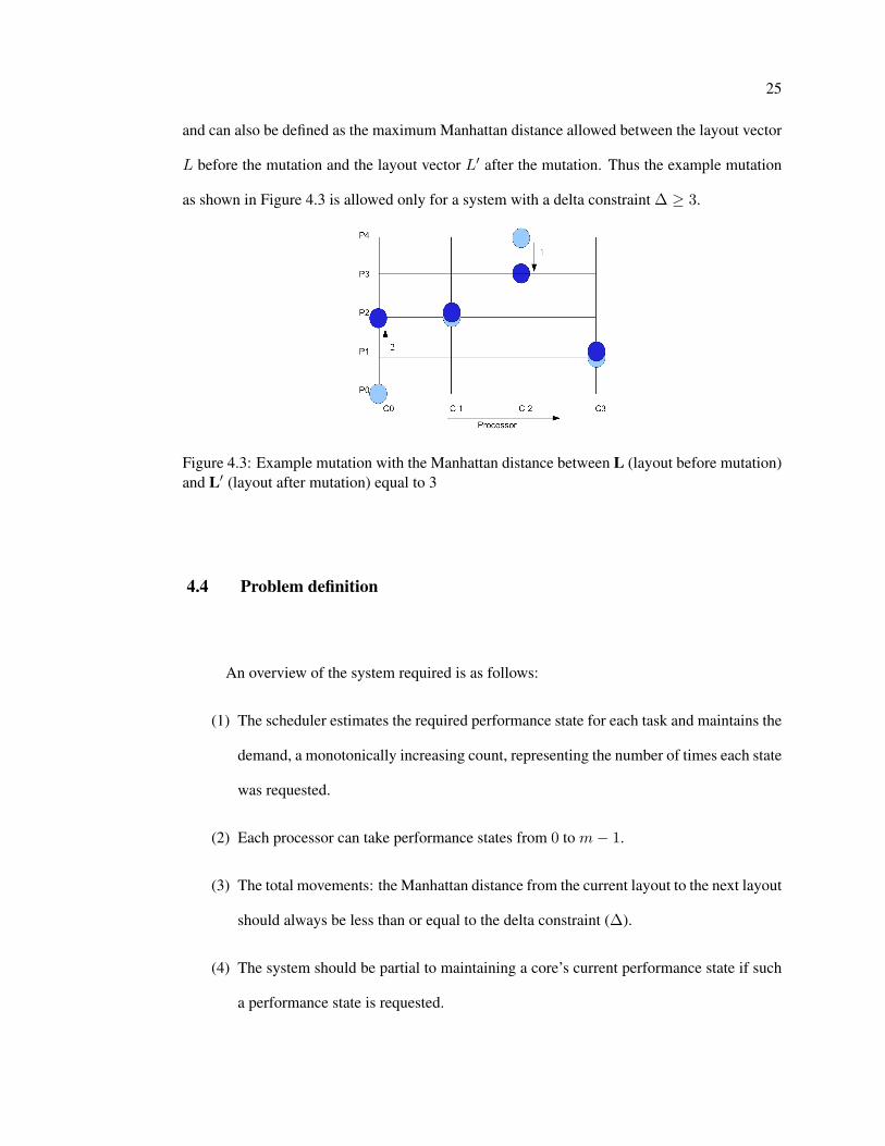
and can also be defined as the maximum Manhattan distance allowed between the layout vector
L before the mutation and the layout vector L′ after the mutation. Thus the example mutation
as shown in Figure 4.3 is allowed only for a system with a delta constraint ∆ ≥ 3.
Figure 4.3: Example mutation with the Manhattan distance between L (layout before mutation)and L′ (layout after mutation) equal to 3
4.4 Problem definition
An overview of the system required is as follows:
(1) The scheduler estimates the required performance state for each task and maintains the
demand, a monotonically increasing count, representing the number of times each state
was requested.
(2) Each processor can take performance states from 0 to m− 1.
(3) The total movements: the Manhattan distance from the current layout to the next layout
should always be less than or equal to the delta constraint (∆).
(4) The system should be partial to maintaining a core’s current performance state if such
a performance state is requested.
26
The problem can be expressed as a multiple choice knapsack problem with each variable
xi (corresponding to each processor) capable of m options thus xij
xij ∈ {0, 1}, i = 0, 1, 2, ..., n− 1; j = 0, 1, 2, ...,m− 1 (4.5)
is a 0-1 choice of selecting performance state j for processor i. As we can at most select one
performance state to a processor, the problem is restricted by
m−1∑j=0
xij = 1,∀i = 0, 1, ..., n− 1 (4.6)
which allows only one of the choices for all performance states j. The knapsack capacity is the
delta constraint (∆) thus bringing the constraint of the optimization problem to be
Subject to :n−1∑i=0
m−1∑j=0
|Li − j|xij ≤ ∆ (4.7)
where xij is the selection of the transition of processor i from performance state Li to j. Finally
the problem is to optimize the transitions in such a way as to optimally satisfy the demand
vector D by
maxn−1∑i=0
m−1∑j=0
Djxij (4.8)
Defining the problem this way, the memorization based dynamic programming method
described in [19] was implemented. Early experimental results showed that the algorithm was
inefficient for having no concept of transition direction, that is, the algorithm attempts to fill
the knapsack (performing enough transitions within the constraint of ∆) without distinguishing
between transitions which increase performance from transitions which decrease performance.
Another effect which is not accounted by the dynamic programming approach is to ig-
nore the fact that the algorithm will be repeated periodically and the current results will be
utilized as the problem during the next mutation interval. Thus the dynamic programming ap-
proach tries to perfect the selection even though the layout adaptation can always be perfected
in future mutation intervals, Implying that the required nature of adaptation is to at least gravi-
tate towards the optimal layout. This motivated the development of an iterative direction based
greedy algorithm described below.
27
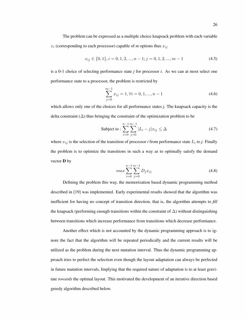
4.5 The delta constrained mutation algorithm
Figure 4.4 describes the steps involved in the proposed iterative greedy algorithm. Each
sub step is described in further sections. The initialization procedure is described in Sec-
tion 4.5.1. Based on the iteration delta constraint δ, a matrix, Manhattan matrix (S) is con-
structed and described in Section 4.5.2. The Manhattan weight vector W is described in Sec-
tion 4.5.3. The cooperative demand transformation is described in 4.5.4. The greedy winning
state w selection is described in Section 4.5.5. The selection of the processor c to transition
to the winning state w is described in Section 4.5.6. Finally, the parameter adjustments and
iteration termination conditions are described in Section 4.5.7.
Figure 4.4: Mutation algorithm
28
4.5.1 Initialization
In order to effectively provide only the needed number of processors, the mutator queries
the operating system for the total number of tasks in the ready state T . The Load of the system
Load =
T : T ≤ n
n : T > n
(4.9)
in terms of number of processors required is computed where T is the total number of tasks
in the ready state in a multicore system with n on-line cores. Using an estimated load based
on idle times of processors was found to be unfruitful as it can be non-representative of the
actual computing capacity demanded by the number of active tasks. This can be aggravated in
situations where multiple tasks could be queued on a single processor.
4.5.1.1 Processor demand
The Performance Directed Scheduler as described in Chapter 3 maintains the demand
for each state in the demand vector D. The contents of this vector cannot be directly consumed
as their values pose no direct description of the demand of individual performance states. As a
direct consequence, vector demand is computed based on the projected load of the system and
the demand vector D,
demandi =Di × Load
m−1∑j=0
Dj
(4.10)
where Di is the total number of times performance state Pi was requested by the performance
directed scheduler in the previous mutation interval while the total load of the system was
estimated to be load. The vector demand is also referred to as the core demand as each element
demandi is the total number of cores demanded by the performance directed scheduler at state
Pi in order to optimally schedule the current workload.
29
4.5.1.2 Present and required power characteristic of the system
powerP the present or current power number of the multicore system,
powerP =n−1∑i=0
Li (4.11)
where n is the total number of on-line cores and L is the current layout of the system. Thus
powerP is an integer value proportional to the total power drawn by the multicore system.
powerR, the required power number
powerR =m−1∑i=0
i× demandi (4.12)
is computed based on the processor demand demand as shown below in Equation (4.12) where,
each core is capable of m performance states and demandi being the total number of cores
demanded by performance state Pi. Thus powerR is proportional to the power drawn by the
multicore system when the cores are transitioned in such a way as to satisfy the performance
directed scheduler to optimally schedule it’s current workload.
4.5.1.3 Transition direction
Based on the parameters powerP and powerR, the transition direction, trans, a tri-state
value trans ∈ {−1, 0,+1} describing the nature of mutation required
trans =
1 : powerR > powerP
0 : powerR = powerP
−1 : powerR < powerP
(4.13)
is computed. This is done by the mutation engine to evaluate the required direction in which
DVFS configuration must be made. A transition direction of trans = +1 implies that the
scheduler requires higher performance from the multicore system, while a transition direction
of trans = −1 implies the exact opposite; an indication to conserve power by reducing the
30
performance states of the multicore processor. A transition direction equal to zero implies
stability and mutations must be avoided if possible.
4.5.1.4 Poison vector and iteration delta constraint initialization
Before starting the iterations, the poison vector X of length n
∀i ∈ N, i < n;Xi = 1 (4.14)
is initialized to all ones, where each element is a binary representation (Xi ∈ {0, 1}) of a
unique processor’s current assignment states. A value Xi = 0 indicates that processor i has
been allocated a performance state and must not be re-transitioned. Finally, the iteration delta
constraint δ is initialized to ∆ (δ = ∆).
4.5.2 The Manhattan matrix
The Manhattan matrix S with n rows (one for each core) and m columns (one for each
performance state), can be viewed as a probability matrix where each element Sij indicates the
probability that processor i can be transitioned to performance state j for a system with n cores
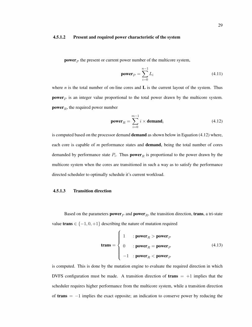
each capable of m performance states and depicted in Figure 4.5. Thus S23 describes the weight
of processor C2 transitioning to the performance state P3. The conception of this matrix was
achieved by viewing a probability density function for each processor and was soon modified
due to the lack of floating point operations in kernel space (Even though possible, the kernel
address space does not save the floating point context and makes it’s use dangerous as the kernel
is fully preempt-able).
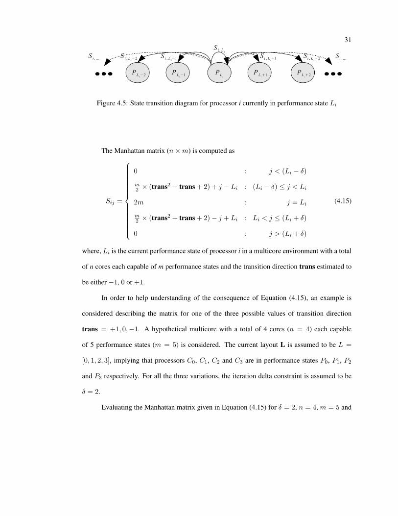
31
Figure 4.5: State transition diagram for processor i currently in performance state Li
The Manhattan matrix (n×m) is computed as
Sij =
0 : j < (Li − δ)
m2 × (trans2 − trans + 2) + j − Li : (Li − δ) ≤ j < Li
2m : j = Li
m2 × (trans2 + trans + 2)− j + Li : Li < j ≤ (Li + δ)
0 : j > (Li + δ)
(4.15)
where, Li is the current performance state of processor i in a multicore environment with a total
of n cores each capable of m performance states and the transition direction trans estimated to
be either −1, 0 or +1.
In order to help understanding of the consequence of Equation (4.15), an example is
considered describing the matrix for one of the three possible values of transition direction
trans = +1, 0,−1. A hypothetical multicore with a total of 4 cores (n = 4) each capable
of 5 performance states (m = 5) is considered. The current layout L is assumed to be L =
[0, 1, 2, 3], implying that processors C0, C1, C2 and C3 are in performance states P0, P1, P2
and P3 respectively. For all the three variations, the iteration delta constraint is assumed to be
δ = 2.
Evaluating the Manhattan matrix given in Equation (4.15) for δ = 2, n = 4, m = 5 and

32
L = [0, 1, 2, 3] and all values of trans,
Strans=+1 =
10 9 8 0 0
4 10 9 8 0
3 4 10 9 8
0 3 4 10 9
(4.16)
Strans=0 =
10 4 3 0 0
4 10 4 3 0
3 4 10 4 3
0 3 4 10 4
(4.17)
Strans=−1 =
10 4 3 0 0
9 10 4 3 0
8 9 10 4 3
0 8 9 10 4
(4.18)
is obtained. The following observations and reasoning can be made about these variations of
the Manhattan matrix:
• For each row, i, the highest weight of 2m (10), is assigned to the element Sij when
j = Li.
◦ As L0 = 0, the element S00 = 10.
◦ The highest weight is given to a transition favoring a processor to maintain its
current performance state if required.
• For each row, i, elements Sij are assigned a value of 0, when they are more that δ
elements away (|j − Li| > δ) from the current performance state.
◦ Elements S03 and S04 are assigned a value of 0.
◦ This honors the iteration delta constraint δ by assigning a weight (probability)
equal to zero to such transitions.

33
• For each row, i, and column Li < j ≤ (Li + δ), integer weights are assigned to Sij
such that they are in decreasing order starting from 2m − 1 (9) for trans = +1 or
starting from m− 1 (4) for trans = 0 and trans = −1.
◦ Weights for transitions linearly reduce as they are further from the current perfor-
mance state.
◦ Strans=+1: Elements S01, S02 are given values 9 and 8 respectively and weights
linearly reduce from 2m− 1 (9) as transition direction trans = +1 indicates that
mutations (DVFS reconfigurations) must favor transitions increasing the perfor-
mance of the multicore.
◦ Strans=0,−1: Elements S01, S02 are given values 4 and 3 respectively and reduce
from m − 1 for trans = −1, 0 as mutations must not favor transitions increas-
ing the power consumption of the multicore system for trans = −1 or avoid
transitions for trans = 0.
• For each row, i, and column (Li− δ) ≤ j < Li, integer values are assigned to Sij such
that they are in decreasing order starting from 2m − 1 (9) for trans = −1 or starting
from m− 1 (4) for trans = 0 and trans = +1.
◦ Weights for transitions linearly reduce as they are further from the current perfor-
mance state.
◦ Strans=−1: Elements S21, S20 are given values 9 and 8 respectively and weights
linearly reduce from 2m − 1 (9) as transition direction trans = −1 indicates
that mutations (DVFS reconfigurations) must favor transitions reducing the power
consumption of the multicore.
◦ Strans=0,+1: Elements S21, S20 are given values 4 and 3 respectively and reduce
from m − 1 for trans = +1, 0 as mutations must not favor transitions reducing
the performance of the multicore system for trans = +1 or avoid transitions for
34
trans = 0.
4.5.3 The Manhattan weight vector
The Manhattan weight vector W
∀j ∈ N : j < m;Wj =n−1∑i=0
Sij (4.19)
is constructed where n is the total number of cores and m is the total number of performance
states avaliable in each core. The Manhattan weight vector is achieved by summing along each
column of the Manhattan matrix and hence providing an insight into the locality of each state. A
higher value of Wi indicates a higher probability that there exists active processors in or around
performance state i, while a null value, Wi = 0 indicates that the performance state i can never
be achieved under the current delta constraint.
4.5.4 Cooperative demand distribution: The demand field
With lower values of ∆ (or with respect to the current iteration, δ), there is a possibility
that a state i, could be requested with a high core demand (demandi) but due to the current
layout and delta constraint, have a Manhattan weight Wi = 0, implying that a core in perfor-
mance state i can never be provided. Thus a method was developed in transforming the vector
demand in such a way that such null performance states cooperatively give up their demand to
the performance state closest to them which has a possibility of being selected. This procedure
is described in Algorithm 1.
The demand field F is essentially a replicate of demand, and differs under circumstances
when, for a particular performance state i, Wi = 0 and demandi > 0, then its demand is dis-
tributed to a friend f which varies based on the transition direction trans. If transition direction
trans = 1, then the demand is given to the state f closest and lesser than i with Wf > 0. If the
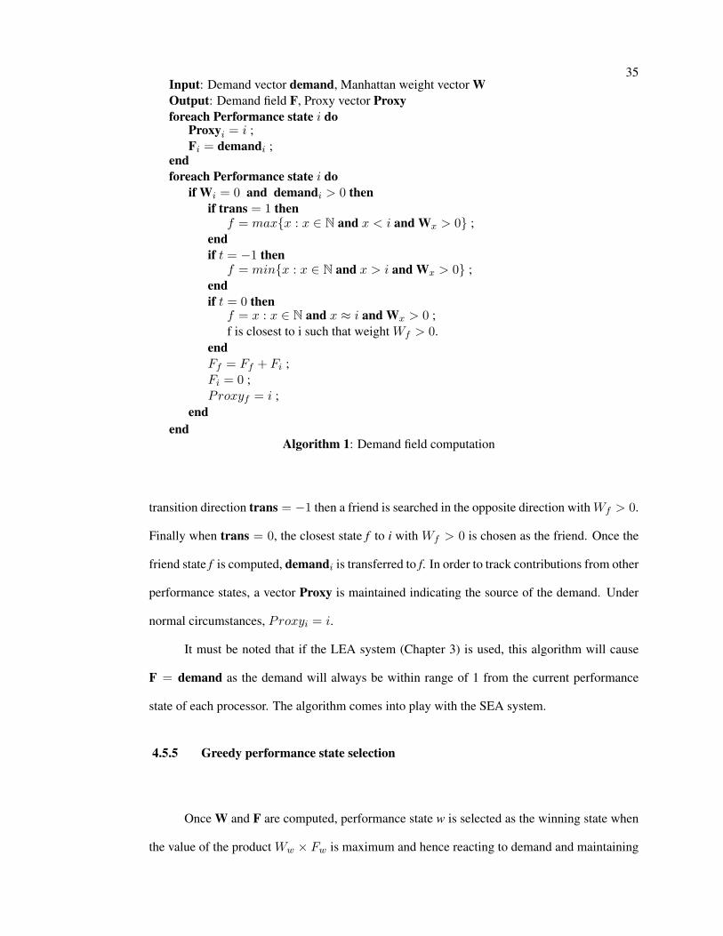
35Input: Demand vector demand, Manhattan weight vector WOutput: Demand field F, Proxy vector Proxyforeach Performance state i do
Proxyi = i ;Fi = demandi ;
endforeach Performance state i do
if Wi = 0 and demandi > 0 thenif trans = 1 then
f = max{x : x ∈ N and x < i and Wx > 0} ;endif t = −1 then
f = min{x : x ∈ N and x > i and Wx > 0} ;endif t = 0 then
f = x : x ∈ N and x ≈ i and Wx > 0 ;f is closest to i such that weight Wf > 0.
endFf = Ff + Fi ;Fi = 0 ;Proxyf = i ;
endend
Algorithm 1: Demand field computation
transition direction trans = −1 then a friend is searched in the opposite direction withWf > 0.
Finally when trans = 0, the closest state f to i with Wf > 0 is chosen as the friend. Once the
friend state f is computed, demandi is transferred to f. In order to track contributions from other
performance states, a vector Proxy is maintained indicating the source of the demand. Under
normal circumstances, Proxyi = i.
It must be noted that if the LEA system (Chapter 3) is used, this algorithm will cause
F = demand as the demand will always be within range of 1 from the current performance
state of each processor. The algorithm comes into play with the SEA system.
4.5.5 Greedy performance state selection
Once W and F are computed, performance state w is selected as the winning state when
the value of the product Ww × Fw is maximum and hence reacting to demand and maintaining
36
locality. the winning state w
w = arg maxx
Wx × Fx (4.20)
4.5.6 Greedy processor selection and transition
With the winning performance state selected, the processor to be transitioned is deter-
mined by the row c
c = arg maxx
Sxw ×Xx (4.21)
in the Manhattan matrix whose value Scw × Xc is maximum. Once the selection is made,
processor c is transitioned to performance state w by invoking the seeker cpufreq governor
described in Section 4.2. An addition, not mentioned in Figure 4.4 in order to maintain clarity,
is to abort the iteration algorithm if the value Scw = 0. This condition implies that there are no
more available processors which are capable of transitions due to the iteration delta constraint.
4.5.7 Parameter change and termination conditions
At the end of every iteration, the parameters δ, Lc and demandw are updated to represent
the transition. First as a transition was previously performed, the iteration delta constraint must
reduce
δ = δ − |Lc − w| (4.22)
by an equal order as a part of the iteration delta constraint δ is consumed by the current transi-
tion. Second, as processor c is no longer in performance state Lc, it is updated to it’s new value
w
Lc = w (4.23)
thus future iterations are aware of the current locality. Third, as a processor is assigned to
37
performance state w, the corresponding demand
demandProxyw = demandProxyw − 1 (4.24)
can be decremented. Note that, due to the distortion introduced by the cooperative demand dis-
tribution, demandProxyw is updated instead of demandw. Lastly, the poison vector’s position
for processor c
Xc = 0 (4.25)
is set to zero and hence disabling processor c in participating in a future transitions. It can be
observed from Equation (4.21) that a value of 0 for Xi will ensure that i will never be used as
the resulting value of Xi × Siw will be zero and will never be selected, achieving the desired
behavior.
This concludes a single iteration of the greedy direction based algorithm and is repeated
for Load iterations as long as the iteration delta constraint δ > 0. The upper bound on the
number of iterations is Load (Which can be at most n) and ensures early termination of the
iterative algorithm when unnecessary.
The algorithmic complexity of the entire procedure assuming n >> m, can be evaluated
to be O(n2), as the number of iterations can be at most n, and each iteration involves the eval-
uation of the Manhattan matrix which can have up to n rows. Note that the complexity of the
described procedure is the same as that of the dynamic programming approach (with memo-
rization) but is more efficient due to the consideration of transition direction. The complexity is
affordable as this is executed at a much coarser interval (mutation interval), if not, the mutation
interval can be increased to reduce the effects of the evaluation time.
Chapter 5
Experimental setup and results
A Linux kernel module as shown in Figure 5.1 was developed incorporating the ideas
discussed in chapters 3 and 4. The scheduling routines in the Linux kernel (To be specific,
schedule and switch to) were extended using kprobes [20] to add the performance directed
scheduling features. The choice to use kprobes [20] a feature essentially used for debugging
and instrumentation from the context of a kernel module pose two possible problems. One,
kprobes by themselves introduce unnecessary code paths and interrupts causing some if not
significant overhead (Less than 3%). Secondly, certain functions relating to migration are not
exported to kernel modules and hence indirect and suboptimal procedures were chosen to get the
necessary functionality. In spite of these disadvantages, having the project as a kernel module
accelerated the development process.
For a system with m total performance states and n total processors, ∆ can at most take
a value of n× (m− 1). Experiments were carried on a quad-core AMD Opteron (Barcelona),
and a patched version of the Linux 2.6.28 kernel. The logging interface as shown in Figure 5.1,
collects task specific and system wide statistics which enable in studying the behavior of both
the performance directed scheduler and the delta constrained mutator. The statistics collected by
the logging system aided in the computation of total energy consumption of each processor and
workload. In order to measure percentage slowdown, the six workloads mentioned in Chapter 2,
were run with full clock speed, recording their cumulative execution time. The power values
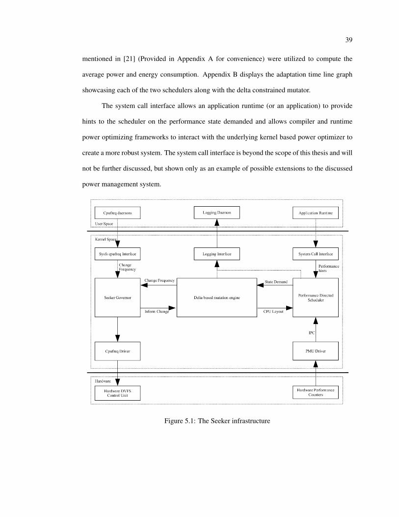
39
mentioned in [21] (Provided in Appendix A for convenience) were utilized to compute the
average power and energy consumption. Appendix B displays the adaptation time line graph
showcasing each of the two schedulers along with the delta constrained mutator.
The system call interface allows an application runtime (or an application) to provide
hints to the scheduler on the performance state demanded and allows compiler and runtime
power optimizing frameworks to interact with the underlying kernel based power optimizer to
create a more robust system. The system call interface is beyond the scope of this thesis and will
not be further discussed, but shown only as an example of possible extensions to the discussed
power management system.
Figure 5.1: The Seeker infrastructure

40
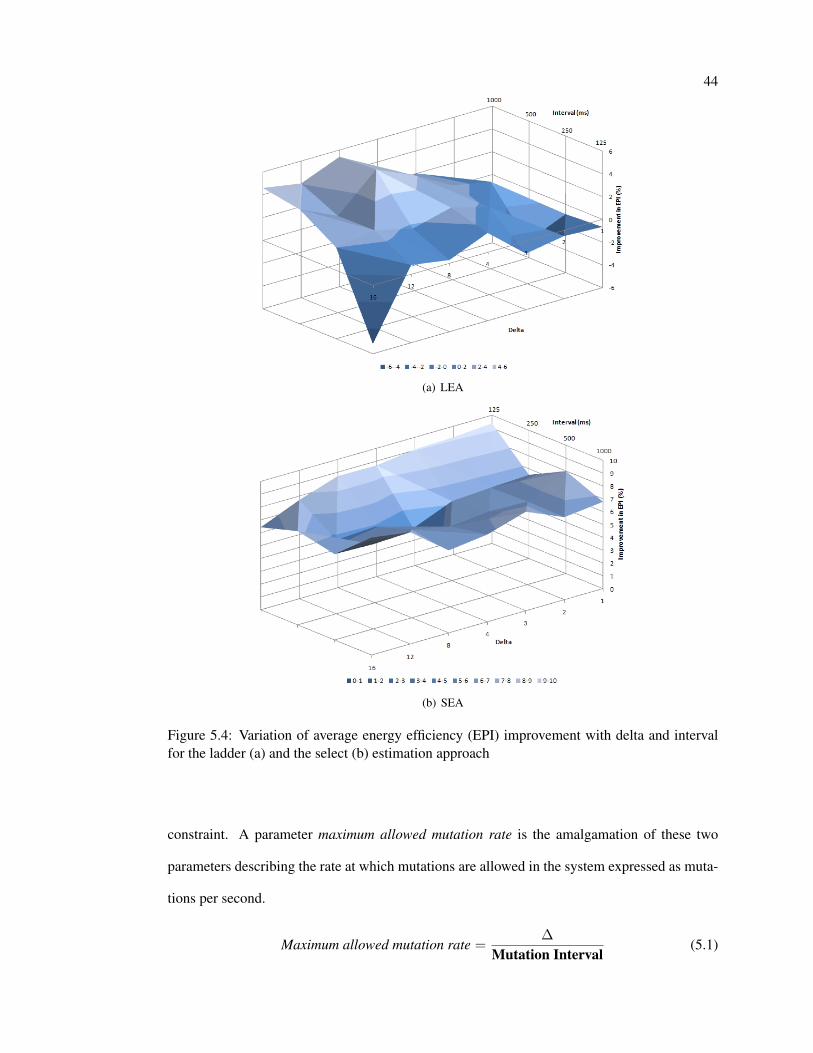
5.1 Trends along delta and interval
Two parameters namely the delta constraint (∆) and the mutation interval were intro-
duced in Chapter 4. In order to further study the system it is important to define the variation of
three important effects, namely, slowdown and power savings and energy efficiency improve-
ment as a function of these parameters. A fully factorial experiment was conducted varying
delta from 1 through 16 and the interval from 125ms through 1000ms. All the six workloads
in Table 2.2 (Chapter 2) were run for each experiment. Slowdown for each workload was com-
puted by comparing it’s execution time to that when run on a multicore system with all cores
executing with the maximum frequency. Power savings was computed by comparing the aver-
age power consumption to the highest being 115.0W per core. And finally Energy efficiency
improvement was computed by comparing the EPI of each experiment to that when all cores
are executing with the maximum possible clock speed.
Figure 5.2 shows the trends observed with respect to slowdown for the LEA and SEA
scheduling systems. An unnaturally high slowdown can be observed for small values of delta
(∆) which can be attributed to the plasticity in adaptation. The interval of mutation has little
significance towards slowdown for delta values higher than 3.The mutation interval begins to
play a vital role in differentiating the experiments based on slowdown once the delta constraint
is lowered beyond a value of 3. It can be observed that at lower values of delta, reducing
the mutation interval has an effect of decreasing the slowdown and effectively reducing the
performance lost. Comparing Figure 5.2(a) with 5.2(b) shows that lower values of delta have a
more profound negative effect on the SEA system than the LEA system. At ∆ = 1, the SEA
system exhibits at least 5% higher slowdown but both rapidly falls to the plateau close to 10%
beyond a delta constraint of 4.
The logging interface was configured to sample the executing workload’s characteris-
tic and namely the execution time and current performance state (which was used to arrive
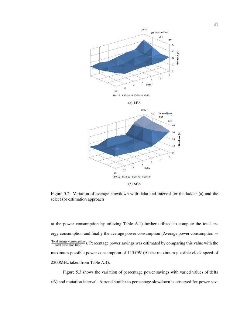
41
(a) LEA
(b) SEA
Figure 5.2: Variation of average slowdown with delta and interval for the ladder (a) and theselect (b) estimation approach
at the power consumption by utilizing Table A.1) further utilized to compute the total en-
ergy consumption and finally the average power consumption (Average power consumption =
Total energy consumptiontotal execution time ). Percentage power savings was estimated by comparing this value with the
maximum possible power consumption of 115.0W (At the maximum possible clock speed of
2200MHz taken from Table A.1).
Figure 5.3 shows the variation of percentage power savings with varied values of delta
(∆) and mutation interval. A trend similar to percentage slowdown is observed for power sav-
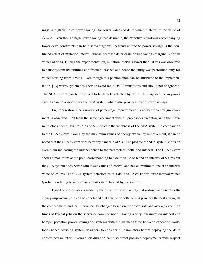
42
ings: A high value of power savings for lower values of delta which plateaus at the value of
∆ = 3. Even though high power savings are desirable, the effective slowdown accompanying
lower delta constraints can be disadvantageous. A trend unique to power savings is the con-
tinued effect of mutation interval, whose decrease deteriorate power savings marginally for all
values of delta. During the experimentation, mutation intervals lower than 100ms was observed
to cause system instabilities and frequent crashes and hence the study was performed only for
values starting from 125ms. Even though this phenomenon can be attributed to the implemen-
tation, [13] warns system designers to avoid rapid DVFS transitions and should not be ignored.
The SEA system can be observed to be largely affected by delta. A sharp decline in power
savings can be observed for the SEA system which also provides lower power savings.
Figure 5.4 shows the variation of percentage improvement in energy efficiency (improve-
ment in observed EPI) from the same experiment with all processors executing with the maxi-
mum clock speed. Figures 5.2 and 5.3 indicate the weakness of the SEA system in comparison
to the LEA system. Going by the maximum values of energy efficiency improvement, it can be
noted that the SEA system does better by a margin of 5%. The plot for the SEA system sports an
even plain indicating the independence to the parameters: delta and interval. The LEA system
shows a maximum at the point corresponding to a delta value of 8 and an interval of 500ms but
the SEA system does better with lower values of interval and has an minimum line at an interval
value of 250ms. The LEA system deteriorates at a delta value of 16 for lower interval values
(probably relating to unnecessary elasticity exhibited by the system).
Based on observations made by the trends of power savings, slowdown and energy effi-
ciency improvement, it can be concluded that a value of delta ∆ = 4 provides the best among all
the compromises and the interval can be changed based on the arrival rate and average execution
times of typical jobs on the server or compute node. Having a very low mutation interval can
hamper potential power savings for systems with a high mean time between execution work-
loads hence advising system designers to consider all parameters before deploying the delta
constrained mutator. Average job duration can also affect possible deployments with respect
43
(a) LEA
(b) SEA
Figure 5.3: Variation of average power savings with delta and interval for the ladder (a) and theselect (b) estimation approach
to mutation interval. Care must be taken to choose the mutation interval as a fraction of the
average execution times of typical jobs running on the system.
5.2 Trends along maximum allowed mutation rate
Figures 5.2, 5.3 and 5.4 shows the variation of slowdown, average power savings and
energy efficiency improvement respectively as a function of mutation interval and the delta
44
(a) LEA
(b) SEA
Figure 5.4: Variation of average energy efficiency (EPI) improvement with delta and intervalfor the ladder (a) and the select (b) estimation approach
constraint. A parameter maximum allowed mutation rate is the amalgamation of these two
parameters describing the rate at which mutations are allowed in the system expressed as muta-
tions per second.
Maximum allowed mutation rate =∆
Mutation Interval(5.1)
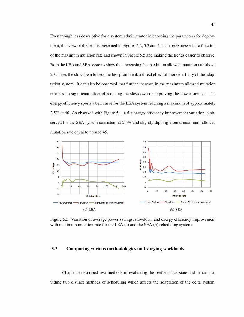
45
Even though less descriptive for a system administrator in choosing the parameters for deploy-
ment, this view of the results presented in Figures 5.2, 5.3 and 5.4 can be expressed as a function
of the maximum mutation rate and shown in Figure 5.5 and making the trends easier to observe.
Both the LEA and SEA systems show that increasing the maximum allowed mutation rate above
20 causes the slowdown to become less prominent; a direct effect of more elasticity of the adap-
tation system. It can also be observed that further increase in the maximum allowed mutation
rate has no significant effect of reducing the slowdown or improving the power savings. The
energy efficiency sports a bell curve for the LEA system reaching a maximum of approximately
2.5% at 40. As observed with Figure 5.4, a flat energy efficiency improvement variation is ob-
served for the SEA system consistent at 2.5% and slightly dipping around maximum allowed
mutation rate equal to around 45.
(a) LEA (b) SEA
Figure 5.5: Variation of average power savings, slowdown and energy efficiency improvementwith maximum mutation rate for the LEA (a) and the SEA (b) scheduling systems
5.3 Comparing various methodologies and varying workloads
Chapter 3 described two methods of evaluating the performance state and hence pro-
viding two distinct methods of scheduling which affects the adaptation of the delta system.

46
Chapter 4 introduced a common power management system, the ondemand power optimizer.
Experiments were conducted varying the mutation interval from 125ms to 1000ms for all three
systems. Section 5.1 recommends the minimum value of delta ∆ = 4 in order to minimize
the effects of slowdown due to adaptation plasticity and hence the delta mutator with a value of
∆ = 4 was utilized for the experiments proposed in this section. Utilizing the logging interface,
the execution sample performance state (and in turn the power consumption), execution time
and retired instructions were recorded to later compute the average power consumption for each
workload, the energy efficiency, measured as energy consumption per executed instruction and
slowdown. These experiments were repeated for each of the power management systems:
• Ondemand governor, mutation interval: 125ms, 250ms, 500ms, 1000ms
• The ladder performance directed scheduling system with the delta constrained mutator
with a delta value, ∆ = 4 and mutation interval: 125ms, 250ms, 500ms, 1000ms
• The select performance directed scheduling system with the delta constrained mutator
with a delta value, ∆ = 4 and mutation interval: 125ms, 250ms, 500ms, 1000ms
For each experiment, the percentage power savings, percentage slowdown and EPI (energy per
instruction) improvement was computed and tabulated. These experiments were clustered based
on workload in order to further categorize the results.
Due to the adaptive nature of the power management mechanism and the high depen-
dence on the IPC characteristic of workloads, it can be hypothesized that workloads with lower
IPC (The Low workload) should expect the maximum power savings while, workloads with
large IPC (The High workload) should expect the minimum slowdown and power savings.
Figure 5.6 shows the average values of the parameter space for each workload under
varying mutation intervals for the LEA system and the delta mutation engine. The High work-
load suffers from an insignificant value of slowdown (around 1%) but also gains no power
savings. There is a small deterioration of energy efficiency which can be perceived to be in-
significant. Meanwhile, the Low workload achieves an excess of 40% power savings with a
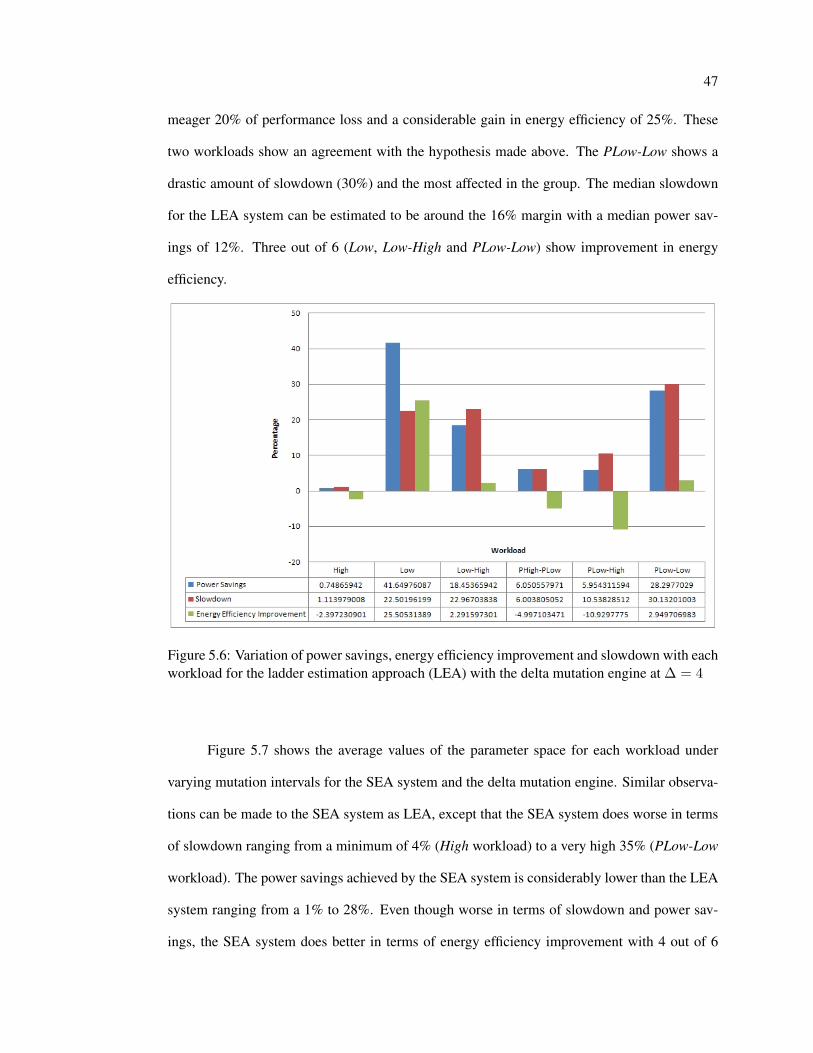
47
meager 20% of performance loss and a considerable gain in energy efficiency of 25%. These
two workloads show an agreement with the hypothesis made above. The PLow-Low shows a
drastic amount of slowdown (30%) and the most affected in the group. The median slowdown
for the LEA system can be estimated to be around the 16% margin with a median power sav-
ings of 12%. Three out of 6 (Low, Low-High and PLow-Low) show improvement in energy
efficiency.
Figure 5.6: Variation of power savings, energy efficiency improvement and slowdown with eachworkload for the ladder estimation approach (LEA) with the delta mutation engine at ∆ = 4
Figure 5.7 shows the average values of the parameter space for each workload under
varying mutation intervals for the SEA system and the delta mutation engine. Similar observa-
tions can be made to the SEA system as LEA, except that the SEA system does worse in terms
of slowdown ranging from a minimum of 4% (High workload) to a very high 35% (PLow-Low
workload). The power savings achieved by the SEA system is considerably lower than the LEA
system ranging from a 1% to 28%. Even though worse in terms of slowdown and power sav-
ings, the SEA system does better in terms of energy efficiency improvement with 4 out of 6
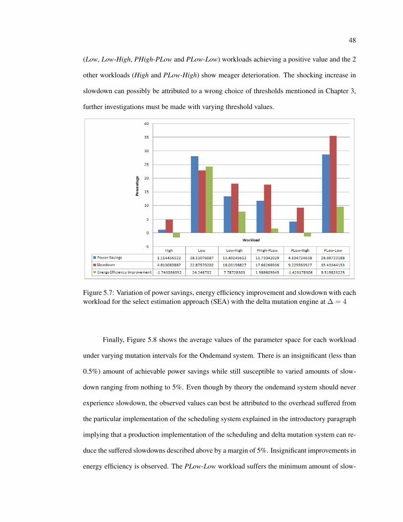
48
(Low, Low-High, PHigh-PLow and PLow-Low) workloads achieving a positive value and the 2
other workloads (High and PLow-High) show meager deterioration. The shocking increase in
slowdown can possibly be attributed to a wrong choice of thresholds mentioned in Chapter 3,
further investigations must be made with varying threshold values.
Figure 5.7: Variation of power savings, energy efficiency improvement and slowdown with eachworkload for the select estimation approach (SEA) with the delta mutation engine at ∆ = 4
Finally, Figure 5.8 shows the average values of the parameter space for each workload
under varying mutation intervals for the Ondemand system. There is an insignificant (less than
0.5%) amount of achievable power savings while still susceptible to varied amounts of slow-
down ranging from nothing to 5%. Even though by theory the ondemand system should never
experience slowdown, the observed values can best be attributed to the overhead suffered from
the particular implementation of the scheduling system explained in the introductory paragraph
implying that a production implementation of the scheduling and delta mutation system can re-
duce the suffered slowdowns described above by a margin of 5%. Insignificant improvements in
energy efficiency is observed. The PLow-Low workload suffers the minimum amount of slow-
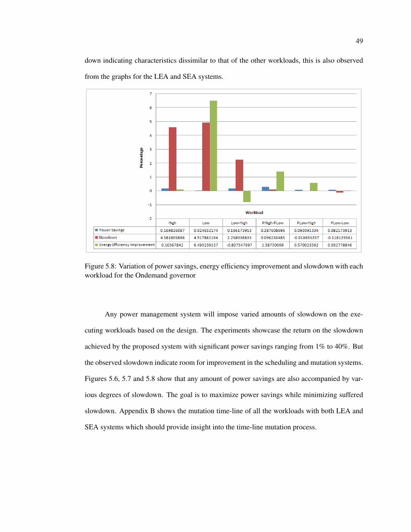
49
down indicating characteristics dissimilar to that of the other workloads, this is also observed
from the graphs for the LEA and SEA systems.
Figure 5.8: Variation of power savings, energy efficiency improvement and slowdown with eachworkload for the Ondemand governor
Any power management system will impose varied amounts of slowdown on the exe-
cuting workloads based on the design. The experiments showcase the return on the slowdown
achieved by the proposed system with significant power savings ranging from 1% to 40%. But
the observed slowdown indicate room for improvement in the scheduling and mutation systems.
Figures 5.6, 5.7 and 5.8 show that any amount of power savings are also accompanied by var-
ious degrees of slowdown. The goal is to maximize power savings while minimizing suffered
slowdown. Appendix B shows the mutation time-line of all the workloads with both LEA and
SEA systems which should provide insight into the time-line mutation process.

Chapter 6
Future work
The scheduling methodology can integrate the work presented in [22] for higher accu-
racy in predicting the performance state required by a particular task. Further analysis on the
relationship of clock speed invariance of workloads may prove valuable in improving the select
scheduling system and deriving a more optimal methodology of selecting its threshold values.
The fact that there exists a correlation between IPC and speedup achievable with increased
clock speed, can be further utilized to produce a more robust system. The first steps would be
to provide strong support within the Linux kernel for asymmetric multicore processors which
will enable further study into the aspect of performance directed scheduling.
A system call interface was integrated into the existing system which can be utilized
to develop compiler or runtime frameworks, which would potentially have more information
about program characteristics in developing a hybrid system to provide higher power savings
with lower performance loss.
Chapter 7
Summary and Conclusion
This thesis presented an approach of scheduling tasks on multicore processors with re-
spect to performance requirements and performing a constrained system wide dynamic voltage
and frequency transitions in reaction to the demands of the performance characteristic of the
executing workloads. A novel methodology was presented in controlling the magnitude of
these transitions to improve stability and longevity of the multicore system. The methodology
was shown to possess characteristics to minimize slowdown of workloads while improving the
power savings achieved.
Workloads were shown to possess characteristics to possibly make it immune to clock
speed improvements thus enhancing the motivation of a performance determined power man-
agement system to conserve power during system active state. Experiments with various static
layouts were conducted to characterize and showcase the performance directed scheduler. It
was demonstrated that a statically assigned performance state layout of a system can prove
to drastically deteriorate performance of the system in an environment with non-deterministic
workload sets. Two scheduling systems, the ladder and select, were developed to schedule tasks
based on their performance characteristic.
A system was developed to allow a performance directed scheduler to direct an asyn-
chronously run power optimizer to manage the performance states of each core in an otherwise
homogeneous multicore environment. The problem was shown to be NP-Hard and an efficient
52
algorithm was developed in solving the Multiple-choice knapsack problem as a direction based
iterative greedy algorithm.
Experiments were conducted to measure slowdown and power savings along the sys-
tem’s entire parameter space to determine the most favorable constraint on the magnitude of the
allowed DVFS transitions. This was utilized to compare the power management system with a
popular load based power optimizer, the ondemand governor. The combination of the perfor-
mance directed scheduler and the delta constrained mutator was shown to achieve higher power
efficiency and better power savings with marginal slowdown.
Bibliography
[1] W. Kim, M. S. Gupta, G.-Y. Wei, and D. Brooks, “System level analysis of fast, per-coredvfs using on-chip switching regulators,” in 2008 IEEE 14th International Symposiumon High Performance Computer Architecture. Piscaatway, NJ, USA: IEEE, 2008, pp.123–134.
[2] K. M. P. R. M. K. M. J. Irwin, “Phase-aware adaptive hardware selection for power-efficient scientific computations,” in International Symposium on Computer Architecture/Proceedings of the 2007 international symposium on Low power electronics and design.Portland, OR, USA: ACM, 2007, pp. 403–406.
[3] M. Kondo, H. Sasaki, and H. Nakamura, “Improving fairness, throughput and energy-efficiency on a chip multiprocessor through dvfs,” vol. 35, no. 1. New York, NY, USA:ACM, 2007, pp. 31–38.
[4] Q. Wu, M. Martonosi, D. W. Clark, V. J. Reddi, D. Connors, Y. Wu, J. Lee, andD. Brooks, “A dynamic compilation framework for controlling microprocessor energy andperformance,” in MICRO 38: Proceedings of the 38th annual IEEE/ACM InternationalSymposium on Microarchitecture. Washington, DC, USA: IEEE Computer Society,2005, pp. 271–282.
[5] H. Sasaki, Y. Ikeda, M. Kondo, and H. Nakamura, “An intra-task dvfs technique basedon statistical analysis of hardware events,” in Conference On Computing Frontiers/Proceedings of the 4th international conference on Computing frontiers. Ischia, Italy:ACM, 2007, pp. 123–130.
[6] A. Rangasamy, R. Nagpal, and Y. Srikant, “Compiler-directed frequency and voltage scal-ing for a multiple clock domain microarchitecture,” in CF ’08: Proceedings of the 5thconference on Computing frontiers. New York, NY, USA: ACM, 2008, pp. 209–218.
[7] B. Rountree, D. K. Lownenthal, B. R. de Supinski, M. Schulz, V. W. Freeh, and T. Bletsch,“Adagio: making dvs practical for complex hpc applications,” in ICS ’09: Proceedings ofthe 23rd international conference on Supercomputing. New York, NY, USA: ACM, 2009,pp. 460–469.
[8] B. Rountree, D. K. Lowenthal, S. Funk, V. W. Freeh, B. R. de Supinski, and M. Schulz,“Bounding energy consumption in large-scale mpi programs,” in SC ’07: Proceedings ofthe 2007 ACM/IEEE conference on Supercomputing. New York, NY, USA: ACM, 2007,pp. 1–9.
54
[9] K. Meng, R. Joseph, R. P. Dick, and L. Shang, “Multi-optimization power managementfor chip multiprocessors,” in Proceedings of the 17th international conference on Parallelarchitectures and compilation techniques. Toronto, Ontario, Canada: ACM, 2008, pp.177–186.
[10] C. Isci, G. Contreras, and M. Martonosi, “Live, runtime phase monitoring and predictionon real systems with application to dynamic power management,” in In: Proceedings ofthe 39th International Symposium on Microarchitecture (MICRO-39). Los Alamitos,CA, USA: IEEE Computer Soc, 2006, p. 12pp.
[11] Y.-H. Lu, L. Benini, and G. D. Micheli, “Operating-system directed power reduction,” inConference On Computing Frontiers/ Proceedings of the 4th international conference onComputing frontiers. Rapallo, Italy: ACM, 2000, pp. 37–42.
[12] C. Boneti, R. Gioiosa, F. J. Cazorla, and M. Valero, “A dynamic scheduler for balanc-ing hpc applications,” in SC ’08: Proceedings of the 2008 ACM/IEEE conference onSupercomputing. Piscataway, NJ, USA: IEEE Press, 2008, pp. 1–12.
[13] N. Soundararajan, N. Vijaykrishnan, and A. Sivasubramaniam, “Impact of dynamicvoltage and frequency scaling on the architectural vulnerability of gals architectures,”in ISLPED ’08: Proceeding of the thirteenth international symposium on Low powerelectronics and design. New York, NY, USA: ACM, 2008, pp. 351–356.
[14] Standard Performance Evaluation Corporation, “The SPEC CPU 2006 benchmark suite,”2006. [Online]. Available: http://www.spec.org
[15] T. Li, D. Baumberger, D. A. Koufaty, and S. Hahn, “Efficient operating system schedulingfor performance-asymmetric multi-core architectures,” in SC ’07: Proceedings of the 2007ACM/IEEE conference on Supercomputing. New York, NY, USA: ACM, 2007, pp. 1–11.
[16] D. P. Gulati, C. Kim, S. Sethumadhavan, S. W. Keckler, and D. Burger, “Multitaskingworkload scheduling on flexible-core chip multiprocessors,” in Proceedings of the 17thinternational conference on Parallel architectures and compilation techniques. Toronto,Ontario, Canada: ACM, 2008, pp. 187–196.
[17] R. Nathuji and K. Schwan, “Virtualpower: coordinated power management in virtualizedenterprise systems,” in SOSP ’07: Proceedings of twenty-first ACM SIGOPS symposiumon Operating systems principles. New York, NY, USA: ACM, 2007, pp. 265–278.
[18] V. Pallipadi and A. Starikovskiy, “The on-demand governor,” in 2006 LinuxSymposium, 2006. [Online]. Available: http://ftp.funet.fi/pub/Linux/kernel/people/lenb/acpi/doc/OLS2006-ondemand-paper.pdf
[19] J. C. Bean, “Multiple choice knapsack functions,” in Proceedings of the 2007 InternationalSymposium on Low-Power Electronics and Design (ISLPED’07), Department of Indus-trial operations and Engineering, University of michigan, Ann Arbor, Michigan 48109,1987.
[20] R. Krishnakumar, “Kernel korner: kprobes-a kernel debugger,” Linux J., vol. 2005, no.133, p. 11, 2005.
55
[21] AMD, AMD Family 10h Server and Workstation Processor Power and Thermal DataSheet, June 2009. [Online]. Available: http://support.amd.com/us/Processor TechDocs/43374.pdf
[22] M. Curtis-Maury, A. Shah, F. Blagojevic, D. S. Nikolopoulos, B. R. de Supinski, andM. Schulz, “Prediction models for multi-dimensional power-performance optimization onmany cores,” in Proceedings of the 17th international conference on Parallel architecturesand compilation techniques. Toronto, Ontario, Canada: ACM, 2008, pp. 250–259.
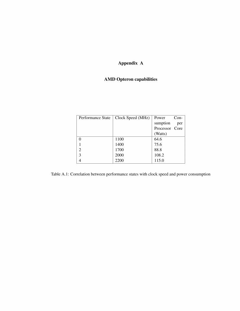
Appendix A
AMD Opteron capabilities
Performance State Clock Speed (MHz) Power Con-sumption perProcessor Core(Watts)
0 1100 64.61 1400 75.62 1700 88.83 2000 108.24 2200 115.0
Table A.1: Correlation between performance states with clock speed and power consumption
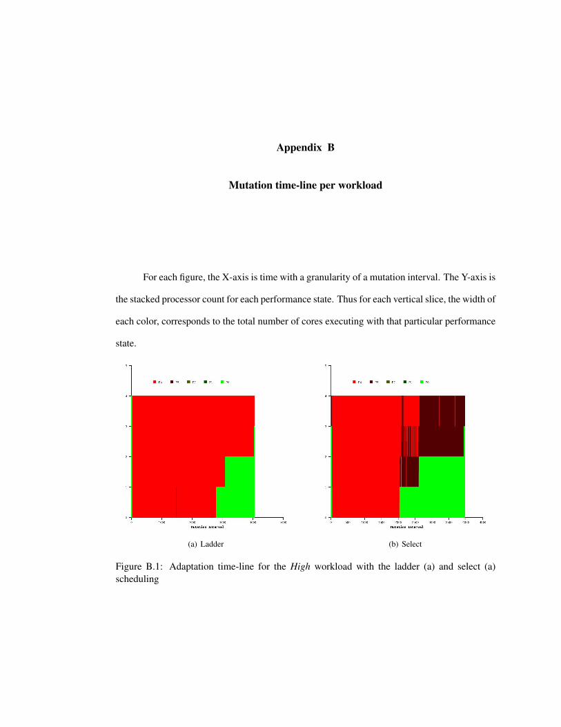
Appendix B
Mutation time-line per workload
For each figure, the X-axis is time with a granularity of a mutation interval. The Y-axis is
the stacked processor count for each performance state. Thus for each vertical slice, the width of
each color, corresponds to the total number of cores executing with that particular performance
state.
(a) Ladder (b) Select
Figure B.1: Adaptation time-line for the High workload with the ladder (a) and select (a)scheduling
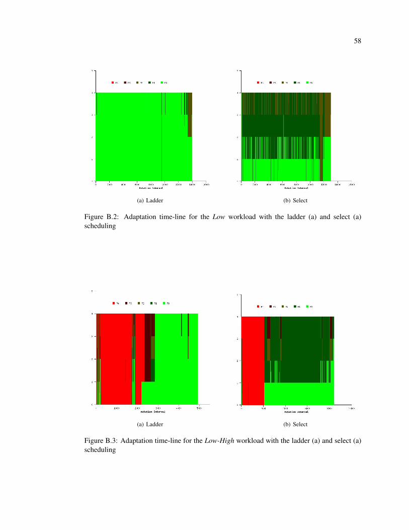
58
(a) Ladder (b) Select
Figure B.2: Adaptation time-line for the Low workload with the ladder (a) and select (a)scheduling
(a) Ladder (b) Select
Figure B.3: Adaptation time-line for the Low-High workload with the ladder (a) and select (a)scheduling
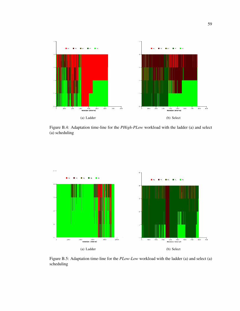
59
(a) Ladder (b) Select
Figure B.4: Adaptation time-line for the PHigh-PLow workload with the ladder (a) and select(a) scheduling
(a) Ladder (b) Select
Figure B.5: Adaptation time-line for the PLow-Low workload with the ladder (a) and select (a)scheduling
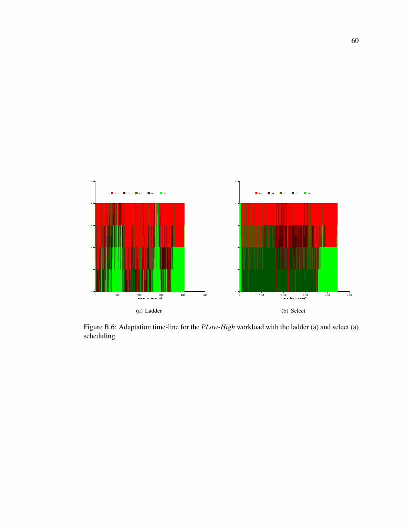
60
(a) Ladder (b) Select
Figure B.6: Adaptation time-line for the PLow-High workload with the ladder (a) and select (a)scheduling

Appendix C
Source code
All the source code has been uploaded in a public git repository and available at:
git://github.com/amithash/seeker-scheduler.git.
Note that in order to checkout the source code, you will need to have the git source
control management utilities installed.