Encoded Invariance in Convolutional NeuralNetworks

Nathaniel SauderUniversity of Chicago

nsauder@uchicago.edu

Abstract

Deep neural networks have proven remarkably effective on tasks where euclideandistance in the raw input space lacks semantic meaning and thus where an inter-mediate representation must be constructed before the usual suite of classifiers canbe used effectively. Traditionally, these representations were painstakingly hand-crafted in order to capture a sufficiently strong signal while reducing dimension.However, deep learning methods attempt to learn this representation over manyexamples. In this paper, we review and propose methods of encoding invariancein the learnt representations whereby the requisite dimension reduction can beachieved while nonetheless preserving the signal.

1 Neural Networks

1.1 Biological Inspiration

Neural networks were inspired by central nervous systems. However their machine learning imple-mentations are simple to describe: repeated compositions of linear maps with non-linear activationfunctions. The biological analogs are dendrites sending neurotransmitters into a neuron which thenpasses the signal along to its neighbors if a threshold is met. Convolutional neural networks fix someweights to be equal. In particular, they encode the 2d translational covariance, i.e filters applied inthe top right patch will also be applied in the bottom left. Invariance and covariance are essentialto the success of convolutional neural networks. Indeed, the name requires a group structure overwhich to convolve. In computer vision, this group has traditionally been the set of 2d translationswhile in time series or speech modelling it has been the 1d time axis. In this paper, we proposemethods for how convolutional neural networks might encode further, more complex invariance.

1.2 Applications

Convolutional Neural Networks are widely applied. Indeed, they are currently dominant on a varietyof benchmarks in computer vision. Krizhevsky 2012 Imagenet ConvNet trained on 2 GPUs standsout as demonstrating the power of these methods. [1] However, ConvEnts have also performed wellon seemingly unrelated tasks like classifying the quantum physical quantities of proposed molecules.[2]

1.3 Layers in Convolutional Neural Nets

ConvEnts are composed of several different types of layers. Convolutional layers compute responsemaps derived from convolving a 3d filter across the feature maps in the previous layer. Activationfunctions are then computed for each point and are analogous to thresholding in actual neurons.Sigmoids and hyperbolic tangents are popular choices however ReLUs, max(0, x), are increasinglyused due to their sparse output and lack of saturation. These altered response maps then undergo

1

spatial subsampling or pooling, biologically inspired by Hubel and Wiesels work in the 1960s onmodels of human vision, where local responses – for instance, 7x7 windows – are pooled into asingle value for input into the ensuing layer. After several layers of stacked convolution, activation,pooling blocks, the outputs are fed into a series of fully connected layers before softmax generatesthe class probabilities. Much experimentation has taken place regarding the optimal procedure foreach of these components however we will briefly mention two more methods that were critical toKrizhevsky et al.s success in 2012: Local Response Normalization and Dropout. LRN layer involvenormalizing weights at a specific point (x, y) over n feature maps. LRNs create competition betweenneurons for large activations. These make particular sense in the last convolutional layer as thesefeatures tend to be as high-level as houses or sheep – mutually exclusive categories. Finally, Dropoutprevents cohabitation of features by randomly dropping half of the neurons in the fully connectedlayers. Given sufficient sparsity, Dropout approaches model averaging over exponentially manymodels.[3]

Figure 1: Basic architecture of ConvNets – missing many of the layers just discussed

2 Pooling

2.1 Introduction

Pooling is the primary source of dimension reduction and of local translation invariance in a Con-vNet. Accordingly, pooling mechanisms are judged by how much they can reduce the dimensionwhile preserving the signal. Invariance of the image class under local group actions are thus es-sential to understanding how these dueling objectives can be balanced. Theoretical results indicatethat all forms of `p pooling preserve the signal provided the feature maps are sufficiently redundant.[4] However, in practise, different pooling mechanisms offer stark changes in performance. Accord-ingly, we consider and propose several pooling regimes, catalog their results on benchmark data-setswhile providing some mathematical and computer vision to support their effects.

2.2 Ave vs Max

There are two main approaches to pooling: averaging the responses and taking their maximum.These are complementary in that they belong on opposite ends of the `p spectrum:

`1 ⇐⇒ avg`∞ ⇐⇒ max

Examining their differences will motivate the recently implemented pooling regimes as well thosewe are introducing ourselves. Boureau et al. have written the main paper on the subject whichadvocates using max pooling when representations are sparse. Intuitively, this seems reasonable asthe presence of a house in a part of an image should not be diluted by its absence in other regions.[5] Similarly, the firing of a vertical edge detector in a part of the image should not be diluted byits absence in a local region. The outputs of average and max pooling networks in [6] confirm theintuition that average pooling dilutes the signal excessively. picture

2.3 Heterogeneous Pooling

An alternative to debating whether max or average is universally preferable is to include both in thenetwork. In particular, under this scheme some feature maps are pooled by max, others by average.Indeed, for spatially distinct complex features (keypoints, maybe edge-like structure), max is likelypreferable; whereas for feature maps that are less spatially localized, e.g., color or broad texture, av-erage may be better. In our experiments, performance was essentially identical to max pooling while

2

Figure 2: Effects of max andaverage on signal quality. [6] Figure 3: Visualizations of 2nd layer of Imagenet network. [7]

convergence was marginally quicker. Heterogeneous pooling can be easily extended to an arbitrarynumber of different pooling regimes. Finally, another alternative is feeding each set of responsesto a suite of pooling regimes and thereby increasing the signal preservation while hampering thedimensionality reduction. In sum, while performance was not improved by adopting heterogenouspooling mechanisms within the same network, we believe that heterogenous applications of poolingmay prove fruitful as there is substantial variety both within filter banks – color vs edge – as well asbetween layers – color vs house detector.

2.4 `p Pooling

Another natural extension of the max/avg debate is to observe that avg and max lie on opposite endsof the `p spectrum and question whether intermediate values may be optimal. In 2012, Sermanet etal. tested this hypothesis on the Street View House Numbers dataset where the task is identifying thestreet number from house signs. [8] They also chose pooling regions with significant overlap andperformed `p pooling with a Gaussian envelope instead of pure `p pooling. Not only is the optimalnorm not average or max, the advantage offered by choosing the optimal norm, `4 is significant:3% improvement. While these results would suggest that grid search on the optimal norm for agiven problem might yield a choice other than average or max, more recent experiments suggestthat if p <∞ then the model averaging approximation of dropout is weakened sufficiently to erodeperformance.

2.5 Stochastic and Entropy Pooling

Whether max or avg pooling is chosen, the resulting ConvNets overfit significantly. [6] Borrowingfrom the main idea of dropout: stochastically removing neurons in order to train each independently,Zeiler and Fergus propose a similar probabilistic regime for pooling. In particular, the probabilityof propagating response wij for the region P is wij∑

P wijwhere the sum is taken over all units in

the pooling region. As this generates too much noise when testing, they choose E(P ) as outputunder those conditions. The effect is a large reduction in overfitting resulting in substantiallybetter performance on the suite of benchmark small datasets: CIFAR-10, CIFAR-100, SVHN, andMNIST. To explain their results, Zeiler and Fergus argue that stochastic pooling enables modelaveraging in the convolutional layers. Furthermore, they claim that stochastic pooling ensures adegree of deformational invariance. Accordingly, it would be instructive to test Szegedys adversarialexamples, [9], on a ConvNet with stochastic pooling.

3

As just discussed, a stochastic pooling ConvNet take the expectation of the response when testing.We observe that this amounts to `22

`1pooling. They report that training with expectation pooling

encounters the same troubles with overfitting. However, perhaps the superiority of max poolingsuggests that pooling with probabilities assigned proportionally to an `p norm would yield stronger

results. Instead of obeying the `2n+1

`nrestriction, we tried entropy pooling: `2∞

`1or max2

avg . Intuitively,given a clear peak in response the output of entropy pooling will be proportional to the squaredheight of the peak; whereas for uniform responses, the output will be the average. 1 Essentially,this amounts to TF-IDF pooling – weighing down more common responses. Empirically however itdoes not offer an improvement.

2.6 Maxout

Building off the immense success Dropout training methods have had, [3], Goodfellow et al. soughtto specifically design an activation function to improve the model averaging approximation. [10]Maxout units take the maximum of responses over a specific pooling region across multiple fea-ture maps. However, maxout is an activation function as ReLUs are not applied to the responsesbefore being fed into the maxout unit. (Indeed, doing so causes a 0.2% reduction in performanceon MNIST) As a consequence, the response can be negative. An entire maxout unit can be seen asan universal approximator as any continuous function can be approximated by the maximum of aset of convex and concave functions. Thus, in a sense, the ideal activation function is being learnt.A potential example of a maxout unit involves maxing over two vertical edge detectors: one withrightward gradient and the other leftward. Taking the max of the two produces a positive responseif there is an edge regardless of direction of color change. Goodfellow et al. claim that sparsity andnon-saturation allows for closer approximations to model averaging. Furthermore, the increasedsparsity of the gradient allows for the global minimum to be more easily approximated.

Given competing evidence for different pooling schemes, it is natural to ask whether the optimalnorm can be learnt. Accordingly, Gulcehre et al. implement an `p unit that computes the `p normover the responses in a spatial region across several feature maps. [11] However, the value of p in`p is learnt by backprop. The authors justify this use by arguing that the curved boundaries offeredby the ellipses of `p units allow for more realistic approximation of the true activation function.Interestingly, for MNIST their optimal norm value is 3.4 – similar to the optimal choice, 4, of [8].Indeed they also find that different units prefer similar norm values: the standard deviation is 0.38.[summary argument]

2.7 Global Pooling

Both maxout and learned norm pooling increase the complexity of the convolutional layers by in-troducing highly non-linear activation and pooling functions. Network in Network goes further byconvolving with a 3 layer neural network rather than linear filters. [12] As this offers a great in-crease in complexity in the convolutional layers, the authors remove all fully connected layers byglobal average pooling across the last feature maps and feeding the resulting vector into the soft-max layer. Furthermore, they require that the number of feature maps is equal to the number ofclasses thereby learning one feature map per class. Their explanation also relies on the language ofuniversal approximation. After all, a 3 layer MLP is a universal approximator and thus can theoret-ically approach any filter. However, if we accept Mallats interpretation of the convolutional layersas rotations of the input space – to be followed by pooling contractions – then the non-linearity ofthe filter is immaterial. Indeed, under this interpretation the non-linearities in ReLUs and poolingoperators are sufficient to achieve the non-linear twists in the decision boundary. Nonetheless, theresults of NIN are excellent and furthermore they improve with the difficulty of the task. Successfulperformance on the significantly more challenging Imagenet data-set would certainly validate thisapproach further.

Perhaps of greater relevance to architecture choice in regular ConvNets is the global average poolingundertaken in the last convolutional layer. Indeed, Network in Network [12] show that global averagepooling is also an effective regularization technique for traditional ConvNets. While it does notoutperform dropout, it does improve upon the usual arrangement of fully connected layers. That

1While maxavg

might seem initially more appealing, it is discontinuous at zero.

4

Figure 4: Left, convolution by linear filter. Right, convolution by 3 layer neural network [12]

a crude measure such as global averaging offers an improvement demonstrates the severity of theoverfitting in the fully connected layers. Finally, it seems plausible that global max pooling wouldoutperform global average pooling as max pooling would capture the simple existence of an objectin the space whereas average pooling would dilute this signal – given the features learnt in the lastconvolutional layer, max pooling seems the obvious choice. Another benefit to these scheme isits invariance to aspect ratios of the input. While in classification tasks the input images have aconsistent, usually dyadic shape, in detection the bounding boxes can be irregular.The current Stateof the Art on detection [13] addresses this problem by resizing the image to fit the desired size of theConvNets thereby incurring a significant loss of information. Global pooling thus offers a simplealternative.

2.8 Summary

In sum, a heterogeneous approach to pooling seems preferable as the difference in the filters meritdifferent approaches. Whereas the final layer benefits substantially from local response normaliza-tion and more generally from competition among its neurons, the earlier filters seem more comple-mentary than adversarial. Indeed, whereas the earlier layers perhaps should be viewed primarilyfrom a mathematical perspective: as first order Taylor approximations of the local ”surface – colorfilters as measurements of height and edge filters as a measure of local gradients, the later layersseem more approachable by computer vision heuristics. Accordingly, we believe that varying pool-ing mechanisms both between layers and within layers will result in improvements in classificationas well as detection, given more experimentation.

3 Invariance

3.1 Rigid Motion Invariance

Having explored a mechanism by which the ConvNets forcibly encodes a symmetry invariance –local translation – a natural question arises: how much invariance does a ConvNets learn withoutenforcing symmetry through architecture decisions. In particular, how different are the representa-tions of two images which differ only by an affine action? By a small deformation? Goodfellow etal. reveal that they are very consistent across actions by rigid motion while highly unstable underadversarial deformation. Measuring Invariances in Deep Networks employs convolutional sparseencoders in order to measure invariance with respect to SO2, SO3 and T by observing whetherneurons continue to fire while image is acted upon by group elements. Goodfellow et al. find thatinvariance is highly dependent on the depth of the architecture especially 3D rotations.

3.2 Invariance under Deformations

Invariance under deformation has been less studied however a recent paper presented some surpris-ing results. [9] Given an image and a small choice of epsilon, they were able to find an adversarialexample with the ball β(image, ε). In fact, for most images Szegedy et al. are able to find one that isvisually indistinguishable and yet classified as an ostrich. Furthermore, these adversarial examplespersist across different architectures, i.e. the found examples are robust. Finally, a spectral analy-sis of each of the layers in a SOA Imagenet network [1] revealed that the convolutional layers hadlarge lipschitz coefficients while also finding that the lipschitz bound was sufficiently high to allow

5

for highly expansive mappings. Accordingly, this result indicates that ConvEnts are not robust todeformation. Nonetheless, the Imagenet network continues to classify at 51% level on images thatare distorted by random gaussian noise. Therefore, it is clear that while networks are not invariantto distortion, not much performance is lost on distortion errors.

Figure 5: Left, original image classified correctly. Center, difference between left and right images.Right, classified as an ostrich. [9]

Thus, we find that our ConvNets are stable to action by rigid motions yet highly unstable undersmall deformations. Accordingly, we would like to find a representation that has a small lipschitzcoefficient: it maps nearby points in image space to nearby points in the representation space. Adeep learning evangelist may argue that we should simply learn these invariances and not constrainthe architecture. The following work addresses some of these concerns.

3.3 Wavelet Network Algorithm

A couple of years ago, Mallat proposed cascading wavelets filters as a means of representing nat-ural images or textures. The objective is to construct a representation that is not only invariant torigid motions as ConvNets appear to be, but also to deformations. Accordingly, Mallat proposeswavelet networks which essentially are ConvNets where the learnt linear filters are replaced by fixedwavelets. Critically, given a compact lie group, G, Mallat proves in [14] that a wavelet network canbe constructed that is invariant toG as well as stable under deformations. In particular, the algorithmcalls for choosing k multiscale wavelet filters and convolving them with the image space over thedesired group of actions – for example, 2d translations and rotations. Applying the modulus opera-tion to each response yields k non-negative response fields. Now, convolve each feature map withthe same suite of wavelets and reapply the modulus operator. Doing so to the desire depth, d, yieldskd feature maps. At the end, subsample using Gaussian `1 pooling and feed the resulting (scatter-ing) coefficients into a linear classifier. In sum, wavelet networks provide theoretical guarantees ofinvariance under deformation at the cost of not learning task specific filters.

6

While the previous section describes the general flavor of the procedure, some facts are worthquickly mentioning. First, clearly for computational reasons a full wavelet basis cannot be used.Secondly, as repeated modulus along a given path dilute the signal, responses that result from pathswith three or more modulus operations are discarded as well as those where the second wavelethas a higher frequency than the first. Pruning the possible paths in this way yields a complexity ofn ∗ log(n) instead of n2 for a three layer wavelet network. Thirdly, after each layer the `1 averagesof the responses are added to the representation vector. Some convolutional neural networks alsooutput each layer into the representation, i.e. multistage architectures [8].

Figure 6: scattering coefficients for digit 3. Eight rotations of wavelet are chosen hence eight scales.Each slice is divided into eighth depending on orientation of the second wavelet. Scale informationin radial direction. [15]

3.4 Pooling in Wavelet Networks

Unlike Boureau et al. suggest and other ConvNets implement, Mallat and Bruna find that averagepooling outperforms max pooling. Indeed, it does so by 8% when using complex wavelets whileaverage and max perform equally well when employing real wavelets. They justify this result byderiving the `1 norm as the only functional, M , that satisfies the following conditions:

1) commutes with deformations: M ◦ Λτ = Λτ ◦M2) unitary: ‖Mx‖ = ‖x‖

3) lipshitz condition: ‖Mx−My‖ ≤ ‖x− y‖

Finally, as the wavelet representations can be inverted with the wavelet transform little informationis lost – (some is lost as the full frequency is not employed). It would be interesting to see whetherthe distinction between average and max in regular ConvNets evaporates if multistage architecturesare employed.

3.5 MNIST experiment

Mallat and Bruna first apply these networks to MNIST. The convolution is only over the translationgroup while the wavelets are scaled and rotated. Note this differs from ConvEnts where the invari-ance group are again 2d translations however the filters are not required to be scaled and rotatedversions of a mother fitler. They derive near SOA results on the canonical dataset. The scatteringcoefficients are fed into PCA regression as well as an SVM. In an additional test that illustratesthe strength of the invariance in these networks, the authors rotate randomly rotate the digits inthe MNIST Dataset – removing 9s – and rerun their experiments and compare against a retrainedConvNet. The wavelet wetwork dramatically outperforms the ConvNet.[15]

3.6 Texture and Image Classification Experiments

Sifre and Mallat extended this work by attempting to build invariance to the entire affine group ratherthan simply the group of translations. One method of doing so might involve cascading a layerencoding horizontal invariance with one encoding vertical invariance with one encoding rotationalinvariance etc... In other words, suppose our desired invariance group is G and G = G1 oG2. Nowlet the first layer be invariant to G1 and covariant to G2 and the second be invariant to G2. Wethen arrive at a representation that is invariant to actions by G. However, this approach can subtlyrun astray. For example, the figure below shows that unless horizontal and vertical invariances areestablished simultaneously two different images can be mapped to the same representation. Thus,they attempt to compute the rotation and relational invariants simultaneously for the first layer whileseparating them for the second. However, as scaling obeys a power law, it can be linearized bythe logarithm and thus separated from the other invariances. Finally, as small deformations are

7

linearized by cascading wavelets networks, [14] they are eliminated in the PCA regression on thescattering coefficients.

Figure 7: Loss of information if convolutions are separately computed. [15][15]

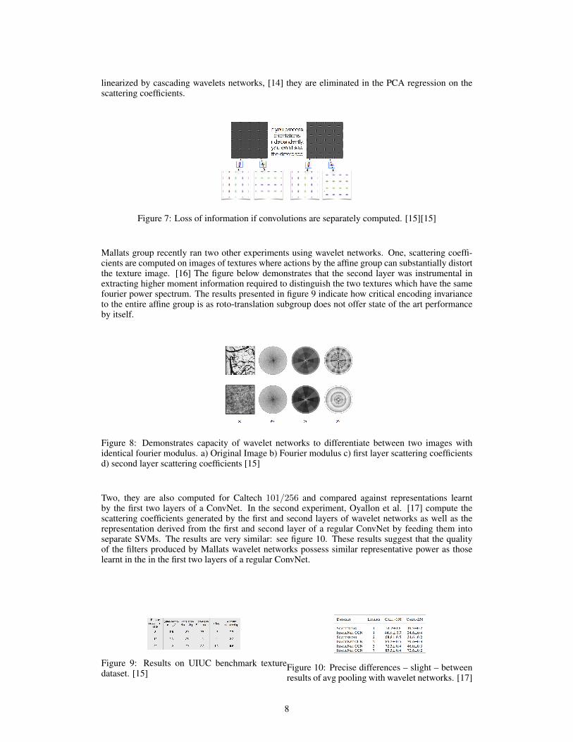
Mallats group recently ran two other experiments using wavelet networks. One, scattering coeffi-cients are computed on images of textures where actions by the affine group can substantially distortthe texture image. [16] The figure below demonstrates that the second layer was instrumental inextracting higher moment information required to distinguish the two textures which have the samefourier power spectrum. The results presented in figure 9 indicate how critical encoding invarianceto the entire affine group is as roto-translation subgroup does not offer state of the art performanceby itself.

Figure 8: Demonstrates capacity of wavelet networks to differentiate between two images withidentical fourier modulus. a) Original Image b) Fourier modulus c) first layer scattering coefficientsd) second layer scattering coefficients [15]

Two, they are also computed for Caltech 101/256 and compared against representations learntby the first two layers of a ConvNet. In the second experiment, Oyallon et al. [17] compute thescattering coefficients generated by the first and second layers of wavelet networks as well as therepresentation derived from the first and second layer of a regular ConvNet by feeding them intoseparate SVMs. The results are very similar: see figure 10. These results suggest that the qualityof the filters produced by Mallats wavelet networks possess similar representative power as thoselearnt in the in the first two layers of a regular ConvNet.

Figure 9: Results on UIUC benchmark texturedataset. [15]

Figure 10: Precise differences – slight – betweenresults of avg pooling with wavelet networks. [17]

8

4 Future Work

4.1 Small Illuminating Tweaks

In sum, there are three main methods of introducing invariance into a Conv Net: convolving overa given group and accumulating the results, altering the pooling function to include more generallocal invariance, and finally data augmentation – presenting the network with rotated images andaveraging the final probabilities. We propose some quick empirical tests to develop better intuitionfor ConvNet representations:

• repeat Girshick experiments with global max pooling; determine whether there is a rela-tionship between degree of rescaling and error rate

• varied regularization constants for fully connected and convolutional layers. Most agree,that fully connected layers are responsible for overfitting. Does independently regularizingthese layers reduce overfitting?

• visualize maxout filters in lower levels to determine how color and edge filters are beingcombined.

• regularize the lipschitz constant in the convolutional layers in order to prevent expansivebehavior in convolutional layers.

• run same adversarial paradigm to determine whether it is always possible to find rotationsor translations that result in ostrich classification

4.2 Larger Scale source of improvements

While the previous experiments offer an opportunity to develop a deeper empirical understandingof ConvNets, we believe that more fundamental improvements can be found in the following twoways:

1. Transferring the bulk of the parameter set from the fully connected layers into convolutionallayers. There are many methods are doing so: global max pooling (previously discussed),maxout was able to learn productively to significantly greater depth – 7 layers, network innetworks convolution by neural networks, and multistage architectures are some examples.It seems that Sermanets 2014 Imagenet network will illustrate the power of this approach.

2. Encoding symmetry in convolutional neural networks more explicitly. Enforcing rotation-ally symmetric and scaled filters, enforcing invariances at different layers according to thedesired locality, or factoring higher dimensional convolutions into multiplications of lowerdimensional ones. For example, while at Google, Joakim Anden factored the 3d convolu-tions in an imagenet network, i.e. apply 2d filters and then pass a 1d convolution over theiroutputs to arrive a factore 3d convolution, resulting in substantially faster convergence.

4.3 Conclusion

The successful move from fully connected feed-forward neural nets to convolutional neural nets wasan insight of symmetry: local translation invariance, global translation covariance. Given that naturalimages and especially domain-specific images (houses, eyeballs, etc...) obey far more symmetries,developing a globalized framework to encode domain and hierarchical invariance would be usefulboth theoretically and practically– currently, invariance is usually provided by data augmentation ala Sander Deliemans Kaggle Galaxy Zoo solution. A step in this direction was a recent paper [18]where ConvNets were applied to generalized graphs rather just grid graphs. A final step would belearning the invariances directly from the data. While this direction proffers fanciful hopes suchas learning physics rules directly from data, in the short term we believe that increased attentionto encoding invariance may offer faster convergence, fewer examples required, and perhaps betterresults as greater depth becomes possible with reduction in parameters.

4.4 Acknowledgments

I would first like to thank Prof. Shakhnarovich for his wonderful mentorship this summer. He wasexceptionally kind in welcoming the REU students into his group. I am particularly grateful for the

9

extended time he spent with me ensuring a clean start to this project. Secondly, I would like ProfBabai and Prof Kurtz for organizing this wonderful REU as well as for preparing some wonderfulfood for the potluck.

References

[1] Alex Krizhevsky, Ilya Sutskever, and Geoffrey E. Hinton. Imagenet classification with deepconvolutional neural networks. In Peter L. Bartlett, Fernando C. N. Pereira, Christopher J. C.Burges, Lon Bottou, and Kilian Q. Weinberger, editors, NIPS, pages 1106–1114, 2012.

[2] G. Montavon, M. Rupp, V. Gobre, A. Vazquez-Mayagoitia, K. Hansen, A. Tkatchenko, K.-R.Muller, and O. Anatole von Lilienfeld. Machine learning of molecular electronic properties inchemical compound space. New Journal of Physics, 15(9):095003, September 2013.

[3] Geoffrey E. Hinton, Nitish Srivastava, Alex Krizhevsky, Ilya Sutskever, and Ruslan Salakhut-dinov. Improving neural networks by preventing co-adaptation of feature detectors. CoRR,abs/1207.0580, 2012.

[4] J. Bruna, A. Szlam, and Y. LeCun. Signal Recovery from Pooling Representations. ArXive-prints, November 2013.

[5] Y-Lan Boureau, Jean Ponce, and Yann Lecun. A theoretical analysis of feature pooling invisual recognition. In 27TH INTERNATIONAL CONFERENCE ON MACHINE LEARNING,HAIFA, ISRAEL, 2010.

[6] M. D. Zeiler and R. Fergus. Stochastic Pooling for Regularization of Deep ConvolutionalNeural Networks. ArXiv e-prints, January 2013.

[7] Matthew D. Zeiler and Rob Fergus. Visualizing and understanding convolutional networks.CoRR, abs/1311.2901, 2013.

[8] P. Sermanet, S. Chintala, and Y. LeCun. Convolutional Neural Networks Applied to HouseNumbers Digit Classification. ArXiv e-prints, April 2012.

[9] Christian Szegedy, Wojciech Zaremba, Ilya Sutskever, Joan Bruna, Dumitru Erhan, Ian J.Goodfellow, and Rob Fergus. Intriguing properties of neural networks. CoRR, abs/1312.6199,2013.

[10] I. J. Goodfellow, D. Warde-Farley, M. Mirza, A. Courville, and Y. Bengio. Maxout Networks.ArXiv e-prints, February 2013.

[11] C. Gulcehre, K. Cho, R. Pascanu, and Y. Bengio. Learned-Norm Pooling for Deep Feedforwardand Recurrent Neural Networks. ArXiv e-prints, November 2013.

[12] M. Lin, Q. Chen, and S. Yan. Network In Network. ArXiv e-prints, December 2013.[13] Ross B. Girshick, Jeff Donahue, Trevor Darrell, and Jitendra Malik. Rich feature hierarchies

for accurate object detection and semantic segmentation. CoRR, abs/1311.2524, 2013.[14] S. Mallat. Group Invariant Scattering. ArXiv e-prints, January 2011.[15] Joan Bruna and Stephane Mallat. Invariant scattering convolution networks. CoRR,

abs/1203.1513, 2012.[16] Laurent Sifre and Stephane Mallat. Rotation, scaling and deformation invariant scattering for

texture discrimination. In 2013 IEEE Conference on Computer Vision and Pattern Recognition,Portland, OR, USA, June 23-28, 2013, pages 1233–1240, 2013.

[17] Edouard Oyallon, Stephane Mallat, and Laurent Sifre. Generic deep networks with waveletscattering. CoRR, abs/1312.5940, 2013.

[18] J. Bruna, W. Zaremba, A. Szlam, and Y. LeCun. Spectral Networks and Locally ConnectedNetworks on Graphs. ArXiv e-prints, December 2013.

10