Encyclopaedia of Mathematical SciencesVolume 11

Algebra I

Consulting Editors:A.I. Kostrikin I.R. Shafarevich

Igor R. Shafarevich

Basic Notionsof Algebra

With 45 Figures

4L| Springer

Author

Igor R. ShafarevichSteklov Mathematical Institute

Russian Academy of ScienceGubkina ul. 8

117966 Moscow, Russia

Translator

Miles ReidMathematics InstituteUniversity of WarwickCoventry CV4 7AL, UK

Founding editor of the Encyclopaedia of Mathematical Sciences:R. V. Gamkrelidze

Title of the Russian edition:Itogi nauki i tekhniki, Sovremennye problemy matematiki,

Fundamental'nye napravleniya, Vol. 11, Algebra 1Publisher VINITI, Moscow 1986

Originally published as Algebra I by A. I. Kostrikin and I. R. Shafarevich (Eds.),Volume 11 of the Encyclopaedia of Mathematical Sciences.

Mathematics Subject Classification (1980): 12-XX, 20-XX

ISSN 0938-0396ISBN-10 3-540-25177-4 Springer Berlin Heidelberg New York

ISBN-13 978-3-540-25177-4 Springer Berlin Heidelberg New York

This work is subject to copyright. All rights are reserved, whether the whole or part of the material is concerned,specifically the rights of translation, reprinting, reuse of illustrations, recitation, broadcasting, reproduction on

microfilm or in any other way, and storage in databanks. Duplication of this publication or parts thereof ispermitted only under the provisions of the German Copyright Law of September 9,1965, in its current version, andpermission for use must always be obtained from Springer. Violations are liable for prosecution under the German

Copyright Law.

Springer is a part of Springer Science+Business Media GmbHspringeronline.com

©Springer-Verlag Berlin Heidelberg 2005Printed in Germany

The use of general descriptive names, registered names, trademarks, etc. in this publication does not imply, even inthe absence of a specific statement, that such names are exempt from the relevant pro-

tective laws and regulations and therefore free for general use.

Typesetting: Asco Trade Typesetting Ltd., Hong KongProduction: LE-TgX Jelonek, Schmidt & Vockler GbR, Leipzig

Cover Design: E. Kirchner, Heidelberg, GermanyPrinted on acid-free paper 46/3142 YL 543210

Basic Notions of Algebra

LR. Shafarevich

Translated from the Russianby M. Reid

Contents

Preface 4§ 1. What is Algebra? 6

The idea of coordinatisation. Examples: dictionary of quantum mechanics andcoordinatisation of finite models of incidence axioms and parallelism.

§2. Fields 11Field axioms, isomorphisms. Field of rational functions in independent variables;function field of a plane algebraic curve. Field of Laurent series and formal Laurentseries.

§ 3. Commutative Rings 17Ring axioms; zerodivisors and integral domains. Field of fractions. Polynomial rings.Ring of polynomial functions on a plane algebraic curve. Ring of power series andformal power series. Boolean rings. Direct sums of rings. Ring of continuous functions.Factorisation; unique factorisation domains, examples of UFDs.

§ 4. Homomorphisms and Ideals 24Homomorphisms, ideals, quotient rings. The homomorphisms theorem. The restric-tion homomorphism in rings of functions. Principal ideal domains; relations withUFDs. Product of ideals. Characteristic of a field. Extension in which a given poly-nomial has a root. Algebraically closed fields. Finite fields. Representing elementsof a general ring as functions on maximal and prime ideals. Integers as functions.Ultraproducts and nonstandard analysis. Commuting differential operators.

§ 5. Modules 33Direct sums and free modules. Tensor products. Tensor, symmetric and exterior powersof a module, the dual module. Equivalent ideals and isomorphism of modules. Modulesof differential forms and vector fields. Families of vector spaces and modules.

§6. Algebraic Aspects of Dimension 41Rank of a module. Modules of finite type. Modules of finite type over a principal idealdomain. Noetherian modules and rings. Noetherian rings and rings of finite type. Thecase of graded rings. Transcendence degree of an extension. Finite extensions.

2 Contents

§ 7. The Algebraic View of Infinitesimal Notions 50Functions modulo second order infinitesimals and the tangent space of a manifold.Singular points. Vector fields and first order differential operators. Higher orderinfinitesimals. Jets and differential operators. Completions of rings, p-adic numbers.Normed fields. Valuations of the fields of rational numbers and rational functions.The p-adic number fields in number theory.

§ 8. Noncommutative Rings 61Basic definitions. Algebras over rings. Ring of endomorphisms of a module. Groupalgebra. Quaternions and division algebras. Twistor fibration. Endomorphisms ofn-dimensional vector space over a division algebra. Tensor algebra and the non-commuting polynomial ring. Exterior algebra; superalgebras; Clifford algebra. Simplerings and algebras. Left and right ideals of the endomorphism ring of a vector spaceover a division algebra.

§ 9. Modules over Noncommutative Rings 74Modules and representations. Representations of algebras in matrix form. Simplemodules, composition series, the Jordan-Holder theorem. Length of a ring or module.Endomorphisms of a module. Schur's lemma

§ 10. Semisimple Modules and Rings 79Semisimplicity. A group algebra is semisimple. Modules over a semisimple ring. Semi-simple rings of finite length; Wedderburn's theorem. Simple rings of finite length andthe fundamental theorem of projective geometry. Factors and continuous geometries.Semisimple algebras of finite rank over an algebraically closed field. Applications torepresentations of finite groups.

§11. Division Algebras of Finite Rank 90Division algebras of finite rank over R or over finite fields. Tsen's theorem andquasi-algebraically closed fields. Central division algebras of finite rank over the p-adicand rational fields.

§ 12. The Notion of a Group 96Transformation groups, symmetries, automorphisms. Symmetries of dynamical sys-tems and conservation laws. Symmetries of physical laws. Groups, the regular action.Subgroups, normal subgroups, quotient groups. Order of an element. The ideal classgroup. Group of extensions of a module. Brauer group. Direct product of two groups.

§ 13. Examples of Groups: Finite Groups 108Symmetric and alternating groups. Symmetry groups of regular polygons and regularpolyhedrons. Symmetry groups of lattices. Crystallographic classes. Finite groupsgenerated by reflections.

§ 14. Examples of Groups: Infinite Discrete Groups 124Discrete transformation groups. Crystallographic groups. Discrete groups of motionof the Lobachevsky plane. The modular group. Free groups. Specifying a group bygenerators and relations. Logical problems. The fundamental group. Group of a knot.Braid group.

§ 15. Examples of Groups: Lie Groups and Algebraic Groups 140Lie groups. Toruses. Their role in Liouville's theorem.

A. Compact Lie Groups 143The classical compact groups and some of the relations between them.

B. Complex Analytic Lie Groups 147The classical complex Lie groups. Some other Lie groups. The Lorentz group.

C. Algebraic Groups 150Algebraic groups, the adele group. Tamagawa number.

Contents 3

§ 16. General Results of Group Theory 151Direct products. The Wedderburn-Remak-Shmidt theorem. Composition series, theJordan-Holder theorem. Simple groups, solvable groups. Simple compact Lie groups.Simple complex Lie groups. Simple finite groups, classification.

§ 17. Group Representations 160A. Representations of Finite Groups 163Representations. Orthogonality relations.

B. Representations of Compact Lie Groups 167Representations of compact groups. Integrating over a group. Helmholtz-Lie theory.Characters of compact Abelian groups and Fourier series. Weyl and Ricci tensors in 4-dimensional Riemannian geometry. Representations of SU(2) and SO(3). Zeeman effect.

C. Representations of the Classical Complex Lie Groups 174Representations of noncompact Lie groups. Complete irreducibility of representationsof finite-dimensional classical complex Lie groups.

§ 18. Some Applications of Groups 177A. Galois Theory 177Galois theory. Solving equations by radicals.

B. The Galois Theory of Linear Differential Equations (Picard-Vessiot Theory) 181C. Classification of Unramified Covers 182Classification of unramified covers and the fundamental groupD. Invariant Theory 183The first fundamental theorem of invariant theory

E. Group Representations and the Classification of ElementaryParticles 185

§ 19. Lie Algebras and Nonassociative Algebra 188A. Lie Algebras 188Poisson brackets as an example of a Lie algebra. Lie rings and Lie algebras.

B. Lie Theory 192Lie algebra of a Lie group.

C. Applications of Lie Algebras 197Lie groups and rigid body motion.

D. Other Nonassociative Algebras 199The Cayley numbers. Almost complex structure on 6-dimensional submanifolds of8-space. Nonassociative real division algebras.

§20. Categories 202Diagrams and categories. Universal mapping problems. Functors. Functors arising intopology: loop spaces, suspension. Group objects in categories. Homotopy groups.

§ 21. Homological Algebra 213A. Topological Origins of the Notions of Homological Algebra . . . 213Complexes and their homology. Homology and cohomology of polyhedrons. Fixedpoint theorem. Differential forms and de Rham cohomology; de Rham's theorem.Long exact cohomology sequence.

B. Cohomology of Modules and Groups 219Cohomology of modules. Group cohomology. Topological meaning of the coho-mology of discrete groups.

C. Sheaf Cohomology 225Sheaves; sheaf cohomology. Finiteness theorems. Riemann-Roch theorem.

4 Preface

§22. K-theory 230A. Topological X-theory 230Vector bundles and the functor Vec(X). Periodicity and the functors KJX). Kt(X) andthe infinite-dimensional linear group. The symbol of an elliptic differential operator.The index theorem.

B. Algebraic K-theory 234The group of classes of projective modules. Ko, Kl and Kn of a ring. K2 of a field andits relations with the Brauer group. K-theory and arithmetic.

Comments on the Literature 239References 244Index of Names 249Subject Index 251

Preface

This book aims to present a general survey of algebra, of its basic notions andmain branches. Now what language should we choose for this? In reply to thequestion 'What does mathematics study?', it is hardly acceptable to answer'structures' or 'sets with specified relations'; for among the myriad conceivablestructures or sets with specified relations, only a very small discrete subset is ofreal interest to mathematicians, and the whole point of the question is tounderstand the special value of this infinitesimal fraction dotted among theamorphous masses. In the same way, the meaning of a mathematical notion isby no means confined to its formal definition; in fact, it may be rather betterexpressed by a (generally fairly small) sample of the basic examples, which servethe mathematician as the motivation and the substantive definition, and at thesame time as the real meaning of the notion.

Perhaps the same kind of difficulty arises if we attempt to characterise in termsof general properties any phenomenon which has any degree of individuality.For example, it doesn't make sense to give a definition of the Germans or theFrench; one can only describe their history or their way of life. In the same way,it's not possible to give a definition of an individual human being; one can onlyeither give his 'passport data', or attempt to describe his appearance and charac-ter, and relate a number of typical events from his biography. This is the pathwe attempt to follow in this book, applied to algebra. Thus the book accom-modates the axiomatic and logical development of the subject together with moredescriptive material: a careful treatment of the key examples and of points ofcontact between algebra and other branches of mathematics and the naturalsciences. The choice of material here is of course strongly influenced by theauthor's personal opinions and tastes.

Preface 5

As readers, I have in mind students of mathematics in the first years of anundergraduate course, or theoretical physicists or mathematicians from outsidealgebra wanting to get an impression of the spirit of algebra and its place inmathematics. Those parts of the book devoted to the systematic treatment ofnotions and results of algebra make very limited demands on the reader: wepresuppose only that the reader knows calculus, analytic geometry and linearalgebra in the form taught in many high schools and colleges. The extent of theprerequisites required in our treatment of examples is harder to state; an ac-quaintance with projective space, topological spaces, differentiable and complexanalytic manifolds and the basic theory of functions of a complex variable isdesirable, but the reader should bear in mind that difficulties arising in thetreatment of some specific example are likely to be purely local in nature, andnot to affect the understanding of the rest of the book.

This book makes no pretence to teach algebra: it is merely an attempt to talkabout it. I have attempted to compensate at least to some extent for this by givinga detailed bibliography; in the comments preceding this, the reader can findreferences to books from which he can study the questions raised in this book,and also some other areas of algebra which lack of space has not allowed us totreat.

A preliminary version of this book has been read by F.A. Bogomolov, R.V.Gamkrelidze, S.P. Demushkin, A.I. Kostrikin, Yu.I. Manin, V.V. Nikulin, A.N.Parshin, M.K. Polyvanov, V.L. Popov, A.B. Roiter and A.N. Tyurin; I amgrateful to them for their comments and suggestions which have been incor-porated in the book.

I am extremely grateful to N.I. Shafarevich for her enormous help with themanuscript and for many valuable comments.

Moscow, 1984 I.R. Shafarevich

I have taken the opportunity in the English translation to correct a numberof errors and inaccuracies which remained undetected in the original; I am verygrateful to E.B. Vinberg, A.M. Volkhonskii and D. Zagier for pointing these out.I am especially grateful to the translator M. Reid for innumerable improvementsof the text.

Moscow, 1987 I.R. Shafarevich

6 §1. What is Algebra?

§1. What is Algebra?

What is algebra? Is it a branch of mathematics, a method or a frame of mind?Such questions do not of course admit either short or unambiguous answers.One can attempt a description of the place occupied by algebra in mathematicsby drawing attention to the process for which Hermann Weyl coined the un-pronounceable word 'coordinatisation' (see [H. Weyl 109 (1939), Chap. I, §4]).An individual might find his way about the world relying exclusively on his senseorgans, sight, feeling, on his experience of manipulating objects in the worldoutside and on the intuition resulting from this. However, there is anotherpossible approach: by means of measurements, subjective impressions can betransformed into objective marks, into numbers, which are then capable of beingpreserved indefinitely, of being communicated to other individuals who have notexperienced the same impressions, and most importantly, which can be operatedon to provide new information concerning the objects of the measurement.

The oldest example is the idea of counting (coordinatisation) and calculation(operation), which allow us to draw conclusions on the number of objects withouthandling them all at once. Attempts to 'measure' or to 'express as a number' avariety of objects gave rise to fractions and negative numbers in addition to thewhole numbers. The attempt to express the diagonal of a square of side 1 as anumber led to a famous crisis of the mathematics of early antiquity and to theconstruction of irrational numbers.

Measurement determines the points of a line by real numbers, and much morewidely, expresses many physical quantities as numbers. To Galileo is due themost extreme statement in his time of the idea of coordinatisation: 'Measureeverything that is measurable, and make measurable everything that is not yetso'. The success of this idea, starting from the time of Galileo, was brilliant. Thecreation of analytic geometry allowed us to represent points of the plane by pairsof numbers, and points of space by triples, and by means of operations withnumbers, led to the discovery of ever new geometric facts. However, the successof analytic geometry is mainly based on the fact that it reduces to numbers notonly points, but also curves, surfaces and so on. For example, a curve in the planeis given by an equation F(x, y) = 0; in the case of a line, F is a linear polynomial,and is determined by its 3 coefficients: the coefficients of x and y and the constantterm. In the case of a conic section we have a curve of degree 2, determined byits 6 coefficients. If F is a polynomial of degree n then it is easy to see that it hasj(n + l)(n + 2) coefficients; the corresponding curve is determined by thesecoefficients in the same way that a point is given by its coordinates.

In order to express as numbers the roots of an equation, the complex numberswere introduced, and this takes a step into a completely new branch of mathe-matics, which includes elliptic functions and Riemann surfaces.

For a long time it might have seemed that the path indicated by Galileoconsisted of measuring 'everything' in terms of a known and undisputed collec-

§1. What is Algebra? 7

tion of numbers, and that the problem consists just of creating more and moresubtle methods of measurements, such as Cartesian coordinates or new physicalinstruments. Admittedly, from time to time the numbers considered as known(or simply called numbers) turned out to be inadequate: this led to a 'crisis', whichhad to be resolved by extending the notion of number, creating a new form ofnumbers, which themselves soon came to be considered as the unique possibility.In any case, as a rule, at any given moment the notion of number was consideredto be completely clear, and the development moved only in the direction ofextending it:

'1,2, many' => natural numbers => integers=> rationals => reals => complex numbers.

But matrixes, for example, form a completely independent world of 'number-like objects', which cannot be included in this chain. Simultaneously with them,quaternions were discovered, and then other 'hypercomplex systems' (now calledalgebras). Infinitesimal transformations led to differential operators, for whichthe natural operation turns out to be something completely new, the Poissonbracket. Finite fields turned up in algebra, and p-adic numbers in number theory.Gradually, it became clear that the attempt to find a unified all-embracingconcept of number is absolutely hopeless. In this situation the principle declaredby Galileo could be accused of intolerance; for the requirement to 'make mea-surable everything which is not yet so' clearly discriminates against anythingwhich stubbornly refuses to be measurable, excluding it from the sphere ofinterest of science, and possibly even of reason (and thus becomes a secondaryquality or secunda causa in the terminology of Galileo). Even if, more modestly,the polemic term 'everything' is restricted to objects of physics and mathematics,more and more of these turned up which could not be 'measured' in terms of'ordinary numbers'.

The principle of coordinatisation can nevertheless be preserved, provided weadmit that the set of 'number-like objects' by means of which coordinatisationis achieved can be just as diverse as the world of physical and mathematicalobjects they coordinatise. The objects which serve as 'coordinates' should satisfyonly certain conditions of a very general character.

They must be individually distinguishable. For example, whereas all points ofa line have identical properties (the line is homogeneous), and a point can onlybe fixed by putting a finger on it, numbers are all individual: 3, 7/2, y/l, n and soon. (The same principle is applied when newborn puppies, indistinguishable tothe owner, have different coloured ribbons tied round their necks to distinguishthem.)

They should be sufficiently abstract to reflect properties common to a widecircle of phenomenons.

Certain fundamental aspects of the situations under study should be reflectedin operations that can be carried out on the objects being coordinatised: addition,multiplication, comparison of magnitudes, differentiation, forming Poissonbrackets and so on.

8 §1. What is Algebra?

We can now formulate the point we are making in more detail, as follows:

Thesis. Anything which is the object of mathematical study (curves and surfaces,maps, symmetries, crystals, quantum mechanical quantities and so on) can be'coordinatised' or 'measured'. However, for such a coordinatisation the 'ordinary'numbers are by no means adequate.

Conversely, when we meet a new type of object, we are forced to construct (orto discover) new types of 'quantities' to coordinatise them. The construction andthe study of the quantities arising in this way is what characterises the place ofalgebra in mathematics (of course, very approximately).

From this point of view, the development of any branch of algebra consists oftwo stages. The first of these is the birth of the new type of algebraic objects outof some problem of coordinatisation. The second is their subsequent career, thatis, the systematic development of the theory of this class of objects; this issometimes closely related, and sometimes almost completely unrelated to thearea in connection with which the objects arose. In what follows we will try notto lose sight of these two stages. But since algebra courses are often exclusivelyconcerned with the second stage, we will maintain the balance by paying a littlemore attention to the first.

We conclude this section with two examples of coordinatisation which aresomewhat less standard than those considered up to now.

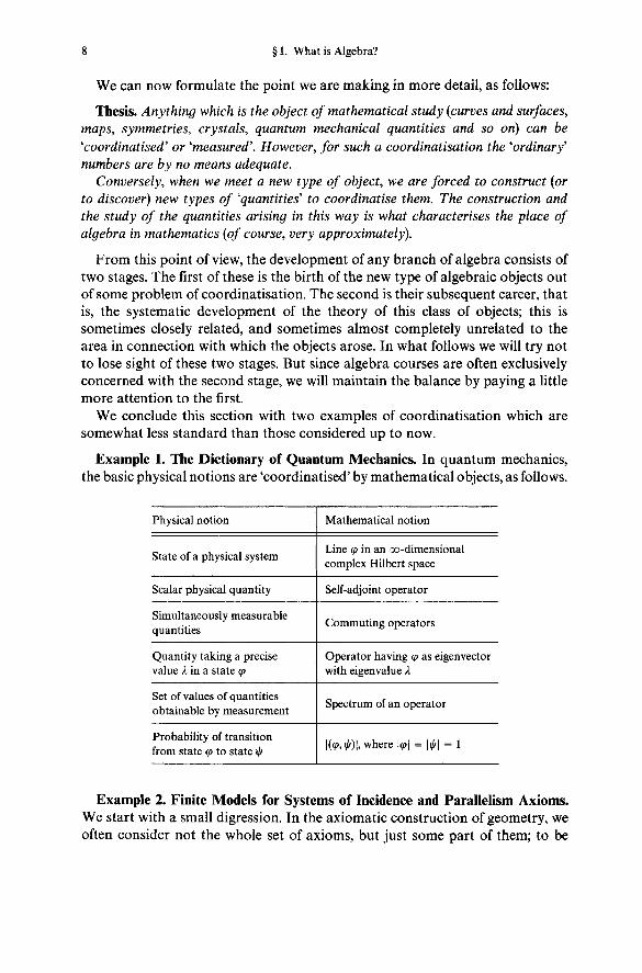
Example 1. The Dictionary of Quantum Mechanics. In quantum mechanics,the basic physical notions are 'coordinatised' by mathematical objects, as follows.

Physical notion

State of a physical system

Scalar physical quantity

Simultaneously measurablequantities

Quantity taking a precisevalue A in a state <p

Set of values of quantitiesobtainable by measurement

Probability of transitionfrom state q> to state i//

Mathematical notion

Line <p in an oo-dimensionalcomplex Hilbert space

Self-adjoint operator

Commuting operators

Operator having <p as eigenvectorwith eigenvalue X

Spectrum of an operator

|(«i»,^)|, where |<i()| = |^ | = l

Example 2. Finite Models for Systems of Incidence and Parallelism Axioms.We start with a small digression. In the axiomatic construction of geometry, weoften consider not the whole set of axioms, but just some part of them; to be

§1. What is Algebra?

B

G

A

^ \V

H

8 c

F

I

Fig. 1 Fig. 2

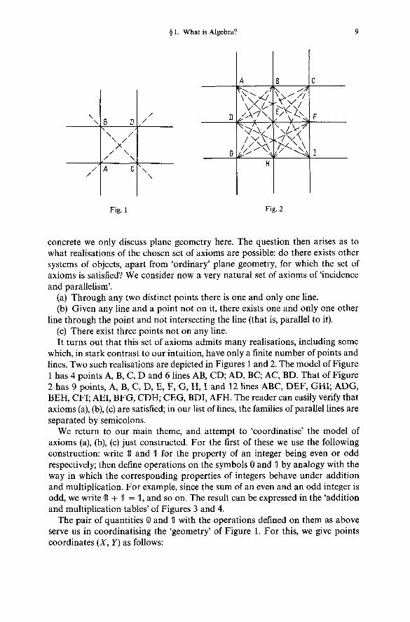
concrete we only discuss plane geometry here. The question then arises as towhat realisations of the chosen set of axioms are possible: do there exists othersystems of objects, apart from 'ordinary' plane geometry, for which the set ofaxioms is satisfied? We consider now a very natural set of axioms of 'incidenceand parallelism'.

(a) Through any two distinct points there is one and only one line.(b) Given any line and a point not on it, there exists one and only one other

line through the point and not intersecting the line (that is, parallel to it).(c) There exist three points not on any line.It turns out that this set of axioms admits many realisations, including some

which, in stark contrast to our intuition, have only a finite number of points andlines. Two such realisations are depicted in Figures 1 and 2. The model of Figure1 has 4 points A, B, C, D and 6 lines AB, CD; AD, BC; AC, BD. That of Figure2 has 9 points, A, B, C, D, E, F, G, H, I and 12 lines ABC, DEF, GHI; ADG,BEH, CFI; AEI, BFG, CDH; CEG, BDI, AFH. The reader can easily verify thataxioms (a), (b), (c) are satisfied; in our list of lines, the families of parallel lines areseparated by semicolons.

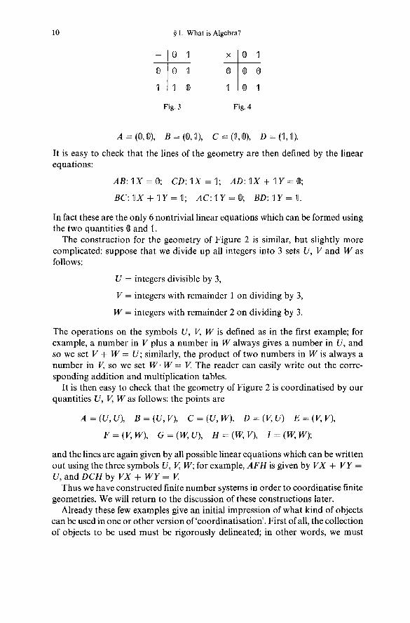
We return to our main theme, and attempt to 'coordinatise' the model ofaxioms (a), (b), (c) just constructed. For the first of these we use the followingconstruction: write 0 and 1 for the property of an integer being even or oddrespectively; then define operations on the symbols ffl and 11 by analogy with theway in which the corresponding properties of integers behave under additionand multiplication. For example, since the sum of an even and an odd integer isodd, we write 0 + 11 =11, and so on. The result can be expressed in the 'additionand multiplication tables' of Figures 3 and 4.

The pair of quantities © and 11 with the operations defined on them as aboveserve us in coordinatising the 'geometry' of Figure 1. For this, we give pointscoordinates (X, Y) as follows:

10

+i

1

§1.

©

©

11

What is Algebra

1 X

1 i

e n

?

© 1

© ©

i 11

Fig. 3 Fig. 4

It is easy to check that the lines of the geometry are then defined by the linearequations:

ABAX = ®; CD-AX = V, AD: HAT + 1 Y = i;

BC: I X + 17 = 1; AC: 11 7 = ©; BD: 117 = 1.

In fact these are the only 6 nontrivial linear equations which can be formed usingthe two quantities © and 11.

The construction for the geometry of Figure 2 is similar, but slightly morecomplicated: suppose that we divide up all integers into 3 sets U, V and W asfollows:

U = integers divisible by 3,

V = integers with remainder 1 on dividing by 3,

W = integers with remainder 2 on dividing by 3.

The operations on the symbols U, V, W is defined as in the first example; forexample, a number in V plus a number in W always gives a number in U, andso we set V + W = U; similarly, the product of two numbers in W is always anumber in V, so we set WW = V. The reader can easily write out the corre-sponding addition and multiplication tables.

It is then easy to check that the geometry of Figure 2 is coordinatised by ourquantities U, V, W as follows: the points are

A = (U,U), B = (U,V), C = (V,W), D = (V,U) E = (V,V),

and the lines are again given by all possible linear equations which can be writtenout using the three symbols U, V, W; for example, AFH is given by VX + VY =U, and DCH by VX + WY = V.

Thus we have constructed finite number systems in order to coordinatise finitegeometries. We will return to the discussion of these constructions later.

Already these few examples give an initial impression of what kind of objectscan be used in one or other version of'coordinatisation'. First of all, the collectionof objects to be used must be rigorously delineated; in other words, we must

§2. Fields 11

indicate a set (or perhaps several sets) of which these objects can be elements.Secondly, we must be able to operate on the objects, that is, we must defineoperations, which from one or more elements of the set (or sets) allow us toconstruct new elements. For the moment, no further restrictions on the nature ofthe sets to be used are imposed; in the same way, an operation may be a com-pletely arbitrary rule taking a set of k elements into a new element. All the same,these operations will usually preserve some similarities with operations onnumbers. In particular, in all the situations we will discuss, k = 1 or 2. The basicexamples of operations, with which all subsequent constructions should becompared, will be: the operation a t-+ — a taking any number to its negative; theoperation 61—> b"1 taking any nonzero number b to its inverse (for each of thesek = 1); and the operations (a, b)v->a + b and ab of addition and multiplication(for each of these k = 2).

§2. Fields

We start by describing one type of 'sets with operations' as described in § 1which corresponds most closely to our intuition of numbers.

A field is a set K on which two operations are defined, each taking two elementsof K into a third; these operations are called addition and multiplication, and theresult of applying them to elements a and b is denoted by a + b and ab. Theoperations are required to satisfy the following conditions:

Addition:Commutativity: a + b = b + a;Associativity: a + (b + c) = (a + b) + c;Existence of zero: there exists an element 0 e K such that a + 0 = a for every

a (it can be shown that this element is unique);Existence of negative: for any a there exists an element ( — a) such that

a + (— a) = 0 (it can be shown that this element is unique).Multiplication:

Commutativity: ab = ba;Associativity: a(bc) = (ab)c;Existence of unity: there exists an element 1 e K such that a\ = a for every a

(it can be shown that this element is unique);Existence of inverse: for any a / 0 there exists an element a~J such that

aa'1 = 1 (it can be shown that for given a, this element is unique).Addition and multiplication:

Distributivity: a(b + c) = ab + ac.Finally, we assume that a field does not consist only of the element 0, or

equivalently, that 0 # 1.

12 §2. Fields

These conditions taken as a whole, are called the field axioms. The ordinaryidentities of algebra, such as

(a + bf = a2 + lab + b2

or

a"1 -(a+ I)"1 = a " 1 ( a + l ) ~ 1

follow from the field axioms. We only have to bear in mind that for a naturalnumber n, the expression na means a + a + ••• + a (n times), rather than theproduct of a with the number n (which may not be in K).

Working over an arbitrary field K (that is, assuming that all coordinates,coefficients, and so on appearing in the argument belong to K) provides the mostnatural context for constructing those parts of linear algebra and analyticgeometry not involving lengths, polynomial algebras, rational fractions, andso on.

Basic examples of fields are the field of rational numbers, denoted by Q, thefield of real numbers U and the field of complex numbers C

If the elements of a field K are contained among the elements of a field L andthe operations in K and L agree, then we say that K is a subfield of L, and L anextension ofK, and we write K a L. For example, Q c R c C .

Example 1. In § 1, in connection with the 'geometry' of Figure 1, we definedoperations of addition and multiplication on the set {0,1}. It is easy to checkthat this is a field, in which i is the zero element and 1 the unity. If we write 0for (D) and 1 for 11, we see that the multiplication table of Figure 4 is just the rulefor multiplying 0 and 1 in <Q, and the addition table of Figure 3 differs in that1 + 1 = 0 . The field constructed in this way consisting of 0 and I is denoted byF2. Similarly, the elements U, V, W considered in connection with the geometryof Figure 2 also form a field, in which U = 0, V = 1 and W = — 1. We thus obtainexamples of fields with a finite number (2 or 3) of elements. Fields having onlyfinitely many elements (that is, finite fields) are very interesting objects with manyapplications. A finite field can be specified by writing out the addition andmultiplication tables of its elements, as we did in Figures 3-4. In § 1 we met suchfields in connection with the question of the realisation of a certain set of axiomsof geometry in a finite set of objects; but they arise just as naturally in algebraas realising the field axioms in a finite set of objects. A field consisting of qelements is denoted by ¥q.

Example 2. An algebraic expression obtained from an unknown x and arbi-trary elements of a field K using the addition, multiplication and division opera-tions, can be written in the form

ao + a1x + --- + anx"

b + bX + -- + bxm' U

where at,bteK and not all bt = 0. An expression of this form is called a rational

§2. Fields 13

fraction, or a rational function of x. We can now consider it as a function, takingany x in K (or any x in L, for some field L containing K) into the given expression,provided only that the denominator is not zero. All rational functions form afield, called the rational function field; it is denoted by K(x). We will discusscertain difficulties connected with this definition in § 3. The elements of K arecontained among the rational functions as 'constant' functions, so that K(x) isan extension of K.

In a similar way we define the field K(x, y) of rational functions in twovariables, or in any number of variables.

An isomorphism of two fields K' and K" is a 1-to-l correspondence a' <-*a"between their elements such that a' *->a" and b'<->£>" implies that a' + b' *-*a" + b" and a'b <->a"fo"; we say that two fields are isomorphic if there exists anisomorphism between them. If L' and L" are isomorphic fields, both of which areextensions of the same field K, and if the isomorphism between them takes eachelement of K into itself, then we say that it is an isomorphism over K, and thatL' and L" are isomorphic over K. An isomorphism of fields K' and K" is denotedby K' s K". If L' and L" are finite fields, then to say that they are isomorphicmeans that their addition and multiplication tables are the same; that is, theydiffer only in the notation for the elements of L' and L". The notion ofisomorphism for arbitrary fields is similar in meaning.

For example, suppose we take some line a and mark a point 0 and a 'unitinterval' OE on it; then we can in a geometric way define addition and multiplica-tion on the directed intervals (or vectors) contained in a. Their construction isgiven in Figures 5-6. In Figure 5, b is an arbitrary line parallel to a and U anarbitrary point on it, OU\\AV and VC\\ UB; then OC = OA + OB. In Figure 6,b is an arbitrary line passing through O, and EU \\ BV and VC || UA; then OC =OA • OB.

Fig. 5 Fig. 6

With this definition of the operations, intervals of the line form a field P; toverify all the axioms is a sequence of nontrivial geometric problems. Taking eachinterval into a real number, for example an infinite decimal fraction (this is againa process of measurement!), we obtain an isomorphism between P and the realnumber field U.

14 §2. Fields

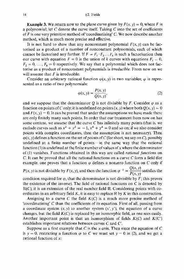
Example 3. We return now to the plane curve given by F(x, y) = 0, where F isa polynomial; let C denote the curve itself. Taking C into the set of coefficientsof F is one very primitive method of 'coordinatising' C. We now describe anothermethod, which is much more precise and effective.

It is not hard to show that any nonconstant polynomial F(x, y) can be fac-torised as a product of a number of nonconstant polynomials, each of whichcannot be factorised any further. If F = Fx • F2... Fk is such a factorisation thenour curve with equation F = 0 is the union of k curves with equations Ft = 0,F2 = 0, . . . , Fk = 0 respectively. We say that a polynomial which does not fac-torise as a product of nonconstant polynomials is irreducible. From now on wewill assume that F is irreducible.

Consider an arbitrary rational function <p(x,y) in two variables; q> is repre-sented as a ratio of two polynomials:

(p(xy) ——-,Q(x,y)

2)

and we suppose that the denominator Q is not divisible by F. Consider ipasafunction on points of C only; it is undefined on points (x, y) where both Q(x, y) = 0and F(x, y) = 0. It can be proved that under the assumptions we have made thereare only finitely many such points. In order that our treatment from now on hassome content, we assume that the curve C has infinitely many points (that is, weexclude curves such as x2 + y2 = — 1, x4 + y4 = 0 and so on; if we also considerpoints with complex coordinates, then the assumption is not necessary). Then(p(x, y) defines a function on the set of points of C (for short, we say on C), possiblyundefined at a finite number of points—in the same way that the rationalfunction (1) is undefined at the finite number of values of x where the denominatorof (1) vanishes. Functions obtained in this way are called rational functions onC. It can be proved that all the rational functions on a curve C form a field (forexample, one proves that a function cp defines a nonzero function on C only if

P(x, y) is not divisible by F(x, v), and then the function a>~1 = — satisfies theP(x,y)

condition required for cp, that the denominator is not divisible by F; this provesthe existence of the inverse). The field of rational functions on C is denoted byU(C); it is an extension of the real number field U. Considering points with co-ordinates in an arbitrary field K, it is easy to replace U by K in this construction.

Assigning to a curve C the field K(C) is a much more precise method of'coordinatising' C than the coefficients of its equation. First of all, passing froma coordinate system (x,y) to another system (x',y'\ the equation of a curvechanges, but the field K(C) is replaced by an isomorphic field, as one sees easily.Another important point is that an isomorphism of fields K(C) and K(C)establishes important relations between curves C and C.

Suppose as a first example that C is the x-axis. Then since the equation of Cis y = 0, restricting a function cp to C we must set y = 0 in (2), and we get arational function of x:

§2. Fields 15

P(x,O)<p(x,O) =

Q(x,oy

Thus in this case, the field K(C) is isomorphic to the rational function fieldK(x). Obviously, the same thing holds if C is an arbitrary line.

We proceed to the case of a curve C of degree 2. Let us prove that in this casealso the field K(C) is isomorphic to the field of rational functions of one variableK(t). For this, choose an arbitrary point (xo,yo) on C and take t to be the slopeof the line joining it to a point (x,y) with variable coordinates (Figure 7).

Fig. 7

y — yoIn other words, set t = , as a function on C. We now prove that x and

x - x0

y, as functions on C, are rational functions of t. For this, recall that y — y0 =t(x — x0), and if F(x, y) = 0 is the equation of C, then on C we have

F(x,yo + t(x-xo)) = O. (3)

In other words, the relation (3) is satisfied in K(C). Since C is a curve of degree2, this is a quadratic equation for x: a(t)x2 + b(t)x + c(t) = 0 (whose coefficientsinvolve t). However, one root of this equation is known, namely x = x0; thissimply reflects the fact that {xo,yo) is a point of C. The second root is then

b(t)obtained from the condition that the sum of the roots equals —. We get

a(t)an expression x = fit) as a rational function of t, and a similar expressiony = git); of course, F(/(t), gf(t)) = 0. Thus taking x <->/(£), y<-+g{t) and(pix,y)<-^xpifit),git)), we obtain an isomorphism of KiQ and X(t) over K.

The geometric meaning of the isomorphism obtained in this way is that pointsof C can be parametrised by rational functions: x = fit), y = gjt). If C hasthe equation y2 = ax2 + bx + c then on C we have y = ^Jax2 + bx + c, andanother form of the result we have obtained is that both x and Jax2 + bx + ccan be expressed as rational functions of some third function t. This expressionis useful, for example, in evaluating indeterminate integrals: it shows that any

16 §2. Fields

integralr

(p(x,y/ax2 + bx + c)dx,J

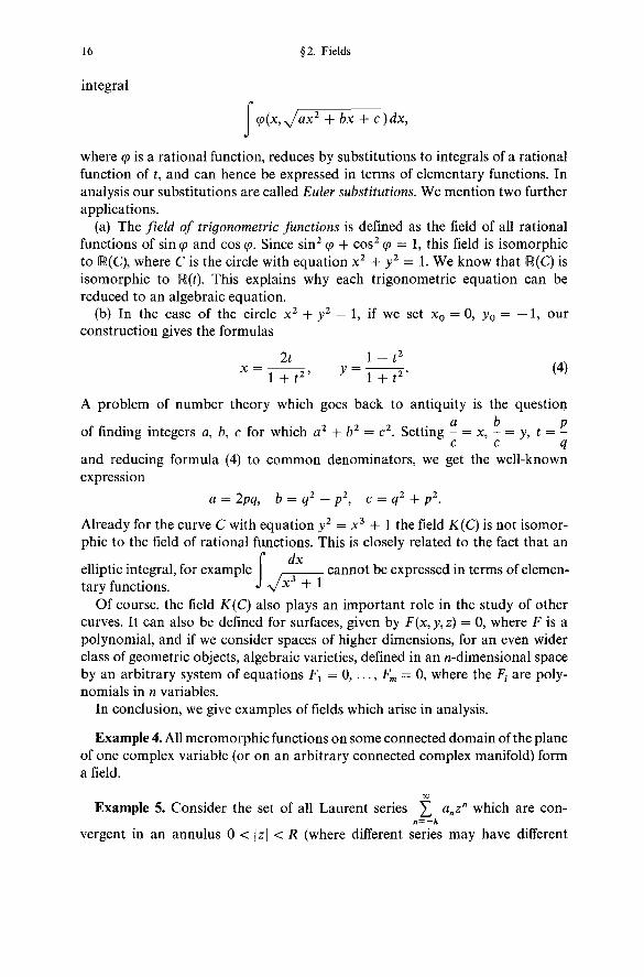
where (p is a rational function, reduces by substitutions to integrals of a rationalfunction of t, and can hence be expressed in terms of elementary functions. Inanalysis our substitutions are called Euler substitutions. We mention two furtherapplications.

(a) The field of trigonometric functions is defined as the field of all rationalfunctions of sin cp and cos cp. Since sin2 q> + cos2 cp = 1, this field is isomorphicto U(Q, where C is the circle with equation x2 + y2 = 1. We know that R(C) isisomorphic to U(t). This explains why each trigonometric equation can bereduced to an algebraic equation.

(b) In the case of the circle x2 + y2 = 1, if we set x0 = 0, y0 = — 1, ourconstruction gives the formulas

_ 2t _ ! - f 2

x — - =•, v —± -r I 1 T I

A problem of number theory which goes back to antiquity is the question

of finding integers a, b, c for which a2 + b2 = c2. Setting - = x, - = y, t = -c c q

and reducing formula (4) to common denominators, we get the well-knownexpression

a = 2pq, b = q2 — p2, c = q2 + p2.

Already for the curve C with equation y2 = x3 + 1 the field K(C) is not isomor-phic to the field of rational functions. This is closely related to the fact that an

f A

elliptic integral, for example cannot be expressed in terms of elemen-tary functions. J V31 + *

Of course, the field K(C) also plays an important role in the study of othercurves. It can also be defined for surfaces, given by F(x, y, z) = 0, where F is apolynomial, and if we consider spaces of higher dimensions, for an even widerclass of geometric objects, algebraic varieties, defined in an n-dimensional spaceby an arbitrary system of equations F1 = 0 , . . . , Fm = 0, where the Ft are poly-nomials in n variables.

In conclusion, we give examples of fields which arise in analysis.

Example 4. All meromorphic functions on some connected domain of the planeof one complex variable (or on an arbitrary connected complex manifold) forma field.

00

Example 5. Consider the set of all Laurent series £ anz" which are con-n=-k

vergent in an annul us 0 < \z\ < R (where different series may have different

§3. Commutative Rings 17

annuluses of convergence). With the usual definition of operations on series, theseform a field, the field of Laurent series. If we use the same rules to compute thecoefficients, we can define the sum and product of two Laurent series, even ifthese are nowhere convergent. We thus obtain the field of formal Laurent series.One can go further, and consider this construction in the case that the coefficientsan belong to an arbitrary field K. The resulting field is called the field of formalLaurent series with coefficients in K, and is denoted by K((z)).

§ 3. Commutative Rings

The simplest possible example of 'coordinatisation' is counting, and it leads(once 0 and negative numbers have been introduced) to the integers, which donot form a field. Operations of addition and multiplication are defined on theset of all integers (positive, zero or negative), and these satisfy all the field axiomsbut one, namely the existence of an inverse element a"1 for every a # 0 (since,for example, j is already not an integer).

A set having two operations, called addition and multiplication, satisfying allthe field axioms except possibly for the requirement of existence of an inverseelement a"1 for every a # 0 is called a commutative ring; it is convenient not toexclude the ring consisting just of the single element 0 from the definition.

The field axioms, with the axiom of the existence of an inverse and thecondition 0 # 1 omitted will from now on be referred to as the commutative ringaxioms.

By analogy with fields, we define the notions of a subring A a B of a ring, andisomorphism of two rings A' and A"; in the case that A c A' and A <= A" we alsohave the notion of an isomorphism of A' and A" over A; an isomorphism of ringsis again written A' = A".

Example 1. The Ring of Integers. This is denoted by Z; obviously Z c Q .

Example 2. An example which is just a fundamental is the polynomial ringA[x] with coefficients in a ring A. In view of its fundamental role, we spend sometime on the detailed definition of A[x]. First we characterise it by certainproperties.

We say that a commutative ring B is a polynomial ring over a commutativering A if B => A and B contains an element x with the property that every elementof B can be uniquely written in the form

a0 + a1x + ••• + anx" with at e A

for some n ^ 0. If B' is another such ring, with x' the corresponding element, thecorrespondence

18 §3. Commutative Rings

a0 + a^x + • • • + anx" <-> a0 + axx' + h an(x')n

defines an isomorphism of B and B' over A, as one sees easily. Thus the poly-nomial ring is uniquely defined, in a reasonable sense.

However, this does not solve the problem as to its existence. In most cases the'functional' point of view is sufficient: we consider the functions f of A into itselfof the form

f(c) = a0 + axc + ••• + anc" for c e A. (1)

Operations on functions are defined as usual: ( / + g){c) = /(c) + g(c) and(fd)(c) = fic)g{c). Taking an element ae A into the constant function f(c) = a,we can view A as a subring of the ring of functions. If we let x denote the functionx(c) = c then the function (1) is of the form

f = a0 + aix + --- + anxn. (2)

However, in some cases (for example if the number of elements of A is finite, andn is greater than this number), the expression (2) for / may not be unique. Thusin the field F2 of §2, Example 1, the functions x and x2 are the same. For thisreason we give an alternative construction.

We could define polynomials as 'expressions' a0 + a1x + ••• + anx", with +and x' thought of as conventional signs or place-markers, serving to denote thesequence (ao,...,an) of elements of a field K. After this, sum and product aregiven by formulas

£ cmxm where cm= £ akbt.m k+l=m

Rather more concretely, the same idea can be formulated as follows. We considerthe set of all infinite sequences (a0, a1,.. .,an,...) of elements of a ring A, everysequence consisting of zeros from some term onwards (this term may be differentfor different sequences). First we define addition of sequences by

(aQ,a1,...,an,...) + {b0,bu...,bn,...) = (a0 + foo,«i + bu...,an +bn,...).

All the ring axioms concerning addition are satisfied. Now for multiplication wedefine first just the multiplication of sequences by elements of A:

a(a0, a1,...,an,...) = (aao,aau..., aan,...).

We write Ek = (0,.. . , 1,0,...) for the sequence consisting of 1 in the /cth placeand 0 everywhere else. Then it is easy to see that

{ao,au...,an,...)= £ akEk. (3)

§3. Commutative Rings 19

Here the right-hand side is a finite sum in view of the condition imposed onsequences. Now define multiplication by

) |>A£*+, (4)

(on the right-hand side we must gather together all the terms for k and / withk + I = n as the coefficient of En). It follows from (4) that Eo is the unit elementof the ring, and Ek = E\. Setting Ey = x we can write the sequence (3) in the formYjak

xk- Obviously this expression for the sequence is unique. It is easy to checkthat the multiplication (4) satisfies the axioms of a commutative ring, so that thering we have constructed is the polynomial ring >l[x].

The polynomial ring /l[x,_y] is defined as -4[x][.y], or by generalising theabove construction. In a similar way one defines the polynomial ring A[xu... ,xn~\in any number of variables.

Example 3. All linear differential operators with constant (real) coefficients can8 8

be written as polynomials in the operators -—, . . . , -—. Hence they form a ringdXi dxn

Sending -— to tt defines an isomorphism

r d d n\_8xl'""dxn]'

orphism

V d d 1I ______ i ^ o r*- *• ~i

\_8x1'""'dxn]~If A = K is a field then the polynomial ring K [x] is a subring of the rational

function field K(x), in the same way that the ring of integers Z is a subring of therational field Q. A ring which is a subring of a field has an important property:the relation ab = 0 is only possible in it if either a = 0 or b = 0; indeed, it followseasily from the commutative ring axioms that a • 0 = 0 for any a. Hence if ab = 0in a field and a / 0, multiplying on the left by a"1 gives 6 = 0. Obviously thesame thing holds for a ring contained in a field.

A commutative ring with the properties that for any of its elements a, b theproduct ab = 0 only if a = 0 or b = 0, and that 0 # 1, is called an integral ringor an integral domain. Thus a subring of any field is an integral domain.

Theorem I. For any integral domain A, there exists a field K containing A as asubring, and such that every element of K can be written in the form ab'1 witha,beA and b # 0. A field K with this property is called the field of fractions ofA; it is uniquely defined up to isomorphism.

For example, the field of fractions of Z is Q, that of the polynomial ring .K[x]is the field of rational functions K(x), and that of K\^x1,.. . ,xn] is X(x l 5 . . . ,xn).Quite generally, fields of fractions give an effective method of constructing newfields.

20 § 3. Commutative Rings

Example 4. If A and B are two rings, their direct sum is the ring consisting ofpairs (a, b) with ae A and b e B, with addition and multiplication give by

(aub1) + (a2,b2) = (aj + a2,bx + b2),

Direct sum is denoted by A © B. The direct sum of any number of rings is definedin a similar way.

A direct sum is not an integral domain: (a,0)(0, b) = (0,0), which is the zeroelement of A © B.

The most important example of commutative rings, which includes non-integral rings, is given by rings of functions. Properly speaking, the direct sumA © • • • © A of n copies of A can be viewed as the ring of function on a set ofn elements (such as {1,2,...,n}) with values in A: the element (a 1 , . . . ,a n)eA © • • • © A can be identified with the function / given by f(i) = at. Additionand multiplication of functions are given as usual by operating on their values.

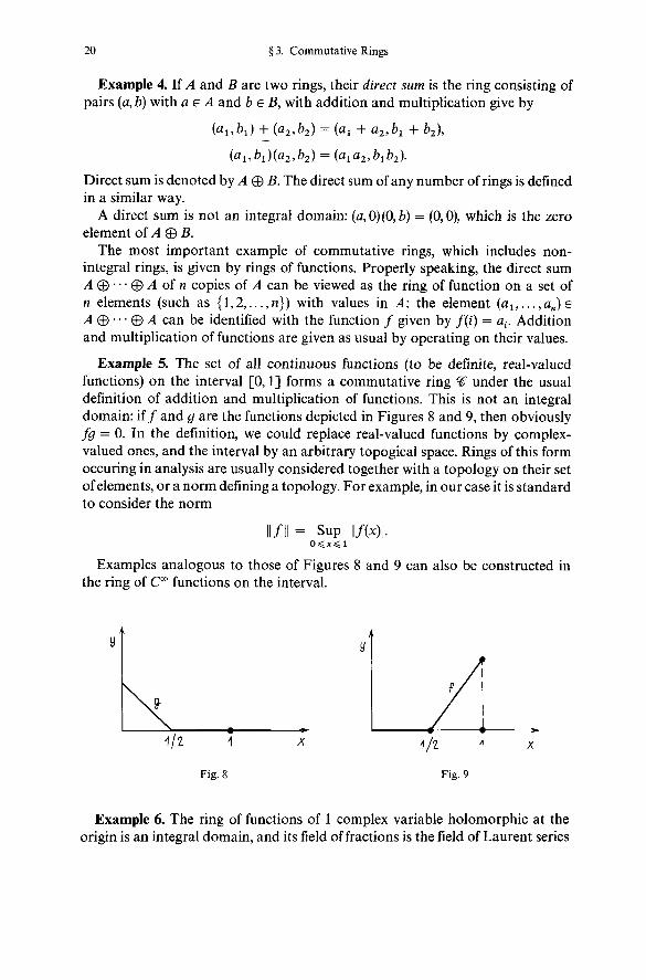
Example 5. The set of all continuous functions (to be definite, real-valuedfunctions) on the interval [0,1] forms a commutative ring ^ under the usualdefinition of addition and multiplication of functions. This is not an integraldomain: if/ and g are the functions depicted in Figures 8 and 9, then obviouslyfg = 0. In the definition, we could replace real-valued functions by complex-valued ones, and the interval by an arbitrary topogical space. Rings of this formoccuring in analysis are usually considered together with a topology on their setof elements, or a norm defining a topology. For example, in our case it is standardto consider the norm

| | / | | = Sup |/(x)|.

Examples analogous to those of Figures 8 and 9 can also be constructed inthe ring of C* functions on the interval.

-1/2 1 X

Fig. 8 Fig. 9

Example 6. The ring of functions of 1 complex variable holomorphic at theorigin is an integral domain, and its field of fractions is the field of Laurent series

§3. Commutative Rings 21

(§ 2, Example 5). Similarly to § 2, Example 5 we can define the ring of formal power

series £ ant" with coefficients an in any field K. This can also be constructedn = 0

as in Example 2, if we just omit the condition that the sequences (a0, a1,...,an,...)are 0 from some point onwards. This is also an integral domain, and its field offractions is the field of formal Laurent series K((t)). The ring of formal powerseries is denoted by Kit}.

Example 7. The ring &„ of functions in n complex variables holomorphic at theorigin, that is of functions that can be represented as power series

convergent in some neighbourhood of the origin. By analogy with Example 6we can define the rings of formal power series C[z 1 ; . . . ,z n ] with complex coef-ficients, and K \_zv,..., zB] with coefficients in any field K.

Example 8. We return to the curve C defined in the plane by the equationF(x, y) = 0, where F is a polynomial with coefficients in a field K, as consideredin § 2. With each polynomial P(x, y) we associate the function on the set of pointsof C defined by restricting P to C. Functions of this form are polynomial functionson C. Obviously they form a commutative ring, which we denote by K[C]. If Fis a product of factors then the ring K [C] may not be an integral domain. Forexample if F = xy then C is the union of the coordinate axes; then x is zero onthe y-axis, and y on the x-axis, so that their product is zero on the whole curveC. However, if F is an irreducible polynomial then K [C] is an integral domain.In this case the field of fractions of K[C] is the rational function field K(C) of C;the ring fc[C] is called the coordinate ring of C.

Taking an algebraic curve C into the ring X[C] is also an example of'coordinatisation', and in fact is more precise than taking C to K{C), since X[C]determines K(C) (as its field of fractions), whereas there exist curves C and C forwhich the fields K(C) and K(C) are isomorphic, but the rings K[_C\ and K[_C]are not.

Needless to say, we could replace the algebraic curve given by F(x, y) = 0 byan algebraic surface given by F(x,y, z) — 0, and quite generally by an algebraicvariety.

Example 9. Consider an arbitrary set M, and the commutative ring A con-sisting of all functions on M with values in the finite field with two elements F2

(§2, Example 1). Thus A consists of all maps from M to F2. Since F2 has only twoelements 0 and 1, a function with values in F2 is uniquely determined by the subset[ / c M o f elements on which it takes the value 1 (on the remainder it takes thevalue 0). Conversely, any subset [ J c M determines a function q>v with <pv{m) = 1if me U and cpv(m) = 0 if m $ U. It is easy to see which operations on subsetscorrespond to the addition and multiplication of functions:

<Pu-(Pv = Vvnv a n d <Pv + <Pv =

22 § 3. Commutative Rings

where U A V is the symmetric difference, U A V = (U u V) \ (U nV). Thus ourring can be described as being made up of subsets 1 / c F with the operations ofsymmetric difference and intersection as sum and product. This ring was in-troduced by Boole as a formal notation for assertions in logic. Since x2 = x forevery element of F2, this relations holds for any function with values in F2, thatis, it holds in A. A ring for which every element x satisfies x2 = x is a Boolean ring.

More general examples of Boolean rings can be constructed quite similarly,by taking not all subsets of M, but only some system S of subsets containingtogether with U and V the subsets U n V and U u F , and together with U itscomplement. For example, we could consider a topological space having theproperty that every open set is also closed (such a space is called 0-dimensional\and let S be the set of open subsets of M. It can be proved that every Booleanring can be obtained in this way. In the following section § 4 we will indicate theprinciple on which the proof of this is based.

The qualitatively new phenomenon that occurs on passing from fields toarbitrary commutative rings is the appearance of a nontrivial theory of divisi-bility. An element a of a ring A is divisible by an element b if there exists c in Asuch that a = be. A field is precisely a ring in which the divisibility theory istrivial: any element is divisible by any nonzero element, since a = b(ab~x). Theclassical example of divisibility theory is the theory of divisibility in the ring Z:this was constructed already in antiquity. The basic theorem of this theory is thefact that any integer can be uniquely expressed as a product of prime factors.The proof of this theorem, as is well known, is based on division with remainder(or the Euclidean algorithm).

Let A be an arbitrary integral domain. We say that an element a e A isinvertible or is a unit of A if it has an inverse in A; in Z the units are + 1, in K[x]

CO

the nonzero constants c e K, and in KfxJ the series £ anx" with a0 ^ 0. Any;=o

element of A is divisible by a unit. An element a is said to be prime if its onlyfactorisations are of the form a = cic^a) where c is a unit. If an integral domainA has the property that every nonzero element can be written as a product ofprimes, and this factorisation is unique up to renumbering the prime factors andmultiplication by units, we say that A is a unique factorisation domain (UFD) ora factorial ring. Thus Z is a UFD, and so is K[x] (the proof uses division withremainder for polynomials). It can be proved that if A is a UFD then so is A [x];hence A[x1,..., xn] is also a UFD. The prime elements of a polynomial ring arecalled irreducible polynomials. In C [x] only the linear polynomials are irreduci-ble, and in R[x] only linear polynomials and quadratic polynomials having noreal roots. In Q [x] there are irreducible polynomials of any degree, for examplethe polynomial x" — p where p is any prime number.

Important examples of UFDs are the ring (9n of functions in n complexvariables holomorphic at the origin, and the formal power series ringK\tu...,t^ (Example 7). The proof that these are UFDs is based on theWeierstrass preparation theorem, which reduces the problem to functions (or

§ 3. Commutative Rings 23

formal power series) which are polynomials in one of the variables. After this,one applies the fact that A [t] is a UFD (provided A is) and an induction.

Example 10. The Gaussian Integers. It is easy to see that the complex numbersof the form m + ni, where m and n are integers, form a ring. This is a UFD, ascan also be proved using division with remainder (but the quantity that decreaseson taking the remainder is m2 + n2). Since in this ring

m2 + n2 = (m + ni)(m — ni),

divisibility in it can be used as the basis of the solution of the problem ofrepresenting integers as the sum of two squares.

Example 11. Let e be a (complex) root of the equation s2 + s + 1 = 0. Complexnumbers of the form m + ns, where m and n are integers, also form a ring, whichis also a UFD. In this ring the expression m3 + n3 factorises as a product:

m3 + n3 = (m + n)(m + ns)(m + ris),

where e" = e2 = — (1 + e) is the complex conjugate of e. Because of this, divisi-bility theory in this ring serves as the basis of the proof of Fermat's Last Theo-rem for cubes. The 18th century mathematicians Lagrange and Euler wereamazed to find that the proof of a theorem of number theory (the theory ofthe ring Z) can be based on introducing other numbers (elements of otherrings).

Example 12. We give an example of an integral domain which is not a UFD;this is the ring consisting of all complex numbers of the form m + n^J — 5 wherem, ne Z. Here is an example of two different factorisations into irreduciblefactors:

32 = (2

We need only check that 3, 2 + ^/ — 5 and 2 — v / — 5 are irreducible elements.For this, we write N(a) for the square of the absolute value of a; if a = n + m^J — 5then N(a) = (n + m^J — 5){n — m^f —5) = n2 + 5m2, which is a positive integer.Moreover, it follows from the properties of absolute value that N(a/i) =N(a)N{fi). If, say, 2 + > / ^ 5 is reducible, for example 2 + y/^-5 = aft, thenN(2 + v ^ 5 ) = N(a)N(fi). But N(2 + ^^5) = 9, and hence there are only threepossibilities: (N(a), N(fi)) = (3,3) or (1,9) or (9,1). The first of these is impossible,since 3 cannot be written in the form n2 + 5m2 with n, m integers. In the secondP = +1 and in the third a = ± 1, so a or ft is a unit. This proves that 2 + ^/— 5is irreducible.

To say that a ring is not a UFD does not mean to say that it does not havean interesting theory of divisibility. On the contrary, in this case the theory ofdivisibility becomes especially interesting. We will discuss this in more detail inthe following section § 4.

24 §4. Homomorphisms and Ideals

§ 4. Homomorphisms and Ideals

A further difference of principle between arbitrary commutative rings andfields is the existence of nontrivial homomorphisms. A homomorphism of a ringA to a ring £ is a map / : A ->• B such that

/ (a 1 +fl 2 )=/ (a 1 ) + /(a2), f{a1a2)=f(a1)-f(a2) and f(lA)=lB

(we write 1A and lB for the identity elements of A of B). An isomorphism is ahomomorphism having an inverse.

If a ring has a topology, then usually only continuous homomorphisms are ofinterest.

Typical examples of homomorphisms arise if the rings A and B are realised asrings of functions on sets X and Y (for example, continuous, differentiable oranalytic functions, or polynomial functions on an algebraic curve C). A mapq>: Y -* X transforms a function F on X into the function q>*F on Y defined bythe condition

(cp*F)(y) =

If cp satisfies the natural conditions for the theory under consideration (that is,if (p is a continuous, differentiable or analytic map, or is given by polynomialexpressions) then <p* defines a homomorphism of A to B. The simplest particu-lar case is when cp is an embedding, that is Y is a subset of X. Then q>* is simplythe resjriction to Y of functions defined on X.

Example 1. If C is a curve, defined by the equation F(x, y) = 0 whereF e K[x, y] is an irreducible polynomial, then restriction to C defines a homo-morphism K[x,y] -> K[C].

The case which arises most often is when Y is one point of a set X, that isY = {x0} with x0 e X; then we are just evaluating a function, taking it into itsvalue at x0.

Example 2. If x0 e C then taking each function of K\_C] into its value at x0

defines a homomorphism K [C] -> K.

Example 3. If t? is the ring of continuous functions on [0,1] and x0 e [0,1]then taking a function q> e %> into its value cp(x0) is a homomorphism %? -» R. IfA is the ring of functions which are holomorphic in a neighbourhood of 0, thentaking <p e A into its value q>(0) is a homomorphism A-+C.

Interpreting the evaluation of a function at a point as a homomorphism hasled to a general point of view on the theory of rings, according to which acommutative ring can very often be interpreted as a ring of functions on a set,the 'points' of which correspond to homomorphisms of the original ring intofields. The original example is the ring X[C], where C is an algebraic variety,and from it, the geometric intuition spreads out to more general rings. Thusthe concept that 'every geometric object can be coordinatised by some ring of