encyclopaedia of mathematical sciences volume 122 operator
TRANSCRIPT

Encyclopaedia of Mathematical SciencesVolume 122
Operator Algebras and Non-Commutative Geometry III
Subseries Editors:Joachim Cuntz Vaughan F.R. Jones

B. Blackadar
Operator AlgebrasTheory of C∗-Algebras
and von NeumannAlgebras
ABC

Bruce BlackadarDepartment of MathematicsUniversity of Nevada, Reno
Reno, NV 89557USA
e-mail: [email protected]
Founding editor of the Encyclopedia of Mathematical Sciences:R. V. Gamkrelidze
Library of Congress Control Number: 2005934456
Mathematics Subject Classification (2000):46L05, 46L06, 46L07, 46L08, 46L09, 46L10, 46L30, 46L35, 46L40, 46L45, 46L51,
46L55, 46L80, 46L85, 46L87, 46L89, 19K14, 19K33
ISSN 0938-0396ISBN-10 3-540-28486-9 Springer Berlin Heidelberg New York
ISBN-13 978-3-540-28486-4 Springer Berlin Heidelberg New York
This work is subject to copyright. All rights are reserved, whether the whole or part of the material isconcerned, specifically the rights of translation, reprinting, reuse of illustrations, recitation, broadcasting,reproduction on microfilm or in any other way, and storage in data banks. Duplication of this publication
or parts thereof is permitted only under the provisions of the German Copyright Law of September 9,1965, in its current version, and permission for use must always be obtained from Springer. Violations
are liable for prosecution under the German Copyright Law.
Springer is a part of Springer Science+Business Media
c© Springer-Verlag Berlin Heidelberg 2006Printed in Germany
The use of general descriptive names, registered names, trademarks, etc. in this publication does notimply, even in the absence of a specific statement, that such names are exempt from the relevant
protective laws and regulations and therefore free for general use.
Typesetting: by the author and TechBooks using a Springer LATEX macro package
Cover design: design & production GmbH, Heidelberg
Printed on acid-free paper SPIN: 11543510 46/TechBooks 5 4 3 2 1 0
springer.com

to my parentsand
in memory of Gert K. Pedersen

Preface to the Encyclopaedia Subserieson Operator Algebras and Non-Commutative
Geometry
The theory of von Neumann algebras was initiated in a series of papers byMurray and von Neumann in the 1930’s and 1940’s. A von Neumann algebrais a self-adjoint unital subalgebra M of the algebra of bounded operatorsof a Hilbert space which is closed in the weak operator topology. Accordingto von Neumann’s bicommutant theorem, M is closed in the weak operatortopology if and only if it is equal to the commutant of its commutant. A factoris a von Neumann algebra with trivial centre and the work of Murray and vonNeumann contained a reduction of all von Neumann algebras to factors anda classification of factors into types I, II and III.
C∗-algebras are self-adjoint operator algebras on Hilbert space which areclosed in the norm topology. Their study was begun in the work of Gelfandand Naimark who showed that such algebras can be characterized abstractlyas involutive Banach algebras, satisfying an algebraic relation connecting thenorm and the involution. They also obtained the fundamental result thata commutative unital C∗-algebra is isomorphic to the algebra of complexvalued continuous functions on a compact space – its spectrum.
Since then the subject of operator algebras has evolved into a huge math-ematical endeavour interacting with almost every branch of mathematics andseveral areas of theoretical physics.
Up into the sixties much of the work on C∗-algebras was centered aroundrepresentation theory and the study of C∗-algebras of type I (these algebrasare characterized by the fact that they have a well behaved representationtheory). Finite dimensional C∗-algebras are easily seen to be just direct sumsof matrix algebras. However, by taking algebras which are closures in norm offinite dimensional algebras one obtains already a rich class of C∗-algebras – theso-called AF-algebras – which are not of type I. The idea of taking the closureof an inductive limit of finite-dimensional algebras had already appeared in thework of Murray-von Neumann who used it to construct a fundamental exampleof a factor of type II – the ”hyperfinite” (nowadays also called approximatelyfinite dimensional) factor.

VIII Preface to the Subseries
One key to an understanding of the class of AF-algebras turned out tobe K-theory. The techniques of K-theory, along with its dual, Ext-theory,also found immediate applications in the study of many new examples ofC∗-algebras that arose in the end of the seventies. These examples includefor instance ”the noncommutative tori” or other crossed products of abelianC∗-algebras by groups of homeomorphisms and abstract C∗-algebras gener-ated by isometries with certain relations, now known as the algebras On. Atthe same time, examples of algebras were increasingly studied that codify datafrom differential geometry or from topological dynamical systems.
On the other hand, a little earlier in the seventies, the theory of von Neu-mann algebras underwent a vigorous growth after the discovery of a naturalinfinite family of pairwise nonisomorphic factors of type III and the adventof Tomita-Takesaki theory. This development culminated in Connes’ greatclassification theorems for approximately finite dimensional (“injective”) vonNeumann algebras.
Perhaps the most significant area in which operator algebras have beenused is mathematical physics, especially in quantum statistical mechanics andin the foundations of quantum field theory. Von Neumann explicitly mentionedquantum theory as one of his motivations for developing the theory of ringsof operators and his foresight was confirmed in the algebraic quantum fieldtheory proposed by Haag and Kastler. In this theory a von Neumann algebrais associated with each region of space-time, obeying certain axioms. Theinductive limit of these von Neumann algebras is a C∗-algebra which containsa lot of information on the quantum field theory in question. This point ofview was particularly successful in the analysis of superselection sectors.
In 1980 the subject of operator algebras was entirely covered in a singlebig three weeks meeting in Kingston Ontario. This meeting served as a re-view of the classification theorems for von Neumann algebras and the suc-cess of K-theory as a tool in C∗-algebras. But the meeting also containeda preview of what was to be an explosive growth in the field. The study ofthe von Neumann algebra of a foliation was being developed in the far moreprecise C∗-framework which would lead to index theorems for foliations incor-porating techniques and ideas from many branches of mathematics hithertounconnected with operator algebras.
Many of the new developments began in the decade following the Kingstonmeeting. On the C∗-side was Kasparov’s KK-theory – the bivariant form ofK-theory for which operator algebraic methods are absolutely essential. Cycliccohomology was discovered through an analysis of the fine structure of exten-sions of C∗-algebras These ideas and many others were integrated into Connes’vast Noncommutative Geometry program. In cyclic theory and in connectionwith many other aspects of noncommutative geometry, the need for going be-yond the class of C∗-algebras became apparent. Thanks to recent progress,both on the cyclic homology side as well as on the K-theory side, there isnow a well developed bivariant K-theory and cyclic theory for a natural classof topological algebras as well as a bivariant character taking K-theory to

Preface to the Subseries IX
cyclic theory. The 1990’s also saw huge progress in the classification theory ofnuclear C∗-algebras in terms of K-theoretic invariants, based on new insightinto the structure of exact C∗-algebras.
On the von Neumann algebra side, the study of subfactors began in 1982with the definition of the index of a subfactor in terms of the Murray-von Neu-mann theory and a result showing that the index was surprisingly restrictedin its possible values. A rich theory was developed refining and clarifyingthe index. Surprising connections with knot theory, statistical mechanics andquantum field theory have been found. The superselection theory mentionedabove turned out to have fascinating links to subfactor theory. The subfactorsthemselves were constructed in the representation theory of loop groups.
Beginning in the early 1980’s Voiculescu initiated the theory of free prob-ability and showed how to understand the free group von Neumann algebrasin terms of random matrices, leading to the extraordinary result that the vonNeumann algebra M of the free group on infinitelymany generators has fullfundamental group, i.e. pMp is isomorphic to M for every non-zero projec-tion p ∈ M . The subsequent introduction of free entropy led to the solutionof more old problems in von Neumann algebras such as the lack of a Cartansubalgebra in the free group von Neumann algebras.
Many of the topics mentioned in the (obviously incomplete) list above havebecome large industries in their own right. So it is clear that a conference likethe one in Kingston is no longer possible. Nevertheless the subject does retaina certain unity and sense of identity so we felt it appropriate and useful tocreate a series of encylopaedia volumes documenting the fundamentals of thetheory and defining the current state of the subject.
In particular, our series will include volumes treating the essential techni-cal results of C∗-algebra theory and von Neumann algebra theory includingsections on noncommutative dynamical systems, entropy and derivations. Itwill include an account of K-theory and bivariant K-theory with applicationsand in particular the index theorem for foliations. Another volume will bedevoted to cyclic homology and bivariant K-theory for topological algebraswith applications to index theorems. On the von Neumann algebra side, weplan volumes on the structure of subfactors and on free probability and freeentropy. Another volume shall be dedicated to the connections between oper-ator algebras and quantum field theory.
October 2001 subseries editors:Joachim CuntzVaughan Jones

Preface
This volume attempts to give a comprehensive discussion of the theory ofoperator algebras (C*-algebras and von Neumann algebras.) The volume isintended to serve two purposes: to record the standard theory in the Encyclo-pedia of Mathematics, and to serve as an introduction and standard referencefor the specialized volumes in the series on current research topics in thesubject.
Since there are already numerous excellent treatises on various aspects ofthe subject, how does this volume make a significant addition to the literature,and how does it differ from the other books in the subject? In short, whyanother book on operator algebras?
The answer lies partly in the first paragraph above. More importantly,no other single reference covers all or even almost all of the material in thisvolume. I have tried to cover all of the main aspects of “standard” or “classi-cal” operator algebra theory; the goal has been to be, well, encyclopedic. Ofcourse, in a subject as vast as this one, authors must make highly subjectivejudgments as to what to include and what to omit, as well as what level ofdetail to include, and I have been guided as much by my own interests andprejudices as by the needs of the authors of the more specialized volumes.
A treatment of such a large body of material cannot be done at the detaillevel of a textbook in a reasonably-sized work, and this volume would not besuitable as a text and certainly does not replace the more detailed treatmentsof the subject. But neither is this volume simply a survey of the subject (afine survey-level book is already available [Fil96].) My philosophy has been tonot only state what is true, but explain why: while many proofs are merelyoutlined or even omitted, I have attempted to include enough detail and ex-planation to at least make all results plausible and to give the reader a senseof what material and level of difficulty is involved in each result. Where an ar-gument can be given or summarized in just a few lines, it is usually included;longer arguments are usually omitted or only outlined. More detail has beenincluded where results are particularly important or frequently used in thesequel, where the results or proofs are not found in standard references, and

XII Preface
in the few cases where new arguments have been found. Nonetheless, through-out the volume the reader should expect to have to fill out compactly writtenarguments, or consult references giving expanded expositions.
I have concentrated on trying to give a clean and efficient exposition of thedetails of the theory, and have for the most part avoided general discussionsof the nature of the subject, its importance, and its connections and applica-tions in other parts of mathematics (and physics); these matters have beenamply treated in the introductory article to this series. See the introductionto [Con94] for another excellent overview of the subject of operator algebras.
There is very little in this volume that is truly new, mainly some simplifiedproofs. I have tried to combine the best features of existing expositions andarguments, with a few modifications of my own here and there. In preparingthis volume, I have had the pleasure of repeatedly reflecting on the outstandingtalents of the many mathematicians who have brought this subject to itspresent advanced state, and the theory presented here is a monument to theircollective skills and efforts.
Besides the unwitting assistance of the numerous authors who originallydeveloped the theory and gave previous expositions, I have benefited fromcomments, suggestions, and technical assistance from a number of other spe-cialists, notably G. Pedersen, N. C. Phillips, and S. Echterhoff, my colleaguesB.-J. Kahng, V. Deaconu, and A. Kumjian, and many others who set mestraight on various points either in person or by email. I am especially grate-ful to Marc Rieffel, who, in addition to giving me detailed comments on themanuscript, wrote an entire draft of Section II.10 on group C*-algebras andcrossed products. Although I heavily modified his draft to bring it in linewith the rest of the manuscript stylistically, elements of Marc’s vision andrefreshing writing style still show through. Of course, any errors or misstate-ments in the final version of this (and every other) section are entirely myresponsibility.
Speaking of errors and misstatements, as far-fetched as the possibilitymay seem that any still remain after all the ones I have already fixed, I wouldappreciate hearing about them from readers, and I plan to post whatever Ifind out about on my website.
No book can start from scratch, and this book presupposes a level ofknowledge roughly equivalent to a standard graduate course in functionalanalysis (plus its usual prerequisites in analysis, topology, and algebra.) Inparticular, the reader is assumed to know such standard theorems as the Hahn-Banach Theorem, the Krein-Milman Theorem, and the Riesz RepresentationTheorem (the Open Mapping Theorem, the Closed Graph Theorem, and theUniform Boundedness Principle also fall into this category but are explicitlystated in the text sinced they are more directly connected with operator theoryand operator algebras.) Most of the likely readers will have this background,or far more, and indeed it would be difficult to understand and appreciate thematerial without this much knowledge. Beginning with a quick treatment ofthe basics of Hilbert space and operator theory would seem to be the proper

Preface XIII
point of departure for a book of this sort, and the early sections will be usefuleven to specialists to set the stage for the work and establish notation andterminology.
September 2005 Bruce Blackadar

Contents
I Operators on Hilbert Space . . . . . . . . . . . . . . . . . . . . . . . . . . . . . . . . 1I.1 Hilbert Space . . . . . . . . . . . . . . . . . . . . . . . . . . . . . . . . . . . . . . . . . 1
I.1.1 Inner Products . . . . . . . . . . . . . . . . . . . . . . . . . . . . . . . 1I.1.2 Orthogonality . . . . . . . . . . . . . . . . . . . . . . . . . . . . . . . 2I.1.3 Dual Spaces and Weak Topology . . . . . . . . . . . . . . . 3I.1.4 Standard Constructions . . . . . . . . . . . . . . . . . . . . . . . 4I.1.5 Real Hilbert Spaces . . . . . . . . . . . . . . . . . . . . . . . . . . 5
I.2 Bounded Operators . . . . . . . . . . . . . . . . . . . . . . . . . . . . . . . . . . . . 5I.2.1 Bounded Operators on Normed Spaces . . . . . . . . . . 5I.2.2 Sesquilinear Forms . . . . . . . . . . . . . . . . . . . . . . . . . . . 6I.2.3 Adjoint . . . . . . . . . . . . . . . . . . . . . . . . . . . . . . . . . . . . . 7I.2.4 Self-Adjoint, Unitary, and Normal Operators . . . . 8I.2.5 Amplifications and Commutants . . . . . . . . . . . . . . . 9I.2.6 Invertibility and Spectrum . . . . . . . . . . . . . . . . . . . . 10
I.3 Other Topologies on L(H) . . . . . . . . . . . . . . . . . . . . . . . . . . . . . . 13I.3.1 Strong and Weak Topologies . . . . . . . . . . . . . . . . . . . 13I.3.2 Properties of the Topologies . . . . . . . . . . . . . . . . . . . 14
I.4 Functional Calculus . . . . . . . . . . . . . . . . . . . . . . . . . . . . . . . . . . . . 17I.4.1 Functional Calculus for Continuous Functions . . . . 18I.4.2 Square Roots of Positive Operators . . . . . . . . . . . . . 19I.4.3 Functional Calculus for Borel Functions . . . . . . . . . 19
I.5 Projections . . . . . . . . . . . . . . . . . . . . . . . . . . . . . . . . . . . . . . . . . . . 19I.5.1 Definitions and Basic Properties . . . . . . . . . . . . . . . 20I.5.2 Support Projections and Polar Decomposition . . . 21
I.6 The Spectral Theorem . . . . . . . . . . . . . . . . . . . . . . . . . . . . . . . . . 23I.6.1 Spectral Theorem for Bounded Self-Adjoint
Operators . . . . . . . . . . . . . . . . . . . . . . . . . . . . . . . . . . . 23I.6.2 Spectral Theorem for Normal Operators . . . . . . . . 25
I.7 Unbounded Operators . . . . . . . . . . . . . . . . . . . . . . . . . . . . . . . . . . 27I.7.1 Densely Defined Operators . . . . . . . . . . . . . . . . . . . . 27I.7.2 Closed Operators and Adjoints . . . . . . . . . . . . . . . . . 29

XVI Contents
I.7.3 Self-Adjoint Operators . . . . . . . . . . . . . . . . . . . . . . . . 30I.7.4 The Spectral Theorem and Functional Calculus
for Unbounded Self-Adjoint Operators . . . . . . . . . . 32I.8 Compact Operators . . . . . . . . . . . . . . . . . . . . . . . . . . . . . . . . . . . . 36
I.8.1 Definitions and Basic Properties . . . . . . . . . . . . . . . 36I.8.2 The Calkin Algebra . . . . . . . . . . . . . . . . . . . . . . . . . . 37I.8.3 Fredholm Theory . . . . . . . . . . . . . . . . . . . . . . . . . . . . 37I.8.4 Spectral Properties of Compact Operators . . . . . . . 40I.8.5 Trace-Class and Hilbert-Schmidt Operators . . . . . . 41I.8.6 Duals and Preduals, σ-Topologies . . . . . . . . . . . . . . 43I.8.7 Ideals of L(H) . . . . . . . . . . . . . . . . . . . . . . . . . . . . . . . 44
I.9 Algebras of Operators . . . . . . . . . . . . . . . . . . . . . . . . . . . . . . . . . . 47I.9.1 Commutant and Bicommutant . . . . . . . . . . . . . . . . . 47I.9.2 Other Properties . . . . . . . . . . . . . . . . . . . . . . . . . . . . . 48
II C*-Algebras . . . . . . . . . . . . . . . . . . . . . . . . . . . . . . . . . . . . . . . . . . . . . . . 51II.1 Definitions and Elementary Facts . . . . . . . . . . . . . . . . . . . . . . . . 51
II.1.1 Basic Definitions . . . . . . . . . . . . . . . . . . . . . . . . . . . . . 51II.1.2 Unitization . . . . . . . . . . . . . . . . . . . . . . . . . . . . . . . . . . 53II.1.3 Power series, Inverses, and Holomorphic Functions 54II.1.4 Spectrum . . . . . . . . . . . . . . . . . . . . . . . . . . . . . . . . . . . 54II.1.5 Holomorphic Functional Calculus . . . . . . . . . . . . . . 55II.1.6 Norm and Spectrum . . . . . . . . . . . . . . . . . . . . . . . . . . 57
II.2 Commutative C*-Algebras and Continuous FunctionalCalculus . . . . . . . . . . . . . . . . . . . . . . . . . . . . . . . . . . . . . . . . . . . . . . 59II.2.1 Spectrum of a Commutative Banach Algebra . . . . 59II.2.2 Gelfand Transform . . . . . . . . . . . . . . . . . . . . . . . . . . . 60II.2.3 Continuous Functional Calculus . . . . . . . . . . . . . . . . 61
II.3 Positivity, Order, and Comparison Theory . . . . . . . . . . . . . . . . 63II.3.1 Positive Elements . . . . . . . . . . . . . . . . . . . . . . . . . . . . 63II.3.2 Polar Decomposition . . . . . . . . . . . . . . . . . . . . . . . . . 67II.3.3 Comparison Theory for Projections . . . . . . . . . . . . . 72II.3.4 Hereditary C*-Subalgebras and General
Comparison Theory . . . . . . . . . . . . . . . . . . . . . . . . . . 75II.4 Approximate Units . . . . . . . . . . . . . . . . . . . . . . . . . . . . . . . . . . . . 79
II.4.1 General Approximate Units . . . . . . . . . . . . . . . . . . . 79II.4.2 Strictly Positive Elements and σ-Unital
C*-Algebras . . . . . . . . . . . . . . . . . . . . . . . . . . . . . . . . . 81II.4.3 Quasicentral Approximate Units . . . . . . . . . . . . . . . 82
II.5 Ideals, Quotients, and Homomorphisms . . . . . . . . . . . . . . . . . . 82II.5.1 Closed Ideals . . . . . . . . . . . . . . . . . . . . . . . . . . . . . . . . 83II.5.2 Nonclosed Ideals . . . . . . . . . . . . . . . . . . . . . . . . . . . . . 85II.5.3 Left Ideals and Hereditary Subalgebras . . . . . . . . . 89II.5.4 Prime and Simple C*-Algebras . . . . . . . . . . . . . . . . . 93II.5.5 Homomorphisms and Automorphisms . . . . . . . . . . . 95

Contents XVII
II.6 States and Representations . . . . . . . . . . . . . . . . . . . . . . . . . . . . . 100II.6.1 Representations . . . . . . . . . . . . . . . . . . . . . . . . . . . . . . 101II.6.2 Positive Linear Functionals and States . . . . . . . . . . 103II.6.3 Extension and Existence of States . . . . . . . . . . . . . . 106II.6.4 The GNS Construction . . . . . . . . . . . . . . . . . . . . . . . 107II.6.5 Primitive Ideal Space and Spectrum . . . . . . . . . . . . 111II.6.6 Matrix Algebras and Stable Algebras . . . . . . . . . . . 116II.6.7 Weights . . . . . . . . . . . . . . . . . . . . . . . . . . . . . . . . . . . . . 118II.6.8 Traces and Dimension Functions . . . . . . . . . . . . . . . 121II.6.9 Completely Positive Maps . . . . . . . . . . . . . . . . . . . . . 124II.6.10 Conditional Expectations . . . . . . . . . . . . . . . . . . . . . 132
II.7 Hilbert Modules, Multiplier Algebras, and Morita Equivalence137II.7.1 Hilbert Modules . . . . . . . . . . . . . . . . . . . . . . . . . . . . . 137II.7.2 Operators . . . . . . . . . . . . . . . . . . . . . . . . . . . . . . . . . . . 141II.7.3 Multiplier Algebras . . . . . . . . . . . . . . . . . . . . . . . . . . . 144II.7.4 Tensor Products of Hilbert Modules . . . . . . . . . . . . 147II.7.5 The Generalized Stinespring Theorem . . . . . . . . . . 149II.7.6 Morita Equivalence . . . . . . . . . . . . . . . . . . . . . . . . . . . 150
II.8 Examples and Constructions . . . . . . . . . . . . . . . . . . . . . . . . . . . . 154II.8.1 Direct Sums, Products, and Ultraproducts . . . . . . 154II.8.2 Inductive Limits . . . . . . . . . . . . . . . . . . . . . . . . . . . . . 156II.8.3 Universal C*-Algebras and Free Products . . . . . . . 158II.8.4 Extensions and Pullbacks . . . . . . . . . . . . . . . . . . . . . 167II.8.5 C*-Algebras with Prescribed Properties . . . . . . . . . 176
II.9 Tensor Products and Nuclearity . . . . . . . . . . . . . . . . . . . . . . . . . 179II.9.1 Algebraic and Spatial Tensor Products . . . . . . . . . . 180II.9.2 The Maximal Tensor Product . . . . . . . . . . . . . . . . . . 180II.9.3 States on Tensor Products . . . . . . . . . . . . . . . . . . . . . 182II.9.4 Nuclear C*-Algebras . . . . . . . . . . . . . . . . . . . . . . . . . . 184II.9.5 Minimality of the Spatial Norm . . . . . . . . . . . . . . . . 186II.9.6 Homomorphisms and Ideals . . . . . . . . . . . . . . . . . . . 187II.9.7 Tensor Products of Completely Positive Maps . . . 190II.9.8 Infinite Tensor Products . . . . . . . . . . . . . . . . . . . . . . 191
II.10 Group C*-Algebras and Crossed Products . . . . . . . . . . . . . . . . 192II.10.1 Locally Compact Groups . . . . . . . . . . . . . . . . . . . . . . 193II.10.2 Group C*-Algebras . . . . . . . . . . . . . . . . . . . . . . . . . . . 197II.10.3 Crossed products . . . . . . . . . . . . . . . . . . . . . . . . . . . . . 199II.10.4 Transformation Group C*-Algebras . . . . . . . . . . . . . 205II.10.5 Takai Duality . . . . . . . . . . . . . . . . . . . . . . . . . . . . . . . . 211II.10.6 Structure of Crossed Products . . . . . . . . . . . . . . . . . 212II.10.7 Generalizations of Crossed Product Algebras . . . . 212II.10.8 Duality and Quantum Groups . . . . . . . . . . . . . . . . . 214
XVIII Contents
III Von Neumann Algebras . . . . . . . . . . . . . . . . . . . . . . . . . . . . . . . . . . . 221III.1 Projections and Type Classification . . . . . . . . . . . . . . . . . . . . . . 222
III.1.1 Projections and Equivalence . . . . . . . . . . . . . . . . . . . 222III.1.2 Cyclic and Countably Decomposable Projections . 225III.1.3 Finite, Infinite, and Abelian Projections . . . . . . . . . 227III.1.4 Type Classification . . . . . . . . . . . . . . . . . . . . . . . . . . . 231III.1.5 Tensor Products and Type I von Neumann
Algebras . . . . . . . . . . . . . . . . . . . . . . . . . . . . . . . . . . . . 232III.1.6 Direct Integral Decompositions . . . . . . . . . . . . . . . . 237III.1.7 Dimension Functions and Comparison Theory . . . 240III.1.8 Algebraic Versions . . . . . . . . . . . . . . . . . . . . . . . . . . . 243
III.2 Normal Linear Functionals and Spatial Theory . . . . . . . . . . . . 244III.2.1 Normal and Completely Additive States . . . . . . . . . 245III.2.2 Normal Maps and Isomorphisms
of von Neumann Algebras . . . . . . . . . . . . . . . . . . . . . 248III.2.3 Polar Decomposition for Normal Linear
Functionals and the Radon-Nikodym Theorem . . . 257III.2.4 Uniqueness of the Predual and Characterizations
of W*-Algebras . . . . . . . . . . . . . . . . . . . . . . . . . . . . . . 259III.2.5 Traces on von Neumann Algebras . . . . . . . . . . . . . . 260III.2.6 Spatial Isomorphisms and Standard Forms . . . . . . 269
III.3 Examples and Constructions of Factors . . . . . . . . . . . . . . . . . . . 275III.3.1 Infinite Tensor Products . . . . . . . . . . . . . . . . . . . . . . 275III.3.2 Crossed Products and the Group Measure
Space Construction . . . . . . . . . . . . . . . . . . . . . . . . . . . 280III.3.3 Regular Representations of Discrete Groups . . . . . 288III.3.4 Uniqueness of the Hyperfinite II1 Factor . . . . . . . . 291
III.4 Modular Theory . . . . . . . . . . . . . . . . . . . . . . . . . . . . . . . . . . . . . . . 293III.4.1 Notation and Basic Constructions . . . . . . . . . . . . . . 293III.4.2 Approach using Bounded Operators . . . . . . . . . . . . 295III.4.3 The Main Theorem . . . . . . . . . . . . . . . . . . . . . . . . . . . 295III.4.4 Left Hilbert Algebras . . . . . . . . . . . . . . . . . . . . . . . . . 296III.4.5 Corollaries of the Main Theorems . . . . . . . . . . . . . . 299III.4.6 The Canonical Group of Outer Automorphisms
and Connes’ Invariants . . . . . . . . . . . . . . . . . . . . . . . . 302III.4.7 The KMS Condition and the Radon-Nikodym
Theorem for Weights . . . . . . . . . . . . . . . . . . . . . . . . . 306III.4.8 The Continuous and Discrete Decompositions
of a von Neumann Algebra . . . . . . . . . . . . . . . . . . . . 310III.4.8.1 The Flow of Weights. . . . . . . . . . . . . . . . . . 312
III.5 Applications to Representation Theory of C*-Algebras . . . . . 313III.5.1 Decomposition Theory for Representations . . . . . . 313III.5.2 The Universal Representation and Second Dual . . 318

Contents XIX
IV Further Structure . . . . . . . . . . . . . . . . . . . . . . . . . . . . . . . . . . . . . . . . . 323IV.1 Type I C*-Algebras . . . . . . . . . . . . . . . . . . . . . . . . . . . . . . . . . . . . 323
IV.1.1 First Definitions . . . . . . . . . . . . . . . . . . . . . . . . . . . . . 323IV.1.2 Elementary C*-Algebras . . . . . . . . . . . . . . . . . . . . . . 326IV.1.3 Liminal and Postliminal C*-Algebras . . . . . . . . . . . 327IV.1.4 Continuous Trace, Homogeneous,
and Subhomogeneous C*-Algebras . . . . . . . . . . . . . . 329IV.1.5 Characterization of Type I C*-Algebras . . . . . . . . . 337IV.1.6 Continuous Fields of C*-Algebras . . . . . . . . . . . . . . 340IV.1.7 Structure of Continuous Trace C*-Algebras . . . . . . 344
IV.2 Classification of Injective Factors . . . . . . . . . . . . . . . . . . . . . . . . 350IV.2.1 Injective C*-Algebras . . . . . . . . . . . . . . . . . . . . . . . . . 352IV.2.2 Injective von Neumann Algebras . . . . . . . . . . . . . . . 353IV.2.3 Normal Cross Norms. . . . . . . . . . . . . . . . . . . . . . . . . . 360IV.2.4 Semidiscrete Factors . . . . . . . . . . . . . . . . . . . . . . . . . . 362IV.2.5 Amenable von Neumann Algebras . . . . . . . . . . . . . . 365IV.2.6 Approximate Finite Dimensionality . . . . . . . . . . . . . 367IV.2.7 Invariants and the Classification of Injective
Factors . . . . . . . . . . . . . . . . . . . . . . . . . . . . . . . . . . . . . 367IV.3 Nuclear and Exact C*-Algebras . . . . . . . . . . . . . . . . . . . . . . . . . 368
IV.3.1 Nuclear C*-Algebras . . . . . . . . . . . . . . . . . . . . . . . . . . 368IV.3.2 Completely Positive Liftings . . . . . . . . . . . . . . . . . . . 374IV.3.3 Amenability for C*-Algebras . . . . . . . . . . . . . . . . . . . 378IV.3.4 Exactness and Subnuclearity . . . . . . . . . . . . . . . . . . . 383IV.3.5 Group C*-Algebras and Crossed Products . . . . . . . 391
V K-Theory and Finiteness . . . . . . . . . . . . . . . . . . . . . . . . . . . . . . . . . . 395V.1 K-Theory for C*-Algebras . . . . . . . . . . . . . . . . . . . . . . . . . . . . . . 395
V.1.1 K0-Theory . . . . . . . . . . . . . . . . . . . . . . . . . . . . . . . . . . 396V.1.2 K1-Theory and Exact Sequences . . . . . . . . . . . . . . . 402V.1.3 Further Topics . . . . . . . . . . . . . . . . . . . . . . . . . . . . . . . 408V.1.4 Bivariant Theories . . . . . . . . . . . . . . . . . . . . . . . . . . . 411V.1.5 Axiomatic K-Theory and the Universal
Coefficient Theorem . . . . . . . . . . . . . . . . . . . . . . . . . . 413V.2 Finiteness . . . . . . . . . . . . . . . . . . . . . . . . . . . . . . . . . . . . . . . . . . . . 418
V.2.1 Finite and Properly Infinite Unital C*-Algebras . . 418V.2.2 Nonunital C*-Algebras . . . . . . . . . . . . . . . . . . . . . . . . 423V.2.3 Finiteness in Simple C*-Algebras . . . . . . . . . . . . . . . 430V.2.4 Ordered K-Theory . . . . . . . . . . . . . . . . . . . . . . . . . . . 434
V.3 Stable Rank and Real Rank . . . . . . . . . . . . . . . . . . . . . . . . . . . . 444V.3.1 Stable Rank . . . . . . . . . . . . . . . . . . . . . . . . . . . . . . . . . 445V.3.2 Real Rank . . . . . . . . . . . . . . . . . . . . . . . . . . . . . . . . . . 452
V.4 Quasidiagonality . . . . . . . . . . . . . . . . . . . . . . . . . . . . . . . . . . . . . . 457V.4.1 Quasidiagonal Sets of Operators . . . . . . . . . . . . . . . 457V.4.2 Quasidiagonal C*-Algebras . . . . . . . . . . . . . . . . . . . . 460
XX Contents
V.4.3 Generalized Inductive Limits . . . . . . . . . . . . . . . . . . 464
References . . . . . . . . . . . . . . . . . . . . . . . . . . . . . . . . . . . . . . . . . . . . . . . . . . . . . 479
Index . . . . . . . . . . . . . . . . . . . . . . . . . . . . . . . . . . . . . . . . . . . . . . . . . . . . . . . . . . 505

I
Operators on Hilbert Space
I.1 Hilbert Space
We briefly review the most important and relevant structure facts aboutHilbert space.
I.1.1 Inner Products
I.1.1.1 A pre-inner product on a complex vector space X is a positive semi-definite hermitian sesquilinear form 〈· , ·〉 from X to C, i.e. for all ξ, η, ζ ∈ Xand α ∈ C we have 〈ξ + η, ζ〉 = 〈ξ, ζ〉 + 〈η, ζ〉, 〈αξ, η〉 = α〈ξ, η〉, 〈η, ξ〉 = 〈ξ, η〉,and 〈ξ, ξ〉 ≥ 0. An inner product is a positive definite pre-inner product, i.e.one for which 〈ξ, ξ〉 > 0 for ξ = 0.
We have made the convention that inner products are linear in the firstvariable and conjugate-linear in the second, the usual convention in mathe-matics, although the opposite convention is common in mathematical physics.The difference will have no effect on results about operators, and in the fewplaces where the convention appears in arguments, a trivial notational changewill convert to the opposite convention. When dealing with Hilbert modules(II.7.1), it is natural to use inner products which are conjugate-linear in thefirst variable, with scalar multiplication written on the right.
I.1.1.2 A pre-inner product on a vector space induces a “seminorm” by‖ξ‖2 = 〈ξ, ξ〉. The pre-inner product and “seminorm” satisfy the followingrelations for any ξ, η:
|〈ξ, η〉| ≤ ‖ξ‖‖η‖ (CBS inequality)‖ξ + η‖ ≤ ‖ξ‖ + ‖η‖ (Triangle inequality)‖ξ + η‖2 + ‖ξ − η‖2 = 2(‖ξ‖2 + ‖η‖2) (Parallelogram law)〈ξ, η〉 = 1
4 (‖ξ + η‖2 − ‖ξ − η‖2 + i‖ξ + iη‖2 − i‖ξ − iη‖2) (Polarization)
All these are proved by simple calculations. (For the CBS inequality, usethe fact that 〈ξ + αη, ξ + αη〉 ≥ 0 for all α ∈ C, and in particular for α =

2 I Operators on Hilbert Space
−〈η, ξ〉/〈η, η〉 if 〈η, η〉 = 0.) By the triangle inequality, the “seminorm” is reallya seminorm. From the CBS inequality, we have that ‖ξ‖ = max‖ζ‖=1 |〈ξ, ζ〉|for every ξ. If 〈· , ·〉 is an inner product, it follows that if 〈ξ, ζ〉 = 0 for all ζ,then ξ = 0, and that ‖ · ‖ is a norm.
The CBS inequality is attributed, in different forms and contexts, to A.Cauchy, V. Buniakovsky, and H. Schwarz, and is commonly referred to byvarious subsets of these names.
I.1.1.3 An inner product space which is complete with respect to the in-duced norm is a Hilbert space. The completion of an inner product space is aHilbert space in an obvious way. A finite-dimensional inner product space isautomatically a Hilbert space.
The standard example of a Hilbert space is L2(X, µ), the space of square-integrable functions on a measure space (X, µ) (or, more precisely, of equiv-alence classes of square-integrable functions, with functions agreeing almosteverywhere identified), with inner product 〈f, g〉 =
∫X
fg dµ. If S is a set, letµ be counting measure on S, and denote L2(S, µ) by l2(S). Denote l2(N) byl2; this is the space of square-summable sequences of complex numbers.
I.1.1.4 The definition and basic properties of l2 were given in 1906 by D.Hilbert, who was the first to describe something approaching the modernnotion of a “Hilbert space,” and developed by E. Schmidt, F. Riesz, and othersin immediately succeeding years. The L2 spaces were also studied during thisperiod, and the Riesz-Fischer theorem (isomorphism of L2(T) and l2(Z) viaFourier transform) proved. The definition of an abstract Hilbert space was,however, not given until 1928 by J. von Neumann [vN30a].
I.1.2 Orthogonality
I.1.2.1 Hilbert spaces have a geometric structure similar to that of Euclid-ean space. The most important notion is orthogonality : ξ and η are orthogonalif 〈ξ, η〉 = 0, written ξ ⊥ η. If S is a subset of a Hilbert space H, let
S⊥ = ξ ∈ H : 〈ξ, η〉 = 0 for all η ∈ S.
S⊥ is a closed subspace of H, called the orthogonal complement of S.
I.1.2.2 If S is a closed convex set in a Hilbert space H, and ξ ∈ H, andη1, η2 ∈ S satisfy ‖ξ − η1‖2, ‖ξ − η2‖2 < dist(ξ, S)2 + ε, where dist(ξ, S) =infζ∈S ‖ξ − ζ‖, then by the parallelogram law
‖η1 − η2‖2 = 2(‖ξ − η1‖2 + ‖ξ − η2‖2) − 2‖ξ − 12 (η1 + η2)‖2 < 2ε
so there is a unique “closest vector” η ∈ S satisfying ‖ξ − η‖ = dist(ξ, S).If S is a closed subspace, then the closest approximant η to ξ in S is the“orthogonal projection” of ξ onto S, i.e. ξ −η ⊥ S. It follows that every ξ ∈ Hcan be uniquely written ξ = η +ζ, where η ∈ S and ζ ∈ S⊥. Thus (S⊥)⊥ = S.Note that completeness is essential for the results of this paragraph.

I.1 Hilbert Space 3
I.1.2.3 A set ξi of vectors in an inner product space is orthonormal if〈ξi, ξj〉 = δij , i.e. it is a mutually orthogonal set of unit vectors. A maximalorthonormal set in a Hilbert space is an orthonormal basis. If ξi is an or-thonormal basis for H, then every vector η ∈ H can be uniquely written as∑
i αiξi for αi = 〈η, ξi〉 ∈ C; and ‖η‖2 =∑
i |αi|2. Every Hilbert space has anorthonormal basis, and the cardinality of all orthonormal bases for a given His the same, called the (orthogonal) dimension of H. Two Hilbert spaces ofthe same dimension are isometrically isomorphic, so the dimension is the onlystructural invariant for a Hilbert space. A Hilbert space is separable if andonly if its dimension is countable. In this case, an orthonormal basis can begenerated from any countable total subset by the Gram-Schmidt process; inparticular, any dense subspace of a separable Hilbert space contains an ortho-normal basis (this is useful in applications where a concrete Hilbert space suchas a space of square-integrable functions contains a dense subspace of “nice”elements such as polynomials or continuous or smooth functions.) Every sep-arable infinite-dimensional Hilbert space is isometrically isomorphic to l2.
I.1.3 Dual Spaces and Weak Topology
Bounded linear functionals on a Hilbert space are easy to describe:
I.1.3.1 Theorem. [Riesz-Frechet] Let H be a Hilbert space, and φ abounded linear functional on H. Then there is a (unique) vector ξ ∈ H withφ(η) = 〈η, ξ〉 for all η ∈ H; and ‖ξ‖ = ‖φ‖.
So the dual space H∗ of H may be identified with H (the identificationis conjugate-linear), and the weak (= weak-*) topology is given by the innerproduct: ξi → ξ weakly if 〈ξi, η〉 → 〈ξ, η〉 for all η. In particular, a Hilbertspace is a reflexive Banach space and the unit ball is therefore weakly compact.A useful way of stating this is:
I.1.3.2 Corollary. Let H be a Hilbert space. If (ξi) is a bounded weakCauchy net in H (i.e. (〈ξi, η〉) is Cauchy for all η ∈ H), then there is a (unique)vector ξ ∈ H such that ξi → ξ weakly, i.e. 〈ξi, η〉 → 〈ξ, η〉 for all η ∈ H.
The weak topology is, of course, distinct from the norm topology (strictlyweaker) if H is infinite-dimensional: for example, an orthonormal sequence ofvectors converges weakly to 0. The next proposition gives a connection.
I.1.3.3 Proposition. Let H be a Hilbert space, ξi, ξ ∈ H, with ξi → ξweakly. Then ‖ξ‖ ≤ lim inf ‖ξi‖, and ξi → ξ in norm if and only if ‖ξi‖ → ‖ξ‖.
Proof: ‖ξ‖2 = lim〈ξi, ξ〉 ≤ ‖ξ‖ lim inf ‖ξi‖ by the CBS inequality.
‖ξi − ξ‖2 = 〈ξi, ξi〉 − 〈ξi, ξ〉 − 〈ξ, ξi〉 + 〈ξ, ξ〉which goes to zero if and only if ‖ξi‖ → ‖ξ‖.

4 I Operators on Hilbert Space
I.1.3.4 If H is infinite-dimensional, then the weak topology on H is not firstcountable, and a weakly convergent net need not be (norm-)bounded. It is aneasy consequence of Uniform Boundedness (I.2.1.3) that a weakly convergentsequence is bounded. For example, if ξn is an orthonormal sequence in H,then 0 is in the weak closure of √
nξn, but no subsequence converges weaklyto 0 ([Hal67, Problem 28]; cf. [vN30b]). If H is separable, then the restrictionof the weak topology to the unit ball of H is metrizable [Hal67, Problem 24].
I.1.4 Standard Constructions
There are two standard constructions on Hilbert spaces which are used re-peatedly, direct sum and tensor product.
I.1.4.1 If Hi : i ∈ Ω is a set of Hilbert spaces, we can form the Hilbertspace direct sum, denoted
⊕Ω Hi, as the set of “sequences” (indexed by Ω)
(· · · ξi · · · ), where ξi ∈ Hi and∑
i ‖ξi‖2 < ∞ (so ξi = 0 for only countablymany i). The inner product is given by
〈(· · · ξi · · · ), (· · · ηi · · · )〉 =∑
i
〈ξi, ηi〉.
This is the completion of the algebraic direct sum with respect to this innerproduct. If all Hi are the same H, the direct sum is called the amplification ofH by card(Ω). The amplification of H by n (the direct sum of n copies of H)is denoted by Hn; the direct sum of countably many copies of H is denotedH∞ (or sometimes l2(H)).
I.1.4.2 If H1, H2 are Hilbert spaces, let H1 H2 be the algebraic tensorproduct over C. Put an inner product on H1 H2 by
〈ξ1 ⊗ ξ2, η1 ⊗ η2〉 = 〈ξ1, η1〉1〈ξ2, η2〉2
extended by linearity, where 〈· , ·〉i is the inner product on Hi. (It is easilychecked that this is an inner product, in particular that it is positive definite.)Then the Hilbert space tensor product H1 ⊗ H2 is the completion of H1 H2.Tensor products of finitely many Hilbert spaces can be defined similarly. (In-finite tensor products are trickier and will be discussed in III.3.1.1.)
If H and H′ are Hilbert spaces and ηi : i ∈ Ω is an orthonormal basis forH′, then there is an isometric isomorphism from H⊗H′ to the amplification ofH by card(Ω), given by
∑i ξi ⊗ηi → (· · · ξi · · · ). In particular, Hn is naturally
isomorphic to H ⊗ Cn and H∞ ∼= H ⊗ l2.
If (X , µ) is a measure space and H is a separable Hilbert space, then theHilbert space L2(X, µ) ⊗ H is naturally isomorphic to L2(X, µ, H), the setof weakly measurable functions f : X → H (i.e. x → 〈f(x), η〉 is a complex-valued measurable function for all η ∈ H) such that
∫X
‖f(x)‖2 dµ(x) < ∞,with inner product

I.2 Bounded Operators 5
〈f, g〉 =∫
X
〈f(x), g(x)〉 dµ(x).
The isomorphism sends f ⊗ η to (x → f(x)η).Unless otherwise qualified, a “direct sum” or “tensor product” of Hilbert
spaces will always mean the Hilbert space direct sum or tensor product.
I.1.5 Real Hilbert Spaces
One can also consider real inner product spaces, real vector spaces with a (bi-linear, real-valued) inner product (·, ·) satisfying the properties of I.1.1.1 forα ∈ R. A real Hilbert space is a complete real inner product space. A realHilbert space HR can be complexified to C ⊗R HR; conversely, a (complex)Hilbert space can be regarded as a real Hilbert space by restricting scalar mul-tiplication and using the real inner product (ξ, η) = Re〈ξ, η〉. (Note, however,that these two processes are not quite inverse to each other.) All of the resultsof this section, and many (but by no means all) results about operators, holdverbatim or have obvious exact analogs in the case of real Hilbert spaces.
Throughout this volume, the term “Hilbert space,” unless qualified with“real,” will always denote a complex Hilbert space; and “linear” will mean“complex-linear.”
I.2 Bounded Operators
I.2.1 Bounded Operators on Normed Spaces
I.2.1.1 An operator (linear transformation) T between normed vector spa-ces X and Y (by convention, this means the domain of T is all of X ) is boundedif there is a K ≥ 0 such that ‖Tξ‖ ≤ K‖ξ‖ for all ξ ∈ X . The smallest suchK is the (operator) norm of T , denoted ‖T ‖, i.e.
‖T ‖ = sup‖ξ‖=1
‖Tξ‖.
An operator is continuous if and only if it is bounded. The set of boundedoperators from X to Y is denoted L(X , Y) (the notation B(X , Y) is also fre-quently used). L(X , X ) is usually denoted L(X ) (or B(X )). L(X , Y) is closedunder addition and scalar multiplication, and the norm is indeed a norm, i.e.we have ‖S + T ‖ ≤ ‖S‖ + ‖T ‖ and ‖αT‖ = |α|‖T ‖ for all S, T ∈ L(X , Y),α ∈ C. The space L(X , Y) is complete if Y is complete. The norm also satisfies‖ST ‖ ≤ ‖S‖‖T ‖ for all T ∈ L(X , Y), S ∈ L(Y, Z).
L(X ) is thus a Banach algebra if X is a Banach space. The identity oper-ator on X , denoted I, is a unit for L(X ).
6 I Operators on Hilbert Space
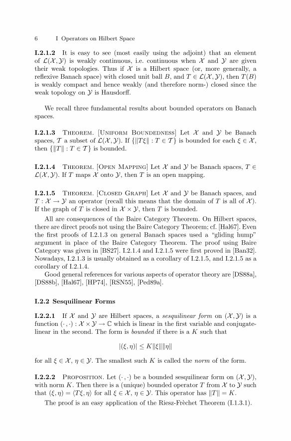
I.2.1.2 It is easy to see (most easily using the adjoint) that an elementof L(X , Y) is weakly continuous, i.e. continuous when X and Y are giventheir weak topologies. Thus if X is a Hilbert space (or, more generally, areflexive Banach space) with closed unit ball B, and T ∈ L(X , Y), then T (B)is weakly compact and hence weakly (and therefore norm-) closed since theweak topology on Y is Hausdorff.
We recall three fundamental results about bounded operators on Banachspaces.
I.2.1.3 Theorem. [Uniform Boundedness] Let X and Y be Banachspaces, T a subset of L(X , Y). If ‖Tξ‖ : T ∈ T is bounded for each ξ ∈ X ,then ‖T ‖ : T ∈ T is bounded.
I.2.1.4 Theorem. [Open Mapping] Let X and Y be Banach spaces, T ∈L(X , Y). If T maps X onto Y, then T is an open mapping.
I.2.1.5 Theorem. [Closed Graph] Let X and Y be Banach spaces, andT : X → Y an operator (recall this means that the domain of T is all of X ).If the graph of T is closed in X × Y, then T is bounded.
All are consequences of the Baire Category Theorem. On Hilbert spaces,there are direct proofs not using the Baire Category Theorem; cf. [Hal67]. Eventhe first proofs of I.2.1.3 on general Banach spaces used a “gliding hump”argument in place of the Baire Category Theorem. The proof using BaireCategory was given in [BS27]. I.2.1.4 and I.2.1.5 were first proved in [Ban32].Nowadays, I.2.1.3 is usually obtained as a corollary of I.2.1.5, and I.2.1.5 as acorollary of I.2.1.4.
Good general references for various aspects of operator theory are [DS88a],[DS88b], [Hal67], [HP74], [RSN55], [Ped89a].
I.2.2 Sesquilinear Forms
I.2.2.1 If X and Y are Hilbert spaces, a sesquilinear form on (X , Y) is afunction (· , ·) : X × Y → C which is linear in the first variable and conjugate-linear in the second. The form is bounded if there is a K such that
|(ξ, η)| ≤ K‖ξ‖‖η‖
for all ξ ∈ X , η ∈ Y. The smallest such K is called the norm of the form.
I.2.2.2 Proposition. Let (· , ·) be a bounded sesquilinear form on (X , Y),with norm K. Then there is a (unique) bounded operator T from X to Y suchthat (ξ, η) = 〈Tξ, η〉 for all ξ ∈ X , η ∈ Y. This operator has ‖T ‖ = K.
The proof is an easy application of the Riesz-Frechet Theorem (I.1.3.1).

I.2 Bounded Operators 7
I.2.2.3 Conversely, of course, any T ∈ L(X , Y) defines a bounded sesquilin-ear form (ξ, η) = 〈Tξ, η〉. There is thus a one-one correspondence betweenbounded operators and bounded sesquilinear forms. Each point of view hasits advantages. Some early authors such as Hilbert used the form approachexclusively instead of working with operators, but some parts of the theorybecome almost impossibly difficult and cumbersome (e.g. composition of op-erators) from this point of view. I. Fredholm and F. Riesz emphasized theoperator point of view, which is superior for most purposes.
I.2.2.4 The results of this subsection hold equally for operators on realHilbert spaces.
I.2.3 Adjoint
I.2.3.1 If H1 and H2 are Hilbert spaces, then each T ∈ L(H1, H2) has anadjoint , denoted T ∗, in L(H2, H1), defined by the property
〈T ∗η, ξ〉1 = 〈η, T ξ〉2
for all ξ ∈ H1, η ∈ H2, where 〈·, ·〉i is the inner product on Hi. (The existenceof T ∗ follows immediately from I.2.2.2; conversely, an operator with an adjointmust be bounded by the Closed Graph Theorem.) Adjoints have the followingproperties for all S, T ∈ L(H1, H2), α ∈ C:
(i) (S + T )∗ = S∗ + T ∗, (αT )∗ = αT ∗, and (T ∗)∗ = T ;(ii) ‖T ∗‖ = ‖T ‖ and ‖T ∗T ‖ = ‖T ‖2.
Properties (i) are obvious, and the ones in (ii) follow from the fact that‖T ‖ = sup‖ξ‖=‖η‖=1 |〈Tξ, η〉| ≥ sup‖ξ‖=1 |〈Tξ, ξ〉|.
If H = Cn, then L(H) can be naturally identified with Mn = Mn(C), and
the adjoint is the usual conjugate transpose.The range R(T ) and the null space N (T ) of a bounded operator T are sub-
spaces; N (T ) is closed, but R(T ) is not necessarily closed. The fundamentalrelationship is:
I.2.3.2 Proposition. If X and Y are Hilbert spaces and T ∈ L(X , Y), thenR(T )⊥ = N (T ∗).
I.2.3.3 An operator on a real Hilbert space has an adjoint in the same man-ner. We will primarily have occasion to consider conjugate-linear operators on(complex) Hilbert spaces. A bounded conjugate-linear operator T from H1 toH2 has a (unique) conjugate-linear adjoint T ∗ : H2 → H1 with
〈T ∗η, ξ〉1 = 〈Tξ, η〉2
for all ξ ∈ H1, η ∈ H2 (note the reversal of order in the inner product).The uniqueness of T ∗ is clear; existence can be proved by regarding T as

8 I Operators on Hilbert Space
an operator between the real Hilbert spaces H1 and H2 with inner product(ξ, η) = Re〈ξ, η〉, or directly using involutions.
An involution on a (complex) Hilbert space H is a conjugate-linear isom-etry J from H onto H with J2 = I. Involutions exist in abundance on anyHilbert space: if (ξi) is an orthonormal basis for H, then
∑αiξi → ∑
αiξi
is an involution (and every involution is of this form). If ξ, η ∈ H, then〈Jη, Jξ〉 = 〈ξ, η〉.
If T : H1 → H2 is a bounded conjugate-linear operator, and J is aninvolution on H1, then TJ is a bounded linear operator from H1 to H2;T ∗ = J(TJ)∗ is the adjoint of T (the proof uses the fact that 〈Jξ, η〉 = 〈Jη, ξ〉for all ξ, η ∈ H1, i.e. J is “self-adjoint.”)
I.2.4 Self-Adjoint, Unitary, and Normal Operators
I.2.4.1 Definition. Let H be a Hilbert space, and T ∈ L(H). Then
T is self-adjoint if T = T ∗.T is a projection if T = T ∗ = T 2.T is an isometry if T ∗T = I.T is unitary if T ∗T = TT ∗ = I.T is normal if T ∗T = TT ∗.
Self-adjoint and unitary operators are obviously normal. The usual defin-ition of an isometry is an operator T such that ‖Tξ‖ = ‖ξ‖ for all ξ. For sucha T , it follows from polarization that 〈Tξ, Tη〉 = 〈ξ, η〉 for all ξ, η, and hencethat T ∗T = I. Conversely, if T ∗T = I, then it is obvious that T is an isometryin this sense, so the definitions are equivalent. If T is an isometry, then TT ∗
is a projection. Projections will be described in I.5.If T is unitary, then T and T ∗ are isometries, and conversely; an invertible
or normal isometry is unitary.Isometries and unitary operators between different Hilbert spaces can be
defined analogously.
I.2.4.2 If T is a normal operator on H, and ξ ∈ H, then
‖Tξ‖2 = 〈Tξ, Tξ〉 = 〈T ∗Tξ, ξ〉 = 〈TT ∗ξ, ξ〉 = 〈T ∗ξ, T ∗ξ〉 = ‖T ∗ξ‖2.
(Conversely, if ‖Tξ‖ = ‖T ∗ξ‖ for all ξ, then by polarization 〈Tξ, Tη〉 =〈T ∗ξ, T ∗η〉 for all ξ, η, so T is normal.) Thus, if T is normal, N (T ) = N (T ∗) =R(T )⊥.
I.2.4.3 Examples.
(i) Let (X, µ) be a measure space, and H = L2(X, µ). For every bounded mea-surable function f : X → C there is a multiplication operator Mf ∈ L(H)defined by (Mf ξ)(x) = f(x)ξ(x) (of course, this only makes sense almost

I.2 Bounded Operators 9
everywhere). Mf is a bounded operator, and ‖Mf ‖ is the essential supre-mum of |f |. Mf Mg = Mfg for all f, g, and M∗
f = Mf , where f is thecomplex conjugate of f . Thus all Mf are normal. In fact, the SpectralTheorem implies that every normal operator looks very much like a mul-tiplication operator. Mf is self-adjoint if and only if f(x) ∈ R a.e., andMf is unitary if and only if |f(x)| = 1 a.e.
(ii) Perhaps the most important single operator is the unilateral shift S, de-fined on l2 by
S(α1, α2, . . .) = (0, α1, α2, . . .).
S is an isometry, and S∗ is the backwards shift defined by
S∗(α1, α2, . . .) = (α2, α3, . . .).
S∗S = I, but SS∗ = I (it is the projection onto the space of sequenceswith first coordinate 0). S can also be defined as multiplication by zon the Hardy space H2 of analytic functions on the unit disk with L2
boundary values on the circle T (if L2(T) is identified with l2(Z) viaFourier transform, H2 is the subspace of functions whose negative Fouriercoefficients vanish).
I.2.5 Amplifications and Commutants
I.2.5.1 If H1 and H2 are Hilbert spaces, there are natural extensions ofoperators in L(Hi) to operators on H1 ⊗ H2: if T ∈ L(H1), define T ⊗ I ∈L(H1 ⊗ H2) by
(T ⊗ I)(ξ ⊗ η) = Tξ ⊗ η.
Similarly, for S ∈ L(H2), I ⊗S is defined by (I ⊗S)(ξ⊗η) = ξ⊗Sη. T → T ⊗Iand S → I ⊗ S are isometries. The images of L(H1) and L(H2) are denotedL(H1) ⊗ I and I ⊗ L(H2) respectively, called amplifications.
I.2.5.2 More generally, if S1, T1 ∈ L(H1), S2, T2 ∈ L(H2), we can defineS1 ⊗ S2 ∈ L(H1 ⊗ H2) by
(S1 ⊗ S2)(ξ ⊗ η) = S1ξ ⊗ S2η.
ThenS1 ⊗ S2 = (S1 ⊗ I)(I ⊗ S2) = (I ⊗ S2)(S1 ⊗ I)
(S1 + T1) ⊗ S2 = (S1 ⊗ S2) + (T1 ⊗ S2)
S1 ⊗ (S2 + T2) = (S1 ⊗ S2) + (S1 ⊗ T2)
(S1 ⊗ S2)(T1 ⊗ T2) = S1T1 ⊗ S2T2
(S1 ⊗ S2)∗ = S∗1 ⊗ S∗
2
‖S1 ⊗ S2‖ = ‖S1‖‖S2‖.

10 I Operators on Hilbert Space
I.2.5.3 If S ⊆ L(H), then the commutant of S is
S ′ = T ∈ L(H) : ST = TS for all S ∈ S.
S ′ is a closed subalgebra of L(H) containing I. We denote the bicommutant(S ′)′ by S ′′. We obviously have S ⊆ S ′′, and S ′
1 ⊇ S ′2 if S1 ⊆ S2. It follows
that S ′ = (S ′′)′ for any set S.
I.2.5.4 Proposition. If H1, H2 are Hilbert spaces and H = H1 ⊗ H2, thenwe have (L(H1) ⊗ I)′ = I ⊗ L(H2) (and, similarly, (I ⊗ L(H2))′ = L(H1) ⊗ I).Thus, if S ⊆ L(H1), then (S ⊗ I)′′ = S ′′ ⊗ I.
The proof is a straightforward calculation: if ξi is an orthonormal basisfor H1, use the operators Tij ⊗ I ∈ L(H1) ⊗ I, where Tij(η) = 〈η, ξi〉ξj .
A similar calculation (cf. [KR97a, 5.5.4]) shows:
I.2.5.5 Proposition. Let H and H′ be Hilbert spaces, S1, . . . , Sn ∈ L(H),T1, . . . , Tn ∈ L(H′). Then
∑Si ⊗ Ti = 0 in L(H ⊗ H′) if and only if it is 0
in L(H) L(H′), i.e. the natural map from L(H) L(H′) to L(H ⊗ H′) isinjective.
I.2.6 Invertibility and Spectrum
In this section, we will essentially follow the first comprehensive developmentand exposition of this theory, given by F. Riesz [Rie13] in 1913, abstractedto Banach spaces and Hilbert spaces (which did not exist in 1913!) and withsome modern technical simplifications.
I.2.6.1 If T ∈ L(X , Y) (X , Y Banach spaces) is invertible in the algebraicsense, i.e. T is one-to-one and onto, then T −1 is automatically bounded bythe Open Mapping Theorem. So there are two ways a bounded operator Tcan fail to be invertible:
T is not bounded below (recall that T is bounded below if ∃ε > 0 suchthat ‖Tξ‖ ≥ ε‖ξ‖ for all ξ)R(T ) is not dense.
These possibilities are not mutually exclusive. For example, if T is a normaloperator on a Hilbert space, then N (T ) = R(T )⊥, so if R(T ) is not dense, thenT is not one-to-one and hence not bounded below. Thus a normal operatoron a Hilbert space is invertible if and only if it is bounded below.
I.2.6.2 Definition. Let X be a normed vector space, T ∈ L(X ). The spec-trum of T is
σ(T ) = λ ∈ C : T − λI is not invertible

I.2 Bounded Operators 11
The spectrum of T can be thought of as the set of “generalized eigenvalues”of T (note that every actual eigenvalue of T is in the spectrum). The firstdefinition (not the same as the one here – essentially the reciprocal) andname “spectrum” were given by Hilbert; the modern definition is due to F.Riesz.
I.2.6.3 If |λ| > ‖T ‖, then the series −λ∑∞
n=0(λ−1T )n converges absolutelyto an inverse for T − λI, so σ(T ) ⊆ λ : |λ| ≤ ‖T ‖.
It follows from general theory for (complex) Banach algebras (cf. II.1.4)that σ(T ) is nonempty and compact. Thus the spectral radius
r(T ) = max|λ| : λ ∈ σ(T )makes sense and satisfies r(T ) ≤ ‖T ‖.
I.2.6.4 The numerical range of an operator T on a Hilbert space H is
W (T ) = 〈Tξ, ξ〉 : ‖ξ‖ = 1.
Setw(T ) = sup|λ| : λ ∈ W (T ).
It is obvious that W (T ∗) = λ : λ ∈ W (T ), so w(T ∗) = w(T ); if T = T ∗,then W (T ) ⊆ R. (Conversely, if W (T ) ⊆ R, then T = T ∗: for ξ, η ∈ H, expand〈T (ξ + η), ξ + η〉 ∈ R and 〈T (ξ + iη), ξ + iη〉 ∈ R.)
I.2.6.5 Proposition. If T ∈ L(H), then σ(T ) ⊆ W (T ) and r(T ) ≤ w(T ) ≤‖T ‖.
To see that σ(T ) ⊆ W (T ), note that if λ ∈ σ(T ), then either T − λI or(T − λI)∗ is not bounded below, so there is a sequence (ξn) of unit vectorssuch that either (T − λI)ξn → 0 or (T − λI)∗ξn → 0. In either case, we obtainthat 〈(T − λI)ξn, ξn〉 → 0.
I.2.6.6 Note that r(T ) = w(T ) = ‖T ‖ does not hold for general operators:for example, let T be the (nilpotent) operator on C
2 given by the matrix[0 01 0
]
. Then σ(T ) = 0, so r(T ) = 0; but ‖T ‖ = 1. It can be shown by
an easy calculation that W (T ) = λ : |λ| ≤ 1/2, so w(T ) = 1/2. (There arealso operators on infinite-dimensional Hilbert spaces whose numerical rangeis not closed.)
I.2.6.7 Definition. A (necessarily self-adjoint) operator T on a Hilbertspace H is positive if 〈Tξ, ξ〉 ≥ 0 for all ξ. Write T ≥ 0 if T is positive, andwrite L(H)+ for the set of positive operators on H.
If T ∈ L(H), then T ∗T ≥ 0 (this is also true if T is conjugate-linear); ifT = T ∗, then λI − T ≥ 0 for λ ≥ ‖T ‖. Sums and nonnegative scalar multiplesof positive operators are positive.
If S, T are self-adjoint operators, write S ≤ T if T − S ≥ 0, i.e. if 〈Sξ, ξ〉 ≤〈Tξ, ξ〉 for all ξ.
12 I Operators on Hilbert Space
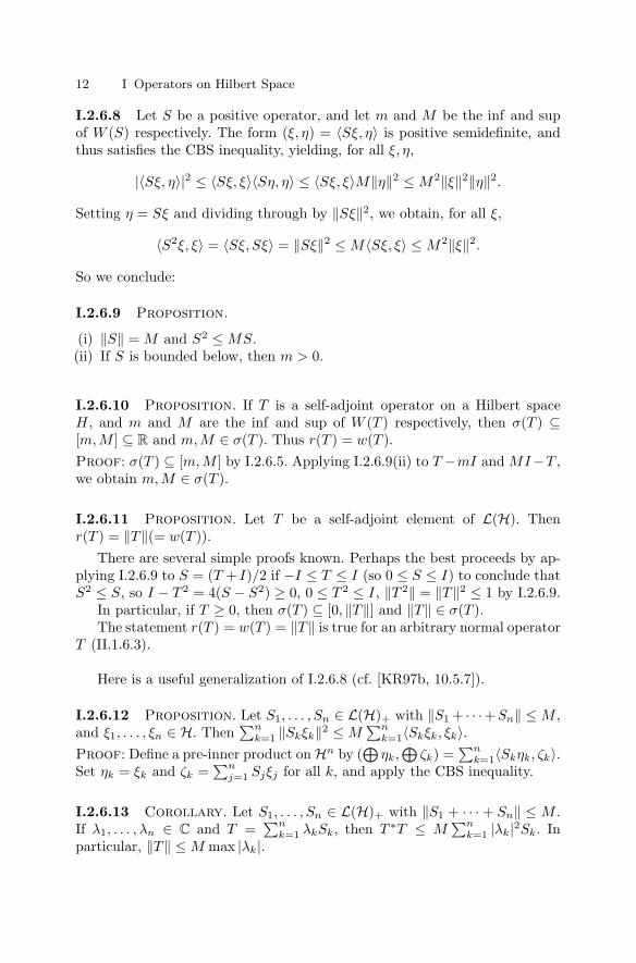
I.2.6.8 Let S be a positive operator, and let m and M be the inf and supof W (S) respectively. The form (ξ, η) = 〈Sξ, η〉 is positive semidefinite, andthus satisfies the CBS inequality, yielding, for all ξ, η,
|〈Sξ, η〉|2 ≤ 〈Sξ, ξ〉〈Sη, η〉 ≤ 〈Sξ, ξ〉M‖η‖2 ≤ M2‖ξ‖2‖η‖2.
Setting η = Sξ and dividing through by ‖Sξ‖2, we obtain, for all ξ,
〈S2ξ, ξ〉 = 〈Sξ, Sξ〉 = ‖Sξ‖2 ≤ M〈Sξ, ξ〉 ≤ M2‖ξ‖2.
So we conclude:
I.2.6.9 Proposition.
(i) ‖S‖ = M and S2 ≤ MS.(ii) If S is bounded below, then m > 0.
I.2.6.10 Proposition. If T is a self-adjoint operator on a Hilbert spaceH, and m and M are the inf and sup of W (T ) respectively, then σ(T ) ⊆[m, M ] ⊆ R and m, M ∈ σ(T ). Thus r(T ) = w(T ).Proof: σ(T ) ⊆ [m, M ] by I.2.6.5. Applying I.2.6.9(ii) to T −mI and MI −T ,we obtain m, M ∈ σ(T ).
I.2.6.11 Proposition. Let T be a self-adjoint element of L(H). Thenr(T ) = ‖T ‖(= w(T )).
There are several simple proofs known. Perhaps the best proceeds by ap-plying I.2.6.9 to S = (T + I)/2 if −I ≤ T ≤ I (so 0 ≤ S ≤ I) to conclude thatS2 ≤ S, so I − T 2 = 4(S − S2) ≥ 0, 0 ≤ T 2 ≤ I, ‖T 2‖ = ‖T ‖2 ≤ 1 by I.2.6.9.
In particular, if T ≥ 0, then σ(T ) ⊆ [0, ‖T ‖] and ‖T ‖ ∈ σ(T ).The statement r(T ) = w(T ) = ‖T ‖ is true for an arbitrary normal operator
T (II.1.6.3).
Here is a useful generalization of I.2.6.8 (cf. [KR97b, 10.5.7]).
I.2.6.12 Proposition. Let S1, . . . , Sn ∈ L(H)+ with ‖S1 + · · · + Sn‖ ≤ M ,and ξ1, . . . , ξn ∈ H. Then
∑nk=1 ‖Skξk‖2 ≤ M
∑nk=1〈Skξk, ξk〉.
Proof: Define a pre-inner product on Hn by (⊕
ηk,⊕
ζk) =∑n
k=1〈Skηk, ζk〉.Set ηk = ξk and ζk =
∑nj=1 Sjξj for all k, and apply the CBS inequality.
I.2.6.13 Corollary. Let S1, . . . , Sn ∈ L(H)+ with ‖S1 + · · · + Sn‖ ≤ M .If λ1, . . . , λn ∈ C and T =
∑nk=1 λkSk, then T ∗T ≤ M
∑nk=1 |λk|2Sk. In
particular, ‖T ‖ ≤ M max |λk|.

I.3 Other Topologies on L(H) 13
Another application of the CBS inequality gives:
I.2.6.14 Proposition. Let T be a positive operator on a Hilbert space H,and ξ, η ∈ H. Then 〈T (ξ + η), ξ + η〉 ≤ [〈Tξ, ξ〉1/2 + 〈Tη, η〉1/2]2.Proof: We have 〈T (ξ + η), ξ + η〉 = 〈Tξ, ξ〉 + 2Re〈Tξ, η〉 + 〈Tη, η〉, and bythe CBS inequality Re〈Tξ, η〉 ≤ [〈Tξ, ξ〉〈Tη, η〉]1/2.
I.2.6.15 Corollary. Let T be a positive operator on H, and ξi a totalset of vectors in H. If 〈Tξi, ξi〉 = 0 for all i, then T = 0.
An important special case is worth noting:
I.2.6.16 Corollary. Let H1 and H2 be Hilbert spaces, and T a positiveoperator on H1 ⊗ H2. If 〈T (ξ1 ⊗ ξ2), ξ1 ⊗ ξ2〉 = 0 for all ξ1 ∈ H1, ξ2 ∈ H2,then T = 0. (Actually ξ1 and ξ2 need only range over total subsets of H1 andH2 respectively.)
I.3 Other Topologies on L(H)
L(H) has several other useful topologies in addition to the norm topology.
I.3.1 Strong and Weak Topologies
I.3.1.1 Definition.The strong operator topology on L(H) is the topology of pointwise norm-con-vergence, i.e. Ti → T strongly if Tiξ → Tξ for all ξ ∈ H.The weak operator topology on L(H) is the topology of pointwise weak con-vergence, i.e. Ti → T weakly if 〈Tiξ, η〉 → 〈Tξ, η〉 for all ξ, η ∈ H.
The word “operator” is often omitted in the names of these topologies; thisusually causes no confusion, although technically there is a different topol-ogy on L(H) (more generally, on any Banach space) called the “weak topol-ogy,” the topology of pointwise convergence for linear functionals in L(H)∗.This topology, stronger than the weak operator topology, is rarely used onL(H). In this volume, “weak topology” will mean “weak operator topology,”and “strong topology” will mean “strong operator topology.” (Caution: insome references, “strong topology” or “strong convergence” refers to the normtopology.)
I.3.1.2 If (Ti) is a (norm-)bounded net in L(H), then Ti → T in the strong[resp. weak] operator topology if and only if Tiξ → Tξ in norm [resp. weakly]for a dense (or just total) set of ξ. Boundedness is essential here; a stronglyconvergent net need not be bounded. (A weakly convergent sequence must bebounded by the Uniform Boundedness Theorem.)

14 I Operators on Hilbert Space
I.3.1.3 There are variants of these topologies, called the σ-strong (or ultra-strong) operator topology and the σ-weak (or ultraweak) operator topology . A(rather unnatural) definition of these topologies is to first form the amplifi-cation H∞ = H ⊗ l2; then the restriction of the weak [resp. strong] topologyon L(H∞) to the image L(H) ⊗ I is the σ-weak [resp. σ-strong] topology onL(H). An explicit description of the topologies in terms of sets of vectors inH can be obtained from this. A more natural definition will be given in I.8.6;the σ-strong and σ-weak topologies are actually more intrinsic to the Banachspace structure of L(H) than the weak or strong topologies.
I.3.1.4 As the names suggest, the weak operator topology is weaker thanthe strong operator topology, and the σ-weak is weaker than the σ-strong. Theweak is weaker than the σ-weak, and the strong is weaker than the σ-strong.The weak and σ-weak topologies are not much different: they coincide on all(norm-)bounded sets, as follows easily from I.3.1.2. Similarly, the strong andσ-strong coincide on bounded sets. All are locally convex Hausdorff vectorspace topologies (the strong operator topology is generated by the family ofseminorms ‖ · ‖ξ, where ‖T ‖ξ = ‖Tξ‖; the others are generated by similarfamilies of seminorms.) All of these topologies are weaker than the normtopology, and none are metrizable (cf. III.2.2.28) except when H is finite-dimensional, in which case they coincide with the norm topology. (The unitball of L(H) is metrizable in both the strong and weak topologies if H isseparable.)
I.3.1.5 Examples. Let S be the unilateral shift (I.2.4.3). Then Sn → 0weakly, but not strongly. (S∗)n → 0 strongly, but not in norm.
I.3.1.6 This example shows that the adjoint operation is not strongly con-tinuous. (It is obviously weakly continuous.) One can define another, strongertopology, the strong-* operator topology , by the seminorms T → ‖Tξ‖ andT → ‖T ∗ξ‖ for ξ ∈ H, in which the adjoint is continuous. There is similarly aσ-strong-* operator topology.
Even though the adjoint is not strongly continuous, the set of self-adjointoperators is strongly closed (because it is weakly closed).
I.3.2 Properties of the Topologies
I.3.2.1 Addition and scalar multiplication are jointly continuous in all thetopologies. Multiplication is separately continuous in all the topologies, andis jointly strongly and strong-* continuous on bounded sets. However, mul-tiplication is not jointly strongly (or strong-*) continuous. Example I.3.1.5shows that multiplication is not jointly weakly continuous even on boundedsets: Sn and (S∗)n both converge to 0 weakly, but (S∗)nSn = I for all n. Theseparate weak continuity of multiplication implies that S ′ is weakly closed forany S ⊆ L(H).

I.3 Other Topologies on L(H) 15
I.3.2.2 The (closed) unit ball of L(H) is complete in all these topologies[although L(H) itself is not weakly or strongly complete if H is infinite-dimensional: if T is an unbounded everywhere-defined operator on H, foreach finite-dimensional subspace F of H let TF = T PF , where PF is theorthogonal projection onto F . Then (TF ) is a strong Cauchy net in L(H)which does not converge weakly in L(H). However, L(H) is σ-strongly andσ-strong-* complete (II.7.3.7, II.7.3.11)!] In fact, since the σ-weak operatortopology coincides with the weak-* topology on L(H) when regarded as thedual of the space of the trace-class operators (I.8.6), the unit ball of L(H)is compact in the weak operator topology. This can be proved directly usingBanach limits, which are also useful in other contexts:
I.3.2.3 Let Ω be a fixed directed set. Let Cb(Ω) be the set of all boundedfunctions from Ω to C. With pointwise operations and supremum norm, Cb(Ω)is a Banach space (in fact, it is a commutative C*-algebra). For i ∈ Ω, letπi : Cb(Ω) → C be evaluation at i; then πi is a homomorphism and a linearfunctional of norm 1 (in fact, it is a pure state (II.6.2.9)). A pure Banachlimit on Ω is a weak-* limit point ω of the net (πi) in the unit ball of Cb(Ω)∗
(which is weak-* compact). We usually write limω(λi) for ω((λi)). A pureBanach limit has the following properties:
(i) limω(λi + µi) = (limω λi) + (limω µi).(ii) limω(λµi) = λ(limω µi).
(iii) limω(λiµi) = (limω λi)(limω µi).(iv) limω λi is the complex conjugate of limω λi.(v) lim inf |λi| ≤ | limω λi| ≤ lim sup |λi|.
(vi) If λi → λ, then λ = limω λi.
A Banach limit on Ω is an element of the closed convex hull of the pureBanach limits on Ω, i.e. an element of ∩i∈Ωcoπj |j ≥ i. A Banach limit hasthe same properties except for (iii) in general.
I.3.2.4 Banach limits can also be defined in L(H). Again fix Ω and a Banachlimit ω on Ω. If (Ti) is a bounded net in L(H), for ξ, η ∈ H define (ξ, η) =limω〈Tiξ, η〉. Then (·, ·) is a bounded sesquilinear form on H, so, by I.2.2.2,there is a T ∈ L(H) with (ξ, η) = 〈Tξ, η〉 for all ξ, η. Write T = limω Ti. ThisBanach limit has the following properties:
(i) limω(Si + Ti) = (limω Si) + (limω Ti).(ii) limω(λTi) = λ(limω Ti).
(iii) ‖ limω Ti‖ ≤ lim sup ‖Ti‖.(iv) limω(T ∗
i ) = (limω Ti)∗.(v) limω Ti is a weak limit point of (Ti).
(vi) If Ti → T weakly, then T = limω Ti.
Property (v) implies the weak compactness of the unit ball of L(H).
The most useful version of completeness for the strong operator topologyis the following:

16 I Operators on Hilbert Space
I.3.2.5 Proposition. Let (Ti) be a bounded increasing net of positive op-erators on a Hilbert space H (i.e. Ti ≤ Tj for i ≤ j, and ∃K with ‖Ti‖ ≤ Kfor all i). Then there is a positive operator T on H with Ti → T strongly, and‖T ‖ = sup ‖Ti‖. T is the least upper bound for Ti in L(H)+.
For the proof, an application of the CBS inequality yields that, for anyξ ∈ H, (Tiξ) is a Cauchy net in H, which converges to a vector we call Tξ.It is easy to check that T thus defined is linear, bounded, and positive, andTi → T strongly by construction.
It follows that every decreasing net of positive operators converges stronglyto a positive operator.
I.3.2.6 Corollary. Let (Ti) be a monotone increasing (or decreasing) netof positive operators converging weakly to an operator T . Then Ti → Tstrongly, and T is the least upper bound (or greatest lower bound) of Ti.
Indeed, if (Ti) is increasing and weakly convergent to T , then 0 ≤ Ti ≤ Tfor all i, so ‖Ti‖ ≤ ‖T ‖.
Here is a simple, but useful, fact which is closely related (in fact, combinedwith I.8.6 gives an alternate proof of I.3.2.5):
I.3.2.7 Proposition. Let (Ti) be a net in L(H), and suppose T ∗i Ti → 0
weakly. Then
(i) Ti → 0 strongly.(ii) If Ti is bounded, then T ∗
i Ti → 0 strongly.
Proof: (i): If 〈T ∗i Tiξ, η〉 → 0 for all ξ, η, then for all ξ,
‖Tiξ‖2 = 〈Tiξ, Tiξ〉 = 〈T ∗i Tiξ, ξ〉 → 0.
(ii) If ‖Ti‖ ≤ K for all i, then for any ξ, ‖T ∗i Tiξ‖ ≤ K‖Tiξ‖ → 0.
I.3.2.8 Corollary. Let (Si) be a bounded net of positive operators con-verging weakly to 0. Then Si → 0 strongly.
Proof: Set Ti = S1/2i (I.4.2).
Caution: I.3.2.6 and I.3.2.8 do not mean that the strong and weak topologiescoincide on the positive part of the unit ball of L(H)!
They do, however, coincide on the set of unitaries:
I.3.2.9 Proposition. The strong, weak, σ-strong, σ-weak, strong-*, andσ-strong-* topologies coincide on the group U(H) of unitary operators on H,and make U(H) into a topological group.
The agreement of the strong and weak topologies on U(H) follows immedi-ately from I.1.3.3. The adjoint (inverse) is thus strongly continuous on U(H),

I.4 Functional Calculus 17
so the strong and strong-* topologies coincide. The σ-topologies agree withthe others on bounded sets. Multiplication is jointly strongly continuous onbounded sets.
Note, however, that the closure of U(H) in L(H) is not the same in thestrong, weak, and strong-* topologies. The strong closure of U(H) consists ofisometries (in fact, all isometries; cf. [Hal67, Problem 225]), and thus U(H)is strong-* closed; whereas the weak closure includes coisometries (adjoints ofisometries) also. Thus the unilateral shift S is in the strong closure, but notthe strong-* closure, and S∗ is in the weak closure but not the strong closure.In fact, the weak closure of U(H) is the entire closed unit ball of L(H) [Hal67,Problem 224].
I.3.2.10 Theorem. [DD63] Let H be an infinite-dimensional Hilbert space.Then U(H) is contractible in the weak/strong/strong-* topologies, and theunit sphere ξ ∈ H : ‖ξ‖ = 1 of H is contractible in the norm topology.Proof: First suppose H is separable, and hence H can be identified withL2[0, 1]. For 0 < t ≤ 1, let Vt ∈ L(H) be defined by [Vt(f)](s) = t−1/2f(s/t)(setting f(s) = 0 for s > 1). Then Vt is an isometry, V1 = I, and t → Vt andt → V ∗
t are strongly continuous. If Pt = VtV∗
t , then Pt is a projection (it is theprojection onto the subspace L2[0, t]) and t → Pt is strongly continuous. Infact, Pt is multiplication by χ[0,t]. Then, as t → 0, Vt → 0 weakly and Pt → 0strongly, and the map from U(H) × [0, 1] to U(H) defined by
(U, t) → VtUV ∗t + (I − Pt)
for t > 0 and (U, 0) → I is continuous and gives a contraction of U(H).Similarly, if f ∈ L2[0, 1], ‖f‖ = 1, set
H(f, t) = t1/2Vtf + (1 − t)1/2χ[t,1];
this gives a contraction of the unit sphere of H.For a general H, H ∼= L2[0, 1] ⊗ H. Use the same argument with Vt ⊗ I
and Pt ⊗ I in place of Vt, Pt.If H is infinite-dimensional, then N. Kuiper [Kui65] proved that U(H) is
also contractible in the norm topology. The same is true for the unitary groupof any properly infinite von Neumann algebra [BW76] and of the multiplieralgebra of a stable σ-unital C*-algebra [CH87]. Note that the result fails ifdim(H) = n < ∞: the algebraic topology of U(n, C) is fairly complicated.
I.4 Functional Calculus
We continue to follow the exposition of [Rie13] with some modernizations.There is a very important procedure for applying functions to operators
called functional calculus. Polynomials with complex coefficients can be ap-plied to any operator in an obvious way. This procedure can be extended

18 I Operators on Hilbert Space
to holomorphic functions of arbitrary operators in a way described in II.1.5.For self-adjoint operators (and, more generally, for normal operators), thisfunctional calculus can be defined for continuous functions and even boundedBorel measurable functions, as we now describe.
I.4.1 Functional Calculus for Continuous Functions
To describe the procedure for defining a continuous function of a self-adjointoperator, we first need a simple fact called the Spectral Mapping Theorem forpolynomials:
I.4.1.1 Proposition. Let T ∈ L(H), and let p be a polynomial with com-plex coefficients. Then σ(p(T )) = p(λ) : λ ∈ σ(T ).The proof is an easy application of the Fundamental Theorem of Algebra: ifλ ∈ C, write p(z) − λ = α(z − µ1) · · · (z − µn); then
p(T ) − λI = α(T − µ1I) · · · (T − µnI)
and, since the T − µkI commute, p(T ) − λI is invertible if and only if all theT − µkI are invertible.
Combining this result with I.2.6.10, we get:
I.4.1.2 Corollary. If T is self-adjoint and p is a polynomial with realcoefficients, then ‖p(T )‖ = max|p(λ)| : λ ∈ σ(T ).
(This is even true if p has complex coefficients (II.2.3.2)).
I.4.1.3 If T is self-adjoint and m, M are as in I.2.6.10, then polynomials withreal coefficients are uniformly dense in the real-valued continuous functionson [m, M ] by the Stone-Weierstrass Theorem. If f is a real-valued continu-ous function on σ(T ) and (pn) is a sequence of polynomials with real coef-ficients converging uniformly to f on σ(T ), then (pn(T )) converges in normto a self-adjoint operator we may call f(T ). The definition of f(T ) does notdepend on the choice of the sequence (pn). We have that f → f(T ) is anisometric algebra-isomorphism from the real Banach algebra CR(σ(T )), withsupremum norm, onto the closed real subalgebra of L(H) generated by T .(This homomorphism extends to complex-valued continuous functions in amanner extending the application of polynomials with complex coefficients.)Since f(T ) is a limit of polynomials in T , f(T ) ∈ T ′′; in particular, thef(T ) all commute with each other.
We have that f(T ) ≥ 0 if and only if f ≥ 0 on σ(T ); more generally, wehave σ(f(T )) ⊆ [n, N ], where
n = minf(λ) : λ ∈ σ(T ), N = maxf(λ) : λ ∈ σ(T ).
(Actually, with a bit more work (II.2.3.2) one can show the Spectral MappingTheorem in this context: σ(f(T )) = f(λ) : λ ∈ σ(T ).)

I.5 Projections 19
I.4.2 Square Roots of Positive Operators
Applying this procedure to the function f(t) = tα, we get:
I.4.2.1 Proposition. If T ≥ 0, then there is a continuous function α → T α
from R+ to L(H)+ satisfying T αT β = T α+β ∀α, β and T 1 = T . T α ∈ T ′′.In particular, if α = 1/2 we get a positive square root for T .
I.4.2.2 Corollary. Every positive operator has a positive square root.In fact, the operator T 1/2 is the unique positive square root of T
(II.3.1.2(vii)).T 1/2 can be, and often is, explicitly defined using a sequence of polynomials
converging uniformly to the function f(t) = t1/2. For example, if ‖T ‖ ≤ 1 thesequence p0 = 0, pn+1(t) = pn(t) + 1
2 (t − pn(t)2) increases to f(t) on [0, 1],and hence pn(T ) T 1/2.
I.4.2.3 If T is self-adjoint, we define T+, T−, and |T | to be f(T ), g(T ), andh(T ) respectively, where f(t) = max(t, 0), g(t) = − min(t, 0), and h(t) = |t| =f(t) + g(t). We have T+, T−, |T | ∈ T ′′, T+, T−, |T | ∈ L(H)+, T = T+ − T−,|T | = T+ + T−, T+T− = 0, |T | = (T 2)1/2. T+ and T− are called the positiveand negative parts of T , and |T | is the absolute value of T .
If T is an arbitrary element of L(H), define |T | to be (T ∗T )1/2.
I.4.3 Functional Calculus for Borel Functions
I.4.3.1 If T is self-adjoint, m, M as above, and f is a bounded nonnegativelower semicontinuous function on [m, M ], choose an increasing sequence fn ofnonnegative continuous functions on [m, M ] converging pointwise to f . Then(fn(T )) is a bounded increasing sequence of positive operators, and henceconverges strongly to a positive operator we may call f(T ). The definition off(T ) is independent of the choice of the fn, and f(T ) ∈ T ′′. Similar consid-erations apply to decreasing sequences and upper semicontinuous functions.
I.4.3.2 If f is a bounded real-valued Borel measurable function on [m, M ],then f can be obtained by taking successive pointwise limits of increasingand decreasing sequences (perhaps transfinitely many times) beginning withcontinuous functions. We may then define f(T ) in the analogous way. Thisis again well defined; f(T ) ∈ T ′′. See III.5.2.13 for a slick and rigoroustreatment of Borel functional calculus. An alternate approach to defining f(T )using the spectral theorem will be given in I.6.1.5.
I.5 Projections
Projections are the simplest non-scalar operators, and play a vital rolethroughout the theory of operators and operator algebras.

20 I Operators on Hilbert Space
I.5.1 Definitions and Basic Properties
I.5.1.1 If H is a Hilbert space and X a closed subspace, then every ξ ∈ Hcan be uniquely written as η + ζ, where η ∈ X , ζ ∈ X ⊥. The function ξ → ηis a bounded self-adjoint idempotent operator PX , called the (orthogonal)projection onto X . PX ≥ 0, P 2
X = PX , ‖PX ‖ = 1, and σ(PX ) = 0, 1.Conversely, if P ∈ L(H) satisfies P = P ∗ = P 2, then P is a projection:P = PX , where X = R(P ). There is thus a one-one correspondence betweenprojections in L(H) and closed subspaces of H.
I.5.1.2 Proposition. If X , Y are closed subspaces of H, then the followingare equivalent:
(i) PX ≤ PY (as elements of L(H)+).(ii) PX ≤ λPY for some λ > 0.
(iii) X ⊆ Y.(iv) PX PY = PYPX = PX .(v) PY − PX is a projection (it is PY∩X ⊥).
I.5.1.3 The set Proj(H) of projections in L(H) is a complete lattice (Boo-lean algebra). PX ∧ PY = PX ∩Y , PX ∨ PY = P(X +Y)− , P ⊥
X = PX ⊥ = I − PX .∧i PXi
= P∩Xiand
∨i PXi
= P(∑ Xi)− . If P and Q commute, then P ∧Q = P Q
and P ∨ Q = P + Q − P Q.If (Pi) is an increasing net of projections, then Pi → ∨
i Pi strongly; if (Pi)is decreasing, then Pi → ∧
i Pi strongly.
I.5.1.4 Remark.Note that L(H)+ is not a lattice unless H is one-dimensional.
For example, P =[
1 00 0
]
and Q = 12
[1 11 1
]
have no least upper bound
in (M2)+. [The matrices I =[
1 00 1
]
and P + Q = 12
[3 11 1
]
are upper
bounds, but there is no T with P, Q ≤ T ≤ I, P +Q, i.e. (M2)+ does not havethe Riesz Interpolation Property.] Thus the supremum of P and Q in Proj(H)is not necessarily a least upper bound of P and Q in L(H)+.
However, if (Pi) is an increasing net of projections in L(H), then P =∨
Pi
is the least upper bound for Pi in L(H)+, since Pi → P strongly, and foreach T ∈ L(H)+, S ∈ L(H) : 0 ≤ S ≤ T is strongly closed.
I.5.1.5 The lattice operations are not distributive in general: if P, Q, R areprojections in L(H), then it is not true in general that (P ∨ Q) ∧ R =(P ∧ R) ∨ (Q ∧ R) (this equality does hold if P, Q, R commute). But thereis a weaker version called the orthomodular law which does hold in general:
I.5.1.6 Proposition. Let P, Q, R be projections in L(H) with P ⊥ Q andP ≤ R. Then (P + Q) ∧ R = P ∨ (Q ∧ R).

I.5 Projections 21
I.5.1.7 As with unitaries (I.3.2.9), the strong, weak, σ-strong, σ-weak,strong-* topologies coincide on the set of projections on H, using I.1.3.3,since if Pi → P weakly, for any ξ ∈ H we have
‖Piξ‖2 = 〈Piξ, ξ〉 → 〈P ξ, ξ〉 = ‖P ξ‖2.
The set of projections is strongly closed. The weak closure is the positiveportion of the closed unit ball.
Projections in Tensor Products
Let H1 and H2 be Hilbert spaces, and P and Q projections in L(H1) andL(H2) respectively. Then P ⊗ Q is a projection in L(H1 ⊗ H2): it is theprojection onto the subspace P H1 ⊗ QH2.
I.5.1.8 Proposition. Let Pi : i ∈ I and Qj : j ∈ J be sets of projec-tions in L(H1) and L(H2) respectively. If
∨i Pi = P in L(H1) and
∨j Qj = Q
in L(H2), then∨
i,j Pi ⊗ Qj = P ⊗ Q in L(H1 ⊗ H2).Proof: The span of PiH1 : i ∈ I is dense in P H1 and the span of QjH2 :j ∈ J is dense in QH2, so the span of
(Pi ⊗ Qj)(H1 ⊗ H2) : i ∈ I, j ∈ J
is dense in P H1 ⊗ QH2 = (P ⊗ Q)(H1 ⊗ H2).
I.5.2 Support Projections and Polar Decomposition
I.5.2.1 If T ∈ L(X , Y), then the right support projection of T is the projec-tion PT onto N (T )⊥. PT is the unique projection in L(X ) with the propertythat TPT = T and PT S = 0 whenever S ∈ L(X ) and TS = 0, and is thesmallest projection P such that TP = T . Similarly, the left support projectionof T is the projection QT ∈ L(Y) onto the closure of the range of T , i.e. theright support projection of T ∗. QT satisfies QT T = T and SQT = 0 wheneverS ∈ L(Y) and ST = 0.
If T ∈ L(H) is normal, then its left and right support projections coin-cide. If T ≥ 0, then T α → P strongly as α → 0, so PT is a strong limit ofpolynomials in T and therefore PT ∈ T ′′. Also,
T (T + εI)−1 → PT
strongly as ε → 0. In general, PT = PT ∗T and QT = QT T ∗ = PT T ∗ , so(T ∗T )α → PT and (TT ∗)α → QT strongly as α → 0.
If P , Q are projections, then P ∨ Q is the support projection of P + Q;thus P ∨ Q and P ∧ Q = I − [(I − P ) ∨ (I − Q)] are in P, Q′′.

22 I Operators on Hilbert Space
I.5.2.2 The operators |T | = (T ∗T )1/2 and T map PT X one-one onto densesubspaces of PT X and QT Y respectively. Also,
‖|T |ξ‖2 = 〈|T |ξ, |T |ξ〉 = 〈T ∗Tξ, ξ〉 = 〈Tξ, Tξ〉 = ‖Tξ‖2
for any ξ. Thus the map |T |ξ → Tξ is well-defined, linear, and isometric,and extends to an isometry U from PT X onto QT Y. U may be regardedas an element of L(X , Y) by setting U = 0 on (PT X )⊥. Then U satisfiesU∗U = PT , UU∗ = QT , and T = U |T |, and is the unique element of L(X , Y)with these properties. T = U |T | is called the (left) polar decomposition of T .The operator T also has a right polar decomposition coming from the leftpolar decomposition of T ∗; in fact,
TT ∗ = U |T |2U∗ = U(T ∗T )U∗
and by iteration (TT ∗)n = U(T ∗T )nU∗ for all n, so
|T ∗| = (TT ∗)1/2 = U(T ∗T )1/2U∗ = U |T |U∗
and hence T = U |T | = |T ∗|U . The uniqueness of polar decomposition impliesthat if T ∈ L(H) with polar decomposition T = U |T |, and V ∈ L(H) isunitary, then the polar decomposition of V T is (V U)|T |.
T (T ∗T + εIX )−1/2 converges strongly to U as ε → 0. So if T ∈ L(H), thenU ∈ T, T ∗′′, and obviously |T | ∈ T, T ∗′′ also. If T ∈ L(X , Y) and T ∗Tis invertible, then U is an isometry, and U = T (T ∗T )−1/2. So if T ∈ L(H)is invertible, then U (as well as |T |) is in the norm-closed algebra generatedby T and T ∗. Similarly, if T ∈ L(X , Y) and TT ∗ is invertible, then U is acoisometry and U = (TT ∗)−1/2T . If T is invertible (or, more generally, one-one with dense range), then U is unitary.
I.5.2.3 In general, U is a partial isometry from PT X to QT X . A partialisometry is an operator U ∈ L(X , Y) such that U∗U is a projection P . Apartial isometry U is an isometry from N (U)⊥ onto R(U), and P = U∗U =PN (U)⊥ ; UU∗ is also a projection Q = PR(U). The projections P and Q arecalled the initial and final projections, or source and range projections, of U .
There is a useful generalization of the construction of U :
I.5.2.4 Proposition. Let S, T ∈ L(H) with S∗S ≤ T ∗T . Then there is aunique W ∈ L(H) with W ∗W ≤ QT (hence ‖W‖ ≤ 1), and S = WT . IfR ∈ L(H) commutes with S, T , and T ∗, then RW = WR.Proof: W is defined on R(T ) by W (Tξ) = Sξ (W is well defined since‖Sξ‖ ≤ ‖Tξ‖ for all ξ). W extends to an operator on QT H by continuity; setW = 0 on Q⊥
T H. Then W ∗W ≤ QT and S = WT . If RT = TR, RT ∗ = T ∗R,and RS = SR, then for η = Tξ ∈ R(T ) we have
WRη = WRTξ = WTRξ = SRξ = RSξ = RWT ξ = RWη

I.6 The Spectral Theorem 23
and thus RWη = WRη for η ∈ QT H. Since R(TT ∗) = (TT ∗)R, RQT = QT R,and thus R leaves (I−QT )H invariant; thus if η ∈ Q⊥
T H, then WRη = RWη =0.
A simple matrix trick yields a multivariable version:
I.5.2.5 Proposition. Let S, T1, . . . , Tn ∈ L(H) with S∗S ≤ ∑nk=1 T ∗
k Tk.Then there are unique W1, . . . , Wn ∈ L(H) with
n∑
k=1
W ∗k Wk ≤ Q∑
T ∗k Tk
(hence ‖Wk‖ ≤ 1), and S =∑n
k=1 WkTk. If R ∈ L(H) commutes with S, Tk,and T ∗
k (1 ≤ k ≤ n), then RWk = WkR (1 ≤ k ≤ n).
Proof: Identify L(Hn) with Mn(L(H)), and set S = diag(S, 0, · · · , 0), andT the matrix with first column T1, . . . , Tn and other entries 0. Apply I.5.2.4to obtain S = W T . Then W has first row W1, . . . , Wn and other entries 0.
I.5.2.6 If T is a bounded conjugate-linear operator on H, and J is an in-volution (I.2.3.3), then JT ∈ L(H), and T ∗T = (JT )∗(JT ), so |T | = |JT | iswell defined; if JT = U |JT | = U |T | is the polar decomposition of JT , thenT = V |T | is a polar decomposition for T , where V = JU is a “conjugate-linearpartial isometry,” i.e. V ∗V and V V ∗ are projections which are naturally theright and left support projections for T . This construction is independent ofthe choice of J (if K is another involution, then JK is unitary). We also haveJT = |T ∗J |U and (JTT ∗J)n = J(TT ∗)nJ for all n, so
|T ∗J | = (JTT ∗J)1/2 = J |T ∗|Jand hence T = J(JT ) = |T ∗|JU = |T ∗|V as in the linear case. Thus boundedconjugate-linear operators have a well-defined and unique polar decompositionwith analogous properties to those of linear operators.
I.6 The Spectral Theorem
The spectral theorem gives a complete description of self-adjoint (bounded)operators on a Hilbert space as generalized multiplication operators (I.2.4.3(i)).There are also versions of the theorem for normal operators and for unboundedself-adjoint operators. The version and exposition here comes essentially from[Rie13] with some modernizations.
I.6.1 Spectral Theorem for Bounded Self-Adjoint Operators
I.6.1.1 If T is a self-adjoint operator on a Hilbert space H and λ ∈ R, letE(λ,∞) = E(λ,∞)(T ) = P(T −λI)+ , the support projection of (T −λI)+ (I.4.2.3,I.5.2). The family E(λ,∞) : λ ∈ R is called the spectral resolution of T , andhas the following properties:

24 I Operators on Hilbert Space
E(λ,∞) ≥ E(µ,∞) if λ ≤ µ(E(λ,∞)) is strongly continuous from the rightIf σ(T ) ⊆ [m, M ], then E(λ,∞) = I for λ < m and E(λ,∞) = 0 for λ ≥ M .
I.6.1.2 We then define E[λ,∞) =∧
µ<λ E(µ,∞). We have that E[λ,∞) ≥E(λ,∞), and E[λ,∞) − E(λ,∞) is the projection onto the eigenspace ξ ∈ H :Tξ = λξ, so for “most” λ we have E[λ,∞) = E(λ,∞). Furthermore, for λ ≤ µ,set E[λ,µ] = E[λ,∞) − E(µ,∞), and similarly define E(λ,µ], E[λ,µ), and E(λ,µ).More generally, if B is any Borel subset of σ(T ), EB may be defined by suc-cessive infima and suprema. (See III.5.2.13 for another way to define the EB .)EB is called the spectral projection of T corresponding to B. The family EBsatisfies:
(i) EA ≤ EB if A ⊆ B(ii) EA ⊥ EB if A ∩ B = ∅
(iii) If A ∩ B = ∅, then EA∪B = EA + EB
(iv) If⋃
n Bn = B, then EB =∨
n EBn
(v) E∅ = 0, Eσ(T ) = I(vi) σ(EBT ) ⊆ B ∪ 0.
A family of projections with properties (i)-(v) is called a projection-valuedmeasure (or resolution of the identity) over σ(T ).
I.6.1.3 In addition, all EB are strong limits of polynomials in T and aretherefore in T ′′; in particular, all the spectral projections of T commutewith each other and with T , and the range of EB is invariant under T . (ii)and (vi) say that the range of EB is the “part” of H on which T “looks like”a multiplication operator (with multiplicity) by a function taking values in B.In particular, λI ≤ E[λ,µ]T ≤ µI on the range of E[λ,µ].
It follows easily that if σ(T ) ⊆ [m, M ] and λ0 = m < λ1 < · · · < λn = Mis a partition of [m, M ], then ‖T −∑n
i=1 λiE[λi−1,λi)‖ ≤ max|λi−λi−1|. Thuswe obtain:
I.6.1.4 Theorem. [Spectral Theorem] If T is a (bounded) self-adjointoperator on a Hilbert space H, and EB(T ) are its spectral projections, then
T =∫ ∞
−∞λ dEλ =
∫ ‖T ‖
−‖T ‖λ dEλ
under any reasonable interpretation of the integral (e.g. in the sense that theRiemann sum approximations to the integral converge in norm to T .)
One can also interpret functional calculus using the spectral resolution:

I.6 The Spectral Theorem 25
I.6.1.5 Theorem. Let T be a self-adjoint operator on a Hilbert space H,and f a bounded complex-valued Borel function on σ(T ). Then
f(T ) =∫ ∞
−∞f(λ) dEλ =
∫ ‖T ‖
−‖T ‖f(λ) dEλ
where the integral can be interpreted as a Riemann (or Riemann-Stieltjes)integral if f is (piecewise) continuous and a Lebesgue (Lebesgue-Stieltjes)integral otherwise.
I.6.2 Spectral Theorem for Normal Operators
I.6.2.1 There is also a version of the spectral theorem for normal operators.If N is a normal operator on H, write N = S+iT with S, T self-adjoint. Then,since S and T commute, the spectral projections for S and T all commutewith each other and with S and T ; the ranges of the spectral projectionsfor S are invariant under T , and vice versa. Thus, if A and B are Borelsubsets of σ(S) and σ(T ) respectively, we may set EA×B(N) = EA(S)EB(T ).By successive orthogonal sums, infima, and suprema, we may then define aspectral projection EC(N) for any Borel subset C of σ(N) ⊆ C. The familyEC(N) is a projection-valued measure over σ(N) (I.6.1.2), and we have:
I.6.2.2 Theorem. [Spectral Theorem for Normal Operators] LetN be a normal operator on a Hilbert space H, and EC(N) its spectralresolution. Then
N =∫
σ(N)
λ dEλ
where the integral can be interpreted as a Riemann integral over a rectanglein C (or as a Lebesgue integral over σ(N)).
I.6.2.3 Although there is no actual (scalar-valued) measure associated to aspectral resolution, there is a well-defined notion of a “set of measure zero”:a Borel set B has N -measure zero if EB(N) = 0. There is thus a notion of“N -almost everywhere.” In fact, there is a well-defined measure class corre-sponding to the spectral “measure.” No nonempty open set has zero measure.
I.6.2.4 If f is a bounded Borel function on σ(N), then we may define thefunctional calculus element f(N) by
f(N) =∫
σ(N)
f(λ) dEλ
where the integral can be interpreted as a Riemann integral if f is continuousand a Lebesgue integral in general. This functional calculus has the followingproperties:

26 I Operators on Hilbert Space
(i) If p is a polynomial of two variables with complex coefficients, and f(z) =p(z, z), then f(N) = p(N, N∗).
(ii) If fn → f uniformly on σ(N), then fn(N) → f(N) in norm.(iii) If (fn) is a uniformly bounded sequence and fn → f pointwise N -a.e. on
σ(N), then fn(N) → f(N) strongly.(iv) σ(f(N)) ⊆ f(λ) : λ ∈ σ(N)−, with equality if f is continuous.(v) ‖f(N)‖ is the “essential supremum” of |f | on σ(N):
‖f(N)‖ = infα > 0 : Eλ:|f(λ)|>α(N) = 0and if f is continuous, then ‖f(N)‖ = sup|f(λ)| : λ ∈ σ(N).
(vi) f(N) is self-adjoint if and only if f(z) ∈ R N -a.e.; f(N) is a projectionif and only if f(z) = 0 or 1 N -a.e. (i.e. if f is a characteristic function);f(N) is unitary if and only if |f(z)| = 1 N -a.e.
A consequence of the Spectral Theorem is a precise realization of anynormal operator as a multiplication operator:
I.6.2.5 Theorem. Let T be a normal operator on a separable Hilbert spaceH. Then, for 1 ≤ n ≤ ∞, there are disjoint Borel subsets Xn of σ(T ), with∪Xn = σ(T ), and finite regular Borel measures µn on Xn, such that T isunitarily equivalent to
⊕n Mz on
⊕n L2(Xn, µn, Hn), where Hn is an n-
dimensional Hilbert space and Mz is multiplication by f(z) = z. The Xn areuniquely determined up to sets of T -measure zero, and the µn are unique upto equivalence.
In connection with functional calculus, the following fact is significant. Itwas first proved by B. Fuglede [Fug50] in the case M = N , and the generalresult was obtained by C. Putnam [Put51]. The proof given here is from[Ros58].
I.6.2.6 Theorem. Let T, M, N ∈ L(H), with M, N normal. If TM = NT ,then TM∗ = N∗T .Proof: If p is any polynomial with complex coefficients, then Tp(M) =p(N)T , so for any λ ∈ C, TeiλM = eiλN T , i.e. T = e−iλN TeiλM . Thus, iff(λ) = e−iλN∗
TeiλM∗, f is an entire function from C to L(H), and we have
f(λ) = e−iλN∗e−iλN TeiλM eiλM∗
= e−i(λN∗+λN)Tei(λM+λM∗).
But λN∗ + λN and λM + λM∗ are self-adjoint for all λ, and thus f(λ) =U(λ)TV (λ), where U(λ), V (λ) are unitary. Thus ‖f(λ)‖ is constant, and there-fore f is constant by Liouville’s Theorem. So 0 = f ′(0) = −iN∗T + iTM∗.
I.6.2.7 Corollary. [Fuglede] If T, N ∈ L(H), N is normal, and T com-mutes with N , then T commutes with N∗ (alternatively, T ∗ commutes withN).

I.7 Unbounded Operators 27
I.6.2.8 Corollary. If T, N ∈ L(H), N is normal, T commutes with N ,and f is a bounded Borel function on σ(N), then T and T ∗ commute withf(N).
In particular, under the hypotheses, if N = U |N | is the polar decomposi-tion, then T (and also T ∗) commutes with Re(N), Im(N), U , and |N |.
I.7 Unbounded Operators
It is beyond the scope of this volume to give a complete treatment of un-bounded operators. However, at some points in the theory of von Neumannalgebras, it is very useful to work with unbounded operators, so we brieflydiscuss the parts of the theory relevant to our applications.
I.7.1 Densely Defined Operators
I.7.1.1 Definition. Let H be a Hilbert space. A partially defined operatoron H with domain D consists of (1) a subspace D of H and (2) a lineartransformation T : D → H. A densely defined operator on H with domain Dis a partially defined operator on H whose domain D is dense in H.
One can also consider partially defined operators on real Hilbert spaces,or conjugate-linear partially defined operators on (complex) Hilbert spaces.
A partially defined operator (or densely defined operator) may be boundedor unbounded. We will be almost exclusively concerned with densely definedoperators.
Note that the specification of the domain is a very important part of thedefinition of a partially defined operator (we usually write D(T ) for the do-main of T ). We will sometimes omit explicit specification of the domain wherethe omission should cause no confusion (as long as the need to specify the do-main is kept in mind). Thus a partially defined operator on H is technicallynot an operator on H in the sense of I.2.1.1 (sometimes called an everywheredefined operator) in general. A bounded densely defined operator on H ex-tends uniquely to a bounded (everywhere defined) operator on H, but we willdistinguish between the operator and its extension.
I.7.1.2 If S, T are partially defined operators on H, we say S = T if D(S) =D(T ) and S = T on D(S); we say S ⊆ T if D(S) ⊆ D(T ) and S = T on D(S)(T is called an extension of S). Define algebraic operations by letting S + Tbe the partially defined operator whose domain is D(S + T ) = D(S) ∩ D(T )and which is S + T on D(S + T ); ST is the partially defined operator whosedomain is
D(ST ) = ξ ∈ H : ξ ∈ D(T ), T ξ ∈ D(S)and which is ST on D(ST ). Thus a sum or product of densely defined op-erators is not necessarily densely defined. If T is a partially defined operator

28 I Operators on Hilbert Space
on H and S ∈ L(H), then S + T and ST have the same domain as T (butTS may have a different domain, and need not be densely defined if T is).If R, S ∈ L(H), then TR + TS ⊆ T (R + S), but equality does not hold ingeneral (e.g. if S = −R). We do always have (R + S)T = RT + ST .
One must be careful in defining commutation relations among partiallydefined operators: ST = TS implies D(ST ) = D(TS). This is a very strongrequirement: T does not even commute with the 0 operator in this sense unlessT is everywhere defined. A more useful notion if S is bounded is:
I.7.1.3 Definition. Let T be a partially defined operator on H, and S ∈L(H). Then S and T are permutable if ST ⊆ TS. More generally, if S ⊆ L(H),T is permutable with S if T is permutable with every S ∈ S. In this case, wesay T is affiliated with S ′, written T ∼ S ′.
If P is a projection in L(H) which is permutable with T , then P T P ⊆(TP )P = TP , but TP and P T P have the same domain, so TP = P T P . Also,
D((I − P )T ) = D(T ) = D(T − TP ) ⊆ D(T (I − P ))
and(I − P )Tξ = Tξ − P T ξ = Tξ − T P ξ = T (I − P )ξ
for ξ ∈ D(T ), so (I−P )T ⊆ T (I−P ) and therefore T (I−P ) = (I−P )T (I−P ),and hence P reduces T , i.e. both P and I − P map D(T ) into itself, T mapsP D(T ) and (I −P )D(T ) into themselves, and T = P T P +(I −P )T (I −P ) (inthe strict sense). Conversely, if P reduces T in this sense, then P is permutablewith T .
I.7.1.4 If T is a partially defined operator on H which is one-to-one onD(T ), then there is an “inverse” T −1 with domain D(T −1) = R(T ); T −1Tand TT −1 are the identity maps on D(T ) and R(T ) respectively. If S and Tare both one-one on their domains with “inverses” S−1 and T −1, then ST isone-one on its domain and its “inverse” (ST )−1 is precisely T −1S−1.
I.7.1.5 If T is a densely defined operator on H, then a core for T is asubspace D of D(T ) such that the graph Γ(T |D) is dense in the graph Γ(T )(viewed as subspaces of H ⊕ H). A core for T is obviously a dense subspaceof D(T ); note, however, that if T is unbounded and D is a dense subspace ofD(T ), then the graph of T |D is not in general dense in the graph of T , even ifT is self-adjoint (I.7.3.2), so the notion of core is more restrictive than just adense subspace of D(T ). If T is a set of densely defined operators, then a corefor T is a subspace D of D(T ) =
⋂T ∈T D(T ) which is simultaneously a core
for each T ∈ T . (If T has a core, then D(T ) is dense, but the converse is nottrue in general.) The notion of a core as a common domain for the operatorsin T is a useful one, even for a single operator, since there is often a denseproper subspace of D(T ) on which T is simpler to describe than on all of D(T )(e.g. I.7.4.7).

I.7 Unbounded Operators 29
I.7.2 Closed Operators and Adjoints
A partially defined operator is not continuous unless it is bounded. But thereis a vestige of continuity in an important class of operators:
I.7.2.1 Definition. A densely defined operator T on H is closed if its graphΓ(T ) is closed in H×H. A densely defined operator T is closable (or preclosed)if T has a closed extension, i.e. if the closure of Γ(T ) is the graph of a (denselydefined) operator (called the closure of T ).
An everywhere defined closed operator is bounded by the Closed GraphTheorem. Conversely, a bounded densely defined operator is closable, andits closure is its unique everywhere defined extension. We will only considerclosed (or sometimes closable) operators.
If T is closed and S ∈ L(H), then S + T is closed. If T is closed and one-to-one with dense range, then T −1 is also closed. If T is closed and boundedbelow on D(T ), then R(T ) is closed.
Closable operators have a nice alternate characterization in terms of ad-joints.
I.7.2.2 Definition. Let T be a densely defined operator on H. The adjointT ∗ of T is the partially defined operator defined as follows. The domain D(T ∗)is the set of η ∈ H for which there is a (necessarily unique) vector ζ ∈ H suchthat 〈ξ, ζ〉 = 〈Tξ, η〉 for all ξ ∈ D(T ) (i.e. η ∈ D(T ∗) if and only if the linearfunctional ξ → 〈Tξ, η〉 is bounded on D(T ) and thus extends to a boundedlinear functional on H.) Set T ∗η = ζ.A densely defined operator T is adjointable if D(T ∗) is dense in H.
If T is densely defined and bounded, then T ∗ is everywhere defined andbounded, and is the usual adjoint of the closure of T . If T is a densely definedoperator on H, then R(T )⊥ ⊆ D(T ∗) and is the null space of T ∗. If S, T aredensely defined operators and S ⊆ T , then T ∗ ⊆ S∗ (so if T is adjointable, sois S). If T is adjointable, then T ∗ is also adjointable and (T ∗)∗ ⊇ T .
If T is adjointable, then it is easily seen that T ∗ is closed. Thus, if T isadjointable, then it is closable ((T ∗)∗ is a closed extension). The converse isalso true:
I.7.2.3 Proposition. Let T be a densely defined operator on H. Then Tis closable if and only if T is adjointable. If T is closable, then (T ∗)∗ is theclosure of T .Proof: It suffices to show that if T is closed, then T is adjointable and(T ∗)∗ = T . Let V be the unitary operator on H ⊕ H defined by V (ξ, η) =(η, −ξ). V 2 = −I, and Γ(S∗) = [V Γ(S)]⊥ for any densely defined operator Son H, and in particular Γ(T ∗) = [V Γ(T )]⊥. So, since V is unitary,
V Γ(T ∗) = [V 2Γ(T )]⊥ = Γ(T )⊥

30 I Operators on Hilbert Space
[V Γ(T ∗)]⊥ = Γ(T )⊥⊥ = Γ(T )
since T is closed. If η ∈ D(T ∗)⊥, then (0, η) ∈ [V Γ(T ∗)]⊥ = Γ(T ), so η = 0 andD(T ∗) is dense. Furthermore, setting S = T ∗ above, Γ((T ∗)∗) = [V Γ(T ∗)]⊥ =Γ(T ), (T ∗)∗ = T .
I.7.2.4 Proposition. Let T be a closed operator on H which is one-to-onewith dense range, and let T −1 be its “inverse,” with domain R(T ) (so T −1 isclosed). Then T ∗ is one-one with dense range and (T ∗)−1 = (T −1)∗.Proof: Since N (T ∗) = R(T )⊥ and R(T ∗)⊥ = N (T ), T ∗ is one-one withdense range. Let U be the unitary in L(H × H) defined by U(ξ, η) = (η, ξ),and let V be as in the proof of I.7.2.3. U2 = I and UV = −V U . ThenΓ(T −1) = UΓ(T ), and
Γ((T −1)∗) = [V Γ(T −1)]⊥ = [V UΓ(T )]⊥ = [UV Γ(T )]⊥
= UΓ(T ∗) = Γ((T ∗)−1).
I.7.2.5 Definition. Let T be a densely defined operator on H. The spec-trum σ(T ) is the complement of the set of λ ∈ C such that T −λI is one-to-oneon D(T −λI) = D(T ) with dense range, and (T −λI)−1 is bounded (i.e. T −λIis bounded below on D(T ) with dense range).
The spectrum of an unbounded densely defined operator need not beclosed, bounded, or nonempty in general. If T is closed and T −λI is boundedbelow, then T − λI has closed range; hence if λ /∈ σ(T ), then the range ofT − λI is all of H.
I.7.2.6 The results of this section hold also for densely defined operators onreal Hilbert spaces, or conjugate-linear densely defined operators on (complex)Hilbert spaces, using the same arguments as in the bounded case (I.2.3.3).
I.7.3 Self-Adjoint Operators
I.7.3.1 Definition. Let T be a densely defined operator on H. Then T issymmetric if T ⊆ T ∗, and T is self-adjoint if T = T ∗.
A symmetric operator is closable (its closure is also symmetric) and a self-adjoint operator is closed. (Note, however, that the adjoint of a symmetricoperator is not symmetric in general.)
I.7.3.2 Examples. Let D2 be the set of f ∈ L2[0, 1] such that f is absolutelycontinuous and f ′ ∈ L2[0, 1],
D1 = f ∈ D2 : f(0) = f(1)

I.7 Unbounded Operators 31
D0 = f ∈ D2 : f(0) = f(1) = 0.
Then D0 is dense in L2[0, 1], and Dk has codimension one in Dk+1 (k = 0, 1).Let Tk be defined by Tkf = f ′ with domain Dk (k = 0, 1, 2). Then each Tk
is closed, T1 is self-adjoint, and T ∗0 = T2, so T0 is closed and symmetric, but
not self-adjoint. D0 is dense in D(T1), but Γ(T0) is not dense in Γ(T1). (D2
with its inner product inherited from its natural identification with Γ(T2) isthe first Sobolev space.)
There exist closed symmetric operators with no self-adjoint extension (e.g.the inverse Cayley transform of the unilateral shift). On the other hand, asymmetric operator can have more than one self-adjoint extension, and theycan be essentially different (e.g. different spectra).
I.7.3.3 If T is symmetric, then 〈Tξ, ξ〉 ∈ R for all ξ ∈ D(T ). Thus, if Tis symmetric and λ ∈ C \ R, then T − λI is bounded below by |Im(λ)| andhence is one-to-one and (T − λI)−1 is bounded. If T is closed and symmetric,then T − λI is closed and bounded below and hence has closed range. If T isself-adjoint, then (T −λI)∗ = T − λI is also one-to-one, so R(T −λI) is densein H and therefore equal to H since it is closed; thus (T −λI)−1 is everywheredefined and bounded. So, if T is self-adjoint, σ(T ) ⊆ R. Conversely, if T isclosed and symmetric and R(T − λI) is dense for some λ ∈ C \ R, then T isself-adjoint.
The next proposition is an immediate corollary of I.7.2.4.
I.7.3.4 Proposition. Let T be a self-adjoint densely defined operator onH which is one-one on D(T ) with dense range. Then the “inverse” T −1, withdomain R(T ), is self-adjoint.
I.7.3.5 Theorem. Let T be a closed operator on H. Then T ∗T is denselydefined and self-adjoint; I + T ∗T maps D(T ∗T ) one-to-one onto H, and(I + T ∗T )−1 and T (I + T ∗T )−1 are everywhere defined, bounded, and ofnorm ≤ 1, and (I + T ∗T )−1 ≥ 0. Also, D(T ∗T ) = R((I + T ∗T )−1).Proof: Let V ∈ L(H × H) be as in the proof of I.7.2.3. Then Γ(T ) =[V Γ(T ∗)]⊥, so if ζ ∈ H there are unique ξ ∈ D(T ) and η ∈ D(T ∗) suchthat (ζ, 0) = (ξ, T ξ) + (T ∗η, −η), i.e. ζ = ξ + T ∗η, 0 = Tξ − η (so η = Tξ),and
‖ξ‖2 + ‖η‖2 ≤ ‖ξ‖2 + ‖Tξ‖2 + ‖T ∗η‖2 + ‖η‖2 = ‖ζ‖2.
Set Rζ = ξ and Sζ = η. Then R and S are everywhere defined and bounded,with ‖R‖, ‖S‖ ≤ 1, and R + T ∗S = I and TR − S = 0, so S = TR and
(I + T ∗T )R = I.
In particular, TR, T ∗S = T ∗TR, and (I + T ∗T )R are everywhere defined, i.e.R(R) ⊆ D(T ∗T ). If ξ ∈ H, then
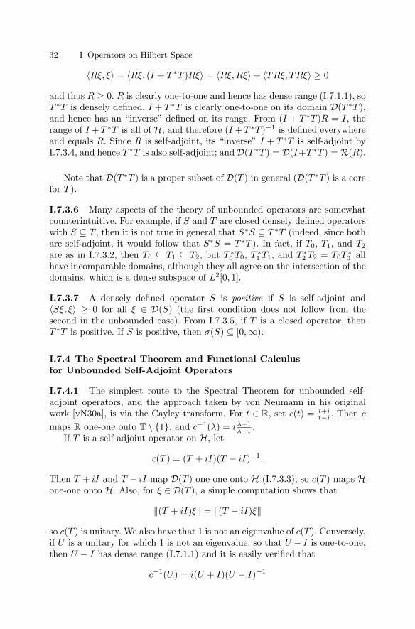
32 I Operators on Hilbert Space
〈Rξ, ξ〉 = 〈Rξ, (I + T ∗T )Rξ〉 = 〈Rξ, Rξ〉 + 〈TRξ, TRξ〉 ≥ 0
and thus R ≥ 0. R is clearly one-to-one and hence has dense range (I.7.1.1), soT ∗T is densely defined. I + T ∗T is clearly one-to-one on its domain D(T ∗T ),and hence has an “inverse” defined on its range. From (I + T ∗T )R = I, therange of I + T ∗T is all of H, and therefore (I + T ∗T )−1 is defined everywhereand equals R. Since R is self-adjoint, its “inverse” I + T ∗T is self-adjoint byI.7.3.4, and hence T ∗T is also self-adjoint; and D(T ∗T ) = D(I+T ∗T ) = R(R).
Note that D(T ∗T ) is a proper subset of D(T ) in general (D(T ∗T ) is a corefor T ).
I.7.3.6 Many aspects of the theory of unbounded operators are somewhatcounterintuitive. For example, if S and T are closed densely defined operatorswith S ⊆ T , then it is not true in general that S∗S ⊆ T ∗T (indeed, since bothare self-adjoint, it would follow that S∗S = T ∗T ). In fact, if T0, T1, and T2
are as in I.7.3.2, then T0 ⊆ T1 ⊆ T2, but T ∗0 T0, T ∗
1 T1, and T ∗2 T2 = T0T ∗
0 allhave incomparable domains, although they all agree on the intersection of thedomains, which is a dense subspace of L2[0, 1].
I.7.3.7 A densely defined operator S is positive if S is self-adjoint and〈Sξ, ξ〉 ≥ 0 for all ξ ∈ D(S) (the first condition does not follow from thesecond in the unbounded case). From I.7.3.5, if T is a closed operator, thenT ∗T is positive. If S is positive, then σ(S) ⊆ [0, ∞).
I.7.4 The Spectral Theorem and Functional Calculusfor Unbounded Self-Adjoint Operators
I.7.4.1 The simplest route to the Spectral Theorem for unbounded self-adjoint operators, and the approach taken by von Neumann in his originalwork [vN30a], is via the Cayley transform. For t ∈ R, set c(t) = t+i
t−i . Then c
maps R one-one onto T \ 1, and c−1(λ) = i λ+1λ−1 .
If T is a self-adjoint operator on H, let
c(T ) = (T + iI)(T − iI)−1.
Then T + iI and T − iI map D(T ) one-one onto H (I.7.3.3), so c(T ) maps Hone-one onto H. Also, for ξ ∈ D(T ), a simple computation shows that
‖(T + iI)ξ‖ = ‖(T − iI)ξ‖
so c(T ) is unitary. We also have that 1 is not an eigenvalue of c(T ). Conversely,if U is a unitary for which 1 is not an eigenvalue, so that U − I is one-to-one,then U − I has dense range (I.7.1.1) and it is easily verified that
c−1(U) = i(U + I)(U − I)−1
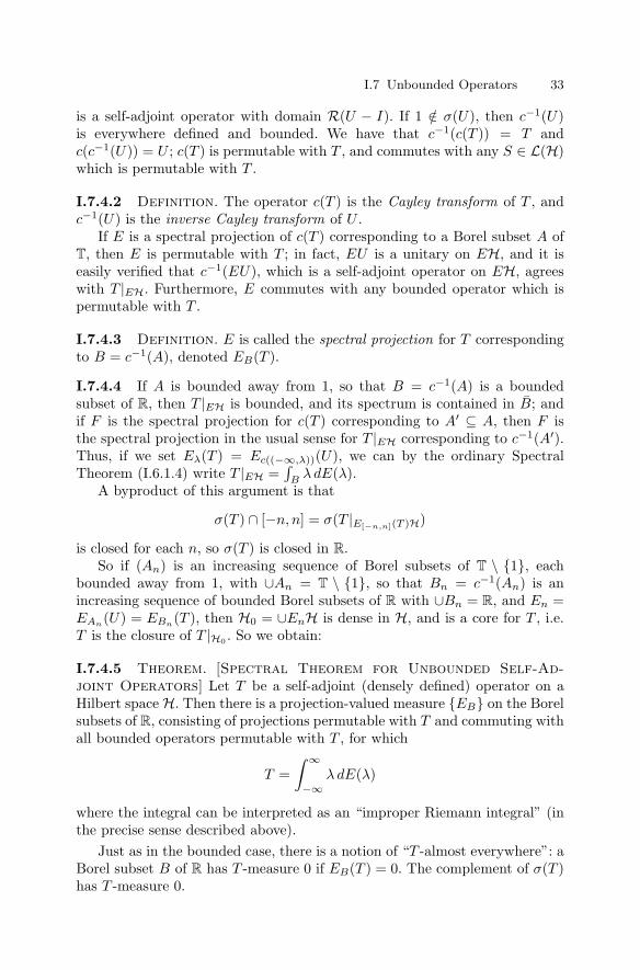
I.7 Unbounded Operators 33
is a self-adjoint operator with domain R(U − I). If 1 /∈ σ(U), then c−1(U)is everywhere defined and bounded. We have that c−1(c(T )) = T andc(c−1(U)) = U ; c(T ) is permutable with T , and commutes with any S ∈ L(H)which is permutable with T .
I.7.4.2 Definition. The operator c(T ) is the Cayley transform of T , andc−1(U) is the inverse Cayley transform of U .
If E is a spectral projection of c(T ) corresponding to a Borel subset A ofT, then E is permutable with T ; in fact, EU is a unitary on EH, and it iseasily verified that c−1(EU), which is a self-adjoint operator on EH, agreeswith T |EH. Furthermore, E commutes with any bounded operator which ispermutable with T .
I.7.4.3 Definition. E is called the spectral projection for T correspondingto B = c−1(A), denoted EB(T ).
I.7.4.4 If A is bounded away from 1, so that B = c−1(A) is a boundedsubset of R, then T |EH is bounded, and its spectrum is contained in B; andif F is the spectral projection for c(T ) corresponding to A′ ⊆ A, then F isthe spectral projection in the usual sense for T |EH corresponding to c−1(A′).Thus, if we set Eλ(T ) = Ec((−∞,λ))(U), we can by the ordinary SpectralTheorem (I.6.1.4) write T |EH =
∫B
λ dE(λ).A byproduct of this argument is that
σ(T ) ∩ [−n, n] = σ(T |E[−n,n](T )H)
is closed for each n, so σ(T ) is closed in R.So if (An) is an increasing sequence of Borel subsets of T \ 1, each
bounded away from 1, with ∪An = T \ 1, so that Bn = c−1(An) is anincreasing sequence of bounded Borel subsets of R with ∪Bn = R, and En =EAn
(U) = EBn(T ), then H0 = ∪EnH is dense in H, and is a core for T , i.e.
T is the closure of T |H0 . So we obtain:
I.7.4.5 Theorem. [Spectral Theorem for Unbounded Self-Ad-joint Operators] Let T be a self-adjoint (densely defined) operator on aHilbert space H. Then there is a projection-valued measure EB on the Borelsubsets of R, consisting of projections permutable with T and commuting withall bounded operators permutable with T , for which
T =∫ ∞
−∞λ dE(λ)
where the integral can be interpreted as an “improper Riemann integral” (inthe precise sense described above).
Just as in the bounded case, there is a notion of “T -almost everywhere”: aBorel subset B of R has T -measure 0 if EB(T ) = 0. The complement of σ(T )has T -measure 0.
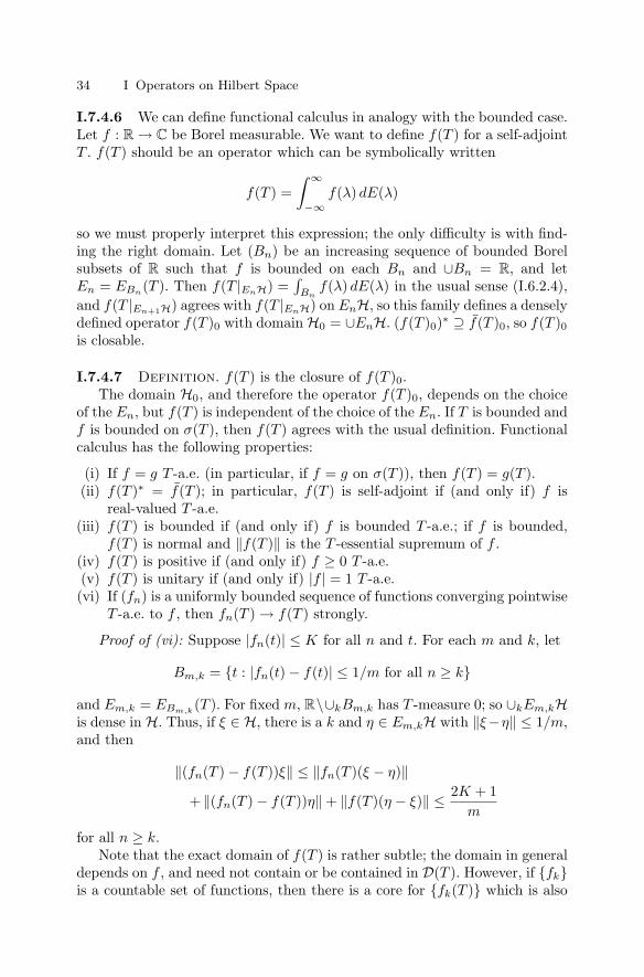
34 I Operators on Hilbert Space
I.7.4.6 We can define functional calculus in analogy with the bounded case.Let f : R → C be Borel measurable. We want to define f(T ) for a self-adjointT . f(T ) should be an operator which can be symbolically written
f(T ) =∫ ∞
−∞f(λ) dE(λ)
so we must properly interpret this expression; the only difficulty is with find-ing the right domain. Let (Bn) be an increasing sequence of bounded Borelsubsets of R such that f is bounded on each Bn and ∪Bn = R, and letEn = EBn
(T ). Then f(T |EnH) =∫
Bnf(λ) dE(λ) in the usual sense (I.6.2.4),
and f(T |En+1H) agrees with f(T |EnH) on EnH, so this family defines a denselydefined operator f(T )0 with domain H0 = ∪EnH. (f(T )0)∗ ⊇ f(T )0, so f(T )0
is closable.
I.7.4.7 Definition. f(T ) is the closure of f(T )0.The domain H0, and therefore the operator f(T )0, depends on the choice
of the En, but f(T ) is independent of the choice of the En. If T is bounded andf is bounded on σ(T ), then f(T ) agrees with the usual definition. Functionalcalculus has the following properties:
(i) If f = g T -a.e. (in particular, if f = g on σ(T )), then f(T ) = g(T ).(ii) f(T )∗ = f(T ); in particular, f(T ) is self-adjoint if (and only if) f is
real-valued T -a.e.(iii) f(T ) is bounded if (and only if) f is bounded T -a.e.; if f is bounded,
f(T ) is normal and ‖f(T )‖ is the T -essential supremum of f .(iv) f(T ) is positive if (and only if) f ≥ 0 T -a.e.(v) f(T ) is unitary if (and only if) |f | = 1 T -a.e.
(vi) If (fn) is a uniformly bounded sequence of functions converging pointwiseT -a.e. to f , then fn(T ) → f(T ) strongly.
Proof of (vi): Suppose |fn(t)| ≤ K for all n and t. For each m and k, let
Bm,k = t : |fn(t) − f(t)| ≤ 1/m for all n ≥ k
and Em,k = EBm,k(T ). For fixed m, R\∪kBm,k has T -measure 0; so ∪kEm,kH
is dense in H. Thus, if ξ ∈ H, there is a k and η ∈ Em,kH with ‖ξ −η‖ ≤ 1/m,and then
‖(fn(T ) − f(T ))ξ‖ ≤ ‖fn(T )(ξ − η)‖+ ‖(fn(T ) − f(T ))η‖ + ‖f(T )(η − ξ)‖ ≤ 2K + 1
m
for all n ≥ k.Note that the exact domain of f(T ) is rather subtle; the domain in general
depends on f , and need not contain or be contained in D(T ). However, if fkis a countable set of functions, then there is a core for fk(T ) which is also

I.7 Unbounded Operators 35
a core for T , namely ∪EBn(T )H, where (Bn) is an increasing sequence of
bounded Borel sets on which each of the fk are individually bounded, andsuch that R \ ∪Bn has T -measure 0.
This functional calculus procedure also works, and is interesting, for un-bounded Borel functions of bounded self-adjoint operators, and can be ex-tended to unbounded functions of bounded normal operators.
I.7.4.8 An important special case of functional calculus is to define T+,T−, and |T | for a self-adjoint operator T . These are positive operators. Inaddition, if T is positive, then T α can be defined for any α > 0, and inparticular for α = 1/2. Thus every positive operator has a square root. Wehave that |T | = (T 2)1/2 for any self-adjoint T .
I.7.4.9 If T is a closed operator, then there is a partial isometry V from[R(T ∗)]− to [R(T )]− such that T = V |T | = |T ∗|V . (In particular, D(|T |) =D(T ).) The proof consists of taking a dense subspace H0 of H as above, usingspectral projections for T ∗T , and then noting that ‖|T |ξ‖ = ‖Tξ‖ for ξ ∈ H0
just as in the bounded case. Thus there is polar decomposition for closedoperators. As in I.5.2.6, polar decomposition also works for closed conjugate-linear operators.
Note that if S and T are closed operators with S ⊆ T , then
D(|S|) = D(S) ⊆ D(T ) = D(|T |)
but usually |S| ⊆ |T | (I.7.3.6). For example, if T0, T1 are as in I.7.3.2, then|T0| has dense range since T0 is one-to-one, but |T1| does not have dense range.
Finally, there is a more nontrivial application of functional calculus whichis very important. Let H be a self-adjoint operator on H, and for t ∈ R
set Ut = eitH . Then Ut is unitary, Us+t = UsUt, and t → Ut is stronglycontinuous ((Ut) is a strongly continuous one-parameter group of unitaries).The map t → Ut is norm-continuous if and only if H is bounded. The converseis also true [Sto32]:
I.7.4.10 Theorem. [Stone] Let (Ut) be a strongly continuous one-para-meter group of unitaries on H. Then there is a unique self-adjoint operatorH on H, called the generator of the group, such that Ut = eitH for all t. Thedomain of H consists of all vectors ξ for which limt→0 t−1(Ut − I)ξ exists, andHξ is this limit.
In fact, if (αt) is a strongly continuous one-parameter automorphism groupof L(H), then there is such a group of unitaries such that αt = ad Ut, i.e.there is a unique (up to adding a scalar) self-adjoint operator H such thatαt(T ) = eitHTe−itH for all t ∈ R and T ∈ L(H).

36 I Operators on Hilbert Space
I.8 Compact Operators
Some of the simplest, yet most important, classes of operators are the compactoperators (often called completely continuous operators, particularly in earlierreferences), and the subclasses of finite-rank, trace-class, and Hilbert-Schmidtoperators.
I.8.1 Definitions and Basic Properties
I.8.1.1 Definition. Let X and Y be Banach spaces. An operator T : X →Y is compact if T sends bounded subsets of X to precompact subsets of Y.
In other words, if B is a bounded subset of X , then T (B) is a compactsubset of Y. Equivalently, whenever (ξn) is a bounded sequence of vectors inX , then (Tξn) has a convergent subsequence.
I.8.1.2 It is obvious that a compact operator is bounded, and the compo-sition (in either order) of a compact operator with a bounded operator iscompact. It is easily seen that a norm-limit of compact operators is compact.The set of compact operators from X to Y, denoted K(X , Y), is a closedsubspace of L(X , Y); K(H) = K(H, H) is a closed two-sided ideal in L(H).
If X is a Hilbert space (or, more generally, a reflexive Banach space),T ∈ K(X , Y), and B is the closed unit ball of X , then it follows from I.1.3.2and I.2.1.2 that T (B) is already closed and therefore compact.
I.8.1.3 Examples.
(i) Any finite-rank bounded operator is compact. Conversely, if T ∈ L(X , Y)is compact and bounded below, then X is finite-dimensional.
(ii) Let X and Y be measure spaces, and k ∈ L2(X × Y ). Define an operatorT : L2(X) → L2(Y ) by (Tf)(y) =
∫X
k(x, y)f(x) dx. T is a compactoperator, called the integral kernel operator with kernel k. (In fact, T isa Hilbert-Schmidt operator (I.8.5)).
A straightforward exercise shows:
I.8.1.4 Proposition. Let X , Y, Z be Banach spaces, T ∈ L(X , Y) compact,and (Si) a uniformly bounded net of elements of L(Y, Z) converging stronglyto S. Then SiT → ST in norm.
I.8.1.5 If Y is a Hilbert space and ηi : i ∈ Ω an orthonormal basis, for afinite subset F ⊆ Ω let PF be the projection onto the span of ηi : i ∈ F .Then PF is a finite-rank projection, and PF → I strongly. So if T ∈ L(X , Y)is compact, then PF T → T in norm, i.e. T is a norm-limit of finite-rankoperators. [This can fail if Y is not a Hilbert space [Enf73].] Thus K(X , Y) isprecisely the norm-closure of the set C(X , Y) of bounded finite-rank operators.
As a corollary, the adjoint of a compact operator is compact. If T is com-pact, T ∗T is too and so is f(T ∗T ) for any continuous function f vanishing at0. In particular, |T | = (T ∗T )1/2 is compact.

I.8 Compact Operators 37
I.8.2 The Calkin Algebra
I.8.2.1 Since K(H) is a closed ideal in L(H) for a Hilbert space H (assumedinfinite-dimensional), we may form the quotient Banach algebra Q(H) =L(H)/K(H), called the Calkin algebra of H. The term “Calkin algebra” with-out further qualification will mean the Calkin algebra of a separable, infinite-dimensional Hilbert space. We usually denote the quotient map from L(H) toQ(H) by π.
Since K(H) is self-adjoint, the involution T → T ∗ on L(H) drops to awell-defined involution on Q(H). Actually, Q(H) is a C*-algebra (II.5.1.1).
Thus all the properties and constructions for general Banach algebras, orC*-algebras, are valid for Q(H); see Chapter 2. In this chapter we will need touse only the elementary fact that the group of invertible elements in a unitalBanach algebra is open and contains the open ball of radius 1 around theidentity (II.1.3).
I.8.2.2 If T ∈ L(H), we define the essential spectrum σe(T ) to be the spec-trum of π(T ) in Q(H), i.e.
σe(T ) = λ ∈ C : π(T − λI) is not invertible in Q(H)
Clearly σe(T ) ⊆ σ(T ), and in fact σe(T ) ⊆ ∩K∈K(H)σ(T + K) (the inclusionis proper in general). By II.1.4.2, σe(T ) is a nonempty compact subset of C.
I.8.3 Fredholm Theory
The theory of Fredholm operators and Fredholm index is not only importantfor applications, but (in retrospect) was a pioneering example of bringingalgebraic topology into the theory of operator algebras (cf. II.8.4.32, II.8.4.36).In fact, it was one of the first examples of the process called “noncommutativetopology,” which underlies much of the modern theory of operator algebras.
I.8.3.1 Definition. Let X and Y be Banach spaces and T ∈ L(X , Y). ThenT is a Fredholm operator if N (T ) is finite-dimensional and R(T ) has finitecodimension. The index of T is dim N (T ) − codim R(T ).
I.8.3.2 It follows easily from the Open Mapping Theorem that the rangeof a Fredholm operator is automatically closed. Thus, if X and Y are Hilbertspaces (the only situation we will consider), then T ∈ L(X , Y) is Fredholmif and only if R(T ) is closed and N (T ) and N (T ∗) are finite-dimensional,and then index(T ) = dim N (T ) − dim N (T ∗). If T is Fredholm, thenT is bounded below on N (T )⊥; it follows that T ∗ is also Fredholm, andindex(T ∗) = −index(T ).

38 I Operators on Hilbert Space
I.8.3.3 Examples.
(i) If X and Y are finite-dimensional, then every operator from X to Y isFredholm with index dim X − dim Y.
(ii) If T is invertible, then T is Fredholm with index 0.(iii) Let S be the unilateral shift (I.2.4.3). Then S is Fredholm with index
−1. Sn is Fredholm with index −n, and (S∗)n is Fredholm with index n.
The parts of the following proposition are easy consequences of the defin-ition of a compact operator.
I.8.3.4 Proposition. Let H be a Hilbert space, T ∈ K(H), and λ ∈ C,λ = 0. Then
(i) N (T − λI) is finite-dimensional.(ii) T − λI is bounded below on N (T − λI)⊥, and hence R(T − λI) is closed.
(iii) There is an n such that N ((T − λI)n) = N ((T − λI)n+1) [T − λI hasfinite ascent .] The smallest such n is called the ascent of T − λI.
Applying the proposition to both T − λI and T ∗ − λI = (T − λI)∗, we seethat
I.8.3.5 Corollary. Let H be a Hilbert space, T ∈ K(H), and λ ∈ C,λ = 0. Then
(i) T − λI is Fredholm.(ii) There is an m such that R((T − λI)m) = R((T − λI)m+1) [T − λI has
finite descent .]
The next theorem [Atk53] gives a useful alternate characterization of Fred-holm operators.
I.8.3.6 Theorem. [Atkinson] Let H be an infinite-dimensional Hilbertspace and π : L(H) → Q(H) = L(H)/K(H) the quotient map onto the Calkinalgebra of H. Then T ∈ L(H) is Fredholm if and only if π(T ) is invertible inQ(H).Proof: If T is Fredholm, then T is bounded below on N (T )⊥, so there is anS ∈ L(H) mapping R(T ) to N (T )⊥ and zero on R(T )⊥ = N (T ∗), such thatST = I − PN (T ) and TS = I − PN (T ∗) (S is called a quasi-inverse for T ; wehave TST = T and STS = S). Thus π(S) is an inverse for π(T ).
Conversely, suppose π(T ) is invertible in Q(H), and let S ∈ L(H) suchthat π(S) = π(T )−1. Then ST = I + K, TS = I + L for K, L ∈ K(H).N (T ) ⊆ N (ST ) which is finite-dimensional by I.8.3.5; R(T ) ⊇ R(TS) hasfinite codimension by I.8.3.2.

I.8 Compact Operators 39
I.8.3.7 Corollary.
(i) If S and T are Fredholm and K ∈ K(H), then ST and T +K are Fredholm.(ii) The set F(H) of Fredholm operators on H is open.
The most important basic facts about the index function are:
I.8.3.8 Theorem. Let H be a Hilbert space.
(i) If S, T ∈ F(H), then index(ST ) = index(S) + index(T ).(ii) The index is locally constant on F(H), and hence constant on connected
components (path components) of F(H).(iii) If T ∈ F(H) and K ∈ K(H), then index(T + K) = index(T ).
The proof of (i) is a straightforward but moderately involved calculation,and (ii) is a simple consequence of (i) and the fact that the invertible operatorsform an open set. For (iii), note that T and T + K are connected by the pathT + tK : 0 ≤ t ≤ 1 in F(H).
If T is a Fredholm operator of index 0 and K is a one-one map of N (T )onto R(T )⊥, then S = T − K is invertible. Thus we obtain:
I.8.3.9 Corollary. A Fredholm operator T has index 0 if and only ifT = S + K, where S is invertible and K ∈ K(H). (So, since K(H) and theset of invertible elements in L(H) are connected, index maps the connectedcomponents of F(H) one-one onto Z.) In particular, if T ∈ K(H) and λ ∈ C,λ = 0, then T − λI has index 0.
This last result is often stated in the following form, called the FredholmAlternative:
I.8.3.10 Corollary. If T ∈ K(H) and λ ∈ C, λ = 0, then T − λI isinjective if and only if it is surjective. So if λ ∈ σ(T ), λ = 0, then λ is aneigenvalue of T .
So, under the hypotheses of the corollary, either the equation (T −λI)ξ = ηhas a unique solution for every η, or the homogeneous equation (T −λI)ξ = 0has a nontrivial (but finite-dimensional) space of solutions. This result, appliedto integral kernel operators, is important in the theory of differential andintegral equations.
I.8.3.11 If T ∈ K(H) and λ = 0, and n > 0 is the ascent of T − λI(I.8.3.4(iii)), let H0 = N ((T − λI)n), H1 = R((T − λI)n). Then H0 and H1
are complementary closed subspaces of H invariant under T −λI, (T −λI)|H0
is nilpotent, and (T −λI)|H1 is invertible. It follows that λ is an isolated pointof σ(T ). Thus σ(T ) consists of 0 and a (possibly finite) sequence of eigenvaluesconverging to 0.

40 I Operators on Hilbert Space
I.8.3.12 If T ∈ L(H), then the essential spectrum σe(T ) (I.8.2.2) is
σe(T ) = λ ∈ C : T − λI is not Fredholm.
It is not difficult to see that
∩K∈K(H)σ(T + K) = λ ∈ C : T − λI is not Fredholm of index 0.
The index is constant on connected components of C \ σe(T ) and vanishes onC \ σ(T ) and, in particular, on the unbounded component of C \ σe(T ). Thus,if C \ σe(T ) is connected, we have σe(T ) = ∩K∈K(H)σ(T + K).
I.8.3.13 Let G be the group of invertible elements of Q(H), and Go theconnected component (path component) of the identity in G. I.8.3.8 impliesthat index is a homomorphism from G/Go to the additive group Z. This mapis a special case of the connecting map in the six-term exact sequence ofK-theory (V.1.2.22) associated with the extension
0 → K(H) → L(H) → Q(H) → 0
and I.8.3.8 and I.8.3.9 imply that index is actually an isomorphism fromG/Go
∼= K1(Q(H)) onto Z ∼= K0(K(H)).
I.8.3.14 Many of the properties of Fredholm operators carry over to semi-Fredholm operators. A bounded operator T on H is semi-Fredholm if T hasclosed range and either N (T ) or N (T ∗) is finite-dimensional. The index of a(non-Fredholm) semi-Fredholm operator is well defined as ±∞, and the indexis additive where well defined (note, however, that the product of a semi-Fredholm operator of index +∞ and a semi-Fredholm operator of index −∞is not semi-Fredholm in general.) A compact perturbation of a semi-Fredholmoperator is semi-Fredholm of the same index. A version of Atkinson’s theoremholds: an operator is semi-Fredholm if and only if its image in the Calkinalgebra is left or right invertible.
I.8.3.15 Many of the results above, suitably restated, apply to Fredholmoperators between different spaces.
I.8.4 Spectral Properties of Compact Operators
Compact operators behave almost like finite-rank operators with regard tospectral theory. The spectral theory of compact operators in its modern formwas developed by F. Riesz, following important contributions of Fredholm andHilbert.
I.8.4.1 By I.8.3.4, if T ∈ K(H), each nonzero point of σ(T ) is an eigenvalueof T , the corresponding eigenspace is finite-dimensional, and the eigenvaluesform a finite set or a sequence converging to 0. (If T ∈ K(H)+, this also followsfrom the Spectral Theorem: for each λ > 0 the spectral projection E(λ,∞)(T )has finite rank, since T is bounded below on its range.)

I.8 Compact Operators 41
I.8.4.2 If T ∈ K(H), the nonzero eigenvalues of |T |, counted with multiplic-ity, can thus be arranged in a decreasing sequence
(µ0(T ), µ1(T ), · · · )
called the characteristic list (or list of characteristic numbers) for T . (Thecharacteristic list is finite if and only if T is finite-rank, in which case it isexpanded into an infinite sequence by adding zeroes.) The characteristic listsfor T and T ∗ are the same. By I.2.6.10, µ0(T ) = ‖T ‖. The characteristic listis sometimes called the eigenvalue list of T , especially if T ≥ 0.
The n’th characteristic number µn(T ) can alternately be characterized asthe distance from T to the (closed) set Cn(H) of operators in L(H) of rank≤ n (cf. [GKn69]). From this we get several useful properties such as
|µn(S) − µn(T )| ≤ ‖S − T ‖
µn+m(S + T ) ≤ µn(S) + µm(T )
µn+m(ST ) ≤ µn(S)µmT.
Denote the partial sum∑N−1
n=0 µn(T ) by σN (T ).
I.8.5 Trace-Class and Hilbert-Schmidt Operators
The trace of a finite-rank operator on a vector space is an important invariantin many contexts. The notion of trace can be extended to certain infinite-rank operators on Hilbert spaces, and this trace plays a crucial role in manyapplications, often acting as a “noncommutative integral.”
I.8.5.1 Let H be a Hilbert space and 0 ≤ T ∈ L(H). We define the traceTr(T ) to be
∑i〈Tξi, ξi〉 ∈ [0, ∞], where ξi is an orthonormal basis for H.
If S ∈ L(H), then a simple calculation shows that Tr(SS∗) = Tr(S∗S);so Tr(T ) is well defined independently of the choice of the orthonormalbasis and satisfies Tr(T ) = Tr(U∗TU) for any unitary U . Also, obviouslyTr(T ) ≥ ‖T ‖, Tr(S + T ) = Tr(S) + Tr(T ) if S, T ≥ 0, and Tr(S) ≤ Tr(T )if 0 ≤ S ≤ T . We have that Tr(T ) < ∞ if and only if T is compact and itscharacteristic list (µ0(T ), µ1(T ), · · · ) satisfies
∑n µn(T ) < ∞, in which case
Tr(T ) =∑
n µn(T ).
I.8.5.2 Tr is lower semicontinuous on L(H)+. In fact, if (Tj) is a net inL(H)+ converging weakly to T , then 〈Tjξi, ξi〉 → 〈Tξi, ξi〉 for each i, soTr(T ) ≤ lim infj Tr(Tj). (Tr is not continuous if H is infinite-dimensional,however: if Pn is a rank n projection and Tn = 1
n Pn, then Tn → 0 butTr(Tn) = 1 for all n.)
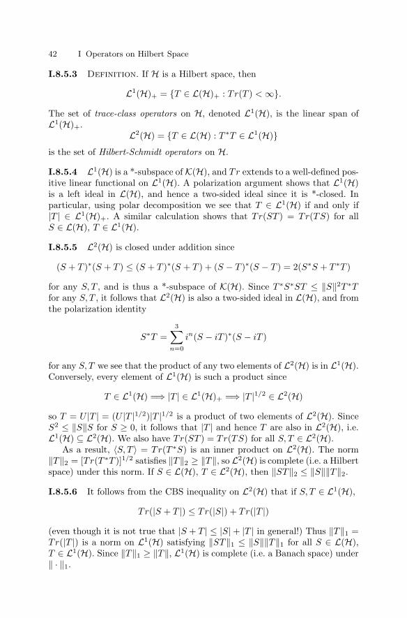
42 I Operators on Hilbert Space
I.8.5.3 Definition. If H is a Hilbert space, then
L1(H)+ = T ∈ L(H)+ : Tr(T ) < ∞.
The set of trace-class operators on H, denoted L1(H), is the linear span ofL1(H)+.
L2(H) = T ∈ L(H) : T ∗T ∈ L1(H)is the set of Hilbert-Schmidt operators on H.
I.8.5.4 L1(H) is a *-subspace of K(H), and Tr extends to a well-defined pos-itive linear functional on L1(H). A polarization argument shows that L1(H)is a left ideal in L(H), and hence a two-sided ideal since it is *-closed. Inparticular, using polar decomposition we see that T ∈ L1(H) if and only if|T | ∈ L1(H)+. A similar calculation shows that Tr(ST ) = Tr(TS) for allS ∈ L(H), T ∈ L1(H).
I.8.5.5 L2(H) is closed under addition since
(S + T )∗(S + T ) ≤ (S + T )∗(S + T ) + (S − T )∗(S − T ) = 2(S∗S + T ∗T )
for any S, T , and is thus a *-subspace of K(H). Since T ∗S∗ST ≤ ‖S‖2T ∗Tfor any S, T , it follows that L2(H) is also a two-sided ideal in L(H), and fromthe polarization identity
S∗T =3∑
n=0
in(S − iT )∗(S − iT )
for any S, T we see that the product of any two elements of L2(H) is in L1(H).Conversely, every element of L1(H) is such a product since
T ∈ L1(H) =⇒ |T | ∈ L1(H)+ =⇒ |T |1/2 ∈ L2(H)
so T = U |T | = (U |T |1/2)|T |1/2 is a product of two elements of L2(H). SinceS2 ≤ ‖S‖S for S ≥ 0, it follows that |T | and hence T are also in L2(H), i.e.L1(H) ⊆ L2(H). We also have Tr(ST ) = Tr(TS) for all S, T ∈ L2(H).
As a result, 〈S, T 〉 = Tr(T ∗S) is an inner product on L2(H). The norm‖T ‖2 = [Tr(T ∗T )]1/2 satisfies ‖T ‖2 ≥ ‖T ‖, so L2(H) is complete (i.e. a Hilbertspace) under this norm. If S ∈ L(H), T ∈ L2(H), then ‖ST ‖2 ≤ ‖S‖‖T ‖2.
I.8.5.6 It follows from the CBS inequality on L2(H) that if S, T ∈ L1(H),
Tr(|S + T |) ≤ Tr(|S|) + Tr(|T |)(even though it is not true that |S + T | ≤ |S| + |T | in general!) Thus ‖T ‖1 =Tr(|T |) is a norm on L1(H) satisfying ‖ST ‖1 ≤ ‖S‖‖T ‖1 for all S ∈ L(H),T ∈ L1(H). Since ‖T ‖1 ≥ ‖T ‖, L1(H) is complete (i.e. a Banach space) under‖ · ‖1.

I.8 Compact Operators 43
I.8.5.7 It is clear that if T ∈ K(H) with characteristic list (µ0(T ), µ1(T ), · · · ),then
T ∈ L1(H) ⇐⇒∑
µn(T ) < ∞and ‖T ‖1 =
∑µn(T ). Similarly,
T ∈ L2(H) ⇐⇒∑
µn(T )2 < ∞
and ‖T ‖2 = (∑
µn(T )2)1/2. It is also easily verified that if T ∈ L2(H) andξi is an orthonormal basis for H, then
‖T ‖2 = (∑
i,j
|〈Tξi, ξj〉|2)1/2,
i.e. if T is represented by an infinite matrix, ‖T ‖2 is the l2-norm of the set ofentries of the matrix.
The ideal C(H) of finite-rank operators is dense in both L1(H) and L2(H)in their respective topologies.
I.8.6 Duals and Preduals, σ-Topologies
The next theorem may be regarded as a noncommutative analog of the well-known fact that the Banach space dual (co)∗ of the Banach space co of se-quences of complex numbers converging to zero, with supremum norm, is iso-metrically isomorphic to the space l1 of summable sequences with its naturalnorm, and that the dual (l1)∗ is the Banach space l∞ of bounded sequenceswith supremum norm, using the natural pairings.
I.8.6.1 Theorem.
(i) If H is a Hilbert space and φ is a bounded linear functional on the Ba-nach space (K(H), ‖ · ‖), then there is a unique S ∈ L1(H) such thatφ(T ) = Tr(ST ); and ‖S‖1 = ‖φ‖. So the Banach space dual of K(H) isisometrically isomorphic to L1(H).
(ii) If H is a Hilbert space and φ is a bounded linear functional on the Ba-nach space (L1(H), ‖ · ‖1), then there is a unique S ∈ L(H) such thatφ(T ) = Tr(ST ); and ‖S‖ = ‖φ‖. So the Banach space dual of L1(H) isisometrically isomorphic to L(H).
Thus the second dual of K(H) is L(H).
I.8.6.2 Definition. The σ-weak operator topology on L(H) is the weak-* topology from the identification of L(H) with L1(H)∗, i.e. the topologygenerated by the family of seminorms ωT : T ∈ L1(H), where ωT (S) =|Tr(ST )|.
The word “operator” is often omitted in the name.

44 I Operators on Hilbert Space
It is easily checked that the weak (weak operator) topology on L(H) isthe topology generated by the family of seminorms ωT : T ∈ C(H), so theσ-weak topology is slightly stronger than the weak topology. The topologiescoincide on bounded sets.
In fact, L1(H) is the unique Banach space X such that X ∗ is isometricallyisomorphic to L(H) (III.2.4.1). So the σ-weak topology is intrinsic to theBanach space structure of L(H).
I.8.6.3 Proposition. The σ-strong operator topology on L(H) is the topol-ogy of pointwise convergence as left multiplication operators on K(H), i.e.Si → S σ-strongly if SiT → ST for all T ∈ K(H). The σ-strong topology isgenerated by the family of seminorms ρT : T ∈ K(H), where ρT (S) = ‖ST ‖.
The σ-strong-* operator topology on L(H) is similarly the topology ofpointwise convergence as left or right multiplication operators on K(H), gen-erated by the seminorms λT , ρT : T ∈ K(H), where ρT is as above andλT (S) = ‖TS‖. Thus the σ-strong and σ-strong-* topologies are intrinsic tothe Banach algebra structure of L(H).
The strong operator topology [resp. the strong-* topology] is generatedby the seminorms ρT : T ∈ C(H) [resp. λT , ρT : T ∈ C(H)], so the σ-topologies are slightly stronger; they agree on bounded sets (I.8.1.4). Theσ-strong-* topology is the strict topology when L(H) is regarded as the mul-tiplier algebra of K(H) (II.7.3).
I.8.6.4 Proposition. Let H and H′ be Hilbert spaces. Then the map
L(H) → L(H) ⊗ 1 ⊆ L(H ⊗ H′)
is a homeomorphism for either the σ-weak or σ-strong topologies.The proof is a simple and straightforward calculation. (Roughly speaking,
it amounts to the fact that if H is infinite-dimensional and H′ is separable,then K(H ⊗ H′) ∼= K(H).)
I.8.7 Ideals of L(H)
I.8.7.1 The smallest nonzero ideal (unless otherwise qualified, “ideal” willmean “two-sided ideal”) of L(H) is C(H). This is seen most easily by notingthat every rank-one operator is of the form Θξ,η for vectors ξ, η ∈ H, whereΘξ,η(ζ) = 〈ζ, η〉ξ. TΘξ,η = ΘT ξ,η and Θξ,ηT = Θξ,T ∗η, so every nonzero idealcontains all rank-one operators, which span the finite-rank operators. (If H isfinite-dimensional, of course, C(H) = L(H) is a simple algebra isomorphic toMn(C).)
K(H) is thus the smallest nonzero closed ideal in L(H).

I.8 Compact Operators 45
I.8.7.2 If H is separable and infinite-dimensional, then K(H) is the onlynontrivial closed ideal in L(H). If H is nonseparable, there are larger nontrivialclosed ideals, for example the set of operators with separable range. In fact,if dim(H) = ℵα, α ≥ 0, then for each ordinal β ≤ α there is a closed ideal Kβ
consisting of the closure of the set of all operators for which the closure of therange has dimension < ℵβ (if β > 0 and is not a supremum of a countablenumber of strictly smaller ordinals, e.g. if β is not a limit ordinal, then itis unnecessary to take closure here.) Then K0 = K(H), and K1 is the idealof operators with separable range. It is easily seen that every closed ideal ofL(H) is of this form (observe that every closed ideal of L(H) is generated byprojections), so the nontrivial closed ideals of L(H) form a chain Kβ : 0 ≤β ≤ α.
Nonclosed Ideals
I.8.7.3 There are many nonclosed ideals of L(H) intermediate between C(H)and K(H) (if H is infinite-dimensional). For example, there are L1(H) andL2(H). More generally, if p ≥ 1, let
Lp(H) = T : |T |p ∈ L1(H).
Then Lp(H) is exactly the set of elements of K(H) with characteristic list(µ1(T ), µ2(T ), · · · ) satisfying
∑µn(T )p < ∞; Lp(H) is an ideal, and has a
norm‖T ‖p = (‖|T |p‖1)1/p = (
∑µn(T )p)1/p
making it a Banach space and satisfying ‖ST ‖p ≤ ‖S‖‖T ‖p for S ∈ L(H),T ∈ Lp(H). If p, q ≥ 1, then Lp(H) ⊆ Lq(H) if and only if p ≤ q. Also, if1p + 1
q = 1, the product of an element S ∈ Lp(H) and Lq(H) is in L1(H)and the pairing (S, T ) → Tr(ST ) identifies (Lp(H), ‖ · ‖p)∗ isometrically with(Lq(H), ‖ · ‖q). These are called the Schatten ideals.
I.8.7.4 There are lots of other ideals. In fact, they can be characterizedby order ideals in the space c+
0 of decreasing sequences of nonnegative realnumbers converging to zero, hereditary subsets closed under (coordinatewise)addition (informally, a set of all sequences going to zero at at least a cer-tain rate); the ideal corresponding to an order ideal consists of all compactoperators whose characteristic lists are in the order ideal.
I.8.7.5 Particularly important are the symmetrically normed ideals, an idealJ with a norm ‖ · ‖J satisfying ‖T ‖J ≥ ‖T ‖ (so J is complete with respectto ‖ · ‖J , ‖ST ‖J = ‖TS‖J ≤ ‖S‖‖T ‖J for S ∈ L(H), T ∈ J . The Lp(H)are examples of symmetrically normed ideals. Symmetrically normed idealsare in one-one correspondence with norming functions on the space c+
00 ofdecreasing sequences of nonnegative real numbers which are eventually 0: anorming function is a function Φ : c+
00 → R satisfying Φ(αξ) = αΦ(ξ) for

46 I Operators on Hilbert Space
α ≥ 0, ξ ∈ c+00, Φ(ξ + η) ≤ Φ(ξ) + Φ(η) for ξ, η ∈ c+
00, Φ(ξ) > 0 for ξ = 0, andΦ(η1) = 1, where ηn = (1, · · · , 1, 0, 0, · · · ) (n ones). Φ defines a norm on C(H)by ‖T ‖Φ = Φ((µn(T ))), and a “norm” on K(H) by ‖T ‖Φ = sup ‖TP ‖Φ, whereP runs over all finite-rank projections. Set
JΦ = T ∈ K(H) : ‖T ‖Φ < ∞.
Then JΦ is a symmetrically normed ideal with norm ‖·‖Φ, and every symmetri-cally normed ideal is of this form. (For example, for Lp(H), the correspondingΦ is Φ((ξ1, ξ2, · · · )) = (
∑ξp
n)1/p.) See [GKn69] for a full treatment.
I.8.7.6 Some other examples of symmetrically normed ideals, described indetail in [GKn69] or [Con94], are the ideals L(p,q)(H) for 1 < p < ∞, 1 ≤ q ≤∞, defined by interpolation theory. We describe only the ideals with q = 1 or∞, in which case p can also be 1 or ∞. If p < ∞, the ideal L(p,1)(H), oftendenoted Lp+(H), is the strong Lp space
L(p,1)(H) = T ∈ K(H) :∞∑
n=1
n1/p−1µn−1(T ) < ∞
with norm ‖T ‖p,1 =∑
n1/p−1µn−1(T ). Note that L(1,1)(H) = L1(H). (Moregenerally, L(p,p)(H) = Lp(H) for any p.)
L(∞,1)(H) = T ∈ K(H) :∑ 1
nµn−1(T ) < ∞
with norm ‖T ‖∞,1 =∑
1n µn−1(T ). The ideal L(∞,1)(H) is called the Macaev
ideal . The weak Lp spaces, denoted Lp−(H) or L(p,∞)(H), are the ideals whichfor 1 < p < ∞ are given by
L(p,∞)(H) = T ∈ K(H) : µn(T ) = O(n−1/p)with norm ‖T ‖p,∞ = supN≥1 N1/p−1σN (T ). For p = 1 the definition is slightlydifferent:
L(∞,1)(H) = T ∈ K(H) : σN (T ) = O(log N)with norm ‖T ‖∞,1 = supN≥2
1log N σn(T ). For completeness, we set L(∞,∞) =
L(H). Then we have that L(p,q)(H) ⊆ L(p′,q′)(H) if and only if p < p′ orp = p′ and q ≤ q′.
Let L(p,q)0 (H) be the closure of C(H) in L(p,q)(H). Then L(p,q)
0 (H) =L(p,q)(H) if q < ∞;
L(1,∞)0 (H) = T ∈ K(H) : σN (T ) = o(log N)
and L(∞,∞)0 (H) = K(H). We have L(p,q)(H)∗ = L(p′,q′)(H) if 1 < p, q <
∞, 1p + 1
p′ = 1, 1q + 1
q′ = 1; if 1p + 1
p′ = 1, then L(p,∞)0 (H)∗ = L(p′,1)(H)
and L(p,1)(H)∗ = L(p′,∞)(H). L(1,∞)0 (H)∗ = L(∞,1)(H) and L(∞,1)(H)∗ =
L(1,∞)(H). In each case, the pairing is the ordinary one: (S, T ) → Tr(ST ).

I.9 Algebras of Operators 47
I.8.7.7 There is an important class of functionals on L(1,∞)(H), calledDixmier traces, defined for positive T by Trω(T ) = limω
1log N σN (T ), where
limω is a suitable Banach limit. The technical details can be found in [Con94].For any ω, Trω(ST ) = Trω(TS) for all S ∈ L(H), T ∈ L(1,∞)(H). The traceTrω depends on the choice of ω, but there is a large class of operators calledmeasurable operators for which Trω(T ) is independent of ω. The elements ofL(1,∞)
0 (H) are measurable, and Trω vanishes on this ideal. Thus Trω is a tracewhich is very different from the ordinary trace. There are other such traces,but the Dixmier trace is particularly important in noncommutative geometry,as described in [Con94].
I.9 Algebras of Operators
The main subject of this volume is the study of operator algebras. A (concrete)operator algebra is a *-subalgebra of L(H) which is topologically closed in asuitable sense (there is also a subject of non-self-adjoint operator algebras, butit is outside the scope of this volume.) A concrete C∗-algebra is a *-subalgebraof L(H) which is closed in the norm topology. An important example is K(H).This example shows that a concrete C*-algebra need not be unital. A vonNeumann algebra is a (necessarily unital) *-subalgebra M of L(H) such thatM = M ′′. A von Neumann algebra is weakly (hence strongly, norm-, · · · )closed (and in particular is a concrete C*-algebra, albeit of a very specialkind.)
I.9.1 Commutant and Bicommutant
One of the first, yet still one of the most crucial basic theorems of operatoralgebra theory is von Neumann’s Bicommutant Theorem [vN30b]. We say a*-algebra A of operators on a Hilbert space H acts nondegenerately if Tξ = 0for all T ∈ A implies ξ = 0. Since A is a *-algebra, this is equivalent to thecondition that the subspace
AH = spanTξ : T ∈ A, ξ ∈ His dense in H. If I ∈ A, then A obviously acts nondegenerately.
I.9.1.1 Theorem. [Bicommutant] Let A be a *-subalgebra of L(H) actingnondegenerately. Then A is σ-strongly dense in A′′.Outline of Proof: Using I.2.5.4, the proof reduces to showing that if ξ ∈ Hand T ∈ A′′, there is a sequence (Tn) in A with Tnξ → Tξ. If X = Sξ :S ∈ A−, then PX ∈ A′ (since both X and X ⊥ are invariant under A), so Tcommutes with PX , i.e. T leaves X invariant. It remains to show that ξ ∈ X ,so that Tξ ∈ X . This is trivial if I ∈ A. In the general nondegenerate case,for each S ∈ A,

48 I Operators on Hilbert Space
S[(I − PX )ξ] = (I − PX )[Sξ] = 0
since Sξ ∈ X , so (I − PX )ξ = 0.The Bicommutant Theorem relates a topological closure property with the
simple, natural, and purely algebraic property of being the bicommutant (orjust commutant) of a *-closed set of operators.
I.9.1.2 Thus a unital (or just nondegenerate) *-subalgebra of L(H) is a vonNeumann algebra if and only if it is σ-strongly closed.
There is an important technical strengthening of the bicommutant theorem[Kap51b]:
I.9.1.3 Theorem. [Kaplansky Density] Let A be a *-subalgebra of L(H)acting nondegenerately. Then the unit ball of A [resp. Asa] is σ-strongly densein the unit ball of A′′ [resp. A′′
sa].The proof, while not difficult, uses material from succeeding chapters, so
will not be given here; see, for example, [Ped79, 2.3.3] or [KR97a, 5.3.5].
I.9.1.4 There is a duality between a von Neumann algebra M and its com-mutant M ′, most of which will be described in Chapter III. The center Z(M)is M ∩ M ′ = (M ∪ M ′)′, and thus Z(M) = Z(M ′) is also a von Neumannalgebra. If M is a von Neumann algebra on H and P ∈ M ′ is a projection,then P H is invariant under M and the restriction P M = P MP of M to P His a von Neumann algebra on P H whose commutant is P M ′P and whosecenter is P Z(M). Dually, if Q is a projection in M , then QMQ is a von Neu-mann algebra of operators on QH with commutant QM ′ = QM ′Q and centerQZ(M).
I.9.1.5 A von Neumann algebra M is called a factor if Z(M) = CI. Forexample, L(H) is a factor. M is a factor if and only if M ′ is a factor. If M isa factor and P is a projection in M or M ′, then P MP is a factor.
I.9.2 Other Properties
I.9.2.1 Many of the results of this chapter are really facts about operatoralgebras in disguise. Here are some of the particularly important ones. IfT ∈ L(H), write C∗(T ) for the C*-algebra generated by T , i.e. the norm-closure of the subalgebra generated by T and T ∗; and V N(T ) = T, T ∗′′ thevon Neumann algebra generated by T . Of course, C∗(T ) ⊆ V N(T ) (they areequal if and only if V N(T ) is finite-dimensional).
(i) If A is a concrete C*-algebra of operators, T ∈ A is normal, and f ∈Co(σ(T )), then f(T ) ∈ A, and f → f(T ) is an isometric *-isomorphismfrom Co(σ(T )) onto C∗(T ) ⊆ A. In particular, if T = T ∗, then T α, T+,T−, |T | are all in C∗(T ).

I.9 Algebras of Operators 49
(ii) If M is a von Neumann algebra on H and Pi is a collection of projec-tions in M , then
∧Pi and
∨Pi are in M , i.e. the projections in M form
a complete lattice.(iii) If M is a von Neumann algebra on H and T ∈ M with polar decom-
position T = U |T |, then U ∈ V N(T ) ⊆ M (and of course by (i),|T | ∈ V N(T ) ⊆ M). More generally, if S, T ∈ M and S∗S ≤ T ∗T ,then there is a W ∈ M with ‖W‖ ≤ 1 and S = WT .
(iv) If M is a von Neumann algebra and T ∈ M is normal, then all thespectral projections of T are in V N(T ) ⊆ M , and more generally f(T ) ∈V N(T ) ⊆ M for any bounded Borel function f on σ(T ) (and f → f(T )maps the bounded Borel functions on σ(T ) onto V N(T )).

II
C*-Algebras
II.1 Definitions and Elementary Facts
In this section, we give the basic definitions of Banach algebras and C*-algebras, some of the important related terminology, and elementary factsabout functional calculus and spectrum of elements. We consider only complexBanach algebras and C*-algebras; there is a similar theory of real C*-algebras(see, for example, [Goo82], [Sch93], or [Con01]).
The standard references for C*-algebra theory are the classic [Dix69b],[Sak71], [Arv76], [Ped79], [Mur90], [KR97a]–[KR97b], [Dav96], and [Tak02]–[Tak03b]. These references can be consulted for more details on the theory.There are also numerous more specialized books on various aspects of thetheory, which are referenced in appropriate sections below.
II.1.1 Basic Definitions
II.1.1.1 Definition. A Banach algebra is a (complex) algebra which is aBanach space under a norm which is submultiplicative (‖xy‖ ≤ ‖x‖‖y‖ for allx, y ∈ A).
An involution on a Banach algebra A is a conjugate-linear isometricantiautomorphism of order two, usually denoted x → x∗. In other words,(x + y)∗ = x∗ + y∗, (xy)∗ = y∗x∗, (λx)∗ = λx∗, (x∗)∗ = x, ‖x∗‖ = ‖x‖ for allx, y ∈ A, λ ∈ C. A Banach *-algebra is a Banach algebra with an involution.
An (abstract) C*-algebra is a Banach *-algebra A satisfying the C*-axiom:
‖x∗x‖ = ‖x‖2 for all x ∈ A
The deceptively simple and innocuous C*-axiom turns out to be extremelypowerful, forcing rigid structure on a C*-algebra. For example, it follows thatthe norm is completely determined by the algebraic structure and is thusunique (II.1.6.5), that *-homomorphisms of C*-algebras are automatically
52 II C*-Algebras
contractive (II.1.6.6), and that every C*-algebra can be isometrically rep-resented as a concrete C*-algebra of operators (II.6.4.10). One obvious, butuseful, consequence is that in a C*-algebra, x∗x = 0 ⇒ x = 0. [In fact, in aC*-algebra,
∑x∗
j xj = 0 implies that each xj = 0 (II.3.1.2(i), II.3.1.3).]
II.1.1.2 In many older references, abstract C*-algebras were called B*-algebras, with the name “C*-algebra” reserved for concrete C*-algebras. Theterm “C*-algebra,” first introduced in [Seg47] (for concrete C*-algebras, butviewed in a somewhat abstract manner), did not become universal until wellafter the publication of [Dix69b] in 1964 (there were occasional references to“B*-algebras” in the literature at least as late as 1980). According to [DB86, p.6], the “C” in “C*-algebra” originally meant “closed”, and not, as commonlybelieved, “continuous”, although the interpretation as standing for “continu-ous” is nicely in line with the modern point of view of C*-algebra theory as“noncommutative topology.”
The issue of terminology is clouded by the fact that several different (butultimately equivalent) axiom schemes have been used for C*-algebras over theyears. For example, it is easily seen that the C*-axiom implies that the invo-lution is isometric, so it is unnecessary to include isometry of the involutionas an axiom. The C*-axiom has sometimes been replaced by the apparentlyweaker axiom that ‖x∗x‖ = ‖x∗‖‖x‖ for all x. It turns out that this weakeraxiom also implies isometry of the involution (a much harder result), so theweakened axiom is equivalent to the C*-axiom. See also II.3.1.4. See [DB86]for details about the C*-algebra axioms.
II.1.1.3 Examples.
(i) Any concrete C*-algebra of operators (I.9) is a C*-algebra with the usualoperator norm and involution (I.2.3.1). In particular, L(H) and K(H) areC*-algebras for any Hilbert space H. If H is n-dimensional, we obtainthat the n × n matrices Mn = L(Cn) form a C*-algebra with the usualinvolution (conjugate transpose) and operator norm. We denote by K
the C*-algebra of compact operators on a separable, infinite-dimensionalHilbert space. More generally, if X is any (complex) Banach space, thenthe algebra L(X ) of bounded operators on X is a Banach algebra withthe operator norm. L(X ) does not have a natural involution in general(in fact, see [KM46]).
(ii) Let X be a locally compact Hausdorff space, and Co(X) the complex-valued continuous functions on X vanishing at infinity. Give Co(X) itsusual pointwise operations and supremum norm. Define an involutionby f∗(x) = f(x). Then Co(X) is a commutative C*-algebra. In fact,every commutative C*-algebra is of this form (II.2.2.4). Co(X) has aunit (identity) if and only if X is compact; in this case, we usually writeC(X). More generally, if B is a C*-algebra, then the set Co(X, B) of(norm-)continuous functions from X to B vanishing at infinity, withpointwise operations and supremum norm, is a C*-algebra. In particular,

II.1 Definitions and Elementary Facts 53
Co(X, Mn) ∼= Mn(Co(X)) is a C*-algebra. (In fact, a matrix algebra overany C*-algebra is a C*-algebra (II.6.6); this is a special case of the tensorproduct for C*-algebras (II.9)).
(iii) Let G be a locally compact topological group with (left) Haar measureµ. Then L1(G, µ) becomes a Banach *-algebra under convolution. It isnot a C*-algebra unless G is trivial. This example will be treated in moredetail in II.10.
Many more examples and constructions of interesting and important C*-algebras are given in II.8–II.10. Parts of these sections are elementary and canbe consulted to give a general picture of the scope of the subject.
II.1.1.4 If A is a Banach algebra and I is a closed ideal (“ideal” will alwaysmean “two-sided ideal” unless otherwise specified) in A, then the quotientnorm makes A/I into a Banach algebra. If A is a Banach *-algebra and I isa *-ideal (i.e. closed under *), then A/I is a Banach *-algebra. It turns outthat if A is a C*-algebra and I is a closed ideal in A, then I is automaticallya *-ideal and A/I is a C*-algebra in the quotient norm (II.5.1.1).
II.1.2 Unitization
II.1.2.1 A Banach algebra, even a C*-algebra, need not be unital (e.g. K,Co(X) for X noncompact). However, every nonunital Banach algebra A can beembedded in a unital Banach algebra A. Let A† be A⊕C with coordinatewiseaddition,
(a, λ)(b, µ) = (ab + λb + µa, λµ)
and ‖(a, λ)‖ = ‖a‖+ |λ|. [A embeds via a → (a, 0), and the unit is (0, 1); weoften write a+λ1 for (a, λ).] If A is a Banach *-algebra, define (a, λ)∗ = (a∗, λ);then A† becomes a (unital) Banach *-algebra. With this norm A† is not a C*-algebra; but if A is a C*-algebra the operator norm on A† as left multiplicationoperators on A, i.e.
‖(a, λ)‖ = sup‖ab + λb‖ : ‖b‖ = 1is an equivalent C*-norm on A†. The algebra A† contains A as a (closed) ideal,and A†/A ∼= C. If A is unital, A† ∼= A ⊕ C as C*-algebras (under the map(a, λ) → (a− λ1, λ)). Set A = A if A is unital, and A = A† if A is nonunital.
II.1.2.2 As an example, if X is a locally compact noncompact Hausdorffspace, it is easy to see that Co(X) ∼= C(X†), where X† is the one-pointcompactification of X.
II.1.2.3 A bounded homomorphism between the Banach algebras A andB extends uniquely to a bounded unital homomorphism from A† to B. A *-homomorphism between Banach *-algebras extends to a unital *-homomorph-ism between the unitizations.

54 II C*-Algebras
II.1.2.4 The unitization process allows reduction of many aspects of thetheory of Banach algebras or C*-algebras to the unital case. However, thereare important reasons not to restrict attention to only the unital case. Forexample, we want to regard closed ideals in a C*-algebra as C*-algebras them-selves. Many C*-algebras which arise in applications, such as C*-algebras ofnondiscrete locally compact groups, are nonunital. Also, in many parts of theadvanced theory of C*-algebras one needs to work with stable C*-algebras(II.6.6.12), or suspensions (II.5.5.10), which are always nonunital. Every C*-algebra has an approximate unit (II.4).
II.1.3 Power series, Inverses, and Holomorphic Functions
II.1.3.1 In a Banach space, every absolutely convergent infinite series con-verges. In particular, if A is a unital Banach algebra and x ∈ A with ‖x‖ < 1,then
∑∞n=0 xn converges to an inverse for 1−x. Thus we obtain the following
fundamental facts:
II.1.3.2 Proposition. Let A be a unital Banach algebra. Then
(i) The invertible elements in A form an open set; if x is invertible, the openball around x of radius ‖x−1‖−1 is contained in the invertible elements ofA. In particular, if ‖1− y‖ < 1, then y is invertible.
(ii) Every maximal ideal in A is (norm-)closed.
II.1.3.3 There is a theory of holomorphic (analytic) functions from opensets in C taking values in a Banach space, which is nearly identical to theusual complex-valued theory. In particular, most of the standard theorems ofcomplex analysis, such as the Cauchy Integral Formula, Liouville’s Theorem,and the existence and radius of convergence of Taylor and Laurent expansions,have exact analogs in this setting. See [DS88a, III.14] for details.
II.1.4 Spectrum
II.1.4.1 Definition. Let A be a Banach algebra, x ∈ A. The spectrum ofx in A is
σA(x) = λ ∈ C : x− λ1 is not invertible in AIf A is nonunital, then 0 ∈ σA(x) for every x ∈ A.
II.1.4.2 Proposition. Let A be a Banach algebra, x, y ∈ A. Then
(i) σA(x) is a nonempty compact subset of the plane.(ii) max|λ| : λ ∈ σA(x) = limn→∞ ‖xn‖1/n = inf ‖xn‖1/n. This number is
called the spectral radius of x, denoted r(x).
II.1 Definitions and Elementary Facts 55
(iii) If f is a polynomial with complex coefficients, then
σA(f(x)) = f(λ) : λ ∈ σA(x) .
(iv) σA(xy) ∪ 0 = σA(yx) ∪ 0.(v) If B is a Banach subalgebra of A and x ∈ B, then σA(x)∪0 ⊆ σB(x)∪
0 and ∂(σB(x))∪0 ⊆ ∂(σA(x))∪0, where ∂ denotes the topologicalboundary in C. In particular, the spectral radius of x in B is the sameas the spectral radius in A (so the notation r(x) is unambiguous).
The proofs of (iii) and (iv) are simple algebraic computations [cf. I.4.1.1,II.1.5.2 for (iii); for (iv), if r = (1−xy)−1, then xyr = rxy = r−1, so 1+yrx =(1−yx)−1], and the other parts follow from straightforward applications of thetheory of II.1.3, using the fact that the function λ → (x−λ1)−1 is holomorphicon the complement of the spectrum of x (called the resolvent set of x).
A simple consequence of (i) is:
II.1.4.3 Corollary. [Gelfand-Mazur] The only (complex) Banach di-vision algebra is C.
II.1.5 Holomorphic Functional Calculus
If f is a polynomial with complex coefficients, without constant term (i.e.f(0) = 0), and x is an element of an algebra A, then there is an obvious wayto apply f to x to obtain an element f(x) ∈ A. If A is a Banach algebra, thereis a very important way of extending this procedure to holomorphic functions,called functional calculus.
II.1.5.1 If X is a compact subset of C, denote by H(X) the algebra offunctions holomorphic in a neighborhood of X and vanishing at 0 if 0 ∈ X,with functions identified if they agree on a neighborhood of X. Functionalcalculus gives a homomorphism from H(σA(x)) to the Banach subalgebra of Agenerated by x extending the map for polynomials. The image of f is denotedf(x). The element f(x) can be defined using the Cauchy Integral Formula, butin some cases (e.g. if f is entire) it is also given by a power series. If A is unital,functional calculus is also defined for holomorphic functions not vanishing atzero. Functional calculus has the following properties, which (along with theelementary definition for polynomials) determine it uniquely:
II.1.5.2 Proposition. Let A be a Banach algebra and x ∈ A. Then
(i) For any f ∈ H(σA(x)), σA(f(x)) = f(λ) : λ ∈ σA(x).(ii) If f ∈ H(σA(x)) and g ∈ H(f(σA(x))) = H(σA(f(x))), so g f ∈
H(σA(x)), then (g f)(x) = g(f(x)).

56 II C*-Algebras
(iii) If fn, f ∈ H(σA(x)) and fn → f uniformly on a neighborhood of σA(x),then fn(x) → f(x).
(iv) If B is a Banach algebra and φ : A → B a continuous (bounded) homo-morphism, then φ(f(x)) = f(φ(x)) for any f ∈ H(σA(x)).
Proof: (i): Suppose A is unital. Let f be analytic on U containing σA(x).If λ ∈ σA(x), then f(z) − f(λ) = (z − λ)g(z) with g analytic on U ; thenf(x)− f(λ)1 = (x− λ1)g(x), and since x− λ1 and g(x) commute and x− λ1is not invertible, f(λ) ∈ σA(f(x)). Conversely, if µ /∈ f(λ) : λ ∈ σA(x), thenh(z) = (f(z)− µ)−1 is analytic on z ∈ U : f(z) = µ, which contains σA(x),and h(x) = (f(x)− µ1)−1.(ii)-(iv) are straightforward.
II.1.5.3 An especially important case of functional calculus uses the expo-nential function f(z) = ez. If x is any element of a unital Banach algebra A,then f(x) is defined and denoted ex. The element ex is given by the powerseries
∑∞n=0
xn
n! . For any x, ex is invertible, with inverse e−x; ex+y = exey if x
and y commute. If A is a Banach *-algebra, then (ex)∗ = e(x∗). Conversely, ifσA(x) is contained in a simply connected open set not containing 0, let f(z)be a branch of the logarithm holomorphic in a neighborhood of σA(x); theny = f(x) satisfies ey = x. In particular, if ‖1− x‖ < 1, then there is a y ∈ Awith ‖y‖ < π/2 with ey = x (use the principal branch of log).
II.1.5.4 If A is a unital Banach algebra, write A−1 (also often writtenGL1(A)) for the (open) set of invertible elements in A, and A−1
o (or GL1(A)o)for the connected component of the identity in A−1. Then
exp(A) = ey : y ∈ A ⊆ A−1
is path-connected, and by the above the subgroup of A−1 generated alge-braically by exp(A) is a connected open subgroup, hence equal to A−1
o . Inparticular, A−1
o is an open subgroup of A−1, and every element of A−1o is a
finite product of exponentials.
If A and B are unital Banach algebras and φ is a bounded homomorphismfrom A onto B, and y ∈ B−1, then there is not necessarily an x ∈ A−1 withφ(x) = y:
II.1.5.5 Example. Let D be the closed unit disk in C, and T its boundary.There is a *-homomorphism φ : C(D) → C(T) given by restriction. But ifg ∈ C(T) with g(z) = z, then g ∈ C(T)−1, but there is no f ∈ C(D)−1 withφ(f) = g.
The image in the Calkin algebra of a Fredholm operator of nonzero indexis another example.
However:

II.1 Definitions and Elementary Facts 57
II.1.5.6 Proposition. If φ : A → B is a surjective bounded homomor-phism of unital Banach algebras, then φ(A−1
o ) = B−1o .
This can be proved either by an application of the Open Mapping Theorem(I.2.1.4) or by noting that if x ∈ A, then φ(ex) = eφ(x).
We now restrict our attention to C*-algebras. Certain types of elementshave standard names arising from operator theory, reflecting the types ofoperators they become when the C*-algebra is represented as a concrete C*-algebra of operators:
II.1.5.7 Definition. Let A be a C*-algebra and x ∈ A. Then x is
self-adjoint if x = x∗.normal if x∗x = xx∗.a projection if x = x∗ = x2.a partial isometry if x∗x is a projection.
If A is unital, then x is
an isometry if x∗x = 1.a coisometry if xx∗ = 1.unitary if x∗x = xx∗ = 1.
II.1.5.8 The self-adjoint elements of A form a closed real vector subspaceAsa of A. (Note, however, that Asa is not closed under multiplication unlessA is commutative.) If A is unital, then the set of unitaries of A forms a groupU(A). Every self-adjoint or unitary element is normal. If x is self-adjoint, theneix is unitary. 0 and 1 are projections; isometries (and, in particular, unitaries)are partial isometries. (Coisometries are too; in fact, it follows from II.2.3.5that if x is a partial isometry, then so is x∗.)
II.1.5.9 If x is any element, then a = (x + x∗)/2 and b = (x − x∗)/2i areself-adjoint, and x = a + ib; thus Asa + iAsa = A. The elements a and b arecalled the real and imaginary parts of x. It is obvious from their definitionsthat ‖a‖, ‖b‖ ≤ ‖x‖.
II.1.6 Norm and Spectrum
II.1.6.1 It follows from the C*-axiom that every nonzero projection, andhence every nonzero partial isometry (in particular, every unitary) has norm1. Thus, if x is unitary, then σA(x) ⊆ λ : |λ| ≤ 1. Since x−1 = x∗ is alsounitary and hence σA(x−1) = λ−1 : λ ∈ σA(x) is also contained in the unitdisk, σA(x) is actually contained in the unit circle.
II.1.6.2 If x is self-adjoint, then eix is unitary, so
σA(eix) = eiλ : λ ∈ σA(x)is contained in the unit circle, i.e. σA(x) ⊆ R.

58 II C*-Algebras
II.1.6.3 If x is self-adjoint, then from the C*-axiom ‖x2‖ = ‖x‖2, and byiteration ‖x2n‖ = ‖x‖2n
for all n. Thus r(x) = limn→∞ ‖x2n‖2−n
= ‖x‖. Moregenerally, if y is normal, then
r(y) = limn→∞ ‖y
2n‖2−n
= limn→∞ ‖(y
∗)2n
y2n‖2−n−1
= limn→∞ ‖(y
∗y)2n‖2−n−1= [r(y∗y)]1/2 = ‖y∗y‖1/2 = ‖y‖ .
II.1.6.4 Corollary. A C*-algebra is a semisimple algebra.Proof: If A is a C*-algebra with radical R, and x ∈ R, then x∗x ∈ R; so x∗xis nilpotent, r(x∗x) = 0, x∗x = 0, x = 0.
II.1.6.5 Corollary. If A is a C*-algebra and x ∈ A, then ‖x‖ = r(x∗x)1/2.So the norm on a C*-algebra is completely determined by its algebraic struc-ture and is thus unique.
II.1.6.6 Corollary. If A is a Banach *-algebra, B a C*-algebra, and φ :A → B a *-homomorphism, then ‖φ‖ ≤ 1.Proof: If x ∈ A, then σB(φ(x)) ∪ 0 ⊆ σA(x) ∪ 0. Thus
‖φ(x)‖2 = ‖φ(x∗x)‖ = r(φ(x∗x)) ≤ r(x∗x) ≤ ‖x∗x‖ ≤ ‖x‖2 .
A *-algebra thus has at most one norm making it a (complete) C*-algebra;if it has one, it has no other (even incomplete) norm satisfying the C*-axiom(II.2.2.9). [A C*-algebra can have other C*-seminorms; and a *-algebra (e.g.a polynomial ring) can have many different (incomplete) norms satisfying theC*-axiom.]
II.1.6.7 Corollary. If B is a unital C*-subalgebra of a unital C*-algebraA and x ∈ B, then σB(x) = σA(x). If B is a general C*-subalgebra of ageneral C*-algebra A, and x ∈ B, then σB(x) ∪ 0 = σA(x) ∪ 0.Proof: This is true if x = x∗ by II.1.4.2(v). For general x, if x − λ1 isinvertible in A, then so are (x − λ1)∗(x − λ1) and (x − λ1)(x − λ1)∗. Thusthey are invertible in B, so x− λ1 is left and right invertible in B.
There are unitary analogs of II.1.3.2(i) and II.1.5.6. If A is a unital C*-algebra, write U(A) for the unitary group of A and U(A)o the connectedcomponent of the identity in U(A).

II.2 Commutative C*-Algebras and Continuous Functional Calculus 59
II.1.6.8 Proposition. Let A be a unital C*-algebra. Then
(i) U(A)o is a path-connected open subgroup of U(A), and every unitary inU(A)o is a finite product of exponentials of the form eix for x = x∗.
(ii) If φ : A → B is a surjective *-homomorphism, then φ(U(A)o) = U(B)o.
Part (ii) follows from (i) and the fact that φ(Asa) = Bsa.In fact, if u is a unitary in A and ‖u−1‖ < 2, then there is an x ∈ Asa with
u = eix and ‖x‖ < π. In this case, u is connected to 1 by a path (ut = eitx)of length < π.
If φ : A → B is a surjective *-homomorphism of unital C*-algebras, thenit is not true in general that φ(U(A)) = U(B) (II.1.5.5).
II.2 Commutative C*-Algebras and ContinuousFunctional Calculus
II.2.1 Spectrum of a Commutative Banach Algebra
II.2.1.1 If A is a unital commutative Banach algebra, let A be the set of(unital) homomorphisms from A to C, and Prim(A) the set of maximal idealsof A. Every maximal ideal is closed (II.1.3) and hence every homomorphismis continuous. In fact:
II.2.1.2 Proposition. If φ ∈ A and x ∈ A, then φ(x) ∈ σA(x). Conversely,if λ ∈ σA(x), then there is a φ ∈ A with φ(x) = λ. Thus, for any φ ∈ A,x ∈ A, |φ(x)| ≤ r(x) ≤ ‖x‖, and hence ‖φ‖ = 1.Proof: φ(x − φ(x)1) = 0, so x − φ(x)1 is not invertible. For the converse,x − λ1 generates a proper ideal of A, which is contained in a maximal idealI. Let φ : A → A/I be the quotient map. A/I ∼= C by II.1.4.3.
There is a useful consequence for general Banach algebras:
II.2.1.3 Corollary. Let B be a unital Banach algebra, x, y ∈ B. If xy =yx, then
σB(xy) ⊆ σB(x)σB(y) = λµ : λ ∈ σB(x), µ ∈ σB(y)and σB(x + y) ⊆ σB(x) + σB(y).Proof: First suppose B is commutative. If γ ∈ σB(xy), then there is a φ ∈ Bwith φ(xy) = γ. We have φ(x) ∈ σB(x), φ(y) ∈ σB(y), and γ = φ(x)φ(y).
For a general B, let A be the closed subalgebra generated by 1, x, y, and(x− λ1)−1, (y− µ1)−1 for all λ /∈ σB(x), µ /∈ σB(y). Then A is commutative,and σA(x) = σB(x), σA(y) = σB(y). We have
σB(xy) ⊆ σA(xy) ⊆ σA(x)σA(y) = σB(x)σB(y).
The proof for σB(x + y) is almost identical.

60 II C*-Algebras
II.2.1.4 We return to the case where A is a commutative unital Banachalgebra. Then A may be identified with a closed subset of the unit ball ofthe dual space A∗, and can thus be given the weak-* topology (topologyof pointwise convergence). So A is a compact Hausdorff space, called thespectrum of A. Prim(A) may be given the Jacobsen or hull-kernel topology(the closure of a set J is the set of all maximal ideals containing ∩I∈J I).Prim(A) is compact, but not necessarily Hausdorff (e.g. if A is the “diskalgebra” of functions continuous on the closed unit disk in C and analytic onthe open disk).
There is a continuous injective map Ω : φ → Ker(φ) from A to Prim(A).This map is surjective: if I ∈ Prim(A), then A/I is a Banach algebra in thequotient norm and also a field, hence is C by II.1.4.3.
II.2.2 Gelfand Transform
II.2.2.1 C(A) is thus a commutative C*-algebra. There is a natural homo-morphism Γ : x → x from A to C(A) given by x(φ) = φ(x), called the Gelfandtransform. The image obviously contains the constant functions and separatesthe points of A.
II.2.2.2 If A is a C*-algebra, then every φ ∈ A is a *-homomorphism [itsuffices to show that φ(x) ∈ R if x = x∗; but
φ(x) = σC(φ(x)) ⊆ σA(x) ⊆ R
by II.1.6.2.] Thus the Gelfand transform is a *-homomorphism.
II.2.2.3 If A is nonunital, let Prim(A) be as before, and A the set of nonzerohomomorphisms to C. Then Prim(A) and A may be homeomorphically iden-
tified with the open sets Prim(A)\A and ˆA\A/A respectively, and thusthey are locally compact spaces. The Gelfand transform maps A to Co(A).
II.2.2.4 Theorem. [Gelfand-Naimark] If A is a commutative C*-algebra,then the Gelfand transform is an isometric *-isomorphism from A onto Co(A).Furthermore, Ω : A → Prim(A) is a homeomorphism.(There are actually two “Gelfand-Naimark theorems,” the other being II.6.4.10.)
Proof: We may assume A is unital. For the first part, it remains only toshow that Γ is isometric (then the range will be closed, hence all of Co(A)by the Stone-Weierstrass Theorem). By the C*-axiom and II.1.6.6, it sufficesto show that if x = x∗, then ‖x‖ ≥ ‖x‖. By II.2.1.2 there is λ ∈ σA(x) with|λ| = ‖x‖, so there is a φ with |x(φ)| = ‖x‖. It is a routine exercise to provethat Prim(C(X)) is homeomorphic to X, and thus Ω is a homeomorphism forC(X).

II.2 Commutative C*-Algebras and Continuous Functional Calculus 61
II.2.2.5 If X and Y are compact Hausdorff spaces, and φ : X → Y iscontinuous, then φ defines a *-homomorphism φ : C(Y ) → C(X) by φ(f) =f φ. The map φ is injective [resp. surjective] if and only if φ is surjective[resp. injective]. Conversely, if ψ : C(Y ) → C(X) is a *-homomorphism andx ∈ X = C(X), then φx ψ ∈ C(Y ) = Y ; set ψ(x) = φx ψ. [Here φx is thehomomorphism from C(X) to C corresponding to x, i.e. φx(f) = f(x).] It iseasy to check that ψ is continuous. These maps are inverses of each other. Inother words:
II.2.2.6 Theorem. The correspondence X ↔ C(X) is a contravariant cat-egory equivalence between the category of compact Hausdorff spaces and con-tinuous maps and the category of commutative unital C*-algebras and unital*-homomorphisms.
II.2.2.7 There is a version of this theorem for locally compact spaces andgeneral commutative C*-algebras. However, *-homomorphisms from Co(Y )to Co(X) do not correspond to continuous maps from X to Y , but rather toproper continuous maps from open subsets of X to Y . It is much cleaner tophrase things in terms of pointed compact spaces and basepoint-preservingcontinuous maps, identifying the locally compact space X with (X†,∞) andto the pointed compact space (Y, ∗) associating the C*-algebra Co(Y \∗).
II.2.2.8 Theorem. The correspondence (X, ∗) ↔ Co(X \ ∗) is a con-travariant category equivalence between the category of pointed compactHausdorff spaces and basepoint-preserving continuous maps and the categoryof commutative C*-algebras and *-homomorphisms.
An important immediate consequence is:
II.2.2.9 Corollary. Let A and B be C*-algebras, φ : A → B an injective*-homomorphism. Then φ is isometric, i.e. ‖φ(x)‖ = ‖x‖ for all x ∈ A.Proof: If x ∈ A, then ‖φ(x)‖2 = ‖φ(x∗x)‖, so replacing A and B by C∗(x∗x)and C∗(φ(x∗x)) respectively, it suffices to assume A and B are commutative,where the result is obvious from the theorem.
II.2.3 Continuous Functional Calculus
II.2.2.4 allows us to extend the holomorphic functional calculus of II.1.5 tocontinuous functions of normal elements. An immediate corollary is:
II.2.3.1 Corollary. Let A be a C*-algebra, and x a normal element of A.Then C∗(x) is isometrically isomorphic to Co(σA(x)) under an isomorphismwhich sends x to the function f(t) = t.
In fact, polynomials in x and x∗ without constant term are uniformlydense in C∗(x), and by the Stone-Weierstrass theorem polynomials in λ and

62 II C*-Algebras
λ without constant term are dense in Co(σA(x)). If p is a polynomial in twovariables with complex coefficients and no constant term, then
‖p(x, x∗)‖ = max|p(λ, λ)| : λ ∈ σA(x).
Thus, if f is a complex-valued function which is continuous on σA(x), withf(0) = 0 if 0 ∈ σA(x), then there is a corresponding element f(x) ∈ C∗(x).This extended functional calculus has the same properties as in II.1.5.2, witha stronger continuity property:
II.2.3.2 Proposition. Let A be a C*-algebra and x ∈ A a normal element.Then
(i) For any f ∈ Co(σA(x)), σA(f(x)) = f(λ) : λ ∈ σA(x).(ii) If f ∈ Co(σA(x)) and g ∈ Co(f(σA(x))) = Co(σA(f(x))), so g f ∈
Co(σA(x)), then (g f)(x) = g(f(x)).(iii) If fn, f ∈ Co(σA(x)) and fn → f uniformly on σA(x), then fn(x) → f(x).(iv) If B is a C*-algebra and φ : A → B a *-homomorphism, then φ(f(x)) =
f(φ(x)) for any f ∈ Co(σA(x)).
II.2.3.3 Proposition. Let Y be a compact subset of C, and (fn) a sequenceof elements of Co(Y ) converging uniformly on Y to f . Let A be a C*-algebra,(xn) a sequence of normal elements of A with xn → x ∈ A and σA(xn) ⊆ Y(so σA(x) ⊆ Y ). Then fn(xn) → f(x).
For the proof, let ε > 0, and approximate f uniformly on Y within ε/4 bya polynomial p; then
‖fn(xn)− f(x)‖ ≤‖fn(xn)− f(xn)‖+ ‖f(xn)− p(xn)‖+ ‖p(xn)− p(x)‖+ ‖p(x)− f(x)‖.
If n is large enough that |fn−f | is uniformly less than ε/4 on Y , the first termis less than ε/4; the second and fourth terms are < ε/4 by choice of p, andthe third term goes to 0 as n →∞ by continuity of addition, multiplication,and involution.
This result is often used when (fn) is a constant sequence.From functional calculus we obtain:
II.2.3.4 Corollary. Let A be a C*-algebra, and x a normal element of A.Then
x is self-adjoint if and only if σA(x) ⊆ R.x is unitary if and only if σA(x) ⊆ λ : |λ| = 1.x is a projection if and only if σA(x) ⊆ 0, 1.
II.3 Positivity, Order, and Comparison Theory 63
II.2.3.5 So if u is a partial isometry (i.e. u∗u is a projection), then byII.1.4.2(iv) and II.2.3.4 uu∗ is also a projection. [There is a simpler directproof: it is elementary to see that u is a partial isometry if and only if u =uu∗u. One direction is obvious; for the other, if u∗u is a projection and y =u − uu∗u, then y∗y = 0, so y = 0.] u∗u and uu∗ are called the initial andfinal projections, or the source and range projections, of u, and u is called apartial isometry from u∗u to uu∗. (The terminology is inspired by I.5.2.3.)
II.2.3.6 Proposition. Let a = a∗ in a C*-algebra A. Then there is a uniqueself-adjoint b ∈ A with b3 = a.Proof: We can take b = f(a), where f(t) = t1/3. For uniqueness, supposec = c∗ and c3 = a. Then c commutes with a, and hence with b which is alimit of polynomials in a. So C∗(b, c) is commutative, and contains a. But aself-adjoint element of a commutative C*-algebra obviously (by the Gelfandtransform) has a unique self-adjoint cube root.
The same is true for n’th roots, for any odd n. See II.3.1.2(vii) for ananalogous statement for even roots.
II.3 Positivity, Order, and Comparison Theory
II.3.1 Positive Elements
II.3.1.1 Definition. Let A be a C*-algebra. An element x ∈ A is positiveif x = x∗ and σ(x) ⊆ [0,∞). The set of positive elements in A is denoted A+.If x ∈ A+, we write x ≥ 0.
Note that by II.1.6.7, the property of being positive is independent of thecontaining C*-algebra, i.e. if B is a C*-subalgebra of A, then B+ = B ∩A+.
A positive element of Co(X) is just a function taking only nonnegativereal values. The following facts are obvious from II.2.2.4:
II.3.1.2 Proposition. Let A be a C*-algebra and x, y ∈ A. Then
(i) If x ≥ 0 and −x ≥ 0, then x = 0.(ii) If x is normal, then x∗x ≥ 0. In particular, if x = x∗, then x2 ≥ 0.
(iii) If x ≥ 0, then ‖x‖ = maxλ : λ ∈ σ(x).(iv) If x = x∗ and ‖x‖ ≤ 2, then x ≥ 0 if and only if ‖1− x‖ ≤ 1 (in A).(v) If x, y ≥ 0 and xy = yx, then x + y and xy are positive.(vi) If x = x∗, then there is a unique decomposition x = x+ − x−, where
x+, x− ≥ 0 and x+x− = 0. We have x+, x− ∈ C∗(x). [x+ = f(x) andx− = g(x), where f(t) = max(t, 0) and g(t) = −min(t, 0).] Thus everyelement of A is a linear combination of four positive elements.

64 II C*-Algebras
(vii) Every positive element of a C*-algebra has a unique positive squareroot. More generally, if x ≥ 0 and α is a positive real number, there isa positive element xα ∈ C∗(x)+; these elements satisfy xαxβ = xα+β ,x1 = x, and α → xα is continuous. If x is invertible xα is also definedfor α ≤ 0.
(viii) (x, λ) ≥ 0 in A† if and only if x = x∗ and λ ≥ ‖x−‖.For (vii), set xα = gα(x), where gα(t) = tα. Then gα−1(xα) = x. If b ∈ A+
with gα−1(b) = x, then x commutes with b, hence xα commutes with b; thusb = xα in C∗(xα, b) ⊆ A.
The two crucial facts about positive elements are:
II.3.1.3 Proposition. Let A be a C*-algebra. Then
(i) A+ is a closed cone in A; in particular, if x, y ≥ 0 then x + y ≥ 0. [Acone C in a real or complex vector space is a subset closed under additionand under scalar multiplication by R+, often (but not always) with theproperty that C ∩ (−C) = 0.]
(ii) If x ∈ A, then x∗x ≥ 0.
To prove (i), since R+A+ ⊆ A+ it suffices to show that A+ ∩B is a closedconvex set, where B = B1(A) is the closed unit ball in A. But A+ ∩ B isthe intersection of the closed convex sets Asa, B, and x : ‖1 − x‖ ≤ 1(II.3.1.2(iv)).
The proof of property (ii) uses the fact that if x = a + ib ∈ A witha, b ∈ Asa, then x∗x ≥ 0 if and only if xx∗ ≥ 0 by II.1.4.2(iv), and
x∗x + xx∗ = 2a2 + 2b2 ≥ 0
by (i) and II.3.1.2(ii). If x∗x = c = c+ − c− as in II.3.1.2(vi) and y = xc−,then −y∗y = c3
− ≥ 0, so
yy∗ = (y∗y + yy∗) + (−y∗y) ≥ 0
and thus y∗y ≥ 0. So y∗y = 0 by II.3.1.2(i), c− = 0, x∗x ≥ 0.
II.3.1.4 These properties were mysterious in the early days of the subject,and property (ii) was originally assumed as an axiom for C*-algebras (in theequivalent form that 1 + x∗x is invertible for all x). Property (i) was provedindependently in [Fuk52] and [KV53], and (ii) was proved by Kaplansky (cf.[Sch52]). [Kap68] and [DB86] contain an account of the history of the devel-opment of the C*-axioms.
II.3.1.5 Corollary. If A is a C*-algebra and a ∈ A+, then x∗ax =(a1/2x)∗(a1/2x) ≥ 0 for any x ∈ A.
II.3 Positivity, Order, and Comparison Theory 65
II.3.1.6 In light of II.3.1.5, the following useful polarization identity, validfor all x, y, gives a simplified proof of the last statement of II.3.1.2(vi) (in thenonunital case, II.3.2.1 is needed to show that A = A2 for a C*-algebra A):
4y∗x = (x+y)∗(x+y)− (x−y)∗(x−y)+ i(x+ iy)∗(x+ iy)− i(x− iy)∗(x− iy)
More generally, for any x, y, a we have
4y∗ax =3∑
k=0
ik(x + iky)∗a(x + iky) .
II.3.1.7 If A is a C*-algebra and x ∈ A, define |x| = (x∗x)1/2 ∈ A+. Ifx = x∗, then |x| = x+ + x− = f(x), where f(t) = |t|.II.3.1.8 Because of II.3.1.3(i), it makes sense in a C*-algebra A to writex ≤ y if y − x ≥ 0. This defines a translation-invariant partial order on A (itis usually only used on Asa). Note that x ≤ y is well defined independent ofthe containing C*-algebra. If x = x∗ and σA(x) ⊆ [α, β], then α1 ≤ x ≤ β1(in A). If a ≤ b, then x∗ax ≤ x∗bx for any x. If x ∈ A, a ∈ A+, thenx∗ax ≤ x∗(‖a‖1)x = ‖a‖x∗x.
II.3.1.9 Proposition. Let A be a C*-algebra, x, y ∈ A. Then
(i) −(x∗x + y∗y) ≤ x∗y + y∗x ≤ x∗x + y∗y(ii) (x + y)∗(x + y) ≤ 2(x∗x + y∗y). More generally, for any x1, . . . , xn,
(x1 + · · ·+ xn)∗(x1 + · · ·+ xn) ≤ n(x∗1x1 + · · ·+ x∗
nxn)
(iii) If 0 ≤ x ≤ y and x is invertible, then y is invertible and 0 ≤ y−1 ≤ x−1.
Proof: For (i), (x + y)∗(x + y), (x − y)∗(x − y) ≥ 0. The first statement of(ii) is just (x + y)∗(x + y) + (x − y)∗(x − y) = 2(x∗x + y∗y); for the generalstatement, if ω is a primitive n’th root of unity, then
nn∑
j=1
x∗j xj =
n∑
j=1
[(n∑
k=1
ωj(k−1)xk
)∗( n∑
k=1
ωj(k−1)xk
)]
.
(iii): If x is invertible, then ε1 ≤ x for some ε > 0, so ε1 ≤ y and y is invertibleby II.2.2.4, and x−1, y−1 ≥ 0. The inequality y−1 ≤ x−1 is obvious fromII.2.2.4 if x and y commute, and in particular if y = 1. For the general case,if x ≤ y, then
y−1/2xy−1/2 ≤ y−1/2yy−1/2 = 1
1 ≤ (y−1/2xy−1/2)−1 = y1/2x−1y1/2
y−1 = y−1/21y−1/2 ≤ y−1/2(y1/2x−1y1/2)y−1/2 = x−1.

66 II C*-Algebras
II.3.1.10 Proposition. Let A be a C*-algebra, 0 ≤ x ≤ y ∈ A, and0 < α ≤ 1. Then xα ≤ yα. (We say the function t → tα is operator-monotone.)
Proof: Let S = α ∈ (0,∞) : t → tα is operator-monotone. Then 1 ∈ S,and S is (topologically) closed in (0,∞) and also closed under multiplication.Two other observations:
(i) α ∈ S if and only if 0 ≤ x ≤ y and y is invertible implies xα ≤ yα: Forgeneral x, y, 0 ≤ x ≤ y, we then have xα ≤ (y + ε1)α (in A) for all ε > 0,and thus xα ≤ limε→0(y + ε1)α = yα (II.2.3.3).
(ii) If x, y ≥ 0 and y is invertible, then
xα ≤ yα ⇐⇒ y−α/2xαy−α/2 ≤ 1
⇐⇒ ‖y−α/2xα/2‖2 = ‖y−α/2xαy−α/2‖ ≤ 1.
Next we show 1/2 ∈ S. If 0 ≤ x ≤ y, and y is invertible, then y−1/2xy−1/2 ≤ 1,so ‖y−1/2x1/2‖ ≤ 1. By II.1.4.2(iv),
r(y−1/4x1/2y−1/4) = r(y−1/2x1/2) ≤ ‖y−1/2x1/2‖ ≤ 1
so y−1/4x1/2y−1/4 ≤ 1, x1/2 ≤ y1/2.Similarly, if α, β ∈ S, we show γ = (α + β)/2 ∈ S. If 0 ≤ x ≤ y, and y isinvertible, we have
r(y−γ/2xγy−γ/2)=r(y−γxγ)=r(y−α/2xγy−β/2) ≤ ‖(y−α/2xα/2)(xβ/2y−β/2)‖
≤ ‖y−α/2xα/2‖‖xβ/2y−β/2‖ ≤ 1.
So S contains all of (0, 1].For an alternate proof, see [Ped79, 1.3.8].
II.3.1.11 The result can fail if α > 1 unless x and y commute. There are
counterexamples in M2, for example x =[
2 22 2
]
, y =[
3 00 6
]
; x ≤ y, but
xα ≤ yα for any α > 1. Thus S is precisely (0, 1].
II.3.1.12 While discussing inequalities, the following simple analog ofBessel’s inequality is useful: if a1, . . . , an are elements of a C*-algebra A, anda∗
i aj = 0 for i = j, then for any x1, . . . , xn ∈ A we have
‖n∑
i=1
aixi‖2 = ‖(n∑
i=1
aixi)∗(n∑
i=1
aixi)‖ = ‖n∑
i=1
x∗i a∗
i aixi‖
≤n∑
i=1
‖x∗i a∗
i aixi‖ =n∑
i=1
‖aixi‖2.

II.3 Positivity, Order, and Comparison Theory 67
Orthogonality
II.3.1.13 Two projections (or, more generally, positive elements) p, q of aC*-algebra A are orthogonal , written p ⊥ q, if pq = 0. Orthogonal positiveelements commute, and if p ⊥ q, then ‖p+ q‖ = max(‖p‖, ‖q‖). Orthogonalityis usually used only for positive elements, but can be defined in general: ifx, y ∈ A, then x ⊥ y if xy = yx = x∗y = yx∗ = 0 (hence x∗y∗ = y∗x∗ =xy∗ = y∗x = 0 also).
Following [Ber72], we say p, q ∈ A+ are very orthogonal , written p ⊥⊥ q,if pxq = 0 for all x ∈ A. This is equivalent to saying that the ideals generatedby p and q are orthogonal. Unlike orthogonality, the notion that p and q arevery orthogonal depends on the containing C*-algebra. If p ⊥⊥ q in A, thenp ⊥ q, even if A is nonunital (pq = lim pq1/nq; in fact, p ⊥⊥ q in A if and onlyif p ⊥⊥ q in A).
II.3.2 Polar Decomposition
Polar decomposition (I.5.2.2) cannot be done in general in a C*-algebra, butthere is a weak version which is extremely useful. In fact, we have a weakenedversion of I.5.2.4.
II.3.2.1 Proposition. If A is a C*-algebra, x ∈ A, a ∈ A+, x∗x ≤ a,and 0 < α < 1/2, then there is a u ∈ Aa ⊆ A with u∗u ≤ a1−2α (hence‖u‖ ≤ ‖a1/2−α‖), uu∗ ≤ (xx∗)1−2α, and x = uaα. In particular, x = u(x∗x)α
for some u with u∗u = (x∗x)1−2α (and ‖u‖ = ‖(x∗x)1/2−α‖). So every elementof A can be written as a product of n elements of A, for any n.
The proof consists of showing that the sequence un =x[(1/n)+a]−1/2a1/2−α
is norm-convergent to an element u with ‖u‖ ≤ ‖a1/2−α‖ (see [Ped79, 1.4.4]for details). Then, if yn = 1− [(1/n) + a]−1/2a1/2, we have
‖x− unaα‖2 = ‖xyn‖2 = ‖ynx∗xyn‖ ≤ ‖ynayn‖ = ‖a1/2yn‖2 → 0
since fn(t) = t1/2[1 − (t/[(1/n) + t])1/2] → 0 uniformly on [0, ‖a‖] by Dini’sTheorem.
A closely related result, which can be used to give an alternate proof ofII.3.2.1 (and in fact a slight generalization), will be discussed in III.5.2.16.
II.3.2.2 By applying the proposition to x∗ and taking adjoints, we obtainthe “right-handed version”: if xx∗ ≤ a, then for 0 < α < 1/2 there is av ∈ aA ⊆ A with ‖v‖ ≤ ‖a1/2−α‖ and x = aαv.
There is a closely related result about existence of “cube roots,” with asimpler proof, which gives an alternate proof of the last statement of II.3.2.1:
68 II C*-Algebras
II.3.2.3 Proposition. Let A be a C*-algebra and x ∈ A. Then there is aunique y ∈ A with x = yy∗y.
A proof of existence can be obtained from II.3.2.1: if x = y(x∗x)1/3 withy ∈ Ax∗x, then it can be shown that y∗y = (x∗x)1/3. Uniqueness can alsobe shown directly. (See III.5.2.18 for a version of this argument using polardecomposition in the second dual.) But there is also a slick elementary proofof the proposition using functional calculus in 2× 2 matrices (II.6.6.4).
II.3.2.4 If 0 ≤ z ≤ a in a C*-algebra A, we cannot in general write z =a1/2ca1/2 or z = x∗ax for x, c ∈ A, even if A is commutative [consider f(t) = tand g(t) = t sin2(t−1) in C([0, 1])], although this can always be done if A is avon Neumann algebra. But there is an approximate version:
II.3.2.5 Corollary. Let 0 ≤ z ≤ a in a C*-algebra A. Then
(i) For any 0 < α < 1/2 there is a c ∈ A+ with z = aαcaα and ‖c‖ ≤ ‖a1−2α‖.(ii) There is a bounded sequence (xn) in A with x∗
naxn → z, and a boundedsequence (cn) in A+ with a1/2cna1/2 → z.
Proof: Take x = z1/2 in II.3.2.1, and find for each α a uα with z1/2 =uαaα = aαu∗
α and ‖uα‖ ≤ ‖a1/2−α‖ ≤ max(1, ‖a1/2‖). Then z = aαuαu∗αaα =
uαa2αu∗α. Set kn = 1/2− 1/n, xn = u∗
knand cn = ukn
u∗kn
.
Riesz Decomposition
II.3.2.6 As a related matter, we do not have the usual Riesz Decompositionproperty in noncommutative C*-algebras: if a, b, c ∈ A+ and a ≤ b + c, thereare not necessarily a1, a2 ∈ A+ with a1 ≤ b, a2 ≤ c and a = a1 + a2 (consider
b =[
1 00 0
]
, c =[
0 00 1
]
, a = 12
[1 11 1
]
in M2). However, we have the
following version of the Riesz Decomposition property in any C*-algebra:
II.3.2.7 Proposition. Let A be a C*-algebra, x, y1, . . . , yn ∈ A with x∗x ≤∑nj=1 yjy∗
j . Then there are u1, . . . , un ∈ A with u∗j uj ≤ y∗
j yj for each j, andxx∗ =
∑nj=1 uju∗
j .The proof, similar to the proof of II.3.2.1, can be found in [Ped79, 1.4.10].
If A is a von Neumann algebra, there is a simplified proof using the argumentof I.5.2.5. Note that the distinctions between x∗x and xx∗, and the y∗
j yj
and yjy∗j , are merely for convenience, giving broader applicability; x and the
yj may be replaced in the statement by (x∗x)1/2 and (yjy∗j )1/2 respectively.
[However, the distinction between u∗j uj and uju∗
j is essential, as the previousexample shows.]

II.3 Positivity, Order, and Comparison Theory 69
Well-Supported Elements
True polar decomposition can be done for invertible elements, and somewhatmore generally:
II.3.2.8 Definition. An element x in a C*-algebra A is well-supported ifσA(x∗x)\0 is closed (i.e. σA(x∗x) ⊆ 0 ∪ [ε,∞) for some ε > 0).
The property of being well-supported is independent of the containing C*-algebra. Invertible elements and partial isometries are well-supported. Theimage of a well-supported element under a homomorphism is well-supported.
II.3.2.9 It follows from II.1.4.2(iv) that if x is well-supported, then so isx∗. From II.1.4.2(iii), if x = x∗ (or, more generally, if x is normal), then x iswell-supported if and only if xn is well-supported for some n.
If f(0) = 0 and f(t) = 1 for t > 0, then f is continuous on σA(x∗x) ifx is well-supported, and p = f(x∗x) is a projection, called the right supportprojection of x. This projection has the properties that xp = x and py = 0whenever xy = 0. Similarly, q = f(xx∗), the left support projection of x,satisfies qx = x and yq = 0 whenever yx = 0. If x is normal, then its leftand right support projections coincide. If g(0) = 0 and g(t) = t−1/2 for t > 0,then g(x∗x) is defined and u = xg(x∗x) is a partial isometry with u∗u = p,uu∗ = q, and x = u(x∗x)1/2 gives a true polar decomposition for x. If x isinvertible, then p = q = 1 and u is unitary; in this case, g(x∗x) = (x∗x)−1/2,and if x = va with v unitary and a ≥ 0, then v = u and a = (x∗x)1/2. Also,if xn → x with xn, x invertible, and xn = unan, x = ua, then un → u andan → a.
II.3.2.10 Well-supported elements in a C*-algebra are precisely the ele-ments which are von Neumann regular in the ring-theoretic sense of having aquasi-inverse (y is a quasi-inverse for x if xyx = x) [Goo91]. Well-supportedelements are also precisely the elements which have closed range when theC*-algebra is represented as an algebra of operators on a Hilbert space (ora Hilbert module; cf. II.7.2.8). Thus well-supported elements are sometimescalled elements with closed range. This term is also justified by the followingobservation:
II.3.2.11 Proposition. Let A be a C*-algebra, x ∈ A. The following areequivalent:
(i) Ax is closed.(ii) xA is closed.
(iii) x∗Ax is closed.(iv) x is well-supported.

70 II C*-Algebras
Convex Combinations of Unitaries
We now have enough machinery to obtain a sharpening, due to R. Kadisonand G. Pedersen [KP85], of a result of B. Russo and H. Dye ([RD66]; cf.[Har72], [Gar84]). We begin with a simple observation:
II.3.2.12 Proposition. Every element of a unital C*-algebra A is a linearcombination of four unitaries. In fact, if x = x∗ ∈ A and ‖x‖ ≤ 2, then x is asum of two unitaries in U(A)o.Proof: Set a = x/2. Then 1 − a2 ≥ 0 and a ± i(1 − a2)1/2 are unitaries. If0 ≤ t ≤ 1, then (ta ± i(1 − t2a2)1/2) gives a path of unitaries from ±i1 toa± i(1− a2)1/2, so a± i(1− a2)1/2 ∈ U(A)o.
II.3.2.13 Lemma. Let A be a unital C*-algebra, y ∈ A, ‖y‖ < 1, andu ∈ U(A). Then there are unitaries w1, w2 ∈ A with u + y = w1 + w2. Ifu ∈ U(A)o, then w1, w2 may be chosen in U(A)o.Proof: Write u+y = u(1+u∗y). Then 1+u∗y is invertible, 1+u∗y = v|1+u∗y|with v ∈ U(A)o, and |1 + u∗y| is a sum of two elements of U(A)o by II.3.2.12.
II.3.2.14 Theorem. If A is a unital C*-algebra, x ∈ A, ‖x‖ < 1 − 2/n,then there are u1, . . . , un ∈ U(A)o with x = (u1 + · · ·+ un)/n.Proof: Let y = (n−1)−1(nx−1); then ‖y‖ < 1. By repeated use of II.3.2.13,we have
nx = 1+(n−1)y = u1+w1+(n−2)y = u1+u2+w2+(n−3)y = · · · = u1+· · ·+un
for some u1, . . . , un ∈ U(A)o.In fact, an element of norm 1 − 2/n in a unital C*-algebra A can also
be written as a mean of n unitaries in A [Haa90]. This result is sharp: if vis a nonunitary isometry and λ > 1 − 2/n, then λv cannot be written as aconvex combination of n unitaries in any containing C*-algebra [KP85]. Theminimal number of unitaries necessary for an element x ∈ A is closely relatedto the distance from x to the invertible elements of A ([Rør88], [Ped89b]; cf.II.3.2.19).
II.3.2.15 Corollary. [Russo-Dye] Let A be a unital C*-algebra. Thenco(U(A)o) (the convex hull of U(A)o) contains the open unit ball of A. Thusco(U(A)) = co(U(A)o) is the closed unit ball of A.
II.3.2.16 Corollary. Let A be a unital C*-algebra, B a normed vectorspace, and φ : A → B a bounded linear map. Then ‖φ‖ = sup ‖φ|C‖, whereC runs over all unital commutative C*-subalgebras of A.
For the proof, note that ‖φ‖ = sup‖φ(u)‖ : u ∈ U(A), and C∗(u) iscommutative.
Not every element of the closed unit ball of a unital C*-algebra is a convexcombination of unitaries. In fact, we have:

II.3 Positivity, Order, and Comparison Theory 71
II.3.2.17 Theorem. Let A be a C*-algebra. If A is nonunital, then thereare no extreme points in the closed unit ball of A. If A is unital, then theextreme points of the closed unit ball of A are precisely the elements x suchthat
(1− xx∗)A(1− x∗x) = 0
(i.e. (1− xx∗) ⊥⊥ (1− x∗x) (II.3.1.13)). Such an x is automatically a partialisometry. So every isometry or coisometry (in particular, every unitary) is anextreme point of the closed unit ball of A.
It is easy to see that an extreme point x in the unit ball of A is a partialisometry: if not (i.e. if x∗x is not a projection), write x = u(x∗x)1/4 for someu, ‖u‖ = 1, and by functional calculus find a small positive a in C∗(x∗x) suchthat ‖(x∗x)1/4(1 + a)‖ = 1 (where 1 ∈ A is used symbolically); then x is theaverage of u(x∗x)1/4(1 ± a), a contradiction. So if x is extreme, 1 − xx∗ and1− x∗x are projections in A.
Hence, if x is extreme and a ∈ (1 − xx∗)A(1 − x∗x) with ‖a‖ = 1, thenax∗x = 0, so ax∗xa∗ = 0, ax∗ = 0, a∗a ⊥ x∗x, and similarly a∗x = 0,aa∗ ⊥ xx∗. So
‖x± a‖2 = ‖(x∗ ± a∗)(x± a)‖ = ‖x∗x + a∗a‖ = max(‖x∗x‖, ‖a∗a‖) = 1
and x = [(x + a) + (x− a)]/2, a contradiction; thus (1− xx∗)A(1− x∗x) = 0.So if x is extreme, and if y ∈ A, then
(1− x∗x)(1− xx∗)y∗y(1− xx∗)(1− x∗x) = 0
and thus y(1 − xx∗)(1 − x∗x) = 0. Therefore (1 − xx∗)(1 − x∗x) = 0, 1 =x∗x + xx∗ − (xx∗)(x∗x), and A is unital.
Showing that an x satisfying (1− xx∗)A(1− x∗x) = 0 is an extreme pointis more difficult (cf. [Sak71, 1.6.4], [Ped79, 1.4.7]), but there is an elementaryproof that a unitary u in a unital C*-algebra A is an extreme point in the unitball. Since left multiplication by u is an isometry from A onto A, it sufficesto show that 1 is an extreme point. The result holds in a commutative C*-algebra by the functional representation. In a general A, if 1 = (x + y)/2with ‖x‖ = ‖y‖ = 1, write x = a + ib, y = c + id; then 1 = (a + c)/2 and‖a‖, ‖c‖ ≤ 1, and C∗(a, c) is commutative, so a = c = 1; thus x and y arenormal, so C∗(x, y) is commutative and x = y = 1.
There is a simple argument that an isometry U ∈ L(H) is an extreme pointof the unit ball of L(H), which can be combined with the Gelfand-NaimarkTheorem (II.6.4.10) to show that isometries (and coisometries) in general C*-algebras are extreme points. If U = tS +(1−t)T with ‖S‖ = ‖T‖ = 1 and 0 <t < 1, let ξ ∈ H, ‖ξ‖ = 1. If η = Uξ, then ‖η‖ = 1, and η is an extreme pointof the unit ball of H by the parallelogram law. But η = t(Sξ) + (1 − t)(T ξ),so Sξ = T ξ = Uξ. Since ξ is arbitrary, S = T = U .

72 II C*-Algebras
II.3.2.18 Thus a nonunitary isometry is not a convex combination of uni-taries. In fact, if A is unital, the convex hull of U(A) is the whole closed unitball of A if and only if A has stable rank 1 (V.3.1.5) [Rør88]. See [PR88] and[HR93] for further related results. One simple related result is useful:
II.3.2.19 Proposition. Let A be a unital C*-algebra, and u a nonunitaryisometry in A. If z is an invertible element of A, then ‖u− z‖ ≥ 1.Proof: Suppose z is invertible in A and ‖u− z‖ < 1. Set x = zu∗, p = uu∗,and r = 1− p = 0. Then x is right invertible with right inverse y = uz−1, andxp = x, so
‖p− pxp‖ = ‖p− px‖ = ‖p(p− x)‖ = ‖p(u− z)u∗‖ ≤ ‖u− z‖ < 1
and pxp is invertible in pAp. Since py = y, we have (pxp)(pyr) = pxyr = pr =0, and since pxp is invertible in pAp, pyr = 0. But (rxp)(pyr) = rxyr = r = 0,a contradiction.
Since 0 is in the closure of the invertible elements of A, the distance fromu to the invertible elements of A is exactly 1.
II.3.2.20 An interesting consequence of these theorems is that the (closed)unit ball of a unital C*-algebra is the closed convex hull of its extreme points,even though in general it is not compact in any natural topology.
Quasi-Invertible Elements
II.3.2.21 In [BP95], an element of a unital C*-algebra A of the form yuz,where y and z are invertible and u is an extreme point of the unit ball of A,is called a quasi-invertible element of A. The set of quasi-invertible elementsof A is denoted Aq. Every left or right invertible element or extreme pointof the unit ball is quasi-invertible. A quasi-invertible element x of A is well-supported, and the right and left support projections p and q of x satisfy(1−p) ⊥⊥ (1−q); and conversely, every element of this form is quasi-invertible[if x = u|x| is the polar decomposition, then u is an extreme point of the unitball and x = u(|x| + 1 − p)]. Unlike invertibility (II.1.6.7), quasi-invertibilitydepends on the containing C*-algebra.
II.3.3 Comparison Theory for Projections
Just as in L(H), the order structure on projections in a C*-algebra has nice as-pects not shared by general positive elements, summarized in the next propo-sition:

II.3 Positivity, Order, and Comparison Theory 73
II.3.3.1 Proposition. If p and q are projections in a C*-algebra A, thenthe following are equivalent:
(i) p ≤ q.(ii) p ≤ λq for some λ > 0.
(iii) pq = qp = p.(iv) q − p is a projection.
If these conditions hold, we say p is a subprojection of q.Note that unlike in L(H) (or in a von Neumann algebra), the projections
in a C*-algebra do not form a lattice in general:
II.3.3.2 Examples.
(i) Let c be the C*-algebra of convergent sequences of complex numbers.Let p(m) = (p(m)
n ) be the projection in c with p(m)n = 1 for n ≤ m odd,
and p(m)n = 0 otherwise. Then the sequence (p(m)) has no supremum in
Proj(c).(ii) Let A be the C*-algebra of convergent sequences in M2. Let p = (pn)
and q = (qn) be the projections in A with pn = q2n−1 = diag(1, 0) and
q2n =[
1− n−1√
n−1 − n−2√n−1 − n−2 n−1
]
. Then p, q has no supremum or
infimum in Proj(A) (note that in M2, p2n ∧ q2n = 0 and p2n ∨ q2n = I).(iii) Let A be as in (ii), and let B be the (nonunital) C*-subalgebra of A
of sequences converging to a multiple of diag(1, 0). Then p, q ∈ B, butp, q has no upper bound in Proj(B).
It is very useful to have a notion of equivalence of projections:
II.3.3.3 Definition. If p and q are projections in A, then p and q are(Murray-von Neumann) equivalent (in A), written p ∼ q, if there is a partialisometry u ∈ A with u∗u = p, uu∗ = q, and p q if p is equivalent to asubprojection of q, i.e. if there is a partial isometry u ∈ A with u∗u = p anduu∗ ≤ q (we say p is subordinate to q).
Although the notation does not reflect it, equivalence of projections is, ofcourse, relative to a specified containing C*-algebra.
Unitarily equivalent projections are equivalent; the converse is false in gen-eral (in L(H), for example), but is “stably” true (V.1.1.2). Note that p q andq p do not together imply p ∼ q in general, e.g. in On, n > 2 (II.8.3.3(ii),V.1.3.4), i.e. there is no Schroder-Bernstein theorem for equivalence of pro-jections (although there is for von Neumann algebras (III.1.1.9)).
The next proposition is fundamental, and may be regarded as one of thestarting points for the K-theory of C*-algebras. It has an analog for generalBanach algebras [Bla98, 4.3.4].
74 II C*-Algebras
II.3.3.4 Proposition. Let A be a C*-algebra, p, q projections in A. If‖p − q‖ < 1, then p ∼ q. In fact, there is a unitary v(p, q) ∈ A withv(p, q)pv(p, q)∗ = q. The assignment (p, q) → v(p, q) has the following proper-ties:
(i) v(p, p) = 1 for all p.(ii) (p, q) → v(p, q) is jointly continuous in p and q; for any ε > 0 there is a
δ > 0 such that ‖v(p, q)− 1‖ < ε for any p, q with ‖p− q‖ < δ.(iii) (p, q) → v(p, q) is functorial in the sense that if φ : A → B is a *-
homomorphism, then φ(v(p, q)) = v(φ(p), φ(q)), where φ : A → B is theinduced map.
Proof: If x = qp + (1 − q)(1 − p), then 1 − x∗x = 1 − xx∗ = (p − q)2, so‖1 − x∗x‖ = ‖1 − xx∗‖ = ‖p − q‖2 < 1 and x is invertible in A. Let v(p, q)be the unitary in the polar decomposition of x, i.e. v(p, q) = x(x∗x)−1/2,x = v(p, q)(x∗x)1/2. We have xp = qx = qp, px∗ = x∗q = pq, so x∗xp =x∗qx = px∗x, and so (x∗x)1/2 commutes with p. Since xpx−1 = qxx−1 = q,we obtain v(p, q)pv(p, q)∗ = q. Let γ = ‖p−q‖. We have x∗x = 1−(p−q)2 ≤ 1,so ‖x‖ ≤ 1, and
‖x−1‖ = ‖qp+(1−q)(1−p)−p−(1−p)‖ ≤ ‖qp−p‖+‖(1−q)(1−p)−(1−p)‖≤ ‖q − p‖+ ‖(1− q)− (1− p)‖ = 2γ .
Since (1− γ2)1 ≤ x∗x ≤ 1, we have
‖(x∗x)−1/2 − 1‖ ≤ α := (1− γ2)−1/2 − 1
‖v(p, q)−1‖ = ‖x(x∗x)−1/2−x+x−1‖ ≤ ‖x[(x∗x)−1/2−1]‖+‖x−1‖ ≤ α+2γ .
A similar argument shows the following useful technical result:
II.3.3.5 Proposition. For every ε > 0 there is a δ > 0 such that, wheneverA is a C*-algebra and p, q are projections in A with ‖pq − q‖ < δ, then thereis a projection p′ ∈ A with q ≤ p′ and ‖p− p′‖ < ε.Proof: Suppose 0 < δ < 1 and p, q are projections in a C*-algebra A with‖pq − q‖ < δ. Then ‖qpq − q‖ < δ, so qpq is invertible in qAq with inverse a,and q ≤ a ≤ (1−δ)−1q. If b = a1/2, then ‖q−b‖ < α := (1−δ)−1/2−1, and pqhas polar decomposition u(qpq)1/2, where u = pqb is a partial isometry withu∗u = q. We have
‖u− q‖ = ‖u− pq + pq − q‖ ≤ ‖pqb− pq‖+ ‖pq − q‖= ‖pq(b− q)‖+ ‖pq − q‖ < β := α + δ
and ‖u∗ − q‖ < β, so, since u = uq,
‖uu∗ − q‖ = ‖uu∗ − uq + uq − q‖ ≤ ‖u(u∗ − q)‖+ ‖(u− q)q‖ < 2β

II.3 Positivity, Order, and Comparison Theory 75
and r = uu∗ ≤ p. If ε > 0 is given and β is small enough, then theunitary v(q, r) ∈ A (II.3.3.4(ii)) satisfies ‖v(q, r) − 1‖ < ε/2. Then, ifp′ = v(q, r)pv(q, r)∗, we have
‖p′ − p‖ ≤ ‖p′ − v(q, r)p‖+ ‖v(q, r)p− p‖= ‖v(q, r)p[v(q, r)∗ − 1]‖+ ‖[v(q, r)− 1]p‖ < ε
and q = v(q, r)rv(q, r)∗ ≤ v(q, r)pv(q, r)∗ = p′.
II.3.4 Hereditary C*-Subalgebras and General Comparison Theory
II.3.4.1 Definition. Let A be a C*-algebra. A C*-subalgebra B of A ishereditary if 0 ≤ a ≤ b, a ∈ A, b ∈ B implies a ∈ B.
II.3.4.2 Proposition. Let A be a C*-algebra, B a hereditary C*-sub-algebra, and x ∈ A. Then
(i) BAB ⊆ B (so BAB = B since B = B3 (II.3.2.1)).(ii) x∗Ax = (x∗x)A(x∗x) is a hereditary C*-subalgebra of A containing x∗x,
and is the smallest such algebra.(iii) If A is separable, then every hereditary C*-subalgebra of A is of the form
hAh for some h ∈ A+.
Proof: (i): First note that if z ∈ B, then z∗Az ⊆ B: it suffices to showz∗A+z ⊆ B+, which follows from II.3.1.8. Now let x, y ∈ B, and set b =xx∗ + y∗y. Then there are u, v ∈ B with x = b1/4v and y = ub1/4 (II.3.2.1),so, for a ∈ A,
xay = b1/4vaub1/4 ∈ b1/4Ab1/4 ⊆ B.
(ii): (x∗x)A(x∗x) ⊆ x∗Ax, and x∗Ax ⊆ (x∗x)1/4A(x∗x)1/4 since x =u(x∗x)1/4 for some u (II.3.2.1). x∗Ax is a C*-subalgebra of A.
(x∗x)3 = x∗(xx∗)2x ∈ x∗Ax,
so(x∗x)α ∈ C∗((x∗x)3) ⊆ (x∗x)A(x∗x) ⊆ x∗Ax
for any α > 0. Thus we have
(x∗x)1/4A(x∗x)1/4 ⊆ (x∗x)A(x∗x)
by (i), so x∗Ax = (x∗x)A(x∗x). It follows that b ∈ x∗Ax if and onlyif limα→0(x∗x)αb(x∗x)α = b. Thus, if 0 ≤ a ≤ b and b ∈ x∗Ax, writea = b1/4cb1/4 (II.3.2.5) to see that a ∈ x∗Ax.(iii): Let (xn) be a dense sequence in the unit ball of B, and let h be theelement
∑∞n=1 2−nx∗
nxn; then B = hAh.See II.5.3.2 and II.5.3.9 for additional comments about hereditary C*-sub-
algebras.As with projections, it is useful to have some other notions of comparison
between general positive elements in addition to the ordinary order ≤. Hereare two other useful ones:

76 II C*-Algebras
II.3.4.3 Definition. Let A be a C*-algebra, a, b ∈ A+. Then
(i) b ! a if ab = b.(ii) b a if there is a sequence (xn) in A with x∗
naxn → b (equivalently, forany ε > 0 there is an x ∈ A with ‖x∗ax− b‖ < ε).
(iii) a ≈ b if a b and b a.
Of course, and ≈ depend on the choice of A (! is independent ofthe choice of the containing C*-algebra). These relations are transitive; is reflexive, and ≈ is an equivalence relation. [It is not entirely trivial that is transitive, since the sequence (xn) cannot be chosen to be bounded ingeneral; but if b a and c b, and y satisfies ‖y∗by− c‖ < ε/2, choose x with‖x∗ax− b‖ < ε/2‖y‖2; then ‖y∗x∗axy− c‖ < ε.] It is easy to see that if p andq are projections, this definition of p q is equivalent to the previous one.
II.3.4.4 If ‖b‖ ≤ 1, then b ! a =⇒ b ≤ a. We have a ! a if and only if ais a projection. If p and q are projections, then p ! q if and only if p ≤ q. Ifb ! a, then a and b obviously commute.
II.3.4.5 By II.3.2.5, b ≤ a ⇒ b a. But is a much weaker relation:x∗ax a for any x, and if b ∈ aAa, then b a, so aAa = bAb ⇒ a ≈ b.In particular, a ≈ αa ≈ aα for any α > 0. Also, by II.3.2.1 x∗x ≈ xx∗ forany x. The relations and ≈ measure the “width” (size of the support) ofan element rather than its “height” or “location”. The relation b a roughlymeans that the hereditary C*-subalgebra generated by b is “smaller” than theone generated by a.
II.3.4.6 Proposition. If a, b, c ∈ A+, b ! a, ‖a‖ = 1, and ‖a−c‖ = η < 1,then (1− η)b ≤ b1/2cb1/2 ≤ (1 + η)b, so b1/2cb1/2 ≈ b and b c.
For the proof, note that b1/2cb1/2 = b1/2(c− a)b1/2 + b1/2ab1/2 ≥ −ηb + b.
II.3.4.7 Proposition.
(i) If a, b, bn ∈ A+, bn a for all n, and bn → b, then b a.(ii) If a1, a2, b1, b2 ∈ A+, b1 a1, b2 a2, and a1 ⊥ a2 (i.e. a1a2 = 0), then
b1 + b2 a1 + a2.
The proof of (i) is straightforward. For (ii), bi a3i for i = 1, 2, so choose
xn, yn with x∗na3
1xn → b1, y∗na3
2yn → b2; then
(a1xn + a2yn)∗(a1 + a2)(a1xn + a2yn) → b1 + b2.
II.3.4.8 There are several other very similar relations used in [Cun78],[Rør92], and other references (the same symbols have been used for distinct re-lations in various references, so the symbols we use do not necessarily coincidewith those of the references):

II.3 Positivity, Order, and Comparison Theory 77
Let A be a C*-algebra, a, b ∈ A+. Then
b # a if there is a z ∈ A with z∗az = b.b a if there are x, y ∈ A with b = xay.b a if b ≤ z∗az for some z ∈ A.b ∼ a if there is an x ∈ A with x∗x = a, xx∗ = b.b $ a if b # a and a # b.
It is obvious that #, , and are transitive. The relations #, , and
are practically the same, although there are nuances of differences betweenthem. We have
b # a =⇒ b a =⇒ b a =⇒ b a
[if 0 ≤ b = xay for a ≥ 0, then b ≤ (x∗ + y)∗a(x∗ + y), so b a =⇒ b a].b a =⇒ b a (II.5.2.1(iii)); it appears to be unknown whether b aimplies b # a, but is likely false in general. is a “soft” version of each ofthese relations.
Using I.5.2.4, it can be shown that if A is a von Neumann algebra, then #,, and agree on A+. Combining similar arguments with II.3.2.1, one canshow:
II.3.4.9 Proposition. Let A be a C*-algebra, a, b ∈ A+. If b a, thenbβ # aα for all α, β, 0 < α < β. In particular, b # aα for all α, 0 < α < 1.
The relation ∼ is transitive and thus an equivalence relation, althoughthis is not obvious [Ped98]. It is obvious that $ is an equivalence relation. Wehave a ∼ b =⇒ a ≈ b and a $ b =⇒ a ≈ b; $ is a much “looser” equivalencerelation than ∼ (e.g. a $ αa for any α > 0), although a ∼ b does not quiteimply a $ b in general (it does in a von Neumann algebra). The relation ≈ islooser yet: we have a ≈ a2 for any a, but we rarely have a $ a2 (only if a iswell-supported, i.e. if a $ p for a projection p).
II.3.4.10 There is a version of for arbitrary elements: we say x y ifthere are sequences (zn), (wn) with znywn → x, and x ≈ y if x y andy x. The relation also obviously extends to general elements. It is nothard to see that these agree with the previous definitions if x, y ∈ A+; wehave x ≈ x∗ ≈ x∗x for any x. II.3.4.7 remains true in this context, providedthat a1 ⊥ a2 in the C*-algebra sense, i.e. a1a2 = a2a1 = a∗
1a2 = a1a∗2 = 0.
There are some useful functions for comparison theory, as well as otherpurposes (cf. [Cun78]):
II.3.4.11 Definition. For ε > 0, let fε be the continuous function on R
which is 0 on (−∞, ε], 1 on [2ε,∞), and linear on [ε, 2ε].

78 II C*-Algebras
II.3.4.12 If x ∈ A+, then the elements fε(x) have the following properties:
0 ≤ fε(x) for all ε; ‖fε(x)‖ = 1 if ‖x‖ ≥ 2ε.fε(x) ! fδ(x) for 0 < δ ≤ ε/2.ε → fε(x) is continuous.fε(x) = xgε(x) = gε(x)1/2xgε(x)1/2 = x1/2gε(x)x1/2, where gε(t) =t−1fε(t); in particular, fε(x) ≤ ‖gε(x)‖x and fε(x) x.If hε(t) = tfε(t) for t ≥ 0, then hε(x) = xfε(x) and fε(x) = gε/2(x)hε(x),so hε(x) $ fε(x) and hence hε(x) ≈ fε(x); as ε → 0,
hε(x) = xfε(x) = x1/2fε(x)x1/2 = fε(x)1/2xfε(x)1/2 → x.
If xn → x, then fε(xn) → fε(x) for each ε (II.2.3.3).
II.3.4.13 It is also useful to consider the functions ε, where ε(t) =max(0, t − ε); if x ∈ A+, then ε(x) = (x − ε1)+ ∈ A+ (computed in A).Then ε → ε(x) is continuous, ‖ε(x)‖ = max(0, ‖x‖ − ε), and ε(x) → xas ε → 0. We have ‖ε(x) − hε(x)‖ ≤ ε, and there are nonnegative continu-ous functions φ and ψ vanishing at 0 (depending on ε) such that ε = φhε
and hε = ψε, so ε(x) = φ(x)hε(x), hε(x) = ψ(x)ε(x), and in particularε(x) $ hε(x) $ fε(x).
The main technical virtue of the ε is that δ ε = δ+ε for δ, ε > 0. Thereis no such simple relationship for the fε or hε, although fδ(fε(x)) $ fγ(x) forγ = ε + εδ (if δ ≤ 1).
II.3.4.14 If x is well-supported, then for any sufficiently small ε, fε(x∗x)and fε(xx∗) are the left and right support projections of x respectively. Theelements fε(a) behave like “generalized support projections” of an elementa ∈ A+ and can often be used as a substitute for an (in general nonexistent,at least in A) actual support projection.
We have the following corollary of II.3.4.6:
II.3.4.15 Proposition. If xn → x in A+, then, for any ε > 0, fε(xn) fε/2(x) and fε(x) fε/2(xn) for all sufficiently large n.
This result can be improved to show that for any 0 < δ < ε, fε(xn) fδ(x)and fε(x) fδ(xn) for all sufficiently large n [KR00, 2.5]. The proof uses thefollowing version of II.3.4.6:
II.3.4.16 Proposition. [Rør92, 2.2] If x, y ∈ A+, ‖x−y‖ < ε, then fε(x)
y.Proof: If δ = ‖x− y‖, then x− δ1 ≤ y (in A). So
(ε− δ)fε(x) ≤ fε(x)1/2(x− δ1)fε(x)1/2 ≤ fε(x)1/2yfε(x)1/2
so fε(x) ≤ z∗yz with z = (ε− δ)−1/2fε(x)1/2.One can then show:
II.4 Approximate Units 79
II.3.4.17 Proposition. [Rør92, 2.4] Let A be a C*-algebra, a, b ∈ A+. Thefollowing are equivalent:
(i) b a.(ii) There are xn, yn ∈ A with xnayn → b.
(iii) There are xn, yn ∈ A with xnayn → b.(iv) fε(b) # a for all ε > 0.(v) For every ε > 0, there is a δ > 0 such that fε(b) # fδ(a).
II.4 Approximate Units
While a C*-algebra need not be unital, it always contains an approximateunit (sometimes called an approximate identity) which can often be used as asubstitute. Some, but not all, Banach algebras have approximate units in ananalogous sense.
II.4.1 General Approximate Units
II.4.1.1 Definition. Let A be a C*-algebra. An approximate unit for A isa net (hλ) of positive elements of A of norm ≤ 1, indexed by a directed setΛ, such that hλx → x for all x ∈ A. If hλ ≤ hµ for λ ≤ µ, the approximateunit (hλ) is increasing.
An approximate unit (hλ) is idempotent if each hλ is a projection; it isalmost idempotent if hλ ! hµ for λ < µ.
An approximate unit (hλ) is sequential if Λ = N; it is continuous if Λ =(0,∞) (or a cofinal subinterval) and λ → hλ is continuous.
In many references, approximate units are assumed to be increasing, butwe will not do so since there are situations where this assumption is notnatural. At the other extreme, the assumption that ‖hλ‖ ≤ 1 for all λ, oreven that ‖hλ‖ is bounded, is not universal.
An approximate unit in a unital C*-algebra is just a net of (eventually)invertible positive elements in the unit ball converging to 1.
II.4.1.2 Proposition. If (hλ) is an approximate unit for a C*-algebra A,and α > 0 is fixed, then for all x ∈ A:
(i) xhλ → x and hλxhλ → x; if x ≥ 0, then x1/2hλx1/2 → x.(ii) hα
λx → x, i.e. (hαλ) is an approximate unit for A. [However, if α > 1, (hα
λ)need not be increasing even if (hλ) is (II.3.1.11).]
For the first part of (i), hλx∗ → x∗; for the second part, note that if x ≥ 0,then hλx1/2 → x1/2. For (ii), we have
‖hλx− xhλ‖ ≤ ‖hλx− x‖+ ‖x− xhλ‖ → 0

80 II C*-Algebras
so‖h2
λx− x‖ ≤ ‖h2λx− hλxhλ‖+ ‖hλxhλ − x‖ → 0
and similarly ‖h2n
λ x− x‖ → 0 for any n. If α > 0, choose n so that α ≤ 2n−1;for ε > 0 we have ‖x∗h2n
λ x− x∗x‖ < ε for large λ, and since
x∗h2n
λ x ≤ x∗h2αλ x ≤ x∗hα
λx ≤ x∗x
we have ‖x∗hαλx− x∗h2α
λ x‖ < ε and ‖x∗x− x∗hαλx‖ < ε, so, for large λ,
‖x− hαλx‖2 = ‖(x∗ − x∗hα
λ)(x− hαλx)‖ = ‖x∗x− 2x∗hα
λx + x∗h2αλ x‖
≤ ‖x∗x− x∗hαλx‖+ ‖x∗hα
λx− x∗h2αλ x‖ < 2ε.
If A is a C*-algebra and I is a dense (two-sided) ideal in A, let ΛI bethe set of all positive elements of I of norm strictly less than 1. Give ΛI itsordering as a subset of A+.
II.4.1.3 Proposition.
(i) ΛI is a directed set.(ii) ΛI is an increasing approximate unit for A.
Proof: (i): By II.3.1.9(iii), h → (1− h)−1 − 1 is an order-isomorphism of ΛI
onto I+, which is a directed set. (The computation is done in A, but it is easyto check that the map and its inverse h → 1 − (1 + h)−1 map I into I byconsidering the quotient map A → A/I.)
(ii): It suffices to show that for any x ∈ A, the decreasing net
x∗(1− h)x : h ∈ ΛIconverges to 0, for then
‖(1− h)x‖2 = ‖x∗(1− h)2x‖ ≤ ‖x∗(1− h)x‖ → 0.
Since ΛI is dense in ΛA [if x ∈ A+, choose y ∈ I close to x1/2; theny∗y ∈ I+ is close to x], we need only find for each x and ε an h ∈ ΛA with‖x∗(1 − h)x‖ < ε. By II.3.1.2(vi), we may assume x ≥ 0 and ‖x‖ < 1. Butthen ‖x(1− x1/n)x‖ < ε for sufficiently large n.
II.4.1.4 Corollary. If A is a C*-algebra and I is a dense (two-sided)ideal in A, then there is an increasing approximate unit for A contained in I.If A is separable, then the increasing approximate unit may be chosen to besequential or continuous.
To construct an increasing sequential approximate unit for a separable A,let xn be a dense set in A, and inductively find hn in ΛI with hn ≥ hn−1
and ‖hnxk − xk‖ < 1/n for 1 ≤ k ≤ n. For a continuous approximate unit,set ht = (n + 1− t)hn + (t− n)hn+1 for n ≤ t ≤ n + 1.
The following simple fact is worth noting:

II.4 Approximate Units 81
II.4.1.5 Proposition. Let A be a C*-algebra, (hλ) an approximate unitfor A, and p a projection in A. Then phλp is well-supported (II.3.2.8) for allsufficiently large λ.
The proof consists of noting that phλp → p, so phλp is invertible in pApfor sufficiently large λ.
II.4.2 Strictly Positive Elements and σ-Unital C*-Algebras
In the case where there is a countable approximate unit, we can do better.
II.4.2.1 Proposition. If A is a C*-algebra and h ∈ A+, the following areequivalent:
(i) hA is dense in A(ii) hAh is dense in A
(iii) (fε(h)) is an (increasing) approximate unit for A as ε → 0.
If ‖h‖ ≤ 1, then these are also equivalent to
(iv) (h1/n) is an (increasing) approximate unit for A.
[The condition in (iv) that ‖h‖ ≤ 1 is not critical – it only insures that (h1/n)is in the unit ball and increasing.]An h satisfying these conditions is strictly positive in A.
II.4.2.2 If A has a unit, then h is strictly positive if and only if it is invert-ible. A positive element h ∈ A is strictly positive in C∗(h), and in hAh. If his strictly positive in A and h ≤ a ∈ A+, then a and hα are strictly positivefor any α > 0.
II.4.2.3 A function in Co(X) is strictly positive in this sense if and only ifit takes strictly positive values everywhere. There is a similar characterizationof strictly positive elements in general C*-algebras: it follows from the Hahn-Banach Theorem and the results of II.6.3 that h ∈ A+ is strictly positive ifand only if φ(a) > 0 for every state φ on A.
II.4.2.4 Proposition. A C*-algebra contains a strictly positive element ifand only if it has a countable approximate unit. (Such a C*-algebra is calledσ-unital.)Proof: One direction is obvious from II.4.2.1. Conversely, suppose A has acountable approximate unit, which may be chosen sequential, say (hn). Seth =
∑∞n=1 2−nhn. Then for each n and m, h1/m ≥ 2−n/mh
1/mn ≥ 2−n/mhn,
so (h1/m) is an approximate unit for A.Of course, every unital C*-algebra is σ-unital. Every separable C*-algebra
is σ-unital, but there are nonseparable nonunital σ-unital C*-algebras, as wellas non-σ-unital C*-algebras: for example, Co(X) is σ-unital if and only if Xis σ-compact.

82 II C*-Algebras
II.4.2.5 Corollary. If A is a σ-unital C*-algebra, then A has a sequen-tial increasing almost idempotent approximate unit, and has a continuousincreasing approximate unit consisting of mutually commuting elements.
The next fact is useful in the theory of stable and real rank (V.3.1).
II.4.2.6 Proposition. Let h be a strictly positive element in a C*-algebraA, and p a projection in A. Then php is invertible in pAp and hence well-supported.
Indeed, ph1/np is invertible in pAp (and hence well-supported) for somen = 2k by II.4.1.5. Thus ph2−k+1
p ≥ (ph2−k
p)2 is also invertible in pAp, andproceeding inductively php is invertible in pAp.
II.4.3 Quasicentral Approximate Units
II.4.3.1 If I is an ideal in a C*-algebra A, it is frequently useful to have anapproximate unit (hλ) for I which asymptotically commutes with all elementsof A, i.e. ‖[x, hλ]‖ → 0 for all x ∈ A, where [x, y] = xy − yx is the usual com-mutator. Such an approximate unit is called quasicentral for A. Quasicentralapproximate units were first introduced independently in [AP77] and [Arv77].
II.4.3.2 Proposition. If A is a C*-algebra, I a closed ideal of A, and (hλ)an [increasing] approximate unit for I, then there is an [increasing] approx-imate unit for I, contained in the convex hull of (hλ), which is quasicentralfor A. If (hλ) is almost idempotent, the quasicentral approximate unit maybe chosen almost idempotent. If A is separable, the quasicentral approximateunit may be chosen sequential or continuous.
The proof is based on the following two facts: (1) for any x ∈ A, [x, hλ] → 0in the weak topology of A; and (2) a norm-closed convex subset of a Banachspace is weakly closed.
II.4.3.3 Note that even if (hλ) is idempotent, the quasicentral approximateunit cannot in general be chosen idempotent. And even if I is separable, if A isnot separable the quasicentral approximate unit cannot in general be chosencountable. For example, if H is a separable infinite-dimensional Hilbert space,it can be shown that although K(H) has a sequential idempotent approximateunit, it does not have either a countable approximate unit or an idempotentapproximate unit which is quasicentral for L(H). This is closely related to thenotion of quasidiagonality, which will be discussed in V.4.2.
II.5 Ideals, Quotients, and Homomorphisms
Recall that “ideal” means “two-sided ideal” unless otherwise specified. Weassume that all ideals (left, right, or two-sided) are closed under scalar

II.5 Ideals, Quotients, and Homomorphisms 83
multiplication; this is automatic in a unital C*-algebra or for a closed ideal(using an approximate unit for the algebra), but not in general (cf. II.5.2.1(v)).
II.5.1 Closed Ideals
II.5.1.1 Proposition. Let I be a closed ideal in a C*-algebra A, and π thequotient map from A to the Banach algebra A/I. Then
(i) I is self-adjoint (so I is a C*-algebra and there is an induced involutionon A/I).
(ii) I is a hereditary C*-subalgebra of A, and x∗x ∈ I ⇔ xx∗ ∈ I ⇔ x ∈ I.(iii) If (hλ) is an approximate unit for I, then for all x ∈ A,
‖π(x)‖ = limλ‖x(1− hλ)‖ = inf ‖x(1− hλ)‖.
(iv) A/I is a C*-algebra in the quotient norm.
Proof: (i): If x ∈ I, then (x∗x)1/n ∈ I for all n.
‖x∗ − (x∗x)1/nx∗‖2 = ‖x− x(x∗x)1/n‖2
= ‖(1− (x∗x)1/n)x∗x(1− (x∗x)1/n)‖ → 0.
(ii) follows immediately from (i) and II.3.2.1.(iii): ‖π(x)‖ = inf‖x + y‖ : y ∈ I ≤ inf ‖x− xhλ‖. But if y ∈ I, then
‖x− xhλ‖ ≤ ‖(x + y)(1− hλ)‖+ ‖y − yhλ‖ ≤ ‖x + y‖+ ‖y − yhλ‖,
so lim sup ‖x− xhλ‖ ≤ ‖π(x)‖.(iv): For any x ∈ A,
‖π(x)‖2 = inf ‖x(1− hλ)‖2 = inf ‖(1− hλ)x∗x(1− hλ)‖
≤ inf ‖x∗x(1− hλ)‖ = ‖π(x∗x)‖ = ‖π(x)∗π(x)‖.
II.5.1.2 Corollary. Let A and B be C*-algebras, φ : A → B a *-homomorphism. Then φ(A) is closed in B, and therefore a C*-subalgebra.
Proof: Let I = Ker(φ). I is closed since φ is continuous (II.1.6.6), and φinduces an injective *-homomorphism from the C*-algebra A/I to B, whichis an isometry by II.2.2.9.

84 II C*-Algebras
II.5.1.3 Corollary. Let A be a C*-algebra, I a closed ideal of A, and Ba C*-subalgebra of A. Then, for any x ∈ B,
inf‖x + y‖ : y ∈ I = inf‖x + z‖ : z ∈ B ∩ I.B + I is closed in A (and is therefore a C*-subalgebra), and (B + I)/I isisometrically isomorphic to B/(B ∩ I). In particular, if I and J are closedideals in A, then I + J is a closed ideal in A.Proof: The inclusion of B into A drops to a map from B/(B ∩ I) into A/I,which is injective, hence an isometry. The range is (B + I)/I, and B + I isthe inverse image in A of this C*-subalgebra of A/I.
II.5.1.4 Here are some other facts about closed ideals. Using II.3.2.7 andII.5.1.1(ii), one can show:
(i) If I and J are closed ideals of A, then (I + J)+ = I+ + J+.
Using the fact that in a C*-algebra, every element is the product of twoelements (II.3.2.1), we obtain:
(ii) If I and J are closed ideals in A, then I ∩ J = IJ .(iii) If I is a closed ideal in A and J is a closed ideal of I, then J is an ideal
of A.
From (ii) and II.5.1.3, we can easily show:
(iv) If I, J , K are closed ideals of A, then (I + K) ∩ (J + K) = (I ∩ J) + K.
Indeed, if A is any ring, we have
(I + K)(J + K) ⊆ IJ + K ⊆ (I ∩ J) + K ⊆ (I + K) ∩ (J + K) .
Let A be a C*-algebra, J a closed ideal, π : A → A/J the quotient map.If y ∈ A/J , then by definition of the quotient norm, for any ε > 0 there is anx ∈ A with π(x) = y and ‖x‖ < ‖y‖+ ε. But we can do better:
II.5.1.5 Proposition. Let A be a C*-algebra, J a closed ideal in A, andπ : A → A/J the quotient map. If y ∈ A/J , then there is an x ∈ A withπ(x) = y and ‖x‖ = ‖y‖. If y = y∗ [resp. y ≥ 0], then we can choose x withx = x∗ [resp. x ≥ 0].Proof: We may assume ‖y‖ = 1. If y = y∗, let z be any preimage of y andset w = (z + z∗)/2; if y ≥ 0, let z be a preimage of y1/2 and set w = z∗z. Inthe general case, let w be any preimage of y. In any case, π(w) = y.
If f(t) = min(t, 2), then x = w(1+w∗w)−1f(1+w∗w) (computed in A, butx ∈ A) is a preimage of y of norm 1, which is self-adjoint [positive] if y is self-adjoint [positive]. [Note that x∗x = g(w∗w), where g(t) = t(1+ t)−2f(1+ t)2.]
In fact, we have the following [Ped79, 1.5.10]:

II.5 Ideals, Quotients, and Homomorphisms 85
II.5.1.6 Proposition. Let A be a C*-algebra, J a closed ideal in A, andπ : A → A/J the quotient map. If a ∈ A+ and y ∈ A/J with y∗y ≤ π(a),then there is an x ∈ A with x∗x ≤ a and π(x) = y.
II.5.2 Nonclosed Ideals
A C*-algebra can have many nonclosed ideals, and their structure can beenormously complicated. (See, for example, [GJ76] for a description of theideal structure of C(X).) Several of the results of II.5.1 can fail for nonclosedideals: they need not be self-adjoint, a self-adjoint ideal need not be hereditaryor even positively generated, and an ideal of an ideal of A need not be anideal of A. (In a von Neumann algebra, it is an easy consequence of polardecomposition that every ideal is self-adjoint, positively generated, hereditary,and strongly invariant (II.5.2.3).)
II.5.2.1 Examples.
(i) Let A = C([−1, 1]), f ∈ A with f(t) = t for t ≥ 0, f(t) = it for t < 0, Ithe principal ideal generated by f . Then I is not self-adjoint since f /∈ I.
(ii) Let A = C([−1, 1]), g ∈ A with g(t) = t for all t, I the principal idealgenerated by g. Then I is self-adjoint, but not positively generated: g isnot a linear combination of positive elements of I.
(iii) Let A = C([0, 1]), f ∈ A with f(t) = t for all t, I the principal idealgenerated by f . Then I is self-adjoint and positively generated, but nothereditary: if g(t) = t sin2(1/t), then 0 ≤ g ≤ f but g /∈ I.
(iv) Let A = Cb((0, 1]), I = Co((0, 1]), J = f ∈ I : limt→0 f(t)/t exists .Then I is a closed ideal of A, and J is an ideal of I [note that if f ∈ Jand g ∈ I, then limt→0[f(t)g(t)]/t = [limt→0 f(t)/t][limt→0 g(t)] = 0.]But J is not an ideal of A: if f(t) = t ∈ J and h(t) = sin(1/t) ∈ A, thenfh /∈ J .
(v) Let A, I, J be as in (iv), and K = f ∈ J : limt→0 f(t)/t ∈ Z. ThenK is a ring-theoretic ideal of the C*-algebra I which is not closed underscalar multiplication.
(vi) [Ped69] Let A be the C*-algebra of sequences from M2 converging to 0,and let
I =([
an bn
cn dn
])
: |an| = O(1/n), |bn|, |cn|, |dn| = o(1/n)
.
Then I is a positively generated hereditary ideal of A (or of A), but if
x =([
0 0n−1/2 0
])
, then x∗x ∈ I, xx∗ /∈ I (cf. II.5.1.1(ii)).
This example can be modified to take any combination of |an|, |bn|, |cn|,|dn| to be O(1/n) and the remaining ones o(1/n), giving examples ofideals in A which are not self-adjoint (using an and bn or just bn) or areself-adjoint but not positively generated (using bn and cn).

86 II C*-Algebras
While we will be mostly concerned with closed ideals in C*-algebras, thereare occasions where nonclosed ideals play an important role (e.g. in II.6.8.2).The ideals normally encountered are self-adjoint, positively generated, andhereditary. Such ideals can be described by their positive cones, and converselythe positive cones of such ideals can be nicely characterized:
II.5.2.2 Proposition. Let A be a C*-algebra, and M a unitarily invarianthereditary cone in A+ (unitarily invariant means u∗xu ∈ M for any x ∈ Mand u unitary in A). Then Span(M) is a self-adjoint, positively generated,hereditary ideal J of A with M = J ∩A+.Proof: Suppose b ∈ M and u is a unitary in A. Write x = b1/2 and y = b1/2u;then 4u∗b =
∑3k=0 ik(x + iky)∗(x + iky) (II.3.1.6), and by II.3.1.9
(x + iky)∗(x + iky) ≤ 2(x∗x + y∗y) = 2(b + u∗bu) ∈ M
so u∗b ∈ J . By II.3.2.12, ab ∈ J for all a ∈ A, so AJ ⊆ J . Since J = J∗, alsoJA ⊆ J . If y =
∑nk=1 λkxk ≥ 0 for x1, . . . , xn ∈ M , then
0 ≤ y = y∗ =∑
λkxk = (y + y∗)/2 =∑
(Re λk)xk ≤∑
|λk|xk ∈ M
so y ∈ M .
II.5.2.3 A hereditary cone M in A+ is strongly invariant if x∗x ∈ M =⇒xx∗ ∈ M . A positively generated ideal I is strongly invariant if I+ is stronglyinvariant. A strongly invariant hereditary cone is unitarily invariant, but theconverse is not true in general (II.5.2.1(vi)).
There is one especially important and well-behaved ideal in any C*-algebra:
II.5.2.4 Theorem. Let A be a C*-algebra. Then there is a dense idealP ed(A) in A which is contained in every dense ideal of A. P ed(A) is calledthe Pedersen ideal of A, and has the following properties:
(i) P ed(A) contains Ac+ = Af
+, and is the ideal generated by this set, where
Ac+ = b ∈ A+ : ∃a ∈ A+ with b ! a
Af+ = f(a) : a ∈ A+, f ∈ Co([0,∞))+ vanishes in a neighborhood of 0.In particular, P ed(A) contains all projections (more generally, all well-
supported elements) in A.(ii) P ed(A) is self-adjoint, hereditary, and spanned by its positive elements;
x∗x ∈ P ed(A) ⇐⇒ xx∗ ∈ P ed(A) ⇐⇒ x ∈ P ed(A).

II.5 Ideals, Quotients, and Homomorphisms 87
(iii) If x1, . . . , xn ∈ P ed(A), then the hereditary C*-subalgebra of A generatedby x1, . . . , xn is contained in P ed(A). In particular, C∗(x1, . . . , xn) ⊆P ed(A).
See [Ped79, 5.6] for a discussion and proof. To see that Af+ = Ac
+, if b ! a,and ‖b‖ = 1, set c = f1/2(a)(b+1)/2; then c ≥ 0 (note that a and b commute)and b = f1/2(c), so Ac
+ ⊆ Af+, and the other containment is obvious.
II.5.2.5 If A is unital, then P ed(A) = A, and this can even happen (butis unusual) if A is nonunital (e.g. V.2.3.6). It is difficult, if not impossible, toeffectively describe the Pedersen ideal of a general C*-algebra. However, thereare two illuminating examples where it can be easily described: P ed(K(H)) isthe ideal of finite-rank operators onH; and if X is a locally compact Hausdorffspace, then P ed(Co(X)) = Cc(X), the ideal of functions of compact support.
II.5.2.6 If A is a C*-algebra and a ∈ A+, then there is a sequencean ∈ Ac
+ ⊆ P ed(A)+ with a =∑
an and ‖an‖ ≤ 2−n for n > 1: let (hn)be a sequence of nonnegative continuous functions on (0,∞), vanishing in aneighborhood of 0, with
∑hn(t) = t for all t and ‖hn‖ ≤ 2−n for n > 1 (e.g.
h1(t) = tf1/4(t), hn(t) = t(f2−n−1(t)−f2−n(t)) for n > 1), and set an = hn(a).
II.5.2.7 If π : A → B is a quotient map (surjective *-homomorphism), thenπ(P ed(A)) = P ed(B). This is obvious from II.5.2.4(i) since π(Af
+) = Bf+.
II.5.2.8 If B is a C*-subalgebra of A, then P ed(A) ∩ B is an ideal of B
containing Bf+, and hence it contains P ed(B); but it may be strictly larger
than P ed(B) in general (consider the case where A is unital and B is an idealin A).
The Pedersen ideal is a useful technical device in many arguments. Hereis an example.
II.5.2.9 Proposition. Let A be a C*-algebra, Ji a set of ideals of A.Then ∩Ji is dense in ∩Ji.Proof: Let x ∈ ∩Ji. Then, for any ε > 0, xfε(|x|) ∈ P ed(Ji) ⊆ Ji for each i,and xfε(|x|) → x.
Principal Ideals
If A is a C*-algebra and a ∈ A, then the “principal” ideal generated (alge-braically) by a is
Ia = n∑
j=1
yjazj : yj , zj ∈ A.

88 II C*-Algebras
Write Ja for the closure of Ia. If a = a∗, then Ia is self-adjoint, and bypolarization (II.3.1.6) every element of Ia is a linear combination of elementsof the form x∗ax, x ∈ A. In particular, every self-adjoint element of Ia hasthe form
∑nj=1 x∗
j axj −∑m
k=1 y∗kayk.
If a ∈ A+, then Ia is spanned by positive elements of the form x∗ax, x ∈ A.If b ∈ (Ia)+, then it is plausible that b could be written as
∑nk=1 x∗
kaxk (finitesum; cf. II.5.2.13). However, it is unknown, and probably false, that this canbe done in general. But it is possible within a slightly smaller ideal. Let Io
a bethe linear span of y∗az : y, z ∈ aA. Then Io
a ⊆ Ia, and is dense in Ia sinceaα ∈ Io
a for all α > 1 (thus Ja = Ioa and P ed(Ja) ⊆ Io
a); Ioa = Ia if a ∈ Io
a
(and conversely if A is unital). This happens frequently, but not always: forexample, if a ∈ P ed(Ja) (e.g. if a is a projection or if Ja is algebraicallysimple), then Ia = Io
a = P ed(Ja).
II.5.2.10 Proposition. Let A be a C*-algebra, and a ∈ A+. If b ≥ 0 is inthe ideal Io
a , then there are x1, . . . , xn in aA ⊆ Ja with b =∑n
k=1 x∗kaxk.
Proof: Write b =∑m
j=1 y∗j azj . Then
2b = b + b∗ =m∑
j=1
(y∗j azj + z∗
j ayj) ≤m∑
j=1
(y∗j ayj + z∗
j azj)
=n∑
k=1
w∗kawk =
n∑
k=1
(w∗ka1/2)(w∗
ka1/2)∗
with wk ∈ aA (the inequality uses II.3.1.9(i)); and, applying II.3.2.7, we canwrite b =
∑nk=1 uku∗
k, where u∗kuk ≤ a1/2wkw∗
ka1/2. Then by III.5.2.17, uk =x∗
ka1/2 for some xk ∈ aA, and b =∑n
k=1 x∗kaxk.
II.5.2.11 Corollary. Let A be a C*-algebra, and a ∈ A+. If b ∈P ed(Ja)+, then there are x1, . . . , xn in aA ⊆ Ja with b =
∑nk=1 x∗
kaxk. Inparticular, if p is a projection in Ja, then there are x1, . . . , xn in aA withp =
∑nk=1 x∗
kaxk.The case of a projection has a simpler direct proof not requiring II.3.2.7.There is a nice reformulation in terms of matrix algebras (a matrix algebra
over a C*-algebra is again a C*-algebra by II.6.6):
II.5.2.12 Corollary. Let A be a C*-algebra, a ∈ A+. If b ∈ (Ja)+, thenfor any ε > 0 there is an n such that diag(fε(b), 0, . . . , 0) (a, a, . . . , a) inMn(A).
Combining II.5.2.10 with II.5.2.6, we obtain:
II.5.2.13 Corollary. Let A be a C*-algebra, a ∈ A+, and Ja the closedideal of A generated by a. If b ∈ (Ja)+, then there is a sequence (xk) inaA ⊆ Ja with b =
∑∞k=1 x∗
kaxk.

II.5 Ideals, Quotients, and Homomorphisms 89
II.5.3 Left Ideals and Hereditary Subalgebras
II.5.3.1 If A is a C*-algebra and B a hereditary C*-subalgebra, then B+ isa closed hereditary cone in A+. If L is a closed left ideal of A, then L ∩ L∗ isa C*-subalgebra B of A with B+ = L+. If C is a hereditary cone in A+, setL(C) = x ∈ A : x∗x ∈ C.
II.5.3.2 Proposition. Let A be a C*-algebra. Then
(i) If L is a closed left ideal in A, then L∩L∗ is a hereditary C*-subalgebraof A, and hence L+ is a hereditary cone in A+.
(ii) If C is a closed hereditary cone in A+, then L(C) is a closed left ideal inA and Span(C) is a hereditary C*-subalgebra of A.
(iii) If B is a hereditary C*-subalgebra of A, then AB = ab : a ∈ A, b ∈B = x ∈ A : x∗x ∈ B is a closed left ideal in A.
(iv) The maps C → L(C) and L → L+ are mutually inverse bijections be-tween the set L of closed left ideals of A and the set C of closed hereditarycones in A+; L → L ∩ L∗ and B → AB are mutually inverse bijectionsbetween L and the set H of hereditary C*-subalgebras of A; and B → B+
and C → Span(C) are mutually inverse bijections between H and C.
Proof: (i): If 0 ≤ a ≤ b and b ∈ B = L ∩ L∗, then b1/4 ∈ B+ = L+ anda1/2 = ub1/4 ∈ L (II.3.2.1), so a ∈ L.
(ii): L(C) is closed by continuity of multiplication, closed under left multi-plication by A by II.3.1.8, and closed under addition by II.3.1.9(ii). If a ∈ C,then a2 ≤ ‖a‖a, so a2 ∈ C, a ∈ L(C)+. On the other hand, if a ∈ C, thena1/2fε(a) ∈ C for all ε > 0 since C is hereditary, so a1/2 ∈ C; hence ifb ∈ L(C)+, then b2 ∈ C, so b ∈ C. Thus L(C)+ = C, and Span(C) is thehereditary C*-subalgebra L(C) ∩ L(C)∗.
(iii): If x ∈ AB, then x∗x ∈ BAB = B, so (x∗x)1/4 ∈ B and x =u(x∗x)1/4 ∈ AB. The same argument shows that if x ∈ A, then x∗x ∈ Bif and only if x ∈ AB. If x = a1b1 + a2b2 with bi ∈ B, then
x∗x ≤ 2(‖a1‖2b∗1b1 + ‖a2‖2b∗
2b2) ∈ B
(II.3.1.8, II.3.1.9(ii)), so x∗x ∈ B, and AB is closed under addition.(iv): It was shown in (ii) that if C ∈ C, then L(C)+ = C. Conversely, let
L ∈ L, and let C = L+. If x ∈ L, then x∗x ∈ C, so L ⊆ L(C); on the otherhand, if x∗x ∈ C, then (x∗x)1/4 ∈ C so x = u(x∗x)1/4 ∈ L, so L = L(C)and the first statement is proved. For the third statement, if B ∈ H, thenB = Span(B+); conversely, if C ∈ C, then Span(C) = L(C) ∩ L(C)∗, soSpan(C)+ = L(C)+ = C by (ii). The second statement follows from theother two by noting that (AB)+ = B+: B = B2 ⊆ AB, and conversely ifx = ab ∈ (AB)+, then x2 = b∗a∗ab ≤ ‖a‖2b∗b ∈ B+, so x2 ∈ B+, x ∈ B+.

90 II C*-Algebras
II.5.3.3 One consequence worth noting is that if (hλ) is an approximateunit for B, then (hλ) is a right approximate unit for AB, i.e. every closed leftideal in a C*-algebra has a right approximate unit. (A closed left ideal neednot have a left approximate unit.)
II.5.3.4 If B is a hereditary C*-subalgebra of A, let KB = Span(ABA) bethe closed ideal of A generated by B. Note that ABA is not closed underaddition in general, and the generated ideal Span(ABA) of A is not generally(topologically) closed, for example A = K, B = Ce11.
II.5.3.5 Proposition. Let A be a C*-algebra, B a hereditary C*-subal-gebra, KB as above. Then I → I ∩ B = BIB and J → Span(AJA) aremutually inverse bijections between the closed ideals of A contained in KB
and the closed ideals of B.The simple proof is similar to previous arguments.
Factorizations
The first statement in II.5.3.2(iii) is true even if B is not hereditary. This fol-lows from a general factorization result for Banach modules over C*-algebras,a version of Cohen’s Factorization Theorem for Banach algebras [Coh59] andBanach modules [Hew64].
II.5.3.6 Definition. Let B be a C*-algebra. A right Banach B-module is aBanach space X which is a right B-module, for which there is a K satisfying‖xb‖ ≤ K‖x‖‖b‖ for all x ∈ X, b ∈ B. Left Banach B-modules are definedanalogously.
If B is unital, we do not assume that x1B = x for all x ∈ X. A modulewith this property is called a unital module.
Caution: by convention, the term “Banach B-module” without “left” or“right” means a B-bimodule (II.5.5.15).
The K is not very important: a right Banach B-module has a naturalstructure as a unital right Banach B†-module, and has an equivalent normwith K = 1 for this extended action.
II.5.3.7 Theorem. [Ped98, 4.1] Let B be a C*-algebra, X a right BanachB-module. For any y in the closed span Y of XB, and ε > 0, there are x ∈ Yand b ∈ B+ with y = xb and ‖x − y‖ < ε. So Y = XB, and XB is a closedsubmodule of X. An analogous statement holds for left Banach B-modules.Proof: Y becomes a unital right Banach B-module in the evident way; letK be the corresponding constant, i.e. ‖yb‖ ≤ K‖y‖‖b‖ for all y ∈ Y , b ∈ B.Let (hλ) be an approximate unit for B. Then yhλ → y for any y ∈ Y . Fix yand ε. Set x0 = y and b0 = 1 ∈ B. Inductively let hn = hλn
for some λn with
‖xn−1 − xn−1hλn‖ < 2−nε/K

II.5 Ideals, Quotients, and Homomorphisms 91
and letbn = bn−1 − 2−n(1− hn) ∈ B.
Then bn = 2−n1 +∑n
k=1 2−khk ≥ 2−n1, so bn is invertible in B and ‖b−1n ‖ ≤
2n. Set xn = yb−1n ∈ Y . We have
xn − xn−1 = yb−1n−1(bn−1 − bn)b−1
n = 2−nxn−1(1− hn)b−1n
so ‖xn − xn−1‖ < 2−nε. Thus (xn) and (bn) are Cauchy sequences; let x andb be the limits. We have b =
∑∞k=1 2−khk ∈ B+ and ‖x− y‖ < ε, and y = xb
since y = xnbn for all n.
II.5.3.8 Corollary. Let A be a C*-algebra, B a C*-subalgebra of A, andR a closed right ideal of A. If L is the closed linear span of RB, then L =RB = LB. In fact, every y ∈ L can be written as xb, where x ∈ L, b ∈ B+.In particular, the closed left ideal of A generated by B is AB.Proof: L is a right Banach B-module. Since L is the closure of the span ofRB, if (hλ) is an approximate unit for B we have yhλ → y for every y ∈ L,and thus LB is dense in L. For the last statement, set R = A, and note thatthe span of AB is a left ideal in A and B = B2 ⊆ AB.
This result is most frequently applied when R is a two-sided ideal of A.An important special case is when R is a C*-algebra and A is the multiplieralgebra M(R) (II.7.3).
II.5.3.9 Corollary. Let B be a C*-subalgebra of a C*-algebra A. Thenthe hereditary C*-subalgebra of A generated by B is equal to
BAB = x∗ax : x ∈ B, a ∈ A = bab : b ∈ B+, a ∈ A.In particular, if x ∈ A, then x∗Ax =
⋃b∈C∗(x∗x)+
bAb.
Proof: Let D be the hereditary C*-subalgebra of A generated by B. ThenAD = AB by II.5.3.2 and II.5.3.8. We have BAB ⊆ DAD = D (II.3.4.2(i)).If x ∈ D, write x = ycdz with y, c, d, z ∈ D. Then (yc)∗ = sb1 and dz = tb2
for s, t ∈ A, b1, b2 ∈ B+, so x = b1(s∗t)b2. If b = (b21 + b2
2)1/4 ∈ B+, thenb1 = bu and b2 = vb for some u, v ∈ B ⊆ A (II.3.2.1), so x = b(us∗tv)b.
Full Elements and Hereditary Subalgebras
II.5.3.10 If A is a C*-algebra and a ∈ A, then a is full in A if the closedideal of A generated by a is all of A. Similarly, if B is a subalgebra of A, thenB is full in A if the closed ideal of A generated by B is all of A. A strictlypositive element in A is full, so a σ-unital C*-algebra contains a full element.The converse (that a full positive element is strictly positive) is true if A iscommutative (in particular, a full element in a unital commutative C*-algebrais invertible), but not in general (II.6.4.15).
92 II C*-Algebras
II.5.3.11 Proposition. Let A be a unital C*-algebra, B a full hereditaryC*-subalgebra. Then B contains a full positive element.Proof: Since 1 is in the closed ideal of A generated by B, there are pos-itive elements c1, . . . , cn ∈ B and elements y1, . . . , yn, z1, . . . , zn ∈ A with∑n
k=1 ykckzk close to 1 and hence invertible. Then
n−1
(n∑
k=1
ykckzk
)∗( n∑
k=1
ykckzk
)
≤n∑
k=1
z∗kcky∗
kykckzk ≤n∑
k=1
‖yk‖2z∗kc2
kzk = r
(II.3.1.9(ii)), so r is invertible. Let a =∑n
k=1 c1/2k ; then by II.3.2.1 we can
write c2k = uka, 1 =
∑nk=1 ‖yk‖2r−1z∗
kukazk, so a is full.
Nonclosed Left Ideals and Hereditary *-Subalgebras
II.5.3.12 A nonclosed *-subalgebra (even an ideal) of a C*-algebra can behereditary in the sense of II.3.4.1, yet fail to be generated by its positiveelements (e.g. the last part of II.5.2.1(vi)). We say a *-subalgebra B of aC*-algebra A is positively generated if B is spanned by B+ = B ∩ A+. Ifx ∈ A, then x∗Ax is a positively generated *-subalgebra of A, although nothereditary in general.
If B is a positively generated hereditary *-subalgebra of a C*-algebra A,and b ∈ B+, then the C*-subalgebra fε(b)Afε(b) of A is contained in B for anyε > 0, and thus the union of the hereditary C*-subalgebras of B has denseintersection with B+. Thus B has an approximate unit (hλ) such that, foreach λ, the hereditary C*-subalgebra of A generated by λ is contained in B.
II.5.3.13 Some, but not all, of the results of II.5.3.2 hold for nonclosed leftideals. Suppose N is a left ideal in a C*-algebra A. By approximating theelements of a right approximate unit for the (norm-)closure of N by elementsof N, there is a right approximate unit in N. (In fact, with more care, it can beshown that any left ideal in a C*-algebra has an increasing right approximateunit; see e.g. [SZ79, 3.20].)
There are two *-subalgebras of A naturally associated to N, N ∩N∗ and
M(N) = Spany∗x : x, y ∈ N
Of course, M(N) ⊆ N ∩N∗; they coincide if N is closed by II.5.3.2, but notin general. Using a right approximate unit for N, it is easily seen that the(norm-)closure of M(N) (and hence also of N∩N∗) is L∩L∗, where L is theclosure of N. By polarization, M(N) = Spanx∗x : x ∈ N, and in particularM(N) is positively generated.
N ∩N∗ and M(N) are not hereditary *-subalgebras of A in general, evenif N is a two-sided ideal (II.5.2.1(iii)). A condition on N which insures thatM(N) is hereditary is:

II.5 Ideals, Quotients, and Homomorphisms 93
II.5.3.14 Definition. A left ideal N in a C*-algebra A is weighted ifx1, . . . , xn ∈ N, y ∈ A, y∗y ≤∑n
k=1 x∗kxk implies y ∈ N.
Every left ideal in a von Neumann algebra is weighted (I.5.2.5). It fol-lows from II.5.3.2 and II.5.3.15 that every norm-closed left ideal in a C*-algebra is weighted. The examples of II.5.2.1(i)–(v) are not weighted. Theterm “weighted” will be explained in II.6.7.9.
If M is a positively generated hereditary *-subalgebra of a C*-algebra A,as before set L(M) = x ∈ A : x∗x ∈ M. It is obvious that L(M) is aweighted left ideal of A. Similarly, if C is a hereditary cone in A, define L(C)in the same way. Essentially the same arguments as in the proof of II.5.3.2show:
II.5.3.15 Theorem. Let A be a C*-algebra. The maps N → M(N),M → L(M), M → M+, C → Span(C), N → M(N)+, C → L(C) give mutu-ally inverse bijections between the set of weighted left ideals of A, the set ofpositively generated hereditary *-subalgebras of A, and the set of hereditarycones in A.
If N is a weighted left ideal in a C*-algebra A, even in a von Neumannalgebra, then N ∩ N∗ is not hereditary in general. However, it is “almosthereditary.” Specifically, it is 2-hereditary:
II.5.3.16 Definition. Let A be a C*-algebra, and M a positively generated*-subalgebra. M is α-hereditary (α > 0) if x ∈ M+, y ∈ A+, yα ≤ xα implyy ∈ M. M is completely hereditary if it is α-hereditary for all α > 0.
If M is α-hereditary, it is β-hereditary for β > α. M is 1-hereditary if andonly if it is positively generated and hereditary in the usual sense.
II.5.3.17 Example. Let 0 < α ≤ 2. Let A be a C*-algebra and x ∈ A+.Set
M = y ∈ A : (y∗y)α/2, (yy∗)α/2 ≤ kxα for some k > 0.Then M is a *-subalgebra of A (cf. the proof of II.5.3.2(iii)), and is α-hereditary. For suitable choice of A and x, M is not β-hereditary for anyβ < α.
II.5.4 Prime and Simple C*-Algebras
II.5.4.1 Definition. A C*-algebra A is simple if it has no nontrivial closedideals. A is algebraically simple if it contains no nontrivial ideals.
A simple unital C*-algebra is algebraically simple by II.1.3.2. A nonunitalsimple C*-algebra need not be algebraically simple (e.g. K). The only examplesof simple C*-algebras seen so far are Mn and K (and the Calkin algebra on aseparable infinite-dimensional Hilbert space), but there are many others, andthe study of simple C*-algebras is one of the main thrusts of the classificationprogram [Rør02a].
If A is simple, then any hereditary C*-subalgebra of A is simple by II.5.3.5.

94 II C*-Algebras
II.5.4.2 Proposition. Let A be a simple C*-algebra, B a hereditary C*-subalgebra of P ed(A) (II.5.2.4). Then B is algebraically simple.Proof: Let x, b be nonzero elements of B, with b ≥ 0. It suffices to showthat b is in the ideal of B generated by x. We have that y = (xx∗)x(x∗x) = 0,and b1/3 is in the ideal of A generated by y (which is equal to P ed(A)). Thusthere are elements ci, di ∈ A (1 ≤ i ≤ n) with b1/3 =
∑ni=1 ciydi; thus
b =n∑
i=1
[b1/3cixx∗]x[x∗xdib1/3]
and the elements in brackets are in B (II.3.4.2(i)).
We have the following immediate consequence of II.5.2.10 and II.5.2.13:
II.5.4.3 Proposition. Let A be a simple C*-algebra, a, b ∈ A+ with a = 0.Then
(i) There is a sequence (xk) in A with b =∑∞
k=1 x∗kaxk.
(ii) If b ∈ P ed(A) (in particular, if A is unital or, more generally, algebraicallysimple), then there are x1, . . . , xn ∈ A with b =
∑nk=1 x∗
kaxk.
II.5.4.4 Definition. A C*-algebra A is prime if, whenever J and K areideals of A with J ∩K = 0, either J or K is 0 (i.e. 0 is a prime idealin A).
Any simple C*-algebra is prime. By II.5.2.9, A is prime if, whenever J andK are closed ideals of A with J ∩ K = 0, either J or K is 0. A closedideal I of A is a prime ideal if and only if A/I is a prime C*-algebra.
II.5.4.5 Proposition. A C*-algebra A is prime if and only if, wheneverx, y ∈ A are nonzero elements, there is a z ∈ A with xzy = 0.Proof: If J and K are nonzero ideals of A, let x ∈ J and y ∈ K be nonzero.Then, for any z ∈ A, xzy ∈ J ∩ K. Conversely, if x = 0 and J is the idealgenerated by x, let
K = y ∈ A : xzy = 0 for all z ∈ A.Then K is an ideal in A with J∩K = 0 [if y ∈ J∩K, write y∗y =
∑ni=1 aixbi;
then (y∗y)2 =∑n
i=1 aixbiy∗y = 0.]
II.5.4.6 Corollary. If A is a concrete C*-algebra of operators acting ir-reducibly on a Hilbert space H, then A is prime.Proof: If S, T ∈ A, T = 0, and ‖S‖ = 1, let ξ, η ∈ H with T ξ = 0 andSη = 0. Then by irreducibility there is an R ∈ A with ‖RT ξ − η‖ < ‖Sη‖; so‖SRT ξ − Sη‖ < ‖Sη‖, SRT ξ = 0, SRT = 0.

II.5 Ideals, Quotients, and Homomorphisms 95
II.5.4.7 If J is a closed ideal in a C*-algebra B, set
J⊥ = x ∈ B : Jx = 0.
J⊥ is the annihilator of J . (This notation is consistent with the notation ofHilbert modules: J⊥ is the orthogonal complement of J in the Hilbert moduleB.) J⊥ is a closed ideal of B. J is essential in B if J⊥ = 0; equivalently,J is essential if J ∩ I = 0 for every nonzero closed ideal I of B. If X isan open subset of a compact Hausdorff space Y , so that Co(X) is an ideal inC(Y ), then Co(X)⊥ is Co(Z), where Z is the interior of Y \X, so Co(X) isessential in C(Y ) if and only if X is dense in Y .
A is prime if and only if every nonzero ideal of A is an essential ideal.
II.5.5 Homomorphisms and Automorphisms
II.5.5.1 If A and B are C*-algebras, denote by Hom(A, B) the set of *-homomorphisms from A to B. If A and B are unital, let Hom1(A, B) be theset of unital *-homomorphisms from A to B. The set of *-automorphisms ofa C*-algebra A is denoted Aut(A).
Unless otherwise specified, “homomorphism” and “automorphism” for C*-algebras will always mean “*-homomorphism” and “*-automorphism” respec-tively. (One occasionally, but rarely, considers homomorphisms of C*-algebraswhich are not *-homomorphisms; cf. [Gar65], [Chr81], [Pau02, Chapter 19]).
II.5.5.2 There is a natural composition from Hom(A, B) × Hom(B, C) toHom(A, C), and also for Hom1 if A, B, C are unital. Hom(A, A) is a monoid(semigroup with identity) and Aut(A) is a group; Hom1(A, A) is also a monoidif A is unital. The identity element of each is the identity map idA.
Topologies on Homomorphisms
II.5.5.3 There are two natural topologies on Hom(A, B):The norm topology, induced from the operator norm on homomorphisms
regarded as bounded operators from A to B.The point-norm topology , induced by the pseudometrics
da(φ, ψ) = ‖φ(a)− ψ(a)‖
for a ∈ A. This is the topology of pointwise (norm-)convergence.
II.5.5.4 Proposition.
(i) Composition is jointly continuous for either the norm or point-normtopologies.
(ii) Aut(A) is a topological group in either the norm or point-norm topologies.

96 II C*-Algebras
II.5.5.5 If B is a von Neumann algebra, one can also consider other topolo-gies on Hom(A, B) such as the point-weak, point-σ-strong, etc. In fact, itfollows easily from I.3.2.9 and II.3.2.12 that these topologies all coincide. ButII.5.5.4 fails in general for these topologies, although there is a closely relatedtopology under which Aut(B) is a topological group (III.3.2.1).
Homotopy Theory for Homomorphisms
The point-norm topology is in general much more useful than the norm topol-ogy, which is too strong for most purposes. A good example is homotopy ofhomomorphisms:
II.5.5.6 Definition. Let φ0, φ1 be in Hom(A, B). A homotopy from φ0 toφ1 is a *-homomorphism φ from A to C([0, 1], B) (the continuous functionsfrom [0, 1] to B with pointwise operations and sup norm) such that φ0 = π0φ,φ1 = π1 φ, where πt : C([0, 1], B) → B is evaluation at t. Write φ0 $ φ1 ifφ0 and φ1 are homotopic.
It is straightforward to check that this is an exact generalization of thenotion of homotopy of continuous functions in topology: if A = C(X) andB = C(Y ), then a homotopy of unital homomorphisms from A to B exactlycorresponds to an ordinary homotopy between the corresponding continuousfunctions from Y to X.
II.5.5.7 Proposition. If φ is a homotopy from φ0 to φ1, and φt is definedto be πt φ for 0 < t < 1, then (φt) is a point-norm continuous path inHom(A, B) from φ0 to φ1. Conversely, any point-norm continuous path (φt)defines a homotopy by [φ(a)](t) = φt(a).
II.5.5.8 Definition. Let A and B be C*-algebras. A homotopically domi-nates B if there are *-homomorphisms φ : A → B and ψ : B → A such thatφ ψ $ idB . A and B are homotopy equivalent if there are φ : A → B andψ : B → A such that φ ψ $ idB and ψ φ $ idA.
A C*-algebra A is contractible if it is homotopy equivalent to (or homotopydominated by) the C*-algebra 0, i.e. if there is a point-norm continuouspath (φt) (0 < t ≤ 1) of *-homomorphisms from A to A with φ1 = idA andlimt→0 ‖φt(x)‖ = 0 for all x ∈ A.
A C*-algebra is subcontractible if it is isomorphic to a C*-subalgebra of acontractible C*-algebra.
These notions are not exact analogs of the corresponding notions in topol-ogy, although Co(X) is contractible in the C*-sense if and only if the one-pointcompactification X† is contractible to ∞ relative to ∞.
II.5 Ideals, Quotients, and Homomorphisms 97
II.5.5.9 Since any nonzero projection has norm one, a [sub]contractible C*-algebra cannot contain any nonzero projections. In particular, a [sub]con-tractible C*-algebra is always nonunital. If A is contractible, then A is homo-topy equivalent to C, and conversely (if A is nonunital).
The most important examples of contractible and subcontractible C*-algebras are cones and suspensions:
II.5.5.10 Definition. Let A be a C*-algebra (not necessarily unital). Thecone over A, written C(A) or often CA, is the C*-algebra Co((0, 1], A) ofcontinuous functions f : [0, 1] → A with f(0) = 0. [C(A) ∼= Co((0, 1]) ⊗ A(II.9.4.4).]The unital cone C1(A) is CA. If A is unital, C1(A) may be thought of as theset of f : [0, 1] → A such that f(0) ∈ C1A.The suspension of A, written S(A) or often SA, is Co((0, 1), A) ∼= Co(R, A).
One can inductively define higher cones CnA = C(Cn−1A) and suspen-sions SnA = S(Sn−1A) for any n.
II.5.5.11 CA is contractible for any A: let [φ1−t(f)](s) be 0 if s ≤ t andf(s− t) if t < s ≤ 1. SA is a C*-subalgebra of CA and hence subcontractible,but SA is not contractible in general (it is easy to see that SC ∼= Co(R) is notcontractible, for example).
Automorphisms
II.5.5.12 Definition.
(i) An automorphism α of a C*-algebra A is inner if there is a unitary u ∈ Awith α = Ad u, i.e. α(x) = uxu∗ for all x ∈ A. The set of all inner auto-morphisms of A is denoted In(A); In(A) is a normal subgroup of Aut(A),and the map U(A) → In(A) sending u to Ad u is a homomorphism whosekernel is the center of U(A).
(ii) φ, ψ ∈ Hom(A, B) are unitarily equivalent if there is a unitary u ∈ Bwith ψ = (Ad u) φ.
(iii) φ, ψ ∈ Hom(A, B) are approximately unitarily equivalent if there is a net(ui) of unitaries in B with (Ad ui) φ → ψ in the point-norm topology.
(iv) φ, ψ ∈ Hom(A, B) are asymptotically unitarily equivalent if there is a(norm-continuous) path (ut) (t ∈ [to,∞)) of unitaries in B with (Ad ut)φ → ψ in the point-norm topology.
(v) An automorphism of A is approximately inner [resp. asymptotically in-ner ] if it is approximately unitarily equivalent [resp. asymptotically uni-tarily equivalent] to idA.

98 II C*-Algebras
II.5.5.13 Remarks.
(i) Using multiplier algebras (II.7.3), one can similarly define multiplier uni-tary equivalence, multiplier approximate unitary equivalence, and mul-tiplier asymptotic unitary equivalence as in II.5.5.12(ii)-(iv), replacingB by M(B), and multiplier inner automorphisms, multiplier approxi-mately inner automorphisms, and multiplier asymptotically inner auto-morphisms as in II.5.5.12(i),(v) with A replaced by M(A). Denote thegroup of multiplier inner automorphisms of A by Inn(A); Inn(A) is a nor-mal subgroup of Aut(A) containing In(A). If B is unital, there is of courseno difference between inner and multiplier inner, etc. If B is nonunital,there is in general some difference between inner and multiplier inner,and between unitary equivalence and multiplier unitary equivalence, al-though the difference is not great and can often be overlooked. In at leastmany cases, approximate unitary equivalence and approximate multiplierunitary equivalence coincide even if B is nonunital. For example, if B isstable (II.6.6.12), then it is not hard to show that U(B) is strictly densein U(M(B)), so the two relations coincide for homomorphisms from anyA into B. If A is AF (II.8.2.2(iv)), then the two relations coincide formaps from A into any C*-algebra B. Asymptotic and asymptotic multi-plier unitary equivalence similarly coincide in at least the most importantcases.
(ii) If t → ut is norm-continuous [resp. strictly continuous (II.7.3)], thent → Ad ut is norm-continuous [resp. point-norm-continuous].
(iii) If φ1, φ2 : A → B, ψ1, ψ2 : B → C, and the φi and ψi are unitarily equiv-alent [resp. approximately unitarily equivalent, asymptotically unitarilyequivalent], then so are ψ1 φ1 and ψ2 φ2. A similar statement is truefor multiplier unitary equivalence, etc., if ψ1, ψ2 are strict (II.7.3.13).
(iv) If A is separable and φ, ψ : A → B are approximately unitarily equivalent,then there is a sequence (un) of unitaries in B with (Ad un) φ → ψ inthe point-norm topology.
II.5.5.14 Example. Every automorphism of L(H) is inner. For an auto-morphism must preserve rank-one projections, and then by an easy argu-ment must be spatially implemented. Since an automorphism must preserveK(H), Aut(K(H)) = Aut(L(H)) is isomorphic to the quotient of U(H) byits center TI. The point-norm topology on Aut(K(H)) is the quotient of theweak/strong/strong-* topology on U(H); the norm topologies on Aut(K(H))and Aut(L(H)) coincide and are the quotient of the norm topology on U(H).The point-norm topology on Aut(L(H)) is distinct from both of these (if His infinite-dimensional), and is more difficult to describe (cf. [Haa75b]). SinceL(H) is the multiplier algebra of K(H), every automorphism of K(H) is mul-tiplier inner, i.e. Inn(K(H)) = Aut(K(H)). However, In(K(H)) is a smallergroup (dense in Aut(K(H)) in the point-norm topology).
II.5 Ideals, Quotients, and Homomorphisms 99
Derivations
The subject of derivations on C*-algebras is a vast and important one whichis treated in detail in [Bra86] (see also [Sak91] and [BR87]). We give only aquick overview here. The subject arises naturally not only in studying differ-entiability on manifolds and actions of Lie groups, but also in the mathemat-ical formulation of quantum mechanics. Derivations are also important in thestructure theory of operator algebras.
II.5.5.15 Definition. Let A be a C*-algebra. A Banach A-module is an A-bimodule X which is a Banach space, such that there is a K with ‖ax‖, ‖xa‖ ≤K‖a‖‖x‖ for all a ∈ A, x ∈ X .
The term “Banach A-module” is conventionally used instead of the morestrictly correct “Banach A-bimodule”, leading to unfortunate confusion withthe definition of a left or right Banach module (II.5.3.6). Standard examplesof Banach A-modules are A itself, or any C*-algebra containing A, and A∗
(or B∗ for any B containing A). More generally, if X is a Banach A-module,then X ∗ has a natural structure as a Banach A-module by [aφ](x) = φ(xa),[φa](x) = φ(ax) (note reversal of order); such a Banach A-module is called adual Banach A-module. This dual module has the property that φ → aφ andφ → φa are weak-* continuous maps from X ∗ to X ∗ for all a ∈ A.
If A is a von Neumann algebra, one also considers normal Banach A-modules (IV.2.5).
II.5.5.16 Definition. Let A be a C*-algebra and X a Banach A-module.A derivation from A to X is a linear map δ from a dense *-subalgebra A of Ato X satisfying δ(ab) = δ(a)b + aδ(b) for all a, b ∈ A. A is called the domainof δ.
A derivation δ from A to X is closed if it is closed (I.7.2.1) as a partiallydefined operator from A to X .
A derivation δ from A to X is inner if there is an x ∈ X with δ(a) =[a, x] = ax− xa for all a ∈ A. An inner derivation is bounded.
Any linear combination of derivations (with the same domain) is a deriva-tion. The closure of a closable derivation (i.e. a derivation which is a closableoperator) is a derivation. There exist derivations which are not closable, al-though an everywhere-defined derivation is automatically closed (bounded)([Sak60], [KR97a, 4.6.66]).
If X has an involution compatible with the action of A, a derivation δ fromA to X has an adjoint δ∗ with the same domain, defined by δ∗(a) = [δ(a∗)]∗.The derivation δ is self-adjoint, or a *-derivation, if δ = δ∗. A general δ can bewritten as a linear combination of the *-derivations δr = (δ + δ∗)/2 and δi =(δ − δ∗)/2i, so the study of general derivations can be reduced to considering*-derivations; in some references, “derivation” means “*-derivation.” Otherauthors prefer to work with antihermitian derivations, where δ∗ = −δ. Withthe above notation, if δ is an arbitrary derivation, the derivations δa = iδi
and δb = −iδr are antihermitian, and δ = δa + iδb.

100 II C*-Algebras
II.5.5.17 There are three flavors of derivations usually considered on C*-algebras, the second and third being generalizations of the first:
(i) Bounded *-derivations from a C*-algebra A to itself (or occasionally toa larger containing C*-algebra). Such a derivation is called a boundedderivation on A. The domain of a bounded derivation on A can (andwill) be taken to be all of A.There are classes of C*-algebras on which every bounded derivation is in-ner (as a derivation from A to M(A) in the nonunital case): von Neumannalgebras [Sak66] and more generally AW*-algebras [Ole74], simple C*-algebras [Sak68], and commutative C*-algebras and unital continuous-trace C*-algebras [AEPT76] (direct sums of these exhaust all separableC*-algebras with this property [Ell77]).
(ii) Unbounded *-derivations from a C*-algebra A to itself. Among other ap-plications, these are important in the theory of one-parameter automor-phism groups of A, in a manner analogous to Stone’s theorem (I.7.4.10):if α is a (point-norm-)continuous action of R on A, let A be the set ofall a ∈ A for which the limit
δ(a) = limt→0
αt(a)− a
t
exists; then it turns out that A is a dense *-subalgebra of A and δ isa closed *-derivation from A to A with domain A, called the generatorof α. Conversely, it is easy to check that if δ is a bounded *-derivationof A, then αt = eitδ (computed in L(A)) is an automorphism of A foreach t, and t → αt is a continuous action of R on A, with generator δ.The same can be done for certain closed unbounded derivations, whichcan be intrinsically characterized. There is thus a one-one correspondencebetween such derivations and one-parameter groups of automorphisms.
(iii) Bounded derivations from A to a general (usually dual) Banach A-moduleX are important in the cohomology theory of operator algebras (see[KR71a]). A C*-algebra A is amenable if every bounded derivation from Ato a dual Banach A-module is inner. This definition will be explained andjustified in IV.3.3; it turns out that amenability is equivalent to nuclearityfor C*-algebras. There is a von Neumann algebra version, discussed inIV.2.5.
II.6 States and Representations
We have gotten fairly far into the structure of C*-algebras without showingany direct connection with operator theory on Hilbert space except that alge-bras of operators provide some examples of C*-algebras. But the connectionis a very close one and is important to understand, since it provides muchof the motivation and applications of the theory. In addition, some structure
II.6 States and Representations 101
facts can be easily proved using representation theory which cannot be donereasonably in any other way (e.g. II.6.6).
II.6.1 Representations
II.6.1.1 Definition. A representation of a C*-algebra A is a *-homo-morphism from A to L(H) for some Hilbert space H.Two representations π and ρ of A on X and Y respectively are (unitarily)equivalent if there is a unitary operator U ∈ L(X ,Y) with Uπ(x)U∗ = ρ(x)for all x ∈ A.A subrepresentation of a representation π on H is the restriction of π to aclosed invariant subspace of H.A representation is irreducible if it has no nontrivial closed invariant sub-spaces.If πi (i ∈ Ω) is a representation of A on Hi, then the sum ⊕iπi of the πi is thediagonal sum acting on ⊕iHi. If each πi is equivalent to a fixed representationρ, then ⊕iπi is a multiple or amplification of ρ by card(Ω).
II.6.1.2 A representation is always norm-decreasing (II.1.6.6) and hencecontinuous. Thus the kernel of a representation is a closed ideal. A represen-tation with kernel 0 is called faithful. By II.2.2.9, a faithful representation isisometric.
II.6.1.3 If J is a closed ideal of A, then any representation of A/J givesa representation of A by composition with the quotient map, whose kernelcontains J . Conversely, if π is a representation of A whose kernel contains J ,then π drops to a representation of A/J .
II.6.1.4 If π is a representation of A on H and X is a closed subspaceof H, then the following are easily seen to be equivalent because π(A) is aself-adjoint subset of L(H):
(i) X is invariant under π(A).(ii) X⊥ is invariant under π(A).
(iii) PX ∈ π(A)′.
II.6.1.5 If N is the largest subspace of H on which π(x) = 0 for all x ∈ A,then N is closed, and X = N⊥ is an invariant subspace, called the essentialsubspace of π. X is the closed span of π(x)ξ : x ∈ A, ξ ∈ H. (Actually, byII.5.3.7, X = π(x)ξ : x ∈ A, ξ ∈ X = π(x)ξ : x ∈ A, ξ ∈ H.) If A isunital, then PX = π(1A); in general, if (hλ) is an approximate unit for A, thenπ(hλ) → PX strongly. The representation π is nondegenerate (or essential) ifX = H. An irreducible representation is always nondegenerate.

102 II C*-Algebras
II.6.1.6 If J is a closed ideal in A, let E be the essential subspace of π|J .Then E is invariant under π(A), so PE ∈ π(A)′. So π decomposes into a sumof a representation essential on J and a representation which is zero on J (arepresentation of A/J). Conversely, if ρ is a nondegenerate representation ofJ on an H, and (hλ) is an approximate unit for J , then for any a ∈ A the net(ρ(ahλ)) converges strongly in L(H) to an operator we call ρA(a) (cf. II.7.3.9),defining a representation of A extending ρ, and we have ρA(A)′′ = ρ(J)′′. (ThisρA is the unique extension of ρ to a representation of A on H.)
II.6.1.7 Note that for a nondegenerate representation π, the strong (orweak) closure of π(A) is π(A)′′ by the Bicommutant Theorem (I.9.1.1); fora general π, the strong closure of π(A) is PX π(A)′′, where X is the essentialsubspace of π. (Note that PX is a central projection in π(A)′′.)
Irreducible and Factor Representations
Since π(A)′ and π(A)′′ are von Neumann algebras and are thus generatedby their projections, we get the following fact from an application of theBicommutant Theorem:
II.6.1.8 Proposition. Let π be a representation of a C*-algebra A on aHilbert space H. Then the following are equivalent:
(i) π is irreducible.(ii) π(A)′ = CI.
(iii) π(A)′′ = L(H).(iv) π(A) is strongly dense in L(H).
It follows from II.6.1.6 that if π is an irreducible representation of A, andJ is a closed ideal of A, then π|J is either zero or irreducible. More generally,we have:
II.6.1.9 Proposition. Let B be a hereditary C*-subalgebra of a C*-algebraA, and let π be an irreducible representation of A on a Hilbert space H. Let Pbe the projection onto the essential subspace of π|B . Then B acts irreduciblyon PH.Proof: Let ξ, η ∈ PH with ξ = 0. Then for any ε > 0 there is an x ∈ Awith π(x)ξ = π(x)P ξ within ε/2 of η, so P π(x)P ξ is within ε/2 of P η =η. Let (hλ) be an approximate unit for B. Then π(hλ) → P strongly, so‖π(hλxhλ)ξ − η‖ < ε for sufficiently large λ.
II.6.1.10 We say a representation π of A is a factor representation if π(A)′′
is a factor (I.9.1.5). An irreducible representation, or any multiple of an irre-ducible representation, is a factor representation.
II.6 States and Representations 103
II.6.1.11 Proposition. The kernel of a factor representation of a C*-algebra is a (closed) prime ideal.Proof: The kernel of any representation is closed. Let π be a factor represen-tation of a C*-algebra A on H. Replacing A by A/ ker(π) we may assume πis faithful. Suppose there are nonzero ideals J and K of A with J ∩K = 0.If (hλ) and (kµ) are increasing approximate units for J and K respectively,then (π(hλ)) and (π(kµ)) converge strongly to the projections P and Q ontothe closures of π(J)H and π(K)H. Then P and Q are nonzero projections inπ(A)′′, and P ⊥ Q. Since π(J)H and π(K)H are invariant under π(A), wealso have P, Q ∈ π(A)′, a contradiction.
See III.1.1.8 for another proof.
There is a potential ambiguity in the definition of an irreducible represen-tation. We say a representation is algebraically irreducible if it has no non-trivial invariant subspaces, closed or not. But R. Kadison [Kad57] showed thefollowing:
II.6.1.12 Theorem. [Kadison Transitivity] Let π be an irreducible rep-resentation of a C*-algebra A on a Hilbert space H and ξ1, · · · , ξn, η1, · · · , ηn
vectors in H with ξ1, · · · , ξn linearly independent. Then there is an x ∈ Asuch that π(x)ξk = ηk for 1 ≤ k ≤ n. In particular, π is algebraically irre-ducible.
This theorem is an immediate corollary of the next result:
II.6.1.13 Theorem. Let π be an irreducible representation of a C*-algebraA on a Hilbert space H, X a finite-dimensional subspace of H, and T ∈ L(H).Then, for any ε > 0, there is an a ∈ A with ‖a‖ < ‖T‖+ ε and π(a)|X = T |X .If T = T ∗ [resp. T ≥ 0], we may choose a = a∗ [resp. a ≥ 0].
For the proof, it follows from The Kaplansky Density Theorem (I.9.1.3)and II.5.1.5 (or its preceding comment) that there is a a1 ∈ A with ‖a1‖ ≤ ‖T‖and ‖(π(a1)−T )|X ‖ < ε/4, with a1 = a∗
1 [resp. a1 ≥ 0] if T = T ∗ [resp. T ≥ 0].Inductively choose ak (k ≥ 2) of the same form with ‖ak‖ < 2−kε and
‖(n∑
k=1
π(ak)− T )|X ‖ < 2−n−1ε.
Then a =∑∞
k=1 ak satisfies ‖a‖ < ‖T‖+ ε and π(a)|X = T |X .One can actually obtain ‖a‖ ≤ ‖T‖ by a modified functional calculus
argument [KR97a, 5.7.41].
II.6.2 Positive Linear Functionals and States
The connection between C*-algebras and Hilbert spaces is made via the notionof a state:

104 II C*-Algebras
II.6.2.1 Definition. Let A be a C*-algebra. A linear functional φ on A ispositive, written φ ≥ 0, if φ(x) ≥ 0 whenever x ≥ 0. A state on A is a positivelinear functional of norm 1. Denote by S(A) the set of all states on A, calledthe state space of A.
II.6.2.2 A positive linear functional is automatically bounded [it sufficesto show it is bounded on A+ by II.3.1.2(vi); if it is not, for each n choosexn ≥ 0 with ‖xn‖ = 1 and φ(xn) ≥ 4n, and then x =
∑∞n=1 2−nxn satisfies
φ(x) ≥ 2−nφ(xn) ≥ 2n for all n, a contradiction.]
II.6.2.3 Examples.
(i) If A is a concrete C*-algebra of operators acting nondegenerately on Hand ξ ∈ H, and φξ(x) = 〈xξ, ξ〉 for x ∈ A, then φξ is a positive linearfunctional on A of norm ‖ξ‖2, so φξ is a state if ‖ξ‖ = 1. Such a state iscalled a vector state of A. This example is the origin of the term “state”:in the mathematical formulation of quantum mechanics, the states of aphysical system are given by probability distributions (unit vectors inan L2-space), and observables are self-adjoint operators; the value of theobservable T on the state ξ is 〈T ξ, ξ〉 (cf. [BR87]).
(ii) By the Riesz Representation Theorem, there is a one-one correspondencebetween bounded linear functionals on Co(X) and finite regular complexBaire measures (complex Radon measures) on X. A bounded linear func-tional is positive if and only if the corresponding complex measure takesonly nonnegative real values (i.e. is an ordinary measure). Thus the stateson Co(X) are precisely given by the regular Baire probability measureson X. Any homomorphism from Co(X) to C is a state by II.2.1.2 andII.2.2.2.
A positive linear functional takes real values on self-adjoint elements, andthus φ(x∗) = φ(x) for any x if φ ≥ 0. So if φ is a positive linear functional onA, then φ defines a pre-inner product on A by 〈x, y〉φ = φ(y∗x). Thus we getthe CBS inequality:
II.6.2.4 Proposition. Let A be a C*-algebra, φ a positive linear func-tional on A, x, y ∈ A. Then |φ(y∗x)|2 ≤ φ(x∗x)φ(y∗y). More symmetrically,|φ(xy)|2 ≤ φ(xx∗)φ(y∗y).
II.6.2.5 Proposition. Let A be a C*-algebra and φ a bounded linear func-tional on A. Then
(i) If φ ≥ 0, then ‖φ‖ = supφ(x) : x ≥ 0, ‖x‖ = 1 = lim φ(hλ) for anyapproximate unit (hλ) for A (in particular, ‖φ‖ = φ(1A) if A is unital),and φ extends to a positive linear functional on A by setting φ(1) = ‖φ‖(or φ(1) = t for any t ≥ ‖φ‖). In particular, any state on A extendsuniquely to a state on A.

II.6 States and Representations 105
(ii) If A is unital and φ(1A) = ‖φ‖, then φ ≥ 0.
For the first part of (i), if (hλ) is an approximate unit for A, we have‖φ‖ ≥ supφ(x) : x ≥ 0, ‖x‖ = 1 ≥ sup φ(hλ); but if y ∈ A, ‖y‖ = 1,|φ(y)|2 > ‖φ‖2 − ε, then, using II.6.2.4,
‖φ‖2−ε < |φ(y)|2 = lim |φ(h1/2λ y)|2 ≤ lim inf φ(hλ)φ(y∗y) ≤ ‖φ‖ lim inf φ(hλ).
The second statement of (i) follows from the first and II.3.1.2(viii).To prove (ii), if x ≥ 0, restrict φ to C∗(x, 1) ∼= C(X); then φ corresponds to
a complex measure µ on X, and µ(X) = |µ|(X), so µ ≥ 0. A more elementaryalternate argument can be based on II.1.6.3: if φ(1A) = ‖φ‖ = 1, and x ≥ 0,suppose φ(x) /∈ [0,∞). Then there is a λ ∈ C and ρ ≥ 0 with σ(x) ⊆ D =z ∈ C : |z − λ| ≤ ρ, but φ(x) /∈ D. If y = x − λ1A, then y is normal and‖y‖ = r(y) ≤ ρ, so |φ(x)− λ| = |φ(y)| ≤ ‖y‖ ≤ ρ, a contradiction.
For a generalization of II.6.2.5 and another alternate argument for (ii), seeII.6.9.4.
As a corollary, we obtain Kadison’s inequality for states (cf. II.6.9.14):
II.6.2.6 Corollary. Let A be a C*-algebra, x ∈ A, φ a state on A. Then|φ(x)|2 ≤ φ(x∗x).Proof: Extend φ to a state on A and apply II.6.2.4 with y = 1.
II.6.2.7 Any sum or nonnegative scalar multiple of positive linear function-als on a C*-algebra A is positive. A weak-* limit of a net of positive linearfunctionals on A is positive. II.6.2.5(i) shows that if φ and ψ are positive linearfunctionals on A, then ‖φ + ψ‖ = ‖φ‖ + ‖ψ‖. In particular, a convex combi-nation of states is a state, so if A is unital, S(A) is a compact convex subsetof the dual of A. If A is nonunital, then the states of A are in natural one-onecorrespondence with the set of positive linear functionals on A of norm ≤ 1,and S(A) is locally compact but noncompact.
II.6.2.8 Definition. A state of a C*-algebra A is pure if it is an extremepoint of S(A). Denote the set of pure states of A by P(A).
II.6.2.9 If A is unital, then S(A) is the closed convex hull of the purestates; in general, the set of positive linear functionals of norm ≤ 1 is theclosed convex hull of the pure states and the zero functional. The pure statesof Co(X) are precisely the homomorphisms to C, i.e. the states correspondingto point masses (II.6.2.3(ii)).
States can be defined more generally on operator systems:
106 II C*-Algebras
II.6.2.10 Definition. An operator space is a closed subspace of a C*-algebra.An operator system is a closed self-adjoint subspace of a unital C*-algebra Awhich contains the unit of A.(Sometimes operator spaces or operator systems are not required to be closed.)If X is an operator system, then a positive linear functional on X is a linearfunctional φ with φ(1) = ‖φ‖. A positive linear functional φ on X is a state ifφ(1) = 1. Pure states are the extreme points of S(X), the state space of X.
The key feature of an operator system X in a C*-algebra A is that it isspanned by its positive cone X+ = X ∩ A+. In fact, if x ∈ X, its real andimaginary parts are in X; and if x = x∗ ∈ X, then x = ‖x‖1− (‖x‖1−x) and‖x‖1, ‖x‖1− x ∈ X+. Positive linear functionals on X are precisely the linearfunctionals taking nonnegative values on X+.
II.6.3 Extension and Existence of States
II.6.3.1 If A is a unital C*-algebra, X is an operator system in A, andφ is a state on X, then by the Hahn-Banach Theorem φ extends to a linearfunctional ψ on A of norm one. Since ψ(1) = 1, ψ is a state on A. If B is a (notnecessarily unital) C*-subalgebra of a (not necessarily unital) C*-algebra A,and φ is a state on B, first extend φ to B, regard B as a unital C*-subalgebraof A and extend to A, and then restrict to A to get an extension of φ to astate on A.
II.6.3.2 If φ is a pure state on an operator system X in a unital A, oron a C*-subalgebra of a (not necessarily unital) C*-algebra A, then the setof extensions of φ to A is a weak-* compact convex subset of S(A), and anyextreme point of this set (extreme points exist by the Krein-Milman Theorem)is a pure state of A. Thus we get:
II.6.3.3 Proposition. Let A be a C*-algebra, x ∈ Asa. Then there is apure state φ on A with |φ(x)| = ‖x‖.Proof: Note that there is a pure state (homomorphism) φ on C∗(x) ∼=Co(σ(x)) with |φ(x)| = r(x) = ‖x‖, and extend φ to a pure state on A.
There is also a noncommutative version of the Jordan Decomposition The-orem for signed measures:
II.6.3.4 Theorem. Let A be a C*-algebra, and φ a bounded self-adjointlinear functional on A. Then there are unique positive linear functionals φ+
and φ− on A with φ = φ+ − φ− and ‖φ‖ = ‖φ+‖+ ‖φ−‖.Since every linear functional φ can be canonically written as φre+iφim with
φre, φim self-adjoint [define φ∗ by φ∗(x) = φ(x∗), and let φre = (φ + φ∗)/2,

II.6 States and Representations 107
φim = (φ−φ∗)/2i], every bounded linear functional can be written canonicallyas a linear combination of four states. A simple consequence of this and theHahn-Banach Theorem is:
II.6.3.5 Corollary. Let A be a C*-algebra, x ∈ A.
(i) If φ(x) = 0 for all φ ∈ S(A), then x = 0.(ii) x = x∗ if and only if φ(x) ∈ R for all φ ∈ S(A).
(iii) x ≥ 0 if and only if φ(x) ≥ 0 for all φ ∈ S(A).
In fact, S(A) can be replaced by P(A) in this result.
II.6.4 The GNS Construction
The GNS construction, discovered independently by Gelfand and Naimark[GN43] and I. Segal [Seg47] (the essential idea appeared earlier in [Gel41]),while quite simple, is an “ingenious construction” (E. Hille [Hil43]) and oneof the most fundamental ideas of the theory of operator algebras. It providesa method for manufacturing representations of C*-algebras.
II.6.4.1 Let A be a C*-algebra, φ a positive linear functional on A. Put apre-inner product on A by 〈x, y〉φ = φ(y∗x). If
Nφ = x ∈ A : φ(x∗x) = 0,then Nφ is a closed left ideal of A, and 〈· , ·〉φ drops to an inner product onA/Nφ. If a ∈ A, let πφ(a) be the left multiplication operator by a on A/Nφ,i.e. πφ(a)(x + Nφ) = ax + Nφ. Since
x∗a∗ax ≤ ‖a‖2x∗x
(II.3.1.8), πφ(a) is a bounded operator and ‖πφ(a)‖ ≤ ‖a‖; so πφ(a) extendsto a bounded operator, also denoted πφ(a), on the completion (Hilbert space)Hφ = L2(A, φ) of A/Nφ. The representation πφ is called the GNS representa-tion of A associated with φ.
II.6.4.2 There is also a (unique) distinguished vector ξφ ∈ Hφ such thatφ(a) = 〈πφ(a)ξφ, ξφ〉φ (and ‖ξφ‖2 = ‖φ‖). If A is unital, then ξφ is justthe image of 1A in Hφ. In general, let φ be the unique extension of φ to A
with ‖φ‖ = ‖φ‖; then from φ(1) = lim φ(hλ) = lim φ(h2λ), where (hλ) is an
approximate unit for A, it follows that φ((1− hλ)2) → 0, so A/Nφ is dense inA/Nφ and thus Hφ can be identified with Hφ, and ξφ may be taken to be ξφ.This ξφ is a cyclic vector for πφ, i.e. πφ(A)ξφ is dense in Hφ.
II.6.4.3 This construction is the inverse of II.6.2.3(i): if π is a representationof A on a Hilbert space H and ξ is a cyclic vector for π, and φ(a) = 〈π(a)ξ, ξ〉,then (Hφ, πφ, ξφ) is unitarily equivalent to (H, π, ξ). Thus there is a preciseone-one correspondence between positive linear functionals on A and (cyclic)representations of A with a specified cyclic vector.
108 II C*-Algebras
II.6.4.4 Example. Let A = Mn, with Tr the (ordinary) trace on A. ThenHTr can be identified with Mn with the Hilbert-Schmidt norm, with ξTr = I.The action πTr is the ordinary one by left multiplication. Mn acting on itselfin this way is called the standard form representation of Mn. Its commutantis also isomorphic (or, more naturally, anti-isomorphic) to Mn, acting by rightmultiplication. Each von Neumann algebra on a Hilbert space has a standardform generalizing this example (III.2.6.5).
II.6.4.5 If φ is a positive linear functional on A, then φ has a canonicalextension to a positive linear functional on L(Hφ) of the same norm, alsodenoted φ, by φ(T ) = 〈T ξφ, ξφ〉φ.
The next simple result is a version of the Radon-Nikodym Theorem(the classical Radon-Nikodym theorem is essentially the special case whereA = L∞(X, µ) for a finite measure space (X, µ), and φ(f) =
∫f dµ). Other
more difficult (and useful) versions of the Radon-Nikodym Theorem for vonNeumann algebras appear in III.2.3.3 and III.4.7.5.
II.6.4.6 Proposition. Let φ and ψ be positive linear functionals on A,with ψ ≤ φ (i.e. ψ(x) ≤ φ(x) for all x ∈ A+). Then there is a unique operatorT ∈ πφ(A)′ ⊆ L(Hφ), with 0 ≤ T ≤ I, such that ψ(x) = φ(T πφ(x)) =〈T πφ(x)ξφ, ξφ〉φ for all x ∈ A.Proof: For x, y ∈ A, define (πφ(x)ξφ, πφ(y)ξφ) = ψ(y∗x). Then (· , ·) extendsto a bounded sesquilinear form (pre-inner product) on Hφ, and thus there is aT ∈ L(Hφ), 0 ≤ T ≤ I, such that (η, ζ) = 〈T η, ζ〉φ for all η, ζ ∈ Hφ (I.2.2.2).If x, y, z ∈ A, then
〈T πφ(x)[πφ(z)ξφ], πφ(y)ξφ〉φ = ψ(y∗(xz)) = ψ((x∗y)∗z)
= 〈T πφ(z)ξφ, πφ(x∗)[πφ(y)ξφ]〉φ = 〈πφ(x)T [πφ(z)ξφ], πφ(y)ξφ〉φso, fixing x and letting y, z range over A, we conclude that T πφ(x) = πφ(x)T .
II.6.4.7 In fact, if ψ ≤ φ and ω = φ − ψ, so that φ = ψ + ω, then πφ isunitarily equivalent to the subrepresentation of πψ ⊕ πω with cyclic vectorξψ ⊕ ξω, and T is projection onto the first coordinate, compressed to thissubspace.
Because of the abundance of states on a C*-algebra described in (II.6.3.3),every C*-algebra has many representations. We can say even more:

II.6 States and Representations 109
II.6.4.8 Proposition. If φ is a state of A, then πφ is irreducible if and onlyif φ is a pure state.Proof: It follows immediately from II.6.4.6 and II.6.1.8 that if πφ is irre-ducible, then any positive linear functional ψ ≤ φ is a multiple of φ, andhence φ is pure. Conversely, if φ is pure, suppose there is a projection P inπφ(A)′, P = 0, I. Then P ξφ = 0, for otherwise
0 = πφ(x)P ξφ = P [πφ(x)ξφ]
for all x ∈ A, so P = 0. Similarly, (I − P )ξφ = 0. For x ∈ A, write
φ1(x) = 〈πφ(x)P ξφ, P ξφ〉φ = φ(P πφ(x))
φ2(x) = 〈πφ(x)(I − P )ξφ, (I − P )ξφ〉φ = φ((I − P )πφ(x)).
Then φ1, φ2 are positive linear functionals on A, φ = φ1 + φ2, and φ1 = λφ,φ2 = (1− λ)φ for some λ, 0 < λ < 1, because φ is pure. For any ε > 0, thereis an x ∈ A with ‖πφ(x)ξφ − P ξφ‖φ < ε and ‖πφ(x)ξφ‖2
φ = φ(x∗x) = ‖P ξφ‖2φ.
Then ‖(I − P )πφ(x)ξφ‖φ = ‖(I − P )(πφ(x)ξφ − P ξφ)‖φ < ε, and
(1− λ)‖P ξφ‖2φ = (1− λ)φ(x∗x) = φ2(x∗x) = ‖(I − P )πφ(x)ξφ‖2
φ < ε2
contradicting λ = 1 and therefore the existence of P . Thus πφ(A)′ = CI.
II.6.4.9 Corollary. If A is a C*-algebra and x ∈ A, then there is anirreducible representation π of A with ‖π(x)‖ = ‖x‖.Proof: Let π = πφ, where φ is a pure state of A with φ((xx∗)2) = ‖(xx∗)2‖ =‖x‖4 (II.6.3.3). Then
‖x‖2 = 〈xx∗, xx∗〉1/2φ = ‖xx∗‖φ = ‖π(x)x∗‖φ ≤ ‖π(x)‖‖x∗‖φ ≤ ‖π(x)‖‖x‖ .
By considering sums of irreducible representations, we obtain
II.6.4.10 Corollary. If A is a C*-algebra, then A has a faithful represen-tation, i.e. A is isometrically isomorphic to a concrete C*-algebra of operatorson a Hilbert space H. If A is separable, then H may be chosen to be separable.
This result is also called the “Gelfand-Naimark theorem” (cf. II.2.2.4).

110 II C*-Algebras
II.6.4.11 Proposition. Let A be a C*-algebra, B a C*-subalgebra of A,and ρ a representation of B on a Hilbert space H0. Then ρ can be extendedto a representation π of A on a (possibly) larger Hilbert space H, i.e. there isa Hilbert space H containing H0 and a representation π of A on H such thatH0 is invariant under π|B and π|B agrees with ρ on H0. If ρ is irreducible,then π may be chosen irreducible.
Since every representation is a direct sum of cyclic representations, it suf-fices to show the result for ρ cyclic, i.e. ρ is the GNS representation corre-sponding to a state ψ of B. Extend ψ to a state φ of A (with φ pure if ψ ispure; see II.6.3.2), and let π be its GNS representation.
Using these results, facts about elements of C*-algebras can be deducedfrom corresponding facts about operators. The next result is an example.
II.6.4.12 Theorem. [Fuglede] (cf. I.6.2.7) Let A be a C*-algebra, x, y ∈A with x normal. If y commutes with x (i.e. if [x, y] = 0), then y commuteswith x∗. So y and y∗ commute with f(x) for any f ∈ Co(σ(x)).
Various other results such as the next two can also be proved using irre-ducible representations.
II.6.4.13 Proposition. Let A be a C*-algebra, x ∈ A. Then x is in thecenter Z(A) if and only if π(x) is a scalar multiple of the identity for everyirreducible representation π of A.Proof: If x /∈ Z(A) and [x, y] = 0, then there is an irreducible representationπ of A for which π([x, y]) = [π(x), π(y)] = 0.
II.6.4.14 Proposition. Let A be a noncommutative C*-algebra. Thenthere is a nonzero x ∈ A with x2 = 0 (equivalently, x∗x ⊥ xx∗).Proof: If A is noncommutative, there is an irreducible representation π ofA with π(A) noncommutative and hence more than one-dimensional. Thusthere is an a = a∗ ∈ A such that σ(π(a)) contains two distinct numbers λand µ. Let f and g be continuous functions from R to [0, 1], with disjointsuppports, and with f(λ) = g(µ) = 1. Then f(a) and g(a) are orthogonal,and π(f(a)) = f(π(a)) and π(g(a)) = g(π(a)) are nonzero. Since π(A) isprime (II.6.1.11), there is a z ∈ π(A) with π(f(a))zπ(g(a)) = 0 (II.5.4.5).If y ∈ A with π(y) = z, then x = f(a)yg(a) = 0 and x2 = 0. For the laststatement, if x2 = 0, then (x∗x)(xx∗) = 0; conversely, if (x∗x)(xx∗) = 0, then[(x∗)2x2]2 = 0, so (x2)∗x2 = 0, x2 = 0.
II.6.4.15 Corollary. Every noncommutative unital C*-algebra containsa full positive element which is not invertible.Proof: Let A be unital and noncommutative, and x ∈ A with ‖x‖ = 1 butx2 = 0. Fix ε > 0 small enough that z = fε(xx∗)x = xfε(x∗x) = 0, y =

II.6 States and Representations 111
xfε/2(x∗x), a = 1− yy∗. Let J be the closed ideal of A generated by a. Theny∗y ∈ J since y∗y ≤ a, and hence yy∗ ∈ J . Also, a ∈ J , so 1 = a + yy∗ ∈ J ,J = A. But a is not invertible since a ⊥ zz∗.
Extending States from Ideals
Using the GNS construction, we can obtain an extension of II.6.2.5(i) and asharpening of II.6.3.1 in the case that the subalgebra is an ideal. This resultis also closely related to II.6.1.6.
II.6.4.16 Proposition. Let J be a closed ideal in a C*-algebra A, and ψa positive linear functional on J . Then there is a unique extension of ψ toa positive linear functional φ on A with ‖φ‖ = ‖ψ‖. If (hλ) is an increasingapproximate unit for J , then φ(x) = lim ψ(hλx) = lim ψ(xhλ) for all x ∈ A;if x ∈ A+, then
φ(x) = lim ψ(x1/2hλx1/2) = sup ψ(x1/2hλx1/2).
Any other positive linear functional φ′ on A extending ψ satisfies φ′ ≥ φ.Proof: By II.6.3.1 there is a φ extending ψ with ‖φ‖ = ‖ψ‖, but we will notuse this result. Instead we define φ directly as follows.
Let πψ be the GNS representation of J onHψ with cyclic vector ξψ. Extendπψ to a representation π of A on Hψ as in II.6.1.6. Then ξψ defines a positivelinear functional φ on A by φ(x) = 〈π(x)ξψ, ξψ〉. We have ‖φ‖ = ‖ξψ‖2 = ‖ψ‖,and (Hφ, πφ, ξφ) can be naturally identified with (Hψ, π, ξψ). Since π(hλ) → Istrongly, we have, for any x ∈ A,
ψ(hλx) = 〈π(hλ)π(x)ξψ, ξψ〉 → 〈π(x)ξψ, ξψ〉 = φ(x)
and similarly ψ(xhλ) → φ(x) and, if x ≥ 0, ψ(x1/2hλx1/2) → φ(x).If φ′ is any extension of ψ to a positive linear functional on A, and x ∈ A+,
then φ′(x) ≥ φ′(x1/2hλx1/2) = ψ(x1/2hλx1/2) for all λ, so φ′(x) ≥ φ(x). Thusω = φ′ − φ is a positive linear functional, and we have ‖φ′‖ = ‖φ‖ + ‖ω‖ =‖ψ‖+ ‖ω‖, so if ‖φ′‖ = ‖ψ‖, then ω = 0, φ′ = φ.
II.6.5 Primitive Ideal Space and Spectrum
It is common in mathematics (e.g. in algebraic geometry) to associate to a ringA a topological space of ideals of A, generally either the set of prime ideals(denoted Spec(A)) or the set of maximal ideals (denoted Maxspec(A)), withthe hull-kernel topology (II.2.1.4). For C*-algebras, the most useful variant isto consider the primitive ideal space:
II.6.5.1 Definition. Let A be a C*-algebra. A primitive ideal of A is anideal which is the kernel of an irreducible representation of A. Denote byPrim(A) the set of primitive ideals of A. The topology on Prim(A) is thehull-kernel topology, i.e. Ji− = J : J ⊇ ∩Ji.

112 II C*-Algebras
II.6.5.2 A primitive ideal is closed by II.6.1.2 and prime by II.6.1.11. (Infact, the kernel of any factor representation is a closed prime ideal (II.6.1.11)).If A is separable, then every closed prime ideal of A is primitive (II.6.5.15).Recently, N. Weaver [Wea03] constructed a nonseparable prime C*-algebrawith no faithful irreducible representation, so not every closed prime ideal ina nonseparable C*-algebra is primitive. It is not known whether the kernel ofa factor representation of a nonseparable C*-algebra must be a primitive ideal(Weaver’s example has no faithful factor representations, in fact no faithfulcyclic representations).
II.6.5.3 By II.6.4.9, the intersection of the primitive ideals of a C*-algebraA is 0. By considering irreducible representations of A/J , it follows thatevery closed ideal J of A is an intersection of primitive ideals. In particular,every maximal ideal is primitive. There is thus a natural one-one correspon-dence between the closed sets in Prim(A) and the closed ideals of A. If A iscommutative, then every closed prime ideal is maximal and hence primitive,and Prim(A) agrees with the set defined in II.2.1.4 and may be identified withA as in II.2.2.4.
II.6.5.4 If J is a closed ideal in A, then we can identify Prim(A/J) with
PrimJ(A) = K ∈ Prim(A) : J ⊆ K,
the corresponding closed set in Prim(A). If K ∈ Prim(A), J ⊆ K, and π isan irreducible representation of A with kernel K, then π|J is an irreduciblerepresentation of J (II.6.1.6) with kernel K ∩ J . So there is a map ρJ from
PrimJ(A) = K ∈ Prim(A) : J ⊆ K
to Prim(J), defined by ρJ (K) = K ∩ J , which is surjective by II.6.1.6. Also,ρJ is injective: if K1, K2 ∈ Prim(A) and K1 ∩ J = K2 ∩ J = J , then byII.5.1.4(iv) we have
(K1 + K2) ∩ (J + K2) = (K1 ∩ J) + K2 = (K2 ∩ J) + K2 = K2
and, since K2 is prime and J + K2 = K2, we have K1 + K2 = K2, K1 ⊆ K2.Symmetrically, K2 ⊆ K1, so K1 = K2. Thus Prim(J) may be identified withPrimJ(A) = Prim(A) \ PrimJ (A), an open set in Prim(A).
II.6.5.5 If J is a closed ideal in a C*-algebra A and x ∈ A, write ‖x‖J
for the norm of x mod J . If Ji is any collection of closed ideals in A andJ = ∩Ji, then ‖ · ‖J = supi ‖ · ‖Ji
(by II.1.6.5 it suffices to note that thisformula defines a C*-norm on A/J); and if (Ji) is an increasing net of closedideals with J = [∪Ji]−, then ‖ · ‖J = infi ‖ · ‖Ji
(this follows immediately fromthe definition of the quotient norm). A simple consequence is:
II.6 States and Representations 113
II.6.5.6 Proposition. Let A be a C*-algebra.
(i) If x ∈ A, define x : Prim(A) → R+ by x(J) = ‖x‖J . Then x is lowersemicontinuous.
(ii) If xi is a dense set in the unit ball of A, and Ui = J ∈ Prim(A) :xi(J) > 1/2, then Ui forms a base for the topology of Prim(A).
(iii) If x ∈ A and λ > 0, then J ∈ Prim(A) : x(J) ≥ λ is compact (but notnecessarily closed) in Prim(A).
Proof: Part (i) is obvious. For (ii), let J ∈ Prim(A). A neighborhood of Jis a set of the form V = I ∈ Prim(A) : K ⊆ I for a closed ideal K notcontained in J . Choose y ∈ K\J , and 0 < ε ≤ 1
2‖y‖2J , and let x = fε(y∗y).
Then x ∈ K, and ‖x‖ = ‖x‖J = 1. Choose xi with ‖xi − x‖ < 1/2; thenJ ∈ Ui and Ui ⊆ V .To show (iii), let Ki : i ∈ Ω be a set of closed ideals in A, K the closed idealgenerated by ∪Ki (so K = [
∑Ki]−), and
Ui = J ∈ Prim(A) : Ki ⊆ J.Then Ui is an open cover of F = J ∈ Prim(A) : x(J) ≥ λ if and only if‖x‖K < λ. In this case, there are i1, . . . , in such that if K0 = Ki1 + · · ·+ Kin
,then ‖x‖K0 < λ, so Ui1 , . . . , Uin
is a cover of F .
II.6.5.7 Corollary. Prim(A) is a locally compact space T0-space which iscompact if A is unital. If A is separable, then Prim(A) is second countable.
II.6.5.8 The function x of II.6.5.6 is not continuous in general; in fact, ifPrim(A) is not Hausdorff, then the x cannot all be continuous since x : x ∈A separates the points of Prim(A). But if Prim(A) is Hausdorff, II.6.5.6(iii)shows that x is continuous for all x ∈ A. If x is in the center of A, then x iscontinuous (II.6.5.10).
II.6.5.9 Examples.
(i) Let A = K. Then Prim(A) = 0, K; K is a closed point, and 0 is adense open point. Thus Prim(A) is not T1.
(ii) Let A be the C*-algebra of all sequences of elements of M2 which convergeto a diagonal matrix. Then Prim(A) consists of a sequence of pointssimultaneously converging to two closed points at infinity. Thus Prim(A)is T1 but not Hausdorff.
(iii) Let A be the C*-algebra of all sequences in K converging to a scalarmultiple of 1. Then Prim(A) is the one-point compactification of a disjointunion of two-point spaces as in (i). This A gives a counterexample toproblems 4.7.8, 4.7.9, and 10.10.11 of [Dix69b].
If A is commutative, then the Gelfand-Naimark Theorem (II.2.2.4) iden-tifies elements of A with continuous functions on A = Prim(A). There arevarious generalizations; the next result of Dauns and Hoffman [DH68] is oneof the most important.
114 II C*-Algebras
II.6.5.10 Theorem. [Dauns-Hoffman] Let A be a unital C*-algebra, andZ(A) its center. Then, for each x ∈ Z(A), the function x of II.6.5.6 is con-tinuous, and x → x (x ∈ Z(A)+) extends to an isomorphism from Z(A) ontoC(Prim(A)).
The theorem also holds for nonunital A: if M(A) is the multiplier algebra ofA (II.7.3), then Z(M(A)) is isomorphic to Cb(Prim(A)), the bounded contin-uous complex-valued functions of Prim(A). See IV.1.6.7 for another “Dauns-Hoffman Theorem.”
For the proof, let Z = Z(A). If π is an irreducible representation of A, thenπ maps Z into the scalars, so defines a homomorphism from Z to C, i.e. anelement of Z. So if J ∈ Prim(A), then α(J) = J∩Z ∈ Prim(Z) ∼= Z. The mapα : Prim(A) → Prim(Z) is obviously continuous from the way the hull-kerneltopology is defined, and α is surjective since every irreducible representationof Z extends to an irreducible representation of A (II.6.4.11). Thus there isan induced homomorphism α∗ : Z ∼= C(Z) → C(Prim(A)), which is injectivesince α is surjective.
If x ∈ Z ⊆ A, and x is the corresponding function in C(Z) (cf. II.2.2.4),then x = |α∗(x)| = |x α|, so x is continuous. If x ∈ Z+, then x = α∗(x).
To show that α∗ is surjective, the key lemma in the proof given in [EO74]is the following, which is also useful for other purposes:
II.6.5.11 Lemma. Let A be a C*-algebra, a ∈ A+, f a continuous functionfrom Prim(A) to [0, 1], and ε > 0. Then there is a b ∈ A+ such that
‖b− f(J)a‖J < ε
for all J ∈ Prim(A). If b′ is another such element, then ‖b− b′‖ < 2ε.
Proof: Choose n such that 2‖a‖n < ε, and for 1 ≤ k ≤ n let Jk be the ideal
of A corresponding to the open set
J ∈ Prim(A) : (k − 1)/n < f(J) < (k + 1)/n.Then J1 + · · ·+Jn = A, so by II.5.1.4 there are ak ∈ (Jk)+ with a = a1 + · · ·+an. Set b =
∑k
kn ak. Then it is easily checked that b has the right properties.
If b′ is another element with the same properties, then ‖b − b′‖J < 2ε for allJ , hence ‖b− b′‖ < 2ε by II.6.4.9.
In the situation of II.6.5.11, let bn be a b corresponding to ε = 1/n. Then(bn) is a Cauchy sequence and thus converges to b ∈ A. So we obtain an exactversion of II.6.5.11 which is equivalent to surjectivity of α∗ (take a = 1; thenb ∈ Z by II.6.4.13):
II.6.5.12 Corollary. Let A be a C*-algebra, a ∈ A+, and f a continuousfunction from Prim(A) to [0, 1]. Then there is a unique b ∈ A+ such thatb = f(J)a mod J for all J ∈ Prim(A).

II.6 States and Representations 115
II.6.5.13 For a general C*-algebra A we define A to be the set of unitaryequivalence classes of irreducible representations of A. There is a natural mapfrom A onto Prim(A) sending π to ker(π). This map is not injective in general,i.e. there can be inequivalent representations with the same kernel. We willreturn to this in IV.1.5.7. There is also an obvious map from P(A) onto A,sending a pure state to its GNS representation; the composite map from P(A)to Prim(A) is continuous and open when P(A) is given the relative weak-*topology. A can be given a unique topology making the maps P(A) → Aand A → Prim(A) continuous and open, but A is not T0 unless the map toPrim(A) is injective (and hence a homeomorphism).
By II.6.1.6, if J is a closed ideal in A, we may identify J and Prim(J) withopen subsets of A and Prim(A) respectively; the complements are naturallyidentified with A/J and Prim(A/J). We may do the same with P(J) since ifφ ∈ P(A), then either φ|J = 0 or φ|J is a pure state of J .
A theorem of G. Choquet (cf. [Dix69b, B14]) says that the set of extremepoints of a compact convex set in a locally convex Hausdorff topological vectorspace is a Baire space (i.e. the intersection of a countable family of dense opensets is dense). Since P(A) is such a set for A unital, and P(A) is a dense opensubset of P(A) for nonunital A, we get:
II.6.5.14 Theorem. Let A be a C*-algebra. Then P(A), A, and Prim(A)are Baire spaces.
II.6.5.15 Corollary. Let A be a separable C*-algebra. An ideal of A isprimitive if and only if it is closed and prime.Proof: A primitive ideal in any C*-algebra is closed and prime. If A is sep-arable and J is a closed prime ideal in A, by replacing A by A/J we mayassume J = 0. 0 is an intersection of countably many primitive idealsJn; each Jn is essential in A since A is prime, so the corresponding open setPrim(Jn) is dense in Prim(A). If 0 is not primitive, then ∩nPrim(Jn) = ∅,contradicting II.6.5.14.
II.6.5.16 Another way of describing the topology on A is to fix a Hilbertspace H and let IrrH(A) be the set of irreducible representations of A on H.IrrH(A) has a natural topology, the topology of elementwise convergence, andthe map from IrrH(A) to A is continuous and open, i.e. A has the relativequotient topology (more care must be taken in describing the topology ifA has irreducible representations of different dimensions; cf. IV.1.4.7. Thedifficulty can be avoided by stabilization (II.6.6.11) if A is separable, sincethere are natural homeomorphisms [A⊗K] ∼= A and Prim(A⊗K) ∼= Prim(A)(II.7.6.13)). This procedure also yields a Borel structure (the Mackey Borelstructure) on A, the quotient of the natural Borel structure on IrrH(A) inducedby its topology, which is finer than the Borel structure on A induced by itstopology, and which is more useful than the topology if A is not T0 (e.g.
116 II C*-Algebras
the Mackey Borel structure separates points of A). See IV.1.5.12 for morediscussion of the Mackey Borel structure and its relation to the topology.
II.6.6 Matrix Algebras and Stable Algebras
As an example of a basic fact which can be proved easily by representationtheory but for which there seems to be no decent space-free proof (there is aquick proof using Hilbert modules (II.7.2.6)), we observe that a matrix algebraover a C*-algebra is also a C*-algebra.
II.6.6.1 If H is a Hilbert space, then L(Hn) is naturally isomorphic to thematrix algebra Mn(L(H)). (More generally, L(Hn,Hm) can be identified withthe m× n matrices over L(H).) So if A is a concrete C*-algebra of operatorson H, then the matrix algebra Mn(A) acts naturally as a concrete C*-algebraof operators on Hn. The adjoint of a matrix (aij) is the matrix (bij), wherebij = a∗
ji.
II.6.6.2 Thus, if A is a C*-algebra, we need only to take a faithful repre-sentation π of A on a Hilbert space H; then π defines entrywise a faithfulrepresentation π(n) of Mn(A) (with involution defined as above) on Hn, andthus Mn(A) is a C*-algebra with the induced operator norm.
II.6.6.3 Of course, by general theory, this operator norm is the unique C*-norm on Mn(A) with this involution. In the future, we will often use matrixalgebras over C*-algebras, and will always implicitly use this involution andnorm. Note that there is no explicit formula for the norm of a matrix in termsof the entries in general. (There is, however, a simple estimate: if a = (aij) isa matrix, then
maxi,j
‖aij‖ ≤ ‖a‖ ≤∑
i,j
‖aij‖
since it is easily seen that if b is a matrix with exactly one nonzero entry x,then ‖b‖ = ‖x‖.)
II.6.6.4 As an example of the use of matrices, we give a proof of II.3.2.3(cf. [RW98, 2.31]). Let x be an element of a C*-algebra A. Note that if b is aself-adjoint (or normal) element in a unital C*-algebra B, and u is a unitaryin B, then f(u∗bu) = u∗f(b)u for any f ∈ C(σ(b)); thus, if u∗bu = −b,
then u∗b1/3u = (−b)1/3 = −b1/3. Applying this to b =[
0 x∗
x 0
]
and u =[
1 00 −1
]
in M2(A), we obtain that b1/3 =[
0 y∗
y 0
]
for some y ∈ A, and
x = yy∗y. For uniqueness, if x = zz∗z, let c =[
0 z∗
z 0
]
; then c is self-adjoint
and c3 = b, so c = b1/3 by II.2.3.6.

II.6 States and Representations 117
Order and Norm
There is a tight relationship between the order structure and norm in a C*-algebra: II.3.1.2(iv) is an example. The next result is another example.
II.6.6.5 Proposition. Let A be a unital C*-algebra, and x ∈ A. Then[1 xx∗ 1
]
≥ 0 in M2(A) if and only if ‖x‖ ≤ 1.
The proof is a simple inner product calculation if A ⊆ L(H) (cf. [Pau02,3.1]); for the general case, just choose a faithful representation of A. There isalso a simple and elegant space-free proof [ER00, 1.3.2]. A similar proof showsmore generally:
II.6.6.6 Proposition. Let A be a unital C*-algebra, x, y ∈ A. Then[1 xx∗ y
]
≥ 0 in M2(A) if and only if x∗x ≤ y.
There is also a tight relationship with the algebraic structure:
II.6.6.7 Theorem. [Wal03] Let A be a unital C*-algebra, u, v ∈ U(A). If
x ∈ A, then
1 u xu∗ 1 vx∗ v∗ 1
≥ 0 in M3(A) if and only if x = uv.
Tensor Product Notation
II.6.6.8 Mn(A) is isomorphic to A⊗Mn = A⊗C Mn, and it is convenient touse tensor product notation in matrix algebras. In Mn, let eij be the matrixwith 1 in the (i, j)’th entry and zeroes elsewhere, and write a ⊗ eij for theelement of Mn(A) with a in the (i, j)’th entry and zeroes elsewhere. The eij
are called the standard matrix units in Mn. (There is a similar set of standardmatrix units in K.)
Stable Algebras
II.6.6.9 As in II.6.6.1, L(H∞) can be identified with an algebra of infinitematrices over L(H) (although it is impossible to give an explicit descriptionof which matrices give bounded operators). If A is a concrete C*-algebra ofoperators on H, let M∞(A) denote the infinite matrices over A with onlyfinitely many nonzero entries. Then M∞(A) acts naturally as a *-algebra ofbounded operators on H∞, and its closure in L(H∞) is denoted A⊗K.
II.6.6.10 If A is an (abstract) C*-algebra, we can form M∞(A) in the samemanner, and by choosing a faithful representation π of A, M∞(A) may beidentified with M∞(π(A)) and thus given a norm. Using the uniqueness ofnorm on Mn(A) for each n, it is easily seen that the norm on M∞(A) doesnot depend on the choice of π.

118 II C*-Algebras
II.6.6.11 Definition. The completion of M∞(A) is called the stable alge-bra of A, denoted A⊗K.
This is also a special case of a tensor product of C*-algebras (II.9.4.2).
II.6.6.12 Definition. A C*-algebra A is stable if A ∼= A ⊗ K. Two C*-algebras A and B are stably isomorphic if A⊗K ∼= B ⊗K.
II.6.6.13 Proposition. K(H) ⊗ Mn = K(Hn) and K(H) ⊗ K = K(H∞).In particular,
K ∼= Mn(K) ∼= Mn ⊗K ∼= K⊗Mn
for all n, and K is isomorphic to K⊗K. In fact, the map from K to K⊗Mn
or K⊗K given by x → x⊗ e11 is homotopic to an isomorphism.The first statement is almost obvious. To prove the last statement, by
a judicious choice of bases it suffices to find a strongly continuous path ofisometries on a separable Hilbert space linking the identity to an isometrywith infinite codimension. The operators Vt on L2[0, 1] defined in I.3.2.10, for,say, 1/2 ≤ t ≤ 1, do the trick.
II.6.6.14 Similarly, it is easily verified that (A⊗K)⊗K ∼= A⊗K for any A,so the stable algebra A ⊗ K of a C*-algebra A is a stable C*-algebra, and Ais stably isomorphic to A⊗K. Two stable C*-algebras are stably isomorphicif and only if they are isomorphic. In the same way, A and Mn(A) are stablyisomorphic for any A and n. Stably isomorphic C*-algebras are “the sameup to ‘size’;” a stable C*-algebra has uniformly infinite “size.” (This must betaken with a grain of salt in the non-σ-unital case; but can be made precisein a nice way for σ-unital C*-algebras (II.7.6.11, II.7.6.13)).
II.6.7 Weights
Weights are one of the two most important generalizations of positive linearfunctionals.
II.6.7.1 Definition. A weight on a C*-algebra A is a function φ : A+ →[0,∞] such that φ(0) = 0, φ(λa) = λφ(a) for a ∈ A+ and λ > 0, and φ(a+b) =φ(a) + φ(b) for all a, b ∈ A+. The weight φ is densely defined if x ∈ A+ :φ(x) < ∞ is dense in A+, and φ is faithful if φ(x) = 0 implies x = 0.
II.6.7.2 Examples.
(i) Any positive linear functional defines a continuous finite weight. Everyweight which is finite everywhere comes from a positive linear functional(and hence is continuous).
(ii) Tr is a lower semicontinuous weight on L(H).

II.6 States and Representations 119
(iii) Any sum of weights is a weight. Any sum of lower semicontinuous weightsis a lower semicontinuous weight. In particular, any sum of positive linearfunctionals is a lower semicontinuous weight. (The converse is also true(III.2.2.18)).
(iv) The function φ defined by φ(0) = 0, φ(x) = ∞ for x = 0 is a (degenerate)lower semicontinuous weight.
(v) Let X be a locally compact Hausdorff space and µ a Borel measure onX, and set φ(f) =
∫X
f dµ for f ∈ Co(X)+. Then φ is a weight onCo(X), which is lower semicontinuous by Fatou’s lemma.Every lower semicontinuous weight on a commutative C*-algebra is ofthis form. To see this, if φ is a lower semicontinuous weight on Co(X)and U is an open set in X, set µ(U) = sup φ(f), where f : X → [0, 1] issupported in U . If V is the union of all U such that µ(U) < ∞, then theRiesz Representation Theorem gives an extension of µ to a locally finiteBorel measure on V . We can set µ(Y ) = ∞ for any nonempty Y ⊆ X\V .Then φ(f) =
∫X
f dµ for any f ∈ Co(X)+.The correspondence between weights and measures is not one-to-one,however: two measures give the same weight if and only if they agree onthe σ-compact open sets.
(vi) Let I be a hereditary *-subalgebra (e.g. an ideal) in A, and ψ a positivelinear functional on I (not necessarily bounded). Define φ(x) to be ψ(x)if x ∈ I+ and φ(x) = ∞ if x ∈ A+ \ I+. Then φ is a weight on A which isnot lower semicontinuous in general (e.g. if I is dense and ψ is bounded).
(vii) As an example of (vi), let A = co (I.8.6), and I = (an) : (nan) is bounded;let ω be a free ultrafilter on N, and for a = (an) ∈ I set ψ(a) = limω nan.Since φ vanishes on coo, the dense ideal of sequences which are eventu-ally 0, the only positive linear functional θ on A with θ(a) ≤ φ(a) for alla ∈ A+ is θ = 0.
II.6.7.3 We can do constructions with weights generalizing the descriptionof the trace-class and Hilbert-Schmidt operators (I.8.5.3) and the GNS con-struction (II.6.4). If φ is a weight on A and 0 ≤ a ≤ b, then φ(a) ≤ φ(b) =φ(a) + φ(b− a). Thus
Nφ = x ∈ A : φ(x∗x) < ∞(sometimes written D2
φ) is a left ideal of A containing
Nφ = x ∈ A : φ(x∗x) = 0(Nφ and Nφ are closed under addition by the argument in the proof ofII.5.3.2(iii)). Nφ is closed if φ is lower semicontinuous, but Nφ is not closed ingeneral unless φ is continuous. φ extends to a positive linear functional, alsodenoted φ, on the span Mφ (sometimes written D1
φ) of a ∈ A+ : φ(a) < ∞.Since by polarization y∗x ∈ Mφ for any x, y ∈ Nφ, φ defines a pre-inner prod-uct on Nφ as in the GNS construction (i.e. 〈x, y〉φ = φ(y∗x)) which drops to

120 II C*-Algebras
an inner product on Nφ/Nφ. A acts by bounded operators on this space byleft multiplication, thus giving a GNS representation πφ on the completionHφ.
II.6.7.4 There is no natural cyclic vector ξφ in this case, however. In fact,the GNS representation from a weight is not even nondegenerate in generalunless the weight is lower semicontinuous (e.g. the example of II.6.7.2(vii)).
II.6.7.5 Example II.6.7.2(iv) shows that we must make further restrictionsto get interesting weights. It is tempting to say that a (lower semicontinuous)weight φ on A is semifinite if, for every x ∈ A+,
φ(x) = supφ(y) : y ∈ (Mφ)+, y ≤ x.It turns out that this definition is too restrictive unless φ is a trace. A betterdefinition comes from the following:
II.6.7.6 Proposition. Let φ be a lower semicontinuous weight on a C*-algebra A. The following are equivalent:
(i) For every approximate unit (hλ) for Mφ and x ∈ A+,
φ(x) ≤ lim infλ
φ(hλxhλ).
(ii) For every approximate unit (hλ) for Mφ and x ∈ A+ with φ(x) = ∞,limλ φ(hλxhλ) = ∞.
(iii) For every approximate unit (hλ) for Mφ and x ∈ A+ with φ(x) = ∞,supλ φ(hλxhλ) = ∞.
The weight φ is semifinite if it satisfies these conditions.For the proof, (i) ⇔ (ii) is clear, since the condition of (i) is automatically
satisfied for x ∈ Mφ by lower semicontinuity. (ii) =⇒ (iii) is trivial; the con-verse is not entirely trivial since (hλxhλ) and hence φ(hλxhλ) is not increasingin general, but (iii) =⇒ (ii) follows easily by passing to a subnet of the givenapproximate unit, which is again an approximate unit.
II.6.7.7 If φ is semifinite, then M⊥φ = 0; the converse is unclear. If φ is
lower semicontinuous and Nφ is dense in A, then φ is semifinite. The converseis false in general, but see III.2.2.20. If φ satisfies the condition of II.6.7.5, andx ∈ A+ with φ(x) = ∞, for any K > 0 there is a y ∈ (Mφ)+ with y ≤ x andφ(y) > K. If (hλ) is an approximate unit for Mφ, then φ(hλyhλ) > K forsome λ by lower semicontinuity. Since hλyhλ ≤ hλxhλ, φ(hλxhλ) > K, so φis semifinite by II.6.7.6(iii).
II.6.7.8 If φ is a faithful semifinite weight (e.g. a faithful state), then πφ isa faithful representation. Note, however, that πφ can be faithful even if φ isnot faithful: for example, if A is simple, then πφ is always faithful (unless φis degenerate, i.e. takes only the values 0 and ∞). If φ is semifinite, then πφ
is faithful if and only if Nφ contains no nonzero ideal.

II.6 States and Representations 121
II.6.7.9 If φ is a weight on A, then the left ideal Nφ is a weighted leftideal (II.5.3.14). Conversely, if N is a weighted left ideal of a C*-algebra A,and M = M(N) (II.5.3.13), define a weight φ on A by fixing a positivelinear functional f on A, and setting φ(x) = f(x) if x ∈ M+, φ(x) = ∞ ifx ∈ A+ \M+. Then N = Nφ. Thus the weighted left ideals of a C*-algebraA are precisely the “ideals of definition” of weights on A, justifying the term“weighted.”
II.6.8 Traces and Dimension Functions
The most important special kinds of weights (or states) on a C*-algebra arethe traces, which play a crucial role in several places in the structure theory.
II.6.8.1 Definition. A trace on a C*-algebra A is a weight τ on A satisfyingτ(x∗x) = τ(xx∗) for all x ∈ A. A tracial state (or normalized trace) is a statewhich is a trace.
There is some nonuniformity of terminology concerning traces: in somereferences, “trace” means “tracial state.”
II.6.8.2 It is immediate that if τ is a trace on A, then τ(u∗xu) = τ(x) forany x ∈ A+ and u unitary in A, and that Mτ , Nτ , and Nτ are ideals of A;by polarization τ(xy) = τ(yx) for any x, y ∈ Nτ . If τ is lower semicontinuous,then Nτ is a closed ideal of A. In particular, a nonzero lower semicontinuoustrace on a simple C*-algebra is automatically faithful.
II.6.8.3 Examples.
(i) Any weight on a commutative C*-algebra is a trace, and every state is atracial state.
(ii) Tr is a trace on L(H) (or on K(H)). τ = 1n · Tr is a tracial state on Mn.
(iii) If τ is a trace on A, define τn on Mn(A) by
τn((xij)) =n∑
i=1
τ(xii).
Then τn is a trace on Mn(A). If τ is a tracial state, then so is 1n τn. Con-
versely, if σ is a trace on Mn(A), for x ∈ A+ set τ(x) = σ(diag(x, 0, · · · , 0));then τ is a trace on A and σ = τn.
(iv) The degenerate weight of II.6.7.2(iv) is a trace.(v) The Dixmier trace (I.8.7.7) on K (or on L(H)) is a trace which is not
lower semicontinuous.
122 II C*-Algebras
II.6.8.4 If τ is a trace on A and u is a unitary in A, then τ(u∗xu) =τ(x) for every x ∈ A+ (τ is unitarily invariant). An interesting questionis whether the converse holds: is a unitarily invariant weight necessarily atrace? The following example shows that the answer is no in general; but alower semicontinuous unitarily invariant weight is a trace (II.6.8.7), as is anyunitarily invariant linear functional.
II.6.8.5 Example. Let A and I be as in II.5.2.1(vi). If a =([
an bn
cn dn
])
is in A+, define τ(a) = a1 + d1 if a ∈ I and τ(x) = ∞ if a /∈ I. Then it iseasily seen that τ is unitarily invariant since I+ is unitarily invariant. But if
x =([
0 0n−1/2 0
])
, then τ(x∗x) = 1 and τ(xx∗) = ∞.
II.6.8.6 Proposition. Let A be a C*-algebra, I an ideal of A (not neces-sarily closed), and φ a linear functional on I such that φ(u∗xu) = φ(x) for allx ∈ I and all unitaries u ∈ A. Then φ(xy) = φ(yx) for all x ∈ I, y ∈ A.Proof: If u is a unitary in A, and x ∈ I, then
φ(ux) = φ(u∗(ux)u) = φ(xu).
If y ∈ A, write y as a linear combination of unitaries (II.3.2.12) to obtainφ(xy) = φ(yx).
II.6.8.7 Proposition. A lower semicontinuous unitarily invariant weightis a trace.Proof: Let φ be a lower semicontinuous unitarily invariant weight on A. ThenMφ is a two-sided ideal of A (II.5.2.2), and φ defines a linear functional on Mφ,also denoted φ. Let (hλ) be a right approximate unit for Nφ (II.5.3.3). Supposex ∈ Nφ, i.e. φ(x∗x) < ∞. Then xh2
φx∗ → xx∗, so φ(xx∗) ≤ lim inf φ(xh2λx∗).
But since x, hλ, (x∗x)1/2 ∈ Nφ, we have xhλ, (x∗x)1/2hλ ∈ Mφ, and thereforeby II.6.8.6, for all λ,
φ(xh2λx∗) = φ(hλx∗xhλ) = φ((x∗x)1/2h2
λ(x∗x)1/2) ≤ φ(x∗x)
and so x∗ ∈ Nφ and φ(xx∗) ≤ φ(x∗x). By the symmetric argument φ(xx∗) =φ(x∗x). (Actually, for all λ, φ(xh2
λx∗) ≤ φ(xx∗), so φ(xx∗) = limλ φ(xh2λx∗),
and similarly φ(x∗x) = limλ φ((x∗x)1/2h2λ(x∗x)1/2).)
II.6.8.8 We usually restrict attention to semifinite traces. For C*-algebras,we most frequently consider densely defined lower semicontinuous traces (inthe von Neumann algebra case, σ-weakly densely defined), which are auto-matically semifinite.

II.6 States and Representations 123
II.6.8.9 Proposition. Let τ be a lower semicontinuous trace on a C*-algebra A. The following are equivalent:
(i) τ is semifinite.(ii) For every x ∈ A+, τ(x) = supτ(y) : y ∈ (Mτ )+, y ≤ x.
(iii) Mτ is an essential ideal (II.5.4.7) in A.(iv) Nτ is an essential ideal in A.
This follows easily from II.6.7.6 and the observation that if τ is semifinite,then
τ(hλxhλ) = τ(x1/2h2λx1/2) → τ(x)
for every x ∈ A+ and every approximate unit (hλ) for Mφ, since x1/2h2λx1/2 ≤
x.
II.6.8.10 The set T (A) of tracial states of A is a closed convex subset ofS(A), and hence is a compact convex set if A is unital.
II.6.8.11 Theorem. Let A be a unital C*-algebra. Then T (A) is a Choquetsimplex.
See [Sak71, 3.1.18] for a proof.S(A) is a Choquet simplex if and only if A is commutative (and unital).
(See [AS03] for a complete description of the structure of S(A) as a compactconvex set.)
There is a close connection between traces and dimension functions:
II.6.8.12 Definition. A dimension function on a C*-algebra A is a func-tion d : A+ → [0,∞] such that d(x) ≤ d(y) if x y (II.3.4.3) andd(x + y) = d(x) + d(y) if x ⊥ y, and such that d extends to a functionon Mn(A)+ with the same properties. A dimension function d is normalizedif supd(x) : x ∈ A+ = 1.
Dimension functions measure the “size of the support” of the elements ofthe algebra. Dimension functions are often defined just on the projections ofthe algebra, particularly in the von Neumann algebra case; such a dimensionfunction can be extended to all elements by setting d(x) = d(px), where px isthe support projection of x. The technical condition that a dimension functionextend to matrix algebras is automatic in most cases; in general, it sufficesthat it extend to 2× 2 matrices [BH82].
II.6.8.13 A lower semicontinuous trace τ on A defines a dimension functiondτ . The definition can be made in several ways. Most elegant is to proceedas follows: if B ∼= Co(X) is a commutative C*-subalgebra of A, τ defines alower semicontinuous weight on Co(X) and hence a Borel measure µ on X. Iff ∈ Co(X)+, let
dτ (f) = µ(x ∈ X : f(x) = 0).

124 II C*-Algebras
It is easily checked that this gives a well-defined dimension function on A,which is lower semicontinuous. Explicit formulas for dτ , which can be used asalternate definitions, are
dτ (a) = limn→∞ τ(a1/n) = lim
ε→0τ(fε(a))
(II.3.4.11). If τ is a tracial state, then dτ is normalized.
II.6.8.14 The procedure can be (almost) reversed. If d is a dimension func-tion on A, and B ∼= Co(X) is a commutative C*-subalgebra of A, then ddefines a finitely additive measure µ on the algebra of subsets of X generatedby the σ-compact open sets, where if U is open and σ-compact, µ(U) = d(f),where f is any function in Co(X)+ nonzero precisely on U . If d is lower semi-continuous, then µ extends to a countably additive Borel measure on X andhence a lower semicontinuous weight τ on B. The definition of τ on all of A+
is unambiguous, and τ is a lower semicontinuous quasitrace:
II.6.8.15 Definition. A quasitrace on a C*-algebra A is a function τ :A+ → [0,∞] such that τ(x∗x) = τ(xx∗) for all x ∈ A, τ(λa) = λτ(a) forall λ ≥ 0 and a ∈ A+, and τ(a + b) = τ(a) + τ(b) if a and b are commutingelements of A+, and such that τ extends to a map Mn(A)+ → [0,∞] withthe same properties. τ is normalized if supτ(a) : 0 ≤ a ≤ 1 = 1. Denote byQT (A) the set of normalized quasitraces on A. QT (A) is a convex set, whichis compact in the topology of elementwise convergence if A is unital.
II.6.8.16 One of the oldest, most famous, and most important open generalstructure questions for C*-algebras is whether every quasitrace is a trace (i.e.additive on A+). The general question can be reduced to the case of AW*-factors (III.1.8.3) [BH82]. U. Haagerup showed that the answer is yes forwell-behaved C*-algebras:
II.6.8.17 Theorem. Every quasitrace on an exact C*-algebra (II.9.6.6,IV.3) is a trace.
The first proof of this theorem was in [Haa92], which remains unpublished;see [HT99] for a proof using random matrices. Actually, these references onlytreat the case of normalized quasitraces on unital C*-algebras; E. Kirchberg(cf. [Kir97]) observed that the general case follows from this.
It is at least true that QT (A) is a Choquet simplex if A is unital, whichis metrizable if A is separable [BH82]. T (A) is a face in QT (A).
II.6.9 Completely Positive Maps
The other crucial generalization of positive linear functionals is the notion ofcompletely positive map.
If A and B are C*-algebras and φ : A → B is a function, let
φ(n) : Mn(A) → Mn(B)
be the induced map obtained by applying φ entrywise.

II.6 States and Representations 125
II.6.9.1 Definition. Let A, B be C*-algebras, and φ : A → B a linearfunction. φ is positive (written φ ≥ 0) if a ∈ A+ implies φ(a) ∈ B+. φ isn-positive if φ(n) : Mn(A) → Mn(B) is positive, and φ is completely positiveif it is n-positive for all n.
Positive, n-positive, and completely positive maps can more generally bedefined on operator systems.
A map φ : A → B is an order embedding if φ is isometric and φ(x) ≥ 0 ifand only if x ≥ 0 (i.e. if φ and φ−1 : φ(A) → A are both positive contractions).The map φ is a complete order embedding if φ(n) is an order embedding forall n.
In some contexts, completely positive maps (or completely positive con-tractions) are the appropriate morphisms between C*-algebras.
II.6.9.2 A positive map is automatically bounded (the proof is essentiallythe same as for positive linear functionals). In fact, a unital positive map is acontraction (II.6.9.4).
II.6.9.3 Examples.
(i) Any *-homomorphism φ is positive, since a ≥ 0 ⇒ a = x∗x for somex ∈ A, so φ(a) = φ(x)∗φ(x) ≥ 0. Since φ(n) is also a *-homomorphism,it follows that a *-homomorphism is completely positive.
(ii) If φ : A → B is n-positive and v ∈ B, then ψ : A → B defined byψ(x) = v∗φ(x)v is also n-positive. ψ is called the compression of φ byv. In particular, any compression of a *-homomorphism is completelypositive.
(iii) An (n + 1)-positive map is n-positive, but the converse is not true ingeneral. The simplest example is the transpose map τ on M2. It is easilyseen that τ is positive. But τ is not 2-positive. For example,
a =
1 0 0 10 0 0 00 0 0 01 0 0 1
≥ 0, but τ (2)(a) =
1 0 0 00 0 1 00 1 0 00 0 0 1
≥ 0.
[M2(M2) ∼= M4, and τ (2) takes the transpose in each 2× 2-subblock.](iv) A positive map φ from C
n to a C*-algebra B is just a map of the form
φ(λ1, . . . , λn) = λ1b1 + · · ·+ λnbn
where b1, . . . , bn ∈ B+. If ‖φ(1)‖ ≤ 1, i.e.∑
bk ≤ 1, then ‖φ‖ ≤ 1 byI.2.6.13. In fact, any positive map from C
n to any B is completely positive(II.6.9.10).
(v) A (completely) positive unital map from Cn to C(X) is of the form
(λ1, . . . , λn) →∑
λkfk

126 II C*-Algebras
where f1, . . . , fn are nonnegative functions summing to 1, i.e. a partitionof unity in X. If g1, . . . , gm are finitely many elements of C(X) and ε > 0,choose a finite open cover U of X such that each gk varies by less than ε/2on each U ∈ U , and let f1, . . . , fn be a partition of unity subordinate toU . Then the corresponding (completely) positive unital map from C
n intoC(X) has elements (λk1, . . . , λkn) ∈ C
n with ‖(λk1, . . . , λkn)‖ = ‖gk‖ and‖gk − φ(λk1, . . . , λkn)‖ < ε for all k.
II.6.9.4 Proposition. [RD66, Cor. 1]) Let A and B be unital C*-algebras,and φ : A → B a unital linear map. Then φ is positive if and only if φ is acontraction.Proof: Suppose φ is a contraction. Let π be a faithful unital representation ofB on H. For any unit vector ξ in H, define σ : A → C by σ(x) = 〈π(φ(x))ξ, ξ〉.Then σ is a linear functional on A, ‖σ‖ ≤ 1, and σ(1) = 1, so σ is a state onA (II.6.2.5(ii)); so if x ∈ A+, 0 ≤ σ(x) = 〈π(φ(x))ξ, ξ〉. Since ξ is arbitrary,π(φ(x)) ≥ 0.
We give an alternate argument using an idea which first appeared in[Kad51]. We first show that φ is self-adjoint. If not, choose a ∈ A, a = a∗,‖a‖ = 1, such that φ(a) = b + ic, b = b∗, c = c∗, c = 0. Replacing a by −a ifnecessary, we may assume there is 0 < λ ∈ σ(c). Then for any n > 0 we have
λ+n ≤ ‖c+n1B‖ ≤ ‖b+i(c+n1B)‖ = ‖φ(a+in1A)‖ ≤ ‖a+in1A‖ = (1+n2)1/2
which is a contradiction for sufficiently large n. Positivity now follows fromII.3.1.2(iv).
Now suppose φ is positive. By II.6.9.2, φ is bounded; and from II.3.2.16we have that the norm of φ is the supremum of its restrictions to unitalcommutative C*-subalgebras of A. We may thus assume A is commutative,i.e. A = C(X). By the construction in II.6.9.3(v), ‖φ‖ can be approximatedby ‖φ ψ‖, where ψ is a unital positive map from C
n to C(X); thus we mayassume A = C
n. But a unital positive map from Cn to B is a contraction by
I.2.6.13.
II.6.9.5 Proposition. Let φ : A → B be a positive contraction. Then theextended unital map φ : A† → B is positive.Proof: Suppose a + λ1 ≥ 0 in A†. Then a = a∗ and λ ≥ 0. If λ = 0, thenφ(a + λ1) = φ(a) ≥ 0. If λ > 0, then −λ−1a ≤ 1, ‖λ−1a‖ ≤ 1, ‖φ(λ−1a)‖ ≤ 1,φ(a) ≥ −λ1, φ(a + λ1) = φ(a) + λ1 ≥ 0.
II.6.9.6 It is not obvious that a positive linear functional is a completelypositive map to C, but by the GNS construction a state φ on A is the com-pression of a *-homomorphism (πφ : A → L(Hφ)) by a projection onto aone-dimensional subspace (spanned by ξφ). Thus a positive linear functional

II.6 States and Representations 127
is completely positive. (Another argument and a generalization will be givenbelow.)
W. Stinespring [Sti55] was the first to study completely positive maps indetail, and he proved the following dilation theorem, which is a generalizationof the GNS construction, and which shows that every completely positive mapis the compression of a *-homomorphism:
II.6.9.7 Theorem. [Stinespring] Let φ : A → L(H) be a completelypositive map. Then there is a Hilbert space Hφ, a representation πφ of A onHφ, and Vφ ∈ L(H,Hφ) with ‖Vφ‖2 = ‖φ‖, such that φ(a) = V ∗
φ πφ(a)Vφ
for all a ∈ A, and such that (Hφ, πφ, Vφ) are canonical and minimal in thesense that if H′ is another Hilbert space with a representation ρ of A, andW ∈ L(H,H′) with φ(a) = W ∗ρ(a)W for all a ∈ A, then there is an isometryU : Hφ → H′ onto a subspace invariant under ρ and intertwining πφ and ρ,and such that W = UVφ.
If A and φ are unital, then Hφ can be chosen to contain H, and φ(a) =PHπ(a)PH.
The proof is just a few lines (plus a routine check of many details): definea pre-inner product on the algebraic tensor product AH (over C) by
〈x⊗ ξ, y ⊗ η〉φ = 〈φ(y∗x)ξ, η〉Hand then divide out by vectors of length 0 and complete to get Hφ, and letπφ(a) be left multiplication
πφ(a)(x⊗ ξ) = ax⊗ ξ.
If (hλ) is an approximate unit for A, then (hλ ⊗ ξ) is a Cauchy net in Hφ forany ξ; call the limit V ξ. If (H′, ρ, W ) are as in the statement of the theorem,define U(x⊗ ξ) = ρ(x)(Wξ).
The great contribution of Stinespring (in connection with this result) wasto observe that complete positivity of φ is precisely what is needed to make〈· , ·〉φ positive semidefinite. This can be conveniently summarized in the fol-lowing proposition, one direction of which is the crucial technical point in theproof of the theorem, and the converse a corollary of the theorem.
II.6.9.8 Proposition. Let A be a C*-algebra, and φ : A → L(H) a linearmap. Then φ is completely positive if and only if, for every a1, . . . , an ∈ Aand ξ1, . . . , ξn ∈ H,
n∑
i,j=1
〈φ(a∗i aj)ξj , ξi〉 ≥ 0.
Proof: For the direction used in the proof of Stinespring’s Theorem, leta ∈ Mn(A) be the matrix with first row (a1, . . . , an) and other entries 0.

128 II C*-Algebras
Then a∗a ≥ 0, and (a∗a)ij = a∗i aj . If φ is completely positive, then the
matrix T ∈ Mn(L(H)) ∼= L(Hn) with Tij = φ(a∗i aj) is positive. Conversely,
if φ satisfies the condition in the statement, the construction in the proof ofStinespring’s Theorem works to give a dilation of φ to a *-homomorphism, soφ is completely positive.
By breaking up H into a direct sum of cyclic subspaces, we can rephrasethis result as follows:
II.6.9.9 Proposition. Let A be a C*-algebra, and φ : A → L(H) a self-adjoint linear map. Then φ is completely positive if and only if, for everya1, . . . , an and x1, . . . , xn in A and ξ ∈ H,
n∑
i,j=1
〈φ(x∗i )φ(a∗
i aj)φ(xj)ξ, ξ〉 ≥ 0.
In fact, it suffices to let ξ run over a set ξi|i ∈ I such that the closed spanof φ(x)ξi|x ∈ A, i ∈ I is H.
II.6.9.10 An examination of the proof of Stinespring’s Theorem shows thatif H is n-dimensional, then it suffices to assume that φ is n-positive, and itthen follows from the conclusion that φ is actually completely positive. Sinceφ : A → B is m-positive if and only if ρ φ is m-positive for all ρ ∈ B, weconclude that if every irreducible representation of B has dimension ≤ n, thenany n-positive map from a C*-algebra A into B is completely positive. Thisis also true if all irreducible representations of A have dimension ≤ n [Sti55].(Conversely, if B is a C*-algebra and any n-positive map from any C*-algebraA into B is completely positive, then every irreducible representation of B hasdimension ≤ n [Tom82].)
II.6.9.11 In fact, there is a one-one correspondence between completelypositive maps from a C*-algebra A into Mn and positive linear functionalson Mn(A). If σ is a positive linear functional on Mn(A), and a ∈ A, defineφσ(a)ij = nσ(a ⊗ eij); then φσ is a completely positive map from A to Mn.Conversely, if φ : A → Mn is completely positive, define σφ by
σφ((aij)) =1n
∑
i,j
φ(aij)ij .
Then σφ is a positive linear functional on Mn(A). The two assignments areeasily checked to be mutually inverse. If A is unital and φ is unital, then σφ
is a state (this is the reason for the convention of including the n and 1/n inthe formulas); however, if σ is a state, then φσ is not necessarily unital.
More generally, the same procedure gives a one-one correspondence be-tween cp-maps from A to Mn(B) and cp-maps from Mn(A) to B, for anyC*-algebra B.
Combining this correspondence with II.6.3, we get the finite-dimensionalcase of the following theorem [Arv77]:

II.6 States and Representations 129
II.6.9.12 Theorem. [Arveson Extension] Let A be a C*-algebra, X anoperator system in A, H a Hilbert space, and φ : X → L(H) a completelypositive map. Then φ extends to a completely positive map from A into L(H),of the same norm.
If X is a C*-subalgebra B of A, the general case of Arveson’s ExtensionTheorem follows easily from Stinespring’s Theorem: let (Hφ, πφ, Vφ) be theStinespring dilation of φ : B → L(H), extend the representation πφ of Bto a representation ρ of A on a Hilbert space H′ containing Hφ, and defineψ(a) = V ∗
φ PHφρ(a)Vφ; ψ is an extension of φ to A.
II.6.9.13 A C*-algebra C for which the statement of II.6.9.12 is true withL(H) replaced by C is called an injective C*-algebra (it is an injective ob-ject in the category of C*-algebras and completely positive maps). Thus, anyfinite direct sum of copies of L(H)’s (in particular, any finite-dimensional C*-algebra) is injective. The description and classification of injective C*-algebraswhich act on separable Hilbert spaces is one of the great achievements of thetheory of operator algebras; see IV.2.1.
Another useful consequence of Stinespring’s Theorem is Kadison’s inequal-ity :
II.6.9.14 Proposition. Let φ : A → B be a completely positive contrac-tion. Then φ(x∗x) ≥ φ(x)∗φ(x) for all x ∈ A.
Indeed, by embedding B in L(H) for some H and letting (Hφ, πφ, Vφ) bethe Stinespring dilation, we have
φ(x∗x) = V ∗φ πφ(x∗x)Vφ = V ∗
φ πφ(x)∗πφ(x)Vφ
≥ V ∗φ πφ(x)∗VφV ∗
φ πφ(x)Vφ = φ(x)∗φ(x)
since VφV ∗φ ≤ I.
The Kadison inequality actually holds for 2-positive contractions [Cho74]:if φ : A → B is a 2-positive contraction, extend φ to a unital 2-positive
map from A† to B. If x ∈ A, then[
1 xx∗ x∗x
]
≥ 0 by II.6.6.6, so[
1 φ(x)φ(x)∗ φ(x∗x)
]
≥ 0. Apply II.6.6.6 again.
II.6.9.15 Conversely, a positive map φ : A → B satisfying the Kadisoninequality must be a contraction: if ‖φ‖ > 1 choose x ∈ A with ‖x‖ = 1 and1 < ‖φ(x)‖ ≤ ‖φ‖ < ‖φ(x)‖2; then
‖φ(x)‖2 = ‖φ(x)∗φ(x)‖ ≤ ‖φ(x∗x)‖ ≤ ‖φ‖
since ‖x∗x‖ = 1, a contradiction.

130 II C*-Algebras
Complete Order Isomorphisms
II.6.9.16 Recall that a map φ : A → B is an order embedding if φ isan isometry and φ(x) ≥ 0 if and only if x ≥ 0, and φ is a complete orderembedding if φ(n) is an order embedding for all n. A surjective [complete]order embedding is a [complete] order isomorphism. If A and B are unital,a complete order isomorphism must be unital; and a unital bijection φ is a[complete] order isomorphism if and only if both φ and φ−1 are [completely]positive (II.6.9.4).
If φ : A → B is a complete order isomorphism (it is enough that φ(2)
be an order isomorphism), then φ and φ−1 satisfy Kadison’s inequality, i.e.φ(x∗x) = φ(x)∗φ(x) for all x. Then, using polarization (II.3.1.6), we obtain:
II.6.9.17 Theorem. Let A and B be C*-algebras, and φ : A → B a com-plete order isomorphism. Then φ is an algebraic *-isomorphism.Proof: Let x, y ∈ A. Then
4φ(y)∗φ(x) =3∑
k=0
ik(φ(x)+ikφ(y))∗(φ(x)+ikφ(y)) =3∑
k=0
ikφ(x+iky)∗φ(x+iky)
=3∑
k=0
ikφ((x + iky)∗(x + iky)) = φ
(3∑
k=0
ik(x + iky)∗(x + iky)
)
= 4φ(y∗x) .
Thus, the algebraic structure of a C*-algebra is completely determinedby its complete order structure (or just its 2-order structure). An explicitderivation of the algebraic structure from the complete order structure can beobtained from II.6.6.7, giving an alternate proof of the theorem. [There is atechnicality in obtaining the theorem from II.6.6.7, since it is not clear how tocharacterize unitaries order-theoretically; but a complete order isomorphismfrom A to B gives a complete order isomorphism from C1(A) to C1(B), andthe unitaries in these C*-algebras are precisely the extreme points of theunit balls. Note that it is sufficient to prove multiplicativity on unitaries byII.3.2.15.]
Note that the order structure on a C*-algebra is not sufficient to deter-mine its algebraic structure: for example, if A is any C*-algebra, then A andAop are order-isomorphic by the identity map, but need not be *-isomorphic(IV.1.7.16).
In fact, we have:
II.6.9.18 Proposition. Let φ : A → B be a completely positive contrac-tion, and x ∈ A. If φ(x∗x) = φ(x)∗φ(x), then φ(yx) = φ(y)φ(x) for all y ∈ A.
The proof consists of applying Kadison’s inequality to[
x y∗
0 0
]
(and
thus works if φ is just 4-positive). See e.g. [Pau02, 3.18] for details.

II.6 States and Representations 131
Matrix Ordered Spaces
II.6.9.19 If X is an operator space in A (II.6.2.10), then the set of n × nmatrices with elements in X can be naturally identified with an operator spacein Mn(A), which is an operator system if X is an operator system. Thus, ifX is an operator system, Mn(X) has an induced order structure (which ingeneral depends on how X is embedded in A), and it makes sense to considercompletely positive maps from X to a C*-algebra B (or to an operator systemY ).
II.6.9.20 The situation can be abstracted [CE77a]. A matrix ordered spaceis a Banach space X with involution such that Mn(X) is equipped with a norm‖ · ‖n for each n, and a partial order defined by a set Mn(X)+ ⊆ Mn(X)sa
(using the induced involution), such that c∗[Mm(X)+]c ⊆ Mn(X)+ for anyc ∈ Mm,n(C).
Every operator system is a matrix ordered space as above. It makes senseto talk about completely positive maps between matrix ordered spaces in theobvious way.
If X and Y are matrix ordered spaces, then L(X, Y ) can be partiallyordered by taking the completely positive maps as the positive cone. If x ∈Mn(X), define Θ(x) : Mn → X by Θ(x)(a) =
∑i,j aijxij . Then Θ : Mn(X) →
L(Mn, X) is an order isomorphism.
II.6.9.21 Besides C*-algebras themselves, the most important matrix or-dered spaces are duals of C*-algebras; indeed, one of the main motivationsfor developing the theory of matrix ordered spaces was to provide a settingto treat C*-algebras and their duals on an equal footing as ordered spaces.If X is a matrix ordered space (e.g. C*-algebra) with dual space X∗, thenMn(X∗) can be identified with the *-vector space dual of Mn(X) and canthus be ordered by the dual cone; X∗ then becomes a matrix ordered space.
If X and Y are matrix ordered spaces, denote by CP (X, Y ) ⊆ L(X, Y )the set of completely positive maps from X to Y .
Completely Bounded Maps
An operator space also inherits a matricial structure from its containingC*-algebra. The resulting matricial spaces can be axiomatized [Rua88] (cf.[ER00]).
II.6.9.22 If φ : X → Y is a linear map between operator spaces X and Y ,then φ is completely bounded if ‖φ‖cb = supn ‖φ(n)‖ is finite. The map φ is acomplete contraction if ‖φ‖cb ≤ 1.
A completely positive map φ (between C*-algebras or operator systems)is completely bounded, and ‖φ‖cb = ‖φ‖. Conversely, a unital complete con-traction between operator systems is completely positive (II.6.9.4).

132 II C*-Algebras
The elementary theory of completely bounded maps can be largely reducedto the completely positive case using the following dilation technique of V.Paulsen [Pau02]. The proof is similar to II.6.6.5.
II.6.9.23 Proposition. Let A and B be unital C*-algebras, X an operatorspace in A, and φ : X → B a complete contraction. Set
Y =[
λ1 x∗
x µ1
]
: λ, µ ∈ C, x ∈ X
.
Y is an operator system in M2(A), and ψ : Y → M2(B) is completely positive,where
ψ
([λ1 x∗
x µ1
])
=[
λ1 φ(x)∗
φ(x) µ1
]
.
II.6.9.24 One can obtain completely bounded analogs of Stinespring’s The-orem [Pau84] and Arveson’s Extension Theorem [Wit84]. See [Pau02] for de-tails. See also [ER00] for a complete discussion of the theory of operator spacesand completely bounded maps.
II.6.10 Conditional Expectations
Conditional expectations from a C*-algebra onto a C*-subalgebra play animportant role in several parts of the theory, and are especially important inthe theory of subfactors.
II.6.10.1 Definition. Let B be a C*-subalgebra of a C*-algebra A. Aconditional expectation from A to B is a completely positive contraction θ :A → B such that θ(b) = b and such that θ(bx) = bθ(x) and θ(xb) = θ(x)b forall x ∈ A, b ∈ B (θ is B-linear).
A conditional expectation is an idempotent map from A to A (a projectiononto B) of norm one. The converse is also true [Tom57]:
II.6.10.2 Theorem. Let A be a C*-algebra, B a C*-subalgebra, and θ :A → B a projection of norm 1. Then θ is a conditional expectation.Proof: (cf. [Str81, 9.1]) We first prove the module property in the case whereA is unital and B is generated by projections; the general case can be reducedto this by considering the second dual θ∗∗ : A∗∗ → B∗∗ (III.5.2.10). Let p bea projection in B, and q = 1 − p. Then pb and qb are in B for any b ∈ B,and in particular θ(pθ(x)) = pθ(x) and θ(qθ(x)) = qθ(x) for all x ∈ A. UsingII.3.1.12, we obtain, for any λ ∈ R and x ∈ A,
(1 + λ)2‖qθ(px)‖2 = ‖qθ(px + λqθ(px))‖2 ≤ ‖px + λqθ(px)‖2

II.6 States and Representations 133
≤ ‖px‖2 + ‖λqθ(px)‖2 = ‖px‖2 + λ2‖qθ(px)‖2
Thus (1 + 2λ)‖qθ(px)‖2 ≤ ‖px‖2 for all λ, so qθ(px) = 0, θ(px) = pθ(px).Interchanging p and q in the argument, we obtain pθ(qx) = 0, pθ(x) = pθ(px).Thus pθ(x) = θ(px) for any x ∈ A and projection p ∈ B. Since B is generatedby its projections, θ(bx) = bθ(x) for all x ∈ A, b ∈ B.
Taking x = 1, we obtain that θ(x) is a projection in B which is a unit forB. Thus θ is a unital contraction from A to B and hence positive by II.6.9.4;in particular, it is self-adjoint, from which it follows that θ(xb) = θ(x)b for allx ∈ X, b ∈ B.
Regard B ⊆ L(H) for some H by a faithful representation. If a1, . . . , an
and x1, . . . , xn are in A and ξ ∈ H, we have, using
n∑
i,j=1
θ(xi)∗a∗i ajθ(xj) = (
n∑
i=1
aiθ(xi))∗(n∑
i=1
aiθ(xi)) ≥ 0
and positivity of θ,
n∑
i,j=1
〈θ(xi)∗θ(a∗i aj)θ(xj)ξ, ξ〉 =
n∑
i,j=1
〈θ(θ(xi)∗a∗i ajθ(xj))ξ, ξ〉
= 〈θ(n∑
i,j=1
θ(xi)∗a∗i ajθ(xj))ξ, ξ〉 ≥ 0.
Thus θ is completely positive by II.6.9.9.
II.6.10.3 Corollary. Let A be a C*-algebra, B a C*-subalgebra, andθ : A → B an idempotent positive B-linear map. Then θ is a conditionalexpectation.Proof: Expanding θ((x−θ(x))∗(x−θ(x))) ≥ 0 for x ∈ A shows that θ satisfiesKadison’s inequality and is thus a contraction (II.6.9.15). Apply II.6.10.2, orsimply use the last part of its proof to conclude that θ is completely positive.
II.6.10.4 Examples.
(i) Let (X,A, µ) be a probability measure space, and let B be a sub-σ-algebra of A. Let A = L∞(X,A, µ) and B = L∞(X,B, µ). Then anordinary conditional expectation from A to B in the sense of probabilitytheory is a conditional expectation in the sense of II.6.10.1.
(ii) If A is unital and B = C1, a conditional expectation of A onto B is justa state on A.
(iii) If B is a C*-subalgebra of A isomorphic to L(H) (or a finite direct sumof copies of such algebras), then the identity map from B to B extendsto a conditional expectation from A onto B by II.6.9.12. In particular,

134 II C*-Algebras
if B is a finite-dimensional C*-subalgebra of a C*-algebra A, there isalways a conditional expectation from A onto B. (See II.6.10.13 for amore general result.)
(iv) Let B be a finite-dimensional C*-subalgebra of a C*-algebra A, and U(B)its unitary group. For x ∈ A, define
θ(x) =∫
U(B)
u∗xu dµ(u)
where µ is normalized Haar measure on U(B). Then θ is a conditionalexpectation from A onto B′ ∩ A (or 1B(B′ ∩ A) if B is not a unitalsubalgebra of A).
(v) As a generalization of (iv), let G be a compact topological group acting asautomorphisms αg of a C*-algebra A, with g → αg continuous for thepoint-norm topology, and let AG (often written Aα) be the fixed-pointalgebra
AG = x ∈ A : αg(x) = x for all g ∈ G.Define
θ(x) =∫
G
αg(x) dµ(g)
where µ is normalized Haar measure on G. Then θ is a conditional ex-pectation from A onto AG.See IV.2.2.14 for a closely related result.
(vi) Let X and Y be compact Hausdorff spaces, and π : X → Y a (necessarilyfinite) covering map. Regard B = C(Y ) as a C*-subalgebra of A = C(X)by identifying g with g π. For f ∈ A, define θ(f) ∈ B by
[θ(f)](y) =1
|π−1(y)|∑
x∈π−1(y)
f(x).
Then θ is a conditional expectation. (If X is path-connected, then thisexample is a special case of (v) using the group of deck transformations.)
(vii) Other important examples come from tensor products; see II.9.7.1.
II.6.10.5 If A is a C*-algebra and B a C*-subalgebra, there is not generallya conditional expectation from A onto B; in fact, the existence of a conditionalexpectation is fairly exceptional. For example, if θ : A → A is a conditionalexpectation, then for x ∈ A we have
x = θ(x) = θ(1x) = θ(1)x
so θ(1) is a unit for A and A is unital. If A = C(X) is commutative andunital and B = C(Y ) a unital C*-subalgebra, the embedding C(Y ) ⊆ C(X)corresponding to a map f from X onto Y , a necessary (but not sufficient)condition for the existence of a faithful conditional expectation from A onto

II.6 States and Representations 135
B is that the cardinality of the fibers f−1(y) (y ∈ Y ) must be lower semi-continuous, which implies that f is an open mapping. Nonfaithful conditionalexpectations exist in slightly greater generality; in the commutative case, anonfaithful conditional expectation is the composition of a faithful conditionalexpectation and a quotient map. (Note that the first part of [Str81, 10.16] isin error.)
The simplest example of this type where there fails to be a conditional ex-pectation is obtained by letting X = Z∪±∞, so A = C(X) is the C*-algebraof sequences (xn)n∈Z such that limn→+∞ xn and limn→−∞ xn exist, and B isthe C*-subalgebra of sequences (xn) such that limn→+∞ xn = limx→−∞ xn.
The C*-subalgebras of L(H) admitting conditional expectations are de-scribed in IV.2.1.4.
Conditional Expectations with Invariant State
It is clear from II.6.10.4(ii) that conditional expectations onto subalgebrasare not unique in general. There are situations, however, where conditionalexpectations (sometimes with additional natural properties) are unique. Themost important instance is when there is a faithful state commuting withthe expectation. In this case, there is a nice geometric interpretation of theexpectation.
II.6.10.6 Let A be a C*-algebra, B a C*-subalgebra, φ a faithful state onA, ψ = φ|B . Then the GNS Hilbert space Hψ can be identified with a closedsubspace of Hφ. Let ι be the natural embedding of A into Hφ.
II.6.10.7 Proposition. Suppose θ : A → B is a conditional expectationsuch that φ = φ θ. Then, if A is identified with ι(A), θ is the restriction toA of the orthogonal projection from Hφ onto Hψ.Proof: Let Θ be the operator on ι(A) defined by θ, i.e. Θ(ι(x)) = ι(θ(x)).Since Θ is an idempotent map from ι(A) onto ι(B), it suffices to show that Θis bounded and ‖Θ‖ ≤ 1. But, if x ∈ A,
‖Θ(ι(x))‖2 = ‖ι(θ(x))‖2 = φ(θ(x)∗θ(x)) ≤ φ(θ(x∗x)) = φ(x∗x) = ‖ι(x)‖2
since θ(x)∗θ(x) ≤ θ(x∗x) by Kadison’s inequality (II.6.9.14).
In the above situation, φ is obviously completely determined by ψ and θas φ = ψ θ. It is not quite so obvious, but follows immediately from II.6.10.7,that θ is completely determined by φ:
II.6.10.8 Corollary. Let A be a C*-algebra, B a C*-subalgebra, andφ a faithful state on A. Then there is at most one conditional expectationθ : A → B with φ = φ θ.

136 II C*-Algebras
II.6.10.9 In the situation of the corollary, the θ does not always exist, evenif there is a conditional expectation from A onto B. For example, if A = M2
and B the C*-subalgebra of diagonal matrices, there is a unique conditionalexpectation from A to B, the map which replaces the off-diagonal elementswith 0’s. [If θ is a conditional expectation, then
θ(e12)∗θ(e12) ≤ θ(e∗12e12) = e22
and alsoθ(e12)∗θ(e12) = θ(e12)θ(e12)∗ ≤ θ(e12e∗
12) = e11
so θ(e12) = 0.] If φ is a faithful state on M2 which does not vanish on e12 (cf.II.6.3.5(i)), then there is no θ with φ = φ θ.
See III.4.7.7 for a criterion for existence in the von Neumann algebra set-ting.
These results and arguments generalize to weights:
II.6.10.10 Proposition. Let A be a C*-algebra, B a C*-subalgebra, φ afaithful weight on A with Nφ dense in A. Then
(i) There is at most one conditional expectation θ : A → B with φ = φ θ.(ii) If θ is such a conditional expectation, then θ agrees on ι(Nφ) with the
orthogonal projection from Hφ onto the closure of ι(Nφ ∩B).
Idempotent Maps Onto Subspaces
It is sometimes useful to consider idempotent completely positive contractionswhose range is not a C*-subalgebra. Such maps retain some properties ofconditional expectations:
II.6.10.11 Theorem. [CE77a, 3.1] Let A be a C*-algebra, θ : A → A anidempotent (θ θ = θ) completely positive contraction. Then
(i) θ(xy) = θ(xθ(y)) = θ(θ(x)y) for all x, y ∈ A.(ii) θ(A) is completely order isomorphic to a C*-algebra B; in fact, the mul-
tiplication x · y = θ(xy) makes θ(A) into a C*-algebra with its involutionand norm inherited from A.
There is a complementary result [CE76a, 4.1]:
II.6.10.12 Theorem. Let A and B be C*-algebras, ω a complete orderembedding of B into A, and C the C*-subalgebra of A generated by ω(B).Then
(i) There is a *-homomorphism φ : C → B such that φ ω is the identitymap on B.
(ii) If θ is any idempotent completely positive contraction from A onto ω(B),then (ω−1 θ)|C is a *-homomorphism.

II.7 Hilbert Modules, Multiplier Algebras, and Morita Equivalence 137
II.6.10.13 Finally, note that by II.6.9.12, if A and B are C*-algebras withB finite-dimensional (or, more generally, injective), and ω is a complete orderembedding of B into A, then ω−1 : ω(B) → B extends to a completely positivecontraction φ : A → B, and θ = ω φ is an idempotent completely positivecontraction from A onto ω(B). By II.6.10.12(ii), if C is the C*-subalgebra ofA generated by ω(B), then φ|C is a *-homomorphism.
II.7 Hilbert Modules, Multiplier Algebras,and Morita Equivalence
One of the most useful developments in modern operator algebra theory isthe notion of Hilbert module, which simultaneously generalizes Hilbert spacesand C*-algebras and makes possible clean and unified treatments of sev-eral important aspects of the subject. Hilbert modules were introduced byI. Kaplansky [Kap53] in the commutative case and W. Paschke [Pas73] andM. Rieffel [Rie74] in general (see also [Saw68]), and the theory was furthergreatly developed by Kasparov [Kas80a].
General references: [Lan95], [RW98], [MT05].
II.7.1 Hilbert Modules
We will consider (left or right) B-modules over a C*-algebra B, which havea B-valued “inner product”. All modules will be assumed to be vector spacesunder a compatible scalar multiplication. Unlike the case of Hilbert spaces(C-modules), or more generally modules over commutative algebras, it willbe necessary to carefully distinguish between the “left theory” and the “righttheory,” although the two theories are formally identical with only a straight-forward notational translation. We will concentrate our attention on rightmodules with just the comment that all results have exact analogs in the leftmodule case. There are several reasons why right modules are the naturalones to work with: for example, operators can be written on the left; and al-most all the literature (except about Morita equivalence) uses right modulesexclusively.
II.7.1.1 Definition. Let B be a C*-algebra and E a right B-module. AB-valued pre-inner product on E is a function 〈· , ·〉 : E × E → B with thefollowing properties for ξ, η, ζ ∈ E , b ∈ B, λ ∈ C:
(i) 〈ξ, η + ζ〉 = 〈ξ, η〉+ 〈ξ, ζ〉 and 〈ξ, λη〉 = λ〈ξ, η〉(ii) 〈ξ, ηb〉 = 〈ξ, η〉b
(iii) 〈η, ξ〉 = 〈ξ, η〉∗(iv) 〈ξ, ξ〉 ≥ 0 (as an element of B).
If 〈ξ, ξ〉 = 0 implies ξ = 0, then 〈· , ·〉 is called a B-valued inner product.A right B-module with a B-valued pre-inner product is called a (right)
pre-Hilbert B-module.

138 II C*-Algebras
II.7.1.2 If E is a left A-module, there is an analogous definition of an A-valued inner product with (i) replaced by linearity in the first variable and(ii) by the condition 〈aξ, η〉 = a〈ξ, η〉. Conditions (iii) and (iv) remain thesame. A left A-module with an A-valued inner product in this sense is calleda left pre-Hilbert A-module. The term “pre-Hilbert module” without the word“left” will always mean a right pre-Hilbert module.
II.7.1.3 It follows from II.7.1.1(ii) and (iii) that 〈ξb, η〉 = b∗〈ξ, η〉, i.e. 〈· , ·〉is “conjugate-linear” in the first variable. (It is truly conjugate-linear with re-spect to scalar multiplication.) The inner product in a left pre-Hilbert moduleis “conjugate-linear” in the second variable.
Just as in the scalar case, there is a CBS inequality and an induced semi-norm ‖ξ‖2 = ‖〈ξ, ξ〉‖ on a pre-Hilbert B-module:
II.7.1.4 Proposition. Let E be a pre-Hilbert B-module, ξ, η ∈ E , b ∈ B.Then
(i) 〈ξ, η〉∗〈ξ, η〉 ≤ ‖〈ξ, ξ〉‖〈η, η〉 as elements of B [CBS Inequality](ii) ‖ξ + η‖ ≤ ‖ξ‖+ ‖η‖
(iii) ‖ξb‖ ≤ ‖ξ‖‖b‖.These and similar results can be easily proved using the fact that if E is
a pre-Hilbert B-module and φ is a state on B, then (ξ, η)φ = φ(〈η, ξ〉) is anordinary pre-inner product on E . To prove the CBS inequality, it suffices toshow that
φ(〈ξ, η〉∗〈ξ, η〉) ≤ ‖〈ξ, ξ〉‖φ(〈η, η〉)for every state φ on B (II.6.3.5(iii)). Given φ, use II.3.1.8 and the ordinary CBSinequality |φ(〈ζ, η〉)|2 ≤ φ(〈ζ, ζ〉)φ(〈η, η〉) with ζ = ξ〈ξ, η〉. The inequality canalso be proved directly in a similar manner to the usual CBS inequality (cf.[Lan95, 1.1]).
So the “seminorm” is a true seminorm, and is a norm if the pre-innerproduct is an inner product. NE = ξ : ‖ξ‖ = 0 is a submodule of E , andthe pre-inner product and seminorm drop to an inner product and norm onthe quotient module E/NE . E is called a Hilbert B-module if the seminorm isa norm and E is complete.
Unlike the case of Hilbert spaces, we do not have equality in (iii) in general(II.7.1.13).
A routine argument shows:
II.7.1.5 Proposition. The completion of a pre-Hilbert B-module (withelements of norm zero divided out) is a Hilbert B-module.

II.7 Hilbert Modules, Multiplier Algebras, and Morita Equivalence 139
II.7.1.6 In some applications, one must consider pre-Hilbert modules overan (incomplete) pre-C*-algebra B. The completion of such a module is aHilbert module over the completion of B.
II.7.1.7 Examples.
(i) A left pre-Hilbert C-module is just a vector space with a pre-inner prod-uct in the ordinary sense. A left Hilbert C-module is a Hilbert space. Apre-Hilbert C-module is a vector space with a “pre-inner product” whichis conjugate-linear in the first variable (and scalar multiplication writtenon the right). There is an obvious identification with ordinary Hilbertspaces: if H is a Hilbert space, define the conjugate Hilbert space H tobe H with its usual addition and inner product, but with right scalarmultiplication defined by ξα = αξ for ξ ∈ H, α ∈ C.
(ii) B itself, regarded as a right B-module in the usual way, has a B-valuedinner product defined by 〈x, y〉 = x∗y, and is a Hilbert B-module. Moregenerally, any right ideal of B becomes a pre-Hilbert B-module in thismanner, and is complete if and only if it is closed. Similarly, if A is aC*-algebra regarded as a left A module, then A (or any closed left idealof A) is a left Hilbert A-module with the inner product 〈x, y〉 = xy∗.
(iii) If V is a complex vector bundle over a compact Hausdorff space X witha Hermitian structure (i.e. a locally trivial bundle of finite-dimensionalHilbert spaces over X), then the set Γ(V ) of continuous sections has anatural structure as a C(X)-module, and the pointwise inner productmakes it into a Hilbert C(X)-module. (The local triviality and finite-dimensionality are not essential here.)
(iv) Any (algebraic) direct sum⊕ Ei of [pre-]Hilbert B-modules becomes a
[pre-]Hilbert B-module with inner product
〈⊕ξi,⊕ηi〉 =∑
i
〈ξi, ηi〉.
A finite direct sum of Hilbert B-modules is complete, but an infinitedirect sum will not be.
(v) If E is a Hilbert B-module, the completion of a direct sum of a sequenceof copies of E is denoted E∞ (we can also form En). B∞ is usually denotedHB .
HB = (x1, x2, · · · ) : xn ∈ B,∑
x∗nxn converges in B
with inner product
〈(x1, x2, · · · ), (y1, y2, · · · )〉 =∑
x∗nyn.
(An important technical point: HB is more than just the sequences (xn)for which
∑ ‖xn‖2 < ∞ in general.)

140 II C*-Algebras
II.7.1.8 In many respects, Hilbert modules behave much like Hilbert spaces,and constructions and arguments can be carried over almost verbatim. Butthere is one dramatic exception: orthogonality. Orthogonality in a Hilbertmodule can be defined in the same way as in a Hilbert space, but is relativelyrare in general: for example, it is easy to find examples of a proper closedB-submodule F of a Hilbert B-module E such that F⊥ = 0, and thus F⊥⊥
is strictly larger than F . (In fact, it is relatively rare that a closed submodulehas a complementary closed submodule or even a closed complementary vectorsubspace.) Thus most arguments using orthogonality must be discarded in theHilbert module case.
Since B may be nonunital, it is not obvious that a Hilbert B-module Esatisfies E = EB = ξb : ξ ∈ E , b ∈ B, but is true:
II.7.1.9 Proposition. If E is a Hilbert B-module, then EB = E . If ξ ∈ E ,then ‖ξ‖ = sup‖〈ξ, ηb〉‖ : η ∈ E , b ∈ B, ‖η‖ = ‖b‖ = 1.Proof: By II.5.3.7, it suffices to show that if (hλ) is an approximate unit forB, then for any ξ, ξhλ → ξ, so EB is dense in E . But
〈ξ − ξhλ, ξ − ξhλ〉 = 〈ξ, ξ〉 − hλ〈ξ, ξ〉 − 〈ξ, ξ〉hλ + hλ〈ξ, ξ〉hλ → 0.
One can alternatively show the following, which is strongly reminiscent ofII.3.2.1 (and, from the right point of view, essentially the same result):
II.7.1.10 Proposition. Let E be a Hilbert B-module, ξ ∈ E , ‖ξ‖ = 1.Then for any α, 0 < α < 1/2, there is a η ∈ E with ‖η‖ = 1 and ξ = η[〈ξ, ξ〉]α.
The proof is very similar to the proof of II.3.2.1: η is the limit of thenorm-convergent sequence
ξ[(1/n) + b]−1/2b1/2−α
where b = 〈ξ, ξ〉.See [RW98, 2.31] for a related result with a slick proof.
A significant fact is G. Kasparov’s Stabilization or Absorption Theorem[Kas80a] (first proved in the commutative case by J. Dixmier and A. Douady[DD63]; cf. also [Bro77]), which says that HB is the “universal” Hilbert B-module:

II.7 Hilbert Modules, Multiplier Algebras, and Morita Equivalence 141
II.7.1.11 Theorem. [Stabilization or Absorption] Let B be a C*-algebra, and E a countably generated Hilbert B-module. Then E ⊕HB
∼= HB .
The best proof, due to J. Mingo and W. Phillips [MP84], uses polar de-composition; see [Bla98, 13.6.2] or [Lan95, 6.2].
Note, however, that HB is not itself countably generated unless B isσ-unital (II.4.2.4). There are some technical complications in the theory ofHilbert B-modules when B is not σ-unital, so in applications of the theorywe often restrict to the σ-unital case (which of course includes the case ofseparable B).
II.7.1.12 There is another technical complication in Hilbert module theorywhich turns out to be a blessing in disguise. If E is a Hilbert B-module, then〈ξ, η〉 : ξ, η ∈ E is not generally closed under addition, and its closed linearspan JE is an ideal of B which is not all of B in general. If JE = B, thenE is said to be a full Hilbert B-module. E can be regarded as a full HilbertJE -module, and EJE = E by II.7.1.9. The Hilbert JE -module structure is thenatural one on E , and the B-module structure on E can be recovered fromthe JE -module structure. In fact, if JE is an ideal in a C*-algebra D, then theHilbert JE -module structure extends uniquely to a Hilbert D-module structure[by a calculation as in the proof of II.7.1.9, if (hλ) is an approximate unit forJE , then for any ξ ∈ E and d ∈ D, (ξhλd) is a Cauchy net in E and its limitcan be called ξd.] This observation leads to the theory of multiplier algebrasvia Hilbert modules (II.7.3).
II.7.1.13 Note that if E is a Hilbert B-module, ξ ∈ E , b ∈ B, then we donot have equality in II.7.1.4(iii) in general (e.g. in example II.7.1.7(ii)). It isnot even true that if b ∈ B, then ξb = 0 for all ξ ∈ E implies b = 0; it onlyimplies that b is orthogonal to JE (cf. II.7.3). If E is a full Hilbert B-moduleand ξb = 0 for all ξ ∈ E , then b = 0.
II.7.2 Operators
The appropriate analogs of bounded operators for Hilbert modules are theadjointable operators.
II.7.2.1 Definition. Let B be a C*-algebra and E and F Hilbert B-modules. A function T : E → F is an adjointable operator if there is a functionT ∗ : F → E such that
〈T ξ, η〉F = 〈ξ, T ∗η〉Efor all ξ ∈ E , η ∈ F . The operator T ∗ is called the adjoint of T . Denote byL(E ,F) the set of adjointable operators from E to F . Write L(E) for L(E , E).
Some experts justifiably object to the term “adjointable” as a languageabomination, but the term is unfortunately now well established.

142 II C*-Algebras
An adjointable operator is automatically C-linear and even B-linear (a sim-ple calculation using the linearity of the inner products) and bounded (by theClosed Graph Theorem). Not every bounded module morphism is adjointable,however; for example, the inclusion of a noncomplemented submodule is notadjointable. L(E ,F) is a Banach space under the usual operator norm; andit is easily checked that L(E) is a C*-algebra with this norm and involution(the proof is essentially identical to the Hilbert space case).
Since the definition of L(E ,F) is given without explicit reference to the B-module structure, the same set of adjointable operators is obtained no matterwhich C*-algebra E and F are regarded as Hilbert modules over (cf. II.7.1.12)so long as the inner products on E and F are unchanged.
By definition of the operator norm, if T ∈ L(E ,F) and ξ ∈ E , then ‖T ξ‖ ≤‖T‖‖ξ‖. But there is a more precise inequality which follows from the fact thatL(E) is a C*-algebra:
II.7.2.2 Proposition. Let E be a Hilbert B-module, T ∈ L(E), and ξ ∈ E .Then 〈T ξ, T ξ〉 ≤ ‖T‖2〈ξ, ξ〉 as elements of B.
Since S = ‖T‖2I − T ∗T ≥ 0 in L(E), we have
‖T‖2〈ξ, ξ〉 − 〈T ξ, T ξ〉 = 〈Sξ, ξ〉 = 〈S1/2ξ, S1/2ξ〉 ≥ 0.
This is also an easy corollary of II.7.1.10. We may assume ‖ξ‖ = 1; forα < 1/2 let ηα ∈ E with ‖ηα‖ = 1 and ξ = ηαbα, where b = 〈ξ, ξ〉. Then
〈T ξ, T ξ〉 = bα〈T ηα, Tηα〉bα ≤ ‖T‖2b2α
and the inequality follows by letting α → 1/2. (This argument also works ifT is just a bounded module-homomorphism.)
II.7.2.3 Corollary. Let E be a Hilbert B-module, T ∈ L(E), and φ astate on B. Define the pre-inner product (·, ·)φ on E as in II.7.1.4, and let Hφ
be the completion (Hilbert space). Then T extends to a bounded operator Tφ
on Hφ, with ‖Tφ‖ ≤ ‖T‖.II.7.2.4 In analogy with the Hilbert space case, there are special “rank-one” operators in L(E ,F). If η ∈ E , ξ ∈ F , define Θξ,η by Θξ,η(ζ) = ξ〈η, ζ〉.Then Θ∗
ξ,η = Θη,ξ, so Θξ,η ∈ L(E ,F). If T ∈ L(F ,G), then T Θξ,η = ΘT ξ,η;and Θξ,ηT = Θξ,T ∗η for T ∈ L(G, E). Let K(E ,F) be the closed linear spanof Θξ,η : η ∈ E , ξ ∈ F, and K(E) = K(E , E). The set K(E) is a closedideal in the C*-algebra L(E). The set K(E ,F) is often regarded as the set of“compact” operators from E to F , although these operators will generally notbe compact in the sense of I.8.1.1. In fact, we can sometimes have I ∈ K(E)(II.7.2.6(i)) (I of course denotes the identity map on E ; I ∈ L(E) and I∗ = I);since K(E) is an ideal in L(E), this happens if and only if K(E) = L(E).
Note that the K(E)-valued inner product 〈ξ, η〉 = Θξ,η makes E into a fullleft Hilbert K(E)-module (cf. II.7.6.5(ii)).
A simple but useful technical fact (cf. [Bla98, 13.6.3], [Lan95, 6.7]) is:

II.7 Hilbert Modules, Multiplier Algebras, and Morita Equivalence 143
II.7.2.5 Proposition. Let E be a Hilbert B-module. Then E is countablygenerated if and only if K(E) is σ-unital.
II.7.2.6 Examples.
(i) If B is regarded as a Hilbert B-module, and x, y ∈ B, then
Θx,yz = x〈y, z〉 = xy∗z
for any z, so Θx,y is left multiplication by xy∗. It is easily checked that‖Θx,y‖ = ‖xy∗‖. Since B = B2, we conclude that K(B) ∼= B, whereB acts on itself by left multiplication. If B is unital, then Θ1,1 = I, soK(B) = L(B) ∼= B. (If B is nonunital, then of course K(B) = L(B) sinceI ∈ L(B) \ K(B).)
(ii) If E and F are Hilbert B-modules, then L(En,Fm) and K(En,Fm) canbe naturally identified with the set of m × n matrices over L(E ,F) andK(E ,F) respectively, with the usual involution. So L(En) ∼= Mn(L(E))and K(En) ∼= Mn(K(E)).
(iii) If E is a Hilbert B-module, then L(E∞) can be identified with an algebraof infinite matrices over L(E), although it is difficult if not impossibleto characterize which matrices give elements of L(E∞). K(E∞) is theclosure of M∞(K(E)) (II.6.6.9), so is isomorphic to K(E)⊗K as definedin II.6.6.11. In particular, K(HB) ∼= B ⊗K.
(iv) If E , F are Hilbert B-modules, then K(E ,F) is a left K(F)-module by leftmultiplication, and has a K(F)-valued inner product defined by 〈S, T 〉 =ST ∗, making it a left Hilbert K(F)-module.
II.7.2.7 Unlike in L(H), operators in L(E) do not have support projectionsor polar decomposition in general. In fact, since L(E) can be any unital C*-algebra, these should not be expected. From a Hilbert module point of view,the problem is that the closure of the range of an adjointable operator need nothave an orthogonal complement. Even an isometric B-module map need not beadjointable (if the range is uncomplemented). It is true, although a nontrivialresult [Lan95, 3.5], that an isometric B-module map T from a Hilbert B-module E onto a Hilbert B-module F is adjointable and unitary (T ∗T = IE ,T T ∗ = IF ). There is also a result due to A. Miscenko [Mis79] (cf. [Lan95,3.2]):
II.7.2.8 Theorem. Let E and F be Hilbert B-modules, and T ∈ L(E ,F)with closed range. Then T ∗ also has closed range;N (T )⊥ = R(T ∗),R(T ∗)⊥ =N (T ) (and henceN (T ∗)⊥ = R(T ),R(T )⊥ = N (T ∗)), and T has left and rightsupport projections and polar decomposition.
Compare with II.3.2.10: an element of L(E) which is well-supported inthe sense of II.3.2.8 has closed range. Conversely, it follows from the OpenMapping Theorem that if T has closed range, then T is bounded below onN (T )⊥ and hence is well-supported.

144 II C*-Algebras
II.7.2.9 L(E) for a Hilbert B-module E (and, more generally, L(E ,F)) hasvarious other topologies analogous to the topologies on L(H): weak, σ-weak,strong, σ-strong, strong-*, and σ-strong-*. The last two are the most impor-tant. The strong-* topology on L(E) is the topology of pointwise *-convergenceon E , and is generated by the seminorms T → ‖T ξ‖ and T → ‖T ∗ξ‖ for ξ ∈ E ;the σ-strong-* is the topology of pointwise convergence as left and right multi-pliers of K(E), and is generated by the seminorms T → ‖T S‖ and T → ‖ST‖for S ∈ K(E). The term strict topology is often used for these topologies; un-fortunately, this term is used in the literature for both topologies, sometimeseven by the same author. The two topologies agree on bounded sets, so theambiguity is not too serious; but for consistency we will use the term “stricttopology” only to mean the σ-strong-* topology. (The term comes from thetheory of multiplier algebras (II.7.3), where it definitely means the σ-strong-*topology.)
Just as in L(H), multiplication is separately strictly continuous, and jointlystrictly continuous on bounded sets.
It is easily shown that if (Hλ) is an approximate unit for K(E), thenHλ → I strictly, and it follows that K(E ,F) is strictly dense in L(E ,F) forany E ,F . There is also a version of the Kaplansky Density Theorem [Lan95,1.4]: if A is a *-subalgebra of L(E) with strict closure D, then the unit ball ofA is strictly dense in the unit ball of D.
II.7.3 Multiplier Algebras
If A is a C*-algebra (especially a nonunital one), we now examine the waysin which A can be embedded as an ideal in a unital C*-algebra D. If A =Co(X) is commutative, this corresponds to the ways in which the locallycompact Hausdorff space X can be embedded as an open set in a compactHausdorff space Y . There is a minimal way to do this: let Y = X† be theone-point compactification. The C*-analog is to take D = A† (II.1.2.1). Inthe commutative case, there is a “maximal” compactification, the Stone-Cechcompactification βX. There is a C*-analog here, too, called the multiplieralgebra of A.
II.7.3.1 Theorem. Let A be a C*-algebra. Then there is a unital C*-algebra M(A) containing A as an essential ideal (II.5.4.7), which is universalin the sense that whenever A sits as an ideal in a C*-algebra D, the identitymap on A extends uniquely to a *-homomorphism from D into M(A) withkernel A⊥ (II.5.4.7). (Thus M(A) is unique up to isomorphism over A.) M(A)is called the multiplier algebra of A.
II.7.3.2 There are several ways of constructing M(A) and proving the the-orem. The original construction and proof, due to R. Busby [Bus68], useddouble centralizers. A double centralizer of a C*-algebra A is a pair (L, R) oflinear maps from A to A satisfying xL(y) = R(x)y for all x, y ∈ A [think of L

II.7 Hilbert Modules, Multiplier Algebras, and Morita Equivalence 145
and R as left and right multiplication by an element of M(A).] More generally,a left centralizer of A is a linear map L : A → A satisfying L(xy) = L(x)y forall x, y ∈ A. Right centralizers are defined analogously.
II.7.3.3 Proposition. [Ped79, 3.12.2] Every left (or right) centralizer of aC*-algebra is bounded. Proof: Suppose not. Let L be an unbounded leftmultiplier of A, and xn ∈ A with ‖xn‖ < 1/n but ‖L(xn)‖ > n. Let a =∑
xnx∗n. Then xn = a1/3un for some un ∈ A with ‖un‖ ≤ ‖a1/6‖ (II.3.2.2),
so‖L(xn)‖ = ‖L(a1/3)un‖ ≤ ‖L(a1/3)‖‖a1/6‖
for all n, a contradiction. The proof for right centralizers is similar.
II.7.3.4 If (L, R) is a double centralizer of A, then L is a left centralizer [if(hλ) is an approximate unit for A, and x, y ∈ A, then hλL(xy) = R(hλ)xy =hλL(x)y for each λ], and similarly R is a right centralizer. Thus L and R arenecessarily bounded; and it is automatic that ‖L‖ = ‖R‖. Let
(L1, R1)(L2, R2) = (L2L1, R1R2)
and (L, R)∗ = (R∗, L∗), where T ∗(x) = T (x∗)∗. Then the set of double cen-tralizers with coordinatewise addition and this multiplication, and operatornorm, is a C*-algebra M(A). A embeds via a → (La, Ra), where La(x) = axand Ra(x) = xa. If A is an ideal of D, then in the same way an element d ∈ Ddefines (Ld, Rd) ∈ M(A).
II.7.3.5 A second traditional approach is to take a faithful nondegeneraterepresentation π of A on H, and take M(A) to be the idealizer
T ∈ L(H) : T π(A) ⊆ π(A), π(A)T ⊆ π(A).This approach, whose proof follows easily from II.6.1.6, will be subsumed inII.7.3.9. But there is an interesting consequence:
II.7.3.6 Proposition. [Ped79, 3.12.3] Let A be a concrete C*-algebra ofoperators acting nondegenerately on a Hilbert spaceH. If L is a left centralizerof A, then there is a unique x ∈ A′′ with L(y) = xy for all y ∈ A.Proof: Let (hλ) be an increasing approximate unit for A. Then the net(L(hλ)) is bounded (II.7.3.3), and hence has a weak limit point x ∈ A′′. Ify ∈ A, then L(hλ)y = L(hλy) → L(y) in norm, hence weakly; but xy is aweak limit point of (L(hλ)y), so L(y) = xy. Uniqueness is obvious, since ifL(y) = zy for all y ∈ A, then (x− z)hλ = 0 for all λ. But hλ → 1 strongly.
II.7.3.7 Corollary. L(H) is σ-strongly complete.Proof: Let (xi) be a σ-strong Cauchy net in L(H). Then for each y ∈ K(H),(xiy) is a norm Cauchy net. Define L(y) to be the limit. Then L is a leftmultiplier of K(H), so there is an x ∈ L(H) with L(y) = xy for all y ∈ K(H),and xi → x σ-strongly.

146 II C*-Algebras
Multiplier Algebras Via Hilbert Modules
II.7.3.8 The most elegant approach to multiplier algebras is to use Hilbertmodules. If E is a Hilbert B-module, then a *-homomorphism π from a C*-algebra A into L(E) is nondegenerate if π(A)E is dense in E . This is easilyshown to be equivalent to the statement that π(hλ) → I strictly for some(hence every) approximate unit for A. (Actually, if π is nondegenerate, thenπ(A)E = E (II.5.3.7).)
II.7.3.9 Theorem. Let E be a Hilbert B-module, D a C*-algebra withclosed ideal A, and π : A → L(E) a nondegenerate *-homomorphism. Then πextends uniquely to a *-homomorphism from D into L(E). If π is faithful onA, then the kernel of the extended map is A⊥. In particular, the idealizer ofπ(A) in L(E) is isomorphic to the multiplier algebra of A.
The proof (cf. II.6.1.6) consists of observing that, if d ∈ D, a1, · · · , an ∈ A,ξ1, · · · , ξn ∈ E , and (hλ) is an approximate unit for A, then
‖∑
i
π(dai)ξi‖ = limλ‖∑
i
π(dhλai)ξi‖
= limλ‖π(dhλ)
∑
i
π(ai)ξi‖ ≤ ‖d‖‖∑
i
π(ai)ξi‖
so∑
i π(ai)ξi →∑
i π(dai)ξi is well defined and bounded, and has an adjoint∑i π(ai)ξi →
∑i π(d∗ai)ξi.
Applying the theorem to A = K(E), we get:
II.7.3.10 Corollary. If E is a Hilbert B-module, then L(E) is the multi-plier algebra of K(E).
II.7.3.11 Theorem II.7.3.1 may be viewed as the special case of this whereE = A viewed as a Hilbert A-module and A is identified with K(A). Thestrict topology on M(A) is the strict topology in the previous sense whenM(A) is identified with L(A) (actually, in this case the strong-* and σ-strong-*topologies coincide, so there is no ambiguity.) The strict topology is generatedby the seminorms x → ‖ax‖ and x → ‖xa‖ for a ∈ A, i.e. xi → x strictly inM(A) if and only if axi → ax and xia → xa in norm for all a ∈ A.
In fact, M(A) is the strict completion of A [Bus68], and in particularis strictly complete. Thus, for example, L(H) is complete in the σ-strong-*topology. The proof is almost identical to the one in II.7.3.7.

II.7 Hilbert Modules, Multiplier Algebras, and Morita Equivalence 147
II.7.3.12 Examples.
(i) If A is unital, then M(A) = A, and the strict topology is the normtopology. M(A) is always unital, so M(A) = A if A is nonunital. (Infact, M(A) is much larger than A in general: it is always nonseparable ifA is nonunital.)
(ii) M(K) ∼= L(H). The strict topology is the σ-strong-* operator topology.(iii) If X is a locally compact Hausdorff space, then M(Co(X)) ∼= C(βX),
which is isomorphic to the C*-algebra Cb(X) of bounded continuous com-plex-valued functions on X (in fact, a good construction of βX is as theprimitive ideal space of this C*-algebra.) On bounded sets, the stricttopology is the topology of uniform convergence on compact subsets ofX.
(iv) [APT73, 3.4] Generalizing (ii), if B is any C*-algebra and X is a locallycompact Hausdorff space, then M(Co(X, B)) is isomorphic to the C*-algebra of strictly continuous functions from βX to M(B).
II.7.3.13 The main statement of Theorem II.7.3.9 remains true in greatergenerality: the *-homomorphism π is called strict if, for an approximate unit(hλ) for A, the net (π(hλ)) converges strictly to an operator P ∈ L(E) (whichis necessarily a projection). The extended homomorphism from D goes intoPL(E)P . But the conclusion of Theorem II.7.3.9 does not hold for a general *-homomorphism π from A to L(E). In general, a *-homomorphism from A to Bdoes not extend to a *-homomorphism from M(A) to M(B) (i.e. A → M(A)is not functorial). The problems are that a *-homomorphism need not bestrictly continuous, and the submodule (π(A)E)− need not be complemented.For example, the inclusion of a nonunital hereditary C*-subalgebra A of aseparable unital C*-algebra B does not extend to a *-homomorphism fromM(A) into M(B) = B.
II.7.3.14 If p is a projection in M(A), the hereditary C*-subalgebra pApof A is called a corner. Corners are the “nicely embedded” hereditary C*-subalgebras. The corner pAp has a complementary corner (1−p)A(1−p). Theinclusion of pAp into M(A) is strict, so by the extended version of II.7.3.9 weget that M(pAp) ∼= pM(A)p.
II.7.4 Tensor Products of Hilbert Modules
There is a way of tensoring Hilbert modules which generalizes the tensorproduct of Hilbert spaces. In fact, there are two appropriate notions whichare both useful. Here we discuss the “internal tensor product”; there is alsoan “external tensor product” (cf. [Bla98, 13.5] or [Lan95, §4]).

148 II C*-Algebras
II.7.4.1 If E is a Hilbert A-module and F a Hilbert B-module, and φ : A →L(F) is a *-homomorphism, then F can be regarded as an A − B bimodulevia φ, and we can form the algebraic tensor product E A F of E and F overA as the quotient of the tensor product vector space E C F by the subspacespanned by
ξa⊗ η − ξ ⊗ φ(a)η : ξ ∈ E , η ∈ F , a ∈ A .
Then E AF is a right B-module in the obvious way: (ξ⊗η)b = ξ⊗ηb. Definea B-valued pre-inner product on E A F by
〈ξ1 ⊗ η1, ξ2 ⊗ η2〉 = 〈η1, φ(〈ξ1, ξ2〉A)η2〉B .
(One must check that this pre-inner product is well defined and positive; infact, it is actually an inner product. Note the similarity with the Stinespringconstruction.) The completion of E AF with respect to this inner product isa Hilbert B-module called the (internal) tensor product of E and F , denotedE ⊗φ F (or just E ⊗A F when there is no ambiguity about the map φ).
The tensor product is associative and distributive over direct sums in theobvious way.
II.7.4.2 Examples.
(i) If F is any Hilbert B-module, then Cn ⊗C F ∼= Fn. If H is a separable
infinite-dimensional Hilbert space, regarded as a Hilbert C-module, thenH⊗CF ∼= F∞. (The homomorphism from C to L(F) is the obvious unitalone.) In particular, C
n ⊗C B ∼= Bn and H⊗C B ∼= HB .(ii) If F is a Hilbert B-module and φ : A → L(F) is a nondegenerate *-
homomorphism, then A⊗φF ∼= F . Similarly, An⊗φF ∼= Fn, HA⊗φF ∼=F∞.
II.7.4.3 If S ∈ L(E), then there is a natural operator S ⊗ I ∈ L(E ⊗φ F),defined by
(S ⊗ I)(ξ ⊗ η) = Sξ ⊗ η.
Thus there is a *-homomorphism from L(E) into L(E ⊗φ F). (Note that thishomomorphism does not send K(E) into K(E ⊗φ F) in general.) However,unlike in the Hilbert space case, if T ∈ L(F), there is no reasonable definitionof I ⊗ T ∈ L(E ⊗φ F) in general unless T commutes with φ(A).
Correspondences
II.7.4.4 If A and B are C*-algebras and E is a Hilbert B-module, a homo-morphism φ : A → L(E) can be regarded as a “generalized homomorphism”from A to B. Such a tuple (A, B, E , φ) is called a correspondence (or C*-correspondence) from A to B. An important example is a (not necessarilystrict) homomorphism from A to M(B). In fact, in general K(E) is a C*-algebra which is a “rescaled” version of an ideal of B (a precise statement

II.7 Hilbert Modules, Multiplier Algebras, and Morita Equivalence 149
uses Morita equivalence; see II.7.6.5(ii) and II.7.6.13), and φ is a homomor-phism from A to M(K(E)).
The correspondence (A, B, E , φ) is often abbreviated as the bimodule AEB ;the Hilbert B-module structure is understood. Note that there is no leftHilbert A-module structure in general. An A − B-imprimitivity bimodule(II.7.6.1) is a special kind of correspondence.
Correspondences can be composed: if (A, B, E , φ) and (B, D,F , ψ) are cor-respondences from A to B and B to D respectively, then
(A, D, E ⊗ψ F , φ⊗ I)
is a correspondence from A to D which is the natural composition. Thiscomposition generalizes ordinary composition of homomorphisms once certainnatural identifications are made. Imprimitivity bimodules are isomorphismsunder this composition.
Correspondences from A to B can also be added:
(A, B, E , φ) + (A, B,F , ψ) = (A, B, E ⊕ F , φ⊕ ψ).
In order to obtain a well-behaved theory (e.g. to have associativity ofcomposition), one must identify isomorphic correspondences, where an iso-morphism is an isometric bimodule isomorphism. For ordinary morphisms,this amounts to identifying unitarily equivalent homomorphisms. There isthus a category whose objects are C*-algebras and whose morphisms are iso-morphism classes of correspondences.
Correspondences from A to B are closely related to the construction ofthe group KK(A, B) (V.1.4.4) which is roughly a group of equivalence classesof formal differences of correspondences from A to B; cf. [Bla98, 17.6.2,18.4.2(c)].
Interesting C*-algebras, generalizing both Cuntz-Krieger algebras andcrossed products, can be associated with correspondences; see [Pim97] and[Kat04b].
II.7.5 The Generalized Stinespring Theorem
II.7.5.1 There is a version of Stinespring’s Theorem for Hilbert modules,which is perhaps the most general version of the GNS construction. The state-ment and proof are nearly the same as for the original Stinespring theorem,with the technical details handled through the general theory developed inthe last few sections. The statement must be slightly modified to avoid thedifficulty of uncomplemented submodules. The appropriate notion is that ofa strict completely positive map: if A and B are C*-algebras, E is a HilbertB-module, and φ : A → L(E) is completely positive, we say that φ is strictif (φ(hλ)) converges strictly in L(E) for some (hence every) approximate unit(hλ) for A (cf. II.7.3.13).

150 II C*-Algebras
II.7.5.2 Theorem. [Generalized Stinespring] [Kas80a] Let A and Bbe C*-algebras, E a Hilbert B-module, and φ : A → L(E) be a strict com-pletely positive map. Then there is a Hilbert B-module Eφ, a *-homomorphismπφ from A to L(Eφ), and Vφ ∈ L(E , Eφ) such that φ(a) = V ∗
φ πφ(a)Vφ for alla ∈ A, and πφ(A)VφE is dense in Eφ, and such that (Eφ, πφ, Vφ) are canonicaland minimal in the sense that if E ′ is another Hilbert B-module with a rep-resentation ρ of A, and W ∈ L(E , E ′) with φ(a) = W ∗ρ(a)W and ρ(A)WE isdense in E ′, then there is a unitary U ∈ L(Eφ, E ′) intertwining πφ and ρ, andsuch that W = UVφ.
If φ is nondegenerate (in particular, if A and φ are unital), then E can beidentified with a complemented submodule of Eφ, and φ(a) = PEπ(a)PE .
Combining this result with the Stabilization Theorem, we obtain:
II.7.5.3 Corollary. Let A and B be C*-algebras, with A separable and Bσ-unital, and let φ : A → L(HB) be a completely positive contraction. Then
there is a faithful *-homomorphism π =[
π11 π12
π21 π22
]
: A → M2(L(HB))
with π11 = φ. If φ is nondegenerate, π may be chosen nondegenerate.
II.7.6 Morita Equivalence
It sometimes happens that if A and B are C*-algebras, there are A − B-bimodules which are simultaneously left Hilbert A-modules and right HilbertB-modules, and these lead to a very important equivalence relation on C*-algebras called Morita equivalence. Such modules also appear in the theory ofinduced representations of locally compact groups; in fact, this was the mainoriginal motivation for the theory (cf. [Rie74], [RW98]).
II.7.6.1 Definition. Let A and B be C*-algebras. An A − B-imprimi-tivity bimodule (or equivalence bimodule) is an A − B-bimodule E which issimultaneously a full left Hilbert A-module under an A-valued inner productA〈· , ·〉 and a full right Hilbert B-module under a B-valued inner product〈· , ·〉B , satisfying
A〈ξ, η〉ζ = ξ〈η, ζ〉Bfor all ξ, η, ζ ∈ E .
II.7.6.2 Proposition. Let A and B be C*-algebras, and E an A − B-imprimitivity bimodule. Then, for all ξ, η ∈ E , a ∈ A, b ∈ B, 〈aξ, η〉B =〈ξ, a∗η〉B and A〈ξb∗, η〉 = A〈ξ, ηb〉. Thus La, defined by Laξ = aξ, is anadjointable operator on the right Hilbert B-module EB with L∗
a = La∗ , andsimilarly for right multiplication Rb by b on the left Hilbert A-module AE ;hence La and Rb are bounded, and 〈aξ, aξ〉B ≤ ‖a‖2〈ξ, ξ〉B and A〈ξb, ξb〉 ≤‖b‖2
A〈ξ, ξ〉.

II.7 Hilbert Modules, Multiplier Algebras, and Morita Equivalence 151
Proof: If ζ ∈ E , then
ζ〈aξ, η〉B = A〈ζ, aξ〉η = A〈ζ, ξ〉a∗η = ζ〈ξ, a∗η〉Band thus 〈aξ, η〉B = 〈ξ, a∗η〉B by II.7.1.13 since E is a full Hilbert B-module.The argument for the other equality is similar. Thus La ∈ L(EB), L∗
a = La∗ ,and a → La is a *-homomorphism from the C*-algebra A to the C*-algebraL(EB); so ‖La‖ ≤ ‖a‖. The inequality 〈aξ, aξ〉B ≤ ‖a‖2〈ξ, ξ〉B then followsfrom II.7.2.2, and the arguments for b and Rb are analogous.
II.7.6.3 The two inner products define norms ‖ · ‖A and ‖ · ‖B on E . Forany ξ ∈ E ,
‖ξ‖6B = ‖〈ξ, ξ〉B‖3 = ‖〈ξ, ξ〉3B‖ = ‖〈ξ〈ξ, ξ〉B , ξ〈ξ, ξ〉B〉B‖
= ‖〈A〈ξ, ξ〉ξ, A〈ξ, ξ〉ξ〉B‖ ≤ ‖A〈ξ, ξ〉‖2‖〈ξ, ξ〉B‖ = ‖ξ‖4A‖ξ‖2
B
and the symmetric argument shows ‖ξ‖6A ≤ ‖ξ‖4
B‖ξ‖2A, so ‖ξ‖A = ‖ξ‖B , i.e.
the two norms coincide.
II.7.6.4 One also sometimes needs to consider pre-imprimitivity bimodulesover pre-C*-algebras (e.g. in the theory of induced representations of groups).For such incomplete modules, the conclusions of II.7.6.2 (especially the bound-edness of La and Rb) are not automatic, and must be assumed as part of thedefinition (in many references, some or all of these assumptions are also ex-plicitly included in the definition of an imprimitivity bimodule). With theseassumptions, the completion is an imprimitivity bimodule over the comple-tions of the algebras.
II.7.6.5 Examples.
(i) B is a B−B-imprimitivity bimodule under the inner products 〈x, y〉B =x∗y and B〈x, y〉 = xy∗.
(ii) If E is a Hilbert B-module, then E becomes a full left Hilbert K(E)-modulewith the natural left action and K(E)〈ξ, η〉 = Θη,ξ. If E is a full HilbertB-module, then E is a K(E) − B-imprimitivity bimodule. In particular,HB is a B ⊗ K − B-imprimitivity bimodule and Bn is an Mn(B) −B-imprimitivity bimodule. Conversely, if E is an A − B-imprimitivitybimodule, then the map A〈ξ, η〉 → Θη,ξ extends to a *-isomorphism fromA onto K(EB).
(iii) Let p ∈ M(B) be a projection such that the ideal Span(BpB) is densein B; let E = pB and A = pBp (A is called a full corner in B.) Definean A-valued inner product as in (i). Then E is an A − B-imprimitivitybimodule. Bp has similar inner products making it a B−A-imprimitivitybimodule.
(iv) Let B be a C*-algebra, E = Mm,n(B) the set of m × n matrices overB. Then E has a natural structure as an Mm(B)−Mn(B)-imprimitivitybimodule by the same formulas as in (i) and (iii).
152 II C*-Algebras
(v) If E is an A, B-imprimitivity bimodule, let E∗ be the “dual module”:E∗ is ξ∗ : ξ ∈ E with ξ∗ + η∗ = (ξ + η)∗ and αξ∗ = [αξ]∗, madeinto a B − A bimodule by bξ∗a = [a∗ξb∗]∗. With the inner productsB〈ξ∗, η∗〉 = 〈η, ξ〉B(= 〈ξ, η〉∗B) and 〈ξ∗, η∗〉A = A〈η, ξ〉, the bimodule E∗
is a B − A imprimitivity bimodule. In example (i), B∗ ∼= B via x → x∗,and similarly in (iii) (pB)∗ ∼= Bp, and in (iv) Mm,n(B)∗ ∼= Mn,m(B). In(ii), E∗ ∼= K(E , B).
All these examples are basically the same. In fact, they are all special casesof a general construction (II.7.6.9).
II.7.6.6 If E is an A−B-imprimitivity bimodule, F a Hilbert C-module, andφ : B → L(F), then the Hilbert C-module E ⊗φ F has a natural left actionof A via adjointable operators. Similarly, if E is a left Hilbert A-module,F a B − C-imprimitivity bimodule, and ψ : B → L(E), then C acts byadjointable operators on the left Hilbert module E ⊗ψ F . If E is an A − B-imprimitivity bimodule and F a B − C-imprimitivity bimodule, then theseactions are compatible and make E⊗φF ∼= E⊗ψF into an A−C-imprimitivitybimodule, usually written E ⊗B F .
II.7.6.7 Proposition. Let E be an A − B-imprimitivity bimodule. Thenξ∗⊗η → 〈ξ, η〉B gives an isomorphism of E∗⊗AE with B as Hilbert B-modules(and, in fact, as B −B imprimitivity bimodules).
II.7.6.8 Definition. Let A and B be C*-algebras. A and B are Moritaequivalent if there is an A−B-imprimitivity bimodule.
Morita equivalence is symmetric and reflexive by II.7.6.5(i) and (v), andtransitive by the tensor product construction.
This relation was originally called “strong Morita equivalence” in [Rie74]because it is not exactly the C*-analog of Morita equivalence in algebra[Mor58]. But the word “strong” is now customarily omitted.
II.7.6.9 Theorem. Let A and B be C*-algebras. Then A and B are Moritaequivalent if and only if they are isomorphic to complementary full corners ina C*-algebra C, i.e. if there is a projection p ∈ M(C) with Span(CpC) andSpan(C(1− p)C) dense in C and pCp ∼= A, (1− p)C(1− p) ∼= B.
One direction is clear from II.7.6.5(iii): if there is such a C, then A and Bare Morita equivalent to C via pC and (1−p)C respectively (and pC(1−p) isan A−B-imprimitivity bimodule). Conversely, if E is an A−B-imprimitivitybimodule, we form the linking algebra of A and B with respect to E :
C =[
A EE∗ B
]
=[
a ξη∗ b
]
: a ∈ A, ξ, η ∈ E , b ∈ B
with involution[
a ξη∗ b
]∗=[
a∗ ηξ∗ b∗
]
and multiplication
II.7 Hilbert Modules, Multiplier Algebras, and Morita Equivalence 153
[a1 ξ1
η∗1 b1
] [a2 ξ2
η∗2 b2
]
=[
a1a2 + A〈ξ1, η2〉 a1ξ2 + ξ1b2
η∗1a2 + b1η∗
2 〈η1, ξ2〉B + b1b2
]
.
C acts as a *-algebra of adjointable operators on the Hilbert B-module E ⊕B
via[
a ξη∗ b
] [ζz
]
=[
aζ + ξz〈η, ζ〉B + bz
]
, and the operator norm is equivalent
to∥∥∥∥
[a ξη∗ b
]∥∥∥∥ = ‖a‖ + ‖ξ‖ + ‖η‖ + ‖b‖, so C is complete (a C*-algebra)
with respect to the operator norm. The projection p =[
I 00 0
]
defines a
multiplier of C. Fullness is a routine computation.In general, the linking algebra C depends up to isomorphism on the choice
of E and not just on A and B. E can be recovered from C as pC(1− p).
II.7.6.10 Since A is Morita equivalent to A ⊗ K, it is obvious that if Aand B are stably isomorphic, then A and B are Morita equivalent. The con-verse is not true, however: if H is a nonseparable Hilbert space, then K(H) isMorita equivalent to C, but not stably isomorphic (and much more compli-cated examples exist: for example, if A is a simple unital C*-algebra with astrictly increasing net of projections indexed by the first uncountable ordinal,such as the quotient of L(H) for nonseparable H by a maximal ideal, thereis a hereditary C*-subalgebra B of A which is Morita equivalent to A butA⊗K(H′) ∼= B⊗K(H′) for any Hilbert space H′.) However, the σ-unital case(including the separable case) is very nice, due to the next theorem [BGR77](cf. [Bro77]):
II.7.6.11 Theorem. [Brown-Green-Rieffel] Let A and B be σ-unitalC*-algebras. Then A ⊗ K ∼= B ⊗ K if (and only if) A and B are Moritaequivalent.
Indeed, if E is an A − B-imprimitivity bimodule, it suffices to show thatHA ⊗A E ∼= HB (as Hilbert B-modules); for then, since HA ⊗A E ∼= E∞, wehave
A⊗K ∼= K(E∞) ∼= K(HB) ∼= B ⊗K.
But since B is σ-unital, E∗ is a countably generated Hilbert A-module(II.7.2.5), and thus E∗ ⊕HA
∼= HA by the Stabilization Theorem (II.7.1.11).Thus
HA ⊗A E ∼= H⊗C HA ⊗A E ∼= H⊗C (HA ⊕ E∗)⊗A E∼= (H⊗C HA ⊗A E)⊕ (H⊗C E∗ ⊗A E) ∼= (HA ⊗A E)⊕ (H⊗C B) ∼= HB
by the Stabilization Theorem, since E∗ ⊗A E ∼= B (II.7.6.7) and HA ⊗A E iscountably generated (because HA and E are countably generated by II.7.2.5).
As a corollary of the proof, we obtain the following variation of the Stabi-lization Theorem. This is essentially the version of the Stabilization Theoremproved in [DD63] for B commutative; see [Bro77] and [MP84, 1.9] for thegeneral case.

154 II C*-Algebras
II.7.6.12 Corollary. If B is a σ-unital C*-algebra and E is a countablygenerated full Hilbert B-module, then E∞ ∼= HB (as Hilbert B-modules).Proof: E may be regarded as a K(E)−B-imprimitivity bimodule, and K(E)is σ-unital (II.7.2.5), so E∞ ∼= HK(E) ⊗K(E) E ∼= HB.
This version of the Stabilization Theorem implies the usual version if B isσ-unital: if E is a countably generated Hilbert B-module, then (E ⊕HB)∞ ∼=HB , so
HB∼= (E ⊕HB)∞ ∼= (E ⊕HB)⊕ (E ⊕HB)∞ ∼= E ⊕HB ⊕HB
∼= E ⊕HB .
Morita Equivalence and Representations
II.7.6.13 One important feature of a Morita equivalence is that it gives afunctorial correspondence between representations of the algebras. If E is anA−B-imprimitivity bimodule, F a Hilbert C-module, and φ : B → L(F) (i.e.a representation of B on F), then E defines a representation of A on E ⊗φ F ;and the process is reversible by tensoring on the left with E∗ (using II.7.6.7).In particular, if C = C (i.e. φ is an ordinary Hilbert space representation), weobtain an induced representation of A on the Hilbert space E ⊗φ F . This cor-respondence sends irreducible representations to irreducible representations,so one gets natural homeomorphisms between A and B, and also Prim(A)and Prim(B). (There is a more direct correspondence between closed idealsof A and those of B: if I is a closed ideal of A, regard I as a right HilbertA-module and let F be the right Hilbert B-module I ⊗A E , and let J = JF(the closed linear span of 〈F ,F〉B); then J is the ideal of B corresponding toI, and F is an I − J-imprimitivity bimodule.) This is a precise formulationof the statement (II.6.6.14) that Morita equivalent C*-algebras are “the sameup to ‘size’.”
II.8 Examples and Constructions
So far only the most elementary examples of C*-algebras have appeared. Inthis section, we will discuss various constructions which will yield an enormousnumber of interesting C*-algebras. Two other important constructions, tensorproducts and crossed products, will be discussed in the next two sections.
The book [Dav96] has a much more detailed analysis of standard examplesand constructions in C*-algebra theory.
II.8.1 Direct Sums, Products, and Ultraproducts
II.8.1.1 If A1, · · · , An is a finite set of C*-algebras, there is a naturalnotion of direct sum or direct product: A1 ⊕ · · · ⊕An = A1 × · · · ×An is theordinary algebraic direct sum with norm ‖(a1, · · · , an)‖ = max ‖ai‖.
If Ai : i ∈ Ω is an infinite set of C*-algebras, there are separate notionsof direct sum and product which do not coincide with the algebraic ones.

II.8 Examples and Constructions 155
II.8.1.2 Definition.
∏
i∈Ω
Ai = (ai) : ‖(ai)‖ = supi‖ai‖ < ∞
⊕
i∈Ω
Ai = (ai) : ‖ai‖ → 0 as i →∞
in the sense that for every ε > 0 there are only finitely many i for which‖ai‖ ≥ ε.
⊕Ai is the closure in
∏Ai of the algebraic direct sum (Ω-tuples
with only finitely many nonzero entries).
II.8.1.3 It is easily checked that∏
Ai is a C*-algebra, and⊕
Ai is a closedideal in
∏Ai. The quotient C*-algebra is an analog of the Calkin algebra
which is useful in various constructions. The multiplier algebra of⊕
Ai canbe naturally identified with
∏M(Ai) (cf. II.7.3.12).
Direct sums and products are useful in many arguments. For example,approximate versions of exact results can sometimes be obtained. The nextresult is an approximate version of Fuglede’s theorem (II.6.4.12), which isinteresting even in the self-adjoint case where Fuglede’s theorem is trivial.
II.8.1.4 Proposition. Let X be a compact subset of C and f : X → C acontinuous function. Then for any ε > 0 there is a δ > 0 such that, wheneverx, y are elements of a C*-algebra A with x normal, σ(x) ⊆ X, ‖y‖ ≤ 1, and‖[x, y]‖ < δ, then ‖[f(x), y]‖ < ε (in A).
While a direct computational proof can be given (see e.g. [Arv77, p. 332]for the self-adjoint case, and [Dav96, Exercises II.8–II.9] for other specialcases), it is more satisfying to give the following argument which entirelyavoids computations. Suppose the conclusion is false. Then there is an X,f , and ε > 0 such that there exist unital C*-algebras An and xn, yn ∈ An
satisfying the hypotheses, with ‖[xn, yn]‖ < 1/n but ‖[f(xn), yn]‖ ≥ ε for alln. Let A =
∏An, J =
⊕An, x = (· · ·xn · · · ) (note that ‖xn‖ is bounded
since xn is normal and σ(xn) ⊆ X), y = (· · · yn · · · ), and π : A → A/J thequotient map. Then [π(x), π(y)] = 0, so [f(π(x)), π(y)] = 0 (II.6.4.12). Butf(π(x)) = π(f(x)) = π(· · · f(xn) · · · ), and
‖[π(· · · f(xn) · · · ), π(· · · yn · · · )]‖ = lim sup ‖[f(xn), yn]‖ ≥ ε,
a contradiction.
II.8.1.5 Corollary. Let J be a closed ideal in a C*-algebra A, and (hλ)an approximate unit for J which is quasicentral for A. Then, for any α > 0,(hα
λ) is an approximate unit for J which is quasicentral for A.
156 II C*-Algebras
Ultraproducts
II.8.1.6 If ω is a free ultrafilter on Ω, then
Jω =
(ai) ∈∏
Ai : limω‖ai‖ = 0
is a closed ideal in∏
Ai. The quotient is called the ultraproduct of the Ai withrespect to ω.
II.8.1.7 These constructions are frequently used with Ω = N and all Ai thesame A. The product of a sequence of copies of A is usually denoted l∞(A)and the direct sum co(A). The ultraproduct with respect to a free ultrafilterω on N is denoted Aω.
II.8.2 Inductive Limits
II.8.2.1 One of the simplest and most useful constructions of C*-algebrasis the inductive limit (sometimes called direct limit). An inductive systemof C*-algebras is defined just as in the purely algebraic setting: a collection(Ai, φij) : i, j ∈ Ω, i ≤ j, where Ω is a directed set, the Ai are C*-algebras,and φij is a *-homomorphism from Ai to Aj with φik = φjk φij for i ≤ j ≤ k.Each φij is norm-decreasing, so there is a naturally induced C*-seminorm onthe algebraic direct limit defined by
‖a‖ = limj>i
‖φij(a)‖ = infj>i‖φij(a)‖
for a ∈ Ai; the completion of the algebraic direct limit (with elements ofseminorm 0 divided out) is a C*-algebra called the inductive limit of thesystem, written lim−→(Ai, φij), or just lim−→Ai if the φij are understood. There isa natural *-homomorphism φi from Ai to the inductive limit.
If all the connecting maps are injective (and hence isometric), the algebraicdirect limit may be thought of as the “union” of the Ai, and the inductive limitas the completion of this union. In general, the inductive limit of a system(Ai, φij) may be naturally regarded as a C*-subalgebra of (
∏Ai)/(
⊕Ai).
II.8.2.2 Examples.
(i) An inductive system (Ai, φij) where each Ai = C(Xi) is unital and com-mutative, and the connecting maps φij are unital, exactly correspondsto an ordinary inverse system (Xi, fij) of compact Hausdorff spaces. Theinductive limit lim−→(Ai, φij) is naturally isomorphic to C(X), where X isthe usual inverse limit lim←−(Xi, fij).
(ii) Let I be a set and Ai : i ∈ I a collection of C*-algebras. Let Ω be thecollection of finite subsets of I, directed by inclusion, and for each F ∈ Ωlet BF =
⊕i∈F Ai. If F ⊆ G ⊆ I, define φF,G : BF → BG by setting the
additional coordinates zero. Then lim−→(BF , φF,G) ∼= ⊕i∈I Ai.

II.8 Examples and Constructions 157
(iii) Let φn,n+k : Mn → Mn+k be the (nonunital) *-homomorphism obtainedby adding k rows and columns of zeroes. Then lim−→(Mn, φn,n+k) is iso-morphic to K.
(iv) Let An = M2n , and let φn,n+1 : An → An+1 be defined by φn,n+1(a) =diag(a, a) (this is called an embedding of multiplicity 2). φn,n+1 is unital.The inductive limit is called the UHF algebra of type 2∞, or the CARalgebra (this C*-algebra also arises from representations of the CanonicalAnticommutation Relations of mathematical physics). Similarly, we couldtake An = M3n and φn,n+1 an embedding of multiplicity 3 to obtain aUHF algebra of type 3∞; more generally, the multiplicities could be variedat each step. The structure of these UHF algebras will be discussed inV.1.1.16(iv). More generally, we will consider the class of AF algebras,inductive limits of sequences of finite-dimensional C*-algebras.
II.8.2.3 If A0 is a dense *-subalgebra of a C*-algebra A, there is no goodrelationship between A0 and the (closed) ideals of A in general; A may havenonzero ideals whose intersection with A0 is zero. But if A0 is a union ofC*-subalgebras of A (e.g. if A = lim−→Ai and A0 is the image of the algebraicdirect limit), then the relationship is very nice:
II.8.2.4 Proposition. Let A be a C*-algebra, Ai a collection of C*-subalgebras such that A0 = ∪Ai is a dense *-subalgebra of A. If J is anyclosed ideal of A, then J ∩A0 = ∪i(J ∩Ai) is dense in J .Proof: Let K be the closure in A of J ∩ A0; then K is a closed ideal of Acontained in J , and K ∩ Ai = J ∩ Ai for all i. Let π : A → A/K be thequotient map, and set A = A/K, Ai = π(Ai), J = π(J). Let ρ : A → A/Jbe the quotient map. Then ρ|Ai
is injective since J ∩ Ai = 0 for all i; henceρ is isometric on each Ai and hence on all of A; so ρ is injective, J = 0,J = K.
II.8.2.5 Corollary. Let A = lim−→(Ai, φij). If each Ai is simple, then A issimple.
In particular, the UHF algebras (II.8.2.2) are infinite-dimensional simpleunital C*-algebras.
Using II.8.2.4, many simple inductive limits of sequences of nonsimple C*-algebras can also be constructed (cf. II.10.4.12(ii), IV.1.4.23). C*-algebras ofthis sort are the basic objects of study in large parts of the classificationprogram [Rør02a].
II.8.2.6 There is a generalized inductive limit construction using inductivesystems in which the connecting maps are not necessarily *-homomorphismsbut are only asymptotically multiplicative, which is playing a role in the ad-vanced theory (V.4.3).

158 II C*-Algebras
II.8.3 Universal C*-Algebras and Free Products
Universal constructions have been playing an increasingly important role inthe theory of C*-algebras in recent years. Many important C*-algebras can besimply and naturally expressed as universal C*-algebras on sets of generatorsand relations.
II.8.3.1 Suppose a set G = xi : i ∈ Ω of generators and a set R ofrelations are given. The relations can be of a very general nature, but areusually algebraic relations among the generators and their adjoints, or moregenerally of the form
‖p(xi1 , · · · , xin, x∗
i1, · · · , x∗
in)‖ ≤ η
where p is a polynomial in 2n noncommuting variables with complex coeffi-cients and η ≥ 0. The only restriction on the relations is that they must berealizable among operators on a Hilbert space and they must (at least im-plicitly) place an upper bound on the norm of each generator when realizedas an operator. A representation of (G|R) has the obvious meaning: a setTi : i ∈ Ω of bounded operators on a Hilbert space H satisfying the rela-tions. A representation of (G|R) defines a *-representation of the free *-algebraA on the set G. For x ∈ A, let
‖x‖ = sup‖π(x)‖ : π a representation of (G|R).
If this supremum is finite for all x ∈ A (it is enough to check this on the gen-erators), it defines a C*-seminorm on A, and the completion (with elements ofseminorm 0 divided out) is called the universal C*-algebra on (G|R), denotedC∗(G|R). We may also consider the universal unital C*-algebra on a set ofgenerators and relations by adding an additional generator 1 with relations1 = 1∗ = 12 and x1 = 1x = x for each other generator.
This construction is extremely general; indeed, every C*-algebra can bewritten (in an uninteresting way) as the universal C*-algebra on a suitableset of generators and relations. But the interesting examples are, of course,ones which come from simple (especially finite) presentations. Sometimes theuniversal property is described informally when there is a straightforwardtranslation into a precise description.
II.8.3.2 Examples.
(i) There is no “universal C*-algebra generated by a single self-adjoint el-ement,” since there is no bound on the norm of the element. But thereis a “universal C*-algebra generated by a single self-adjoint element ofnorm one,” with G = x and R = x = x∗, ‖x‖ ≤ 1. This C*-algebrais isomorphic to C0([−1, 1]), the continuous functions on [−1, 1] van-ishing at zero, via functional calculus. Similarly, the “universal unital
II.8 Examples and Constructions 159
C*-algebra generated by a self-adjoint element of norm one” is isomor-phic to C([−1, 1]). There is a “universal C*-algebra generated by a singlepositive element of norm one,” isomorphic to Co((0, 1]), and a “universalC*-algebra generated by a single normal element of norm one,” isomor-phic to C0(D), where D is the unit disk in C.
(ii) There is a “universal C*-algebra generated by a single unitary,” since aunitary automatically has norm one. We may take G = u, 1,
R = 1 = 1∗ = 12, u1 = 1u = u, u∗u = uu∗ = 1.C∗(G|R) ∼= C(T), the continuous functions on the circle. Similarly, theuniversal C*-algebra generated by n commuting unitaries is isomorphicto C(Tn), continuous functions on the n-torus.
(iii) If G is a group, there is a “universal C*-algebra generated by a group ofunitaries isomorphic to G,” with generators and relations from any pre-sentation of G and additional relations making each generator a unitary.The corresponding C*-algebra is called the group C*-algebra of (discrete)G, denoted C∗(G). The representations of C∗(G) are in canonical one-one correspondence with the unitary representations of G. For example,C∗(Z) ∼= C(T) and C∗(Zn) ∼= C(Tn). Another important example is Fn,the free group on n generators; C∗(Fn) is the universal C*-algebra gen-erated by n unitaries. To see that the group G actually embeds in theunitary group of C∗(G), consider the left regular representation λ of Gon l2(G) induced by G acting on itself by left translation. The repre-sentation λ extends to a representation of C∗(G), which is not faithfulin general; the quotient λ(C∗(G)) is called the reduced group C*-algebraof G, denoted C∗
r (G). The group C*-algebra construction generalizes tolocally compact topological groups and will be discussed in detail in II.10.
(iv) Let G = eij : 1 ≤ i, j ≤ n,R = e∗
ij = eji, eijekl = δjkeil : 1 ≤ i, j, k, l ≤ n,where δjk is the Kronecker symbol. The relations imply that each gener-ator is a partial isometry, hence of norm 1, so the universal C*-algebraexists. C∗(G,R) ∼= Mn. A set of nonzero elements fij in a C*-algebraA satisfying the relations is called a set of matrix units of type Mn inA, and generate a (possibly nonunital) C*-subalgebra isomorphic to Mn.There is a similar description of K as the universal C*-algebra generatedby an (infinite) set of matrix units.More generally, if D is a finite-dimensional C*-algebra, then D is isomor-phic to a direct sum ⊕m
r=1Mnrof matrix algebras (this can be proved by
noting that every C*-algebra is semisimple (II.1.6.4) and applying Wed-derburn’s theorem, or by regarding D as a von Neumann algebra andusing either the central decomposition (III.1.6.4) or just some elemen-tary linear algebra.) The natural matrix units
e(r)ij : 1 ≤ r ≤ m, 1 ≤ i, j ≤ nr

160 II C*-Algebras
satisfy the relations e(r)∗ij = e
(r)ji , e
(r)ij e
(s)kl = δrsδjkeil for all i, j, k, l, r, s.
Conversely, the universal C*-algebra generated by generators satisfyingthese relations is isomorphic to D. Such a set of generators is called a setof matrix units of type D.
(v) There is a “universal C*-algebra generated by a single isometry,” calledthe Toeplitz algebra and denoted T . If v is the generator, then T has anidentity v∗v. If p = v∗v − vv∗, and eij = vi−1p(v∗)j−1, then it is easilyverified that the span of the eij is an essential ideal in T isomorphic toK. Modulo this ideal v is unitary, so T /K ∼= C(T). T ∼= C∗(S), where Sis the unilateral shift (I.2.4.3(ii)).
In addition to these basic examples, here are some more classes which playa very important role in the theory:
II.8.3.3 Examples.
(i) Let θ be a real number (usually in the unit interval), and let Aθ be theuniversal C*-algebra generated by two unitaries u, v, with the relationvu = e2πiθuv. Aθ is called a rotation algebra, and in the particularlyimportant case where θ is irrational, an irrational rotation algebra. Anirrational rotation algebra is simple. Rotation algebras can be alternatelydescribed as crossed products (II.10.4.12). More generally, a noncommu-tative torus is a universal C*-algebra generated by unitaries u1, · · · , un,with ujui = e2πiθij uiuj for θij ∈ R. Noncommutative tori arise in appli-cations (e.g. the quantum Hall effect in physics [Con94], and string theory[CDS98]) and are a natural setting for noncommutative geometry.
(ii) Set G = s1, · · · , sn,
R =
s∗
i si = 1,
n∑
j=1
sjs∗j = 1 : 1 ≤ i ≤ n
.
C∗(G|R) is the Cuntz algebra On, the universal (unital) C*-algebra gen-erated by n isometries whose range projections are mutually orthogonaland add up to the identity. On is simple, and in fact is purely infinite:if x ∈ On, x = 0, then there are a, b ∈ On with axb = 1. There is alsoan O∞, the universal C*-algebra generated by a sequence of isometrieswith mutually orthogonal range projections; O∞ is also purely infiniteand hence simple. The simplicity of these algebras means that any set ofisometries satisfying the relations generates a C*-algebra isomorphic toOn.
(iii) As a generalization of (ii), let A be an n× n matrix of zeroes and ones,and let OA be the universal C*-algebra generated by partial isometriess1, · · · , sn with relations

II.8 Examples and Constructions 161
s∗i si =
n∑
j=1
Aijsjs∗j
and with sis∗i ⊥ sjs∗
j for i = j (the last relations are often automatic fromthe first ones). The range projections of the si add up to an identity, soOA is unital. If A has all ones, OA
∼= On. OA is simple (and purelyinfinite) if and only if A is irreducible (the corresponding directed graphis connected) and not a permutation matrix. The OA arise in the study oftopological Markov chains [CK80], and are called Cuntz-Krieger algebras.More generally, if A is a row-finite infinite matrix of zeroes and ones(every row has only finitely many ones), corresponding to a directedgraph in which every vertex is the source of only finitely many edges,one can form a universal C*-algebra OA as above. If A is infinite, OA
is nonunital. Such graph C*-algebras have been extensively studied; see,for example, [KPR98].
(iv) Let SU(2) =[
a −cc a
]
: a, c ∈ C, |a|2 + |c|2 = 1
be the special uni-
tary group. Topologically, SU(2) ∼= S3. Define two coordinate functionsα, γ by
α
([a −cc a
])
= a , γ
([a −cc a
])
= c .
Then G = α, γ generates C(SU(2)), and α and γ satisfy the relations
R = α∗α + γ∗γ = 1, αα∗ + γγ∗ = 1, γ∗γ = γγ∗, γα = αγ, γ∗α = αγ∗
(the relations are written deliberately in a less than optimal form forthis example, in preparation for (v); the last relation follows from theprevious ones in a C*-algebra by Fuglede’s theorem, and the first tworelations imply that α∗α = αα∗, so α and γ are commuting normalelements). It is not difficult to see that C∗(G|R) is naturally isomorphicto C(SU(2)) ∼= C(S3).
(v) Let q ∈ [−1, 1] \ 0. Similarly to (iv), let G = α, γ,
R = α∗α+γ∗γ = 1, αα∗+q2γγ∗ = 1, γ∗γ = γγ∗, qγα = αγ, qγ∗α = αγ∗
Then Aq = C∗(G|R) is a noncommutative C*-algebra if q = 1. It has acomultiplication ∆ : Aq → Aq ⊗Aq defined by
∆(α) = α⊗ α + qγ∗ ⊗ γ , ∆(γ) = γ ⊗ α + α∗ ⊗ γ
making it into a compact quantum group in the sense of Woronowicz[Wor87] (II.10.8.21). Aq is a “quantization” of the group SU(2), oftendenoted SUq(2).
162 II C*-Algebras
Free Products
II.8.3.4 If Ai is a collection of C*-algebras, the free product ∗Ai = ∗Ai(write A∗B for ∗A, B) is the universal C*-algebra generated by copies ofthe Ai with no additional relations. Free products tend to be “large” andpathological (e.g. they are rarely nuclear). For example, C∗C is the infinite-dimensional nonunital universal C*-algebra generated by two projections (thisexample is actually nuclear, and can be explicitly described as a subhomoge-neous C*-algebra (IV.1.4.2)). If the Ai are unital, one can also form the unitalfree product ∗CAi generated by unital copies of the Ai. For example, C
2∗CC2
is isomorphic to C∗C with unit adjoined; and if G and H are groups and G∗His their free product, then C∗(G∗H) ∼= C∗(G)∗CC∗(H).
II.8.3.5 More generally, if D is a C*-algebra, regarded as a C*-subalgebraof each Ai via an embedding (or just *-homomorphism) φi, we may formthe amalgamated free product ∗DAi = ∗φi
Ai as the universal C*-algebragenerated by “copies” of the Ai with the copies of D identified, i.e. φi(d) =φj(d) for all i, j and all d ∈ D. It is a somewhat nontrivial fact [Bla78,3.1] that each Ai embeds in the amalgamated free product (if each φi isinjective). The group C*-algebra of an amalgamated free product of groupscan be constructed as an amalgamated free product of the group C*-algebras.
II.8.3.6 There is also a notion of reduced free product (or reduced amal-gamated free product) of C*-algebras with respect to states. Reduced freeproducts are very important in free probability theory, and increasingly inother aspects of operator algebra theory; see [Voi00].
Stable Relations and Semiprojectivity
The notions of projectivity and semiprojectivity are noncommutative analogsof the topological notions of absolute retract (AR) and absolute neighborhoodretract (ANR) respectively. These notions were originally used in the devel-opment of shape theory for C*-algebras, first introduced by E. Effros and J.Kaminker [EK86]. Semiprojective C*-algebras have rigidity properties whichmake them conceptually and technically important in several other aspects ofC*-algebra theory; this is reflected especially in the work of T. Loring and hiscoauthors on lifting problems (see, for example, [Lor97]). It is not too easyfor a C*-algebra to be semiprojective, but there does seem to be a reasonablesupply of such algebras.
II.8.3.7 Definition. A separable C*-algebra A is semiprojective if, for anyC*-algebra B, increasing sequence 〈Jn〉 of (closed two-sided) ideals of B, withJ = [∪Jn]−, and *-homomorphism φ : A → B/J , there is an n and a *-homomorphism ψ : A → B/Jn such that φ = π ψ, where π : B/Jn → B/Jis the natural quotient map.

II.8 Examples and Constructions 163
A φ for which such a ψ exists is said to be partially liftable. If there is aψ : A → B with φ = π ψ, then φ is liftable; if every homomorphism from Ais liftable, A is said to be projective.
The definition of semiprojectivity first appeared in this form in [Bla85b] (asomewhat different, less restrictive, definition previously appeared in [EK86]).
This definition can be applied in various categories; we will use the categoryof general C*-algebras and *-homomorphisms unless otherwise specified. Forcomparison and motivation, we note:
II.8.3.8 Proposition. Let A = C(X) be a unital commutative C*-algebra,with X a compact metrizable space. Then A is projective [resp. semiprojective]in the category of unital commutative C*-algebras if and only if X is an AR[resp. ANR].
The proof is a simple exercise. Note, however, that if X is an AR, C(X)is not even semiprojective in general in the category of general C*-algebras(or the general unital category) (II.8.3.16(x)). In fact, it is likely that if X isa compact metrizable space, then C(X) is semiprojective in the general (orunital general) category if and only if X is an ANR and dim(X) ≤ 1 (a proofof this could probably be assembled from known results).
II.8.3.9 For convenience, we have only defined semiprojectivity for separa-ble C*-algebras (although the same definition makes sense also for nonsep-arable C*-algebras, it is probably not the appropriate one). Thus all semi-projective C*-algebras will implicitly be separable. In the definition, B is notrequired to be separable; however, it is easily seen that the definition of semi-projectivity does not change if in II.8.3.7 we make any or all of the followingrestrictions:
(i) B is separable.(ii) φ is surjective.
(iii) φ is injective.
(II.5.1.3 is needed to prove (i) and (ii); for (iii), replace B by A ⊕ B and Jn
by 0⊕ Jn.)
II.8.3.10 Suppose A is projective (in the general category). Let B = CA,π : CA → A evaluation at 0, and φ : A → A the identity. Then φ liftsto ψ : A → CA, showing that A is contractible. If A is projective in theunital category, a similar argument shows that A is homotopy equivalent toC. (But not every contractible C*-algebra is projective or even semiprojective:CA is always contractible, but is rarely semiprojective; a necessary, but notsufficient, condition is that A be semiprojective.)
The prototype example of a projective C*-algebra is Co((0, 1]), the univer-sal C*-algebra generated by a single positive element of norm 1. Projectivityfollows immediately from II.5.1.5.
We now list, mostly without proof, several simple facts about semiprojec-tive C*-algebras.

164 II C*-Algebras
II.8.3.11 Proposition. [Bla85b, 2.18] Let B, Jn, and J be as in II.8.3.7,and let q1, . . . , qk be mutually orthogonal projections in B/J . Then for suffi-ciently large n, there are mutually orthogonal projections p1, . . . , pk in B/Jn
with π(pj) = qj for all j. If B (and hence B/J) is unital and q1 + · · ·+ qk = 1,then we may choose the pj so that p1 + · · ·+ pk = 1.
The proof is a simple induction, with a functional calculus argument toprove the case k = 1.
II.8.3.12 Corollary. [Bla85b, 2.16] If A is unital, then the definition ofsemiprojectivity for A does not change if in II.8.3.7 B and φ are required tobe unital. In particular, C is semiprojective.
Thus a unital C*-algebra which is semiprojective in the unital category issemiprojective in the general category.
Note that C is projective in the unital category. However, C is not projec-tive in the general category: a *-homomorphism from C to B/J is effectivelyjust a choice of projection in B/J , and projections do not lift from quotientsin general.
II.8.3.13 Proposition. [Bla85b, 2.23] Let B, Jn, J be as in II.8.3.7. Let vbe a partial isometry in B/J , and set q1 = v∗v, q2 = vv∗. Suppose there areprojections p1, p2 ∈ B/Jn for some n with π(pj) = qj . Then, after increasing nif necessary, there is a partial isometry u ∈ B/Jn with π(u) = v and p1 = u∗u,p2 = uu∗.
II.8.3.14 Proposition. ([Bla85b, 2.19], [Lor97]) A finite direct sum ofsemiprojective C*-algebras is semiprojective.
II.8.3.15 Proposition. ([Bla85b, 2.28-2.29], [Lor97]) If A is semiprojec-tive, then Mn(A) is semiprojective for all n. If A is semiprojective, then anyunital C*-algebra Morita equivalent to A is also semiprojective.
The unital cases of II.8.3.14 and II.8.3.15 are simple consequences ofII.8.3.11 and II.8.3.13, but the nonunital cases are more delicate.
II.8.3.16 Examples. Simple repeated applications of II.8.3.11-II.8.3.15show that the following C*-algebras are semiprojective:
(i) Mn = Mn(C), and more generally any finite-dimensional C*-algebra.(Semiprojectivity of Mn was first proved, although not explicitly stated,by J. Glimm [Gli60].)
(ii) C(T), where T is a circle (the universal C*-algebra generated by oneunitary).
(iii) Generalizing (ii), C∗(Fn), the full C*-algebra of the free group on n gen-erators for n finite (the universal C*-algebra generated by n unitaries).
II.8 Examples and Constructions 165
(iv) The Toeplitz algebra T (the universal C*-algebra generated by an isom-etry).
(v) The Cuntz-Krieger algebras OA for a finite square 0 − 1 matrix A(II.8.3.3(iii)), and in particular the Cuntz algebras On (n = ∞).
(vi) The universal unital C*-algebra Uncn generated by elements xij : 1 ≤
i, j ≤ n, with the n × n matrix (xij) a unitary. Many variations ofthis example are possible, including some which are interesting compactquantum groups.
Some potential or actual non-examples are:
(vii) C∗(F∞), the universal C*-algebra generated by a sequence of unitaries.The problem is that, in the setting of II.8.3.7 with B and φ unital,the n might have to be increased each time an additional generator ispartially lifted. In fact, C∗(F∞) = lim−→(C∗(Fn)) violates the conclusionof II.8.3.17, so is not semiprojective.
(viii) The Cuntz algebra O∞, the universal C*-algebra generated by a se-quence of isometries with mutually orthogonal range projections, hasthe same potential difficulty as C∗(F∞). However, it turns out that O∞is semiprojective [Bla04b]. In fact, it seems likely that every (separa-ble) purely infinite simple nuclear C*-algebra with finitely generatedK-theory is semiprojective (see [Bla04b] and [Spi01] for partial results),and it appears possible that these and the finite-dimensional matrixalgebras exhaust the semiprojective simple C*-algebras.
(ix) K is not semiprojective. In fact, it follows easily from II.8.3.17 that noinfinite-dimensional AF algebra is semiprojective.
(x) C(Tn) for n ≥ 2 is the universal C*-algebra generated by n commutingunitaries. Commutation relations are difficult to lift in general, and it canbe shown that C(Tn) (n ≥ 2) fails to satisfy the conclusion of II.8.3.17and is thus not semiprojective. Similarly, C([0, 1]n) is not semiprojectivefor n > 1.
Other interesting examples of semiprojective C*-algebras are given in[Lor97].
One of the most important features of semiprojective C*-algebras is thefollowing approximate factorization property. The proof uses a mapping tele-scope construction, and is a straightforward noncommutative adaptation ofthe proof of the corresponding property for ANR’s.
II.8.3.17 Proposition. [Bla85b, 3.1] Let A be a semiprojective C*-algebra,and (Bn, βm,n) be an inductive system of C*-algebras. Let
B = lim−→(Bn, βm,n).
If φ : A → B is a homomorphism, then for all sufficiently large n there arehomomorphisms φn : A → Bn such that βn φn is homotopic to φ andconverges pointwise to φ as n → ∞, where βn is the standard map from Bn
to B.

166 II C*-Algebras
II.8.3.18 This property can be phrased in terms of stable relations. Let(G|R) be a set of generators and relations, which to avoid complications wewill take to be finite. If G = x1, . . . , xk, then a set y1, . . . , yk in a C*-algebra A approximately satisfies the relations within δ > 0 if, whenever
‖p(xi1 , · · · , xin, x∗
i1, · · · , x∗
in)‖ ≤ η
is a relation in R, we have
‖p(yi1 , · · · , yin, y∗
i1, · · · , y∗
in)‖ < η + δ.
II.8.3.19 Definition. The finite set (G|R) is weakly stable (or has weaklystable relations) if for any ε > 0 there is a δ > 0 such that, whenever A isa C*-algebra and y1, . . . , yk ⊆ A approximately satisfy the relations withinδ, there are x1, . . . , xk ∈ A exactly satisfying the relations with ‖xj − yj‖ < εfor 1 ≤ j ≤ k.
II.8.3.20 It is easily seen that if C∗(G|R) is semiprojective, then (G|R) isweakly stable. The converse is not quite true.
The situation can be rephrased: for δ > 0, let Rδ be the set of relations inR, “softened” by replacing each η by η +δ. Then there is a natural homomor-phism πδ from C∗(G|Rδ) to C∗(G|R). The relations R are weakly stable ifthere is an approximate right inverse for πδ for sufficiently small δ. It followseasily from the definition that if C∗(G|R) is semiprojective, then there is anexact right inverse for πδ for small δ. If there is an exact right inverse for πδ
for some δ, the relations are said to be stable. It turns out that if R is finiteand stable, then C∗(G|R) is semiprojective, so in the finitely presented casesemiprojectivity is equivalent to stable relations.
See [Lor97] for a complete discussion of these and related matters.
II.8.3.21 An important special case concerns approximate matrix units. IfD is a finite-dimensional C*-algebra and æ(r)
ij is a set of elements of a C*-algebra A, indexed like a set of matrix units of type D (II.8.3.2(iv)), thenæ(r)
ij is a set of approximate matrix units of type D within δ if the æ(r)ij
approximately satisfy the matrix unit relations within δ. It then follows that
II.8.3.22 Proposition. Let D be a finite-dimensional C*-algebra. Then forany ε > 0 there is a δ > 0 such that, whenever A is a C*-algebra and æ(r)
ij is a set of approximate matrix units of type D within δ in A, then there is aset e(r)
ij of exact matrix units of type D in A with ‖e(r)ij − æ
(r)ij ‖ < ε for all
i, j, r.This result is used, for example, in the theory of AF algebras. Recall
(II.8.2.2(iv)) that an AF algebra is a C*-algebra which is isomorphic to an in-ductive limit of a sequence of finite-dimensional C*-algebras. Here is a “local”description:

II.8 Examples and Constructions 167
II.8.3.23 Definition. A C*-algebra A is an AF algebra in the local sense(local AF algebra) if, for every x1, . . . , xn ∈ A and ε > 0, there is a finite-dimensional C*-subalgebra B and elements y1, . . . , yn ∈ B with ‖xi − yi‖ < εfor 1 ≤ i ≤ n.
An AF algebra is obviously an AF algebra in the local sense, but theconverse is not obvious since the finite-dimensional C*-subalgebras are notnested in general. Using II.8.3.22, one can easily show:
II.8.3.24 Corollary. Every separable local AF algebra is an AF algebra.In particular, any countable inductive limit of AF algebras is an AF algebra.
One could relax the definition of an AF algebra to allow inductive limitsof finite-dimensional C*-algebras over arbitrary (directed) index sets. An AFalgebra in this sense is an AF algebra in the local sense, and a separable AFalgebra in this sense is an AF algebra in the sense of II.8.2.2. The equivalenceof AF and local AF is unclear in the nonseparable case, and both definitionshave been used for nonseparable AF algebras. Nonseparable AF algebras aresomewhat mysterious, and separability is usually included in the definition ofan AF algebra.
II.8.4 Extensions and Pullbacks
The theory of extensions of C*-algebras should properly be regarded as a partof K-theory; indeed, it is the starting point for “K-homology” and bivariantK-theory, as will be described in V.1.4. But it is appropriate to discuss theelementary aspects in this section, as a source of examples and also to serveas an introduction to the use of homological algebra ideas in C*-algebras.
Extension theory is important in many contexts, since it describes howmore complicated C*-algebras can be constructed out of simpler “buildingblocks”. Some of the most important applications of extension theory are:
(i) Structure of type I C*-algebras, group C*-algebras, and crossed products.(ii) Classification of essentially normal operators.
(iii) Index theory for elliptic pseudodifferential operators.(iv) Using associated homological invariants to distinguish between C*-algebras
(often simple C*-algebras).
Extensions
II.8.4.1 Definition. Let A and B be C*-algebras. An extension of A byB is a short exact sequence
0 −→ Bj−→ E
q−→ A −→ 0
of C*-algebras (“exact” means j is injective, q is surjective, and ker(q) =im(j)).

168 II C*-Algebras
One could simply regard the C*-algebra E as the extension, but the exactsequence language gives a much better theory since it keeps track of how theideal B and the quotient A ∼= E/B are related to E.
There is some nonuniformity of terminology concerning extensions: some-times such a sequence is called an extension of B by A. We have adoptedwhat seems to have become the dominant terminology (it is standard in ho-mological algebra), especially since it matches up nicely with the notation ofbivariant K-theory.
The goal of extension theory is, given A and B, to describe and classifyall extensions of A by B up to a suitable notion of equivalence.
II.8.4.2 There is always at least one extension E = A⊕B. If B is unital, thisis the only extension (up to strong isomorphism; cf. II.8.4.12). Thus extensiontheory is only interesting if B is nonunital. The most interesting case is whenB is stable.
It is most important to study essential extensions, ones where B is anessential ideal in E (II.5.4.7). Essential extensions only occur if B is nonunital.
II.8.4.3 Examples.
(i) Let A = C, B = Co((0, 1)). There are four possible choices of E :Co((0, 1))⊕ C, Co((0, 1]), Co([0, 1)), and C(S1). Each has an obvious as-sociated exact sequence. The last three are essential. It is not clear at thispoint whether we should regard the extensions corresponding to Co((0, 1])and Co([0, 1)) as being the “same” or “different”.
(ii) Let T be the Toeplitz algebra (II.8.3.2(v)). Then T is an essential exten-sion of C(T) by K.
The Busby Invariant
The key to analyzing extensions is the so-called Busby invariant. R. Busby[Bus68] was the first to study extensions of C*-algebras. The Busby invariantis based on an earlier, purely algebraic construction of Hochschild.
II.8.4.4 Given an extension 0 → B → E → A → 0, B sits as an ideal of E.Hence there is an associated *-homomorphism σ from E into M(B) (II.7.3.1),which is injective if and only if B is essential in E. If we compose σ with thequotient map π : M(B) → Q(B) = M(B)/B, we obtain a *-homomorphismτ from E/B ∼= A to Q(B). Q(B) is called the outer multiplier algebra of B.
II.8.4.5 Definition. τ is the Busby invariant of the extension 0 → B →E → A → 0.
The Busby invariant τ is injective if and only if B is essential in A.

II.8 Examples and Constructions 169
II.8.4.6 Examples.
(i) In the situation of II.8.4.3(i), M(B) ∼= C(βR), and Q(B) ∼= C(βR \ R).βR \ R has two components. The Busby invariant corresponding to thefour extensions is the map from C to Q(B) sending 1 respectively to 0,the characteristic function of the component at +∞, the characteristicfunction of the component at −∞, and 1.
(ii) In II.8.4.3(ii), if T = C∗(S), the Busby invariant is the map from C(T),regarded as the universal C*-algebra generated by a single unitary u, tothe Calkin algebra Q = Q(K) sending u to the unitary π(S).
II.8.4.7 An extension can be recovered from its Busby invariant (II.8.4.10(i)).We often identify an extension with its Busby invariant, so an extension isfrequently regarded as a *-homomorphism into an outer multiplier algebrainstead of as an exact sequence.
Pullbacks
We now discuss a useful general algebraic construction which works for C*-algebras.
II.8.4.8 Suppose A1, A2, B are C*-algebras, and φi is a *-homomorphismfrom Ai to B. We seek a C*-algebra P and *-homomorphisms ψi from P toAi making the following diagram commutative:
Pψ2−−−−→ A2
ψ1
)
)φ2
A1φ1−−−−→ B
and which is universal in the sense that if C is any C*-algebra and ωi : C → Ai
satisfies φ1 ω1 = φ2 ω2, then there is a unique *-homomorphism θ : C → Psuch that ωi = ψi θ.
Any such P is obviously unique up to isomorphism commuting with theψi.
Such a P exists. One way of constructing P is as
(a1, a2) | φ1(a1) = φ2(a2) ⊆ A1 ⊕A2.
II.8.4.9 Definition. P is called the pullback of (A1, A2) along (φ1, φ2).
II.8.4.10 Examples.
(i) Let 0 → B → E → A → 0 be a short exact sequence of *-algebras. Formthe Busby invariant τ : A → Q(B). Then E is naturally isomorphic to thepullback of (A, M(B)) along (τ, π).

170 II C*-Algebras
(ii) Let φ : A → B be a *-homomorphism. Let π0 : Co([0, 1), B) → B beevaluation at 0. Then the pullback of (A, Co([0, 1), B)) along (φ, π0) iscalled the mapping cone of φ, denoted Cφ.
Mapping cones are an analog of the corresponding construction in topol-ogy, and are important in deriving exact sequences in bivariant K-theory.
See [Ped99] and [ELP99] for more interesting examples, applications, andgeneralizations of pullbacks.
II.8.4.11 The pullback construction shows that every *-homomorphismfrom A to M(B) is the Busby invariant of an extension of A by B. In particu-lar, if B is stable, then Q(B) contains a (unital) copy of Q and hence of L(H)for separable H, and thus if A is separable there are essential extensions of Aby B.
Equivalence of Extensions
II.8.4.12 To have a reasonable classification of the extensions of A by B, weneed a suitable notion of equivalence. There are several obvious candidates.Throughout, we fix A and B, and consider two extensions
0 −→ Bj1−→ E1
q1−→ A −→ 0
and0 −→ B
j2−→ E2q2−→ A −→ 0
with associated Busby invariants τ1 and τ2.
(i) Strong isomorphism (called “strong equivalence” in [Bus68] and [Ros82]):there is a *-isomorphism γ making the following diagram commute:
0 −−−−→ Bj1−−−−→ E1
q1−−−−→ A −−−−→ 0
id
) γ
) id
)
0 −−−−→ Bj2−−−−→ E2
q2−−−−→ A −−−−→ 0
(ii) Weak isomorphism (called “weak equivalence” in [Bus68] and [Ros82]):there are *-isomorphisms α, β, γ making the following diagram commute:
0 −−−−→ Bj1−−−−→ E1
q1−−−−→ A −−−−→ 0
α
) γ
) β
)
0 −−−−→ Bj2−−−−→ E2
q2−−−−→ A −−−−→ 0
(iii) Strong (unitary) equivalence: there is a unitary u ∈ M(B) such thatτ2(a) = π(u)τ1(a)π(u)∗ for all a ∈ A.

II.8 Examples and Constructions 171
(iv) Weak (unitary) equivalence: there is a unitary v ∈ Q(B) such thatτ2(a) = vτ1(a)v∗ for all a ∈ A.
(v) Homotopy equivalence: the homomorphisms τi : A → Q(B) are homo-topic.
It follows from the uniqueness of pullbacks that two extensions are stronglyisomorphic if and only if their Busby invariants coincide. Thus the Busbyinvariant exactly determines the strong isomorphism class of an extension.
It turns out that strong and weak isomorphism are not very tractableequivalence relations on extensions in general; the other relations are muchmore amenable to analysis by methods of noncommutative topology. The mostuseful equivalence relation is actually a stabilized version of (iii)-(v) (II.8.4.18,II.8.4.27).
Addition of Extensions
In this subsection, we assume B is stable. Then for any A there is an additivestructure on the set of strong (or weak) equivalence classes of extensions ofA by B. This additive structure is the C*-version of a standard notion fromhomological algebra. An additive structure can also sometimes be defined evenif B is not stable, as long as B ∼= M2(B).
II.8.4.13 Fix an isomorphism of K with M2(K) (II.6.6.13); this isomor-phism induces an isomorphism B ∼= M2(B) and hence isomorphisms M(B) ∼=M2(M(B)), Q(B) ∼= M2(Q(B)). These isomorphisms are called standard iso-morphisms and are uniquely determined up to unitary equivalence (and upto homotopy).
II.8.4.14 Definition. If τ1, τ2 are extensions of A by B, then the sumτ1 ⊕ τ2 is the extension whose Busby invariant is
τ1 ⊕ τ2 : A → Q(B)⊕Q(B) ⊆ M2(Q(B)) ∼= Q(B)
where the last isomorphism is a standard isomorphism.We have cheated slightly here: the sum of two extensions is well defined
only up to strong equivalence. Thus we should really define the sum on strongequivalence classes, giving a binary operation on the set of strong equivalenceclasses.
II.8.4.15 Proposition. Addition is a well defined binary operation on theset Ext(A, B) of strong equivalence classes of extensions of A by B, and isassociative and commutative. So Ext(A, B) is a commutative semigroup.
It is convenient to define Ext(A, B) for general B to be Ext(A, B ⊗K).

172 II C*-Algebras
Split and Semisplit Extensions
II.8.4.16 Definition. An extension
0 −→ Bj−→ E
q−→ A −→ 0
is split if there is a *-homomorphism s : A → E such that q s = idA. Themap s is called a splitting, or cross section, for the extension.
It turns out to be natural to regard split extensions as “trivial” extensions.
II.8.4.17 If τ is the Busby invariant of an extension, then the extension issplit if and only if there is a *-homomorphism σ : A → M(B) such that τ =π σ. In particular, if B is stable, the set of split extensions is a subsemigroupof Ext(A, B), which is nonempty since the extension A⊕B is split.
II.8.4.18 Definition. Ext(A, B) is the quotient semigroup of Ext(A, B)by the subsemigroup of classes of trivial (split) extensions.
In other words, if τ1 and τ2 are extensions of A by B, then [τ1] = [τ2]in Ext(A, B) if and only if there are trivial extensions τ ′
1 and τ ′2 such that
τ1 ⊕ τ ′1 and τ2 ⊕ τ ′
2 are strongly equivalent, i.e. the equivalence relation inExt(A, B), called stable equivalence, is the one generated by strong equivalenceand addition of trivial extensions.
Ext(A, B) is an abelian monoid (semigroup with identity) whose identityis the class of trivial extensions.
II.8.4.19 For fixed B, Ext(A, B) is obviously contravariantly functorial inA. It is less obvious, but true, that for fixed A, Ext(A, B) is covariantlyfunctorial in B (cf. [Bla98, 15.9]).
II.8.4.20 Not much is known in general about the semigroup Ext(A, B). Itcan be very pathological. Even if A is separable, it is not known in generalwhether the semigroup has cancellation. There is a separable C*-algebra Asuch that Ext(A, K) is not a group [And78].
We can, however, give a nice description of the invertible classes. In goodcases it turns out that every class is invertible, i.e. Ext(A, B) is an abeliangroup.
II.8.4.21 The key observation is as follows. Suppose B is stable and τ is aninvertible extension, i.e. there is an extension τ−1 such that τ ⊕ τ−1 is trivial.(It is customary to write τ−1 instead of −τ for the inverse extension eventhough the operation is written additively.) Then τ ⊕ τ−1 : A → M2(Q(B))lifts to a *-homomorphism
φ =[
φ11 φ12
φ21 φ22
]
: A → M2(M(B)).
II.8 Examples and Constructions 173
φ11 (and also φ22), being the compression of a *-homomorphism, must be acompletely positive contraction from A to M(B), and π φ11 = τ . So if τ isinvertible, then τ has a completely positive lifting to M(B).
The converse is true by the Generalized Stinespring Theorem (II.7.5.2) ifA is separable: if τ has a completely positive contractive lifting φ11 to M(B),then φ11 can be dilated to a homomorphism
φ = (φij) : A → M2(M(B)).
π φ11 = τ is a homomorphism, so (it is easily checked) π φ22 is also ahomomorphism from A to Q(B). π φ22 is an inverse for τ . Thus we haveproved
II.8.4.22 Theorem. If A is separable and B is stable, an extension τ : A →Q(B) defines an invertible element of Ext(A, B) if and only if τ (stably) liftsto a completely positive contraction from A to M(B).
II.8.4.23 Definition. An extension
0 −→ Bj−→ E
q−→ A −→ 0
is semisplit if there is a completely positive contraction s : A → E such thatq s = idA. The map s is called a cp-splitting, or cp-cross section, for theextension.
II.8.4.24 Corollary. An extension τ of A by B defines an invertible ele-ment of Ext(A, B) if and only if τ ⊕ τ ′ is semisplit for some trivial τ ′.
II.8.4.25 If A is separable and nuclear (II.9.4), then every extension of Aby B is semisplit (IV.3.2.5), and hence Ext(A, B) is a group for all B.
II.8.4.26 Let A be separable and B stable. If we consider the groupExt(A, B)−1 of invertible elements of Ext(A, B), we may express the ele-ments as pairs (φ, P ), where φ is a *-homomorphism from A to M(B) andP is a projection in M(B) which commutes with φ(A) mod B. A pair istrivial if and only if P actually commutes with φ(A). Since φ and P areonly determined up to “compact perturbation” (modulo B), we must regardtwo pairs which agree mod B as identical. Strong equivalence corresponds tounitary equivalence of pairs, and sum to direct sum of pairs. Thus the groupExt(A, B) is isomorphic to the quotient of the semigroup of equivalence classesof such pairs, under the equivalence relation generated by unitary equivalenceand “compact perturbation”, with direct sum, modulo the subsemigroup ofclasses of exact (trivial) pairs.
II.8.4.27 Using bivariant K-theory, it can be shown that the relationof “stabilized homotopy” (the equivalence relation generated by homotopy(II.5.5.6) and addition of trivial extensions) coincides with the relation inExt(A, B)−1 for A, B separable.

174 II C*-Algebras
II.8.4.28 An extension τ is absorbing if τ ⊕ τ ′ is strongly equivalent to τfor any trivial extension τ ′. It turns out that if A and B are separable, andat least one is nuclear, then there is an absorbing extension in each classin Ext(A, B), which is unique up to strong equivalence. The existence anduniqueness of absorbing extensions follows from the Weyl-von Neumann The-orems of Voiculescu and Kasparov:
II.8.4.29 Theorem. [Noncommutative Weyl-von Neumann Theo-rem] [Voi76] Let A be a separable C*-algebra, H a separable Hilbert space, πand ρ faithful nondegenerate representations of A on H with π(A) ∩ K(H) =ρ(A) ∩ K(H) = 0. Then π and ρ are unitarily equivalent mod K(H): thereis a unitary U ∈ L(H) such that U∗π(x)U − ρ(x) ∈ K(H) for all x ∈ A. Ifx1, . . . , xn ∈ A and ε > 0, such a unitary exists with the additional propertythat ‖U∗π(xj)U − ρ(xj)‖ < ε for 1 ≤ j ≤ n.
This result generalizes the classical Weyl-von Neumann Theorem(II.8.4.38), hence the name. Kasparov [Kas80a] further generalized the resultto Hilbert modules.
II.8.4.30 Corollary. If A is a separable C*-algebra, then all nonunitalsplit essential extensions of A by K are equivalent and absorbing.
There is also a version for unital extensions.
Essentially Normal Operators
Brown, Douglas, and Fillmore ([BDF73]; [BDF77]) made the first careful studyof Ext-groups in the case B = C; they were almost exclusively interested inthe case A = C(X) for a compact metrizable space X.
II.8.4.31 Definition. If X is a locally compact Hausdorff space, then
Ext(X) = Ext(Co(X), C) = Ext(Co(X), K).
Since Co(X) is nuclear (II.9.4.4), Ext(X) is a group for all X.
II.8.4.32 BDF proved that X → Ext(X) is a homotopy-invariant covariantfunctor on the category of compact metrizable spaces, and proved Bott Peri-odicity and the six-term cyclic exact sequence, along with the special case ofVoiculescu’s theorem (II.8.4.30) on absorbing extensions of C(X) by K. Themain theoretical consequence of these general results is that Ext(X) ∼= K1(X),the first K-homology group of X. (See Chapter 5). Other important con-sequences include the classification of essentially normal operators and thestructure of some naturally occurring C*-algebras.

II.8 Examples and Constructions 175
II.8.4.33 Let H be a separable Hilbert space. An operator T ∈ L(H) isessentially normal if T ∗T − T T ∗ ∈ K. In other words, if t = π(T ) is theimage in the Calkin algebra, then T is essentially normal if t is normal. Thebasic question studied by BDF was: under what conditions can T be writtenas N + K, where N is normal and K compact? More generally, given twoessentially normal operators T1 and T2, under what conditions is T1 unitarilyequivalent to a compact perturbation of T2?
II.8.4.34 For the second question, one obvious necessary condition is thatT1 and T2 have the same essential spectrum (I.8.2.2). So the question may berephrased: given a compact subset X of C, denote by EN(X) the set of essen-tially normal operators with essential spectrum X. Given T1, T2 ∈ EN(X),under what conditions is T1 unitarily equivalent to a compact perturbation ofT2?
II.8.4.35 The problem is translated into an extension problem by notingthat if T ∈ EN(X), then C∗(t, 1) ∼= C(X); so if we set A(T ) = C∗(T, K, 1),A(T ) corresponds naturally to an extension of C(X) by K. The question ofwhether T1 is unitarily equivalent to a compact perturbation of T2 is exactlythe question of whether the corresponding extensions are strongly equivalent,i.e. whether they represent the same element of Ext(X).
The main theorem in the classification of essentially normal operators isthe following:
II.8.4.36 Theorem. If X ⊆ C, Ext(X) ∼= [C \ X, Z], the group of homo-topy classes of continuous functions of compact support from C \ X to Z.Thus Ext(X) ∼= ∏
Z, with one factor for each bounded component of C \X.The isomorphism sends the class of T ∈ EN(X) to (· · · index(T − λn1) · · · )(I.8.3.1), where λn is in the n-th bounded component of C \X. (This indexis constant on connected components of C \ X (I.8.3.8) and vanishes on theunbounded component.)
This is actually a special case of the Universal Coefficient Theorem(V.1.5.8).
II.8.4.37 Corollary. An essentially normal operator T can be writtenT = N + K, with N normal and K compact, if and only if index(T −λ1) = 0for all λ not in σe(T ). If T1, T2 ∈ EN(X), then T1 is unitarily equivalent toa compact perturbation of T2 if and only if index(T1 − λ1) = index(T2 − λ1)for all λ /∈ X.
II.8.4.38 Corollary. If X is a compact subset of C with connected com-plement, then any essentially normal operator with essential spectrum X canbe written as (normal) + (compact), and any two essentially normal operators

176 II C*-Algebras
with essential spectrum X are unitarily equivalent up to compact perturba-tion. In particular, any T ∈ EN(X) is a compact perturbation of a diago-nalizable normal operator (one with an orthonormal basis of eigenvectors).
In the case X ⊆ R (the case of essentially self-adjoint operators), II.8.4.38applies and is the classical Weyl-von Neumann Theorem. D. Berg [Ber71]later showed that any two normal operators with the same essential spectrumare unitarily equivalent up to compact perturbation; Voiculescu’s theorem(II.8.4.29) may be regarded as a generalization of this fact.
II.8.4.39 The surjectivity of the map from Ext(X) to [C \ X, Z] providesmany examples of essentially normal, nonnormal operators. For example, letX be the “Hawaiian earring” formed as the union of all the circles of radius 1/ncentered at (1/n, 0). Then Ext(X) is the full direct product of a countablenumber of copies of Z; thus Ext(X) is uncountable. To obtain an explicitessentially normal operator corresponding to the sequence (kn) ∈∏
NZ, take⊕
1n
(I + Sdn
), where dn = kn − kn−1 (k−1 = 0), S is the unilateral shift,
Sd = S∗|d| for d < 0, and S0 = U , the bilateral shift.
II.8.5 C*-Algebras with Prescribed Properties
It is frequently useful to be able to construct examples of C*-algebras witha prescribed set of properties. Sometimes there is a ready example which isnot separable, but it is worthwhile to have a general method for obtaining aseparable example.
In this section, we provide a general method for constructing separableC*-subalgebras of C*-algebras with prescribed properties, so that the subal-gebra inherits all of the properties. Thus if a nonseparable C*-algebra with aprescribed set of properties of the proper type can be found, so can a separableone.
Some of the properties mentioned here, for which this method is useful,will only be carefully introduced in subsequent sections.
II.8.5.1 Definition. A property P of C*-algebras is separably inheritable(SI) if
(i) whenever A is a C*-algebra with property P and B is a separable C*-subalgebra of A, then there is a separable C*-subalgebra B of A whichcontains B and which has property P .
(ii) whenever (An, φn) is an inductive system of separable C*-algebras withinjective connecting maps, and each An has property P , so does lim−→An.
This definition can be used either within the category of general C*-algebras and homomorphisms, or the category of unital C*-algebras and unitalhomomorphisms.

II.8 Examples and Constructions 177
II.8.5.2 Examples.
(i) Any property which is inherited by all subalgebras and inductive limitsis an (SI) property. For example:
“A is finite” (III.1.3.1).(ii) Any property of the following forms is an (SI) property:
“A contains an element of the form . . . ”“A contains a separable C*-subalgebra isomorphic to . . . ”“A contains a separable C*-subalgebra which has (or does not have)the property . . . ”
So, for example, the properties “A contains a separable nonnuclear C*-subalgebra” and “A is infinite” (III.1.3.1) are (SI) properties.
(iii) The property “A is unital” is not an (SI) property in the general category,since it is not preserved under inductive limits.
The idea of the proof of the following proposition can be used to provethat many other more interesting properties are (SI) properties.
II.8.5.3 Proposition. Let P1, P2, . . . be a sequence of (SI) properties.Then (P1 ∧ P2 ∧ · · · ) is an (SI) property.Proof: Let A be a C*-algebra with properties P1, P2, . . . , and B a separableC*-subalgebra. Define a sequence of separable C*-subalgebras
B ⊆ 1,1 ⊆ 2,1 ⊆ 2,2 ⊆ · · · ⊆ n,1 ⊆ n,2 ⊆ · · · ⊆ n,n ⊆ n+1,1 ⊆ · · ·of A such that n,k has property Pk, by successive application of the (SI)property of each Pk. Set B = [∪n,k]−. B is a separable C*-subalgebra of A,and B has property Pk for each k since B = lim−→n≥k
n,k.
A similar iteration argument is used in the following proof. We say that aunital C*-algebra A has stable rank 1 if the invertible elements of A are densein A, and a general A has stable rank one if A does. A complete treatment ofthe theory of stable rank for C*-algebras is found in V.3.1.
II.8.5.4 Proposition. The property “A has stable rank 1” is an (SI) prop-erty.Proof: Let A be a C*-algebra with stable rank 1; assume for simplicity that Ais unital (the nonunital case is an easy variation). Then the invertible elementsare dense in A. Let B be a separable C*-subalgebra of A. Choose a countabledense set x1, x2, . . . in B. For each n, let (xnk) be a sequence of invertibleelements in A with xnk → xn, and let 1 be the C*-subalgebra of A generatedby xnk. Then 1 is separable, contains B, and has the property that theclosure of the invertible elements of 1 contains B. Similarly, construct aseparable 2 containing 1 such that the closure of the invertibles in 2
contains 1. Continue the construction inductively, and let B = [∪n]−. B isseparable and has stable rank 1.
It is obvious that stable rank 1 is preserved under inductive limits.

178 II C*-Algebras
II.8.5.5 In an almost identical way, the following properties may be provedto be (SI) properties:
“A has stable rank ≤ n” (V.3.1.2)“A has real rank ≤ n” (V.3.2.1)“A has connected unitary group” (in the unital category)“Mn(A) has connected unitary group” (in the unital category)“K1(A) = 0” (V.1.2.2)“A has unique tracial state” (in the unital category)“A has [strict] cancellation” (V.2.4.13)“K0(A) is [weakly] unperforated” (V.2.4.15)“K0(A) has the Riesz interpolation property” (V.2.4.20)“A is an AF algebra” (II.8.2.2(iv))
As another example, we give a proof for “A has a unique tracial state.” (See[Phi04] for a different proof.) If A is a unital C*-algebra with unique tracialstate τ0 and B is a separable unital C*-subalgebra with trace space T (B), letτ1 = τ0|B ∈ T (B). If D is a separable C*-subalgebra of A containing B, letTD(B) be the set of tracial states on B which extend to traces on D. ThenTD(B) is closed in T (B), and D → TD(B) reverses inclusion. If τ ∈ ∩DTD(B),for each D let τD be a tracial state on D extending τ , and σD an extensionof τD to a state on A. Then any weak-* limit point of (σD) is a tracial stateon A extending τ . Thus ∩DTD(B) = τ1. Since T (B) is second countable(compact and metrizable), there is a sequence (Dn) with ∩nTDn
(B) = τ1.Let 1 be the C*-subalgebra of A generated by ∪Dn; then 1 is separable,and the only tracial state on B which extends to a trace on 1 is τ1. Iteratethe process to get
B ⊆ 1 ⊆ · · · ⊆ n ⊆ n+1 ⊆ · · ·such that the only tracial state on n which extends to a trace on n+1 is τ0
(restricted to n). If B = [∪n]−, then B is separable and has unique trace.
II.8.5.6 Theorem. [Bla78, 2.2] The property “A is simple” is an (SI) prop-erty.
The proof of this theorem follows the same general scheme, but is slightlymore complicated technically. The proof uses the following fact, which is ofindependent interest (and possibly somewhat surprising at first glance sincethere can be uncountably many closed ideals in a separable C*-algebra):
II.8.5.7 Proposition. Let B be a separable C*-algebra. Then there is acountable subset S of B such that if J is any closed ideal (not necessarilyproper) of B, then S ∩ J is dense in J .Proof: First note that since Prim(B) is second countable (II.6.5.7), there is acountable set Un of open sets, containing ∅ and Prim(B), closed under finiteunions and intersections, forming a base for the topology. Un corresponds to

II.9 Tensor Products and Nuclearity 179
a closed ideal Jn, and the Jn have the property that if J is a (not necessarilyproper) closed ideal of B, then ∪Jn : Jn ⊆ J is dense in J . Thus we cantake a countable dense set Sn in Jn and let S = ∪Sn.We now give the proof of II.8.5.6.Proof: Let A be a simple C*-algebra, and B a separable C*-subalgebra. LetS = 0, x1, x2, . . . be a countable dense set in B as in II.8.5.7. Since A issimple, for each i, j, n there is a finite set y(n)
ijk , z(n)ijk : 1 ≤ k ≤ r ⊆ A (where
r depends on i, j, n) such that
∥∥∥xj −
r∑
k=1
y(n)ijk xiz
(n)ijk
∥∥∥ <
1n
.
Let 1 be the C*-subalgebra of A generated by B and all the y(n)ijk , z
(n)ijk . Then
1 is separable, and if J is any closed ideal of 1, either J ∩ B is 0, or itcontains xi for some i, in which case it contains all the xj , so contains B.Iterate the construction to get an increasing sequence (n), where if J isany closed ideal of n+1, then J ∩ n is 0 or n. If B = [∪n]−, then B isseparable, and simple by II.8.2.4.
The class of simple C*-algebras is closed under inductive limits by II.8.2.5.
II.8.5.8 There are many more (SI) properties. For example, nuclearity is an(SI) property (IV.3.1.9).
II.8.5.9 Example. An example of an application of this theory is to showthat there exists an infinite-dimensional separable simple unital C*-algebra Cwhich has unique trace, stable rank 1, real rank 0, connected unitary group,trivial K1, totally ordered K0, and which cannot be embedded in a nuclear C*-algebra (hence is not exact; cf. IV.3.4.18). Let B be the full C*-algebra of thefree group on two generators (II.8.3.2(iii)); B cannot be embedded in a nuclearC*-algebra by II.9.6.6. B is residually finite-dimensional (V.2.1.11), and hencecan be embedded in the full direct product of a sequence of matrix algebras,which can in turn be embedded in a II1 factor A. Construct a separable B inbetween which has all the above properties.
II.9 Tensor Products and Nuclearity
The theory of tensor products of C*-algebras is fraught with a surprising num-ber of technical complications, but the theory ends up in a rather satisfactoryform, and behaves very nicely for a large and natural class of C*-algebrascalled “nuclear C*-algebras,” which also perhaps surprisingly arise in severalother aspects of the subject. Tensor products of C*-algebras were first studiedby T. Turumaru [Tur52]; in this and some other early references they werecalled “direct products.”

180 II C*-Algebras
II.9.1 Algebraic and Spatial Tensor Products
II.9.1.1 If A and B are C*-algebras, we can form their algebraic tensorproduct A B over C. A B has a natural structure as a *-algebra withmultiplication
(a1 ⊗ b1)(a2 ⊗ b2) = a1a2 ⊗ b1b2
and involution (a⊗b)∗ = a∗⊗b∗. We want to show the existence of a C*-normon A B and determine the extent to which it is unique. If γ is a C*-normon AB, we will write A⊗γ B for the completion.
II.9.1.2 A B has the usual universal property for bilinear maps. Asan algebra, it has the universal property that whenever πA and πB are *-homomorphisms from A and B respectively, to a complex *-algebra C, suchthat πA(A) and πB(B) commute, then there is a unique *-homomorphism πfrom A B to C such that π(a ⊗ b) = πA(a)πB(b) for all a ∈ A, b ∈ B.Taking C = L(H), we get *-representations of A B and hence inducedC*-seminorms.
The Minimal or Spatial Tensor Product
II.9.1.3 A standard way to generate such representations is via tensor prod-ucts of Hilbert spaces: if πA and πB are representations of A and B on Hilbertspaces H1 and H2 respectively, we can form the representation π = πA ⊗ πB
of AB on H1⊗H2 by π(a⊗ b) = πA(a)⊗ πB(b) (I.2.5.2). If πA and πB arefaithful, then it is not difficult to show (cf. I.2.5.5) that πA⊗πB is faithful onAB, so AB has at least one C*-norm. Also, for any πA and πB we have‖(πA ⊗ πB) (
∑ni=1 ai ⊗ bi) ‖ ≤
∑ni=1 ‖ai‖‖bi‖, so the norm
∥∥∥∥∥
n∑
i=1
ai ⊗ bi
∥∥∥∥∥
min
= sup
∥∥∥∥∥(πA ⊗ πB)
(n∑
i=1
ai ⊗ bi
)∥∥∥∥∥
(over all representations πA of A and πB of B) is finite and hence a C*-norm, called the spatial norm on A B; it is also called the minimal C*-norm because it indeed turns out to be the smallest C*-norm on A B(II.9.5.1). (A consequence of the minimality of ‖ · ‖min is that if πA and πB
are any faithful representations of A and B respectively, and x ∈ AB, then‖(πA ⊗ πB)(x)‖ = ‖x‖min, i.e. the spatial norm is independent of the faithfulrepresentations chosen.) The completion of A B with respect to this normis written A ⊗min B and called the minimal or spatial tensor product of Aand B.
II.9.2 The Maximal Tensor Product
There is also a maximal C*-norm on AB. Indeed, every *-representation ofAB comes from a pair of commuting representations of A and B as above:

II.9 Tensor Products and Nuclearity 181
II.9.2.1 Theorem. Let A and B be C*-algebras, and π a nondegeneraterepresentation of A B on a Hilbert space H. Then there are unique non-degenerate representations πA of A and πB of B on H such that π(a ⊗ b) =πA(a)πB(b) = πB(b)πA(a) for all a, b. If π is a factor representation, then πA
and πB are also factor representations.The first statement is obvious if A and B are unital (πA(a) = π(a⊗ 1B),
πB(b) = π(1A⊗b)). In the general case, if (hλ) and (kµ) are approximate unitsfor A and B respectively, then for any a ∈ A and b ∈ B the nets π(a ⊗ kµ)and π(hλ ⊗ b) converge in the strong operator topology to operators we callπA(a) and πB(b) respectively, and these define representations with the rightproperties (the proof is essentially an application of II.9.3.2 to vector states).To prove the last statement, we have πA(A)′′ ⊆ πB(B)′, so
πA(A)′ ∩ πA(A)′′ ⊆ πA(A)′ ∩ πB(B)′ ⊆ π(AB)′.
Also, by construction πA(A) ⊆ π(AB)′′, so πA(A)′′ ⊆ π(AB)′′,
πA(A)′ ∩ πA(A)′′ ⊆ π(AB)′ ∩ π(AB)′′ = CI.
II.9.2.2 Corollary. Let A and B be C*-algebras. Then every C*-seminormγ on A B extends uniquely to a C*-seminorm on A B, and satisfiesγ(a⊗ b) ≤ ‖a‖‖b‖ for all a ∈ A, b ∈ B.
Thus most questions about tensor products can be reduced to the unitalcase.
II.9.2.3 So ‖π (∑n
i=1 ai ⊗ bi)‖ ≤∑n
i=1 ‖ai‖‖bi‖ for any representation π ofAB, and hence
∥∥∥∥∥
n∑
i=1
ai ⊗ bi
∥∥∥∥∥
max
= sup
∥∥∥∥∥π
(n∑
i=1
ai ⊗ bi
)∥∥∥∥∥
where the supremum is taken over all representations, is a (finite) C*-normon A B which is the largest possible C*-norm. The completion is denotedA⊗max B, and called the maximal tensor product of A and B.
II.9.2.4 If X and Y are Banach spaces, the (semi)norm defined on X Yby
‖ξ‖∧ = inf∑
‖xi‖‖yi‖ : ξ =∑
xi ⊗ yi
is obviously the largest possible subcross seminorm (‖x⊗ y‖ ≤ ‖x‖‖y‖ for allx, y), and is in fact a cross norm [Gro55]. The completion, denoted X⊗Y, iscalled the projective tensor product (it has a universal property analogous toprojectivity). If A and B are C*-algebras, we obviously have ‖ · ‖max ≤ ‖ · ‖∧;equality rarely holds (i.e. ‖ · ‖∧ is rarely a C∗-norm).

182 II C*-Algebras
II.9.2.5 It is obvious that A ⊗max B and A ⊗min B are unital if (and onlyif) both A and B are unital. In this case, there are natural embeddings A →A⊗1B ⊆ A⊗γ B and B → 1A⊗B ⊆ A⊗γ B for any C*-norm γ on AB. If Aand B are unital C*-algebras, then A⊗max B can be described as the universalunital C*-algebra generated by unital copies of A and B which commute; it isharder to describe A⊗max B as a universal C*-algebra in the nonunital casesince A and B do not naturally embed.
II.9.2.6 Both ⊗max and ⊗min are associative and commutative in the obvi-ous senses: (a⊗ b)⊗ c → a⊗ (b⊗ c) gives isomorphisms
(A⊗max B)⊗max C ∼= A⊗max (B ⊗max C)
(A⊗min B)⊗min C ∼= A⊗min (B ⊗min C)
and a⊗ b → b⊗ a gives A⊗max B ∼= B ⊗max A and A⊗min B ∼= B ⊗min A.
II.9.3 States on Tensor Products
II.9.3.1 ‖ · ‖max and ‖ · ‖min can be alternately described using appropriatepositive linear functionals on A B, where a positive linear functional onAB is a linear functional f such that f(x∗x) ≥ 0 for all x ∈ AB. The setof positive linear functionals on AB is denoted (AB)∗
+. The set (AB)∗+
is a cone in the algebraic dual (A B)d which is closed in the topology ofpointwise convergence (weakd topology).
If A and B are unital, a state on AB is an element φ ∈ (AB)∗+ with
φ(1⊗1) = 1. The set of states, denoted S(AB), is a weakd-compact convexset.
II.9.3.2 Proposition. If A and B are C*-algebras and f ∈ (AB)∗+, then
f extends to a positive linear functional f on A B.Proof: Let (hλ) be an increasing approximate unit for A. If b ∈ B+, andfb(a) = f(a ⊗ b), then fb is a positive linear functional on A and hencebounded; thus lim(f(hλ⊗b)) = sup(f(hλ⊗b)) exists, and we may set f(1⊗b)to be the limit. Writing a general b ∈ B as a linear combination of positiveelements, we then get a linear functional f on AB with the property that
f(x) = lim(f((hλ ⊗ 1)x) = lim(f((h1/2λ ⊗ 1)x(h1/2
λ ⊗ 1))
for all x ∈ AB. Positivity of f follows from the fact that if x ∈ AB, then
f(x∗x) = lim(f([x(h1/2λ ⊗ 1)]∗[x(h1/2
λ ⊗ 1)])).
Then f can be extended to A B in the same manner.In particular, if f ∈ (AB)∗
+, then
supf(a⊗ b) : a ∈ A+, b ∈ B+, ‖a‖ = ‖b‖ = 1is finite. We say f is a state of A B if this supremum is 1; this definitionagrees with the previous one if A and B are unital.

II.9 Tensor Products and Nuclearity 183
II.9.3.3 There is a GNS representation corresponding to a positive linearfunctional. An element of (A B)∗
+ defines a pre-inner product on A B,and AB acts by left multiplication. But there is a technicality in obtaininga representation of A B (and hence A⊗max B) on the completion: it mustbe shown that A B acts by bounded operators. This follows immediatelyfrom the next proposition (the nonunital case follows from the unital oneby II.9.3.2). We say x ∈ A B is algebraically positive, written 0 ≤a x, ifx =
∑nk=1 z∗
kzk for some zk ∈ A B. Write x ≤a y if 0 ≤a y − x. If x ≤a y,then z∗xz ≤a z∗yz for any z ∈ A B, and if xk ≤a yk (1 ≤ k ≤ n), then∑
xk ≤a
∑yk.
II.9.3.4 Proposition. Let A and B be unital C*-algebras and x = x∗ ∈AB. Then there is a λ > 0 such that x ≤a λ(1⊗ 1).Proof: First note that if a ∈ A+, b ∈ B+, then 0 ≤a a⊗ b = (a1/2 ⊗ b1/2)2,and
a⊗ b + (‖a‖1− a)⊗ b + ‖a‖1⊗ (‖b‖1− b) = ‖a‖‖b‖(1⊗ 1)
so a⊗ b ≤a ‖a‖‖b‖(1⊗ 1). Also note that (AB)sa = AsaBsa: if x = x∗ =∑nk=1 ak ⊗ bk, then
x =14
(n∑
k=1
[(ak + a∗k)⊗ (bk + b∗
k)− i(ak − a∗k)⊗ i(bk − b∗
k)]
)
.
Finally, if x =∑n
k=1 ak ⊗ bk with ak = a∗k, bk = b∗
k, then
x ≤a
n∑
k=1
(ak+ + ak−)⊗ (bk+ + bk−) ≤a
(n∑
k=1
‖ak‖‖bk‖)
(1⊗ 1).
Thus S(A B) can be identified with S(A ⊗max B); the identification isan affine homeomorphism for the weakd and weak-* topologies.
II.9.3.5 If φ and ψ are positive linear functionals on A and B respectively,then it can be checked using the complete positivity of φ and ψ (II.6.9.6) thatthe functional φ⊗ ψ defined by
(φ⊗ ψ)
(∑
i
ai ⊗ bi
)
=∑
i
φ(ai)ψ(bi)
is well defined and positive (this also follows easily by considering the repre-sentation πφ ⊗ πψ and the vector ξφ ⊗ ξψ). Let (A B)∗
++ be the subset of(AB)∗
+ of pointwise limits of convex combinations of such product function-als (one can just use multiples of products of pure states). Then for x ∈ ABwe have:
‖x‖2max = sup
φ(y∗x∗xy)
φ(y∗y): φ ∈ (AB)∗
+, y ∈ AB, φ(y∗y) = 0

184 II C*-Algebras
‖x‖2min = sup
φ(y∗x∗xy)
φ(y∗y): φ ∈ (AB)∗
++, y ∈ AB, φ(y∗y) = 0
= sup
(φ⊗ψ)(y∗x∗xy)(φ⊗ψ)(y∗y)
: φ∈P(A), ψ ∈P(B), y ∈AB, (φ⊗ ψ)(y∗y) = 0
.
II.9.3.6 So S(A⊗min B) [resp. (AB)∗++] can be identified with the closure
of S(AB)∩(A∗B∗) in S(AB) [resp. the closure of (AB)∗+∩(A∗B∗)
in (AB)∗+.] More generally, if γ is any cross norm on AB, then S(A⊗γ B)
can be identified with the set of states on AB which are continuous for γ.This subset completely determines γ by the Hahn-Banach Theorem.
II.9.3.7 There is a standard identification f ↔ Tf of (AB)d with the setHom(A, Bd) of linear maps from A to Bd, where [Tf (a)](b) = f(a⊗ b). Recallthat B∗ has a structure as a matrix ordered space (II.6.9.20).
II.9.3.8 Proposition.
(i) Let f ∈ (A B)d. Then f ∈ (A B)∗+ if and only if Tf is a completely
positive map from A to B∗ ⊆ Bd.(ii) The map f → Tf is an affine homeomorphism from (A B)∗
+ with theweakd-topology onto CP (A, B∗) with the topology of pointwise weak-*convergence.
II.9.4 Nuclear C*-Algebras
II.9.4.1 A C*-algebra A is called nuclear if, for every C*-algebra B, thereis a unique C*-norm on AB. If A is nuclear, we often just write A⊗B forA⊗max B = A⊗min B.
The term “nuclear” is in analogy with the notion of a nuclear space inGrothendieck’s theory of tensor products of topological vector spaces [Gro55],although an infinite-dimensional C*-algebra is never a nuclear space in thesense of Grothendieck.
Section IV.3 contains a more detailed study of nuclear C*-algebras.
II.9.4.2 Examples. Let A be any C*-algebra. Then MnA can be identi-fied with Mn(A) in the standard way: if eij are the standard matrix unitsof Mn (II.6.6.8), then
n∑
i,j=1
eij ⊗ aij
→ (aij)
is an isomorphism. Since Mn(A) is a C*-algebra under the norm of II.6.6.2,this norm is the unique C*-norm on Mn A, and in particular agrees with‖ · ‖max and ‖ · ‖min, and

II.9 Tensor Products and Nuclearity 185
Mn ⊗max A = Mn ⊗min A = Mn A
(written Mn ⊗A). So Mn is nuclear. Similarly, it is easily seen that A⊗K inthe sense of II.6.6.11 agrees with A⊗max K and A⊗min K in the tensor productsense (although it is not the same as AK in general), so K is nuclear.
II.9.4.3 There is a partial converse to this example. Let eij : 1 ≤ i, j ≤ nbe a set of matrix units of type Mn (II.8.3.2(iv)) in a C*-algebra A. Thenthe eij generate a (possibly nonunital) C*-subalgebra isomorphic to Mn. If Ais unital and
∑i eii = 1, then for a ∈ A set aij = e1iaej1 ∈ e11Ae11; then
a → (aij) is an isomorphism from A onto Mn(e11Ae11) ∼= Mn ⊗ e11Ae11.
Another important example is:
II.9.4.4 Theorem. [Tak64] Let A = Co(X) be commutative. Then A isnuclear, and for any C*-algebra B, A ⊗ B can be identified with Co(X, B)(II.1.1.3(ii)) under the map (f ⊗ b)(x) = f(x)b. In particular, if B = Co(Y ) isalso commutative, then Co(X)⊗Co(Y ) ∼= Co(X×Y ) under the identification
(f ⊗ g)(x, y) = f(x)g(y) .
To show A is nuclear, we may assume for simplicity that A and B areunital (II.9.2.1). Let φ be any pure state of A ⊗max B, and πA and πB therestrictions to A and B (II.9.2.1) of the irreducible GNS representation πφ.Since A is commutative, it follows from II.9.2.1 that πA(A) ⊆ CI, and soπφ(a ⊗ b) = χ(a)πB(b) for all a ∈ A, b ∈ B, where χ ∈ P(A) = A. Thereforeφ(a ⊗ b) = χ(a)ψ(b) for some ψ ∈ P(B) (ψ(b) = 〈πφ(1 ⊗ b)ξφ, ξφ〉), i.e.φ = χ⊗ψ. Thus P(A⊗max B) ∼= X×P(B), and every pure state of A⊗max Bfactors through A⊗min B, so ‖ · ‖max = ‖ · ‖min on AB. We also obtain thatPrim(A⊗max B) ∼= X ×Prim(B), and it is routine to verify the isomorphismwith Co(X, B). Now let γ be a C*-norm and π the quotient map from A⊗maxBonto A⊗γ B. π corresponds to a closed set in Prim(A⊗max B); if this subsetis proper, since the topology is the product topology there are ideals I in Aand J in B such that π|I J = 0. But if a and b are nonzero elements of I andJ respectively, γ(a⊗ b) = 0 since γ is a norm, a contradiction.
II.9.4.5 The class of nuclear C*-algebras is closed under most of the stan-dard operations: extensions, inductive limits, tensor products (all elementaryobservations) and quotients (a deep theorem, cf. IV.3.1.13). It is thus notso easy to give examples of nonnuclear C*-algebras. The most elementaryexamples are C∗(F2) and C∗
r (F2):
II.9.4.6 Theorem. Let λ and ρ be the left and right regular representationsof the free group F2, and π : C∗(F2) → C∗
r (F2) the quotient map (II.8.3.2(iii)).Then

186 II C*-Algebras
(i) [Tak64] The representation of C∗r (F2)C∗
r (F2) on l2(F2) induced by (λ, ρ)is not continuous for ‖ · ‖min, i.e. ‖ · ‖max = ‖ · ‖min on C∗
r (F2)C∗r (F2).
(ii) The representation of C∗(F2)C∗r (F2) on l2(F2) induced by (λ π, ρ) is
not continuous for ‖ · ‖min, i.e. ‖ · ‖max = ‖ · ‖min on C∗(F2) C∗r (F2).
(iii) [Was90] However, the representation of C∗(F2) C∗(F2) on l2(F2) in-duced by (λ π, ρ π) is continuous for ‖ · ‖min.
See [Was94, Chapter 3] for a discussion and proof.It is also true that L(H) is nonnuclear if H is infinite-dimensional. In fact,
“most” C*-algebras are nonnuclear, as is clear from the characterizations ofIV.3.1.12.
II.9.4.7 A is nuclear if and only if (A B)∗++ = (A B)∗
+ for every B.This has an alternate description which motivates the connection betweennuclearity and completely positive approximations:
II.9.4.8 Proposition. Let π and ρ be representations of C*-algebras Aand B on H and H′ respectively, giving a representation π ⊗ ρ of A B(which extends to A ⊗min B) on H ⊗ H′. Let ξ be a unit vector in H H′,and φ the corresponding vector state on A B. Then the map Tφ : A → B∗
of II.9.3.7 is a completely positive finite-rank contraction. Every completelypositive finite-rank contraction from A to B∗ arises in this manner.
II.9.4.9 Corollary. Let A and B be C*-algebras. Identify (AB)∗+ with
CP (A, B∗) as in II.9.3.7. Then (AB)∗++ is the closure in CP (A, B∗) (with
the topology of pointwise weak-* convergence) of the finite-rank completelypositive maps. In particular, A is nuclear if and only if the finite-rank mapsare dense in CP (A, B∗) for every B.
In fact, nuclearity can be characterized by certain identity maps beingapproximable by completely positive finite-rank contractions; see IV.3.1.5.
II.9.5 Minimality of the Spatial Norm
II.9.5.1 The proof that ‖ · ‖min is the smallest C*-norm on A B for ar-bitrary A and B is similar to II.9.4.4, reducing the general problem to thecommutative case. Indeed, if A, B are unital and γ is a C*-norm on A B,and φ ∈ P(A), ψ ∈ P(B), by II.9.3.1 it suffices to show that φ ⊗ ψ extendsto a state on A ⊗γ B. Let Sγ be the subset of P(A) × P(B) of pairs whichcan be extended; Sγ is weak-* closed. If φ ∈ P(A) and b ∈ B+, let C be thecommutative C*-subalgebra of B generated by b, and ω a pure state on Cwith ω(b) = ‖b‖. Since ‖ · ‖γ = ‖ · ‖min on A ⊗γ C, φ ⊗ ω is a pure state onA⊗γ C, and extends to a pure state θ on A⊗γ B. Then ψ = θ|1⊗B is a purestate of B, and θ = φ ⊗ ψ [if y ∈ B, 0 ≤ y ≤ 1, then φ1(x) = θ(x ⊗ y) andφ2(x) = θ(x⊗ (1− y)) are positive linear functionals on A, and φ = φ1 + φ2,so by purity φ1 = ψ(y)φ.] Thus

II.9 Tensor Products and Nuclearity 187
ψ ∈ P(B) : φ⊗ ψ ∈ Sγ
is norming for B, and hence equals P(B) by the Hahn-Banach Theorem.
II.9.5.2 Thus, for any C*-norm γ on AB, we have ‖ · ‖min ≤ γ ≤ ‖ · ‖max
and therefore γ satisfiesγ(a⊗ b) = ‖a‖‖b‖
for all a ∈ A, b ∈ B (γ is a cross norm). In fact, ‖ · ‖min is the smallestC*-seminorm γ on AB satisfying γ(a⊗ b) = 0 for all nonzero a ∈ A, b ∈ B.A consequence of this minimality is:
II.9.5.3 Corollary. If A and B are simple C*-algebras, then A⊗min B issimple.
II.9.6 Homomorphisms and Ideals
II.9.6.1 If φ : A1 → A2 and ψ : B1 → B2 are *-homomorphisms, there is anatural induced *-homomorphism
φ⊗ ψ : A1 B1 → A2 B2
which induces *-homomorphisms
φ⊗max ψ : A1 ⊗max B1 → A2 ⊗max B2
φ⊗min ψ : A1 ⊗min B1 → A2 ⊗min B2
(some details must be checked to show existence of these homomorphisms).Both homomorphisms are usually written φ⊗ ψ.
II.9.6.2 The maximal and minimal norms have some obvious permanenceproperties. If A is a C*-subalgebra of A1, and B is any C*-algebra, then thenatural inclusion of AB into A1⊗minB extends to an isometric embedding ofA⊗min B into A1⊗min B. The corresponding statement for ⊗max is false, how-ever: since a C*-subalgebra of a nuclear C*-algebra is not necessarily nuclear(IV.3.5.7), suppose A is a nonnuclear C*-subalgebra of a nuclear C*-algebraA1, and B is a C*-algebra for which A⊗max B = A⊗min B; then the inducedmap from A⊗max B into A1⊗max B = A1⊗min B is not isometric. But if J isa (closed) ideal of A, then from II.6.1.6 it follows that the natural map fromJ⊗max B to A⊗max B is isometric for any B. Hence, if A⊗max B = A⊗min B,then J ⊗max B = J ⊗min B. In particular, we have:
II.9.6.3 Proposition. A closed ideal in a nuclear C*-algebra is a nuclearC*-algebra.

188 II C*-Algebras
II.9.6.4 Definition.
(i) A C*-algebra A is quasinuclear if, whenever B ⊆ B1 are C*-algebras, the“inclusion” map A⊗max B → A⊗max B1 is isometric.
(ii) A C*-algebra A is seminuclear if, whenever A ⊆ A1 and B are C*-algebras, the “inclusion” map A⊗max B → A1 ⊗max B is isometric.
Any nuclear C*-algebra is quasinuclear and seminuclear. It is clear fromthe argument of the previous paragraph that a C*-subalgebra of a nuclearC*-algebra is quasinuclear or seminuclear if and only if it is nuclear.
Actually, it is a (deep) fact that any quasinuclear C*-algebra is nuclear(IV.3.1.12). But there are seminuclear C*-algebras which are not nuclear: forexample, any injective C*-algebra is seminuclear (use II.9.7.1).
II.9.6.5 Maximal tensor products commute with arbitrary inductive lim-its, and minimal tensor products commute with inductive limits where theconnecting maps are injective. If A = lim−→(Ai, φij) is an inductive systemof C*-algebras, and B is any C*-algebra, then (Ai ⊗max B, φij ⊗ idB) and(Ai ⊗min B, φij ⊗ idB) are inductive systems; the inductive limit of the firstsystem is isomorphic to A⊗max B, and if the φij are injective, then the induc-tive limit of the second system is A⊗minB (some details need to be checked for⊗max). If the φij are injective, then the connecting maps in the minimal tensorproduct system are also injective, but the ones in the maximal tensor productsystem need not be injective. Minimal tensor products do not commute withinductive limits with noninjective connecting maps in general.
II.9.6.6 If J is a closed ideal in B, then the natural quotient map fromAB to A (B/J) extends to quotient maps
πmax : A⊗max B → A⊗max (B/J)
πmin : A⊗min B → A⊗min (B/J).
The kernel of πmax is exactly A ⊗max J (regarded as an ideal in A ⊗max B),but the kernel of πmin can be strictly larger than A ⊗min J (II.9.4.6). In thelanguage of exact sequences, if
0 → J → B → B/J → 0
is an exact sequence of C*-algebras, and A is a C*-algebra, then
0 → A⊗max J → A⊗max B → A⊗max (B/J) → 0
is exact (i.e. maximal tensor product with A is an exact functor), but
0 → A⊗min J → A⊗min B → A⊗min (B/J) → 0
is not exact in general (i.e. minimal tensor product with A is not an exactfunctor). If A has the property that minimal tensor product with A is an

II.9 Tensor Products and Nuclearity 189
exact functor, then A is called an exact C*-algebra. Every nuclear C*-algebrais exact, but not every exact C*-algebra is nuclear. A C*-subalgebra of anexact C*-algebra is exact (IV.3.4.3); thus any C*-subalgebra of a nuclear C*-algebra is exact (but not necessarily nuclear). A deep theorem of E. Kirchberg(IV.3.4.18) says that every separable exact C*-algebra can be embedded as aC*-subalgebra of a nuclear C*-algebra.
There are C*-algebras which are not exact, for example C∗(F2) and anyC*-algebra containing it (e.g. L(H) for infinite-dimensional H): if J is thekernel of the quotient map π : C∗(F2) → C∗
r (F2), then the sequence
0 → C∗(F2)⊗min J → C∗(F2)⊗min C∗(F2) → C∗(F2)⊗min C∗r (F2) → 0
is not exact by II.9.4.6.See IV.3 for more details about exact C*-algebras.
II.9.6.7 It is not easy to describe the ideal structure of A⊗min B, let aloneA⊗max B, in general. The map (I, J) → I ⊗B + A⊗ J gives a continuous in-jective map from Prim(A)×Prim(B) onto a dense subspace of Prim(A⊗min B),which is a bijective homeomorphism if A and B are separable and one is exact(IV.3.4.25).
II.9.6.8 As a related matter, if A and B are C*-algebras and C, D areC*-subalgebras of A and B respectively, then
C ⊗min D ⊆ (A⊗min D) ∩ (C ⊗min B)
(as subsets of A⊗min B). It is a difficult and subtle question whether equalityholds in general, which turns out to have a negative answer. But if one of thesubalgebras is hereditary, it is true and elementary to prove:
II.9.6.9 Proposition. Let A and B be C*-algebras, C a C*-subalgebra ofA, J a hereditary C*-subalgebra of B (e.g. a closed ideal). Then
(A⊗min J) ∩ (C ⊗min B) = C ⊗min J.
Proof: We have C⊗minJ ⊆ (A⊗minJ)∩(C⊗minB) ⊆ (A⊗minJ)∩(C⊗minB)(as subsets of A⊗min B). Let (hλ) be an approximate unit for J . If
x ∈ (A⊗min J) ∩ (C ⊗min B)
then (1⊗ hλ)x(1⊗ hλ) → x. But
(1⊗ hλ)(C B)(1⊗ hλ) ⊆ C J
so(1⊗ hλ)(C ⊗min B)(1⊗ hλ) ⊆ C ⊗min J.

190 II C*-Algebras
Thus (1⊗ hλ)x(1⊗ hλ) ∈ C ⊗min J , x ∈ C ⊗min J .More generally, if D ⊆ B and (ψλ) is a net of completely positive contrac-
tions (or even uniformly completely bounded maps) from B to D such thatψλ(x) → x for all x ∈ D, a virtually identical proof shows that
(A⊗min D) ∩ (C ⊗min B) = C ⊗min D.
This condition is always satisfied if D is nuclear (IV.3.1.8).If C is simple and exact, then for any A, B, and D ⊆ B it turns out that
(A⊗min D)∩(C⊗min B) = C⊗min D. Conversely, if C is simple and non-exact,then there exist A, B, D such that equality fails. Details will be found in aforthcoming book on exact C*-algebras by E. Kirchberg and S. Wassermann.See [Hur79] or [Kye84, 3.1] for a counterexample to a closely related question,the C*-analog of III.4.5.9.
II.9.7 Tensor Products of Completely Positive Maps
II.9.7.1 Using the Stinespring dilation, it is easily shown from the homo-morphism result that if φ : A1 → A2 and ψ : B1 → B2 are completely positivecontractions, then the map φ⊗ ψ from A1 B1 to A2 B2 given by
(φ⊗ ψ)(∑
xi ⊗ yi
)=∑
φ(xi)⊗ ψ(yi)
is well defined and extends to a completely positive contraction, also denotedφ⊗ψ, from A1⊗min B1 to A2⊗min B2. If φ and ψ are conditional expectations,so is φ⊗ ψ.
As an important special case, if φ is a state on A, then for any B the rightslice map Rφ from A⊗min B to B defined by
Rφ
(∑xi ⊗ yi
)=∑
φ(xi)yi
is a completely positive contraction; if A is unital, Rφ is a conditional expec-tation from A⊗min B to 1⊗B. Similarly, if ψ is a state on B, there is a leftslice map Lψ : A⊗min B → A.
There is an analogous maximal tensor product of completely positive maps.We first state a tensor product version of Stinespring’s Theorem (cf. [Was94]).
II.9.7.2 Lemma. Let A and B be C*-algebras, and φ : A → L(H) and ψ :B → L(H) be completely positive contractions with φ(a)ψ(b) = ψ(b)φ(a) forall a ∈ A, B ∈ B. Then there is a Hilbert spaceH′, commuting representationsπ of A and ρ of B on H′, and V ∈ L(H,H′), with ‖V ‖ ≤ 1, such thatφ(a) = V ∗π(a)V and ψ(b) = V ∗ρ(b)V for all a ∈ A, b ∈ B.
The proof is almost identical to the proof of II.6.9.7: put a pre-inner prod-uct on AB H by
〈a1 ⊗ b1 ⊗ ξ, a2 ⊗ b2 ⊗ η〉 = 〈φ(a∗2a1)ψ(b∗
2b1)ξ, η〉Hand let π(a)(x⊗ y ⊗ ξ) = ax⊗ y ⊗ ξ, ρ(b)(x⊗ y ⊗ ξ) = x⊗ by ⊗ ξ.

II.9 Tensor Products and Nuclearity 191
II.9.7.3 Corollary. If A1, A2, B1, B2 are C*-algebras and φ : A1 → A2
and ψ : B1 → B2 are completely positive contractions, then the map φ ⊗ ψfrom A1 B1 to A2 B2 given by
(φ⊗ ψ)(∑
xi ⊗ yi
)=∑
φ(xi)⊗ ψ(yi)
extends to a completely positive contraction, also denoted φ⊗ψ, from A1⊗max
B1 to A2 ⊗max B2.Proof: Represent A2⊗maxB2 faithfully onH, and regard φ and ψ as mappinginto L(H). Apply II.9.7.2; π and ρ define a representation σ of A1 ⊗max B1
on H′. Set φ⊗ ψ(x) = V ∗σ(x)V for x ∈ A1 ⊗max B1.
II.9.8 Infinite Tensor Products
II.9.8.1 The definition of maximal or minimal tensor product can be ex-tended in an obvious way to finite sets of C*-algebras. Infinite tensor prod-ucts of unital C*-algebras can also be defined as follows. We describe theinfinite minimal tensor product, which is the one most frequently used; theinfinite maximal tensor product is formally identical. If Ai : i ∈ Ω is a setof C*-algebras, then for every finite F = i1, · · · , in ⊆ Ω set
BF = Ai1 ⊗min · · · ⊗min Ain.
If F ⊆ G, then there is a natural isomorphism BG ∼= BF⊗minBG\F . If all the Ai
are unital, there is a natural inclusion of BF into BG by x → x⊗1G\F . Thus thecollection of BF form an inductive system, and we define the infinite tensorproduct
⊗mini∈Ω Ai to be the inductive limit. The “min” is usually omitted,
especially if the Ai are nuclear, in which case⊗
i∈Ω Ai is also nuclear. If eachAi is simple, then
⊗i∈Ω Ai is simple.
II.9.8.2 Example. Let Ω = N, Ai = M2 for all i. Then⊗
i∈NAi =
⊗N
M2
is isomorphic to the CAR algebra (II.8.2.2).⊗
NM3 is isomorphic to the UHF
algebra of type 3∞.
II.9.8.3 One can more generally form an infinite tensor product⊗
(Ai, pi)with respect to projections pi ∈ Ai, by embedding BF into BG by
x → x⊗ (⊗i∈G\F pi).
The resulting C*-algebra depends strongly on the choice of the pi. See [Bla77a]for a description of the structure of such tensor products.

192 II C*-Algebras
II.10 Group C*-Algebras and Crossed Products
Groups arise widely in mathematics, physics and many applications, becausethey are the mathematical structures which encode symmetries of the systemsunder consideration. We examine here how to incorporate symmetries into thecontext of operator algebras, via crossed products.
The crossed product construction, in its various forms and generalizations,has proved to be one of the most important ideas in operator algebras, bothfor internal structure theory and for applications.
The idea is: given a C*-algebra A, a (locally compact topological) group G,and a (continuous) action α of G as *-automorphisms of A, construct a largerC*-algebra A α G, called the crossed product, containing A and a group ofunitaries isomorphic to G, so that the unitaries implement the action. (Thisis strictly correct only if A is unital and G discrete; in general, A and Gsit in the multiplier algebra M(A α G).) A α G encodes the “dynamicalsystem” (A, G, α). In particular, the covariant representations of (A, G, α) onHilbert spaces are in natural one-one correspondence with the representationsof A α G.
Two key cases, which have been historically important and which motivatethe usefulness of such a construction, are:
(i) Let (X, G, α) be an ordinary topological dynamical system, i.e. X is alocally compact Hausdorff space, G a locally compact topological group,and α a continuous action on X (continuous means the corresponding mapfrom X × G to X is continuous). The term “dynamical system” is mostoften used when G is R or Z. Then there is a natural induced action of G onthe C*-algebra Co(X), and the crossed product Co(X) α G encodes thedynamical system (X, G, α). Important applications of operator algebrasin both mathematics and physics come from this construction.
(ii) If G is a locally compact group, let G act trivially on C. The crossedproduct C α G is called the group C*-algebra of G, denoted C∗(G),and encodes the unitary representation theory of G. Group C*-algebrashave proved to be a powerful tool in representation theory, and grouprepresentations have been one of the principal applications of operatoralgebras since the early days of the subject.
Crossed products are not only important in applications, but are alsothe source of very interesting examples of C*-algebras. In addition, some ofthe fundamental structure of operator algebras, particularly von Neumannalgebras, involves the use of crossed products.
Various generalizations of the crossed product construction have alsoturned out to be important, particularly the association of a C*-algebra to alocally compact topological groupoid, and recently the notion of a “quantumgroup.”
The structure of group C*-algebras and crossed products is enormouslycomplicated (it includes the entire theory of unitary representations of locally

II.10 Group C*-Algebras and Crossed Products 193
compact groups), and even some basic aspects of the theory are still notcompletely understood and are the subject of active current research.
This is a vast subject, and we will be able to only hit the high points ofthe basic theory. We will describe the particularly important case of crossedproducts by abelian groups in somewhat more detail. In fact, the three mostimportant groups in the theory of crossed products are Z2, Z, and R (inapproximate increasing order of both difficulty and importance).
II.10.1 Locally Compact Groups
We briefly review the most important basic features of the theory of locallycompact topological groups. A full treatment can be found in many books ontopological groups and/or harmonic analysis, such as [HR63].
Haar Measure
II.10.1.1 If G is a locally compact (Hausdorff topological) group, then thereis a nonzero Radon measure µ on the Baire sets of G which is left invariant, i.e.µ(tE) = µ(E) for every t ∈ G and Baire set E, where tE = ts : s ∈ E. Themeasure µ is unique up to scalar multiple and is called (a) left Haar measureon G. The measure µ has the properties that µ(U) > 0 for every nonemptyopen set U , and µ(K) < ∞ for every compact set K, and µ is (inner andouter) regular, so that Cc(G) ⊆ L1(G, µ) and is dense in L1(G, µ).
There is often a natural normalization for µ, e.g. when G is discrete (so µis just counting measure) or compact (where we usually take µ(G) = 1).
If G is a Lie group, left Haar measure is a Riemannian measure given by adifferential form of top dimension; hence C∞
c (G) is a dense subspace of L1(G).The lack of a Haar measure for groups which are not locally compact is a
major obstacle to developing a unified representation theory for them.
II.10.1.2 Left Haar measure is not right invariant in general. However, ift ∈ G is fixed, then the measure µt defined by µt(E) = µ(Et) is left invariant,hence is ∆G(t)µ for some ∆G(t) ∈ R+. The function ∆G : G → R+ is acontinuous homomorphism called the modular function of G. The measure νdefined by ν(E) =
∫E
∆G(t) dµ(t) is right invariant, called right Haar measure
on G. (Thus ∆G is the Radon-Nikodym derivative[
dνdµ
].) Right Haar measure
is unique up to a scalar multiple, and has properties analogous to those of leftHaar measure.
G is unimodular if ∆G ≡ 1, i.e. µ = ν. The class of unimodular groupsincludes all groups which are discrete, compact, or abelian.
Group Algebras
If G is a group, the group algebra of G, denoted CG, the algebra of formal(finite) linear combinations of elements of G, with convolution as multiplica-

194 II C*-Algebras
tion, is an important tool, particularly when G is finite. When G is locallycompact, an analogous Banach *-algebra structure on L1(G) is most useful.
II.10.1.3 Let µ be a fixed left Haar measure on G. If f, g ∈ L1(G, µ), definethe convolution f ∗ g by
[f ∗ g](t) =∫
G
f(s)g(s−1t) dµ(s).
L1(G, µ) becomes a Banach algebra under this multiplication. If f∗ is definedby f∗(t) = ∆G(t−1)f(t−1), then f → f∗ is an involution on L1(G, µ) makingit into a Banach *-algebra.
If a different left Haar measure µ′ = αµ is chosen, L1(G, µ′) ∼= L1(G, µ)by the map f → αf ; thus the group algebra L1(G) is (up to isomorphism)independent of the choice of left Haar measure.
Cc(G) is a dense *-subalgebra of L1(G); if G is discrete, then Cc(G) = CG.If G is finite, then L1(G) = CG. If G is a Lie group, then C∞
c (G) is also adense *-subalgebra.
II.10.1.4 L1(G) is unital if and only if G is discrete (the unit is the char-acteristic function of the identity element). But L1(G) always has an approx-imate unit. Let Λ be the net of compact neighborhoods of the identity in G,directed by reverse inclusion, and for each λ ∈ Λ let hλ be a nonnegative func-tion in Cc(G) supported in λ, with
∫G
hλ = 1; then (hλ) is an approximateunit of norm one in L1(G).
II.10.1.5 More generally, let M(G) be the set of finite complex Radon mea-sures on G. Define convolution and adjoint on M(G) by identifying M(G) withCo(G)∗ by the Riesz Representation Theorem and defining, for m, n ∈ M(G),f ∈ Co(G), ∫
G
f(s) d(m ∗ n)(s) =∫
G
∫
G
f(ts) dn(s)dm(t)
∫
G
f(s) d(m∗)(s) = [∫
G
f(s−1) dm(s)]−
Then M(G) is a unital Banach *-algebra, and if L1(G) is identified via theRadon-Nikodym theorem with the subset of M(G) consisting of measuresabsolutely continuous with respect to µ, then L1(G) is an ideal in M(G)(M(G) is the “multiplier algebra” of L1(G)). M(G) is called the measurealgebra of G.
Amenability
The notion of amenability for groups, and its generalizations to operator al-gebras, is of fundamental importance. Here we give only the definition andlist some elementary properties; amenability will be further discussed in IV.3.3

II.10 Group C*-Algebras and Crossed Products 195
and IV.3.5. A full development of the theory of amenable groups can be foundin [Gre69] (see also [Ped79, 7.3]); see [Pie84] for a more modern treatment,and [Pat88] for amenability in a broader context.
II.10.1.6 Let Cb(G) denote the C*-algebra of bounded continuous functionson G (whose maximal ideal space is the Stone–Cech compactification of G).Then G acts by left translation on Cb(G), though this action is often notstrongly continuous. By a mean on G is meant a state of Cb(G). G is amenableif there is a left translation-invariant mean on G. (This use of means is theorigin of the term “amenable”.) There are actually several equivalent sensesin which an amenable group has an invariant mean.
II.10.1.7 A more concrete condition equivalent to amenability is Følner’scondition: for every compact set C of G and every ε > 0 there exists a (“big”)compact set D of G such that
µ(D ( (tD))µ(D)
< ε
for every t ∈ C, where ( denotes “symmetric difference.”
II.10.1.8 Every compact group is amenable (take Haar measure), as is everysolvable locally compact group (hence all abelian ones). Important examplesof non-amenable groups are (discrete) free groups on two or more generators,and SL(n, R) for n ≥ 2.
There are many equivalent characterizations of amenable groups, most ofwhich have to do with the existence of approximately invariant objects incertain actions of the group. The next theorem summarizes some of the mostimportant ones for discrete groups; others will be given later using the groupC*-algebra.
II.10.1.9 Theorem. Let G be a (discrete) group. Then the following areequivalent:
(i) There is a (left, right, etc.) invariant mean on Cb(G) (= l∞(G)).(ii) There is a net µi of asymptotically invariant probability measures on G.
(iii) G satisfies the Følner condition.(iv) G does not admit a paradoxical (Banach-Tarski) decomposition.(v) The trivial representation of G is weakly contained in the (left) regular
representation λ.
II.10.1.10 Definition. A paradoxical decomposition of a (discrete) groupG is a collection
A1, . . . , An, B1, . . . , Bmof disjoint subsets of G and elements t1, . . . , tn, s1, . . . , sm of G such that

196 II C*-Algebras
t1A1, . . . , tnAn and s1B1, . . . , smBm
are partitions of G.The standard example of a group with a paradoxical decomposition is the
free group F2 on two generators a and b: let A1 be the set of (reduced) wordsbeginning with a, A2 the words beginning with a−1, B1 the words beginningwith b, and B2 the words beginning with b−1; set t1 = s1 = e, t2 = a, s2 = b.Thus F2 is not amenable.
Paradoxical decompositions are closely related to the Banach-Tarski para-dox, which was of great interest to many leading mathematicians of the twen-tieth century, including von Neumann ([Neu28], [Neu29]), who observed (i)=⇒ (iv) of II.10.1.9 (if G has a paradoxical decomposition, consider the char-acteristic functions of the Ai and Bj to conclude that G cannot have a leftinvariant mean). A full discussion of the Banach-Tarski paradox and relatedmatters can be found in [Wag93].
Pontrjagin Duality
II.10.1.11 Suppose G is a locally compact abelian group. Let G be the set ofall continuous homomorphisms from G to the circle group T (these are calledthe characters of G). Then G is an abelian group under pointwise multiplica-tion, and is a topological group under the compact-open topology (topologyof uniform convergence on compact sets). G is called the (Pontrjagin) dualgroup of G.
II.10.1.12 Examples.
(i) Z ∼= T via n → zn for fixed z ∈ T, and T ∼= Z via z → zn for fixed n ∈ Z.Similarly, (Zn) ∼= T
n and (Tn) ∼= Zn.
(ii) R ∼= R via s → γs, where γs(t) = eist.(iii) If G is finite, then G ∼= G (but the isomorphism is not natural).
The next theorem summarizes the main results about G.
II.10.1.13 Theorem. Let G be a locally compact abelian group, and G itsdual group. Then
(i) G is locally compact.(ii) G is second countable if and only if G is second countable.
(iii) G is compact [resp. discrete] if and only if G is discrete [resp. compact].
(iv) ˆG ∼= G; in fact, the natural map t → ˆt, where ˆt(γ) = γ(t), is a topological
isomorphism from G onto ˆG.
If γ ∈ G and t ∈ G, we often write γ(t) as 〈γ, t〉 (or 〈t, γ〉) to emphasizethe symmetry between G and G.
II.10 Group C*-Algebras and Crossed Products 197
There are many finer aspects to Pontrjagin duality: for example, if G isdiscrete, then G is connected [resp. totally disconnected] if and only if G istorsion-free [resp. torsion].
Pontrjagin duality can be generalized to nonabelian groups using HopfC*-algebras; see II.10.8.13.
Fourier-Plancherel Transform
II.10.1.14 We continue to let G be a locally compact abelian group. Iff ∈ L1(G) = L1(G, µ), we define the Fourier-Plancherel transform f on G by
f(γ) =∫
G
〈γ, t〉f(t) dµ(t).
It is easy to verify that (f ∗ g) = f g, and (f∗) = (f)− (complex conjugate).More generally, if m ∈ M(G), define m by m(γ) =
∫G〈γ, t〉 dm(t).
II.10.1.15 Theorem.
(i) [Riemann-Lebesgue Lemma] If f ∈ L1(G), then f ∈ Co(G).(ii) If f ∈ L1(G) ∩ L2(G), then f ∈ L2(G).
(iii) [Plancherel Theorem] If Haar measure σ on G is suitably normalized,then f → f (f ∈ L1(G) ∩ L2(G)) extends to an isometry from L2(G, µ)onto L2(G, σ).
II.10.2 Group C*-Algebras
II.10.2.1 Suppose π is a (strongly continuous unitary) representation of thelocally compact group G on a Hilbert space H, i.e. a homomorphism from Gto U(L(H)) which is continuous for the strong operator topology (or any ofthe other operator topologies; cf. I.3.2.9). If f ∈ L1(G), the operator
π(f) =∫
G
f(t)π(t) dµ(t)
(see e.g. [DS88a] for information about Banach space valued integrals) is welldefined and bounded, in fact ‖π(f)‖ ≤ ‖f‖1; and it is easy to check thatf → π(f) is a nondegenerate *-homomorphism from the Banach *-algebraL1(G) to L(H) (a representation of L1(G)). This representation of L1(G) iscalled the integrated form of π.
More generally, if m ∈ M(G), define π(m) =∫
Gπ(t) dm(t); then m →
π(m) is a unital *-homomorphism from M(G) to L(H).
198 II C*-Algebras
II.10.2.2 Theorem. Every representation of L1(G) on a Hilbert spacearises from a (strongly continuous unitary) representation of G; thus thereis a one-one correspondence between the representation theories of G andL1(G).
The proof uses the approximate unit (hλ) of II.10.1.4. If t ∈ G, let thλ ∈L1(G) be defined by thλ(s) = hλ(t−1s); then it can be shown that if π is arepresentation of L1(G) onH, then (π(thλ)) converges strongly to a unitary wecan call π(t), and that t → π(t) is a strongly continuous unitary representationof G giving π.
One could try to use Cc(G) or M(G) in place of L1(G) in this corre-spondence, but the result is not true in general since both Cc(G) and M(G)can have additional representations: a representation of Cc(G) need not bebounded, and a representation of M(G) need not be nondegenerate on L1(G).
II.10.2.3 Definition. Let G be a locally compact group. The (full) groupC*-algebra C∗(G) is the universal enveloping C*-algebra of the Banach*-algebra L1(G). In other words, if f ∈ L1(G), define ‖f‖ = ‖f‖C∗(G) by
‖f‖ = sup‖π(f)‖ : π a representation of L1(G)and let C∗(G) be the completion of (L1(G), ‖ · ‖).
It is easy to see that this definition agrees (up to an obvious isomorphism)with the definition in II.8.3.2(iii) if G is discrete.
II.10.2.4 It follows immediately that there is a natural one-one correspon-dence between the (strongly continuous unitary) representations of G and the(nondegenerate) representations of C∗(G). If π is a representation of G andtherefore of C∗(G), then π(G)′′ = π(C∗(G))′′; hence, in particular, π is anirreducible [resp. factor] representation of G if and only if it is an irreducible[resp. factor] representation of C∗(G).
The Reduced Group C*-Algebra
II.10.2.5 To show that ‖ · ‖ is actually a norm on L1(G), consider the leftregular representation λ of G on L2(G) defined by
[λ(t)φ](s) = φ(t−1s).
It is not hard to see that if 0 = f ∈ L1(G), then λ(f) = 0.
II.10.2.6 Definition. The completion of L1(G) with respect to the norm‖f‖r = ‖λ(f)‖ is called the reduced group C*-algebra C∗
r (G). C∗r (G) is iso-
morphic to the closure of λ(L1(G)) in L(L2(G)). There is a natural quotientmap from C∗(G) onto C∗
r (G).The quotient map from C∗(G) to C∗
r (G) is an isomorphism if and onlyif G is amenable. C∗(G) is never a simple C*-algebra unless G is trivial; in

II.10 Group C*-Algebras and Crossed Products 199
fact, C∗(G) always has a one-dimensional quotient coming from the trivialrepresentation of G. But C∗
r (G) is sometimes simple, e.g. when G is a freegroup on more than one generator ([Pow75], [PS79], [Ake81], [Avi82], [dlH85],[BN88], [HR89], [Bed91]). See III.2.5.20.
II.10.2.7 Proposition. If G is a locally compact abelian group, then thenatural quotient map from C∗(G) to C∗
r (G) is an isomorphism, and theFourier-Plancherel transform extends to an isomorphism from C∗(G) ontoCo(G) (with its usual pointwise operations).
In fact, the characters of G are precisely the irreducible representations ofG, hence of C∗(G); and it is easy to check that the weak-* topology on theset of characters from C∗(G)∗ agrees with the compact-open topology on G.
II.10.2.8 C∗(G) is unital if and only if G is discrete. In general, there is anatural group ut : t ∈ G of unitaries in M(C∗(G)) isomorphic to G: ut isthe strict limit of (thλ). The map t → ut is strictly continuous.
II.10.2.9 C∗(G) is a separable C*-algebra if and only if G is second count-able. Such a G is sometimes called “separable” in the literature, but this termis inconsistent with standard terminology in topology, since a locally compactgroup which is separable in the topological sense of having a countable denseset is not in general second countable (countable base for the topology).
II.10.2.10 The C*-algebra structure of C∗(G) is not sufficient to recover G.For example, if G is any finite abelian group with n elements, then C∗(G) isisomorphic to C
n. But C∗(G) has additional structure making it into a HopfC*-algebra, which completely determines G (II.10.8.11).
II.10.3 Crossed products
In this subsection, we describe the construction and basic properties of covari-ant systems and crossed products. We restrict attention to locally compactgroups for lack of a good theory which is broader (the existence of Haar mea-sure is the fundamental tool needed).
Covariant Systems and Representations
II.10.3.1 Definition. A covariant system is a triple (A, G, α) consistingof a C*-algebra A, a locally compact group G, and a homomorphism α ofG into Aut(A), which is continuous for the point-norm topology (continuousaction of G on A). Another term commonly used for covariant systems isC*-dynamical system.
(A, G, α) is a separable C*-dynamical system if A is separable and G issecond countable.
The term “C*-dynamical system” comes from the fact that if (A, G, α) isa covariant system with A ∼= Co(X) commutative, then (A, G, α) comes froma topological dynamical system (X, G, α) as in II.10(i).

200 II C*-Algebras
II.10.3.2 If (A, G, α) is a covariant system, then α extends to a homomor-phism from G to Aut(M(A)) such that t → αt(x) is strictly continuous for allx ∈ M(A). However, (M(A), G, α) is not a C*-dynamical system in generalbecause the extended α is not generally point-norm continuous.
II.10.3.3 Proposition. Let (A, G, α) be a C*-dynamical system, and m ∈M(G). Then the formula
αm(x) =∫
G
αt(x) dm(t)
defines a norm-decreasing *-homomorphism from M(G) to L(A) with involu-tion T → T ∗, where T ∗(x) = [T (x∗)]∗. If f ∈ L1(G), then
αf (x) =∫
G
f(t)αt(x) dµ(t).
Just as representations of C*-algebras and unitary representations ofgroups are of central importance in many applications, so representationsof covariant systems are of basic importance. Experience shows that the re-quired property is that under the representation the action α should be givenby conjugation by unitary operators corresponding to the group elements.Thus:
II.10.3.4 Definition. Let (A, G, α) be a covariant system. A covariantrepresentation of (A, G, α) is a pair of representations (π, ρ) of A and G re-spectively on the same Hilbert space such that the “covariance relation”
ρ(t)π(a)ρ(t)∗ = π(αt(a))
holds for all a ∈ A and t ∈ G. We require that π be non-degenerate, and thatρ be strongly continuous (as is normal for unitary representations).
The Covariance Algebra and (Full) Crossed Product
II.10.3.5 We now define the covariance algebra L1(G, A) of a C*-dynamicalsystem, the analog (generalization) of L1(G). To avoid the question of whichfunctions from G to A should be regarded as measurable (it turns out theyare what one would expect), it is convenient to begin with Cc(G, A) and thencomplete.
Define a multiplication (convolution) and involution on Cc(G, A) by
[f ∗ g](t) =∫
G
f(s)αs(g(s−1t)) dµ(s)
f∗(t) = ∆G(t−1)αt(f(t−1)∗)

II.10 Group C*-Algebras and Crossed Products 201
Then with ‖f‖1 =∫
G‖f(t)‖ dµ(t), Cc(G, A) becomes a *-normed algebra. Let
L1(G, A) be the completion.Elements of L1(G, A) can be naturally identified with integrable functions
from G to A. In particular, if f ∈ L1(G), x ∈ A, then t → f(t)x can benaturally identified with an element of L1(G, A), denoted f ⊗ x. The linearspan of such elements is dense.
II.10.3.6 If (π, ρ) is a covariant representation of (A, G, α) on H, then thereis an associated representation (nondegenerate *-homomorphism to L(H))π ρ of L1(G, A): if f ∈ L1(G, A), set
[π ρ](f) =∫
G
π(f(t))ρ(t) dµ(t).
We have that ‖[π ρ](f)‖ ≤ ‖f‖1. The representation π ρ of L1(G, A) iscalled the integrated form of (π, ρ).
Just as in II.10.2.2, every representation of L1(G, A) arises from a covariantrepresentation of (A, G, α), which can be recovered using an approximate unit(another argument is given below in II.10.3.11); thus there is a natural one-one correspondence between the representation theory of L1(G, A) and thecovariant representations of (A, G, α).
We may also put a norm (cf. II.10.3.13) on L1(G, A) by
‖f‖ = sup‖[π ρ](f)‖ : (π, ρ) a covariant representation of (A, G, α)
II.10.3.7 Definition. The completion of L1(G, A) with respect to thisnorm (the universal enveloping C*-algebra of L1(G, A)) is the (full) crossedproduct of (A, G, α), denoted A α G or sometimes C∗(A, G, α).
The term “crossed product” without further qualification will always mean“full crossed product.” Various other notations are also sometimes used forthe crossed product, such as C∗(G, A, α), G α A, A×α G.
If A ∼= Co(X) is commutative, A α G is often called a transformationgroup C*-algebra (II.10.4.1).
II.10.3.8 There is a natural one-one correspondence between the (nonde-generate) representations of A α G and the covariant representations of(A, G, α). If (π, ρ) is a covariant representation of (A, G, α), then
[(π ρ)(A α G)]′′ = [π(A) ∪ ρ(G)]′′.
II.10.3.9 A α G is unital if and only if A is unital and G is discrete. Ingeneral, there is an embedding σ : A → M(A α G) which maps into A α Gif G is discrete: for any x ∈ A set
(xf)(t) = xf(t) and (fx)(t) = f(t)αt(x)
for f ∈ Cc(G, A). It is easily verified that in this way x determines an elementσ(x) of the multiplier algebra of Aα G, and we obtain a ∗-homomorphism of

202 II C*-Algebras
A into M(A α G), which is seen to be injective, so isometric. If G is discrete,this specializes to an embedding of A into Aα G itself, given by sending x tothe function which has value x at the identity element of G and 0 elsewhere.(This motivates the formulas given above for non-discrete G.)
II.10.3.10 In much the same way, there is a group ut of unitaries inM(A α G) isomorphic to G: for any t ∈ G set
(tf)(s) = αt(f(t−1s)) and (ft)(s) = f(st−1)∆G(t−1)
for f ∈ Cc(G, A). It is easily verified that in this way t determines a unitaryelement ut of M(Aα G), and we obtain an injective homomorphism of G intothe unitary group of M(A α G) which is continuous for the strict topology(II.7.3.11). If G is discrete and A is unital, this specializes to a homomorphismfrom G into Aα G given by sending t ∈ G to the function which has value 1A
at t and 0 elsewhere. (This motivates the formulas given above for the moregeneral case.) It is easily checked that the homomorphisms of A and G intoM(A α G) satisfy the covariance relation of II.10.3.8, suitably interpreted.
II.10.3.11 These embeddings give an alternate proof of the fact that repre-sentations of Aα G arise from covariant representations of (A, G, α): supposethat ω is a non-degenerate representation of A α G. Then by II.6.1.6 it ex-tends to a representation of M(A α G), which can then be restricted to Aand G viewed as included in M(A α G). This gives a covariant representa-tion of (A, G, α), and one can check that the integrated form of this covariantrepresentation is exactly the original representation ω.
II.10.3.12 There is also an induced homomorphism ρ from C∗(G) to themultiplier algebra M(A α G) (into A α G if A is unital) extending the map
f →∫
G
f(t)ut dµ(t)
for f ∈ L1(G); if x ∈ A, y ∈ C∗(G), then
σ(x)ρ(y) ∈ A α G
and linear combinations of such elements are dense in A α G.The map ρ is, however, not injective in general. For example, in II.10.4.3,
the map ρ always factors through C∗r (G).
The Reduced Crossed Product
The definition of the norm on a crossed product algebra does not give muchindication of how to compute it, since it is usually quite difficult to exhibit allcovariant representations. But there is an analog of the regular representationand reduced group C*-algebra in the setting of crossed products. This reducedcrossed product construction can be used to show that ‖ · ‖ is a norm onL1(G, A), and that the map t → ut from G to U(M(A α G)) is injective.

II.10 Group C*-Algebras and Crossed Products 203
II.10.3.13 Suppose (A, G, α) is a C*-dynamical system. Let π be a (nonde-generate) representation, usually assumed faithful, of A on a Hilbert space H.Define a representations πα and λ of A and G, respectively, on L2(G,H) ∼=H⊗ L2(G) by
([πα(x)]ξ)(t) = αt(x)(ξ(t))
[λ(t)ξ](s) = ξ(t−1s)
Then (πα, λ) is a covariant representation of (A, G, α), and it is easily seenthat the corresponding representation πα λ of L1(G, A) is faithful. Define,for f ∈ L1(G, A),
‖f‖r = ‖[πα λ](f)‖ ≤ ‖f‖.It is easy to show that ‖ · ‖r is independent of the choice of π, provided
only that it is faithful; thus ‖ · ‖r is a well-defined norm on L1(G, A).
II.10.3.14 Definition. The completion of L1(G, A) with respect to ‖·‖r iscalled the reduced crossed product of (A, G, α), denoted A
rαG or C∗
r (A, G, α).There is a natural quotient map from A α G onto A
rα G. This map
is injective if G is amenable (or, more generally, if α is an amenable action[AD02], which can occur even if G is not amenable (cf. II.10.4.3)).
II.10.3.15 Examples.
(i) Let ι be the trivial action of G on a C*-algebra A, i.e. ιt(x) = x for allt ∈ G, x ∈ A. Then
A ι G ∼= A⊗max C∗(G) and A rι G ∼= A⊗min C∗
r (G).
Thus it is sometimes useful to think of A α G for non-trivial α as beingsome kind of “twisted” tensor product, and there has been substantialexploration of how properties of ⊗max extend to general crossed productC*-algebras.
(ii) Crossed product algebras are closely related to semidirect products ofgroups. Indeed if α is an action of a locally compact group H by auto-morphisms of another locally compact group N , then H acts on C∗(N)by transport of structure. Denote this action still by α. Then, if G is thesemidirect product N α H, there are natural isomorphisms
C∗(G) ∼= C∗(N) α H and C∗r (G) ∼= C∗
r (N) rα H.
The C*-algebra of a general group extension may be constructed as atwisted crossed product (II.10.7.6).
(iii) Examples with A commutative will be discussed in more detail inII.10.4.12, but one very simple example is fundamental. Let X be ann-point space and G = Zn acting on X by cyclic permutations. Thenit is easily seen that C(X) α G ∼= Mn. This example generalizes toan arbitrary locally compact group acting on itself by left translation(II.10.4.3).

204 II C*-Algebras
(iv) Fix n > 1. For each k ∈ Z, let Ak = Mn. For k ≥ 0, let pk = 1Mn∈ Ak,
and for k < 0 let pk = e11 ∈ Ak. Let A =⊗
Z(Ak, pk) (II.9.8.3). Then
Z acts on A by shifting the tensor product factors. It is not difficult tosee that A σ Z ∼= On ⊗ K. More generally, if A is any 0, 1-matrix,then OA ⊗ K is the crossed product of an AF algebra by a shift-typeautomorphism [CE81].
Invariance Under Conjugacy
II.10.3.16 Different actions can produce isomorphic crossed products. If αand β are conjugate actions of G on A, in the sense that there is an au-tomorphism γ of A with βt = γ−1 αt γ for all t ∈ G, then the mapφ : Cc(G, A) → Cc(G, A) defined by (φf)(t) = γ(f(t)) extends to isomor-phisms A β G ∼= A α G and A
rβ G ∼= A
rα G.
Similarly, if θ is an automorphism of G, and βt = αθ(t) for all t ∈ G, thenthe map ψ : Cc(G, A) → Cc(G, A) given by (ψf)(t) = λf(θ(t)), where λ ∈ R+
is the factor by which left Haar is multiplied under θ, gives isomorphismsA β G ∼= A α G and A
rβ G ∼= A
rα G.
II.10.3.17 There is a more important invariance. Suppose α and β are ac-tions of G on A which agree up to inner automorphisms, i.e. for each t thereis a unitary wt in M(A) such that βt(x) = wtαt(x)w∗
t for all x ∈ A. Then, forany s, t ∈ G,
wst = z(s, t)wsαs(wt)
for some unitary z(s, t) ∈ Z(M(A)).To obtain an isomorphism between A β G and A α G, we need a little
more:
(i) The map t → wt is measurable.(ii) For each s, t ∈ G, z(s, t) = 1, i.e. wst = wsαs(wt).
Then the map φ : L1(G, A) → L1(G, A) with (φf)(t) = f(t)wt extends toisomorphisms A β G ∼= A α G and A
rβ G ∼= A
rα G.
II.10.3.18 Definition. Actions α and β of a locally compact group G on aC*-algebra A are outer conjugate if there is a γ ∈ Aut(A) such that γ−1βtγand αt agree modulo inner automorphisms for each t ∈ G.
The actions α and β are cocycle conjugate if there is a γ ∈ Aut(A) andt → wt ∈ U(M(A)), satisfying II.10.3.17 (i) and (ii), such that
γ−1 βt γ(x) = wtαt(x)w∗t
for all t ∈ G, x ∈ A.As above, if α and β are cocycle conjugate, then A β G ∼= A α G and
A rβ G ∼= A
rα G. If α and β are outer conjugate, then A β G is isomorphic
to a twisted crossed product of A by G under α (II.10.7.6).
II.10 Group C*-Algebras and Crossed Products 205
II.10.3.19 There is a slightly stronger equivalence on actions which is ex-tremely important. If α and β are actions of G on A, and (wt) can be chosen inU(M(A)) with βt = (Ad wt)αt, satisfying the cocycle condition II.10.3.17(ii),and such that t → wt is strictly continuous, then α and β are exterior equiv-alent.
The following characterization of exterior equivalence is known as Connes’2 × 2 matrix trick (actually half of Connes’ trick – the other half is in theproof of III.4.6.3), first used to show that the modular automorphism groupof a von Neumann algebra is unique up to exterior equivalence.
II.10.3.20 Proposition. Let α and β be actions of G on a C*-algebra A.Then α and β are exterior equivalent if and only if there is an action γ of Gon M2(A) such that γt(diag(x, y)) = diag(αt(x), βt(y)) for all x, y ∈ A, t ∈ G.
Proof: If α and β are exterior equivalent via (wt), define γ by
γt
([a bc d
])
=[
αt(a) αt(b)w∗t
wtαt(c) βt(d)
]
.
Conversely, if γ exists, extend γ to M(M2(A)) ∼= M2(M(A)) as in II.10.3.2,
and for each t set mt = γt
([0 01 0
])
. Since m∗t mt = diag(1, 0) and mtm
∗t =
diag(0, 1) for all t, mt must be of the form[
0 0wt 0
]
for some unitary wt
in M(A), and it is easily checked that the wt have the right properties (cf.[Ped79, 8.11.2]).
II.10.4 Transformation Group C*-Algebras
II.10.4.1 We now consider the special case of covariant systems (A, G, α) inwhich A is commutative, so that A ∼= Co(X) for some locally compact spaceX. Then α gives an action as homeomorphisms of the pure state space of A,which is X. We denote this action again by α, so that
(αtf)(x) = f(αt−1(x))
for f ∈ A, t ∈ G and x ∈ X. Then α is seen to be a jointly continuousaction, so that, by definition, (X, G, α) is a transformation group. Conversely,if (X, G, α) is a transformation group, then α defines an action of G on A =Co(X) such that (A, G, α) is a covariant system. In this case the crossedproduct algebra A α G is often called a transformation group C*-algebra.It can be denoted by C∗(G, X, α). One also has the corresponding reducedtransformation group C*-algebra.

206 II C*-Algebras
II.10.4.2 Probably the most fundamental example comes from the actionof a locally compact group G on itself by left translation. An exact analog ofthe left regular representation of G gives an action λ of G on Co(G): if t ∈ G,f ∈ Co(G), set [λt(f)](s) = f(t−1s). Then
II.10.4.3 Theorem. For any locally compact group G, Co(G) λ G is iso-morphic to K(L2(G)).
This theorem is almost obvious if G is discrete, since there are obviousmatrix units in this case. In the general case, if fi is an orthonormal basisfor L2(G) contained in Cc(G), then the elements fi ⊗ fj form a set of matrixunits in the crossed product, whose linear combinations are dense.
The general result is a special case of Takai duality (II.10.5.2) and itsnoncommutative generalization, although the result long predates the dualitytheorem: the result for R (in the form of II.10.4.5) is known as the Stone-vonNeumann Theorem ([Sto30], [vN31]), and the general result was proved in[Mac49] and [Loo52] (cf. [Rie72], [Ros04]).
Note that since K(L2(G)) is simple, the homomorphism from Co(G)λGonto the reduced crossed product must be an isomorphism, regardless ofwhether G is amenable.
II.10.4.4 Suppose now that G is abelian. Then Co(G) ∼= C∗(G) (II.10.2.7),and representations of Co(G) correspond to unitary representations of G. Thuscovariant representations of (Co(G), G, λ) correspond to pairs (ρ, U) of uni-tary representations of G and G respectively which satisfy a version of thecovariance relation. It is easily seen that this version is
Uuρt = 〈t, u〉ρtUu
for t ∈ G and u ∈ G. This relation is exactly the Weyl form of the Heisenbergcommutation relations, especially when G = R
n.It follows that representations of the Weyl form of the Heisenberg com-
mutation relations correspond to representations of Co(G) λ G ∼= K(L2(G)).Since every representation of the latter is unitarily equivalent to a direct sumof copies of its canonical (irreducible) representation on L2(G) (IV.1.2.2), weobtain:
II.10.4.5 Corollary. [Stone-Von Neumann Theorem] Every repre-sentation of the Weyl form of the Heisenberg commutation relations for theabelian group G is unitarily equivalent to a direct sum of copies of the canon-ical representation on L2(G), for which G acts by translation and G acts bypointwise multiplication by characters.

II.10 Group C*-Algebras and Crossed Products 207
II.10.4.6 One generalization of the above theorem concerns free proper ac-tions. An action of G on X is said to be free if αt(x) = x for some x ∈ Ximplies t = eG, the identity element of G.
Thus the action of G on the orbit of any point looks like the action of G onitself by left translation. The action α is said to be proper if for any compactsubset C of G the set
t ∈ G : αt(C) ∩ C = ∅is compact (i.e. the map G×X → X×X sending (t, x) to (x, αt(x)) is a propermap). Let X/α denote the space of orbits of points of X with the quotienttopology. When α is proper this quotient topology is Hausdorff and locallycompact. (The converse is not true in general.) The algebra Co(X/α) can beviewed as a subalgebra of Cb(X) consisting of functions which are constant onorbits. Thus Co(X), and in particular Cc(X), can be viewed as right modulesover Co(X/α). We turn Cc(X) into a pre-Hilbert Co(X/α)-module (II.7.1) bydefining on it a Co(X/α)-valued inner product given by
〈ξ, η〉(x) =∫
G
ξ(αt−1(x))η(αt−1(x))dt,
where x denotes the orbit through x.
II.10.4.7 Now Co(X) acts on Cc(X) by pointwise multiplication, and thecorresponding operators are adjointable (II.7.2.1) for the above inner prod-uct. The action of G on Cc(X) by α is also adjointable, and is “unitary”once it is adjusted by the modular function. These actions satisfy the covari-ance relation of II.10.3.8, and their “integrated form” gives a representationof Cc(G, Co(X)) with its convolution product and involution defined earlier.Once Cc(X) is completed to form a Hilbert Co(X/α)-module, E , this repre-sentation extends to a homomorphism of Co(X) α G into L(E).
II.10.4.8 The “rank-one operators” (II.7.2.4) are seen to be given by ele-ments of Co(X) α G, namely,
Θξ,η(t, x) = ∆(t)−1ξ(x)η(α−1t (x)).
These rank-one operators generate an ideal in Co(X) α G, which is Moritaequivalent (II.7.6.8) to Co(X/α). (For any proper action the full and reducedcrossed products coincide [Phi89].)
When α is free as well as proper, one finds that this ideal is all ofCo(X) α G (and conversely). Thus we obtain:
II.10.4.9 Theorem. Let α be a free and proper action of G on X. ThenCo(X) α G is Morita equivalent to Co(X/α).

208 II C*-Algebras
II.10.4.10 Example. Let α be the action of the two-element group Z2
on the unit sphere S2 in R3 which takes each point to its negative (i.e. its
antipodal point), so that S2/α is the corresponding projective space. ThenC(S2) α Z2 is Morita equivalent to C(S2/α). One can see that C(S2) α Z2
is a continuous field (IV.1.6.1) of 2 × 2 matrix algebras over S2/α, and sois a homogeneous (IV.1.4.1) C*-algebra, but that it is not isomorphic toM2(C(S2/α)). This illustrates why the looser notion of Morita equivalenceis in many situations more useful than isomorphism in elucidating the struc-ture of C*-algebras.
II.10.4.11 The above theorem points to another very important role forcrossed products and their generalizations. There are many situations in whichunderstanding the interaction between an action α on X and analytical or geo-metrical structure on X is best seen in terms of features of X/α, for exampleits algebraic topology. But suppose now that α, while free, is far from proper.
II.10.4.12 Examples.
(i) Irrational rotation algebras (cf. II.8.3.3(i)). Let α denote the action ofthe group Z on the circle, T, by rotations through multiples of a fixedangle 2πθ where θ is irrational. This action is free, but every orbit isdense, and the quotient topology on the orbit space T/α has only twoopen sets. Thus the quotient topology is useless for most purposes. Butthe crossed product C(T) α Z is still well-defined, and is a simple unitalC*-algebra called an irrational rotation C*-algebra. One can ask whentwo irrational rotation C*-algebras are isomorphic. One sees easily thateach is isomorphic to one with θ in the interval [0, 1/2], and then by usingK-theoretic techniques [Rie81] one finds that different θ’s in that intervalgive non-isomorphic algebras. Moreover, different θ’s give algebras whichare Morita equivalent exactly if the θ’s are in the same orbit under theaction of SL(2, Z) by linear fractional transformations.This definition is equivalent to the one in II.8.3.3(i): if u is the unitaryu(z) = z in C(T), and v is the generator of Z ⊆ C(T) α Z, then vu =e2πiθuv, and C(T)αZ is the universal C*-algebra generated by unitariessatisfying this relation.
(ii) Bunce–Deddens algebras. Let mk be a strictly increasing sequence ofpositive integers such that mk divides mk+1 for each k. Let Gk be thesubgroup of the circle group T consisting of the mk-th roots of unity. Notethat Gk ⊂ Gk+1 for each k. Let G = ∪Gk, with the discrete topology.Then G is a dense subgroup of T consisting of torsion elements. Let α bethe action of G on T by translation. Again the action is free, but everyorbit is dense, so that the topology on T/α is useless. The crossed productC(T) α G is a simple unital C*-algebra called a Bunce–Deddens C*-algebra. It is easily seen that C(T)αG is the inductive limit (II.8.2) of theC(T)α Gk’s (cf. IV.1.4.23). The isomorphism classes of Bunce-Deddens

II.10 Group C*-Algebras and Crossed Products 209
algebras are classified just as the UHF algebras, using generalized integers(V.1.1.16(iv)).By taking Fourier-Plancherel transform, G is a compact totally discon-nected torsion-free group (isomorphic to the additive group of p-adic in-tegers if mk+1/mk = p for all k) containing a dense subgroup isomorphicto T ∼= Z, and the Bunce-Deddens algebra is isomorphic to C(G) β Z,where β is translation by Z ⊆ G.
(iii) The UHF algebras can similarly be described as transformation group C*-algebras. For each k ∈ N let Gk be a finite cyclic group. Then G =
⊕Gk
is a dense subgroup of Γ =∏
Gk, and thus G acts on Γ by translation. IfG is given the discrete topology, then C(Γ)α G is a UHF algebra whosegeneralized integer is
∏ |Gk|. If each Gk is Z2, the crossed product is theCAR algebra.
II.10.4.13 II.10.4.12(i) suggests that when α is a free action on X which isnot proper, so that X/α can be highly singular as in the above examples, thecrossed product Co(X) α G may well carry much of the information whichone would have found on X/α if it were not singular. This turns out to betrue in practice. Thus crossed product algebras, and their generalizations, canserve as “desingularizations” of “bad” spaces.
II.10.4.14 When the action α is not free matters are, of course, more com-plicated. We give just one simple but important example, as a hint of whatmight happen more generally. Let H be a proper closed subgroup of a locallycompact group G. Then the coset space G/H with the quotient topology is alocally compact space, which carries an evident action, α, of G by left trans-lation. This action is not free, but the orbit space has just one point. Wewill construct a Morita equivalence of Co(G/H) α G with another algebra,namely C∗(H). As imprimitivity bimodule we take a completion of Cc(G).For simplicity we assume that G and H are unimodular, but the general casecan be handled by inserting modular functions in various places below. Welet the convolution algebra Cc(H) act on the right on Cc(G) by convolution(by using the Haar measure on H to view the elements of Cc(H) as finitemeasures on G). We define a Cc(H)-valued inner product on Cc(G) by
〈f, g〉 = (f∗ ∗ g)|H .
The completion, E , of Cc(G) is then a right Hilbert C∗(H)-module. We viewfunctions in Co(G/H) as functions on G which are constant on cosets of H, sothat Co(G/H) acts by pointwise multiplication on Cc(G). This action togetherwith the action of G by left translation on Cc(G) satisfy the “covariance rela-tion” (II.10.3.8), and their integrated form gives an injective homomorphismof Co(G/H) α G into L(E). The rank-one operators for the C∗(H)-valuedinner product are seen to be in the range of this homomorphism, and theirlinear span is seen to be dense in it, so that Co(G/H) α G ∼= K(E). Thus

210 II C*-Algebras
II.10.4.15 Theorem. Let H be a closed subgroup of the locally compactgroup G. Then Co(G/H) α G is Morita equivalent to C∗(H).
II.10.4.16 In particular, every unitary representation of H gives a repre-sentation of Co(G/H) α G, and so a unitary representation of G. Theserepresentations of G are just those “induced” from H, and the above theoremis just a C*-algebraic formulation of Mackey’s imprimitivity theorem whichsays that a representation of G is induced from H exactly if it admits a “sys-tem of imprimitivity”, that is, a representation of Co(G/H) which satisfiesthe covariance relation with it.
Actions by Compact Groups
II.10.4.17 In the previous section we saw that if a transformation groupinvolves a proper action, then the corresponding crossed product has somefavorable properties. It is not clear how best to define “proper” actions onnon-commutative C*-algebras (cf. [Rie90]), but since the action of any compactgroup on any space is proper, it is reasonable to expect that actions of compactgroups on non-commutative spaces should also always be “proper”, whateverthe right definition.
In line with this idea, we proceed in the following way which parallelsthe situation for proper actions. Let (A, G, α) be a covariant system with Gcompact. Because Haar measure is now finite, we can normalize it to giveG mass 1, and then we can average with it. Thus, as in II.6.10.4(v), we candefine a conditional expectation, φ, of A onto its fixed point algebra, AG, by
φ(a) =∫
G
αt(a)dt.
Since φ is clearly faithful, AG is not trivial, though it may be one-dimensional.Recall (II.7.3.14) that a corner of a C*-algebra B is a hereditary subalgebraof form pBp for some projection p ∈ M(B). It is Morita equivalent to theideal BpB.
II.10.4.18 Theorem. [Ros79] Let (A, G, α) be a covariant system with Gcompact. Then AG is naturally isomorphic with a corner of A α G, and sois Morita equivalent to an ideal in A α G.Proof: It suffices to let p be the function on G which has constant value 1,viewed as an element of M(A α G) as discussed in II.10.3.12. Simple calcu-lations show that p(A α G)p consists of functions with values in AG whichare constant on G, and that these form a subalgebra of A α G isomorphic toAG.

II.10 Group C*-Algebras and Crossed Products 211
II.10.4.19 When A is commutative, the ideal generated by p can be seento coincide with the ideal which entered into the discussion of proper actionsin II.10.4.8. As indicated there, this ideal is all of A α G exactly when theaction is free. It is not clear how best to define freeness of an action on anoncommutative C*-algebra. The above suggests that when G is compact onepossibility is to require that this ideal be all of A α G. This possibility, aswell as others, have been extensively explored in [Phi87].
II.10.5 Takai Duality
II.10.5.1 We now consider what happens when G is commutative (but neednot be compact). In this case the dual group G is useful in understanding thestructure of A α G. The reason for this is that there is a natural action, α,called the dual action, of G on A α G, defined at the level of functions by
(αγ(f))(t) = 〈t, γ〉f(t)
for γ ∈ G. It is then natural to ask about the structure of (Aα G)α G. Theanswer was given by H. Takai [Tak75], following a corresponding theorem ofTakesaki about crossed products for von Neumann algebras (III.3.2.8).
II.10.5.2 Theorem. [Takai Duality] With notation as above, we have
(A α G) α G ∼= A⊗K(L2(G)).
Under this isomorphism the second dual action ˆα of G becomes the actionα ⊗ λ on A ⊗ K(L2(G)), where λ is the action on K(L2(G)) consisting ofconjugating by the representation of left translation on L2(G).
In the case in which A = C we are back to the Heisenberg commutationrelations discussed in II.10.4.3.
II.10.5.3 Suppose that I is an ideal in A which is carried into itself by α.Then I α G is an ideal in Aα G, and for G abelian this latter ideal is carriedinto itself by α. One can use the Takai duality theorem to prove the converse,so that:
II.10.5.4 Theorem. Let (A, G, α) be a covariant system with G abelian.Then passing from I to I α G gives a bijection between the α-invariant idealsof A and the α-invariant ideals of A α G.
It takes more complicated techniques to get more information about thegeneral ideals of A α G, and there are no completely general results known;some of the known results are discussed in the next section.
II.10.5.5 There is a version of Takai duality for nonabelian groups and,more generally, for actions of certain Hopf C*-algebras (II.10.8.14).

212 II C*-Algebras
II.10.6 Structure of Crossed Products
The structure of crossed product C*-algebras (and their generalizations) isin general very complicated. There is by now a vast literature dealing withvarious facets of this matter; see e.g. [GR79], [Kis80], [Ech93], [RW93], [Pac94].To give the flavor we will simply state here one fundamental result, withouteven giving full definitions, much less an indication of the fairly complicatedproof.
II.10.6.1 Let (A, G, α) be a covariant system. Then α determines an actionof G on Prim(A). We say that two points in Prim(A) are in the same quasi-orbit if the closures of their G-orbits in Prim(A) coincide. (Recall that Prim(A)is locally compact, but perhaps not Hausdorff.) Let J ∈ Prim(A), and let GJ
denote the stability subgroup of J in G. Then we can form A α GJ . UsingAα GJ there is a way of “inducing” J to a primitive ideal, Ind(J), of Aα G.This inducing construction uses representations of A whose kernel is J , andgeneralizes the construction of the regular representations given in II.10.3.13,in a way which can be viewed as a special case of the construction in II.10.4.14.Two elements in Prim(A) which are in the same quasi-orbit will induce to thesame element of Prim(A α G).
II.10.6.2 Theorem. [Gre78] Assume that (A, G, α) is separable. If G isamenable, then every primitive ideal of A α G is an induced primitive ideal.Moreover if G acts freely on Prim(A), then the inducing process establishes abijection between Prim(AαG) and the quasi-orbits in Prim(A). In particular,if G acts freely and every orbit is dense, then A α G is simple.
II.10.6.3 In particular, we can conclude from this theorem that the irra-tional rotation algebras and the Bunce–Deddens algebras are simple. But sincefor both these examples A and G are commutative, the proof can be muchsimplified.
II.10.7 Generalizations of Crossed Product Algebras
Driven by the needs of various mathematical situations, many generalizationsof crossed product C*-algebras have been developed and studied extensively.We briefly indicate some of them here.
Cocycles
II.10.7.4 Let G be a locally compact group, and let c be a 2-cocycle on Gwith values in the circle group T, that is, c is a function on G×G satisfying
c(r, st)c(s, t) = c(r, s)c(rs, t).

II.10 Group C*-Algebras and Crossed Products 213
These arise, for example, when dealing with projective representations of G —so important in quantum physics. Then the definition of convolution of func-tions on G can be generalized to
(f ∗c g)(t) =∫
f(s)g(s−1t)c(s, s−1t)ds.
Some care must be taken due to the fact that in important situations it isnot possible to arrange that c be continuous—it is only measurable. But oneobtains a C*-algebra, C∗(G, c), as well as C∗
r (G, c), often called a “twisted”group algebra.
II.10.7.5 Example. Noncommutative tori. Let θ be a skew-adjoint operatoron R
n for its usual inner product. Define a cocycle cθ on Zn by
cθ(u, v) = exp(2πi〈θu, v〉).The resulting C*-algebras, Aθ = C∗(Zn, cθ), are called noncommutative tori(cf. II.8.3.3(i)). They arise in many situations. The irrational rotation algebrascan be put in this form with n = 2 by taking Fourier transforms in the T
variable.
Twisted Crossed Products
II.10.7.6 Given a covariant system (A, G, α), one can consider in additiona 2-cocycle with values in the unitary group of M(A), satisfying suitablerelations with α. Then one can again define a twisted convolution of A-valuedfunctions to obtain C*-algebras C∗(G, A, α, c) and their reduced forms. Sincegeneral 2-cocycles are closely related to group extensions, these twisted groupalgebras can also often be defined (without mentioning the cocycle) in termsof extensions of G [Gre78], as well as in a framework of C*-algebras “graded”over G [Fel69].
Groupoids
II.10.7.7 Groups are effective in dealing with the global symmetries ofmathematical objects. But in recent years there has been rapidly increasinguse of groupoids for dealing with local symmetries, and for other purposes. Agroupoid, G, is like a group except that it has many units (i.e. identity ele-ments). For each element there is a left unit and a right unit. The (associative)product xy of x, y ∈ G is only defined when the left unit of y coincides withthe right unit of x. Each element is required to have an inverse. The elementswhich have a given unit u as simultaneously both left unit and right unit forma group, which can be considered to be the group of symmetries at u.
Groupoids which have a locally compact topology are of great importance,as are groupoids which are manifolds (“Lie groupoids”). In both cases thereare important examples (such as holonomy groupoids) where the topology isnot Hausdorff, though in a specific sense there are many Hausdorff subsets.

214 II C*-Algebras
II.10.7.8 Unlike locally compact groups, groupoids do not automaticallyhave a “Haar measure”. One must include it as an axiom if needed (and checkits existence for examples being studied). To do analysis on groupoids it isneeded. A “Haar measure” is actually a field of measures, indexed by theunits. It is usually far from unique. The measure µu associated to a unit u issupported on the set Gu of elements whose left unit is u. The field µu isrequired to be continuous in the sense that for any f ∈ Cc(G) the function f0
defined on the space G0 of units by
f0(u) =∫
Gu
f(y)dµu(y)
must be in Cc(G0). The field µu must also be left invariant in a naturalsense.
II.10.7.9 When all this is properly formulated (see [Ren80] for details), onecan again define convolution, by
(f ∗ g)(x) =∫
Gr(x)f(y)g(y−1x)dµr(x)(y),
where r(x) denotes the left unit (“range”) of x. There is then a C*-norm de-fined in terms of representations of groupoids, and so one obtains the groupoidC*-algebra C∗(G), and its reduced version, C∗
r (G).One can then consider generalizations of the various variations of crossed
products considered above, so as to get, for example, groupoid C*-algebrastwisted by cocycles, and crossed products for groupoids acting on C*-algebras.
Many familiar C*-algebras which appear in other guises can also be use-fully realized as groupoid C*-algebras. This is true, for example, of the Cuntzalgebras and, more generally, the graph C*-algebras (II.8.3.3(iii)).
II.10.8 Duality and Quantum Groups
Duality for Nonabelian Groups
There are two distinct, but related, types of duality for locally compact abeliangroups, Pontrjagin duality and the more recent Takesaki-Takai duality. Bothcan be generalized to nonabelian groups, and farther.
II.10.8.10 The idea in generalizing Pontrjagin duality is to identify a “dualobject” to a nonabelian group. This was first done by T. Tannaka [Tan39]and M. Krein [Kre49] for compact groups, and significant contributions tothe theory were made by many mathematicians, notably I. Segal [Seg50], W.Stinespring [Sti59], G. Kac [Kac63], [Kac65], [VK74], P. Eymard [Eym64],N. Tatsuuma [Tat67], J. Ernest [Ern67], M. Takesaki [Tak72], M. Enock andJ.-M. Schwartz [ES75], and E. Kirchberg [Kir77b]. We will not describe theevolution and various points of view used in duality theory (see e.g. [HR70]for a complete treatment of Tannaka-Krein duality); we will only outline onemodern point of view using operator algebras.
II.10 Group C*-Algebras and Crossed Products 215
II.10.8.11 If G is a finite group, then the finite-dimensional C*-algebraC(G) has a structure as a commutative Hopf *-algebra, with comultiplication∆ : C(G) → C(G) C(G) ∼= C(G×G) defined by
[∆(f)](s, t) = f(st)
and counit ε : C(G) → C and antipode S : C(G) → C(G) given by
ε(f) = f(eG) , [S(f)](t) = f(t−1) .
The Hopf *-algebra C(G) with these operations is usually denoted K(G).The group algebra CG, which coincides with C∗(G) and also L(G)
(III.3.3.1), has a natural structure as a cocommutative Hopf *-algebra via:
∆(ut) = ut ⊗ ut , ε(ut) = 1 , S(ut) = ut−1
for t ∈ G and ut the corresponding unitary in L(G), extended by linearity.If G is abelian, then K(G) ∼= CG (so CG ∼= K(G)) as Hopf *-algebras.
II.10.8.12 A finite-dimensional Hopf *-algebra A which is not necessarilyeither commutative or cocommutative can thus be regarded as a generalizationof a finite group. But there is another crucial ingredient present in the groupcase: a Haar state, a state h : A → C satisfying (h ⊗ id)(∆(a)) = h(a)1 forall a ∈ A. To insure existence of a Haar state (which is automatically unique,tracial, and faithful, thus giving a C*-norm on A via the GNS representation),it must be assumed that A satisfies a∗a = 0 =⇒ a = 0. Such a Hopf *-algebrais now usually called a finite quantum group.
It is not hard to show using II.2.2.4 that a commutative finite quantumgroup is of the form K(G) for a finite group G; it is similarly easy to showthat a cocommutative quantum group is of the form CG.
If A is a finite quantum group, then its dual space A∗ also has a naturalstructure as a finite quantum group, denoted A, and ˆ
A ∼= A. If A ∼= K(G)as above, then A ∼= CG. There is thus a duality theory for finite quantumgroups. See, for example, [KT99, §2].
II.10.8.13 If G is a general locally compact group, then L∞(G) and L(G)can be made into coinvolutive Hopf-von Neumann algebras in more or lessthe same way as for finite groups. (If G is infinite, these are technically notHopf algebras, since the comultiplication maps M into M⊗M and not intoM M .) If G is abelian, then L(G) ∼= L∞(G) (so L∞(G) ∼= L(G)), so L∞(G)and L(G) can be regarded as duals of each other.
These Hopf-von Neumann algebras also have a left Haar weight inducedby left Haar measure. A Hopf-von Neumann algebra with a left Haar weightis called a Kac algebra. The left Haar weight on a Kac algebra is unique upto a scalar multiple, and is faithful and semifinite; it is a trace if and only ifit is also a right Haar weight (for example, the left Haar weight on L(G) is atrace if and only if G is unimodular).

216 II C*-Algebras
There is a duality theory for Kac algebras generalizing Pontrjagin dualityand the duality of II.10.8.12 [ES75]; under this duality L(G) is the dual ofL∞(G) (and vice versa) even if G is not abelian. See [ES92], [Tak73], or [Str81,§18] for a more complete treatment, which is closely related to modular theoryfor von Neumann algebras.
II.10.8.14 It is more delicate to obtain a duality at the group C*-algebralevel. One of the many technical difficulties is that the natural comultiplicationon Co(G) does not map into Co(G) ⊗ Co(G), but only into the multiplieralgebra. One is led to study “Hopf C*-algebras” (or, perhaps more correctly,“C*-bialgebras”), where the comultiplication is a map from the algebra A toM(A ⊗ A), with a Haar weight (Kac C*-algebras). It is not obvious whichcross norm to use on A A; it turns out that the minimal cross norm is thebest choice for a duality theory. Hopf C*-algebras were first considered in[Ior80] and Kac C*-algebras in [Val85].
A Kac C*-algebra has an enveloping Kac algebra obtained by taking theweak closure in the GNS representation from the Haar weight. Conversely,it was shown in [EV93] that every Kac algebra M contains a unique KacC*-subalgebra A such that M is the enveloping Kac algebra of A (A is char-acterized by the properties that A is closed under the antipode, the comulti-plication maps A into M(A⊗A), realized as the idealizer of A⊗A in M⊗M ,and the restriction of the Haar weight to A is densely defined). There is thus anatural one-one correspondence between Kac C*-algebras and Kac algebras.In the cases above, the Kac C*-subalgebra of L∞(G) is Co(G), and the KacC*-subalgebra of L(G) is C∗
r (G).From this correspondence, one can obtain a duality theory for Kac C*-
algebras.See [VVD01] for an approach to defining Hopf C*-algebras without the
assumption of a Haar weight.
Crossed Products and Takesaki-Takai Duality
Takesaki-Takai duality can also be generalized to nonabelian groups and, evenmore generally, to Kac algebras and Kac C*-algebras. We will describe howthis works for finite groups; the general group case is quite similar but withtopological and measure-theoretic technical complications. This duality the-orem was first proposed in the case G compact by J. Roberts [Rob76] andcarried out in the general case by M. Landstad ([Lan79], [Lan77]), Y. Nak-agami [Nak77], and S. Stratila, D. Voiculescu, and L. Zsido [SVZ77]. For thegeneral Kac algebra case, see [Eno77], [ES80], [SVZ76], [Zsi78]. See [CM84],[BM85], and [VDZ00] for purely algebraic versions.
II.10.8.15 An action of a Hopf *-algebra (A, ∆) on a *-algebra N is a*-linear map δ : N → N A such that (δ⊗ id) δ = (id⊗∆) δ as maps fromN to N A A. We similarly define an action if A is a Hopf-von Neumann

II.10 Group C*-Algebras and Crossed Products 217
algebra, N is a von Neumann algebra, and δ : A → N⊗A is bounded andσ-weakly continuous, or if N is a C*-algebra, A is a Hopf C*-algebra, andδ : N → M(N ⊗A) is bounded.
The term “action” is conventionally used instead of “coaction”, but analgebra N with an A-action in this sense is called an A-comodule. What maybe called a coaction of a Hopf algebra (A, ∆) on a unital algebra N is amap ψ : A N → N making N a left A-module, with the properties thatψ(a⊗xy) =
∑j ψ(bj⊗x)ψ(cj⊗y) for a ∈ A, x, y ∈ N , and ∆(a) =
∑j bj⊗cj ,
and ψ(a ⊗ 1) = ε(a)1, where ε : A → C is the counit. An algebra with anA-coaction in this sense is called an A-module algebra. See [Swe69] for details.
II.10.8.16 If G is a finite group, then the actions of K(G) are in naturalone-one correspondence with the actions of G: if N is a *-algebra and σ isa homomorphism from G into the group of *-automorphisms of N , then σinduces an action δσ of K(G) on N by identifying N K(G) with C(G, N)in the standard way and letting [δσ(x)](t) = σt(x) for x ∈ N . It is easily seenthat every action of K(G) arises in this manner. If G is just locally compact,there is a similar action of Co(G) if N is a C*-algebra with a G-action:
δ(x) ∈ Cb(G, N) ∼= N ⊗ Cb(G) ⊆ M(N ⊗ Co(G))
and there is also an analogous action of L∞(G) on a von Neumann algebraN with a G-action as in III.3.2.2.
Returning to the case of G finite, if N is a C*-algebra we may regard K(G)as represented on L2(G) by multiplication operators, and identify N σ G withthe subalgebra of N L(L2(G)) generated by δ(N) ∪ (1⊗K(G)).
II.10.8.17 There is an action γ of the Hopf *-algebra L(G) on L(L2(G))defined as follows. The comultiplication on L(G) is defined by
∆(x) = W ∗(x⊗ 1)W
where L(G) is regarded as a subalgebra of L(L2(G)) and W is the unitary onL2(G)⊗L2(G) ∼= L2(G×G) defined by [Wf ](s, t) = f(s, st). It can be checkedthat this formula for any x ∈ L(L2(G)) gives an element of L(L2(G))L(G),and defines an action of L(G). If G is abelian, it is not hard to see that thiscoincides with the action of K(G) on L(L2(G)) coming from the action of Gdual to the action of G on L(L2(G)) by the left regular representation.
From this we get an action β = id⊗γ of L(G) on NL(L2(G)) in the casewhere G acts on N . It is easy to see that β maps the subalgebra N σ G into(N σ G)L(G) and hence induces an action of L(G) on N σ G, called thedual action and denoted δ. The Takesaki-Takai duality theorem then becomes:
II.10.8.18 Proposition. The subalgebra of NL(L2(G))L(L2(G)) gen-erated by δ(N σ G) and 1 ⊗ 1 ⊗K(G) (where K(G) acts as multiplicationoperators on L2(G)) is isomorphic to N L(L2(G)).

218 II C*-Algebras
The same result holds true in the case of general locally compact G, ifthe constructions are suitably interpreted; the technicalities are considerablygreater.
II.10.8.19 In the general case of a Kac algebra A acting via δ on a vonNeumann algebra N , there is a W*-crossed product NδA, defined to be thevon Neumann subalgebra of N⊗A generated by δ(N)∪(1⊗A), and dual actionδ of A on NδA; the second crossed product (NδA)δA is isomorphic toN⊗L(H), where A acts on H in standard form (III.2.6). The second dualaction can also be nicely described. There is a C*-algebra (Takai duality)version of this result.
Quantum Groups
II.10.8.20 Kac algebras (or Kac C*-algebras) are not the last word in gen-eralizing locally compact groups via Hopf algebras, however. There are otherHopf-algebra-type objects which are “quantizations” of groups; these objectshave come to be known as quantum groups. Many of these can be definedand studied without reference to operator algebras. See, for example, [Dri87],[Kas95], [KS97], and [Lus93].
Many of the interesting and important quantum groups, especially non-compact ones, are formed by deforming a Lie group (i.e. deforming the mul-tiplication in the associated commutative Hopf algebra) in the direction of aPoisson bracket. These are called deformation quantizations.
While mathematicians seem to know a quantum group when they see one,and there are many examples and constructions which everyone agrees givequantum groups, coming up with a satisfactory definition of a quantum grouphas been a slow and difficult process which has not yet reached a conclu-sion. Operator algebraists, beginning with S. Woronowicz, have championeda C*-algebra approach for the locally compact case. A recent article ([KT99],[KT00]) surveys this approach in detail, so we will only hit a few selected highpoints.
II.10.8.21 If Kac algebras (or Kac C*-algebras) are generalizations of lo-cally compact groups, then a Kac algebra (or Kac C*-algebra) in which theHaar weight is a state, such as L∞(G) or C(G) for G compact (a compactgroup) or L(G) or C∗
r (G) for G discrete (the dual of a discrete group), shouldcorrespond to a generalized compact group.
Woronowicz discovered that there are natural compact quantum groupswhich do not correspond to Kac algebras in any reasonable sense. An exam-ple is the quantum SU(2) (II.8.3.3(v)). The problem is that the counit andantipode may be unbounded and not everywhere defined on the C*-algebra;the antipode is invertible but not involutive in general. Woronowicz gave adefinition of a compact quantum group which is now generally accepted: aunital C*-algebra A with a *-homomorphism ∆ : A → A⊗A (minimal tensor

II.10 Group C*-Algebras and Crossed Products 219
product), such that (id⊗∆)∆ = (∆⊗id)∆, and such that ∆(A)(A⊗1) and∆(A)(1⊗A) are dense in A. Every finite quantum group is a compact quan-tum group. Every compact quantum group has a unique Haar state, whichis however not faithful or tracial in general. The commutative [resp. cocom-mutative] compact quantum groups with faithful Haar state are precisely theC*-algebras C(G) for G compact [resp. C∗
r (G) for G discrete] with the usualstructure.
The (co)representation theory of compact quantum groups can be studiedusing the multiplicative unitaries of S. Baaj and G. Skandalis [BS93]. Baaj andSkandalis associated quantum group-like objects to their multiplicative uni-taries and obtained a duality theorem, although the theory must be extended[Wor96] to cover (apparently) general quantum groups.
Woronowicz proved a generalization of the Tannaka-Krein duality theo-rem (that a compact quantum group is effectively determined by its tensorcategory of finite-dimensional unitary corepresentations), using tensor C*-categories, which provide close connections between quantum groups andquantum field theory, knots, and subfactors (cf. [Jon90], [Wen88]).
II.10.8.22 A discrete quantum group should be the “dual” of a compactquantum group. P. Podles and Woronowicz [PW90] proposed a definition ofa discrete quantum group, and a different approach was proposed in [ER94]and [VD96]. A. van Daele [VD98] then provided a general framework for uni-fying the theories of compact and discrete quantum groups, a purely algebraicversion of multiplier Hopf algebras with invariant state, which essentially in-cludes the theory of compact quantum groups, and in which there is a dualitytheory. Van Daele’s category includes far more than just compact and discretequantum groups.
The connection is that within every compact quantum group A there is aunique dense *-subalgebra A which is maximal with respect to the propertythat the comultiplication ∆ maps A into AA. This A is one of the objectsconsidered by van Daele.
II.10.8.23 E. Kirchberg proposed the first reasonable definition of a locallycompact quantum group. T. Masuda and Y. Nakagami [MN94] built on thiswork and developed a duality theory in the von Neumann algebra setting;however, the axiom scheme was very complex.
Only recently has an apparently satisfactory definition been given for ageneral locally compact quantum group, by J. Kustermans and S. Vaes [KV00](see [MNW03] for another related attempt). In this definition, existence of leftand right Haar weights must be included as an axiom.
II.10.8.24 Recently, the notion of a “quantum groupoid” has been explored.There are close connections with the theory of subfactors. See [Eno03] for asurvey.

III
Von Neumann Algebras
Recall (I.9) that a von Neumann algebra is a *-subalgebra M of L(H) fora Hilbert space H, satisfying M = M ′′. A von Neumann algebra is unital,weakly closed, and contains an abundance of projections.
Every von Neumann algebra is, of course, a C*-algebra, and all the resultsand techniques of Chapter II apply to von Neumann algebras; but it is notusually useful to think of von Neumann algebras merely as C*-algebras. Insome respects, their C*-algebra structure is extremely well-behaved (e.g. com-parison theory and ideal structure), while in other ways they are pathologicalas C*-algebras (for example, an infinite-dimensional von Neumann algebra isalways nonseparable and almost always nonnuclear).
Even the predominant philosophy behind the theory of von Neumann alge-bras is different. While it is common to view C*-algebras as “noncommutativetopological spaces,” it is usual to regard von Neumann algebras as “noncom-mutative measure spaces.” For example, if (X, µ) is a locally finite measurespace, then M = L∞(X, µ) acts naturally as a von Neumann algebra of op-erators on L2(X, µ) (in fact, M = M ′, i.e. M is a maximal abelian subalgebra(masa) in L(L2(X, µ))). By II.2.2.4, M ∼= C(Y ) for some compact Hausdorffspace Y , but this is rarely the best way to view M (Y is a huge non-first-countable extremally disconnected or Stonean space in general). Indeed, everycommutative von Neumann algebra looks like an L∞ algebra acting by multi-plication on L2 of a locally finite measure space, with multiplicity (III.1.5.18).
There is a whole range of techniques which are special to von Neumannalgebras, many of which are motivated by ideas from measure theory. Mostfall into two general groups: (1) algebraic arguments using the fact that theprojections in a von Neumann algebra generate the algebra in a very strongsense and form a complete lattice; and (2) analytic/topological argumentsusing normal linear functionals and the σ-weak topology (which arise fromthe algebra’s structure as a dual space). In this chapter, we will discuss thebasic structure of von Neumann algebras and the techniques for working withthem.

222 III Von Neumann Algebras
Von Neumann algebras, originally called “rings of operators,” were thefirst operator algebras to be systematically studied, in the seminal papers ofMurray and von Neumann [MVN36]-[MvN43]. The theory was already re-garded as well developed when a series of spectacular advances, beginningwith the Tomita-Takesaki Modular Theory in the late 1960’s and culminatingin Connes’ classification of injective factors, ushered in the “modern era” ofthe subject.
A word on notation: even though von Neumann algebras are concretealgebras of operators, it is customary (but, unfortunately, far from universal)to use lower-case letters to refer to elements of the algebra, and we will do so.We will also use 1 to denote the identity element.
Besides the standard references listed at the beginning of Chapter 2, someof which (especially [KR97a]–[KR97b] and [Tak02]–[Tak03b]) concentrate onvon Neumann algebras, other standard references for von Neumann algebrasare the classic [Dix69a] and [SZ79]. As in the C*-algebra case, there are alsonumerous specialized volumes, some of which are cited below.
III.1 Projections and Type Classification
III.1.1 Projections and Equivalence
Recall (I.9.2.1) that the projections in a von Neumann algebra form a completelattice. The way this is most often used in the theory is:
III.1.1.1 Proposition. Let M be a von Neumann algebra on a Hilbertspace H, and let pi be a set of mutually orthogonal projections in M . Thenthe net of finite sums of the pi converges strongly to
∨i pi, which is usually
denoted∑
i pi.
III.1.1.2 Recall also (II.3.3.3) that projections p, q in a von Neumann alge-bra (or C*-algebra) M are (Murray-von Neumann) equivalent, written p ∼ q,if there is a partial isometry u ∈ M with u∗u = p, uu∗ = q, and p is subor-dinate to q (p q) if p ∼ q′ ≤ q. (These relations depend, of course, on thechoice of the algebra M containing p and q.) Equivalence is additive in a vonNeumann algebra: if pi, qi is a set of projections in M with pi ⊥ pj andqi ⊥ qj for i = j and pi ∼ qi for all i, then
∑
i
pi ∼∑
i
qi
(the partial isometries can be added in the strong operator topology); simi-larly, if pi qi for all i, then
∑i pi
∑i qi. If x ∈ M and x = u|x| is its polar
decomposition, then u, |x| ∈ M and the source and range projections (rightand left support projections) px = u∗u and qx = uu∗ are equivalent in M . Ifx is normal, then px = qx is the support projection of x, denoted s(x).

III.1 Projections and Type Classification 223
III.1.1.3 Proposition. Let p, q be projections in a von Neumann algebraM . Then
(p ∨ q)− p ∼ q − (p ∧ q).
In fact, (p ∨ q)− p and q − (p ∧ q) are the source and range projections ofq(1− p) respectively.
III.1.1.4 Proposition. Let p, q be (nonzero) projections in a von Neumannalgebra M . If qMp = 0, then there are nonzero projections p′ ≤ p and q′ ≤ qwith p′ ∼ q′.
If qxp = 0, then the source and range projections of qxp do the trick.
III.1.1.5 Every projection p in a von Neumann algebra M has a centralcarrier (or central support projection) zp, the smallest projection in the centerZ(M) containing p as a subprojection (zp exists since Z(M) is itself a vonNeumann algebra). By III.1.1.4,
1− zp =∨q ∈ M : qMp = 0.
Projections p and q have nonzero equivalent subprojections if and only ifzpzq = 0. In particular, if q p, then zq ≤ zp.
III.1.1.6 Proposition. Let M be a von Neumann algebra, p, qi : i ∈ Iprojections in M , with the qi mutually orthogonal and all orthogonal to p,and qi p for all i. If z = p +
∑i qi is in Z(M), then z = zp.
Proof: We have p ≤ zp and qi ≤ zqi≤ zp for all i, so z ≤ zp. On the other
hand, p ≤ z, and zp is the smallest central projection dominating p, so zp ≤ z.
III.1.1.7 Proposition. If M is a von Neumann algebra and x, y ∈ M withyMx = 0, then there is a projection z in the center Z(M) such that x ∈ zM(i.e. xz = x) and y ∈ (1− z)M (i.e. yz = 0).
We can take z = zqx; note that pyMqx = 0, so py ≤ 1− zqx
.From this, we get a quick proof of II.6.1.11:
III.1.1.8 Corollary. Let A be a concrete C*-algebra of operators on aHilbert space H. If M = A′′ is a factor, then A is prime.Proof: We will use II.5.4.5. Let x, y ∈ A. If xAy = 0, then xMy = 0 byseparate weak continuity of multiplication; so III.1.1.7 implies that either xor y is 0.
III.1.1.9 Proposition. [Schroder-Bernstein] Let p, q be projections ina von Neumann algebra M . If p q and q p, then p ∼ q.
The proof is very similar to the usual Schroder-Bernstein Theorem of settheory.

224 III Von Neumann Algebras
III.1.1.10 Proposition. [Generalized Comparability] Let p, q be pro-jections in a von Neumann algebra M . Then there is a central projectionz ∈ Z(M) such that pz qz and q(1− z) p(1− z).
The proof is a typical maximality or exhaustion argument: let pi, qi bea maximal family of projections such that pi ≤ p, qi ≤ q, pi ∼ qi for all i andpi ⊥ pj , qi ⊥ qj for i = j. Set
p′ =∑
pi, q′ =∑
qi, r = p− p′, s = q − q′.
By maximality and III.1.1.4 we have sMr = 0, so there is a central projectionz with rz = 0 and sz = s. Then
pz = p′z ∼ q′z ≤ qz
and similarly
q(1− z) = q′(1− z) ∼ p′(1− z) ≤ p(1− z).
III.1.1.11 Corollary. [Comparability] Let p, q be projections in a fac-tor M . Then either p q or q p.
Compare the next result with III.1.1.6:
III.1.1.12 Proposition. Let p be a projection in a von Neumann algebraM , and qi : i ∈ I a maximal set of mutually orthogonal projections in Mwith qi p for all i. Then
∑i qi = zp.
Proof: Set q =∑
i qi. Since qi ≤ zqi≤ zp for all i, we have q ≤ zp. Set
r = zp − q. There is a central projection z ∈ zpM (i.e. z ≤ zp) with zr zpand (zp − z)p (zp − z)r. Then (zp − z)p is equivalent to a subprojection of(zp − z)r, hence of r, so (zp − z)p = 0 by maximality. But
(zp − z)p = zpp− zp = p− zp,
i.e. p = zp, p ≤ z, so z = zp. But then r = zr zp = p, so r = 0 bymaximality.
Ideals in von Neumann Algebras
III.1.1.13 The ideal structure of a von Neumann algebra is relatively simplecompared to that of a general C*-algebra. In particular, the weakly closedideals are very easy to describe. If M is a von Neumann algebra on H and Iis an ideal which is closed in any of the standard operator topologies (weak,σ-strong-*, etc.), then I is a von Neumann algebra on its essential subspace X ,which is an invariant subspace for M ; thus p = PX is a projection in Z(M),p ∈ I, and I = Mp (and thus is weakly closed). Thus the weakly closed ideals

III.1 Projections and Type Classification 225
in M are precisely the principal ideals generated by central projections. Theideal Mp has a complementary ideal M(1− p) ∼= M/Mp, and
M ∼= Mp⊕M(1− p).
If L is a weakly closed left ideal in M , and (hλ) is an increasing rightapproximate unit in L, then (hλ) converges strongly to a projection p (whichis the supremum of the support projections of the hλ). Thus p ∈ L, andL = Mp. Thus the weakly closed left ideals of M are precisely the principalleft ideals generated by projections in M . Similarly, every weakly closed rightideal of M is of the form pM for a (unique) projection p ∈ M .
Norm-closed ideals in a von Neumann algebra are not necessarily weaklyclosed (e.g. K(H) in L(H)), and their structure is more complicated, especiallyif Z(M) is large. The structure of the norm-closed ideals in a factor can beprecisely described, however (III.1.7.11).
III.1.1.14 If L is a norm-closed left ideal in a von Neumann algebra M ,with weak closure Mp, and (hλ) is an increasing right approximate unit in L,then as above hλ → p strongly. If N is any left ideal in M with norm-closureL, then by approximating hλ by an element of N of norm 1, we obtain a netkλ in the unit ball of N converging strongly to p. If x ∈ Mp, then (xkλ) isa bounded net in N converging strongly to x. Thus, using the joint strongcontinuity of multiplication on bounded sets, we obtain a simple analog of theKaplansky Density Theorem:
III.1.1.15 Proposition. Let M be a von Neumann algebra, N a left idealin M with weak closure Mp. Then the unit ball of M(N) (II.5.3.13) is σ-strongly dense in the unit ball of pMp.
III.1.1.16 More generally, suppose N1 and N2 are left ideals in a von Neu-mann algebra M , with weak closures Mp and Mq respectively. By the sameargument, the σ-strong closure of
N∗2N1 = Spany∗x : x ∈ N1, y ∈ N2 ⊆ N1 ∩N∗
2
is qMp (the Span is even unnecessary). In particular, if N1 and N2 are σ-weakly dense in M , so is N∗
2N1.
III.1.2 Cyclic and Countably Decomposable Projections
III.1.2.1 We say a projection p in a von Neumann algebra is countably de-composable if any collection of mutually orthogonal nonzero subprojectionsof p is countable. Any subprojection of a countably decomposable projectionis countably decomposable. A von Neumann algebra M is countably decom-posable if 1M is countably decomposable. Any von Neumann algebra on a
226 III Von Neumann Algebras
separable Hilbert space is countably decomposable, but there are countablydecomposable von Neumann algebras not isomorphic to a von Neumann al-gebra on a separable Hilbert space (III.3.1.5). Similarly, if ℵ is any cardinal,we can define ℵ-decomposability in the obvious manner. More generally, wesay a von Neumann algebra M is locally countably decomposable if there isa set zi of mutually orthogonal central projections in M with
∑zi = 1M
and Mzi countably decomposable. Every commutative von Neumann algebrais isomorphic to L∞ of a locally finite measure space (III.1.5.18), hence islocally countably decomposable (see III.1.2.6 for a generalization).
III.1.2.2 The interplay and duality between a von Neumann algebra M onH and its commutant M ′ is the heart of the spatial theory of von Neumannalgebras. The fundamental tool in analyzing this interplay is the notion of acyclic projection, a generalization of the idea of a cyclic vector or representa-tion.
If S is a subset of L(H) and ξ ∈ H, write [Sξ] for the closed linear spanof Sξ : S ∈ S. Recall that if A is a *-algebra of operators on H and ξ ∈ H,then ξ is cyclic for A (or cyclic under A) if [Aξ] = H. We also say that ξ isseparating for A if x ∈ A, xξ = 0 implies x = 0, i.e. x → xξ is injective.
III.1.2.3 Definition. Let M be a von Neumann algebra on H, and q aprojection in M ′. Then q is cyclic under M (or cyclic in M ′) if there is aξ ∈ H such that [Mξ] = qH (i.e. if the representation of M on qH is cyclic).ξ is called a cyclic vector (or generating vector) for q (under M).If p is a projection in M , a vector ξ ∈ H is separating for (p, M) if pξ = ξ andx ∈ M , xξ = 0 implies xp = 0.
A vector ξ is cyclic [resp. separating] for M in the usual sense if and onlyif it is cyclic for 1M ′ under M [resp. separating for (1, M)].
We most commonly consider a von Neumann algebra M and projectionp ∈ M ; p is cyclic in M if it is cyclic under M ′. Likewise, we sometimes considervectors which are separating for M ′. The application of these definitions atwill to both M and M ′ can be slightly confusing, but is the cornerstone ofthe spatial analysis of von Neumann algebras.
III.1.2.4 Proposition. Let M be a von Neumann algebra on H, p a pro-jection in M , and ξ ∈ H with pξ = ξ. Then ξ is separating for (p, M) if andonly if ξ is cyclic for p (under M ′). In particular, ξ is cyclic for M if and onlyif it is separating for M ′.Proof: Suppose ξ is cyclic for p under M ′, and x ∈ M . If xξ=0, then xyξ =yxξ = 0 for all y ∈ M ′, so
x[M ′ξ] = xpH = 0and xp = 0. Conversely, if ξ is separating for (p, M), let q be the projectionfrom H onto [M ′ξ]. Then q ∈ (M ′)′ = M , and since p(yξ) = ypξ = yξ for ally ∈ M ′, q ≤ p. (p− q)ξ = 0, so p− q = (p− q)p = 0, q = p.

III.1 Projections and Type Classification 227
III.1.2.5 The following facts are nearly immediate:
(i) If p is cyclic in M with cyclic vector ξ, and q ∈ M with q ≤ p, then q iscyclic in M with cyclic vector qξ.
(ii) If p is any nonzero projection in M , then there is a nonzero projectionq ∈ M , q ≤ p, which is cyclic in M [let 0 = ξ ∈ H with pξ = ξ, and let qbe the projection onto [M ′ξ].] Thus by a simple maximality argument, pis the sum of a set of mutually orthogonal cyclic projections.
(iii) A cyclic projection is countably decomposable [if p is cyclic in M withcyclic vector ξ, and qi : i ∈ I is a set of mutually orthogonal nonzerosubprojections of p in M , then qiξ = 0 for all i (III.1.2.4), and
∑
i
‖qiξ‖2 ≤ ‖ξ‖2,
so I is countable].(iv) If (zn) is a sequence of mutually orthogonal central projections in M ,
and each zn is cyclic in M with cyclic vector ξn of norm one, then∑
n zn
is cyclic in M (or under M) with cyclic vector∑
n n−1ξn. Thus if Z(M)is countably decomposable, then there is a largest projection in Z(M)which is cyclic in M (or under M).
Note, however, that even a sum of two noncentral cyclic projections neednot be cyclic: for example, if M = L(H), then a projection in M is cyclic ifand only if it has rank ≤ 1.
Putting (ii) for p = 1 together with (iii), we get:
III.1.2.6 Proposition. If M is a von Neumann algebra, then there is a setpi of mutually orthogonal, countably decomposable projections in M with∑
pi = 1.
III.1.3 Finite, Infinite, and Abelian Projections
III.1.3.1 Definition. A projection p in a C*-algebra A is
abelian if pAp is commutative.finite if p ∼ p′ ≤ p implies p′ = p.infinite if it is not finite.properly infinite if p ∼ p1, p ∼ p2 with p1, p2 ≤ p and p1 ⊥ p2.
A unital C*-algebra A is finite [resp. infinite, properly infinite] if 1A is finite[resp. infinite, properly infinite].
By this definition, 0 is properly infinite (it is also finite). Although counter-intuitive, it is convenient for the statement of decomposition results to regard0 as both finite and properly infinite.
Any projection equivalent to a finite [resp. abelian, infinite, properly infi-nite] projection is finite [resp. abelian, infinite, properly infinite].

228 III Von Neumann Algebras
An abelian projection is obviously finite. If p is finite [resp. abelian] and q p, then q is finite [resp. abelian]. The finite projections in L(H) are the finite-rank projections, and the abelian projections are the rank one projections.
III.1.3.2 Proposition. If p is an infinite projection in a C*-algebra A, thenthere is a sequence of mutually orthogonal equivalent nonzero subprojectionsof p. The converse is true if A is a von Neumann algebra.Proof: If p is infinite and u ∈ A with
u∗u = p, uu∗ = p1 p,
let q1 = p − p1 and qn = uqn−1u∗ for n > 1. Then (qn) is a sequence ofmutually orthogonal equivalent nonzero subprojections of p. Conversely, if Ais a von Neumann algebra and (qn) is such a sequence, set q =
∑∞n=1 qn; then
p = q + (p− q) ∼∞∑
n=2
qn + (p− q) p,
so p is infinite.The converse can fail in a C*-algebra, for example A = K, p = 1. It is,
however, true in a simple C*-algebra (V.2.3.1).
Properly Infinite Projections
We begin with a variation of III.1.3.2. See III.1.3.5 and V.2.3.1 for closelyrelated results.
III.1.3.3 Proposition. Let A be a properly infinite (unital) C*-algebra.Then there is a sequence of isometries in A with mutually orthogonal ranges,i.e. A contains a unital copy of O∞ (II.8.3.3(ii)).
If u and v are isometries with mutually orthogonal ranges (i.e. u∗v = 0),then u, vu, v2u, . . . form such a sequence.
III.1.3.4 Proposition. If p is an infinite projection in a von Neumannalgebra M , then there is a central projection z ∈ Z(M) with pz nonzero andproperly infinite.Proof: Let qn be as in III.1.3.2. Then this set can be expanded to a max-imal set qi : i ∈ Ω of mutually orthogonal equivalent subprojections of p,and if q =
∑i∈Ω qi, then by breaking Ω into three disjoint subsets i0, Ω′, Ω′′
with Card(Ω′) = Card(Ω′′) = Card(Ω) we get projections q′ =∑
i∈Ω′ qi andq′′ =
∑i∈Ω′′ qi with q′ ⊥ q′′, q = qi0 + q′ + q′′,
q ∼ q′ ∼ q′′ ∼ q′ + qi0 .

III.1 Projections and Type Classification 229
If p0 = p− q, then by III.1.1.10 and maximality there is a central projectionz with p0z = 0 and p0z qi0z, so
pz = qz + p0z q′z + qi0z qz,
pz q′′z and pz is properly infinite.
III.1.3.5 It is then an easy consequence that a projection p in a von Neu-mann algebra M is properly infinite if and only if for each central projectionz, pz is either 0 or infinite. It follows from the Schroder-Bernstein Theoremthat if p is properly infinite, then p = p1 + p2, where p1 ⊥ p2 and p1 ∼ p2 ∼ p,i.e. a properly infinite projection can be “halved.” By continuing to subdivide,p can be “divided by n” for any n. Also, we can generate a sequence (qn) ofmutually orthogonal subprojections of p each equivalent to p; if q =
∑qn,
then q ∼ p by III.1.1.9. If u∗u = p and uu∗ = q, set pn = u∗qnu; then (pn)is a sequence of mutually orthogonal projections, each equivalent to p, with∑
pn = p. Thus p can also be “divided by ℵ0.”
III.1.3.6 Proposition. Let M be a properly infinite, locally countablydecomposable von Neumann algebra, and p a projection in M with centralsupport 1. Then there is a sequence (pn) of mutually orthogonal projectionsin M , each equivalent to p, with
∑pn = 1.
Proof: Let zi be a maximal family of mutually orthogonal nonzero centralprojections in M such that for each i, there is a sequence (pin) of mutuallyorthogonal subprojections of zi, each equivalent to pzi, with
∑n pin = zi.
It suffices to show that∑
zi = 1M , for then pn =∑
i pin does the trick.If z = 1 −∑ zi = 0, then q = pz = 0 since p has central support 1. Byreplacing Mz by a direct summand, we may assume that N = Mz is countablydecomposable; q has central support 1 in N . Since 1N is properly infinite, thenby III.1.3.5 there is a sequence of mutually orthogonal projections in N eachequivalent to q. Choose a maximal family qi containing such a sequence;then qi is countably infinite. Let r =
∑qi. By generalized comparability,
there is a central projection z′ ∈ N with (1N − r)z′ qz′ and q(1N − z′) (1N − r)(1N − z′). By maximality of qi, z′ = 0. Fix an index i0. Then
z′ = (1N − r)z′ + rz′ ∼ (1N − r)z′ +∑
i=i0
qiz′ qi0 +
∑
i=i0
qiz′ = rz′ ≤ z′
so by III.1.1.9 rz′ ∼ z′, contradicting maximality of zi.Combining the previous two results, we get:
III.1.3.7 Corollary. Let M be a locally countably decomposable vonNeumann algebra, and p a properly infinite projection in M with centralsupport 1. Then p ∼ 1.

230 III Von Neumann Algebras
Finite Projections
We now turn our attention to finite projections.
III.1.3.8 Proposition. Let M be a von Neumann algebra and p a projec-tion in M . Then the following are equivalent:
(i) p is finite.(ii) Whenever q, r are subprojections of p with q ∼ r, then p− q ∼ p− r.
(iii) Whenever q, r are subprojections of p with q r, then p− r p− q.
Proof: (i) =⇒ (ii): If p− q ∼ p− r, then by generalized comparability thereis a nonzero central projection z such that pz − qz is equivalent to a propersubprojection s of pz − rz (or vice versa). Then
p = (pz − qz) + qz + p(1− z)
is equivalent to the proper subprojection s + rz + p(1− z), so p is infinite.(ii) =⇒ (iii): If q ∼ s ≤ r, then p− q ∼ p− s ≥ p− r.(iii) =⇒ (i): If p is equivalent to a proper subprojection p1, set q = p, r = p1.Then p− r p− q.
Note that (ii) =⇒ (iii) =⇒ (i) is valid in a general C*-algebra. But (i)=⇒ (ii) in a general C*-algebra, even in a matrix algebra over a commutativeC*-algebra. This is the cancellation question in nonstable K-theory, whichwill be discussed in V.2.4.13.
III.1.3.9 Proposition. Let p, q be projections in a von Neumann algebraM . If p and q are finite, then p ∨ q is finite.Proof: Suppose p and q are finite and p ∨ q is infinite. Using III.1.1.3 andreplacing q by (p ∨ q)− p, we reduce to the case where p ⊥ q, and then usingIII.1.3.4 we may assume p ∨ q = p + q is properly infinite. By halving thereare r, s with r ⊥ s, p + q = r + s, r ∼ s ∼ p + q. By generalized comparabilitywe may assume r ∧ p s ∧ q. Then
r = (r − r ∧ p) + (r ∧ p) (r ∨ p− p) + (s ∧ q) ≤ q,
so r is finite, a contradiction.Note that in a general C*-algebra A, if p, q are finite projections in A with
p ⊥ q, then p + q is not necessarily finite (V.2.1.6).A supremum of abelian projections (in a von Neumann algebra) is not
necessarily abelian, and an infinite supremum of finite projections is not finitein general. An arbitrary supremum of finite [resp. abelian] central projectionsis finite [resp. abelian].
III.1.3.10 If p is an abelian projection, then it follows easily from I.9.1.4that p is a minimal projection among all projections with central carrier zp,and every subprojection of p is of the form pz for some central projection z.If q is any projection with zp ≤ zq, then p q by generalized comparability.

III.1 Projections and Type Classification 231
III.1.4 Type Classification
III.1.4.1 A consequence of III.1.3.4 and a simple maximality argument isthat if M is a von Neumann algebra and p is a projection in M , then there is acentral projection z ∈ M such that pz is finite and p(1−z) is properly infinite.In particular, taking p = 1, there is a unique central projection zf ∈ M suchthat zf is finite and 1 − zf is properly infinite. Mzf is called the finite partof M and M(1− zf ) the properly infinite part.
M ∼= Mzf ⊕M(1− zf ).
(Note, however, that Mzf does not contain all finite projections of M ingeneral; for example, if M = L(H), then zf = 0.)
III.1.4.2 Definition. Let p be a projection in a von Neumann algebra M .Then p is semifinite if every nonzero subprojection of p contains a nonzerofinite subprojection, and p is purely infinite (or type III ) if p contains nononzero finite subprojections. M is semifinite if 1M is semifinite, and purelyinfinite (or Type III) if 1M is purely infinite.
(For convenience, 0 is both semifinite and purely infinite.)
III.1.4.3 If p is a finite projection in a von Neumann algebra M , then bygeneralized comparability any projection with the same central support issemifinite, and in particular zp itself is semifinite. Then another maximalityargument shows that every von Neumann algebra M contains a central pro-jection zsf such that zsf is semifinite and 1 − zsf purely infinite. Mzsf isthe semifinite part of M and MzIII the Type III part, where zIII = 1− zsf .zsf =
∨p : p is finite. The finite part of M is contained in the semifinitepart; thus M is a direct sum of a finite part, a properly infinite semifinitepart, and a purely infinite part. (It is not yet obvious that the purely infinitepart can be nonzero; but examples will be given in III.3.)
Semifinite von Neumann Algebras
III.1.4.4 We will now examine the semifinite part more carefully. We say aprojection p in a von Neumann algebra is continuous if it contains no nonzeroabelian subprojection, and discrete if it contains no nonzero continuous sub-projection (i.e. every nonzero subprojection contains a nonzero abelian sub-projection). Any purely infinite projection is continuous, and it turns out thatsome von Neumann algebras also have nonzero finite continuous projections.(Again, for convenience, 0 is both discrete and continuous.)
III.1.4.5 If pi is a family of abelian projections which is maximal withrespect to the condition that the central carriers zpi
are pairwise orthogonal,then zI =
∑zpi
is a discrete central projection and 1− zI is continuous.
zI =∨p : p is discrete =
∨p : p is abelian.
MzI is called the discrete or Type I part of M .

232 III Von Neumann Algebras
III.1.4.6 We then let zII = 1 − zI − zIII ; MzII is called the Type II partof M . zII is the largest continuous semifinite projection. We can further de-compose the Type II part of M into a finite and properly infinite part: setzII1 = zIIzf and zII∞ = zII(1 − zf ); MzII1 and MzII∞ are called the TypeII1 and Type II∞ parts of M . zII1 is the largest finite continuous centralprojection, and zII∞ the largest properly infinite semifinite continuous pro-jection.
III.1.4.7 Thus M can be canonically written as
M = MzI ⊕MzII1 ⊕MzII∞ ⊕MzIII .
Some of these central summands may be zero. If zI = 1, then M is called a(pure) Type I von Neumann algebra; Type II1, Type II∞, and Type III vonNeumann algebras are defined similarly. Thus every von Neumann algebra isa direct sum of von Neumann algebras of pure type. If M is a factor, thenM is either Type I, Type II1, Type II∞, or Type III. (L(H) is an example ofa type I factor; examples of factors of the latter three types will be given inIII.3).
We may further break up the Type I part of M into finite and infinite partsas with the Type II part; the central projection corresponding to the properlyinfinite Type I part is denoted zI∞ . There is a more refined decompositionand structure description possible for Type I von Neumann algebras (III.1.5).There is also a further decomposition of Type III factors into Type IIIλ,0 ≤ λ ≤ 1 (III.4.6.13).
III.1.5 Tensor Products and Type I von Neumann Algebras
Matrix Units
III.1.5.1 We first discuss a generalization of II.9.4.3. Suppose pi : i ∈ Ωis a set of mutually orthogonal equivalent projections in L(H), with
∑pi = 1.
Fix an i0, and for each j let uj be a partial isometry from pj to pi0 . Set eij =u∗
i uj . Then eij is a set of matrix units in L(H) of type Card(Ω), and the vonNeumann algebra N generated by eij is a subalgebra of L(H) isomorphic toL(H1), where H1 has dimension Card(Ω). Furthermore, if ηk : k ∈ K is anorthonormal basis for H2 = pi0H, and for each i, k we set ζi,k = eii0ηk, thenζi,k is an orthonormal basis for H, and if ξi is an orthonormal basis forH1, then ξi⊗ ηk → ζi,k is a unitary from H1⊗H2 onto H carrying L(H1)⊗ Ionto N . The relative commutant N ′∩M is naturally isomorphic to piMpi forany i.
III.1.5.2 A type I factor always has a set of matrix units. If N is a type Ifactor and p is a nonzero abelian projection in N , let pi be a maximal set ofmutually orthogonal projections in N equivalent to p. (Actually pi is justa maximal set of mutually orthogonal nonzero abelian projections in N since
III.1 Projections and Type Classification 233
every nonzero abelian projection in N is equivalent to p by III.1.3.10; we alsohave that pNp is one-dimensional by III.1.3.10.) By maximality, comparabil-ity, and III.1.3.10,
∑pi = 1, and, if eij is a corresponding set of matrix
units, it is not difficult to see that eij generates N as a von Neumannalgebra. So we have:
III.1.5.3 Proposition. Let N be a type I factor on a Hilbert space H.Then there is an isomorphism H ∼= H1 ⊗ H2 such that N ∼= L(H1) ⊗ I. Inparticular, every type I factor is isomorphic to L(H1) for some Hilbert spaceH1.
Tensor Products of von Neumann Algebras
III.1.5.4 There is a notion of spatial tensor product of von Neumann al-gebras. If Mi is a von Neumann algebra on Hi (i = 1, 2), then M1 M2
acts naturally on H1 ⊗ H2, and the weak closure is a von Neumann algebradenoted M1⊗M2 (this is larger than the norm closure M1 ⊗min M2 if M1, M2
are infinite-dimensional).It follows easily from I.2.5.4 and the essential uniqueness of the repre-
sentation of a von Neumann algebra (III.2.2.8) that M1⊗M2 depends up toisomorphism only on M1 and M2 and not on the way they are represented asvon Neumann algebras, i.e. if Mi
∼= Ni (i = 1, 2), then M1⊗M2∼= N1⊗N2.
III.1.5.5 Proposition. If N is a type I factor on a Hilbert space H, andH = H1 ⊗H2 as in III.1.5.3, then
L(H) ∼= L(H1)⊗L(H2).
If N is a subalgebra of a von Neumann algebra M , then
M ∼= L(H1)⊗(N ′ ∩M) ∼= L(H1)⊗pMp
where p is a one-dimensional projection in N .The first statement follows from I.2.5.4, since
[L(H1)⊗L(H2)]′ = (L(H1)⊗ I) ∩ (I ⊗ L(H2)) = C(I ⊗ I)
and the other statement is a straightforward consequence.
III.1.5.6 Examples.
(i) Let L∞(Xi, µi) act on L2(Xi, µi) by multiplication (i = 1, 2). Then
L∞(X1, µ1)⊗L∞(X2, µ2) ∼= L∞(X1 ×X2, µ1 × µ2)
acting on
L2(X1, µ1)⊗ L2(X2, µ2) ∼= L2(X1 ×X2, µ1 × µ2).

234 III Von Neumann Algebras
(ii) If M is properly infinite, then there is a sequence (pn) of mutually orthog-onal projections in M , each equivalent to 1, with
∑pn = 1 (III.1.3.5).
Thus M is unitarily equivalent to L(H)⊗M , where H is a separableinfinite-dimensional Hilbert space.
(iii) Let M be a properly infinite locally countably decomposable von Neu-mann algebra on H, and p a projection in M with central support 1.Then by III.1.3.6, there is a sequence (pn) of mutually orthogonal pro-jections in M which are all equivalent to p, with
∑pn = 1. Let eij
be the corresponding set of matrix units (III.1.5.1). Then eij gener-ates a type I factor N ⊆ M , with N ′ ∩M naturally isomorphic to pMp.If H = H1 ⊗ H2 is the decomposition corresponding to N , then H1 isinfinite-dimensional and separable, and H2 can be identified with pH,and the corresponding decomposition of M is L(H1)⊗pMp.
The following rephrasing of I.5.1.8 is useful:
III.1.5.7 Proposition. Let M1, M2 be von Neumann algebras on H1 andH2 respectively. Let pi : i ∈ I be a set of mutually orthogonal projectionsin M1, and qj : j ∈ J a set of mutually orthogonal projections in M2. Then
pi ⊗ qj : i ∈ I, j ∈ Jis a set of mutually orthogonal projections in M1⊗M2, and
∑
i,j
(pi ⊗ qj) =(∑
i
pi
)⊗(∑
j
qj
).
Combining this result with III.1.1.6, we obtain:
III.1.5.8 Corollary. Let M1, M2 be von Neumann algebras on H1 andH2 respectively. Let p be projection in M1, and q a projection in M2. Thenthe central support zp⊗q of p⊗ q in M1⊗M2 is zp ⊗ zq.
III.1.5.9 If H = H1 ⊗H2, then
(L(H1)⊗ I)′ = I ⊗ L(H2)
(I.2.5.4), and thus(M⊗L(H2))′ = M ′⊗I
and therefore(M ⊗ I)′ = M ′⊗L(H2)
if M is a von Neumann algebra on H1. If Mi is a von Neumann algebra on Hi
(i = 1, 2), then it turns out to be true that (M1⊗M2)′ = M ′1⊗M ′
2. This is notdifficult to prove if the Mi are semifinite, but is a surprisingly deep theorem ingeneral (III.4.5.8). The original proof was one of the first major applicationsof the Tomita-Takesaki theory (and the problem was one of the principalmotivations for developing the theory). There is now a more elementary proof[KR97b, 11.2].
There is a simple proof of an important partial result:
III.1 Projections and Type Classification 235
III.1.5.10 Proposition. If Mi is a factor on Hi (i = 1, 2), then M1⊗M2
is a factor.Proof: [(M1⊗M2) ∩ (M1⊗M2)′]′ contains both M1 ⊗ I and M ′
1 ⊗ I, hencealso
(M1 ∪M ′1)′′ ⊗ I = L(H1)⊗ I.
Similarly, it contains I ⊗ L(H2), and hence
[(M1⊗M2) ∩ (M1⊗M2)′]′ = L(H1 ⊗H2).
III.1.5.11 There are von Neumann algebra analogs of the maximal tensorproduct (the binormal tensor product) and of nuclearity (semidiscreteness/injectivity), which are discussed in IV.2.
Structure of Type I von Neumann Algebras
III.1.5.12 Now we can describe the structure of Type I von Neumann alge-bras. If n is a cardinal, either finite or infinite, we say a Type I von Neumannalgebra is of Type In if 1 is a sum of n equivalent abelian projections. By theabove, if M is Type In, then M ∼= L(Hn)⊗Zn, where Hn is an n-dimensionalHilbert space and Zn is a commutative von Neumann algebra. The Type I1
von Neumann algebras are precisely the commutative ones. A Type In factoris isomorphic to Mn.
If M is a Type I von Neumann algebra, we will show that for each n, thereis a central projection zIn
in M such that MzInis type In and
∑n zIn
= 1.The key property of a Type I von Neumann algebra is that it contains anabelian projection with central carrier 1.
III.1.5.13 Although a unified approach is possible, it is convenient to treatthe finite and infinite parts separately. First suppose M is finite and TypeI. Let p be an abelian projection of central carrier 1. Let zI1 be the largestcentral projection in M such that zI1 ≤ p; then 1 − zI1 is the central carrierof 1−p. If p2 is an abelian projection orthogonal to p and with central carrier1−zI1 , let zI2 be the largest central subprojection of 1−zI1 with zI2 ≤ p+p2;1−zI1 −zI2 is the central carrier of 1−p−p2. Let p3 be an abelian projectionorthogonal to p+p2 with central carrier 1−zI1 −zI2 , and define zI3 as before.Continue inductively to get zIn
for all finite n. We must have∑
n zIn= 1, since
otherwise 1 −∑ zIncontains a sequence of mutually equivalent orthogonal
nonzero projections and is thus infinite by III.1.3.2 (or, alternately, by III.1.5.1M(1−∑ zIn
) contains a copy of L(H) for an infinite-dimensional H).Since non-Type-I von Neumann algebras contain matrix subalgebras of
arbitrarily large order, the last argument gives a useful characterization offinite Type I von Neumann algebras of bounded degree:

236 III Von Neumann Algebras
III.1.5.14 Proposition. Let M be a von Neumann algebra, and n ∈ N.The following are equivalent:
(i) M is a direct sum of Type Im von Neumann algebras for m ≤ n.(ii) M does not contain n+1 mutually equivalent, mutually orthogonal non-
zero projections.(iii) M does not contain a (not necesarily unital) C*-subalgebra isomorphic
to Mn+1.
III.1.5.15 The properly infinite part is easy in the countably decomposablecase, but slightly trickier in general. Suppose M is properly infinite and TypeI. If M is locally countably decomposable and p is an abelian projection withcentral support 1, then the result follows from III.1.3.6 and III.1.5.5. In thegeneral case, let zi be a maximal family of mutually orthogonal central pro-jections such that every set of mutually orthogonal and equivalent projectionsin Mzi is countable, and let zIℵ0
=∑
zi. It is routine to show that MzIℵ0
contains a sequence (pn) of equivalent orthogonal abelian projections with∑pn = zIℵ0
, and that if zIℵ0= 1, then M(1− zIℵ0
) contains an uncountableset of mutually orthogonal equivalent projections with central carrier 1−zIℵ0
.One can proceed transfinitely in a similar way to define zIℵ for uncountablecardinals ℵ.
It is customary to use the term “Type I∞” to denote any properly infi-nite Type I von Neumann algebra, even if not homogeneous. (This distinctionoccurs only in the case of von Neumann algebras which are not locally count-ably decomposable.) Thus a Type I∞ factor is one isomorphic to L(H) forany infinite-dimensional H.
Commutative von Neumann Algebras
A commutative von Neumann algebra is Type I. We can give a measure-theoretic description of commutative von Neumann algebras.
III.1.5.16 Proposition. Let Z be a commutative von Neumann algebraon H with a cyclic and separating vector. Then there is a finite measure space(X, µ) such that Z is unitarily equivalent to L∞(X, µ) acting by multiplicationon L2(X, µ), and Z is a masa (i.e. Z = Z ′).Proof: Z ∼= C(X) for a compact Hausdorff space X. Suppose Z has a cyclicand separating vector ξ of norm one. The state φ on Z given by ξ is faithful,and corresponds to a probability measure µ on X by the Riesz RepresentationTheorem, and the GNS representation of Z from φ is equivalent to the identityrepresentation. Since Z is weakly closed, it follows easily that the image of Zunder the GNS representation from φ is all of L∞(X, µ). To see that L∞(X, µ)is a masa on L2(X, µ), let T ∈ L∞(X, µ)′ and χ ∈ L2(X, µ) the constantfunction 1, and let f = T χ ∈ L2. Then f is not obviously bounded, but Mf is
III.1 Projections and Type Classification 237
a densely defined operator on L2 whose domain contains the dense subspaceL∞. If g ∈ L∞ ⊆ L2, then
T g = T (gχ) = T Mgχ = MgT χ = Mgf = gf = Mf g
so Mf is bounded and thus f is (essentially) bounded, and T = Mf on all ofL2.
III.1.5.17 Proposition. Let Z be a commutative von Neumann algebraon H. Then Z ′ is Type I.Proof: Break up H into a direct sum of cyclic subspaces under Z; on eachsubspace a direct summand of Z acts faithfully and cyclically. If q is theprojection onto one of these cyclic subspaces, then q ∈ Z ′, and qZ ′q = Zqsince Zq is a masa on qH. Thus q is an abelian projection in Z ′.
Combining this with the previous structure results (decomposing Z ′ intoa direct sum of von Neumann algebras of Type In), we obtain:
III.1.5.18 Corollary. Let Z be a commutative von Neumann algebra onH. Then H can be uniquely decomposed into
⊕nHn (1 ≤ n ≤ ∞) such
that each Hn is invariant under Z and there is a locally finite measure space(Xn, µn) such that ZHn
is spatially isomorphic to the n-fold amplificationof L∞(Xn, µn) acting on L2(Xn, µn). In particular, Z ∼= L∞(X, µ) for somelocally finite measure space (X, µ).
A useful consequence is:
III.1.5.19 Corollary. Let Z be a countably decomposable commutativevon Neumann algebra on H. Then Z is a masa in L(H) if and only if Z hasa cyclic and separating vector.
III.1.5.20 An important consequence of these structure theorems, alongwith III.1.5.3, is that if M is a Type I von Neumann algebra on a Hilbertspace H, then M ′ is also Type I. This is also true for Type II and Type IIIvon Neumann algebras (III.2.6.12).
III.1.6 Direct Integral Decompositions
There is a way of decomposing a general von Neumann algebra as a “measur-able direct sum” of factors, generalizing the structure of Type I von Neumannalgebras (by III.1.5.12 and III.1.5.17, a Type In von Neumann algebra lookslike L∞(X, µ,L(Hn)) acting on L2(X, µ,Hn), where (X, µ) is a locally finitemeasure space). The theory only works well on separable Hilbert spaces, sofor simplicity we will restrict to this case. The technical details of the theoryare considerable, and require some of the results from succeeding sections. Weonly outline the construction, referring the reader to [KR97b], [Dix69a], or[Sak71] for details.

238 III Von Neumann Algebras
III.1.6.1 If (X, µ) is a standard measure space, letHx be a separable Hilbertspace for each (or for almost all) x ∈ X, with inner product 〈· , ·〉x. A measur-able field (or integrable field ; square-integrable field would be a better name)is a vector subspace Γ ⊆ ∏
xHx, closed under multiplication by L∞(X, µ),such that x → 〈ξ(x), η(x)〉x is measurable for all ξ, η ∈ Γ, and such that
∫
X
〈ξ(x), ξ(x)〉x dµ(x) < ∞
for all ξ ∈ Γ (so
〈ξ, η〉 =∫
X
〈ξ(x), η(x)〉x dµ(x)
is a pre-inner product on Γ), which is generated as an L∞(X, µ)-module bya countable subset ξn of Γ such that spanξn(x) = Hx for almost all x.The completion of Γ (with sections agreeing a.e. identified) is a separableHilbert space H which can be identified with a space of equivalence classes ofmeasurable sections of the field (Hx); we write
H =∫ ⊕
X
Hx dµ(x)
and call H the direct integral of the Hilbert spaces Hx.
III.1.6.2 If Tx ∈ L(Hx), then (Tx) is a measurable field of bounded op-erators if (Txξ(x)) is a measurable section for each measurable section ξ. If‖Tx‖ is uniformly bounded, then (Tx) defines an operator T ∈ L(H) in theobvious way, and ‖T‖ is the essential supremum of ‖Tx‖. Such a T is calleddecomposable and is written
T =∫ ⊕
X
Tx dµ(x).
L∞(X, µ) acts via decomposable operators by the formula
f →∫ ⊕
X
f(x)Ix dµ(x).
The image is called the algebra of diagonalizable operators of the field.
III.1.6.3 Theorem. Let M be a von Neumann algebra on a separableHilbert space H, and let Z be a commutative von Neumann subalgebra ofM ′. Then there is a standard measure space (X, µ), a measurable field ofHilbert spaces (Hx) over (X, µ), and a unitary
U : H →∫ ⊕
X
Hx dµ(x)

III.1 Projections and Type Classification 239
carrying Z onto the set of diagonalizable operators, and such that
UT U∗ =∫ ⊕
X
Tx dµ(x)
is measurable for each T ∈ Z ′ ⊇ M . Furthermore, if, for each x, Mx is the vonNeumann subalgebra of L(Hx) generated by Tx : T ∈ M, then a measurableoperator
S =∫ ⊕
X
Sx dµ(x)
satisfies U∗SU ∈ (M ∪Z)′′ if and only if Sx ∈ Mx a.e. (Note that (M ∪Z)′′ =M if Z ⊆ Z(M).) We write
M =∫ ⊕
X
Mx dµ(x).
If Z contains Z(M), then Mx is a factor for almost all x. If Z is a masain M ′, then Mx = L(Hx) a.e.
III.1.6.4 The most natural choice of Z is Z(M), for then not only is Mx afactor a.e., but the operators in M ′ are also decomposable,
M ′ =∫ ⊕
X
(M ′)x dµ(x)
and (M ′)x = (Mx)′ a.e. This is called the central decomposition of M and isthe sense in which every von Neumann algebra on a separable Hilbert spaceis a direct integral of factors. Each central projection of M corresponds to ameasurable subset of X in the central decomposition. In particular, the finite,semifinite, properly infinite, Type In, Type II1, Type II∞, and Type III partsrespect the central decomposition.
III.1.6.5 Direct integrals respect tensor products in the following sense: ifMi is a von Neumann algebra on separable Hi (i = 1, 2), with commutativeZi ⊆ M ′
i , and
Mi =∫ ⊕
Xi
(Mi)x dµi(x)
is the corresponding decomposition, then the decomposition of M1⊗M2 withrespect to Z1⊗Z2 is
∫ ⊕
X1×X2
N(x,y) d(µ1 × µ2)(x, y)
where H(x,y)∼= (H1)x⊗(H2)y and N(x,y)
∼= (M1)x⊗(M2)y a.e. If Zi = Z(Mi),then
Z1⊗Z2 = Z(M1⊗M2)
(III.4.5.10), so the central decomposition respects tensor products.

240 III Von Neumann Algebras
III.1.7 Dimension Functions and Comparison Theory
Comparison of projections in a von Neumann algebra is completely deter-mined by the dimension functions (II.6.8.12) on the algebra. In this subsec-tion, we will concentrate on the case of a factor, where the dimension functionis unique; the general case is similar but technically more complicated, andcan be described by a “center-valued dimension function.” The general caseis subsumed in the theory of traces (III.2.5).
Let M be a factor. The idea is that there is a dimension function d(II.6.8.12) from Proj(M) to [0,∞] (plus other infinite cardinals in the non-countably-decomposable case), unique up to normalization, such that p qif and only if d([p]) ≤ d([q]). The range of d has only a few possibilities, anddetermines the type of M . Furthermore, d extends to all of M+ by settingd(x) = d([px]), and the extension is lower semicontinuous.
It is simplest to describe the dimension function in the different casesseparately. First of all, we will have d([p]) < ∞ if and only if p is finite. If Mis not countably decomposable, to define d(p) for infinite p we need:
III.1.7.1 Proposition. Let p be a projection in a factor M . If p is notcountably decomposable, the cardinality of all maximal sets of mutually or-thogonal countably decomposable nonzero subprojections of p is the same.
See [KR97b, 6.3.9] for a proof.If p is infinite (and hence properly infinite since M is a factor), set
d([p]) = ℵ, where ℵ is the cardinal of an infinite set of mutually equivalentand mutually orthogonal nonzero countably decomposable subprojections ofp. It is straightforward to check (using e.g. III.1.3.5) that this definition hasthe right properties for properly infinite projections. This completes the defi-nition of d if M is Type III. Of course, if M is countably decomposable, thenthe only infinite cardinal appearing is ℵ0, usually denoted ∞, and all properlyinfinite nonzero projections in M are equivalent (III.1.3.7).
III.1.7.2 If M is type I, then all nonzero abelian projections in M areequivalent, and it is customary to normalize d so that d([p]) = 1 if p = 0 isabelian. The function d is then uniquely determined by orthogonal additivity:if M ∼= L(H), then d([p]) is the rank of p, or, alternatively, d([p]) = n if andonly if pMp is Type In.
III.1.7.3 The Type II case requires more work. First consider the case whereM is Type II1. It is customary to normalize in this case so that d([1]) = 1. SinceM contains no abelian projections, every nonzero projection in M contains twoequivalent orthogonal nonzero subprojections. Thus, if pi, qi is a maximalfamily of mutually orthogonal projections in M with pi ∼ qi for each i, andp =
∑pi, q =
∑qi, then p ∼ q and p + q = 1. Set p1/2 = p. Similarly,
there is a p1/4 ≤ p1/2 with p1/4 ∼ (p1/2 − p1/4). If u∗u = p, uu∗ = q, setq1/4 = up1/4u∗; then

III.1 Projections and Type Classification 241
q1/4 ∼ p1/4 ∼ (q − q1/4).
Set p3/4 = p1/2 + q1/4. Proceeding in this way, we get a chain (pα) for dyadicrational α ∈ [0, 1], with p0 = 0, p1 = 1, and (pβ − pα) ∼ pβ−α for α < β. Forany α ∈ [0, 1], let pα be the supremum of the pβ as β runs over all dyadicrationals ≤ α. Of course, pα ≤ pβ if α ≤ β; and by finiteness pα pβ only ifα ≤ β. It is clear from the construction that any dimension function d on Mwith d(1) = 1 must have d(pα) = α for all α.
III.1.7.4 Lemma. If p is any nonzero projection of M , then pα p for allsufficiently small positive α.Proof: If not, by comparability p pα for all α > 0. Then for each n there isa subprojection of p2−n+1−p2−n equivalent to p, which by III.1.3.2 contradictsfiniteness of 1M .
III.1.7.5 Corollary. For any α < 1, pα =∧pβ : β > α.
Proof: If p′α =
∧pβ : β > α, then
p′α − pα ≤ pβ − pγ ∼ pβ−γ
for any dyadic rational β, γ with γ < α < β.
III.1.7.6 Now let p be any projection in M , and set α = supβ : pβ p.By comparability, α = infβ : p pβ. Then p ∼ pα; for either p pα or viceversa, and if q ≤ pα, q ∼ p, then by III.1.3.8 pα − q pα − pβ ∼ pα−β for allβ < α, so pα − q = 0 by III.1.7.4, and the other case is similar. Thus we can(and must) set d(p) = α. The function d is the unique real-valued function onProj(M) satisfying
d([p + q]) = d([p]) + d([q]) if p ⊥ q
and d([1]) = 1; and furthermore, d satisfies
d([∨pi]) = sup d([pi])
for any increasing net (pi) of projections in M .
III.1.7.7 We can then extend d to M+ by setting d(x) = d([px]). It is clearthat d(x + y) = d(x) + d(y) if x ⊥ y, and it is easily verified that d(x) ≤ d(y)if x y in the sense of II.3.4.3. It is also clear that d(x) = supε>0 d(fε(x))(II.3.4.11) for all x ∈ M+; it then follows from II.3.4.15 that d is norm-lowersemicontinuous on M+, and in fact d is σ-weakly lower semicontinuous.

242 III Von Neumann Algebras
III.1.7.8 Now suppose M is Type II∞. If p is any finite nonzero projectionin M , then pMp has a dimension function dp defined as above, with dp(p) = 1.Fix a finite projection p0, and for any finite q set d(q) = dp0(r) if q ∼ r ≤ p0
and d(q) = dq(s)−1 if p0 ∼ s ≤ q. Then d is a dimension function on all of thefinite projections of M , normalized so that d(p0) = 1, and is the unique suchdimension function. The number d(q) can be characterized as
supm/n : m · [q] ≤ n · [p0] = infm/n : n · [p0] ≤ m · [q]where n · [p] = [p1 + · · ·+pn], with pi ∼ p and pi ⊥ pj for i = j. The dimensionfunction d can be extended to all positive elements of M as before.
We summarize the construction in a theorem. To avoid verbosity aboutinfinite cardinals, we state the theorem only for the countably decomposablecase.
III.1.7.9 Theorem. Let M be a countably decomposable factor. Thenthere is a dimension function d, which is unique up to normalization, suchthat p q if and only if d([p]) ≤ d([q]). The range of d is
0, 1, . . . , n if M is Type In
0, 1, 2, . . . ,∞ if M is Type I∞[0, 1] if M is Type II1
[0,∞] if M is Type II∞0,∞ if M is Type III.
Furthermore, the associated dimension function on M+ defined by d(x) =d([px]) is σ-weakly lower semicontinuous.
III.1.7.10 It turns out that if M is semifinite, then there is a trace τ onM such that d([p]) = τ(p) for any projection p. The existence of a quasitrace(II.6.8.15) τ corresponding to d is straightforward (II.6.8.14), and was firstproved by Murray and von Neumann [MVN36]; but the linearity of τ waselusive and not proved until [MvN37]. We will discuss the trace in III.2.5.
Norm-Closed Ideals in Factors
An easy consequence of the existence of a dimension function on factors is adescription of the norm-closed ideals of a factor; the general case is almostidentical to the case of a Type I factor described in I.8.7.2.
First note that if I is an ideal in a von Neumann algebra M , and x ∈ I+,then E[ε,∞)(x) ∈ I for all ε > 0. Thus, if I is norm-closed, it is the norm-closed linear span of its projections. Also, if p and q are projections in M withq p, then q = upu∗ for some u ∈ M , so if p ∈ I, then q ∈ I. Since thedimension function determines comparability of projections, if M is a factorand d(1M ) = ℵα, every norm-closed ideal of M is of the form Kβ = Kβ(M)for some β ≤ α, where Kβ is the closed linear span of the projections p ∈ Mwith d(p) < ℵβ . So we obtain:

III.1 Projections and Type Classification 243
III.1.7.11 Proposition. Let M be a factor. Then
(i) If M is finite (Type In or Type II1), then M is a simple C*-algebra.(ii) If M is Type III and countably decomposable, then M is a simple C*-
algebra.(iii) If M is Type I∞ or Type II∞ and countably decomposable, then M
has exactly one nontrivial norm-closed ideal K0, the closure of the set ofelements of finite trace.
(iv) If M is Type I∞ or Type II∞ and d(1M ) = ℵα, then the nontrivialnorm-closed ideals of M are Kβ : 0 ≤ β ≤ α.
(v) If M is Type III and d(1M ) = ℵα, α ≥ 1, then the nontrivial norm-closedideals of M are Kβ : 1 ≤ β ≤ α.
(vi) If M is properly infinite, then M ∼= N⊗L(H) for some infinite-dimensionalH and some N which is a simple C*-algebra; dim(H) is uniquely deter-mined by M , and the ideals of M are in one-one correspondence withthose of L(H), with the exception of K0 if M is Type III.
In (vi), unless β = 0 and M is Type III, the ideal Kβ(M) is the ideal ofN⊗L(H) generated by N⊗Kβ(L(H)) (norm-closure of NKβ(L(H))), but isin general larger than this C*-tensor product. For example, if M is a countablydecomposable Type II∞ factor, M ∼= N⊗L(H) with N Type II1 with tracialstate τ , and eij is a set of matrix units in L(H), let pn be a projection inN with τ(pn) = 2−n for each n, and qn = pn ⊗ enn ∈ M . If q =
∑n qn, then
q is a finite projection in M , hence in K0(M), but q /∈ N ⊗K(H).Note also that the N in (vi) is not completely determined by M in the II∞
case since there are II1 factors with nontrivial fundamental group (III.3.3.14).
III.1.8 Algebraic Versions
Most of the arguments in this section are valid in much greater generality. Anattempt was begun in the early 1950’s, led by Kaplansky [Kap51a], to give analgebraic characterization of which C*-algebras are isomorphic to von Neu-mann algebras (such a C*-algebra is called a W*-algebra, where the W standsfor “weak”), postulating properties making the arguments of this section valid.
III.1.8.1 Definition. An AW*-algebra is a C*-algebra M such that everymaximal commutative C*-subalgebra of M is generated by projections, andthat the projections of M form a complete lattice.
There are several equivalent ways of phrasing this definition. One of themost useful involves annihilators. If S is a subset of a C*-algebra (or ring) M ,then the right annihilator of S in M is y ∈ M : xy = 0 ∀x ∈ S.
III.1.8.2 Theorem. A C*-algebra M is an AW*-algebra if and only if theright annihilator of any subset of M is generated by a projection, i.e. is of theform pM for a projection p. (One could similarly work with left annihilators.)
244 III Von Neumann Algebras
III.1.8.3 Every W*-algebra is an AW*-algebra (the right annihilator of anysubset is a weakly closed right ideal). An example of a commutative AW*-algebra which is not a W*-algebra was given by Dixmier [Dix51]: let M bethe *-algebra of bounded Borel functions on R, and define
‖f‖ = infα > 0 : t : |f(t)| > α is of first category
(dividing out by the functions of seminorm 0). There are even “wild” (non-W*) AW*-factors of Type III ([Tak78], [Sai79]); one of the outstanding openquestions of operator algebra theory is whether there exist wild AW*-factorsof type II1 (see II.6.8.16 for interesting reformulations of this problem).
III.1.8.4 In fact, W*-algebras can be abstractly characterized as AW*-algebras with sufficiently many normal linear functionals (III.2.4.5) (the wildAW*-algebras in the previous paragraph have no nonzero normal linear func-tionals). W*-algebras also have an abstract characterization as C*-algebraswhich are dual Banach spaces (III.2.4.2).
III.1.8.5 It is almost, but not quite, true that an AW*-algebra which actson a separable Hilbert space is a W*-algebra. Dixmier’s commutative example(III.1.8.3) can be faithfully represented on a separable Hilbert space [Wri76].But the commutative case is essentially the only exception:
III.1.8.6 Theorem. [Wri80] Let M be an AW*-algebra on a separableHilbert space. If Z(M) is a W*-algebra, then M is a W*-algebra. In par-ticular, any AW*-factor which can be (faithfully) represented on a separableHilbert space is a W*-algebra.
In fact, an AW*-factor of type II1 with a faithful state must be a W*-algebra [Wri76]. This is, however, false for Type III AW*-factors [Sai79].
III.1.8.7 All the arguments of III.1.1, III.1.3, III.1.4, and III.1.7 (exceptIII.1.7.10), and some of those in III.1.5, are valid for AW*-algebras. Many arevalid in the purely algebraic setting of Baer *-rings; see [Ber72].
III.2 Normal Linear Functionals and Spatial Theory
Let M be a von Neumann algebra on H. Since L(H) is the Banach spacedual of L1(H) (I.8.6.1) and M is weak-* (σ-weakly) closed, M is the Banachspace dual of L1(H)/M⊥, called the predual M∗ of M (the terminology isjustified since it turns out that M∗ is the unique Banach space X such thatX∗ ∼= M (III.2.4.1)). When M∗ is identified with a closed subspace of the dualspace M∗ = (M∗)∗∗, the linear functionals in M∗ are called the normal linearfunctionals on M . In this section, we will describe these linear functionals andthe representations of M .

III.2 Normal Linear Functionals and Spatial Theory 245
III.2.1 Normal and Completely Additive States
There are several potentially different natural continuity conditions for linearfunctionals on a von Neumann algebra. In this subsection we show that thesenotions are all actually the same.
III.2.1.1 Definition. Let M be a von Neumann algebra on H, and φ astate on M . Then φ is completely additive if, whenever pi is a collection ofmutually orthogonal projections of M ,
φ
(∑
i
pi
)
=∑
i
φ(pi).
III.2.1.2 Definition. Let φ be a (bounded) linear functional on a von Neu-mann algebra M . Then φ is normal if, whenever (xi) is a bounded increasingnet in M+ with x = sup xi, we have φ(x) = lim φ(xi).
III.2.1.3 The importance of complete additivity and normality are thatthey are intrinsic to the algebraic structure and independent of the way M isrepresented as an algebra of operators (it turns out that the σ-strong and σ-weak topologies on M are also independent of the representation (III.2.2.12),but the strong and weak operator topologies are not). A σ-strongly continuouslinear functional is obviously normal, and a normal state clearly completelyadditive. A linear functional φ is normal if and only if, whenever (xi) is adecreasing net in M+ converging to 0 strongly, lim φ(xi) = 0. It follows easilythat if φ is normal and y ∈ M , then yφ and φy, defined by yφ(x) = φ(yx)and φy(x) = φ(xy), are normal; and that every normal linear functional is alinear combination of normal states.
The fundamental technical result is:
III.2.1.4 Theorem. Let M be a von Neumann algebra on H and φ a(bounded) linear functional on M . Then the following are equivalent:
(i) There are sequences (ξn), (ηn) of vectors in H with∑
n ‖ξn‖2 < ∞ and∑n ‖ηn‖2 < ∞, and φ(x) =
∑n〈xξn, ηn〉 for all x ∈ M .
(ii) φ is σ-weakly continuous on M .(iii) φ is σ-strongly continuous on M .(iv) φ is weakly continuous on the unit ball of M .(v) φ is strongly continuous on the unit ball of M .(vi) φ is normal.
If φ is a state, these are also equivalent to:
(vii) There is an orthogonal sequence (ξn) of vectors in H with∑
n ‖ξn‖2 = 1and φ(x) =
∑n〈xξn, ξn〉 for all x ∈ M .
(viii) φ is completely additive.

246 III Von Neumann Algebras
Normal linear functionals are not weakly or strongly continuous on Min general; in fact, the weakly continuous linear functionals and the stronglycontinuous linear functionals are precisely the linear functionals as in (i) witha finite sum. To prove that every strongly continuous linear functional φ hassuch a representation (such a linear functional is obviously weakly continuous),the inverse image of the unit disk in C under φ contains a strong neighborhoodof 0, so there are vectors ξ1, · · · , ξn ∈ H such that ‖xξi‖ ≤ 1 for all i implies|φ(x)| ≤ 1. Set
ξ = ξ1 ⊕ · · · ⊕ ξn ∈ H(n)
and H the closed span of (x ⊗ I)ξ in H(n), and define a bounded linearfunctional ψ on H by
ψ((x⊗ I)ξ) = φ(x).
Apply the Riesz-Frechet Theorem (I.1.3.1) to obtain η = (η1, · · · , ηn) ∈ Hwith ψ(x) = 〈(x⊗ I)ξ, η〉. The proof of (iii) =⇒ (i) is nearly identical.
The implications (i) =⇒ (ii) =⇒ (iii) =⇒ (vi), and (vi) =⇒ (viii) and (vii)=⇒ (i) if φ is a state, are trivial; (ii) =⇒ (iv) and (iii) =⇒ (v) follow from thefact that the weak and σ-weak, and the strong and σ-strong, topologies agreeon bounded sets, and (iv) =⇒ (ii) and (v) =⇒ (iii) follow from an applicationof the Krein-Smulian Theorem.
The next lemma is the key observation in the proof of (ii) =⇒ (vii).
III.2.1.5 Lemma. Let M be a von Neumann algebra on H, and φ be aσ-weakly continuous state on M . Then φ extends to a σ-weakly continuousstate on L(H).Proof: Choose (ξn), (ηn) in H as in (i). Let H′ be a separable infinite-dimensional Hilbert space with orthonormal basis ζn, and set ξ =
∑ξn⊗ζn,
η =∑
ηn ⊗ ζn in H⊗H′; then, for x ∈ M , φ(x) = 〈(x⊗ 1)ξ, η〉. If x ≥ 0, wehave
0 ≤ φ(x) = 〈(x⊗ 1)ξ, η〉 = 〈(x⊗ 1)η, ξ〉 ≤ 〈(x⊗ 1)(ξ + η), ξ + η〉,
so by II.6.4.6 there is a T ∈ (M ⊗ 1)′ such that
φ(x) = 〈T (x⊗ 1)(ξ + η), ξ + η〉 = 〈(x⊗ 1)T 1/2(ξ + η), T 1/2(ξ + η)〉
for all x ∈ M . Define a linear functional ψ on L(H⊗H′) (and, in particular,on L(H)⊗ 1) by
ψ(S) = 〈ST 1/2(ξ + η), T 1/2(ξ + η)〉.
Then ψ is positive and σ-weakly continuous (in fact, weakly continuous).Since ψ(1) = φ(1) = 1, ψ is a state. Since the restriction of the weak or σ-weak topology on L(H⊗H′) to L(H)⊗ 1 ∼= L(H) is the σ-weak topology onL(H), the result follows.

III.2 Normal Linear Functionals and Spatial Theory 247
To show that (ii) =⇒ (vii) for a state φ, extend φ to a σ-weakly continuousstate ψ on L(H). By I.8.6.2 there is thus an S ∈ L1(H), S ≥ 0, such thatψ(T ) = Tr(ST ) for all T ∈ L(H). Let (µ1, µ2, · · · ) be the characteristic list(eigenvalue list) of S, with corresponding unit eigenvectors ζn, and set ξn =µ
1/2n ζn. Then, for x ∈ M ,
φ(x) = Tr(xS) =∑〈xSζn, ζn〉 =
∑〈xµnζn, ζn〉 =
∑〈xξn, ξn〉.
Thus to finish the proof of the theorem it suffices to show (viii) =⇒ (v)since every normal linear functional is a linear combination of normal states.
The key technical lemma in the proof of (viii) =⇒ (v) is:
III.2.1.6 Lemma. Let φ be a completely additive state on a von Neumannalgebra M on a Hilbert space H. Then there is a nonzero projection p ∈ Mand a unit vector ξ ∈ H such that φ(x) ≤ 〈xξ, ξ〉 for all x ∈ (pMp)+ (andhence φp is weakly continuous).Proof: Let ξ be a unit vector in H, and set ψ(x) = 〈xξ, ξ〉. Let (qi) be amaximal family of mutually orthogonal projections in M such that ψ(qi) <φ(qi) for all i. If q =
∑i qi, then ψ(q) < φ(q) since φ and ψ are completely
additive; hence q = 1 since φ(1) = ψ(1) = 1. Set p = 1 − q. Then, for everyprojection r ≤ p, φ(r) ≤ ψ(r), so φ(x) ≤ ψ(x) for all x ∈ (pMp)+ since everysuch x is a norm-limit of nonnegative linear combinations of subprojectionsof p.
III.2.1.7 Now to prove (viii) =⇒ (v), let φ be completely additive, and letpi : i ∈ Ω be a maximal mutually orthogonal family of projections in Msuch that there is a vector ξi such that φ(x) ≤ 〈xξi, ξi〉 for all x ∈ (piMpi)+.If q = 1−∑i pi = 0, apply III.2.1.6 to qMq on qH to obtain a contradiction.Thus
∑i pi = 1, and so
∑i φ(pi) = 1. For each i and each x ∈ M , we have
φ(pix∗xpi) ≤ 〈pix
∗xpiξi, ξi〉 = ‖xpiξi‖2.
Now let (xj) be a net in the unit ball of M converging strongly to 0. Givenε > 0, choose a finite subset F of Ω such that φ(1 − p) < ε2/4, where p =∑
i∈F pi. If j is sufficiently large,∑
i∈F ‖xjpiξi‖ < ε/2. Then, applying theCBS inequality, we have:
|φ(xj)| ≤ |φ(xj(1− p))|+∑
i∈F
|φ(xjpi)|
≤ φ(x∗j xj)1/2φ(1−p)1/2 +
∑
i∈F
φ(pix∗j xjpi)1/2 ≤ φ(1−p)1/2 +
∑
i∈F
‖xjpiξi‖ < ε.
III.2.1.8 It follows that M∗ consists precisely of the (bounded) linear func-tionals on M satisfying the conditions of III.2.1.4. Note that M∗ depends onlyon the C*-algebra structure of M and not on the way it is represented as analgebra of operators.
Because K(H)∗ = L1(H) = L(H)∗, we obtain:

248 III Von Neumann Algebras
III.2.1.9 Proposition. Every bounded linear functional ψ on K(H) ex-tends uniquely to a normal linear functional φ on L(H), and ‖φ‖ = ‖ψ‖. Ifψ is a state, the normal extension is the unique state extension of ψ to L(H)(II.6.4.16).
It is also worth noting the following immediate consequence of III.2.1.5:
III.2.1.10 Corollary. Let N ⊆ M be von Neumann algebras. Then everynormal state on N extends to a normal state on M .
Singular States
III.2.1.11 Definition. Let M be a von Neumann algebra, and φ a stateon M . Then φ is singular (on M) if there is no nonzero normal positive linearfunctional ψ on M with ψ ≤ φ.
Note that if N ⊆ M are von Neumann algebras, φ is a state on M , andφ|N is singular on N , then φ is singular on M (since N is a unital subalgebraof M).
III.2.1.12 Proposition. Let φ be a state on L(H). Then the following areequivalent:
(i) φ is singular on L(H).(ii) φ|K(H) = 0.
(iii) φ(p) = 0 for every rank-one projection p ∈ L(H).
Proof: (ii) =⇒ (iii) is trivial, and (iii) =⇒ (ii) is nearly trivial since linearcombinations of rank-one projections are norm-dense in K(H). For (iii) =⇒(i), suppose ψ is a nonzero normal positive linear functional on L(H) withψ ≤ φ, and let pi be a maximal family of orthogonal rank-one projectionsin L(H). Then 0 < ψ(1) =
∑i ψ(pi), so 0 < ψ(pi) ≤ φ(pi) for some i. For (i)
=⇒ (ii), suppose ω = φ|K(H) = 0, and let ψ be the unique normal extensionof ω to L(H) (III.2.1.9). Then ψ ≤ φ by II.6.4.16.
III.2.2 Normal Maps and Isomorphisms of von Neumann Algebras
Normal Maps
III.2.2.1 If M and N are von Neumann algebras, then a *-homomorphism(or, more generally, a positive map) φ : M → N is normal if, whenever (xi)is a bounded increasing net in M+, then
φ(sup xi) = sup φ(xi).
It is obvious that a *-isomorphism from M onto N is a lattice-isomorphismfrom M+ onto N+ and hence normal.

III.2 Normal Linear Functionals and Spatial Theory 249
III.2.2.2 Proposition. Let M and N be von Neumann algebras, and φ :M → N a completely positive map. The following are equivalent:
(i) φ is normal.(ii) φ is continuous for the σ-weak topologies on M and N .
(iii) φ is continuous for the σ-strong topologies on M and N .(iv) φ|B1(M) is continuous for the σ-strong topologies on B1(M) and N .
Proof: (i) ⇐⇒ (ii): Since the σ-weak topology on N is the weakest topologymaking all elements of N∗ continuous, φ is σ-weakly continuous if and only iff φ ∈ M∗ for all f ∈ N∗; it is also obvious that φ is normal if and only iff φ is normal for every normal state f on N . The result then follows fromIII.2.1.4.(ii) =⇒ (iii): By scaling we may assume ‖φ‖ ≤ 1. Suppose xi → 0 σ-strongly.Then x∗
i xi → 0 σ-weakly. If φ is continuous for the σ-weak topologies, thenφ(x∗
i xi) → 0 σ-weakly. Since φ(xi)∗φ(xi) ≤ φ(x∗i xi), φ(xi)∗φ(xi) → 0 σ-
weakly, so φ(xi) → 0 σ-strongly.(iii) =⇒ (iv) is trivial.(iv) =⇒ (i): If (xi) is a bounded increasing net in M with x = sup xi, thenxi → x σ-strongly, so φ(xi) → φ(x) σ-strongly. Since φ(xi) → sup φ(xi)strongly, φ(x) = sup φ(xi).
III.2.2.3 Proposition. Let M be a von Neumann algebra, φ a normal stateon M , and πφ the GNS representation. Then πφ is a normal representation,i.e. a normal *-homomorphism from M to L(Hφ).
In fact, πφ is continuous for the σ-weak and σ-strong topologies.
The Normal Stinespring Theorem
We have a normal version of Stinespring’s theorem (II.6.9.7):
III.2.2.4 Theorem. [Normal Stinespring Theorem] Let M be a vonNeumann algebra, and φ : M → L(H) be a normal completely positive map.Then there is a Hilbert space Hφ, a normal representation πφ of M on Hφ,and Vφ ∈ L(H,Hφ) with ‖Vφ‖2 = ‖φ‖, such that
φ(a) = V ∗φ πφ(a)Vφ
for all a ∈ M , and such that (Hφ, πφ, Vφ) are canonical and minimal in thesense that if H′ is another Hilbert space with a normal representation ρ ofM , and W ∈ L(H,H′) with φ(a) = W ∗ρ(a)W for all a ∈ M , then there is anisometry U : Hφ → H′ onto a subspace invariant under ρ and intertwining πφ
and ρ, and such that W = UVφ.If A and φ are unital, then Hφ can be chosen to contain H, and φ(a) =
PHπ(a)PH.An examination of the proof of II.6.9.7 shows that if φ is σ-strongly con-
tinuous, then so is the representation πφ defined there.
250 III Von Neumann Algebras
Tensor Products of Normal Completely Positive Maps
III.2.2.5 Using III.2.2.4, as in the C*-case we immediately deduce theexistence of tensor products of normal completely positive contractions: ifM1, M2, N1, N2 are von Neumann algebras and φ : M1 → M2 and ψ : N1 →N2 are normal completely positive contractions, then the map φ ⊗ ψ fromM1 N1 to M2 N2 given by
(φ⊗ ψ)(∑
xi ⊗ yi
)=∑
φ(xi)⊗ ψ(yi)
is well defined and extends to a normal completely positive contraction, alsodenoted φ⊗ ψ, from M1⊗N1 to M2⊗N2. If φ and ψ are conditional expecta-tions, so is φ⊗ ψ.
III.2.2.6 As an important special case, there is also a normal version ofslice maps (II.9.7.1). Let M and N be von Neumann algebras on H1 and H2
respectively, and let φ be a normal state on M . Then the slice map Rφ definedby
Rφ
(∑xi ⊗ yi
)=∑
φ(xi)yi
extends to a normal conditional expectation from M⊗N to N (and similarlyfor a left slice map Lψ for a normal state ψ on N).
III.2.2.7 Another important special case is, of course, the tensor productof normal states: if φ and ψ are normal states on M and N , then there is acorresponding normal state φ⊗ ψ on M⊗N . In this case, there is an obviousalternate way to view φ⊗ ψ, as the vector state corresponding to ξφ ⊗ ξψ.
Other versions of Stinespring’s theorem and tensor products of normalmaps can be found in IV.2.3.3 and IV.2.3.4. Tensor products of normal semi-finite weights are discussed in III.2.2.30.
Isomorphisms of von Neumann Algebras
The following corollary of III.2.1.4 shows that an algebraic isomorphism of vonNeumann algebras is “almost spatial.” An amplification of a representation πof a C*-algebra A on H is a representation π⊗ 1 of A on H⊗H′ for some H′,and a reduction of π is the restriction of π to in invariant subspace X suchthat PX has central support 1 in π(A)′.
III.2.2.8 Theorem. Let M and N be von Neumann algebras on Hilbertspaces H and H′. If π is an algebraic *-isomorphism from M onto N , regardedas a representation of M (which is necessarily normal by III.2.2.1), then π isequivalent to a reduction of an amplification of the identity representation ofM . Thus there is a Hilbert space H′′ such that M ⊗ 1 on H⊗H′′ is unitarilyequivalent to N⊗1 on H′⊗H′′. If H and H′ are separable, H′′ may be chosenseparable.

III.2 Normal Linear Functionals and Spatial Theory 251
Proof: Since π is a direct sum of cyclic normal representations (countablymany if H′ is separable), i.e. GNS representations from normal states, it suf-fices to show that if φ is a normal state of M , then πφ is equivalent to asubrepresentation of a countable amplification of the identity representationof M . Let ξn be as in III.2.1.4, and let H′′ be a separable Hilbert space withorthonormal basis ηn. Then πφ is equivalent to the cyclic subrepresentationof the amplification M ⊗ 1 on H⊗H′′ with cyclic vector
∑ξn ⊗ ηn.
From III.1.3.7 we obtain:
III.2.2.9 Corollary. If M and N are isomorphic von Neumann algebras,and M ′ and N ′ are properly infinite and locally countably decomposable, thenM and N are unitarily equivalent.
III.2.2.10 Definition. If π and ρ are normal representations of a von Neu-mann algebra M , write π ρ if π is equivalent to a subrepresentation of ρ. Ifπ(M) acts on H and z is a central projection in M , write πz for the subrep-resentation of π on π(z)H.
III.2.2.11 Corollary. Let M be a von Neumann algebra, and π and ρnormal representations of M . Then there is a central projection z ∈ Z(M)such that πz ρz and ρ1−z π1−z.Proof: Let σ be a faithful normal representation of M on H of sufficientlyhigh multiplicity that π σ and ρ σ, i.e. there are projections p, q ∈ σ(M)′
with σ|pH and σ|qH equivalent to π and ρ respectively. Apply generalizedcomparability to p and q.
A more detailed discussion of when algebraic isomorphisms of von Neu-mann algebras are spatial is in III.2.6.
III.2.2.12 Corollary. Let M and N be von Neumann algebras, and φ :M → N an (algebraic) *-isomorphism. Then φ is a homeomorphism from Mto N for either the σ-weak topologies or the σ-strong topologies.
This is also a corollary of III.2.2.2.
III.2.2.13 A *-isomorphism φ : M → N of von Neumann algebras is notweakly or strongly continuous in general, but it is if M ′ and N ′ are bothproperly infinite, in which case the weak and σ-weak topologies coincide onM and N , as do the strong and σ-strong. But we do have:
III.2.2.14 Proposition. Let M and N be von Neumann algebras, andφ : M → N an (algebraic) *-isomorphism. Then φ is a homeomorphism fromB1(M) (closed unit ball) to B1(N) for either the weak, strong, or strong-*operator topologies.Proof: The result for the weak or strong topology follows immediately fromIII.2.2.12 and the agreement of the weak and σ-weak topologies, and the strong

252 III Von Neumann Algebras
and σ-strong, on bounded sets, and the result for the strong-* topologiesfollows almost immediately. An alternate proof for the strong or strong-*topologies can be based on I.3.2.8.
III.2.2.15 It should be noted that every infinite-dimensional von Neumannalgebra has non-normal representations, e.g. the GNS representation from anonnormal state, or an irreducible representation of a non-Type-I factor. Thusa concrete C*-algebra of operators which is algebraically *-isomorphic to avon Neumann algebra is not necessarily weakly closed. (Such representationsgenerally only occur on nonseparable Hilbert spaces.)
Characterization of Strong Topologies
III.2.2.16 We also obtain a useful characterization of the strong or σ-strongtopology on bounded sets. If φ is a state on a C*-algebra A, we can define aseminorm ‖ · ‖2,φ on A by
‖x‖2,φ = φ(x∗x)1/2
(this is the seminorm induced by the GNS inner product 〈x, y〉φ = φ(y∗x)).
III.2.2.17 Proposition. Let M be a von Neumann algebra, and φi :i ∈ I a separating family of normal states on M . Then the topology gener-ated by ‖ · ‖2,φi
: i ∈ I agrees with the strong (or σ-strong) topology onbounded subsets of M . In particular, a bounded net (xj) in M converges to 0(σ−) strongly if and only if φi(x∗
j xj) → 0 for all i.This follows almost immediately from I.3.1.2, since π = ⊕iπφi
is a faithfulnormal representation of M , and
yξφi: y ∈ π(M)′, i ∈ I
is total. For each y and i, if (xj) is a net in M and φi(x∗j xj)1/2 → 0, then
‖π(xj)yξφi‖ = ‖yπ(xj)ξφi
‖ ≤ ‖y‖‖π(xj)ξφi‖ = ‖y‖φ(x∗
j xj)1/2 → 0 .
Conversely, if xj → 0 strongly, then ‖π(xj)ξφi‖ = φi(x∗
j xj)1/2 → 0 for each i.
Normal Weights
A weight φ on a von Neumann algebra M is normal if, whenever (xi) is anincreasing net in M+ converging strongly to x, φ(x) = lim φ(xi). A normalweight is completely additive on projections, but the converse is not true forunbounded weights in general.
The next theorem gives alternate characterizations of normality.
III.2 Normal Linear Functionals and Spatial Theory 253
III.2.2.18 Theorem. Let φ be a weight on a von Neumann algebra M .Then the following are equivalent:
(i) φ is normal.(ii) φ is σ-weakly lower semicontinuous.
(iii) φ is the supremum of a family of normal linear functionals on M .(iv) φ is the supremum of an upward directed family of normal linear func-
tionals on M .(v) φ is the sum of a family of normal linear functionals on M .
The implications (v) ⇐⇒ (iv) =⇒ (iii) =⇒ (ii) =⇒ (i) are obvious. (i) =⇒(iii) was proved in [Haa75a], and (iii) =⇒ (iv) then follows from a result of F.Combes [Com68]:
III.2.2.19 Theorem. Let φ be a normal weight on a von Neumann algebraM . Then
f ∈ M∗ : (1 + ε)f ≤ φ for some ε > 0is upward directed.
This result is closely related in spirit to the fact that if A is a C*-algebra,then x ∈ A+ : ‖x‖ < 1 is upward directed (II.4.1.3(i)). See [Str81] for detailsof the proof of this theorem and III.2.2.18.
If φ is a weight on a von Neumann algebra M , then the σ-weak closureof Nφ is of the form Mp for a projection p, and the σ-weak closure of Mφ isthen pMp (III.1.1.15).
III.2.2.20 Proposition. A normal weight φ on a von Neumann algebra Mis semifinite if and only if Nφ (and hence Mφ) is σ-weakly dense in M .Proof: If Mφ is σ-weakly dense in M , and (hλ) is an increasing approximateunit for Mφ, then hλ → 1 σ-strongly, so hλxhλ → x for any x ∈ M by jointstrong continuity of multiplication on bounded sets. Thus, if x ∈ M+,
φ(x) ≤ lim infλ
φ(hλxhλ)
by σ-strong lower semicontinuity of φ. Conversely, if φ is semifinite, and theσ-weak closure of Mφ is pMp, then
M⊥φ = (1− p)M(1− p) = 0
(II.6.7.7).The conclusion of this result is usually taken as the definition of a normal
semifinite weight.

254 III Von Neumann Algebras
III.2.2.21 So if φ is a normal semifinite weight, Mφ (and hence Nφ ∩N∗φ)
is σ-strongly dense in M . Actually, if φ and ψ are normal semifinite weightson M , then
N∗ψNφ = Spany∗x : x ∈ Nφ, y ∈ Nψ ⊆ Nφ ∩N∗
ψ
is σ-strongly dense in M (III.1.1.16).Semifiniteness is very important for normal weights, but can be easily
arranged:
III.2.2.22 Proposition. Let φ be a normal weight on a von Neumannalgebra M . Then there is a normal semifinite weight ψ on M with Nψ ⊇ Nφ,and such that the inclusion of Nφ into Nψ induces an isometry from Hφ ontoHψ (and hence the GNS representations πφ and πψ are unitarily equivalent).The formula for ψ is ψ(x) = φ(pxp) (where the σ-weak closure of Nφ is Mp),and ψ agrees with φ on Mφ.Proof: If ψ(x) = φ(pxp), then Nψ = Nφ⊕M(1−p) and Nψ = Nφ⊕M(1−p),so ψ has the stated properties and is clearly normal and semifinite.
Support Projections of States and Weights
III.2.2.23 Let φ be a normal weight (e.g. a normal state) on a von Neumannalgebra M , and let C be the set of x ∈ M+ with φ(x) = 0. By normality, ifx ∈ C, then its support projection s(x) ∈ C. If p and q are projections inC, then p ∨ q = s(p + q) ∈ C, so the set of projections in C is upwarddirected. If q is the supremum, then q ∈ C by normality, and p = 1 − qsatisfies φ(x) = φ(pxp) for all x ∈ M+. This projection p is called the supportprojection, or carrier , of φ, denoted s(φ).
III.2.2.24 LetNφ = x ∈ M : φ(x∗x) = 0.
Then Nφ is a left ideal of M . If φ is a state, from the CBS inequality x ∈ Nφ
if and only if φ(yx) = 0 for all y ∈ M . Thus Nφ is σ-weakly closed, andhence Nφ = Mq for some projection q ∈ M . This is the same q as above, sop = s(φ) = 1− q. Since, for any x ∈ M , φ(qx) = φ(x∗q) = 0, it follows that
φ(x) = φ(px) = φ(xp) = φ(pxp)
for all x ∈ M ; and φ|pMp is faithful. If πφ is the GNS representation of M ,then the kernel of πφ is M(1− zs(φ)); thus πφ is faithful on Mzs(φ).

III.2 Normal Linear Functionals and Spatial Theory 255
III.2.2.25 More generally, if φ is a positive map from M to another vonNeumann algebra, we can define Nφ in the same way; Nφ is a norm-closedleft ideal of M which is σ-weakly closed if φ is normal; in this case φ hasa support projection s(φ) as above. If φ is completely positive, then by theKadison inequality we have φ(yx) = 0 for all x ∈ Nφ, y ∈ M , so if φ is normaland p = s(φ), then, as above,
φ(x) = φ(px) = φ(xp) = φ(pxp)
for all x ∈ M ; and φ|pMp is faithful.
Faithful Weights and States
III.2.2.26 If M is a von Neumann algebra, let φi : i ∈ Ω be a fam-ily of normal linear functionals which is maximal with respect to the condi-tion that the supports pi are mutually orthogonal. On M+, let ψ =
∑i φi.
Then ψ is a faithful normal semifinite weight on M , and Nψ ∩ N∗ψ contains
∪F ∈F(Ω)pF MpF , where F(Ω) is the directed set of finite subsets of Ω andpF =
∑i∈F pi. (Such a faithful normal semifinite weight is called strictly
semifinite; the condition is equivalent to the property that the restriction of φto Mφ (III.4.6.1) is semifinite (III.4.7.9). Not every faithful normal semifiniteweight is strictly semifinite.) Thus every von Neumann algebra has a faithfulnormal semifinite weight.
If M is countably decomposable and φn : n ∈ N is a maximal family ofnormal states on M with mutually orthogonal supports, set φ =
∑n 2−nφn.
Then φ is a faithful normal state on M . Thus we obtain:
III.2.2.27 Proposition. Let M be a von Neumann algebra. Then the fol-lowing are equivalent:
(i) M has a faithful state.(ii) M has a faithful normal state.
(iii) M is countably decomposable.(iv) The strong (or σ-strong) operator topology, restricted to the unit ball of
M , is first countable.(v) The strong (or σ-strong) operator topology, restricted to the unit ball of
M , is metrizable.
The implication (iii) =⇒ (ii) results from the previous discussion, and (ii)=⇒ (i) =⇒ (iii) and (v) =⇒ (iv) are trivial. To prove (ii) =⇒ (v), let φ be afaithful normal state on M . Then by III.2.2.17 the norm
‖x‖2,φ = φ(x∗x)1/2
gives the strong operator topology on bounded subsets of M . For (iv) =⇒ (iii),if pi is an uncountable set of mutually orthogonal nonzero projections in M ,the net of finite sums of the pi converges strongly to
∑pi, but no sequence
of finite sums converges strongly to∑
pi, so the strong operator topology onthe unit ball of M is not first countable.
256 III Von Neumann Algebras
III.2.2.28 The strong-* (or σ-strong-*) topology on the unit ball of a count-ably decomposable M is also metrizable via the metric
d∗(x, y) = ‖x− y‖2,φ + ‖x∗ − y∗‖2,φ
where φ is a faithful normal state, and conversely.The σ-weak topology on the unit ball of a countably decomposable von
Neumann algebra is not metrizable in general. In fact, it is metrizable if andonly if the von Neumann algebra has separable predual, a straightforwardconsequence of the fact that a compact metrizable space is second countable.
Note that if M is infinite-dimensional, none of the weak, σ-weak, strong,σ-strong, strong-*, σ-strong-* topologies are metrizable (or first countable)on all of M : if pn is a sequence of mutually orthogonal nonzero projectionsin M , then 0 is in the σ-strong-* closure of √npn, but no subsequenceconverges weakly to 0 by Uniform Boundedness; cf. I.1.3.4.
States and Weights on Tensor Products
We can form tensor products of normal states. Let M and N be von Neumannalgebras, with normal states φ and ψ respectively. We can form the tensorproduct state φ⊗ ψ on M⊗N as in III.2.2.7.
III.2.2.29 Proposition. The support projection s(φ ⊗ ψ) is s(φ) ⊗ s(ψ).In particular, if φ and ψ are faithful, so is φ⊗ ψ.Proof: We have that [(1−s(φ))⊗1] ⊥ s(φ⊗ψ) and [1⊗(1−s(ψ))] ⊥ s(φ⊗ψ),so
s(φ⊗ ψ) ≤ [s(φ)⊗ 1] ∧ [1⊗ s(ψ)] = s(φ)⊗ s(ψ).
Sozs(φ⊗ψ) ≤ zs(φ)⊗s(ψ) = zs(φ) ⊗ zs(ψ)
(III.1.5.8) [this also follows easily from III.2.2.24 and the fact that πφ⊗ψ =πφ ⊗ πψ.] We may thus cut down to Mzs(φ) and Nzs(ψ), i.e. we may assumethat πφ and πψ are faithful. So πφ⊗ψ = πφ⊗ πψ is also faithful, i.e. zs(φ⊗ψ) =zs(φ)⊗s(ψ) = zs(φ) ⊗ zs(ψ).It is easily seen that s(φ)Hφ = [πφ(M)′ξφ], and similarly s(ψ)Hψ = [πψ(M)′ξψ],
s(φ⊗ ψ)Hφ⊗ψ = [πφ⊗ψ(M⊗N)′ξφ⊗ψ] = [(πφ(M)⊗πψ(N))′(ξφ ⊗ ξψ)]
⊇ [(πφ(M)′⊗πψ(N)′)(ξφ ⊗ ξψ)] = (s(φ)⊗ s(ψ))(Hφ ⊗Hψ)
so s(φ)⊗ s(ψ) ≤ s(φ⊗ ψ).Note that this proof can be streamlined by applying the (rather deep)
Commutation Theorem for Tensor Products (III.4.5.8).
III.2 Normal Linear Functionals and Spatial Theory 257
III.2.2.30 If φ and ψ are normal semifinite weights on M and N respec-tively, then a tensor product weight can be constructed on M⊗N , which isnormal and semifinite and satisfies s(φ ⊗ ψ) = s(φ) ⊗ s(ψ). The details, in-volving left Hilbert algebras, are rather delicate, however (cf. III.4.4.5); see[Tak03a, VIII.4] for a complete treatment.
III.2.3 Polar Decomposition for Normal Linear Functionalsand the Radon-Nikodym Theorem
The next result, due to S. Sakai [Sak58], may be regarded as giving a po-lar decomposition for normal bounded linear functionals on a von Neumannalgebra.
III.2.3.1 Proposition. Let M be a von Neumann algebra and ψ a normallinear functional on M . Then there is a positive linear functional φ on M ,with ‖φ‖ = ‖ψ‖, and a partial isometry u ∈ M , such that ψ(x) = φ(xu) andφ(x) = ψ(xu∗) for all x ∈ M . The φ is uniquely determined, and denoted |ψ|;u may be chosen so that u∗u is the support of φ, and such u is also unique.
We prove only the existence. We may assume ‖ψ‖ = 1. Let
K = a ∈ M : ψ(a) = 1 = ‖a‖.
Since ψ is σ-weakly continuous, K is a nonempty σ-weakly compact subsetof M . Let v be an extreme point of K; then v is an extreme point of theunit ball of M , and therefore a partial isometry (II.3.2.17). Set φ = ψv, i.e.φ(x) = ψ(xv) for all x. Then ‖φ‖ ≤ 1 = φ(1), so φ is a state. If q is thesupport of φ, then q ≤ vv∗ since
φ(vv∗) = ψ(vv∗v) = ψ(v) = 1.
Set u = v∗q; u is a partial isometry with u∗u = q and
ψ(xu∗) = ψ(xqv) = φ(xq) = φ(x)
for all x. In particular, ψ(u∗) = 1. Set p = uu∗. To show that ψ(x) = φ(xu) forall x, it suffices to show that ψ(x(1− p)) = 0 for all x. If ψ(x(1− p)) = β > 0for some x, ‖x‖ = 1, then, for any n,
n + β = ψ(nu∗ + x(1− p)) ≤ ‖nu∗ + x(1− p)‖
= ‖[nu∗ + x(1− p)][nu + (1− p)x∗]‖1/2 = ‖n2q + x(1− p)x∗‖1/2 ≤√
n2 + 1
which is a contradiction for large n (cf. the proof of II.6.9.4).

258 III Von Neumann Algebras
III.2.3.2 Proposition. Let φ be a normal positive linear functional on avon Neumann algebra M , and b ∈ M . Then |φb| ≤ ‖b‖φ.Proof: Let u be as in III.2.3.1, i.e. |φb|(x) = φb(xu∗) = φ(xu∗b) and φ(xb) =φb(x) = |φb|(xu) for all x ∈ M . Set a = u∗b; then |φb| = φa is positive, andthus, for all x ∈ M ,
φ(xa) = φa(x) = (φa)∗(x) = φa(x∗) = φ(x∗a) = φ((a∗x)∗) = φ(a∗x)
and hence φ(xa2) = φ(a∗xa) for all x, so φa2 ≥ 0. Similarly, φ(xa2n+1) =
φ((a2n
)∗x(a2n
)) for all n. Then, if x ≥ 0, by the CBS inequality,
|φb|(x) = φ(xa) = φ(x1/2(x1/2a)) ≤ φ(x)1/2φ(a∗xa)1/2 = φ(x)1/2φ(xa2)1/2
≤ φ(x)1/2φ(x)1/4φ(xa4)1/4 ≤ · · · ≤ φ(x)1−2−n
φ(xa2n
)2−n
≤ φ(x)1−2−n
(‖φ‖‖x‖‖a‖2n
)2−n → ‖a‖φ(x) ≤ ‖b‖φ(x) as n →∞.
Generalizing the classical Radon-Nikodym Theorem of measure theory tothe situation of weights on a von Neumann algebra has proved to be an im-portant and difficult problem, intimately tied up with the deep structure ofthe algebras. In this section, we will only prove the following special case, dueto Sakai [Sak65], which is a crucial technical result in the spatial theory ofvon Neumann algebras. Compare this result to II.6.4.6 (which is used in theproof).
III.2.3.3 Theorem. Let M be a von Neumann algebra, and φ and ψ normalpositive linear functionals on M , with ψ ≤ φ. Then there is a unique t ∈ Mwith 0 ≤ t ≤ 1, such that ψ(x) = φ(txt) for all x ∈ M , and with the supportprojection of t equal to the support of ψ.Proof: By cutting down by the support of φ, we may assume φ is faithful,and identify M with πφ(M). By II.6.4.6, there is an r ∈ M ′, 0 ≤ r ≤ 1, suchthat
ψ(x) = 〈rxξφ, ξφ〉 = 〈xsξφ, sξφ〉where s = r1/2. Let ω be the linear functional on M ′ defined by ω(y) =〈ysξφ, ξφ〉. Then ω = (φ′)s, where φ′(y) = 〈yξφ, ξφ〉. By III.2.3.2, |ω| ≤ φ′, sothere is a t ∈ M , 0 ≤ t ≤ 1, such that |ω|(y) = 〈ytξφ, ξφ〉 for y ∈ M ′. Writeω = |ω|u, |ω| = ωu∗ for u ∈ M ′ as in III.2.3.1. Then, for all y ∈ M ′,
〈tξφ, yξφ〉 = 〈y∗tξφ, ξφ〉 = |ω|(y∗) = ω(y∗u∗) = 〈y∗u∗sξφ, ξφ〉 = 〈u∗sξφ, yξφ〉
so since ξφ is cyclic for M ′ we have tξφ = u∗sξφ. Also,
〈uu∗sξφ, yξφ〉 = 〈y∗uu∗sξφ, ξφ〉 = |ω|(y∗u) = ω(y∗) = 〈y∗sξφ, ξφ〉 = 〈sξφ, yξφ〉

III.2 Normal Linear Functionals and Spatial Theory 259
for y ∈ M ′, and hence utξφ = uu∗sξφ = sξφ. Then, for x ∈ M ,
ψ(x) = 〈xsξφ, sξφ〉 = 〈xsξφ, utξφ〉= 〈xu∗sξφ, tξφ〉 = 〈xtξφ, tξφ〉 = 〈txtξφ, ξφ〉 = φ(txt).
The result is often stated by letting h = t2, i.e. there is a unique h ∈ Mwith 0 ≤ h ≤ 1, such that ψ(x) = φ(h1/2xh1/2) for all x ∈ M , and with thesupport projection of h equal to the support of ψ. This h is an appropriate“Radon-Nikodym derivative”
[dψdφ
].
The analogous statement for weights is false in general. A version of theRadon-Nikodym theorem for weights will be discussed in III.4.7.5.
III.2.4 Uniqueness of the Predual and Characterizations ofW*-Algebras
Suppose M is a von Neumann algebra, and X is a (complex) Banach spacesuch that X ∗ is isometrically isomorphic to M . Regard X as a subspace ofX ∗∗ ∼= M∗ in the usual way.
III.2.4.1 Theorem. Under this identification, X = M∗; so there is a uniquepredual for every von Neumann algebra.
The proof of this theorem uses the weak-* topology on M as the dual ofX (sometimes called the σ(M,X )-topology). The first step is to prove thatMsa is weak-* closed. By the Krein-Smulian Theorem, it suffices to prove thatMsa ∩ B1(M) is weak-* closed, where B1(M) is the (norm-)closed unit ballof M (which is weak-* compact by Alaoglu’s Theorem). If (xj) is a net inMsa ∩B1(M) converging weak-* to a + ib with a, b ∈ Msa, then, if b = 0, forsuitably large positive or negative n we have
‖a + i(b + n1)‖ ≥ ‖b‖+ |n| >√
1 + n2 ≥ ‖xj + in1‖so (xj + in1) cannot converge to a + i(b + n1) since B√
1+n2(M) is weak-*closed, a contradiction.
M+ ∩B1(M) = (Msa ∩B1(M)) ∩ (1−Msa ∩B1(M))
is also weak-* closed, so M+ is weak-* closed. It follows that X is the linearspan of the states in X , and the states in X are norming on Msa. By theweak-* compactness of B1(M), every bounded increasing net in M+ has aconvergent subnet, and it follows that every state in X is normal; so X ⊆ M∗.An application of the Hahn-Banach Theorem then shows that X = M∗.
Characterization of W*-Algebras
There is also an elegant characterization of W*-algebras, due to Sakai [Sak56]:

260 III Von Neumann Algebras
III.2.4.2 Theorem. Let A be a C*-algebra. If there is a (complex) Banachspace X such that X ∗ is isometrically isomorphic to A, then A is a W*-algebra.
By a slight refinement of the argument in the proof of III.2.4.1, such aC*-algebra has a representation as a concrete C*-algebra M of operators withthe property that every masa in M is monotone complete. The proof can thenbe finished using the next theorem [Ped72], which is of independent interest:
III.2.4.3 Theorem. Let M be a unital C*-subalgebra of L(H) with theproperty that every masa in M is monotone closed. Then M is a von Neumannalgebra.
In fact, it suffices to assume that M contains all spectral projections ofeach of its self-adjoint elements and that the sum of every family of mutuallyorthogonal projections in M is in M . The second condition is automatic fromthe first if the Hilbert space is separable.
III.2.4.4 If φ is a normal state on an AW*-algebra A and πφ is the GNSrepresentation, then πφ(A) satisfies the hypotheses of III.2.4.3 and is thus avon Neumann algebra. So an AW*-algebra with a separating family of normalstates is a W*-algebra, i.e. we get:
III.2.4.5 Theorem. Let A be a C*-algebra. Then A is a W*-algebra if andonly if every maximal commutative C*-subalgebra of A is monotone completeand A has a separating family of normal states.
III.2.5 Traces on von Neumann Algebras
Perhaps the most crucial structure fact about a finite von Neumann algebraM is the existence of a center-valued trace on M , from which it follows thatM has a separating family of normal tracial states.
III.2.5.1 Definition. Let A be a von Neumann algebra (or a unital C*-algebra), with center Z = Z(A). A center-valued state on A is a conditionalexpectation from A onto Z. A center-valued state θ on A is a center-valuedtrace if θ(xy) = θ(yx) for all x, y ∈ A.
III.2.5.2 Proposition. Let M be a von Neumann algebra with center Z.Then M has a normal center-valued state.Proof: The von Neumann algebra Z ′ is type I (III.1.5.20), and contains M(and also M ′). Let p be an an abelian projection in Z ′ with central support1. Then the map ψ : Z → pZ = pZ ′p defined by ψ(x) = px is an algebraicisomorphism and a σ-weak homeomorphism. Define φ : Z ′ → Z by φ(x) =ψ−1(pxp); then φ is a normal center-valued state.
Compare this result to IV.2.2.10 (cf. also IV.2.1.8).

III.2 Normal Linear Functionals and Spatial Theory 261
A von Neumann algebra with a center-valued trace must be finite, and acenter-valued trace on a von Neumann algebra must be faithful (if x ∈ M+
and θ(x) = 0, then x = 0). This is most easily seen using the notion of amonic projection:
III.2.5.3 Definition. Let M be a von Neumann algebra, z a central pro-jection, and n ∈ N. A projection p ∈ M is (n, z)-monic if there are mu-tually orthogonal projections p1, . . . , pn ∈ M , each equivalent to p, withz = p1 + · · · + pn. The projection p is monic if it is (n, z)-monic for somen and z.
A monic projection is also called fundamental in some references if the nis a power of 2.
III.2.5.4 Examples.
(i) If M is Type In, then any abelian projection p ∈ M is (n, zp)-monic.(ii) If p is properly infinite and zp is countably decomposable, then p is (1, zp)-
monic (and (n, zp)-monic for any n) by III.1.3.6.(iii) If M is Type II1, then by an argument similar to the one in III.1.7.3,
for any n and z there is an (n, z)-monic projection, and any two areequivalent.
In fact, for a given n and z, any two (n, z)-monic projections are equivalent.
III.2.5.5 Proposition. If M is a finite von Neumann algebra, then everyprojection in M is a sum of a mutually orthogonal family of monic projections.
To prove this, it suffices to show that every nonzero projection p ∈ Mcontains a nonzero monic subprojection; the result then follows from a maxi-mality argument. One may furthermore assume that M is either Type In orType II1. The Type In case follows easily from III.2.5.4(i), and the argumentin the Type II1 case is similar to the one in III.1.7.4, using III.2.5.4(iii).
III.2.5.6 Proposition. Let M be a von Neumann algebra with center-valued trace θ. Then M is finite, and θ is faithful.
For the proof, first note that if p q, then θ(p) ≤ θ(q). Thus, if p is (n, z)-monic, we must have θ(p) = 1
n z. If z is a properly infinite central projectionin M , then z is (2, z)-monic by III.1.3.5, so z = θ(z) = 1
2 z, a contradictionunless z = 0. Thus M is finite. If x is a nonzero element of M+, then thereis a nonzero projection p with p ≤ mx for some m, and a nonzero monicprojection q ≤ p; then 0 < θ(q) ≤ θ(p) ≤ mθ(x).

262 III Von Neumann Algebras
The Main Theorem
III.2.5.7 Theorem. Let M be a finite von Neumann algebra. Then M hasa unique center-valued trace θ. Furthermore, θ has the following properties:
(i) θ is normal, and hence σ-weakly continuous (III.2.2.2).(ii) θ is faithful, i.e. if x ∈ M+ and θ(x) = 0, then x = 0.
(iii) For any x ∈ M , θ(x) is the unique central element in the norm-closedconvex hull of uxu∗ : u ∈ U(M).
(iv) Every tracial state on M is of the form f θ, where f is a state on Z(M),i.e. every state on Z(M) extends uniquely to a tracial state on M .
III.2.5.8 Corollary. Every semifinite von Neumann algebra has a faith-ful normal semifinite trace. Every finite von Neumann algebra has a separat-ing family of normal tracial states. Every countably decomposable finite vonNeumann algebra (in particular, every II1 factor) has a faithful normal tracialstate.Proof: To prove the last statement, just note that if Z(M) is countably de-composable, then it has a faithful normal state. For the first two statements,every semifinite von Neumann algebra is a direct sum of algebras of the formM⊗L(H), where M is a countably decomposable finite von Neumann alge-bra (cf. III.1.5.6(iii)); such an algebra has a faithful normal semifinite tensorproduct trace.
III.2.5.9 We now discuss the proof of III.2.5.7. Once a normal center-valuedtrace θ is shown to exist, it must be faithful by III.2.5.6. Uniqueness of thecenter-valued trace also follows easily from a similar argument: if θ′ is anycenter-valued trace on M , and p any projection in M , write p =
∑i pi, where
pi is (ni, zi)-monic; then, since θ(pi) = θ′(pi) = 1ni
zi for all i, and since θ isnormal, we have
θ(p) =∑
i
θ(pi) =∑
i
θ′(pi) ≤ θ′(p).
Since also1− θ(p) = θ(1− p) ≤ θ′(1− p) = 1− θ′(p)
we conclude that θ(p) = θ′(p). By spectral theory we then obtain that θ(x) =θ′(x) for all x ∈ Msa.
The proof of (iv) is nearly identical, at least for normal tracial states (a bitmore argument is needed for non-normal traces): if τ is a normal tracial state,then τ(p) = τ θ(p) for every monic projection p, hence for every projectionp by III.2.5.5, hence τ(x) = τ θ(x) for all x = x∗ by spectral theory.
There are several proofs of the existence of θ. Most are based on thefollowing approximate version. This result was proved by Murray and vonNeumann [MvN37] in the factor case, and Dixmier [Dix49] observed that theargument works essentially verbatim in general.

III.2 Normal Linear Functionals and Spatial Theory 263
III.2.5.10 Lemma. Let M be a finite von Neumann algebra, and ε > 0.Then there is a normal center-valued state ψ with the property that ψ(xx∗) ≤(1 + ε)ψ(x∗x) for all x ∈ M .
The proof of the lemma proceeds in three steps. The first step, whichrequires most of the work, is to show that if φ is any normal center-valuedstate (such exist by III.2.5.2), then there is a projection p ∈ M with φ(p) = 0and
φ(xx∗) ≤ (1 + ε)φ(x∗x)
for all x ∈ pMp. To do this, first let q = 1 −∑ qi, where qi is a maximalfamily of mutually orthogonal projections with φ(qi) = 0; then φ is faithful onqMq, and φ(q) = 1. Then let ei, fi be a maximal family of subprojectionsof q such that ei ⊥ ej and fi ⊥ fj for i = j and ei ∼ fi and φ(ei) > φ(fi)for all i (where “>” means “≥ and not equal to” in C). If e = q −∑ ei andf = q−∑ fi, then (unless φ is already a trace) φ(f) > φ(e) ≥ 0, so f = 0, ande = 0 since e ∼ f (III.1.1.2), so φ(e) = 0. If µ is the smallest number such thatφ(e′) ≤ µφ(f ′) whenever e′ ≤ e, f ′ ≤ f , e′ ∼ f ′, then 0 = φ(e) ≤ µφ(f), soµ > 0; and there is e′ ≤ e, f ′ ≤ f , e′ ∼ f ′, (1+ε)φ(e′) ≤ µφ(f ′), and by cuttingdown by a suitable central projection we can make (1 + ε)φ(e′) > µφ(f ′).Let e′′
i , f ′′i be a maximal family such that e′′
i ≤ e′, f ′′i ≤ f ′, e′′
i ∼ f ′′i ,
(1 + ε)φ(e′′i ) ≤ µφ(f ′′
i ). Then
0 = p = e′ −∑
e′′i ∼ f ′′ = f ′ −
∑f ′′
i
and if p1, p2 ≤ p, p1 ∼ p2, there is g ≤ f ′′, g ∼ p1, and we have
φ(p2) ≤ µφ(g) ≤ (1 + ε)φ(p1).
By spectral theory this implies φ(xx∗) ≤ (1 + ε)φ(x∗x) whenever x ∈ pMp.The second step is to show that there is a nonzero central projection z and
a normal center-valued state ψz on zM with ψz(xx∗) ≤ (1 + ε)ψ(x∗x) for allx ∈ zM . Let p be as in the first part. We may assume p is monic by III.2.5.5;let pi, . . . , pn be a set of mutually orthogonal projections with
∑pi = z and
pi equivalent to p via ui. A simple computation shows that ψz defined byψz(x) =
∑ni=1 φ(uixu∗
i ) is the desired center-valued state.The third step is a straightforward exhaustion argument.
III.2.5.11 The first existence proof, in [MvN37], valid on its face only forfactors (although it can be modified for the general case), first constructs thequasitrace τ as in II.6.8.14, and then it must be shown that τ is linear. If ψ isas in III.2.5.10, then it follows from a simple argument that |ψ(p)− τ(p)| < εfor every monic projection p, and thus (using normality of ψ and τ)
|ψ(x)− τ(x)| < ε‖x‖
for all x ∈ M+. Therefore τ is ε-linear for all ε.

264 III Von Neumann Algebras
III.2.5.12 The second proof, by Dixmier [Dix49], was the first to handlethe non-factor case, and also established property (iii) of III.2.5.7. This proofwill be discussed in more detail in III.2.5.15.
III.2.5.13 The simplest existence proof using III.2.5.10 is due to Kadison([Kad55], [Kad61]; see [KR97b, 8.2]). If (an) is a sequence of positive numbersstrictly decreasing to 1, and ψn is a center-valued state as in III.2.5.10 withε = an − 1, a simple computation shows that a2
mψm − ψn is a positive mapfor m < n, hence completely positive by II.6.9.10, and so it follows fromII.6.9.4 that (ψn) is norm-convergent to a center-valued state θ which mustbe a normal center-valued trace.
III.2.5.14 The most elegant existence proof, and the only standard proofnot using III.2.5.10, is the argument of F. Yeadon [Yea71]. It suffices to showthat every normal state on Z = Z(M) extends to a normal tracial state onM ; then, by the above proof, the extension is unique, and the map ζ from Z∗to M∗ sending a normal state to its tracial extension is a linear isometry; thedual map θ = ζ∗ from (M∗)∗ = M to (Z∗)∗ = Z is a surjective idempotentmap of norm one, and hence a center-valued trace.
For each u ∈ U(M), let Tu : M∗ → M∗ be defined by
[Tu(f)](x) = f(u∗xu).
Then Tu : u ∈ U(M) is a group of isometries. Fix an f ∈ M∗, and let Kf
be the norm-closed convex hull of Tu(f) : u ∈ U(M). Then each g ∈ Kf
satisfies g|Z = f |Z , and each Tu maps Kf onto itself. The crucial use of finite-ness in the proof is in showing that Kf is weakly compact (the weak topologyis the topology of pointwise convergence on M). Thus the Ryll-Nardzewskifixed-point theorem [RN67] applies (the “noncontracting” hypothesis is triv-ial) to yield a τ ∈ Kf with Tu(τ) = τ for all u ∈ U(M), so τ is a tracialstate with τ |Z = f |Z . Since the restriction map from M∗ to Z∗ is surjective(III.2.1.10), this completes the argument.
The Dixmier Property
III.2.5.15 We now outline the existence proof of Dixmier [Dix49], whichalso establishes property (iii). It is worthwhile to name the relevant propertiessince they are used not only in the study of von Neumann algebras, but alsofor many C*-algebras such as certain reduced group C*-algebras.
III.2.5.16 Definition. Let A be a unital C*-algebra with center Z(A). Ahas the Dixmier property if, for every x ∈ A, the norm-closed convex hull Kx
of uxu∗ : u ∈ U(A) has nonempty intersection with Z(A). A has the strongDixmier property if Kx ∩ Z(A) consists of exactly one point for all x ∈ A.

III.2 Normal Linear Functionals and Spatial Theory 265
III.2.5.17 Proposition. A C*-algebra with the strong Dixmier propertyhas a center-valued trace.
Indeed, x → φ(x) ∈ Kx∩Z(A) is a linear contraction which is the identityon Z(A), and hence a center-valued state. If u ∈ U(A), then φ(uxu∗) =φ(x) for all x, and it follows that φ(x∗x) = φ(xx∗) for all x (and hence bypolarization φ(xy) = φ(yx) for all x, y) by an argument nearly identical tothe proof of II.6.8.7.
III.2.5.18 Theorem. Every von Neumann algebra has the Dixmier prop-erty.
The main step in the proof is to show that given x ∈ Msa, there is au ∈ U(M) and y ∈ Z(M) with ‖(x + uxu∗)/2− y‖ ≤ 3
4‖x‖. In fact, if ‖x‖ = 1and p is the support projection of x+, choose a central projection z such thatpz (1 − p)z and (1 − p)(1 − z) p(1 − z) and partial isometries v, w withv∗v = pz, vv∗ ≤ (1 − p)z, w∗w = (1 − p)(1 − z), ww∗ ≤ p(1 − z). Then theelement
u = v + v∗ + w + w∗ + ((1− p)z − vv∗) + (p(1− z)− ww∗)
is unitary, and it and y = (1 − 2z)/4 work. The proof is then finished byiterating the construction.
III.2.5.19 Theorem. Every finite von Neumann algebra has the strongDixmier property.
Because of III.2.5.18, it is only necessary to show that if M is finite andx ∈ Msa, then Kx cannot contain more than one point. But if y, z ∈ Kx and acenter-valued state ψ is chosen as in III.2.5.10 with ε < ‖y−z‖, a contradictionis easily obtained.
III.2.5.20 It is shown in [HZ84] that every simple unital C*-algebra has theDixmier property and every simple unital C*-algebra with unique tracial statehas the strong Dixmier property. It has also been shown that C∗
r (G) has thestrong Dixmier property for certain G, and hence is simple with unique trace;cf. [Pow75], [PS79], [Ake81], [dlH85], [BN88], [HR89], [Bed91]. See [Avi82] fora related condition on reduced free products of C*-algebras.
Characterization of Finite Projections
We can use the existence of a center-valued trace to describe the σ-strongtopology on bounded subsets of a finite von Neumann algebra M and showthat the involution is σ-strongly continuous. The first result is an immediatecorollary of III.2.2.17 and III.2.5.8:

266 III Von Neumann Algebras
III.2.5.21 Proposition. Let M be a finite von Neumann algebra, andτi : i ∈ I be a separating family of normal tracial states on M (e.g. theset of all normal tracial states on M). Then the topology generated by theseminorms ‖ · ‖2,τi
: i ∈ I (III.2.2.17) agrees with the σ-strong topology onbounded subsets of M .
III.2.5.22 Corollary. If M is a finite von Neumann algebra, then theinvolution is σ-strongly continuous on bounded subsets of M , and hence theσ-strong and σ-strong-* topologies coincide on bounded subsets of M .Proof: If (xj) is a bounded net in M converging σ-strongly to 0, then, foreach tracial state τ on M ,
‖x∗j‖2,τ = τ(xjx∗
j )1/2 = τ(x∗j xj)1/2 → 0
so x∗j → 0 σ-strongly.
III.2.5.23 Proposition. Let M be a von Neumann algebra, and p a pro-jection in M . The following are equivalent:
(i) p is finite.(ii) The involution is σ-strongly continuous on bounded subsets of pMp.
(iii) The function x → px∗ is σ-strongly continuous on bounded subsets ofM .
Proof: (i) =⇒ (ii) is III.2.5.22. For (iii) =⇒ (i), suppose p is not finite. Bycutting down by a central projection, we can assume that p is properly infinite.Then there is a sequence (qn) of mutually orthogonal subprojections of p, eachequivalent to p (III.1.3.5); let vn be a partial isometry with v∗
nvn = qn andvnv∗
n = p. Then vn → 0 σ-strongly, but v∗n = pv∗
n → 0 σ-strongly.For (ii) =⇒ (iii), suppose (xj) is a bounded net in M converging σ-stronglyto 0. Since
px∗j = pzpx∗
j = zppx∗j zp
by cutting down by zp we may assume p has central support 1. Choose amaximal family pi of mutually orthogonal projections in M with pi p forall i; then
∑pi = 1 (III.1.1.12). There is a partial isometry vi with v∗
i vi = pi
and viv∗i ≤ p, then pi = v∗
i pvi. It suffices to show that ‖px∗j ξ‖ → 0 whenever
ξ = piξ for some i by I.3.1.2. For such i and ξ, we have
‖px∗j ξ‖ = ‖px∗
j piξ‖ = ‖px∗j v∗
i pviξ‖ = ‖(pvixjp)∗pviξ‖ .
We have that (pvixjp) is a bounded net in pMp converging to 0 σ-strongly asj →∞, so by (ii) we have (pvixjp)∗ → 0 σ-strongly and hence
‖(pvixjp)∗pviξ‖ → 0.
The next theorem will be useful in several contexts, including establishingthe type of a tensor product of von Neumann algebras.

III.2 Normal Linear Functionals and Spatial Theory 267
III.2.5.24 Theorem. Let N ⊆ M be von Neumann algebras, and θ a nor-mal conditional expectation from M onto N . If N is Type III and p is a finiteprojection in M , then θ(p) = 0.Proof: Suppose θ(p) = 0, and let q be a nonzero projection in N withλq ≤ θ(p) for some λ > 0. Then there is a y ∈ N with yθ(p) = q. Let (xj) bea bounded net in N converging σ-strongly to 0. Then px∗
j → 0 σ-strongly byIII.2.5.23, so θ(px∗
j ) → 0 σ-strongly (III.2.2.2). But then
qx∗j = yθ(p)x∗
j = yθ(px∗j ) → 0
(σ-strongly), so q is finite by III.2.5.23, a contradiction.
III.2.5.25 Corollary. Let N ⊆ M be von Neumann algebras.
(i) If there is a normal conditional expectation θ : M → N , and M is semifi-nite, then N is semifinite.
(ii) If there is a a separating family θi : i ∈ I of normal conditional ex-pectations from M to N (i.e. if x ∈ M+, x = 0, then there is an i withθi(x) = 0), and N is Type III, then M is Type III.
Proof: (i): Suppose N is not semifinite, and let z be a central projection inN with Nz Type III. Then θ restricts to a normal conditional expectationfrom zMz to Nz, and zMz is semifinite. Thus, to obtain a contradiction, wemay assume that N is Type III. Let pi be a family of mutually orthogonalfinite projections in M with
∑pi = 1. Then
1 = θ(1) =∑
θ(pi) = 0,
a contradiction.(ii) is immediate from the theorem.
One can also prove ([Tom59]; cf. [Str81, 10.21]):
III.2.5.26 Theorem. Let N ⊆ M be von Neumann algebras. If there is anormal conditional expectation θ : M → N , and M is Type I, then N is TypeI.
See IV.2.2.3 for a related result.
Type of a Tensor Product
We can now establish the type of a tensor product of two von Neumann alge-bras. Throughout this subsection, M and N will be von Neumann algebras.
First note that tensor products respect direct sums, so to establish thetype of M⊗N we may assume that M and N are of pure type.

268 III Von Neumann Algebras
III.2.5.27 Theorem. Let M and N be von Neumann algebras of pure type.Then
(i) M⊗N is finite if and only if both M and N are finite.(ii) M⊗N is semifinite if and only if both M and N are semifinite.(iii) M⊗N is Type I if and only if both M and N are Type I.(iv) M⊗N is Type II if and only if both M and N are semifinite and one is
Type II.(v) M⊗N is Type II1 if and only if both M and N are finite and one is
Type II1.(vi) M⊗N is Type II∞ if and only if both M and N are semifinite, one is
Type II, and not both are finite.(vii) M⊗N is Type III if and only if either M or N is Type III.
(There are, of course, redundancies in the statements of these parts.)If φi : i ∈ I and ψj : j ∈ J are separating families of normal tracial
states on M and N respectively, then
φi ⊗ ψj : i ∈ I, j ∈ J
is a separating family of normal tracial states on M⊗N (III.2.2.29, I.5.1.8).This shows that if M and N are both finite, then M⊗N is finite. The conversedirection of (i) follows from the fact that M and N embed in M⊗N , and asubalgebra of a finite algebra is finite.
For (ii), if p and q are finite projections in M and N respectively with cen-tral support 1, then p⊗ q is a finite projection in M⊗N (previous paragraph)with central support 1 (III.1.5.8), giving one direction. The converse directionof (ii) follows from (vii).
If M and N are Type I, and p and q are abelian projections in M andN with central support 1, then p ⊗ q is an abelian projection in M⊗N withcentral support 1 (III.1.5.8), so M⊗N is Type I. More specifically, it is easyto see that (Type Im) ⊗ (Type In) is Type Imn. So to finish the proof of thetheorem it suffices to prove the following two lemmas:
III.2.5.28 Lemma. If M or N is Type III, then M⊗N is Type III.Proof: This is almost an immediate corollary of III.2.5.25. Suppose N isType III. As φ ranges over all normal states of M , the left slice maps Lφ
(III.2.2.6) give a separating family of normal conditional expectations fromM⊗N to N : we have s(Lφ) = s(φ)⊗ 1, so
∨
φ
s(Lφ) =∨
φ
[s(φ)⊗ 1] =[∨
φ
s(φ)]⊗ 1 = 1⊗ 1
(I.5.1.8).

III.2 Normal Linear Functionals and Spatial Theory 269
III.2.5.29 Lemma. If M or N is continuous, then M⊗N is continuous.Proof: If M or N is Type III, the result follows from III.2.5.28. Suppose Mand N are semifinite, and p and q finite projections in M and N respectivelywith central support 1. Then p⊗ q is a finite projection in M⊗N with centralsupport 1. It suffices to show that the finite von Neumann algebra pMp⊗qNqis Type II1 if M (and hence pMp) is Type II1. If pMp⊗qNq is not Type II1,then there is a nonzero central projection z ∈ pMp⊗qNq with z(pMp⊗qNq)Type In for some n ∈ N. But z(pMp⊗qNq) has a W*-subalgebra z(pMp⊗ 1)which is isomorphic to a quotient of pMp by a weakly closed ideal and istherefore Type II1, a contradiction since every W*-subalgebra of a Type In
von Neumann algebra is Type I.
III.2.6 Spatial Isomorphisms and Standard Forms
In this section, we elaborate on the essential uniqueness of the representationof a W*-algebra as a von Neumann algebra established in III.2.2.8.
III.2.6.1 Definition. Let M be a von Neumann algebra, and ψ a faithfulnormal semifinite weight on M . The ψ-standard form representation of M isthe GNS representation from ψ. A normal representation π of M is in standardform if it is (unitarily equivalent to) a ψ-standard form representation forsome faithful normal semifinite weight ψ. A von Neumann algebra on H is instandard form if its identity representation is in standard form.
III.2.6.2 Example. Let M be a type I factor, i.e. M = L(H) for some H,and Tr the standard trace on M . The Tr-standard form representation of Mis the representation as left multiplication operators on the ideal of Hilbert-Schmidt operators L2(H). In this representation, M ′ is also isomorphic to M ,acting by right multiplication. In particular, M and M ′ are the same “size.”
The next two obvious observations are useful in decomposing and analyz-ing representations.
III.2.6.3 Proposition. Let M be a von Neumann algebra on H, and zia set of mutually orthogonal central projections of M with
∑zi = 1. Then
M is in standard form on H if and only if Mzi is in standard form on ziH forall i.
III.2.6.4 Proposition. Let M1, M2 be von Neumann algebras on H1 andH2 respectively. If M1 and M2 are in standard form, then M1⊗M2 is instandard form on H1 ⊗H2.
The converse is false: if H1, H2 are separable, M1 is Type III, and M2 isarbitrary, then M1⊗M2 is Type III (III.2.5.27) and hence in standard form(III.2.6.16).

270 III Von Neumann Algebras
III.2.6.5 Proposition. Every von Neumann algebra has a standard formrepresentation.
The existence of a standard form follows from the existence of a faithfulnormal semifinite weight on any von Neumann algebra (III.2.2.26).
III.2.6.6 Theorem. Let M be a countably decomposable von Neumannalgebra. Then the standard form representation of M is unique up to spatialisomorphism (i.e. any two standard form representations are unitarily equiv-alent). If M is in standard form, M ′ is also in standard form.
This theorem is also true without the hypothesis that M be countablydecomposable, but the proof requires Modular Theory (III.4.5.7).
We first establish uniqueness of standard forms coming from faithful nor-mal states, using III.2.3.3.
III.2.6.7 Theorem. Let φ and ψ be faithful normal states on a von Neu-mann algebra M . Then πφ and πψ are unitarily equivalent.
This is almost an immediate corollary of III.2.3.3. Let ω = φ + ψ; thenφ ≤ ω, so there is an h ∈ M+ such that
φ(x) = ω(h1/2xh1/2)
for all x ∈ M ; since φ is faithful, the support projection of h is 1, so thereis a sequence (xn) in C∗(h) ⊆ M such that xnh1/2 1 in M . Form theGNS representations πφ and πω on Hφ and Hω with cyclic vectors ξφ andξω respectively. The map xξφ → xh1/2ξω extends to an isometry of Hφ ontoX = [Mh1/2ξω] intertwining πφ with πω|X . But if η ∈ Hω (e.g. η = ξω), thenxnh1/2η → η since πφ(xnh1/2) → 1 strongly, so η ∈ X , X = Hω and πφ isunitarily equivalent to πω. Similarly, πψ is unitarily equivalent to πω.
Note that if M is in φ-standard form from a state φ, then M ′ is obviouslyin standard form from the complementary state φ′ defined by ξφ.
We can now finish the proof of III.2.6.6. If M is countably decomposableand ψ is a faithful normal semifinite weight on M , choose h as in the followinglemma, and define
φ(x) = ψ(h1/2xh1/2)
for x ∈ M+. Then φ defines a state on M , and exactly as in the previous proofπφ is unitarily equivalent to πψ.
III.2.6.8 Lemma. Let M be a countably decomposable von Neumann al-gebra, and ψ an unbounded normal semifinite weight on M . Then there is anh ∈ Mψ, 0 ≤ h ≤ 1, with ψ(h) = 1 and the support projection of h equal to1.Proof: The unit ball of (Mψ)+ is σ-strongly dense in the unit ball of M+
by the Kaplansky Density Theorem, and the unit ball of M is σ-strongly

III.2 Normal Linear Functionals and Spatial Theory 271
metrizable by III.2.2.27, so there is a sequence (hn) of positive elements of Mψ,of norm 1, converging σ-strongly to 1. Since ψ is unbounded, lim sup ψ(hn) =∞, so we may assume ψ(hn) ≥ 1 for all n. Set
h =∞∑
n=1
2−nψ(hn)−1hn.
(This h is in fact strictly positive in the norm-closure of Mψ.)
III.2.6.9 Corollary. Let M be a countably decomposable von Neumannalgebra on H. Then M is in standard form if and only if M has a cyclic andseparating vector. In particular, if M is in standard form, then M ′ is alsocountably decomposable.
Recall that if M is a von Neumann algebra which has a representation witha separating vector, or a faithful representation with a cyclic vector, then Mis countably decomposable. A representation with a cyclic vector is “small” inthe sense that any subrepresentation also has a cyclic vector (III.1.2.5(i)); arepresentation with a separating vector is “large” in the sense that every largerrepresentation also has a separating vector. The standard form representationis the only one which simultaneously has both properties:
III.2.6.10 Corollary. Let M be a (necessarily countably decomposable)von Neumann algebra on H. If M has both a cyclic vector and a separatingvector, then M is in standard form.Proof: Let ξ be a cyclic vector and η a separating vector; let ρ be theidentity representation of M , and σ the restriction of ρ to [Mη]. For x ∈ M ,let φ(x) = 〈xξ, ξ〉+ 〈xη, η〉. Then, as in the proof of III.2.6.7, ρ and σ can beidentified with subrepresentations of πφ. Let p, q ∈ πφ(M)′ be the projectionsonto the subspace of ρ and σ respectively; then q ≤ p ≤ 1. But σ is instandard form, so q ∼ 1 in πφ(M)′, and hence p ∼ 1 in πφ(M)′ by theSchroder-Bernstein Theorem (III.1.1.9).
III.2.6.11 Proposition. Let M be a countably decomposable von Neu-mann algebra on H. Then there is a central projection z in M such that Mzhas a cyclic vector on zH (i.e. z is cyclic under M), and M(1 − z) has aseparating vector on (1− z)H (i.e. 1− z is cyclic under M ′).Proof: This is a corollary of III.2.2.11, comparing the identity representationof M with the standard form representation.

272 III Von Neumann Algebras
Type of the Commutant
If a von Neumann algebra M is in standard form, there is an intimate relationbetween the structure of M and M ′. The most precise result is the deeptheorem from modular theory (III.4.3.2) that M and M ′ are actually anti-isomorphic. However, we can by much more elementary arguments obtain lessprecise, but still useful information, such as that M and M ′ at least have thesame type; to some extent this is still true if M is not in standard form.
III.2.6.12 Theorem. Let M be a von Neumann algebra on H. If M isType I [resp. Type II, Type III], then M ′ is also Type I [resp. Type II, TypeIII]. If M is in standard form, and M is type In [resp. Type I∞, Type II1,Type II∞], then M ′ is also Type In [resp. Type I∞, Type II1, Type II∞].
The first statement for the Type I case has already been shown (III.1.5.20).Thus it suffices to prove the result for a Type In or II1 von Neumann algebrain standard form; for, then, if M is any Type II1 von Neumann algebra on aHilbert space, then the identity representation is a reduction of an amplifica-tion of the standard form representation, and M ′ is thus Type II (it can havea nontrivial Type II1 part and/or a nontrivial Type II∞ part in general). IfM is Type II∞ on H, and p is a finite projection in M with central support1, then pMp is a Type II1 von Neumann algebra on pH, and (pMp)′ ∼= M ′,hence M ′ is Type II. If M is in standard form, then M ′ cannot have a nonzeroType II1 part by III.2.6.3, and hence is Type II∞ (the II∞ case also followsfrom III.2.6.4). Finally, if M is Type III, it follows that M ′ cannot have aType I or Type II part and thus is Type III.
The result for general Type II1 von Neumann algebras in standard formcan be reduced to the countably decomposable case by III.2.6.3, so it sufficesto prove:
III.2.6.13 Proposition. Let τ be a faithful normal tracial state on a vonNeumann algebra M in τ -standard form on Hτ . Then the complementarystate τ ′ on M ′ defined by ξτ is also a (faithful normal) tracial state.
To prove this, note first that
〈xyξτ , ξτ 〉 = τ(xy) = τ(yx) = 〈yxξτ , ξτ 〉for all x, y ∈ M and
‖xξτ‖2 = 〈x∗xξτ , ξτ 〉 = 〈xx∗ξτ , ξτ 〉 = ‖x∗ξτ‖2
for all x ∈ M . Now we show that M ′saξτ ⊆ (Msaξτ )−. If x = x∗ ∈ M ′, there
is a sequence (xn) in M with xnξτ → xξτ . Since (xnξτ ) is a Cauchy sequence,so is (x∗
nξτ ), i.e. x∗nξτ → η for some η. If y ∈ M , then
〈η, yξτ 〉 = lim〈x∗nξτ , yξτ 〉 = lim〈ξτ , xnyξτ 〉

III.2 Normal Linear Functionals and Spatial Theory 273
= lim〈ξτ , yxnξτ 〉 = 〈ξτ , yxξτ 〉 = 〈ξτ , xyξτ 〉 = 〈xξτ , yξτ 〉and since ξτ is cyclic, it follows that x∗
nξτ → xξτ , so [(xn + x∗n)/2]ξτ → xξτ .
Now suppose x, y ∈ M ′sa. Choose a sequence (xn) in Msa with xnξτ → xξτ .
Thenτ ′(xy) = 〈xyξτ , ξτ 〉 = 〈yξτ , xξτ 〉 = lim〈yξτ , xnξτ 〉
= lim〈xnyξτ , ξτ 〉 = lim〈yxnξτ , ξτ 〉 = 〈yxξτ , ξτ 〉 = τ ′(yx)
so τ ′ is tracial.
III.2.6.14 Since the Type In factor case in standard form was done inIII.2.6.2, by III.2.6.4 to finish off the In case of III.2.6.12 it suffices to showthat a Type I1 (i.e. commutative) von Neumann algebra Z is in standard formif and only if it is a masa. The countably decomposable case is III.1.5.19 andIII.2.6.9, and the general case reduces immediately to the countably decom-posable case (using III.2.6.3) since a commutative von Neumann algebra islocally countably decomposable (III.1.2.6).
Properly Infinite von Neumann Algebras
III.2.6.15 It follows from III.2.6.9, III.2.6.12, and III.2.2.9 that if M isproperly infinite and countably decomposable, then M is in standard form ifand only if M ′ is also properly infinite and countably decomposable. Thus,for von Neumann algebras on a separable Hilbert space, we get:
III.2.6.16 Corollary. Let M be a properly infinite von Neumann algebraon a separable Hilbert space. Then M is in standard form if and only if M ′ isalso properly infinite. In particular, every Type III von Neumann algebra ona separable Hilbert space is in standard form.
The Coupling Function
III.2.6.17 If M is a finite von Neumann algebra, and Z(M) = Z(M ′)is identified with L∞(X, µ) for some X, then there is a (locally) measurablefunction γ(M, M ′) on X, taking values in (0,∞], which measures the deviationof the identity representation of M from the standard form representation. Thefunction γ(M, M ′) is called the coupling function of M and M ′. (Of course,γ(M, M ′) will only be defined locally a.e.)
If M ′ is properly infinite, define γ(M, M ′) to be ∞ everywhere. (If M ′
is not locally countably decomposable, it will be necessary to instead usevarious infinite cardinals for the values of γ(M, M ′).) If M ′ is finite, and πis the standard form representation of M , and the identity representation ofM is equivalent to a subrepresentation of π corresponding to a projectionp ∈ π(M)′, let γ(M, M ′) be the function corresponding to θ(p), where θ isthe center-valued trace on π(M)′. If π is equivalent to a subrepresentation of

274 III Von Neumann Algebras
the identity representation of M corresponding to a projection q ∈ M ′, letγ(M, M ′) be the reciprocal of the function corresponding to θ′(q), where θ′ isthe center-valued trace on M ′. (Since q has central support 1, this functionwill be nonzero locally a.e.)
In general, there are three central projections z1, z2, z3 in M such thatz1 + z2 + z3 = 1, z1M ′ and z2M ′ are finite, z3M ′ is properly infinite, theidentity representation of z1M is equivalent to a subrepresentation of thestandard form representation, and the standard form representation of z2M isequivalent to a subrepresentation of the identity representation. The couplingfunction can be defined on each piece as above.
III.2.6.18 The coupling function has the following properties:
(i) γ(M, M ′) is finite locally a.e. (but not necessarily bounded) if and onlyif M ′ is finite.
(ii) If M ′ is finite, then γ(M ′, M) is the reciprocal of γ(M, M ′) locally a.e.(iii) M is in standard form if and only if γ(M, M ′) = 1 locally a.e.(iv) If M ′ is finite with center-valued trace θ′, p is a projection in M ′ with
central support 1, and θ′(p) is identified with a measurable function fromX to (0, 1], then γ(pM, pM ′p) = θ′(p)γ(M, M ′) locally a.e.
(v) If π is a faithful normal representation of M , then π has an associatedcoupling function γ(π(M), π(M)′). Two faithful normal representationsπ and ρ are equivalent if and only if their coupling functions are equallocally a.e. The representation π is equivalent to a subrepresentation ofρ if and only if γ(π(M), π(M)′) ≤ γ(ρ(M), ρ(M)′) locally a.e.
III.2.6.19 If M is Type II1, then every locally measurable function from Xto (0,∞] occurs as the coupling function of a unique faithful normal repre-sentation of M . In the type I case, there are restrictions: on a Type In piece,the coupling function can only take the values k/n : k ∈ N and ∞.
III.2.6.20 If M is a factor, then X is reduced to a single point, and thecoupling function is just a number called the coupling constant. If M is typeII1, the coupling constant can be any positive real number (or ∞ if M ′ isII∞). If M is Type In, the constant is ∞ or k/n for some k ∈ N.
Subfactors
III.2.6.21 Although it is rather off the subject of this volume, no moderntreatment of von Neumann algebra theory would be complete without mentionof the theory of subfactors.
If M is a factor, a subfactor (of M) is a factor N contained in M (withthe same unit); the subfactor is usually denoted (N, M) or (N ⊆ M). ThenM is a (left or right) N -module in the obvious way, and it is not hard to showthat M is a projective N -module. We say that N has finite index in M if Mis finitely generated as a (left or right) N -module. If N is of finite index, a
III.3 Examples and Constructions of Factors 275
numerical index [M : N ] can be defined as the “dimension” of M as a finitelygenerated projective N -module. If M is Type II1 in standard form from itstrace, then [M : N ] is just the coupling constant γ(N, N ′). Subfactors of thesame index can have different “positions”, so the index is far from a completeinvariant.
The main goal of subfactor theory is to describe and, if possible, classify allsubfactors of a fixed factor M up to the obvious notion of isomorphism. Thetheory is largely independent of the particular M chosen, and is perhaps mostinteresting if M is the (unique) hyperfinite II1 factor R (III.3.1.4, III.3.4.3).The theory is extremely rich: for example, it includes as a (rather small) specialcase the classification of finite groups and, more generally, finite homogeneousspaces [if G is a finite or even countable group and H is a subgroup, thereis a standard action α of G as outer automorphisms of R, namely writing Ras⊗
t∈GR and letting G permute the entries of the tensors; then the pair(RαH ⊆ RαG) is a subfactor of index [G : H], from which G/H can berecovered]. It is remarkable that the theory is so complex, with connectionsthroughout a wide swath of mathematics and physics, and at the same timeis not completely intractable.
The first remarkable discovery, by V. Jones [Jon83], was that the valuestaken by the index are precisely the numbers 4 cos2(π/n) : n ≥ 3 ∪ [4,∞).Jones also discovered fascinating and unexpected connections with knot the-ory [Jon85] and, later, topological quantum field theory and statistical me-chanics [Jon89], which revolutionized these subjects, and received the FieldsMedal in 1990 for this work.
Subfactor theory has grown into a large industry with many applications.See e.g. [JS97] for a more complete treatment.
III.3 Examples and Constructions of Factors
So far, we have not seen any examples of non-type-I von Neumann algebras. Inthis section, we will give some of the most important constructions and exam-ples of non-type-I factors. We will be most interested in factors on separableHilbert spaces, but the constructions are quite general.
III.3.1 Infinite Tensor Products
Perhaps the simplest construction of non-type-I factors is via infinite tensorproducts.
III.3.1.1 Let Hi : i ∈ Ω be a set of Hilbert spaces, and ξi a specified unitvector in Hi. Then the infinite tensor product of the Hi with respect to ξi,denoted ⊗
i
(Hi, ξi)

276 III Von Neumann Algebras
is constructed as follows. For each finite F ⊆ Ω, let HF =⊙
i∈F Hi withits natural inner product (I.1.4.2). If F ⊆ G, identify HF with the closedsubspace
HF ⊗ (⊗
i∈G\F
ξi)
ofHG. Then the inductive limitH0 has a natural structure as an inner productspace; elements of H0 are linear combinations of elementary tensors
⊗ηi,
where ηi = ξi for all but finitely many i. Let⊗
i(Hi, ξi) be the completion.⊗i(Hi, ξi) has a distinguished unit vector ξ =
⊗ξi. If each Hi is more than
one dimensional, then⊗
(Hi, ξi) is separable if and only if each Hi is separableand Ω is countable.
III.3.1.2 If Mi is a unital C*-subalgebra of L(Hi), then the infinite minimalC*-tensor product
⊗min Mi acts naturally as a C*-algebra of operators on⊗
i(Hi, ξi). If each Mi is a von Neumann algebra, we denote by
⊗
i(Mi, ξi)
the von Neumann algebra generated by the image, called the infinite ten-sor product of the Mi with respect to ξi. Although
⊗min Mi is defined in
a space-free manner, it turns out that the structure of⊗
i(Mi, ξi) dependsstrongly on the choice of the ξi. There is a distinguished normal state on⊗
i(Mi, ξi) coming from inner product with the distinguished unit vector ξ.The commutant of
⊗i(Mi, ξi) is
⊗i(M
′i , ξi) (the general result requires the
Commutation Theorem for Tensor Products (III.4.5.8), but we will be almostexclusively concerned with the case where each Hi is finite-dimensional, wherethe Commutation Theorem is elementary).
If Mi is a collection of von Neumann algebras and φi is a normal stateon Mi (usually assumed faithful), then we can form
⊗
i(Mi, φi) =
⊗
i(Mi, ξφi
)
where ξφi∈ Hφi
comes from the GNS representation. The correspondingdistinguished normal state on
⊗i(Mi, φi) is denoted
⊗i φi; the representation
of⊗
i(Mi, φi) on⊗
i(Hφi, ξφi
) is the GNS representation from⊗
i φi, and ifeach φi is faithful, then
⊗i φi is faithful. If each φi is a trace, then φ is a
trace.
III.3.1.3 Proposition. If each Mi is a factor, then M =⊗
i(Mi, φi) is afactor.Proof: If F is a finite subset of Ω, write
MF =⊗
i∈FMi and NF =
⊗
i∈Ω\F(Mi, ξi).

III.3 Examples and Constructions of Factors 277
Then M = MF ⊗NF . Identify MF with MF ⊗ 1, and let θF be the slicemap (III.2.2.6) from M to MF defined by
⊗i∈Ω\F φi; θF is a conditional
expectation. If H =⊗
i(Hi, ξφi) and ξ =
⊗i ξφi
, and x ∈ M is identified withxξ ∈ H, θF is the orthogonal projection from H onto
(⊗
i∈F
Hi)⊗ (⊗
i∈Ω\F
ξφi).
Thus, for any x ∈ M , θF (x)ξ → xξ in H as F →∞.Now suppose x ∈ Z(M). If y ∈ MF , we have yθF (x) = θF (yx) = θF (xy) =
θF (x)y; thus θF (x) ∈ Z(MF ). Since each MF is a factor (III.1.5.10), it followsthat θF (x)ξ is a scalar multiple of ξ for all F . Since θF (x)ξ → xξ, xξ is amultiple of ξ and hence x ∈ C1 and M is a factor.
III.3.1.4 The simplest case is where each Mi (i ∈ N) is M2 and each φi the(unique) tracial state. Then
⊗i(Mi, φi) is a II1 factor, usually denoted R or
R1. If A is the CAR algebra (II.8.2.2(iv)) and φ is the unique tracial state onA, then R ∼= πφ(A)′′.
III.3.1.5 Similarly, a tensor product⊗
i(Mi, φi) as in III.3.1.4, but with anuncountable index set, yields a II1 factor which cannot be represented on aseparable Hilbert space.
III.3.1.6 A Type II∞ factor can also be easily constructed: let M =R⊗L(H) for a separable infinite-dimensional Hilbert space H. This factoris usually denoted R0,1 (see III.3.1.13 for an explanation of the notation).
III.3.1.7 The next simplest case is the Powers factors. In a major advance,R. Powers [Pow67] in 1967 exhibited uncountably many mutually noniso-morphic type III factors on a separable Hilbert space; previously only threeisomorphism classes were known.
Again let Mi (i ∈ N) be M2. For 0 < λ < 1 let φλ be the state on M2
defined byφλ((aij)) = αa11 + (1− α)a22
where α = λ1+λ (so λ = α
1−α ). Fix λ, and let φi = φλ for each i, and Rλ =⊗
i(Mi, φi). (The construction also works for λ = 1 and gives the above II1
factor R1. The factors Rλ can also be constructed via the group measurespace construction (III.3.2.14)).
III.3.1.8 Theorem. The Rλ (0 < λ < 1) form a pairwise nonisomorphicfamily of type III factors.

278 III Von Neumann Algebras
III.3.1.9 The most efficient and elegant proof that the Rλ are mutuallynonisomorphic and Type III uses modular theory, and will be given in III.4.6.8.Here we outline a direct argument, which leads to a generalization of thePowers factors and useful invariants. (See [Ped79, 6.5.15] for another proofthat Rλ is Type III.)
First note that if φ is a state on Mn, then there is a unique positive a ∈ Mn
with Tr(a) = 1 and φ(x) = Tr(ax) for all x (cf. I.8.6.1). The eigenvaluesα1, . . . , αn of a, listed in decreasing order with multiplicity, are called theeigenvalue list of φ and determine φ up to unitary equivalence. Since Tr(a) =∑
αk = 1, we have 0 ≤ αk ≤ 1 for all k. The state φ is faithful if and only ifall αk are nonzero. The set αi/αj : 1 ≤ i, j ≤ n is called the ratio set r(φ)of φ. The eigenvalue list of φλ is (1 − α, α), and the ratio set is 1, λ, λ−1.The ratio set of φ1 ⊗ · · · ⊗ φk is
λ1λ2 · · ·λk : λi ∈ r(φi).Suppose M =
⊗(Mi, φi) and N =
⊗(Ni, ψi), where Mi = Ni = M2,
φi = φλ1 , ψi = φλ2 for all i, and λ1, λ2 ∈ (0, 1]. If M ∼= N , since they are instandard form there is a spatial isomorphism σ from M onto N . Set A1 = M1
and n1 = 1. There will be a k = k1 such that σ(A1 ⊗ 1) is approximatelycontained in (
⊗kj=1 Nj)⊗ 1; suppose for simplicity the containment is exact.
Thenk⊗
j=1
Nj = B1 ⊗B2
where B1 = σ(A1) and B2 is the relative commutant. The state ψ1⊗· · ·ψk doesnot decompose into a tensor product state ψ1⊗ ψ2 on B1⊗B2 in general; butup to similarity it does so approximately. Repeating the process, there is ann = n2 such that σ−1(B2) is (approximately) contained in (
⊗n2i=n1+1 Mi)⊗ 1;
writen2⊗
i=n1+1
Mi = A2 ⊗A3
with A2 = σ−1(B2). In this way, we rewrite M as⊗
(An, φn) and N as⊗(Bn, ψn). It then follows that the ratio sets of φn and ψn must be “asymp-
totically” the same. But r(φn) is a set of powers of λ1 and r(ψn) powers ofλ2, so λ1 = λ2.
The fact that Rλ is Type III follows from III.3.1.12(iii).
III.3.1.10 A factor of the form M =⊗
i∈N(Mi, φi), where the Mi are (finite-
dimensional) matrix algebras and the φi faithful states, is called an ITPFIfactor (ITPFI= “infinite tensor product of finite Type I.”) A countably de-composable Type I∞ factor in standard form is ITPFI (cf. III.3.1.12(i)), as isRλ (0 < λ ≤ 1). A tensor product (even countably infinite tensor product) ofITPFI factors is ITPFI; thus the II∞ factor R1⊗L(H) (in standard form) isITPFI.

III.3 Examples and Constructions of Factors 279
After work of H. Araki, D. Bures, C. Moore, and L. Pukanszky charac-terized the type of an ITPFI factor, Araki and E. J. Woods [AW69] madea systematic study of ITPFI factors. They found an isomorphism invariantr∞(M) called the asymptotic ratio set , and an additional invariant ρ(M). Theinvariant r∞(M) is natural in light of the argument outlined above:
III.3.1.11 Definition. Let M =⊗
i∈N(Mi, φi) be an ITPFI factor. Then
r∞(M) is the set of all x ≥ 0 such that, for all k ∈ N and ε > 0, there is an nand a λ in the ratio set of φk+1 ⊗ · · · ⊗ φk+n with |x− λ| < ε.
It is easy to see that r∞(M) is a closed subset of [0,∞), and that r∞(M)∩R+ is a multiplicative subgroup of R+. Thus r∞(M) is one of the followingsets: 1, 0, 1, 0 ∪ λn : n ∈ Z for some 0 < λ < 1, or [0,∞). We haver∞(R1) = 1 and r∞(Rλ) = 0 ∪ λn : n ∈ Z for 0 < λ < 1.
It follows from the argument outlined in III.3.1.9 (cf. [AW69]) that if M ∼=N , then r∞(M) = r∞(N), i.e. r∞(M) is an algebraic invariant of M andindependent of the way M is written as an ITPFI factor. The technical detailsof the argument are substantial.
The main results about ITPFI factors are:
III.3.1.12 Theorem. Let M =⊗
i∈N(Mi, φi) be an ITPFI factor, with
Mi = Mni. Write α
(i)k for the k’th element of the eigenvalue list of φi. Then
(i) ([Ara63], [Bur63]) M is Type I (I∞) if and only if∑
i(1− α(i)1 ) < ∞.
(ii) ([Bur63], [Puk56]) M is Type II1 if and only if∑
i,k |(α(i)k )1/2−n
−1/2i |2 <
∞.(iii) [Moo67] If there is a δ > 0 with α
(i)1 ≥ δ for all i (in particular, if the ni
are bounded), then M is Type III if and only if∑
i,k
α(i)k inf|α(i)
1 /α(i)k − 1|2, C = ∞
for some (hence all) C > 0.
See III.3.2.14 for some comments on the proof.
III.3.1.13 Theorem. [AW69] Let M =⊗
i∈N(Mi, φi) and N =
⊗i∈N
(Ni, ψi)be ITPFI factors. Then
(i) If 0 < λ < 1, then λ ∈ r∞(M) if and only if M ∼= M⊗Rλ. In particular,if there is a λ ∈ r∞(M), λ = 0, 1, then M is Type III.
(ii) M is Type II1 if and only if r∞(M) = 1.(iii) There is a Type III ITPFI factor R∞ with r∞(R∞) = [0,∞).(iv) If r∞(M) = 0, 1, then M could be Type I∞, Type II∞, or Type III.
There are uncountably many mutually nonisomorphic Type III factorsin this class.
(v) If M and N are Type II∞, then M ∼= N .(vi) If r∞(M) = r∞(N) = 0, 1, then M ∼= N .

280 III Von Neumann Algebras
III.3.1.14 It follows from (iii) and (vi) that R∞ is the unique ITPFI factorM with r∞(M) = [0,∞). This factor is called the ITPFI factor of TypeIII1. (It might make sense to call this factor R1, but this name is normallyused, with good reason, for the hyperfinite II1 factor, since r∞(R1) = 1.The asymptotic ratio set also explains the notation R0,1 for the unique ITPFIfactor of Type II∞ (III.3.1.6), since r∞(R0,1) = 0, 1.) The Powers factorRλ,which by (vi) is the unique ITPFI factor M with r∞(M) = 0∪λn : n ∈ Z,is called the ITPFI factor of Type IIIλ.
It is easy to see that if 0 < λ1, λ2 < 1 and log λ1/ log λ2 is irrational, thenRλ1⊗Rλ2
∼= R∞. (If log λ1/ log λ2 is rational, then Rλ1⊗Rλ2∼= Rλ, where
− log λ is the largest number µ such that − log λ1 and − log λ2 are integermultiples of µ.) R∞ absorbs all ITPFI factors: if M is any ITPFI factor, thenM⊗R∞ ∼= R∞.
The factors occurring in quantum field theory are “generically” isomorphicto R∞ [Ara64].
III.3.1.15 The Type III ITPFI factors with asymptotic ratio set 0, 1 arecalled the ITPFI factors of Type III0. An additional invariant ρ is useful here:
ρ(M) = λ ∈ [0, 1] : M⊗Rλ∼= Rλ
(let R0 be the I∞ factor). The set ρ(M) is an algebraic invariant of M . Wehave:
ρ(R0) = [0, 1)ρ(R1) = (0, 1]ρ(R0,1) = (0, 1)ρ(Rλ) = λ1/n : n ∈ N if 0 < λ < 1ρ(R∞) = ∅
Of course, by III.3.1.13(vi), ρ gives no additional information in these cases.If M is Type III0, however, the set ρ(M) can be very interesting. It turns
out that−2π/ log λ : λ ∈ ρ(M) ∩ (0, 1)
is the positive part of a group T (M) which is an invariant of M arising frommodular theory (III.4.6.5). Uncountably many different such groups arise forITPFI factors, including all countable subgroups of R [Con76] and many un-countable groups [Woo73]. See III.3.2.19 for a further discussion of the classi-fication of ITPFI factors of Type III0.
Historical comments on the theory of ITPFI factors and their connectionwith the classification program for injective factors can be found in [Woo82].
III.3.2 Crossed Products and the Group MeasureSpace Construction
The earliest construction of non-Type-I factors, first used by Murray andvon Neumann, is the group measure space construction, a special case of theW*-crossed product.

III.3 Examples and Constructions of Factors 281
Continuity of Group Actions
III.3.2.1 Let G be a locally compact group, N a von Neumann algebra ona Hilbert space H, and α : G → Aut(N) a homomorphism. To construct aW*-analog of the C*-crossed product, the action α must be continuous foran appropriate topology on Aut(N), and if G is not discrete, there are sometechnical subtleties to consider.
The point-norm topology, used for the C*-crossed product, is too strongfor the W* case; the most obvious candidate for the correct topology is point-wise weak, strong, σ-strong-*, etc., convergence (these topologies coincide onAut(N) by I.3.2.9 and II.3.2.12). However, Aut(N) is not a topological groupunder this topology in general. It is sometimes useful to instead considera stronger topology, under which Aut(N) is always a topological group. Ifα ∈ Aut(N), α induces an isometry α∗ on N∗ by
α∗(φ) = φ α.
This α∗ leaves N∗ invariant and thus induces an isometry α∗ on N∗. Thusthe topology of pointwise norm-convergence on N∗ can be placed on Aut(N),i.e. αi → α in this topology if φ αi → φ α in norm for all φ ∈ N∗. Thistopology is strictly stronger than the point-weak topology in general (e.g. forL∞([0, 1])), although the topologies are the same for some infinite-dimensionalvon Neumann algebras (e.g. a von Neumann algebra with a faithful normalsemifinite weight left invariant by all automorphisms, such as the trace on afactor of Type I or Type II1). See [Haa75b] or [Str81, 2.23] for a descriptionof these topologies and various others on the automorphism group of a vonNeumann algebra.
Fortunately, for actions of locally compact groups, there is no ambiguityin the choice of the notion of continuity, due to the following result of W.Arveson [Arv74] (cf. [Str81, 13.5]):
III.3.2.2 Theorem. Let G be a locally compact group, N a von Neumannalgebra on a Hilbert space H, and α : G → Aut(N) a homomorphism. Thenthe following are equivalent:
(i) α is continuous for the point-weak (point-strong, etc). topology.(ii) α is continuous for the topology of pointwise norm-convergence on N∗.
(iii) The map (g, φ) → φ αg from G×N∗ to N∗ is norm-continuous.
A homomorphism α satisfying these conditions is called a (W*-)continuousaction of G on N , and (N, G, α) is called a W*-dynamical system.
III.3.2.3 If α is a (W*-)continuous action of G on a von Neumann algebraN , then (N, G, α) is not in general a C*-dynamical system, i.e. α is not ingeneral point-norm continuous (it is, of course, if G is discrete). But we do havethe following result, which allows many results about W*-dynamical systemsand W*-crossed products to be deduced from the corresponding C*-theory
282 III Von Neumann Algebras
(although this is generally the reverse of the historical development, since inmost cases the W* results were obtained first and the C*-theory developedlater, largely in analogy with the W*-theory).
III.3.2.4 Proposition. Let (N, G, α) be a W*-dynamical system. Set
N c = x ∈ N : t → αt(x) is norm-continuous .Then N c is a σ-weakly dense α-invariant C*-subalgebra of N , and (N c, G, α)is a C*-dynamical system.
If f ∈ L1(G), and x ∈ N , set
αf (x) =∫
G
f(t)αt(x) dµ(t)
as in the C*-case; then it is easily seen that αf (x) is well defined and in N c,and x is in the closure of αf (x) : f ∈ L1(G) (cf. [Ped79, 7.5.1]; in fact, N c
is the norm closure of αf (x) : f ∈ L1(G), x ∈ N.)
Spectral Analysis of Abelian Group Actions
There is an entire spectral theory for actions of locally compact abelian groupson von Neumann algebras (and, more generally, on dual Banach spaces),mostly due to W. Arveson. We will only give a few definitions; a more completetreatment can be found in [Tak03a, XI.1].
If α is an action of the locally compact abelian group G on a von Neumannalgebra N , then for f ∈ L1(G) there is a map αf from N to N defined byαf (x) =
∫f(−t)αt(x) dt. If x ∈ N , set I(x) = f ∈ L1(G) : αf (x) = 0, and
I(α) = ∩xI(x).
III.3.2.5 Definition. The α-spectrum Spα(x) of x ∈ N is
γ ∈ G : f(γ) = 0 ∀f ∈ I(x).The Arveson spectrum Sp(α) of α is
γ ∈ G : f(γ) = 0 ∀f ∈ I(α).If p is a projection in the fixed-point algebra Nα, then α drops to an actionαp of G on pNp, and Sp(αp) ⊆ Sp(α). The set
Γ(α) = ∩Sp(αp) : p = 0 a projection in Nαis the Connes spectrum (or essential spectrum) of α.
If G is compact (so G is discrete), the subspaces
Nγ = x ∈ N : Spα(x) = γfor γ ∈ G span N σ-weakly, and decompose N into “spectral subspaces.”There is an analogous “continuous spectral decomposition” if G is not com-pact.

III.3 Examples and Constructions of Factors 283
W*-Crossed Products
III.3.2.6 Let α be a continuous action of a locally compact group G ona von Neumann algebra N . As in the case of reduced crossed products ofC*-algebras, realize N and G on the Hilbert space
L2(G, µ,H) ∼= L2(G, µ)⊗H
(µ is left Haar measure on G) by
[π(x)f ](s) = αs(x)f(s)
for x ∈ N andλ(t)f(s) = f(t−1s)
for t ∈ G. Then (π, λ) is a covariant representation of (N, G, α). Let
NαG = π(N), λ(G)′′
be the generated von Neumann algebra. NαG is called the W*-crossed prod-uct of N by G.
It is easily seen using III.2.2.8 that up to isomorphism, NαG dependsonly on N and α and not on the way N is represented on H.
Strictly speaking, this crossed product should be called the reduced W*-crossed product; but there is no obvious W*-analog of the full C*-crossedproduct. The W*-crossed product is primarily used for amenable groups, usu-ally abelian groups, where the full and reduced crossed products coincide.
Unlike the C*-case where multipliers must be considered, even if G isnondiscrete there are embeddings σ : N → NαG and t → ut ∈ αG fort ∈ G.
Note that L2(G, µ,H) is separable if H is separable and G is second count-able. Thus, if N has separable predual and G is second countable, then NαGhas separable predual.
III.3.2.7 NαG contains a σ-weakly dense standard copy of the reducedC*-crossed product N c
rα G (III.3.2.4); the containment is proper even if
N = N c, e.g. when G is discrete, unless G is a finite group.
Takesaki Duality
The von Neumann version of duality is due to M. Takesaki [Tak73], and closelyresembles the C*-version (II.10.5). (As usual, the von Neumann version wasobtained first.)
If α is an action of an abelian group G on a von Neumann algebra M , thereis a dual action α of G on MαG, defined as in the C*-case: αγ(σ(x)) = σ(x)for x ∈ M , and αγ(ut) = 〈t, γ〉ut for t ∈ G.

284 III Von Neumann Algebras
III.3.2.8 Theorem. [Takesaki Duality] With notation as above, wehave
(MαG)αG ∼= M⊗L(L2(G)).
Under this isomorphism the second dual action ˆα of G becomes the action α⊗λon M⊗L(L2(G)), where λ is the action on L(L2(G)) consisting of conjugatingby the representation of left translation on L2(G).
For a complete discussion and proof of this theorem, see [Tak03a]. For ageneralization to nonabelian groups via Hopf algebras, see II.10.8.19.
Dual Weights
III.3.2.9 If α is a W*-continuous action of a locally compact group G on avon Neumann algebra M , then the *-algebra K(G, M) of σ-strong-* continu-ous functions from G to M with compact support (with the usual convolutionproduct and adjoint) sits naturally as a σ-weakly dense subalgebra of MαG.Define θ : K(M, G) → M by θ(f) = f(eG). It turns out that θ extends to anoperator-valued weight (“unbounded conditional expectation”), also called θ,from MαG to M (regarded as a subalgebra). If G is abelian, then θ is just“averaging” via the dual action α; if G is discrete (so G is compact), thenθ is a conditional expectation defined (at least on a dense subalgebra) as inII.6.10.4(v), using the dual action. In general, θ is unbounded, but faithful,normal, and “semifinite”.
If φ is a weight on M , then φ θ is a weight on MαG, called the dualweight of φ, denoted φ. If φ is faithful, so is φ; if φ is normal and semifinite,so is φ.
The technical details are nontrivial, and require some modular theory; see[Tak03a], or [Str81] for an alternate exposition.
The Group Measure Space Construction
The case where the group G acts on a commutative von Neumann algebra Z ∼=L∞(X,B, µ) corresponds to an action of G on the measure space (X,B, µ). Wewill be mostly interested in the case where (X,B) is a standard Borel spaceand µ is a finite or σ-finite Radon measure; such an (X,B, µ) will be called astandard measure space.
III.3.2.10 Definition. An automorphism of a (locally finite) measurespace (X,B, µ) is an invertible transformation T : X → X with T and T −1
measurable, such that T preserves the measure class of µ, i.e. µT is equivalentto µ.
An action of G on (X,B, µ) is a homomorphism α from G to thegroup of automorphisms of (X,B, µ), which is continuous (as an action onL∞(X,B, µ)). Write αg for the automorphism corresponding to g ∈ G. If T isan automorphism of (X,B, µ), write αT for the corresponding Z-action.

III.3 Examples and Constructions of Factors 285
The continuity can be expressed in many equivalent ways on the spacelevel. One way is the requirement that µ(E(αg(E)) → 0 as g → e, for anyE ∈ B with µ(E) < ∞.
III.3.2.11 Definition. An action α of G on (X,B, µ) is ergodic if wheneverY ⊆ X and Y is (globally) invariant under G, either µ(Y ) = 0 or µ(X\Y ) = 0.
The action α is essentially free if µ(F ) = 0, where
F = x ∈ X : αg(x) = x for some e = g ∈ G.
III.3.2.12 Theorem. [MvN43] Let α be an action of a group G on a mea-sure space (X,B, µ), and let M = L∞(X,B, µ)αG. If α is ergodic and essen-tially free, then M is a factor. Furthermore, in this case:
(i) M is finite if and only if there is a finite measure equivalent to µ andinvariant under G.
(ii) M is semifinite if and only if there is a semifinite measure equivalent toµ and invariant under G.
(iii) M is Type I if and only if α is essentially transitive, i.e. there is an orbitY with µ(X\Y ) = 0.
Thus, if there is no semifinite invariant measure equivalent to µ, M isa Type III factor. In older references, an action with no semifinite invariantmeasure is called non-measurable, but this term has a different meaning today.
III.3.2.13 Examples. There are many examples with invariant measures.For example, let X be a locally compact group and G a dense subgroupwith the discrete topology. G acts on X by (left) translation, and (left) Haarmeasure is invariant. If X is compact, the corresponding factor is Type II1.A simple example is Z acting on T by an irrational rotation. If X is secondcountable and G is amenable, the resulting factor is approximately finite-dimensional (III.3.4.1); in particular, L∞(T, µ)αZ is isomorphic to R.
III.3.2.14 Another class of examples is the ITPFI factors (III.3.1.10). AnyITPFI factor arises by the group measure space construction. Let Xi (i ∈ N)be a finite space with ni points, regarded as a group Gi = Zni
, X =∏
Xi,G =
⊕Gi. G acts on X by translation. Let µi be a measure on Xi with point
masses of weight α(i)k in decreasing order, 1 ≤ k ≤ ni, and µ =
∏µi. We must
have all α(i)k > 0 for translation by elements of G to be automorphisms. Then
M = L∞(X, µ)αG ∼=⊗
(Mni, φi)
where φi is a state on Mniwith eigenvalue list (α(i)
k ) (III.3.1.9).

286 III Von Neumann Algebras
This construction sheds light on the proof of III.3.1.12. The measure µis either purely atomic or purely nonatomic; it is purely atomic if and onlyif the condition of III.3.1.12(i) is satisfied. In this case, the atoms form anorbit whose complement has measure 0, and hence the action is essentiallytransitive and M is Type I (III.3.2.12(iii)); in the contrary case of nonatomicµ, all orbits have measure 0. In addition, the only nonzero probability measureon X invariant under G is Haar measure on X, with each α
(i)k = n−1
i ; it can bereadily shown that this measure is equivalent to µ if and only if the conditionof III.3.1.12(ii) is satisfied.
III.3.2.15 If G is discrete and the action α is essentially free, the von Neu-mann algebra L∞(X,B, µ)αG depends only weakly on the group action;the only really essential information is contained in the equivalence relationwith orbits as equivalence classes. It is easily seen using left Hilbert alge-bras (III.4.4.1) that if β is an essentially free action of a discrete group H on(X,B, µ) with the same orbits, then
L∞(X,B, µ)βH ∼= L∞(X,B, µ)αG.
Since L∞(X,B, µ)αG also depends only on the measure class of µ, we con-clude that
L∞(X,B, µ)αG ∼= L∞(Y,A, ν)βH
whenever (X,B, µ, G, α) and (Y,A, ν, H, β) are isomorphic in the followingsense:
III.3.2.16 Definition. Let (X,B, µ, G, α) and (Y,A, ν, H, β) be essentiallyfree transformation groups, with G, H discrete. Then (X,B, µ, G, α) and(Y,A, ν, H, β) are orbit equivalent if there is a Borel bijection θ : X → Ywhich sends G-orbits to H-orbits a.e., with θ(µ) equivalent to ν.
III.3.2.17 In fact, a group action is not necessary: a von Neumann algebracan be defined directly from a measured equivalence relation (again via leftHilbert algebras). If (X,B, µ) is a standard measure space and R is an equiv-alence relation on X with countable orbits, then R is a measured equivalencerelation if R is a measurable subset of X ×X (so the equivalence classes aremeasurable subsets of X), and the saturation of a set of measure 0 has mea-sure 0. A von Neumann algebra denoted L∞(R, µ) can then be constructed;it depends on (R, µ) only up to isomorphism. Note that L∞(R, µ) is noncom-mutative in general despite the L∞ notation: in fact, L∞(R, µ) is a factor ifR is ergodic in the sense that if E is a saturated measurable set, then eitherµ(E) = 0 or µ(X \ E) = 0. If α is an essentially free action of a countablediscrete group G and Rα is the corresponding equivalence relation, then
L∞(Rα, µ) ∼= L∞(X,B, µ)αG.
If T is an automorphism of (X,B, µ), write RT for the corresponding equiva-lence relation. The definitive study of von Neumann algebras of measured

III.3 Examples and Constructions of Factors 287
equivalence relations was done by J. Feldman and C. Moore ([FM77a],[FM77b]). The construction can be further generalized to measured groupoids,which includes the case of group actions which are not essentially free, as wellas other examples such as the von Neumann algebra of a foliation (cf. [Con94]).
Krieger Factors
III.3.2.18 If T is an ergodic automorphism of a standard measure space(X,B, µ), then the corresponding factor
L∞(RT , µ) = L∞(X,B, µ)αTZ
is called a Krieger factor. W. Krieger [Kri76] made an extensive study of suchfactors.Example. Every ITPFI factor is a Krieger factor. If an ITPFI factor Mcorresponds to (X,B, µ, G, α) as in III.3.2.14, there is an “odometer transfor-mation” T such that (X,B, µ, G, α) is isomorphic to (X,B, µ, Z, αT ): T actsby “adding one” with appropriate carries. Thus M ∼= L∞(RT , µ) by III.3.2.15.
There are Krieger factors which are not ITPFI, but only ones of TypeIII0. In fact, it turns out that every injective factor with separable predual isa Krieger factor (IV.2.7.4).
Krieger proved a converse to III.3.2.15 (along with III.3.2.15 itself), yield-ing:
III.3.2.19 Theorem. Let T and S be automorphisms of standard measurespaces (X,B, µ) and (Y,A, ν) respectively. Then
L∞(RT , µ) ∼= L∞(RS , ν)
if and only if (X,B, µ, Z, αT ) and (Y,A, ν, Z, αS) are orbit equivalent (T andS are weakly equivalent).
III.3.2.20 Earlier, H. Dye [Dye59] proved that any two ergodic transforma-tions of a standard measure space with a finite invariant measure are weaklyequivalent. This result is very closely related to the uniqueness of the hyper-finite II1 factor (III.3.4.3) (and follows from III.3.4.3 and III.3.2.19).
III.3.2.21 Krieger also generalized the Araki-Woods invariants r∞(M) andρ(M) to this context. By III.3.2.19, these are expressible in terms of (RT , µ).For example, if λ > 0, then λ ∈ ρ(RT , µ) if and only if there is a measure ν
equivalent to µ such that the Radon-Nikodym derivative[
d(νT )dν
]has range
contained in λZ.

288 III Von Neumann Algebras
III.3.2.22 In light of Krieger’s theorem, it is important to characterizewhich equivalence relations are isomorphic to ones arising from a Z-actionon a standard measure space and which hence give Krieger factors. This wasdefinitively done in [CFW81]: an equivalence relation on a standard measurespace, with countable equivalence classes, is isomorphic to one arising from aZ-action if and only if it is amenable in the sense of R. Zimmer [Zim77]. See[CK77] and [OW80] for earlier partial results.
III.3.3 Regular Representations of Discrete Groups
A rather different instance of the crossed product construction, with N = C
but using highly nonabelian groups, yields a very interesting supply of factors.
III.3.3.1 Let G be a locally compact group with left Haar measure µ, andλ the left regular representation of G on L2(G, µ). We have that λ = πψ,the GNS representation from the weight ψ defined on Cc(G) ⊆ L1(G) byψ(f) = f(eG) (called the Plancherel weight). Let
L(G) = λ(G)′′.
L(G) is called the (left) von Neumann algebra of G. L(G) is in standard form,and L(G)′ can be identified with the von Neumann algebra R(G) generatedby the right regular representation ρ of G (this is elementary if G is discrete,but the nondiscrete case requires use of the basic theory of Hilbert algebras,and left Hilbert algebras for the nonunimodular case). L(G) has separablepredual if and only if G is second countable (in the discrete case, if and onlyif G is countable).
III.3.3.2 If G is unimodular, then ψ is a trace, so L(G) is semifinite. If G isdiscrete, then ψ is a tracial state (provided µ is normalized), so L(G) is finite.
III.3.3.3 Suppose G is discrete. If ξ ∈ l2(G) is the trace vector (ξ is thecharacteristic function of eG), then identifying x with xξ we may identifyelements of L(G) with L2-functions on G (i.e. square-summable sequencesindexed by G). The multiplication in L(G) corresponds to convolution inl2(G).
III.3.3.4 Proposition. If G is discrete and x ∈ Z(L(G)), the correspond-ing function on G is constant on conjugacy classes.
III.3.3.5 Definition. A (discrete) group G is an ICC group if every con-jugacy class in G, other than eG, is infinite.
There is a large supply of interesting ICC groups. Here are some of themost elementary examples:
III.3 Examples and Constructions of Factors 289
III.3.3.6 Examples.
(i) A free group on more than one generator is an ICC group.(ii) The group SX of finite permutations of an infinite set X is a locally finite
ICC group.(iii) Many “ax + b” groups are ICC groups: for example,
[a b0 1
]
: a, b ∈ Q, a > 0
.
III.3.3.7 Proposition. If G is an ICC group, then L(G) is a II1 factor.Indeed, by III.3.3.4 a central element of L(G) is a square-summable se-
quence constant on conjugacy classes, hence is a multiple of ξ, so L(G) is afactor. It is infinite-dimensional and finite, and hence II1.
One can show that the L(G) for countable ICC G comprise numerousisomorphism classes. Some of the most easily investigated properties used todistinguish these factors concern central sequences:
III.3.3.8 Definition. Let M be a II1 factor. A central sequence in M is abounded sequence (xn) in M such that ‖[xn, y]‖2 → 0 for all y ∈ M , where[x, y] = xy − yx is the usual commutator.
The central sequences form a σ-weakly dense C*-subalgebra of the W*-algebra l∞(M), called the central sequence algebra of M .
III.3.3.9 The factor R of III.3.1.4 has Property Γ: it has a central sequenceconsisting of unitaries of trace 0. In fact, it has a central sequence of self-adjoint unitaries of trace 0, or alternatively a central sequence of projectionsof trace 1/2 [let pn be the elementary tensor whose n’th component is e11 andother components are 1.] It is easy to see that L(SN) (III.3.3.6(ii)) also hasthis property (in fact, L(SN) ∼= R (III.3.4.3)).
III.3.3.10 Proposition. Let Fn (2 ≤ n ≤ ∞) be the free group on ngenerators, and Fn = L(Fn). Then Fn does not have Property Γ; hence Fn isnot isomorphic to R.
III.3.3.11 Using variations and refinements of the notion of central sequenceand the arguments in III.3.3.10, by the late 1960’s nine isomorphism classesof II1 factors with separable predual had been isolated ([MvN43], [Sch63],[Chi69], [Sak69], [DL69], [ZM69]). Then in 1968, making more delicate andsophisticated use of these ideas, D. McDuff [McD69] constructed an uncount-able family Gi of countable ICC groups such that the L(Gi) were mutuallynonisomorphic.

290 III Von Neumann Algebras
Free Group Factors
III.3.3.12 The factors Fn of III.3.3.10 are called the free group factors. Oneof the outstanding open questions of von Neumann algebra theory, which is asubject of much current research, is whether Fn
∼= Fm for m = n. The Fn fitinto a natural one-parameter family Ft : t > 1 of II1 factors with separablepredual, called the interpolated free group factors ([Dyk94], [Rad94]); it isknown that
(i) If p is a projection in Ft of trace λ, then pFtp ∼= Fs, where s = t−1λ2 + 1.
(ii) Either all Ft for 1 < t ≤ ∞ are isomorphic, or they are mutually noniso-morphic.
III.3.3.13 The idea from (i) is important, and can be systematized as fol-lows. If N is an infinite semifinite factor with trace τ , and α ∈ Aut(N), thenτ α = λτ for some λ > 0, called the modulus of α. If N is type I, then λ isnecessarily 1, so this concept is only interesting for II∞ factors.
III.3.3.14 Definition. Let M be a II1 factor. The fundamental group ofM is
F (M) = λ > 0 : ∃α ∈ Aut(M⊗L(H)) with modulus λ
It is easy to see that F (M) is a multiplicative subgroup of R+, and that if0 < λ < 1 and p is a projection in M with trace λ, then λ ∈ F (M) if and onlyif pMp ∼= M . The group F (M) is sometimes written as an additive subgroupof R by applying the logarithm function.
For “most” II1 factors M , e.g. M = R, F (M) = R+; the first examplewhere this was shown to fail was constructed in [Con80]. Every countablesubgroup of R+ occurs as the fundamental group of a II1 factor on a separableHilbert space [Pop04].
Property T
III.3.3.15 Factors with some unusual properties are obtained using ICCgroups with Property T, introduced by D. Kazhdan [Kaz67]. An infinite (dis-crete) group G has Property T if the trivial representation is isolated in G inits natural topology. A Property T group is nonamenable, and has very rigidstructure: for example, a Property T group cannot be written as a union of astrictly increasing sequence of subgroups (in particular, a countable PropertyT group is finitely generated). There is a corresponding notion of property Tfor nondiscrete groups. See [dlHV89] for a good treatment of the theory.
There are many examples of property T groups, For example, SL(n, Z)has property T for n ≥ 3. More generally, a lattice in any semisimple Liegroup of real rank ≥ 2 has property T. For more examples, see e.g. [Kir94],[Gro87], and [CMS94]

III.3 Examples and Constructions of Factors 291
III.3.3.16 If G is an ICC Property T group, L(G) is a Property T factor . Ageneral definition of a Property T factor not necessarily arising from a groupcan be made using correspondences (cf. [Con94, V.B.ε]).
III.3.3.17 Property T factors have unusual rigidity properties. For example,if M is a property T factor, then:
(i) If (Mn) is an increasing sequence of von Neumann subalgebras of M withM = [∪Mn]′′, then Mn = M for some n.
(ii) Out(M) = Aut(M)/Inn(M) is countable.(iii) The fundamental group F (M) (III.3.3.14) is countable.
Nondiscrete Groups
III.3.3.18 While the method of this section has primarily been used withdiscrete groups to construct II1 factors, there exist nondiscrete second count-able groups G (e.g. restricted direct products of p-adic ax + b groups) suchthat the L(G) are factors of Type I∞, II∞, and III (cf. [Bla77b], [Bla83b]).
III.3.4 Uniqueness of the Hyperfinite II1 Factor
One of the first significant classification results in the theory of operator al-gebras (approximately contemporaneous with the Gelfand-Naimark classifi-cation of commutative C*-algebras) was the proof of the uniqueness of thehyperfinite II1 factor with separable predual by Murray and von Neumann[MvN43]. This uniqueness result was later greatly expanded by Connes.
III.3.4.1 Definition. A von Neumann algebra M is approximately finitedimensional, or hyperfinite, if there is a directed collection Mi of finite-dimensional *-subalgebras with ∪Mi σ-weakly dense in M .
The Mi can be chosen to be unital subalgebras, hence W*-subalgebras. IfM is approximately finite dimensional with separable predual, Mi can bechosen to be an increasing sequence.
In some references, the term “hyperfinite” is reserved for II1 factors, orsometimes for finite von Neumann algebras, as it seems terminologically in-consistent to have algebras which are hyperfinite but not finite.
III.3.4.2 Examples.
(i) It is easy to see that any Type I von Neumann algebra is approxi-mately finite dimensional. If Mi is a directed collection of Type IW*-subalgebras of M with dense union, then M is approximately finitedimensional.
(ii) An infinite tensor product of finite-dimensional (or Type I) von Neu-mann algebras is approximately finite dimensional. Thus the factor R(III.3.1.4) is a hyperfinite II1 factor, and the ITPFI factors (III.3.1.10)are approximately finite-dimensional factors, mostly of Type III.

292 III Von Neumann Algebras
(iii) Let G be a locally finite group, a directed union of finite subgroups. IfG acts freely and ergodically on a measure space X, then L∞(X)αG isan approximately finite-dimensional factor by (i) and III.3.2.12.
(iv) If G is a locally finite ICC group, e.g. the group of finite permutations ofa countable set, then L(G) is a hyperfinite II1 factor (III.3.3.7).
It turns out that the conclusions of (iii) and (iv) hold if “locally finite” isreplaced by “amenable” (IV.2.2.15, IV.2.6.1).
The main result of this section is:
III.3.4.3 Theorem. Let M be a hyperfinite II1 factor with separable pre-dual. Then M is isomorphic to R.
III.3.4.4 Corollary. The II1 factors of III.3.3.10 and III.3.3.11 are nothyperfinite.
III.3.4.5 We will now outline the proof of the theorem. Say that a II1
factor M is of CAR type if M has an increasing sequence (An) of unital *-subalgebras, with weakly dense union, with An
∼= M2n , i.e. if M has a weaklydense unital C*-subalgebra isomorphic to the CAR algebra (II.8.2.2(iv)). Itis clear that R is of CAR type, and that a factor of CAR type is hyperfinite.
III.3.4.6 Proposition. Any II1 factor of CAR type is isomorphic to R.Proof: Let M be a II1 factor of CAR type, with tracial state τ and weaklydense unital C*-subalgebra A isomorphic to the CAR algebra. Represent Min standard form using the GNS representation from τ . Then πτ |A can beidentified with the GNS representation of A from the tracial state σ = τ |A.But σ is the unique tracial state of A, and πσ(A)′′ ∼= R.
III.3.4.7 The rest of the proof uses the “Hilbert-Schmidt” norm (2-norm)on a II1 factor. If M is a II1 factor with tracial state τ , for x ∈ M define
‖x‖2 = ‖x‖2,τ = τ(x∗x)1/2
(III.2.2.16); ‖x‖2 is the norm of x regarded as a vector in Hτ . If (pn) is asequence of subprojections of p with τ(pn) → τ(p), then ‖p− pn‖2 → 0. The2-norm topology agrees with the σ-strong topology on the unit ball of M (cf.III.2.2.27).
A routine argument using the semiprojectivity of finite-dimensional matrixalgebras (II.8.3.16(i)) to nest the subalgebras yields:
III.3.4.8 Lemma. Let M be a II1 factor with separable predual. Then Mis of CAR type if and only if, for any x1, . . . , xk ∈ M and ε > 0, there isan n and a unital C*-subalgebra B of M , isomorphic to M2n , and elementsy1, . . . , yk ∈ B, with ‖xi − yi‖2 < ε for 1 ≤ i ≤ k.
The proof of III.3.4.3 is then completed by applying the following theorem:

III.4 Modular Theory 293
III.3.4.9 Theorem. Let M be a II1 factor, A a finite-dimensional C*-subalgebra of M , and ε > 0. Then there is a unital C*-subalgebra B of M ,isomorphic to M2n for some n, such that for every a ∈ A there is a b ∈ B with‖a− b‖2 < ε‖a‖.
To prove this theorem, first suppose
eij : 1 ≤ i, j ≤ mis a set of matrix units in M (with
∑eii not necessarily equal to 1), and
C = C∗(eij). If p is a subprojection of e11 with τ(p) a dyadic rationalnumber almost equal to τ(e11) (within ε/m2 will do), and fij = ei1pe1j , thenfij is a set of matrix units for a (nonunital) matrix subalgebra D of M , andfor each c ∈ C there is a d ∈ D with ‖c− d‖2 < ε‖c‖.
Now let C1, . . . , Cr be the central direct summands of A, and for each Ci
choose pi and Di as above. Let qi be the unit of Di, and
qr+1 = 1−r∑
i=1
qi
and pr+1 = qr+1. There is an n such that τ(pi) = 2−nki for all i. Inside the II1
factor piMpi there is a unital copy of Mki; thus there is a matrix subalgebra
Bi of M , with unit qi, which contains Di and in which the minimal projectionshave trace 2−n. The minimal projections in the Bi are all equivalent in M , andhence with a bit of care a set of matrix units for all the Bi can be expandedto a set of matrix units for a unital copy of M2n in M .
III.4 Modular Theory
Modular theory is one of the most important and useful developments in thehistory of von Neumann algebras, giving a very precise and intimate con-nection between a von Neumann algebra and its commutant, along with acanonical one-parameter group of outer automorphisms. Modular theory wasfirst developed by M. Tomita [Tom67a], and was refined and clarified andgiven a careful and complete exposition by M. Takesaki [Tak70] (some de-tails have since been further simplified). The basic framework had previouslybeen developed ([Nak50]; cf. [Dix69a]) in the much simpler case of semifinitevon Neumann algebras. This theory made possible the great advances in the1970’s by Connes et al. on the classification of factors.
III.4.1 Notation and Basic Constructions
III.4.1.1 Let M be a von Neumann algebra in standard form (III.2.6) ona Hilbert space H, i.e. the identity representation is the GNS representationfrom a faithful normal semifinite weight φ; recall that (at least in the countably

294 III Von Neumann Algebras
decomposable case; cf. III.4.5.7) such a standard form is unique up to spatialisomorphism, and M ′ is also in standard form. The details are somewhatsimpler in the case where M is countably decomposable, i.e. the weight canbe taken to be a state, or alternatively, M has a cyclic and separating vectorξ (which is also cyclic and separating for M ′), and we will concentrate on thiscase in the exposition.
III.4.1.2 We define two closed conjugate-linear densely defined operators Sand F on H. Let S0 be the densely defined operator
xξ = η → η = x∗ξ
for x ∈ M , where ξ is the cyclic and separating vector associated with thefaithful normal state φ, and F0 the densely defined operator
yξ = η → η = y∗ξ
for y ∈ M ′. S0 and F0 are unbounded in general. If x ∈ M and y ∈ M ′, then
〈S0(xξ), yξ〉 = 〈x∗ξ, yξ〉 = 〈y∗x∗ξ, ξ〉 = 〈x∗y∗ξ, ξ〉 = 〈y∗ξ, xξ〉 = 〈F0(yξ), xξ〉and thus S∗
0 ⊇ F0 and F ∗0 ⊇ S0, so S0 and F0 are closable. Let S be the closure
of S0, and F = S∗ = S∗0 . (It turns out that F is the closure of F0, and thus
the situation is completely symmetric in M and M ′ – this is obvious after thefact using the main theorem, or see [Sak71, 2.8.2] for a direct proof. It is notnecessary to use this for the development of the theory.) Since S0 = S−1
0 , itfollows that S and F are one-one with dense range, and S = S−1, F = F −1.
In the general case, define S0 to be the operator whose domain is ι(Nφ ∩N∗
φ), where ι is the canonical embedding of Nφ into H = Hφ, with S0(ι(x)) =ι(x∗). It must then be proved that S0 is densely defined (a consequence ofIII.2.2.21) and closable, and that its closure S and adjoint F = S∗ have theright properties.
III.4.1.3 Set ∆ = S∗S = F S. Then ∆ is an invertible densely defined (ingeneral unbounded) positive operator with ∆−1 = SF (I.7.1.4). If
S = J∆1/2
is the polar decomposition, then J is an invertible conjugate-linear isometry,and
S = S−1 = ∆−1/2J−1
butS = (SS∗)1/2J = ∆−1/2J
so J = J−1, i.e. J is an involution. We have J∆J = ∆−1 and
F = J∆−1/2 = ∆1/2J.
Since Sξ = ξ, we have F ξ = ξ, Jξ = ξ, ∆ξ = ξ. ∆ is called the modularoperator for (M, φ), often denoted ∆φ to emphasize its dependence on φ.
The situation is vastly simpler if M is semifinite and φ is a trace. In thiscase, S = F = J and ∆ = 1. This is the case considered in [Dix69a].
III.4 Modular Theory 295
III.4.1.4 Example. A key motivating example comes from group repre-sentations. Let G be a locally compact nonunimodular group with left Haarmeasure µ, λ the left regular representation on L2(G, µ), and L(G) = λ(G)′′
the left von Neumann algebra of G. Write λ also for the representation ofL(G). Then λ = πψ for the canonical Plancherel weight ψ (III.3.3.1). Themodular operator ∆ for this weight is exactly multiplication by the modularfunction ∆G on L2(G, µ).
III.4.2 Approach using Bounded Operators
III.4.2.1 There is an alternate approach using bounded operators, due to M.Rieffel and A. van Daele [RvD77] (cf. [Ped79, 8.13]). LetHR beH regarded as areal Hilbert space under (·, ·) = Re〈·, ·〉. Let X and Y be the closures of the realsubspaces Msaξ and iMsaξ respectively. Then X and Y are complementarysubspaces of HR, although they are not orthogonal unless φ is a trace (infact, if x, y ∈ Msa, then xξ ⊥ iyξ if and only if φ(xy) = φ(yx)); however, Xis orthogonal to iM ′
saξ, from which it follows that X ∩ Y = 0. Let P andQ be the (real-linear) projections of HR onto X and Y respectively, and setA = P + Q, C = P −Q. Then the following are easy to verify:
(i) A is complex-linear, C is conjugate-linear, and both are “self-adjoint”(as operators on H).
(ii) A and 2−A are one-one with dense range, and 0 ≤ A ≤ 2.(iii) C2 is one-one with dense range, 0 ≤ C2 ≤ 4; if B = (C2)1/2 and C = JB
is the polar decomposition, then J is an involution and B = A1/2(2−A)1/2
is one-one with dense range.(iv) B commutes with P , Q, A, and J .(v) JP = (1−Q)J , JQ = (1− P )J , and JA = (2−A)J .(vi) If ∆ = A−1(2−A), then ∆ is a (generally unbounded) densely defined,
self-adjoint, positive invertible operator, J∆J = ∆−1, Mξ ⊆ D(∆1/2),and J∆1/2(xξ) = x∗ξ for x ∈ M .
(vii) J and ∆ agree with the J and ∆ previously defined via S.
III.4.3 The Main Theorem
III.4.3.1 For α ∈ C, we can define the closed operator ∆α as in I.7.4.7; inparticular, for t ∈ R, the operator ∆it is unitary, and t → ∆it is a strongly con-tinuous one-parameter group of unitaries. Thus the automorphisms σt (oftendenoted σφ
t ) defined byσt(x) = ∆itx∆−it
define a strongly continuous one-parameter group of automorphisms of L(H).Because of the conjugate-linearity of J , from J∆ = ∆−1J we obtain
J∆it = ∆itJ for all t ∈ R. Thus the automorphisms σt of L(H) commutewith the conjugate-linear automorphism j of L(H) defined by j(x) = JxJ .
Here is the main theorem of modular theory.

296 III Von Neumann Algebras
III.4.3.2 Theorem. [Tomita-Takesaki] j(M) = M ′ (so j(M ′) = M)and σt(M) = M , σt(M ′) = M ′ for all t ∈ R. If x ∈ Z(M), then j(x) = x∗
and σt(x) = x for all t.We give an argument (cf. [vD82]) that “explains” why the theorem is true.
This argument as it stands is only valid in the relatively unusual case that S,and hence also F and ∆, is bounded (this implies that M is semifinite); butwith considerable additional work it can be made rigorous in the general case([Zsi75], [Kad78]; cf. [SZ79]).
If x, y, z ∈ M , then
SxSyzξ = Sxz∗y∗ξ = yzx∗ξ = ySxz∗ξ = ySxSzξ.
Since zξ : z ∈ M is dense in H, it follows that SxSy = ySxS for any y ∈ M ,i.e. SxS ∈ M ′; so SMS ⊆ M ′. Similarly, F M ′F ⊆ M , and taking adjoints weget SM ′S ⊆ M , so SMS = M ′ (and SM ′S = M , F MF = M ′, F M ′F = M).Thus
∆M∆−1 = F SMSF = M.
Let B be the Banach algebra L(L(H)). For x ∈ L(H) and for α ∈ C, defineΦα ∈ B by Φα(x) = ∆αx∆−α. If A is the closed subalgebra of B generatedby Φ1 and 1, then since Φ1 leaves M invariant so does every element of A. IfL, R ∈ B are defined by L(x) = ∆x, R(x) = x∆−1, then LR = RL = Φ1, andσB(L) = σL(H)(∆), σB(R) = σL(H)(∆−1), so
σB(Φ1) ⊆ σL(H)(∆)σL(H)(∆−1) ⊆ (0,∞)
by II.2.1.3. If f is the principal branch of the logarithm function, then f isanalytic in a disk containing σB(Φ1), and f(Φ1) can be defined by a powerseries in Φ1−λ1 for some λ > 0. Thus Ψ = f(Φ1) ∈ A ⊆ B, and Φα = eαΨ ∈ Afor all α ∈ C. (If H = f(∆) ∈ L(H), then Ψ(x) = Hx− xH for x ∈ L(H).)
In particular, Φit = σt leaves M invariant. Also, Φ1/2 and Φ−1/2 leave M
invariant, i.e. ∆−1/2M∆1/2 = M ; thus
JMJ = S∆−1/2M∆1/2S = SMS = M ′.
The last statement follows from the fact that if u is a unitary in Z(M),then uS0u = S0, so uSu = S, u∗F u∗ = F , u∗∆u = ∆, uJu = J .
III.4.4 Left Hilbert Algebras
The original approach of Tomita-Takesaki proceeded somewhat differently. Itis convenient to abstract the situation.
III.4.4.1 A left Hilbert algebra (or generalized Hilbert algebra) is a complexalgebra A endowed with an inner product 〈·, ·〉 and an (in general unbounded)involution x → x (conjugate-linear anti-automorphism of period 2), withthe following properties (the topology on A is the one coming from the innerproduct):

III.4 Modular Theory 297
(i) For any x, y, z ∈ A, 〈xy, z〉 = 〈y, xz〉.(ii) For each x ∈ A, the map y → xy is bounded.
(iii) A2 is dense in A.(iv) The map x → x is closable as a map on the completion H of A.
If is isometric, then A is called a Hilbert algebra.Hilbert algebras were first defined by H. Nakano in [Nak50] (a prelimi-
nary version appeared in [Amb49]). Left Hilbert algebras were introduced byTomita, following the notion of quasi-Hilbert algebra of J. Dixmier [Dix69a].
In our previous context, M (or any weakly dense *-subalgebra) becomesa left Hilbert algebra with inner product 〈x, y〉 = 〈xξ, yξ〉 and x = x∗; inthe general case, Nφ ∩N∗
φ is a left Hilbert algebra with 〈x, y〉 = φ(y∗x) andx = x∗.
If S is the closure of x → x, write D for the domain of S and x for Sx ifx ∈ D. If F = S∗, write D for the domain of F and x for F x if x ∈ D. Themap x → x is also an (in general unbounded) involution, called the adjointinvolution. The spaces D and D are Hilbert spaces under the inner products
〈x, y〉 = 〈x, y〉+ 〈y, x〉 and 〈x, y〉 = 〈x, y〉+ 〈y, x〉
respectively.
III.4.4.2 Each x ∈ A defines a bounded operator π(x) on H by π(x)y = xy.Since π(x) = π(x)∗, π defines a nondegenerate *-representation of A on H.Let L(A) = π(A)′′ be the von Neumann algebra generated by π(A). L(A) iscalled the left von Neumann algebra of A.
III.4.4.3 Each y ∈ H defines an operator Ry with domain A by Ryx =π(x)y. If y ∈ D, a simple calculation shows R∗
y ⊇ Ry , so Ry has a closureπ′(y), and π′(y)∗ = π′(y). As in the proof of III.4.3.2, π′(y) is permutablewith π(x) for all x ∈ A, i.e. π′(y) is affiliated with L(A)′.
Let A′ be the set of y ∈ D such that π′(y) is bounded. If x ∈ H andy ∈ A′, define xy = π′(y)x. It is easy to see that A′ is closed under thismultiplication and the involution y → y; and π′ is a *-antihomomorphism ofA′ into L(A)′. A functional calculus argument shows that A′ and (A′)2 aredense in the Hilbert space D, and therefore in H. A simple calculation showsthat if y, z ∈ A′ and T ∈ L(A)′, then π′(y)T z ∈ A′ and
π′(π′(y)T z) = π′(y)T π′(z).
Then using an approximate unit for π′(A′) we obtain that π′(A′)′′ = L(A)′.
Full Left Hilbert Algebras
III.4.4.4 Repeating the process, for x ∈ H define Lx with domain A′ byLxy = π′(y)x. If x ∈ D, then L∗
x ⊇ Lx ; let π(x) be the closure of Lx, and

298 III Von Neumann Algebras
A′′ the set of x ∈ D such that π(x) is bounded. Then A ⊆ A′′, and π(x)agrees with the previously defined π(x) for x ∈ A. A′′ becomes a left Hilbertalgebra with multiplication xy = π(x)y, and L(A′′) = L(A). (A′′)′ = A′, so(A′′)′′ = A′′. A′′ is called the full (or achieved) left Hilbert algebra of A. Twoleft Hilbert algebras A and B are equivalent if A′′ and B′′ are isometrically*-isomorphic. Of course, A is equivalent to A′′ for any A.
It is easy to verify that a left Hilbert algebra arising from a faithful nor-mal semifinite weight on a von Neumann algebra is full. Every full left Hilbertalgebra arises in this manner, and thus there is a natural one-one correspon-dence between full left Hilbert algebras and von Neumann algebras with aspecified faithful normal semifinite weight:
III.4.4.5 Theorem. ([Com70]; cf. [Tak03a, VII.2.5]) Let A be a full leftHilbert algebra. Then there is a unique faithful normal semifinite weight φ onL(A) such that A ∼= Nφ ∩N∗
φ with its usual left Hilbert algebra structure.
The definition of φ is clear: if a ∈ L(A)+, then φ(a) = ‖x‖2A if a =
π(x)∗π(x) for some x ∈ A, and φ(a) = ∞ otherwise.The full left Hilbert algebra point of view for weights is a very useful one.
For example, it gives a natural way to define the tensor product of two faithfulnormal semifinite weights, or the dual weight on a W*-crossed product, bothof which would otherwise be obscure. For the tensor product, it suffices toobserve that the algebraic tensor product of two left Hilbert algebras is a leftHilbert algebra.
Modular Hilbert Algebras
III.4.4.6 A left Hilbert algebra A is a modular Hilbert algebra, or Tomitaalgebra, if it has a group δα : α ∈ C (i.e. δα+β = δα δβ) of automorphisms,called modular automorphisms, satisfying, for all x, y ∈ A:
(i) (δαx) = δ−α(x) for all α ∈ C.(ii) 〈δαx, y〉 = 〈x, δαy〉 for all α ∈ C.
(iii) 〈δ1x, y〉 = 〈y, x〉.(iv) α → 〈δαx, y〉 is an analytic function on C.(v) For all t ∈ R, the set (1 + δt)A is dense in A.
Note that from (iii), if x ∈ A, then x ∈ D and x = δ1(x) (= (δ−1x)
by (i)). In fact, axiom (iv) of III.4.4.1 follows from the other axioms for amodular Hilbert algebra; and A ⊆ A′.
A Hilbert algebra is a modular Hilbert algebra with δα = id for all α.For any t ∈ R, the map
x → δt(x) = (δ−tx)
is a (generally unbounded) involution on A. The involution

III.4 Modular Theory 299
x → x = δ1/2(x)
is isometric; let J be the closure of x → x on the completion H of A. ThenJ is an involution on H. Then, since A ⊆ A′, π′(x) is defined for x ∈ A andπ′(Jx) = Jπ(x)J . Thus
JL(A)J = π′(A)′′ ⊆ L(A)′.
By (ii), δα is a closable densely defined operator on the completion H ofA, and δ∗
α ⊇ δα.
III.4.4.7 Proposition. Let A be a modular Hilbert algebra, with comple-tion H. Then there is a (generally unbounded) positive self-adjoint operator∆ on H such that ∆α is the closure of δα for all α ∈ C.
The existence of ∆ follows from Stone’s Theorem (I.7.4.10): if Ut is theclosure of δit, then Ut is a strongly continuous one-parameter unitary group,and hence there is a self-adjoint operator H such that Ut = eitH for all t. Set∆ = eH . It is nontrivial but routine to check that ∆α is the closure of δα forall α.
∆ is called the modular operator of A. As before, we have J∆J = ∆−1,S = J∆1/2 = ∆−1/2J , F = ∆1/2J = J∆−1/2. J maps the Hilbert space D
isometrically onto D. Since JA2 = A2 and A2 is dense in D, A2 is also densein D. Then by arguments as in III.4.4.3, one obtains:
III.4.4.8 Theorem. If A is a modular Hilbert algebra, then π′(A) generatesL(A)′ and JL(A)J = L(A)′. Also, the strongly continuous one-parametergroup σt = Ad ∆it of automorphisms of L(H) leaves L(A) and L(A)′ invariant.
Thus, to prove III.4.3.2, it suffices to show that every von Neumann algebraM in standard form is isomorphic to L(A) for some modular Hilbert algebraA. Since M ∼= L(A) for a left Hilbert algebra A, it suffices to prove:
III.4.4.9 Theorem. Every left Hilbert algebra is equivalent to a modularHilbert algebra.
Proving this theorem is, of course, the most difficult part of the theory. It isclear where the J and ∆ come from for a left Hilbert algebra A: take the polardecomposition S = J∆1/2 for the operator S. But a lot of work, including aconsiderable amount of complex analysis, is involved in finishing the argument.Even the specification of which elements of A′′ are in the modular Hilbertalgebra B equivalent to A is not obvious.
III.4.5 Corollaries of the Main Theorems
III.4.5.1 Corollary. Let M be a von Neumann algebra in standard formon a Hilbert space. Then M is linearly *-anti-isomorphic to M ′ under a mapwhich is the identity on Z(M).

300 III Von Neumann Algebras
In fact, the map x → j(x∗) is a linear anti-automorphism of L(H) carryingM onto M ′.
There are examples of von Neumann algebras M (even II1-factors withseparable predual) such that M is not (linearly) *-isomorphic to M ′, i.e. Mis not (linearly) *-anti-isomorphic to itself ([Con75a], [Con75b]).
Symmetric and Standard Forms
III.4.5.2 Definition. Let M be a von Neumann algebra on H. M is insymmetric form (sometimes called hyperstandard form) if there is an involu-tion J of H such that JMJ = M ′ and JxJ = x∗ for all x ∈ Z(M). A normalrepresentation π is a symmetric form representation if π(M) is in symmetricform.
III.4.5.3 Proposition. Let M be a von Neumann algebra on H, and z acentral projection in M . Then M is in symmetric form on H if and only ifzM and (1− z)M are in symmetric form on zH and (1− z)H respectively.
III.4.5.4 Theorem. Two symmetric form representations of a von Neu-mann algebra are unitarily equivalent.
The countably decomposable case follows immediately from III.2.6.6 andthe following proposition. The general case can be derived from the countablydecomposable case by an elementary but moderately involved argument (cf.[KR97b, 9.6.19-9.6.26]).
III.4.5.5 Proposition. Let M be a countably decomposable von Neumannalgebra in symmetric form on H. Then M has a cyclic and separating vectorand hence is in standard form.Proof: By III.2.6.11, there is a central projection z such that Mz has a cyclicvector on zH and (1 − z)M has a separating vector on (1 − z)H. But if ξ isa cyclic [resp. separating] vector, then Jξ is a separating [resp. cyclic] vector.Apply III.2.6.10 and III.4.5.3.
An immediate consequence of the Tomita-Takesaki Theorem is:
III.4.5.6 Corollary. A standard form representation of a von Neumannalgebra is in symmetric form.
Putting these results together, we obtain:
III.4.5.7 Theorem. Let M be a von Neumann algebra. Then a represen-tation of M is in symmetric form if and only if it is in standard form. M hassuch a representation, which is unique up to unitary equivalence.Proof: M has a standard form representation (III.2.6.5), which is symmetric(III.4.5.6); and any symmetric form representation is equivalent to this oneby III.4.5.4.

III.4 Modular Theory 301
The Commutation Theorem
The next theorem is the commutation theorem for tensor products:
III.4.5.8 Theorem. Let M1 and M2 be von Neumann algebras on H1 andH2 respectively. Then
(M1⊗M2)′ = M ′1⊗M ′
2
on H1 ⊗H2.The modular Hilbert algebra formalism is especially suited to the proof
of this theorem, which was one of Tomita’s principal goals in developing thetheory; in fact, the result was previously proved in the same way ([God51],[God54], [Seg53]) for semifinite von Neumann algebras, using Hilbert algebras(see also [Dix69a] for the origins of the general case). By routine argumentsthe result reduces to the case where M1 and M2 are in standard form, i.e.there are modular Hilbert algebras A1 and A2 with Mi = L(Ai) (i = 1, 2).Then A = A1 A2, with inner product
〈x1 ⊗ x2, y1 ⊗ y2〉 = 〈x1, y1〉1〈x2, y2〉2,
product(x1 ⊗ x2)(y1 ⊗ y2) = x1x2 ⊗ y1y2,
and involution (x⊗y) = x⊗y, is a left Hilbert algebra with L(A) naturallyisomorphic to L(A1)⊗L(A2). A also has an obvious complex one-parametergroup of tensor product automorphisms. Actually A is a modular Hilbertalgebra (axiom (v) is not obvious, but can be proved), but this is not reallynecessary for the proof; clearly A and A2 are contained in A′ and dense in D,and thus π′(A) generates L(A)′. But π′(A)′′ can be rather obviously identifiedwith
(π′(A1) π′(A2))′′ = L(A1)′⊗L(A2)′.
Here is a useful variation of the Commutation Theorem. The proof uses theobvious fact that if M, N are von Neumann algebras on H, then (M ∪N)′ =M ′ ∩N ′, and hence (M ∩N)′ = (M ′ ∪N ′)′′ (consider the commutants).
III.4.5.9 Corollary. Let Mi, Ni be von Neumann algebras on Hi (i =1, 2). Then (M1⊗M2) ∩ (N1⊗N2) = (M1 ∩N1)⊗(M2 ∩N2).Proof:
[(M1⊗M2) ∩ (N1⊗N2)]′ = [(M1⊗M2)′ ∪ (N1⊗N2)′]′′
= [(M ′1⊗M ′
2) ∪ (N ′1⊗N ′
2)]′′ = [(M ′1 ⊗ I) ∪ (N ′
1 ⊗ I) ∪ (I ⊗M ′2) ∪ (I ⊗N ′
2)]′′
= ([(M ′1 ∪N ′
1)′′ ⊗ I] ∪ [I ⊗ (M ′2 ∪N ′
2)′′])′′
= (M1 ∩N1)′⊗(M2 ∩N2)′ = [(M1 ∩N1)⊗(M2 ∩N2)]′.
On the other hand, III.4.5.9 implies III.4.5.8, since (M1⊗M2)′ is clearlyequal to [M ′
1⊗L(H2)] ∩ [L(H1)⊗M ′2].
The C*-algebra version of III.4.5.9 is false ([Hur79], [Kye84, 3.1]).

302 III Von Neumann Algebras
III.4.5.10 Corollary. Let Mi (i = 1, 2) be a von Neumann algebra onHi. Then Z(M1⊗M2) = Z(M1)⊗Z(M2).
III.4.5.11 Corollary. Let Mi (i = 1, 2) be a von Neumann algebra onHi. If Zi is a masa in Mi, then Z1⊗Z2 is a masa in M1⊗M2.
For the proof, note that if Z ⊆ M are von Neumann algebras, then Z is amasa in M if and only if Z = Z ′ ∩M .
III.4.6 The Canonical Group of Outer Automorphisms andConnes’ Invariants
Centralizer of a Weight
Using the modular automorphism group, a sensible definition of centralizercan be given for weights, and in particular for states:
III.4.6.1 Definition. Let φ be a faithful normal semifinite weight on a vonNeumann algebra M . The centralizer Mφ of φ is the centralizer (fixed-pointalgebra) Mσφ
.The centralizer Mφ of a weight φ is sometimes written Mφ, but this is
easily confused with Mφ.Mφ is a von Neumann subalgebra of M which is, of course, invariant under
σφ. There is an alternate characterization of Mφ, due to G. Pedersen and M.Takesaki [PT73] (cf. [Tak03a, VIII.2.6]):
III.4.6.2 Theorem. Let φ be a faithful normal semifinite weight on a vonNeumann algebra M , and a ∈ M . Then a ∈ Mφ if and only if
(i) a is a multiplier of Mφ, i.e. aMφ ⊆ Mφ and Mφa ⊆ Mφ.(ii) φ(ax) = φ(xa) for all x ∈ Mφ.
The restriction of φ to Mφ is thus a trace; but it is not semifinite in general(cf. III.4.7.9).
If φ is a state, then Mφ = M , and the condition in (ii) can be taken asthe definition of Mφ.
III.4.6.3 If h is a positive operator affiliated with Mφ, then the formula
ψ(x) = φ(hx) = φ(xh) = φ(h1/2xh1/2)
defines a normal semifinite weight on M , which is faithful if h is invertible. Inthis case, we have
σψt (x) = hitσφ
t (x)h−it
for x ∈ M . This ψ is usually denoted φh.A variation of this construction occurs if u is a partial isometry in M with
uu∗ ∈ Mφ. Then ψ(x) = φ(uxu∗) defines a normal semifinite weight on Mdenoted φu. If φ is faithful, then s(φu) = u∗u.
Both constructions have a common generalization using polar decomposi-tion; we omit details since we will only need these two versions.

III.4 Modular Theory 303
The Canonical Group of Outer Automorphisms
The modular automorphism group σφ depends on the choice of the weightφ. However, it is a remarkable and fundamental fact that this dependence isonly up to inner automorphisms. The next theorem was proved by A. Connes[Con73b], using his “2× 2 matrix trick.”Theorem. Let M be a von Neumann algebra, and φ and ψ faithful normalsemifinite weights on M with modular automorphism groups σφ
t and σψt
respectively. Then the R-actions σφ and σψ are exterior equivalent (II.10.3.19).In particular, for each t ∈ R, σφ
t and σψt differ by an inner automorphism of
M .Proof: Define a weight ω on M2(M) by
ω
([a bc d
])
= φ(a) + ψ(d)
called the balanced weight of φ and ψ. The weight ω is obviously faithful and
normal, and is also semifinite since Nω =[
Nφ Nψ
Nφ Nψ
]
. Also, it is easy to see
thatσω
t (diag(x, y)) = diag(σφt (x), σψ
t (y))
for all x, y ∈ M , t ∈ R. Apply II.10.3.20.
III.4.6.4 If Out(M) = Aut(M)/Inn(M) is the “outer automorphism group”of M , and δ(t) is the image of σφ
t in Out(M), then δ(t) is independent ofthe choice of φ, and is called the canonical (one-parameter) group of outerautomorphisms of M . By [Con73b], δ(R) is contained in the center of Out(M).
Actually, any cross section of δ is a modular automorphism group, at leastif M has separable predual: if σ is any action of R on M whose image inOut(M) is δ, there is a faithful normal semifinite weight ψ on M with σ = σψ
(cf. III.4.7.5(ii)).
The invariant T (M)
III.4.6.5 Thus, if M is a von Neumann algebra, the set
T (M) = ker(δ) = t ∈ R : σφt is an inner automorphism of M
is an invariant of M independent of the choice of φ. This is one of Connes’two fundamental invariants.
If the spectrum of ∆φ is contained in 0 ∪ λn : n ∈ Z, then T (M)contains every t for which λit = 1, i.e.
T (M) ⊇
2πn
log λ: n ∈ Z
.
Thus, if φ is a trace, so that ∆φ = 1, T (M) = R. The converse is also true ifM has separable predual (but not in general):

304 III Von Neumann Algebras
III.4.6.6 Theorem. If M is a von Neumann algebra with separable predual,then T (M) = R if and only if M is semifinite.
The converse uses the nontrivial fact, a generalization of Stone’s theorem,that if α is an action of R on a von Neumann algebra N with separable predual,and αt is inner for all t, then there is a strongly continuous one-parametergroup ut in U(N) with αt = Ad ut for all t, i.e. there is a strongly continuouscross section for the map
R → Inn(N) ∼= U(N)/U(Z(N)).
There is then an (in general unbounded) positive invertible h affiliated withNα such that ut = hit for all t. This result was obtained by Kadison [Kad65](cf. [Bar54], [Han77]) in the factor case and R. Kallman [Kal71] and C. Moore[Moo76] in general.
If there is an invertible h ≥ 0 affiliated with Mφ such that ut = hit satisfiesσφ
t = Ad ut, then ψ(·) = φ(h·) defines a faithful normal semifinite trace on M(some details need to be checked).
An interesting corollary of this result is:
III.4.6.7 Corollary. Every von Neumann algebra with separable predualand a nonzero Type III part has an outer automorphism.
In fact, if M is a Type III factor with separable predual, then T (M) hasmeasure 0 in R [KR97b, 14.4.16]. There is a countably decomposable TypeIII factor M (with nonseparable predual) with T (M) = R [KR97b, 14.4.20].
III.4.6.8 Proposition. Let Rλ (0 < λ < 1) be the Powers factor of typeIIIλ (III.3.1.7). Then
T (Rλ) =
2πn
log λ: n ∈ Z
.
Proof: The argument is similar to the proof of III.3.1.3. Write (Rλ, φ) =⊗i∈N
(M2, φλ) as in III.3.1.7. Set
M (n) =[⊗n
i=1(M2, φλ)
]
⊗1 , N (n) = 1⊗[⊗∞
i=n+1(M2, φλ)
]
= M (n)′∩Rλ
and let θn be the unique φ-invariant conditional expectation from Rλ ontoM (n). Suppose t ∈ R, and σφ
t = Ad u for some u ∈ U(Rλ). We have thatσφλ
t = Ad v for some v ∈ U(M2), and
u = v ⊗ · · · ⊗ v ⊗ w
in the decomposition Rλ∼= M (n)⊗N (n), for some w ∈ U(N (n)); and hence
θn(u) = v ⊗ · · · ⊗ v ⊗ α1

III.4 Modular Theory 305
for some α ∈ C. We have that ‖θn(u) − u‖φ → 0; if 0 < ε < 1, choose n sothat ‖θn(u)− u‖φ < ε. Comparing θn(u) and θn+1(u), we get that
‖v − β1‖φλ< 2ε/(1− ε)
for some β ∈ C. This implies that v ∈ C1, σφλt = id, λit = 1.
Once the machinery of modular theory is set up, this is probably thesimplest argument to show that the Powers factors are Type III and mutuallynonisomorphic.
Essentially the same argument shows:
III.4.6.9 Proposition. Let M = ⊗i(Mi, φi) be an ITPFI factor, witheigenvalue list α(j)
k . Then
T (M) =
t ∈ R :∞∑
j=1
(1−
∣∣∣∑
k
(α(j)k )1+it
∣∣∣)
< ∞
.
It follows easily for an ITPFI factor M , T (M) = 2πlog λ : λ ∈ ρ(M)
(III.3.1.15). More generally, if M is the von Neumann algebra of an equiva-lence relation L∞(R, µ) (III.3.2.17), then T (M) = 2π/ log ρ(R), where ρ(R) isKrieger’s invariant (III.3.2.21). It follows from [Con73b] that every countablesubgroup of R, and also many uncountable subgroups, occur as T (M) for anITPFI factor M .
The invariant S(M)
III.4.6.10 The results above show that the spectrum of ∆φ plays an impor-tant role. However, this spectrum is not independent of φ; for example, if φλ
on M2 is as in III.3.1.7, then σ(∆φλ) = 1, λ, λ−1. The appropriate variation
is to define, for a factor M ,
S(M) =⋂
φ
σ(∆φ)
where φ runs over all faithful normal semifinite weights (states suffice in thecountably decomposable case). This is Connes’ second fundamental invariant.(In many cases, S(M) can be realized by a single faithful normal semifiniteweight; cf. III.4.8.6.)
There are several alternate descriptions of this invariant. Two of the mostuseful are:
III.4.6.11 Theorem. Let M be a factor, and φ a faithful normal semifiniteweight on M . Then
306 III Von Neumann Algebras
(i) S(M) = ∩pσ(∆φp), where p runs over all nonzero projections in Mφ and
φp is the weight on pMp given by restricting φ.(ii) If R is identified with the multiplicative group R+ by 〈λ, t〉 = λit, then
S(M) ∩ R+ is the Connes spectrum (III.3.2.5) Γ(σφ).
An important corollary of (ii) is
III.4.6.12 Corollary. If M is a factor, then S(M) ∩R+ is a (multiplica-tive) subgroup.
Type Classification of Type III Factors
III.4.6.13 Since S(M) is a closed subset of [0,∞) and S(M) ∩ R+ is amultiplicative group, there are only the following possibilities for S(M): 1,0, 1, 0 ∪ λn : n ∈ Z for some λ, 0 < λ < 1, or [0,∞). M is semifinite ifand only if S(M) = 1.
If M is a Type III factor, then we say
M is Type III0 if S(M) = 0, 1.M is Type IIIλ (0 < λ < 1) if S(M) = 0 ∪ λn : n ∈ Z.M is Type III1 if S(M) = [0,∞)
III.4.6.14 It is easily seen from the results of this section that if M is a TypeIII ITPFI factor, then S(M) = r∞(M), and hence these type definitions areconsistent with the ones in III.3.1.14.
III.4.7 The KMS Condition and the Radon-Nikodym Theoremfor Weights
There is an interesting and important connection between a weight φ and itsmodular automorphism group σφ.
III.4.7.1 Let M be a von Neumann algebra, σ an R-action on M , φ a weighton M , and β > 0. Then φ satisfies the KMS condition or modular condition(or is a KMS weight) for σ at inverse temperature −β if φ = φ σt for all tand, for all x, y ∈ Nφ, there is a function f , bounded and continuous on thestrip z ∈ C : 0 ≤ Im(z) ≤ β and analytic on z ∈ C : 0 < Im(z) < β,such that, for t ∈ R,
f(t) = φ(σt(x)y) , f(t + iβ) = φ(yσt(x)).
A KMS state is a KMS weight which is a state.This condition was first introduced (for states) by mathematical physicists
R. Kubo [Kub57], P. Martin and J. Schwinger [MS59], and the connectionwith von Neumann algebras and modular theory discovered by R. Haag, N.

III.4 Modular Theory 307
Hugenholtz, and M. Winnink [HHW67]. See the survey article [Kas76] for adiscussion of KMS states and their connection with physics.
By rescaling the action σ to σ′t = σ−t/β , we may and will restrict to the
case β = 1, i.e. “KMS weight” will mean “KMS weight at inverse temperature−1.”
The fundamental observation of Takesaki [Tak70] and Winnink (extendedto the case of weights) was:
III.4.7.2 Theorem. Let φ be a faithful normal semifinite weight on a vonNeumann algebra M . Then φ is a KMS weight for σφ, and σφ is the onlycontinuous R-action for which this is true.
If B is a modular Hilbert algebra with L(B) = M and modular operator∆φ, and η, ζ ∈ B, then
f(z) = 〈∆−izφ η, ζ〉 = 〈ζ, ∆1−iz
φ η〉
is entire and has the right values for η, ζ at z = t and z = t + i. A limitingargument gives an f for arbitrary x, y ∈ Nφ.
To prove the uniqueness of σφ, suppose φ is a KMS weight for a one-parameter automorphism group ρ. Then on the Hilbert space Hφ, there isa strongly continuous one-parameter unitary group (U(t)) such that ρt =Ad(U(t)) since φ is invariant under ρ; by Stone’s theorem, U(t) = Kit for aself-adjoint operator K. If H = eK , it must be shown that H = ∆. This is alengthy argument, which we omit. See [Tak03a, VIII.1.2] for details of bothparts of the proof.
The Radon-Nikodym Theorem for Weights
The analog of III.2.3.3 for (normal semifinite) weights is false (see, for ex-ample, [Str81, 6.6-6.8]), so a correct version of the Radon-Nikodym theoremfor weights requires considerable care. The definitive version comes out of theproof of III.4.6.3.
III.4.7.3 Given two faithful normal semifinite weights φ and ψ on a vonNeumann algebra M , the proof of III.4.6.3 provides a strongly continuouspath (ut) of unitaries in M such that
σψt = (Ad ut) σφ
t
for all t. This ut is denoted (Dψ : Dφ)t, and is called the Radon-Nikodymderivative of ψ with respect to φ at t. This Radon-Nikodym derivative satisfiesthe cocycle identity:
ut+s = utσφt (us) (s, t ∈ R).
If x ∈ M , the element utσφt (x) = σψ
t (x)ut is denoted σψ,φt (x). We have

308 III Von Neumann Algebras
σψ,φt+s(x) = σψ,φ
t (x)σψ,φs (x)
for t, s ∈ R (but note that
σψ,φt (xy) = σψ,φ
t (x)σψ,φt (y)
for x, y ∈ M in general).The definition of (Dψ : Dφ) also works if ψ is not faithful. In this case,
each ut is an isometry with utu∗t equal to the support projection of ψ.
III.4.7.4 By applying the KMS condition to the balanced weight, we alsohave the analytic extension property : for each x ∈ Nφ ∩N∗
ψ and y ∈ Nψ ∩N∗φ,
there is an f , bounded and continuous on z ∈ C : 0 ≤ Im(z) ≤ 1 andanalytic on z ∈ C : 0 < Im(z) < 1, such that, for all t ∈ R,
f(t) = ψ(σψ,φt (x)y), f(t + i) = φ(yσψ,φ
t (x)) .
recovering ψ from φThere is also a converse, obtained by extending ut to an analytic function
on the strip z : 0 < Im(z) < 1:
III.4.7.5 Theorem. [Connes-Radon-Nikodym Theorem for Weights][Con73a] Let φ be a faithful normal semifinite weight on a von Neumann al-gebra M .
(i) If ψ is another faithful normal semifinite weight on M , then there is aunique strongly continuous path (ut) = (Dψ : Dφ)t of unitaries in M ,with the analytic extension property, with
σψt (x) = utσ
φt (x)u∗
t and ut+s = utσφt (us)
for all x ∈ M , t, s ∈ R.(ii) Conversely, if (ut) is a strongly continuous path of unitaries in M with
ut+s = utσφt (us) for all t, s ∈ R, then there is a unique faithful normal
semifinite weight ψ on M with ut = (Dψ : Dφ)t for all t.
The Radon-Nikodym derivatives satisfy the expected rules: if φ, ψ, ω arefaithful normal semifinite weights on M , and h is an invertible positive oper-ator affiliated with Mφ (III.4.6.3), then
(Dω : Dφ)t = (Dω : Dψ)t(Dψ : Dφ)t
(Dφ : Dψ)t = (Dψ : Dφ)−1t
(Dφh : Dφ)t = hit .
The weights of the form φh for h ≥ 0 affiliated with Mφ can also becharacterized:

III.4 Modular Theory 309
III.4.7.6 Theorem. [PT73] Let φ and ψ be normal semifinite weights ona von Neumann algebra M . The following are equivalent:
(i) ψ = ψ σφt for all t.
(ii) (Dψ : Dφ)t ∈ Mφ for all t.(iii) There is an h ≥ 0 affiliated with Mφ with ψ = φh.
If the conditions of this theorem are satisfied, then ψ commutes with φ.If ψ is also faithful and commutes with φ, then σφ and σψ are commutingactions of R (the converse is false in general).
Weights and Conditional Expectations
There is a close connection between the modular automorphism group of aweight and the existence of conditional expectations onto subalgebras whichpreserve the weight:
III.4.7.7 Theorem. Let M be a von Neumann algebra and N a von Neu-mann subalgebra, and let φ be a faithful normal semifinite weight on M suchthat ψ = φ|N is semifinite. Then the following are equivalent:
(i) There is a conditional expectation θ : M → N with φ = φ θ.(ii) There is a faithful normal conditional expectation θ : M → N with
φ = φ θ.(iii) N is invariant under σφ, i.e. σφ
t (N) = N for all t.
[Recall from II.6.10.10 that a conditional expectation as in (i), if it exists, isunique; (ii) asserts that such a conditional expectation is necessarily faithfuland normal.]
Let Hφ and Hψ be the GNS Hilbert spaces and A = ι(Nφ ∩ N∗φ) and
B = ι(Nψ ∩N∗ψ) the corresponding left Hilbert algebras, dense in Hφ and Hψ
respectively. Regard Hψ as a subspace of Hφ. Then by II.6.10.10 any θ as in(i) is necessarily induced by the orthogonal projection P from Hφ onto Hψ.To prove (i) =⇒ (iii), a simple computation shows that P is permutable with∆φ, and hence ∆it
φ B = B since P A = B. To show (iii) =⇒ (ii), it must beshown that P A = B and that πψ(x) = P πφ(x)P for x ∈ M . The details canbe found in [Tak03a, IX.4.2].
III.4.7.8 Corollary. Let M be a semifinite von Neumann algebra, and τa faithful normal semifinite trace on M . Let N be von Neumann subalgebraof M . If τ |N is semifinite, then there is a normal conditional expectation fromM onto N . In particular, if M is finite and countably decomposable, and Nis any von Neumann subalgebra of M , then there is a normal conditionalexpectation from M onto N .
Since Mφ is invariant under σφ, we obtain:
310 III Von Neumann Algebras
III.4.7.9 Corollary. ([Com71]; cf. [Str81, 10.9]) Let φ be a faithful normalsemifinite weight on a von Neumann algebra M . The following are equivalent:
(i) φ is strictly semifinite (III.2.2.26).(ii) φ|Mφ is semifinite.(ii) There is a normal conditional expectation θ : M → Mφ such that φ = φθ.
III.4.8 The Continuous and Discrete Decompositionsof a von Neumann Algebra
The canonical group of outer automorphisms can be used to give a canonicaldescription of a general properly infinite von Neumann algebra as a crossedproduct of a semifinite von Neumann algebra by a one-parameter group ofautomorphisms. This decomposition is closely related in spirit to (and wasmotivated by) the standard decomposition of a nonunimodular group as asemidirect product of a unimodular group by a subgroup of R+. In the caseof a Type IIIλ factor, 0 ≤ λ < 1, the continuous decomposition can be re-placed by a discrete decomposition (crossed product by Z). The continuousand discrete decompositions allow many structural questions about Type IIIfactors to be reduced to a study of semifinite von Neumann algebras and theirautomorphisms.
III.4.8.1 Let M be a von Neumann algebra, φ a faithful normal semifiniteweight on M . Set N = MσφR. If ψ is another faithful normal semifiniteweight, then σψ is exterior equivalent to σφ, and hence up to a standardisomorphism N is independent of the choice of φ.
III.4.8.2 Proposition. The dual weight φ (III.3.2.9) is a faithful normalsemifinite trace on N ; thus N is semifinite.
III.4.8.3 If σφ is the dual action of R ∼= R, then by Takesaki duality(III.3.2.8) NσφR is isomorphic to M⊗L(L2(R)), and hence to M itself ifM is properly infinite. This description of M as the crossed product of N byR is called the continuous decomposition of M .
If ψ is another faithful normal semifinite weight on M , and Mσψ R is iden-tified with N in the standard way, then σψ is seen to be exterior equivalentto σφ, and hence the crossed product of N by R is canonical in a sense. How-ever, although the identification of this crossed product with M⊗L(L2(R))by Takesaki duality is canonical, the isomorphism
M⊗L(L2(R)) ∼= M
if M is properly infinite requires choices; so the isomorphism NσφR ∼= Mis not natural. This decomposition of M is nonetheless well defined up toisomorphism. In fact, the decomposition is unique up to conjugacy in a suitablesense [CT77] (cf. III.4.8.8). The dual action σφ is usually denoted θ in thisabstract setting to remove its notational dependency on φ.

III.4 Modular Theory 311
III.4.8.4 Proposition. The automorphism σφt scales the trace φ on N by
a factor of et.
The Discrete Decomposition of a Type III Factor
If M is a Type IIIλ factor, 0 ≤ λ < 1, then there is a closely related discretedecomposition. We first consider the case 0 < λ < 1.
III.4.8.5 Definition. If M is a factor of Type IIIλ, 0 < λ < 1, a generalizedtrace on M is a faithful normal semifinite weight φ such that S(M) = σ(∆φ)and φ(1) = +∞.
III.4.8.6 Theorem. If M is a factor of Type IIIλ, 0 < λ < 1, then M hasa generalized trace. If φ and ψ are generalized traces on M , then there is aninner automorphism α such that ψ is proportional to φ α.
III.4.8.7 Theorem. If M is a factor of Type IIIλ, 0 < λ < 1, with gener-alized trace φ, then the centralizer Mφ of φ is a Type II∞ factor, and thereis an automorphism α of Mφ, unique up to conjugacy, scaling the trace ofMφ by λ, such that M ∼= Mφ
αZ. This decomposition is called the discretedecomposition of M .
The situation with Type III0 factors is similar, but with an importantdifference:
III.4.8.8 Theorem. If M is a factor of Type III0, then there is a vonNeumann algebra N of Type II∞, with diffuse center (no minimal centralprojections), and an automorphism α of N , such that M ∼= NαZ.
There is also a uniqueness statement in this case, but it is more compli-cated to state since a decomposition can be “cut down” by a central projection(the uniqueness statement says that two decompositions have isomorphic cut-downs). The decomposition M ∼= NαZ is called the discrete decompositionof M .
III.4.8.9 In the IIIλ case (0 < λ < 1), there is a close connection betweenthe discrete and continuous decompositions. In this case, if t = −2π/ log λ,then the action σφ of R is really an action ρ of T = R/tZ. The discretedecomposition is then really (MρT)ρZ.
The connection between the continuous and discrete decompositions inthe III0 case is more complicated and less natural, made by building a “flowunder a ceiling function.” See [Tak03a] for details.
III.4.8.10 There is no discrete decomposition in the III1 case in general; infact, most III1 factors cannot be written as the crossed product of a semifinitevon Neumann algebra by a single automorphism.

312 III Von Neumann Algebras
III.4.8.1 The Flow of Weights.
III.4.8.1 Consider the continuous decomposition M = NθR. If
Z = Z(N) ∼= L∞(X,B, µ),
then the restriction of θ to Z gives a flow (R-action) on (X,B, µ) which iscanonically associated with M , called the flow of weights on M .
There is an important equivalent description of the flow of weights ona von Neumann algebra which more clearly demonstrates the functorialityof the construction and explains the name. Our description is brief, and welimit discussion only to the case of separable predual; details can be found in[Tak03a] or [Str81].
III.4.8.2 A normal semifinite weight φ on a properly infinite von Neumannalgebra M (with separable predual) is of infinite multiplicity if it is unitar-ily equivalent to φ ⊗ Tr on M ∼= M⊗L(H). Equivalently, φ is of infinitemultiplicity if and only if Mφ is properly infinite. Since Tr ∼= Tr ⊗ Tr onL(H) ∼= L(H)⊗L(H), any weight of the form φ ⊗ Tr is of infinite multiplic-ity. Write W∞(M) for the set of normal semifinite weights on M of infinitemultiplicity.
III.4.8.3 Define an equivalence relation and a preorder on W∞(M) by set-ting ψ φ if there is a partial isometry u ∈ M with u∗u = s(ψ), uu∗ ∈ Mφ,and ψ = φu, i.e. ψ(x) = φ(uxu∗) for all x ∈ M . If uu∗ = s(φ), then φ = ψu∗
and also φ ψ; say then φ ∼ ψ. In fact, φ ∼ ψ if and only if φ ψ and ψ φ.Denote the equivalence class of φ by [φ], and let B be the set of equivalenceclasses. The preorder drops to a partial order on B, also denoted . Thereis a natural addition on B:
[φ] + [ψ] = [φ′ + ψ′]
where φ′ ∼ φ, ψ′ ∼ ψ, and s(φ′) ⊥ s(ψ′). There is also a natural action of themultiplicative group R+ on B: λ[φ] = [λφ].
III.4.8.4 The set B with its addition and partial order is order-isomorphicto the lattice of countably decomposable projections in a commutative vonNeumann algebra A, and the action of R on B comes from automorphisms ofA. This group of automorphisms is, however, not continuous in general. If Zis the subalgebra on which the action is continuous (i.e. x ∈ Z if λ → λx isσ-weakly continuous), then the induced action of R on Z is exactly the flowof weights. The action of R on all of A is called the global flow of weights; theflow of weights is sometimes called the smooth flow of weights.
Integrable and Dominant Weights
III.4.8.5 A (normal semifinite) weight φ for which [φ] ∈ Z is called anintegrable weight . A weight φ is a dominant weight if it satisfies the equivalentconditions of the next theorem:

III.5 Applications to Representation Theory of C*-Algebras 313
III.4.8.6 Theorem. Let φ be a normal semifinite weight on a properlyinfinite von Neumann algebra M with separable predual. The following areequivalent:
(i) s(φ) has central support 1 and λφ ∼ φ for all λ > 0.(ii) φ is integrable and ψ φ for every integrable weight ψ.
(iii) φ is equivalent to the second dual weight (III.3.2.9) of a faithful normalsemifinite weight.
(iv) Under the continuous decomposition M ∼= NθR, φ is equivalent to thedual weight of a faithful normal semifinite trace on N .
Note that (iii) =⇒ (iv) comes from III.4.8.2.From characterizations (ii) and (iii), we obtain:
III.4.8.7 Corollary. Let M be a properly infinite von Neumann algebrawith separable predual. Then M has a faithful dominant weight, and any twodominant weights on M are equivalent.
III.4.8.8 If φ is a dominant weight, then Mφ is semifinite and isomorphicto the N of the continuous decomposition of M ; thus M ∼= Mφ
θR for anaction θ of R which can be explicitly described. This concrete realization ofthe continuous decomposition of M is used to prove the uniqueness of thecontinuous decomposition up to conjugacy (III.4.8.3).
III.5 Applications to Representation Theoryof C*-Algebras
III.5.1 Decomposition Theory for Representations
The theory of von Neumann algebras allows a systematic study of the rep-resentation theory of C*-algebras, associating to a representation π of a C*-algebra A the von Neumann algebras π(A)′′ and π(A)′. Note that the subrep-resentations (invariant subspaces) of π correspond exactly to the projectionsin π(A)′. To avoid trivial complications which cause annoying verbosity instatements, we will assume throughout this section that all representationsare nondegenerate.
Quasi-equivalence
III.5.1.1 Recall that two representations π and ρ of a C*-algebra A, onHilbert spaces Hπ and Hρ, are (unitarily) equivalent, denoted π ≈ ρ, if thereis a unitary U ∈ L(Hπ,Hρ) with ρ(x) = Uπ(x)U∗ for all x ∈ A.
There are some other useful related notions:

314 III Von Neumann Algebras
III.5.1.2 Definition. Let π and ρ be two (nondegenerate) representationsof a C*-algebra A, on Hilbert spaces Hπ and Hρ.
(i) An intertwiner of π and ρ is an operator T ∈ L(Hπ,Hρ) with
T π(x) = ρ(x)T
for all x ∈ A. Denote by Int(π, ρ) the set of intertwiners of π and ρ.(ii) The representations π and ρ are disjoint, written π ⊥ ρ, if no nonzero
subrepresentation of π is equivalent to a subrepresentation of ρ.(iii) The representation π is subordinate to ρ, written π # ρ, if no nonzero
subrepresentation of π is disjoint from ρ (i.e. every nonzero subrepresen-tation of π contains a nonzero subrepresentation equivalent to a subrep-resentation of ρ).
(iv) The representations π and ρ are quasi-equivalent, written π ∼ ρ, if π # ρand ρ # π.
It is easily checked that ⊥ is symmetric, # is reflexive and transitive, and∼ is an equivalence relation. Int(π, ρ) is a closed subspace of L(Hπ,Hρ), and
Int(ρ, π) = Int(π, ρ)∗ = T ∗ : T ∈ Int(π, ρ).
We have that π ≈ ρ if and only if there is a unitary in Int(π, ρ). At theother extreme, it is easily seen that π ⊥ ρ if, and only if, the only elementof Int(π, ρ) is 0 (if T ∈ Int(π, ρ) has polar decomposition T = U |T |, then|T | ∈ π(A)′ and U ∈ Int(π, ρ)).
III.5.1.3 Proposition. Let π be a representation of A on H, and p, q pro-jections in π(A)′, with central supports zp, zq. Let ρ, σ be the subrepresenta-tions of π on pH and qH respectively. Then
(i) Int(ρ, σ) = qπ(A)′p.(ii) ρ ⊥ σ if and only if zp ⊥ zq.
(iii) ρ # σ if and only if zp ≤ zq.(iv) ρ ∼ σ if and only if zp = zq.
The proof of (i) is a simple calculation, and the other parts follow imme-diately from (i) and III.1.1.4.
III.5.1.4 Corollary. If π is a factor representation of A, then any twononzero subrepresentations of π are quasi-equivalent, and in particular anynonzero subrepresentation of π is quasi-equivalent to π. If ρ is another factorrepresentation of A, then either π ∼ ρ or π ⊥ ρ.
A straightforward maximality argument then shows:

III.5 Applications to Representation Theory of C*-Algebras 315
III.5.1.5 Proposition. Let π, ρ be representations of a C*-algebra A, onHπ and Hρ. Then there are unique central projections p and q in π(A)′′ andρ(A)′′ respectively, such that
(i) π|pHπand ρ|qHρ
are quasi-equivalent.(ii) π|(1−p)Hπ
is disjoint from ρ.(iii) ρ|(1−q)Hρ
is disjoint from π.
Combining this with III.2.2.8, we obtain:
III.5.1.6 Proposition. Let π, ρ be (nondegenerate) representations of aC*-algebra A. Then the following are equivalent:
(i) π and ρ are quasi-equivalent.(ii) Suitable amplifications of π and ρ are equivalent.
(iii) π and ρ have the same kernel J , and the identity map on A/J extendsto an algebraic *-isomorphism from π(A)′′ onto ρ(A)′′.
(iv) π and ρ have the same kernel J , and the restriction of the σ-weak [σ-strong] topologies from π(A)′′ and ρ(A)′′ to A/J coincide.
Type of a Representation
III.5.1.7 A (nondegenerate) representation π of a C*-algebra A is said to be(pure) Type I [resp. Type II, Type III, Type II1, Type II∞] if π(A)′′ is Type I[resp. Type II, Type III, Type II1, Type II∞]. By III.2.6.12, π is Type I [resp.Type II, Type III] if and only if π(A)′ is Type I [resp. Type II, Type III] (butthis is not true for Type II1 and Type II∞ representations); and if π is TypeI [resp. Type II, Type III, Type II1, Type II∞], so is every subrepresentationof π. The type of a representation is invariant under quasi-equivalence.
Every representation π can be uniquely decomposed as
πI ⊕ πII1 ⊕ πII∞ ⊕ πIII
where the components are of pure type. Any factor representation is of puretype, of course.
Every C*-algebra has many Type I representations, e.g. direct sums ofirreducible representations. Not every C*-algebra has Type II or Type IIIrepresentations; see IV.1 for a discussion.
III.5.1.8 It would be possible to say that a representation π is finite [resp.semifinite, properly infinite, purely infinite] if π(A)′′ is finite [resp. semifinite,etc.] However, it is customary, and more useful, to say that a representation πof A is finite [resp. properly infinite], or of finite [resp. properly infinite] mul-tiplicity, if π(A)′ is finite [resp. properly infinite]. (For “semifinite” or “purely

316 III Von Neumann Algebras
infinite” it makes no difference whether π(A)′ or π(A)′′ is used.) This defini-tion is more in line with standard terminology: π is of finite multiplicity if andonly if π is not equivalent to a proper subrepresentation, if and only if it doesnot contain an infinite sequence of mutually orthogonal, equivalent nonzerosubrepresentations. A representation π is of properly infinite multiplicity ifand only if it is an infinite amplification of another representation; in fact,a representation of properly infinite multiplicity is equivalent to a countablyinfinite amplification of itself (III.1.3.5).
III.5.1.9 A representation π is multiplicity-free if any two subrepresenta-tions of π on orthogonal subspaces are disjoint. Equivalently, π is multiplicity-free if π(A)′ is commutative. A multiplicity-free representation is Type I. Con-versely, every Type I representation is quasi-equivalent to a multiplicity-freerepresentation.
Similarly, we say that a representation π of A has uniform multiplicity nif π(A)′ is of Type In. Such a representation is an n-fold amplification of amultiplicity-free representation. Any Type I representation is canonically adirect sum of representations of uniform multiplicity (III.1.5.12).
A Type II or Type III representation cannot be reduced down to a multipleof a multiplicity-free representation; any subrepresentation can be written asa multiple of a smaller subrepresentation. Even a Type II representation offinite multiplicity is thus “infinite” in the sense that it is a direct sum ofinfinitely many mutually quasi-equivalent representations.
C*-algebras having only Type I representations are particularly well-behaved and important, and their structure will be analyzed in detail in IV.1.
Direct Integral Decompositions of Representations
From the results of III.1.6 we get a direct integral theory for representationsof separable C*-algebras on separable Hilbert spaces. As a result, we get acanonical decomposition of a general representation as a direct integral ofmutually disjoint factor representations, and a non-canonical decompositionas a direct integral of irreducible representations.
III.5.1.10 Let π be a (nondegenerate) representation of a C*-algebra Aon a separable Hilbert space H, and let Z be a commutative von Neumannsubalgebra of π(A)′. Then there is a corresponding standard measure space(X, µ) and a direct integral decomposition
H ∼=∫ ⊕
X
Hx dµ(x)
such that the operators in Z ′ are decomposable; in particular, for each a ∈ A,the operator π(a) is decomposable and can be written
π(a) =∫ ⊕
X
π(a)x dµ(x).

III.5 Applications to Representation Theory of C*-Algebras 317
III.5.1.11 If, for each (or almost all) x, we write πx(a) = π(a)x ∈ L(Hx),it turns out that, if A is separable, then πx is a representation of A for almostall x, and we may sensibly write
π =∫ ⊕
X
πx dµ(x)
as a “direct integral of representations.”
III.5.1.12 If Z contains Z(π(A)′′), then almost all the representations πx
are factor representations. If Z is a masa in π(A)′, then almost all of the πx
are irreducible.
III.5.1.13 If E is a measurable subset of X, then
πE =∫ ⊕
E
πx dµ(x)
is a subrepresentation of π. If Z is contained in Z(π(A)′′), and E, F are disjointsubsets of X, then πE ⊥ πF .
The most natural choice for Z is Z(π(A)′′). We summarize the propertiesof the corresponding direct integral decomposition, called the central decom-position:
III.5.1.14 Theorem. Let π be a representation of a separable C*-algebraA on a separable Hilbert space H. Then there is a canonical direct integraldecomposition
H =∫ ⊕
X
Hx dµ(x), π =∫ ⊕
X
πx dµ(x)
such that
(i) πx is a factor representation for almost all x.(ii) πx ⊥ πy for almost all (x, y); if E, F are disjoint measurable sets, then
πE ⊥ πF .(iii) Every subrepresentation ρ of π is of the form
ρ =∫ ⊕
X
ρx dµ(x)
where ρx is a subrepresentation of πx.
III.5.1.15 The central decomposition of π respects the Type I, Type II1,Type II∞, and Type III parts of π. In particular, a representation of pure typecentrally decomposes into a direct integral of (a.e.) factor representations ofthe same type.

318 III Von Neumann Algebras
III.5.1.16 If π is multiplicity-free, then the πx in the central decompositionare almost all irreducible, so π has a canonical decomposition as a directintegral of (a.e.) mutually inequivalent irreducible representations.
A general representation π can also be decomposed as a direct integral of(a.e.) irreducible representations, but the decomposition requires the choice ofa masa in π(A)′ and is thus highly non-canonical, especially if π is not TypeI. The representations πx are also not necessarily mutually inequivalent, e.g.when π is a multiple of an irreducible representation. It turns out that if π hasno Type I part, the πx are (a.e.) mutually inequivalent (cf. IV.1.5.1(iii)=⇒(v)).However, in this case there is no natural relationship between the representa-tion π and the irreducible representations πx; for example, a different masacan yield a decomposition in which the irreducible representations appearingare (a.e.) inequivalent to any of the πx.
III.5.1.17 There is an abstract (space-free) decomposition theory for states(cyclic representations) of C*-algebras, valid also in the nonseparable case;see [Sak71].
III.5.2 The Universal Representation and Second Dual
If A is any C*-algebra, then there is a “universal” representation ω of A,which contains every cyclic representation of A as a subrepresentation, andsuch that ω(A)′′ is isometrically isomorphic to the second dual A∗∗.
The Universal Representation
III.5.2.1 Definition. Let A be a C*-algebra. The universal representationω of A is ⊕
φ∈A∗+
πφ
where A∗+ is the set of positive linear functionals on A.
The universal representation of A is obviously faithful and nondegenerate.
III.5.2.2 The Hilbert space of the universal representation is highly non-separable; in fact, its dimension is Card(A∗). If π is any cyclic representationof A, then there are at least 2ℵ0 mutually orthogonal subrepresentations of ωequivalent to π. The representation ω is not even quasi-equivalent to a repre-sentation on a separable Hilbert space except in the unusual case where A∗ isseparable, which implies that A is separable and Type I [Tom63].
III.5.2.3 If A = C, then it can be shown that ω is equivalent to the sub-representation ⊕
φ∈S(A)
πφ
III.5 Applications to Representation Theory of C*-Algebras 319
where S(A) is the state space of A. [It is only necessary to show that each πφ
occurs 2ℵ0 times in this subrepresentation; but if φ is a convex combinationof φ1 and φ2, then πφ1 and πφ2 are equivalent to subrepresentations of πφ (cf.the proof of III.2.6.7).]
III.5.2.4 Every cyclic representation of A is obviously equivalent to a sub-representation of ω. Since every (nondegenerate) representation of A is a di-rect sum of cyclic representations, every (nondegenerate) representation of Ais quasi-equivalent to a subrepresentation of ω. Any (nondegenerate) repre-sentation of A on a Hilbert space of dimension ≤ 2ℵ0 is actually equivalent toa subrepresentation of ω.
The Second Dual
III.5.2.5 Let A be a C*-algebra, and set M = ω(A)′′. Then M is a vonNeumann algebra containing ω(A) ∼= A as a σ-weakly dense *-subalgebra.Any normal linear functional on M restricts to a bounded linear functionalon A; thus we obtain a linear map ρ : M∗ → A∗.
III.5.2.6 Proposition. The map ρ is an isometric isomorphism from M∗onto A∗.Proof: The Kaplansky Density Theorem (I.9.1.3) implies that ρ is isometric.Every state on A is a vector state for ω(A), hence extends to a normal stateon M ; thus ρ is surjective.
III.5.2.7 Corollary. The dual map ρ∗ : (M∗)∗ = M → A∗∗ is an isomet-ric isomorphism.
III.5.2.8 Thus there is a multiplication on A∗∗, extending the multiplicationon A (naturally identified with a subspace of A∗∗), making A∗∗ into a C*-algebra (which is automatically a W*-algebra by III.2.4.2). This multiplicationcan be alternately obtained as left or right Arens multiplication [Are51] onA∗∗.
III.5.2.9 If π is an arbitrary (nondegenerate) representation of A, then π isquasi-equivalent to a subrepresentation of ω, and hence π(A)′′ is isomorphicto a direct summand of A∗∗. There is thus a normal *-homomorphism fromA∗∗ onto π(A)′′, which extends the map
π : ω(A) ∼= A → π(A)
i.e. the representation π extends to a normal representation of A∗∗. Since A isσ-weakly dense in A∗∗, the extension is unique and does not depend on howπ is realized (up to quasi-equivalence) as a subrepresentation of ω.

320 III Von Neumann Algebras
III.5.2.10 If φ : A → B is a bounded linear map between C*-algebras, thenby general considerations φ∗∗ : A∗∗ → B∗∗ is a normal linear map of the samenorm as φ. It is easily verified that
φ∗∗ is injective if and only if φ is injective (in general, we have thatker(φ∗∗) = [ker(φ)]∗∗).φ∗∗ is surjective if and only if φ is surjective.φ∗∗ is positive if and only if φ is positive.φ∗∗ is completely positive if and only if φ is completely positive.φ∗∗ is a *-homomorphism if and only if φ is a *-homomorphism.If B ⊆ A (so B∗∗ ⊆ A∗∗), φ∗∗ is a conditional expectation if and only if φis a conditional expectation.
III.5.2.11 If J is an ideal in A, then J∗∗ is a weakly closed ideal in A∗∗,and is thus of the form pA∗∗ for some central projection p ∈ A∗∗. If A∗∗ isidentified with ω(A)′′, then p is the projection onto the essential subspaceof ω|J , and if (hλ) is an increasing approximate unit for J , then p is thesupremum (σ-strong limit) of (hλ). We can identify the quotient
A∗∗/J∗∗ ∼= (1− p)A∗∗
with (A/J)∗∗, i.e. there is a natural isomorphism
A∗∗ ∼= J∗∗ ⊕ (A/J)∗∗.
III.5.2.12 If A is a C*-algebra, then (Mn(A))∗∗ is naturally isomorphic toMn(A∗∗). However, it is not true that (A⊗B)∗∗ ∼= A∗∗⊗B∗∗ in general if A, Bare infinite-dimensional. First of all, there are some rather subtle questionsabout which cross norms are appropriate to make proper sense of such anidentification; these will be discussed in IV.2.3.1. And even if the right crossnorms are taken, the left side of the equation is much larger than the rightside in general.
Borel Functional Calculus Revisited
III.5.2.13 Let X be a compact Hausdorff space, and let B(X) be the setof bounded Borel measurable functions on X. With pointwise operationsand supremum norm, B(X) becomes a commutative C*-algebra. Identify-ing C(X)∗ with the set of Radon measures on X by the Riesz RepresentationTheorem, each element f of B(X) defines a bounded linear functional onC(X)∗ by µ → ∫
f dµ, and hence an element of C(X)∗∗. It is easily checkedthat this is an injective *-homomorphism from B(X) to C(X)∗∗. The W*-algebra l∞(X) of all bounded functions on X is a quotient (direct summand)of C(X)∗∗ [l∞(X) ∼= π(C(X))′′, where π is the sum of all irreducible repre-sentations of C(X)], and the composite embedding of B(X) into l∞(X) is thenatural one. So the image of B(X) in C(X)∗∗ is not all of C(X)∗∗ unless Xis countable.

III.5 Applications to Representation Theory of C*-Algebras 321
If π is a unital representation of C(X) on a Hilbert space H, then πextends to a representation of B(X) on H, and π(B(X)) ⊆ π(C(X))′′. If H isseparable, or more generally if π is quasi-equivalent to a representation with acyclic vector, then the image of B(X) in L(H) is all of π(C(X))′′, since thenπ(C(X))′′ ∼= L∞(X, µ) for some Radon measure µ; but the image of B(X) inL(H) is not all of π(C(X))′′ in general. In particular, if T is a normal operatorin L(H), and A = C∗(T, I) ∼= C(σ(T )), then the identity representation of Aextends to a *-homomorphism from B(σ(T )) to L(H) which coincides withthe Borel functional calculus described in I.4.3.2. If B is a Borel subset ofσ(T ), then the image of χB in L(H) is the spectral projection EB(T ).
The Universal Normal Representation and Second Dualof a von Neumann Algebra
III.5.2.14 Definition. Let M be a von Neumann algebra. The universalnormal representation ν of M is
⊕
φ∈(M∗)+
πφ.
The universal normal representation of M is a direct summand of theuniversal representation of M , and is faithful and normal; hence ν(M)′′ =ν(M) ∼= M .
III.5.2.15 As with any representation, ν extends to a normal representationof M∗∗, i.e. a *-homomorphism from M∗∗ onto ν(M). If ν(M) is identifiedwith M , we get a normal *-homomorphism θ : M∗∗ → M which is the identityon M , i.e. a homomorphic normal conditional expectation. It is easily checkedthat this map is the dual of the natural inclusion of M∗ into M∗.
Polar Decomposition in a C*-Algebra
Using representations, and in particular the universal representation, we canobtain a simple result about polar decomposition related to those of II.3.2.
III.5.2.16 Proposition. Let A be a C*-algebra, x ∈ A, and x = u|x| itspolar decomposition in A∗∗. If B = x∗Ax is the hereditary C*-subalgebra ofA generated by |x|, and b ∈ B, then ub ∈ A, and (ub)∗(ub) = b∗b.Proof: Suppose first that b = p(|x|) for a polynomial p without constantterm. Then p(|x|) = |x|q(|x|) for a polynomial q, and q(|x|) ∈ A ⊆ A∗∗, so
up(|x|) = u|x|q(|x|) = xq(|x|) ∈ A.
Next suppose f ∈ Co(σ(|x|)). Then f is the uniform limit on σ(|x|) ofa sequence (pn) of polynomials without constant term, and so uf(|x|) =

322 III Von Neumann Algebras
limn upn(|x|) ∈ A. In particular, u|x|α ∈ A for all α > 0. Since (|x|α) isan approximate unit for B, if b ∈ B we have ub = limα→0 u|x|αb ∈ A. Also,u∗u is a unit for x∗x, and hence also for |x|α, in A∗∗; so
(ub)∗(ub) = limα→0
b∗u∗u|x|αb = limα→0
b∗|x|αb = b∗b.
An alternate proof of II.3.2.1 can be easily given using I.5.2.4 and the ar-gument of III.5.2.16. In fact, we obtain a generalization (II.3.2.1 is the specialcase y = aα, z = a1/2−α):
III.5.2.17 Proposition. Let A be a C*-algebra, x, y ∈ A, z ∈ Ay∗ =Ayy∗ ⊆ A. If x∗x ≤ y∗z∗zy, then there is a u ∈ Ay∗, ‖u‖ ≤ ‖z‖, with x = uy.
Proof: By I.5.2.4 there is a w ∈ A∗∗ with x = wzy and ‖w‖ ≤ 1. We showthat u = wz ∈ Ay∗ ⊆ A. As in the proof of III.5.2.16 we have wzyy∗ = xy∗ ∈Ay∗, so wzp(yy∗) ∈ Ay∗ for all polynomials p without constant term, andhence wz(yy∗)1/n ∈ Ay∗ for all n. But z ∈ Ay∗, so z(yy∗)1/n → z, and henceu(yy∗)1/n → u ∈ Ay∗.
III.5.2.18 We can also give a simple proof of II.3.2.3 using III.5.2.16. Letx ∈ A, and let x = u(x∗x)1/2 be its polar decomposition in A∗∗. Then y =u(x∗x)1/6 ∈ A, and y∗y = (x∗x)1/3, so
y(y∗y) = u(x∗x)1/6(x∗x)1/3 = u(x∗x)1/2 = x.
For uniqueness, if x = zz∗z, then x∗x = (z∗zz∗)(zz∗z) = (z∗z)3, so z∗z =(x∗x)1/3, and similarly zz∗ = (xx∗)1/3. Thus, if z = v(z∗z)1/2 is the polardecomposition, then the source and range projections of v are the same as foru, and
x = z(z∗z) = v(x∗x)1/6(x∗x)1/3 = v(x∗x)1/2
so by uniqueness of polar decomposition v = u, z = y.
III.5.2.19 There is nothing magical about using the universal representa-tion in III.5.2.16; any faithful representation π of A can be used instead. Butit is not transparent that the element ub of A is independent of the choice ofπ. It is not difficult to prove this directly, but it follows immediately from theuniversal representation construction: if π is the canonical extension of π toA∗∗, and π(x) = v|π(x)| is the polar decomposition of π(x) in π(A)′′, then byuniqueness of polar decomposition we have v = π(u), so
vπ(b) = π(u)π(b) = π(ub).

IV
Further Structure
IV.1 Type I C*-Algebras
There is an important class of C*-algebras called the Type I C*-algebras,which can be characterized in several apparently different ways, which is pre-cisely the class of C*-algebras with “tractable” representation theory andwhich therefore has traditionally been regarded as the class of “reasonable”C*-algebras whose structure can be “understood.” Although in recent yearsthe structure theory of C*-algebras has been largely divorced from repre-sentation theory and there is now a much larger class of C*-algebras whosestructure can be “understood” in the modern sense, Type I C*-algebras arestill very important; furthermore, the structure of Type I C*-algebras can berather precisely described, forming a model for the structure and classificationof more general classes of C*-algebras.
IV.1.1 First Definitions
A von Neumann algebra is Type I if it contains an abelian projection of centralsupport 1 (III.1.4), or equivalently if every central summand (W*-quotient)contains a nonzero abelian projection. There are (at least) two reasonableC*-analogs:
IV.1.1.1 Definition. Let A be a C*-algebra. An element x ∈ A is abelianif the hereditary C*-subalgebra [x∗Ax]− is commutative.A is internally Type I if every quotient of A contains a nonzero abelian ele-ment.A is bidual Type I if A∗∗ is a Type I von Neumann algebra, i.e. if π(A)′′ is aType I von Neumann algebra for every representation π of A.
These conditions, and several others, turn out to be equivalent, although(bidual Type I) ⇒ (internally Type I) is a deep theorem (IV.1.5.7, IV.1.5.8);a C*-algebra satisfying these conditions is called a Type I C*-algebra. Both

324 IV Further Structure
definitions in IV.1.1.1 have been used in the literature as the definition ofa Type I C*-algebra; it will be convenient to give them separate provisionalnames.
IV.1.1.2 Proposition. An internally type I C*-algebra is bidual Type I.Proof: Let A be internally type I, and π a non-Type-I representation ofA. Passing to a subrepresentation corresponding to a central projection, wemay assume π(A)′′ has no Type I summand, i.e. contains no nonzero abelianprojections. Let J = ker(π). Then A/J is internally Type I, so replacing Aby A/J we may assume π is faithful and identify A with π(A). Let x be anabelian element of norm 1 in A, and y = f1/2(x∗x) (II.3.4.11). If p is thesupport projection for y in A′′, then z = f1/4(x∗x) is a unit for p, and hencepA′′p is contained in the σ-weak closure of zAz, which is commutative. Thusp is a nonzero abelian projection in A′′, a contradiction.
IV.1.1.3 Because of decomposition theory (III.1.6), a separable C*-algebraA is bidual Type I if and only if π(A)′′ is a Type I factor, for every factor rep-resentation π of A, or, alternatively, if and only if every factor representationof A is a multiple of an irreducible representation.
This statement is also true if A is nonseparable, but is much harder toprove, requiring the machinery of the proof of Glimm’s theorem (cf. IV.1.5.8).
IV.1.1.4 Every commutative C*-algebra is a Type I C*-algebra (by eitherdefinition), and it turns out that the Type I C*-algebras are built up fromcommutative C*-algebras by means of standard operations.
IV.1.1.5 Note that a Type I von Neumann algebra is not in general a TypeI C*-algebra. For example, L(H) is not a Type I C*-algebra if H is infinite-dimensional (the Calkin algebra has no nonzero abelian elements). In fact,the only von Neumann algebras which are Type I C*-algebras are finite TypeI von Neumann algebras of bounded degree, finite direct sums of matrix al-gebras over commutative von Neumann algebras. This slight ambiguity ofterminology is unfortunate, but well established.
IV.1.1.6 Definition. Let A be a C*-algebra.A is Type I0 if the abelian elements of A generate A as a C*-algebra.A is antiliminal if A contains no nonzero abelian elements, i.e. if every nonzerohereditary C*-subalgebra of A is noncommutative.
Any quotient of a Type I0 C*-algebra is Type I0. In particular, a Type I0
C*-algebra is internally Type I. A C*-algebra is internally Type I if and onlyif it has no antiliminal quotients.
The next result follows immediately from II.6.1.9.
IV.1.1.7 Proposition. Let A be a C*-algebra, x ∈ A. Then x is abelian ifand only if rank (π(x)) ≤ 1 for every π ∈ A.

IV.1 Type I C*-Algebras 325
IV.1.1.8 It follows that x is abelian ⇔ x∗x is abelian ⇔ xx∗ is abelian,and if x is abelian and y x (II.3.4.3), then y is abelian. If A is a C*-algebraand I0(A) is the C*-subalgebra of A generated by the abelian elements of A,then it follows from II.3.2.7 that I0(A) is an ideal of A which is a Type I0
C*-algebra. (In fact, I0(A) is the closed linear span of the abelian elements ofA, since if x, y ∈ A and x is abelian, then xy and yx are abelian.)
IV.1.1.9 Examples. Let T = N ∪ ∞ (or T = [0,∞]). Define C*-subalgebras C1, C2, C3 of M2 as follows:
C1 =[
λ 00 0
]
: λ ∈ C
C2 =[
λ 00 λ
]
: λ ∈ C
C3 =[
λ 00 µ
]
: λ, µ ∈ C
Then, for i = 1, 2, 3, let
Ai = f ∈ C(T, M2) : f(∞) ∈ Ci.All three C*-algebras are internally Type I; A1 and A3 are Type I0, but A2
is not;I0(A2) = f ∈ C(T, M2) : f(∞) = 0.
IV.1.1.10 Definition. Let A be a C*-algebra. A subcomposition series inA is a set (Jα) of closed ideals of A, indexed by (all) ordinals α, such thatJβ ⊆ Jα if β < α and such that Jα = [∪β<αJβ ]− if α is a limit ordinal. Thereis a γ such that Jα = Jγ for all α > γ; Jγ is called the limit of the series. Theseries is called a composition series for A if its limit is A.
IV.1.1.11 Proposition. If a C*-algebra A has a composition series (Jα)such that Jα+1/Jα is internally type I for all α, then A is internally type I.Proof: Let I be an ideal in A, and β be the largest α such that Jα ⊆ I. Then
(Jβ+1 + I)/I ∼= Jβ+1/(Jβ+1 ∩ I)
is a nonzero ideal of A/I which is isomorphic to a quotient of Jβ+1/Jβ andthus contains an abelian element.
IV.1.1.12 Set I0 = I0(A), and inductively define Iα+1 to be the inverseimage in A of I0(A/Iα). For limit α set Iα = [∪β<αIβ ]−. Then (Iα) is asubcomposition series in A with Iα+1/Iα of Type I0 for all α. Let I(A) be thelimit. Then I(A) is an ideal of A which is an internally Type I C*-algebra,and A/I(A) is antiliminal. In particular, A is internally Type I if and only ifI(A) = A, i.e. A has a composition series in which successive quotients areType I0.
326 IV Further Structure
IV.1.2 Elementary C*-Algebras
IV.1.2.1 Definition. A C*-algebra A is elementary if A ∼= K(H) for someHilbert space H.
The separable elementary C*-algebras are the finite-dimensional matrixalgebras and K. Elementary C*-algebras are simple C*-algebras and have themost transparent structure of all C*-algebras. They are the “building blocks”for all Type I C*-algebras. An elementary C*-algebra is Type I0.
An elementary C*-algebra has an obvious “identity representation,” whichis irreducible. It is often convenient to identify the C*-algebra with its imageunder this representation.
IV.1.2.2 Proposition. Let A be an elementary C*-algebra. Then everynondegenerate representation of A is unitarily equivalent to a multiple ofthe identity representation. In particular, up to unitary equivalence A hasonly one irreducible representation, and every representation of A is a factorrepresentation.Proof: The argument is very similar to that of III.1.5.3 (and the result followsimmediately from III.1.5.3 if A is finite-dimensional). Let A ∼= K(H) and letπ be a nondegenerate representation of A on H. Let eij : i, j ∈ Ω be a setof matrix units in A. Fix j ∈ Ω and ξj a unit vector in ejjH, and for each i
let ξi = eijξj . Then ξi is an orthonormal basis for H. Let H′ = π(ejj)H,and ηk : k ∈ Λ an orthonormal basis for H′. For i ∈ Ω and k ∈ Λ, setζik = π(eij)ηk. Then ζik is an orthonormal basis for H by nondegeneracy ofπ, and ζik → ξi⊗ ηk defines a unitary U : H → H⊗H′ satisfying Uπ(x)U∗ =x⊗ 1 (it is enough to check this for x a matrix unit, where it is obvious).
IV.1.2.3 Conversely, a separable C*-algebra with only one irreducible repre-sentation (up to unitary equivalence) must be elementary (IV.1.3.5, IV.1.5.1).It was a long-standing open question whether this is true also for nonsepara-ble C*-algebras (the Naimark problem). Recently, C. Akemann and N. Weaver[AW04] constructed a nonelementary (non-Type I, unital, necessarily simple)nonseparable C*-algebra with only one irreducible representation, using anadditional set-theoretic axiom (the “diamond principle”), at least showingthat a positive answer in the nonseparable case cannot be proved in ZFC.
A C*-algebra for which every representation is a factor representation issimple and Type I, hence elementary.
IV.1.2.4 Proposition. Let A be a C*-subalgebra of K(H) acting irre-ducibly on H. Then A = K(H).Proof: If H is finite-dimensional, the result is obvious from the BicommutantTheorem (I.9.1.1) (or just by some elementary linear algebra). For the generalcase, note that if x ∈ K(H)+, then fε(x) (II.3.4.11) is finite-rank for all ε > 0.Thus the finite-rank operators in A are dense in A, and in particular A contains

IV.1 Type I C*-Algebras 327
nonzero (finite-rank) projections. Let p be a minimal nonzero projection in A,and ξ a unit vector in pH. Then pAp acts irreducibly on pH (II.6.1.9), so bythe first remark pAp = L(pH), and thus pH is one-dimensional by minimalityof p. Choose an orthonormal basis ξi for H with ξk = ξ for some fixed k,and let eij be the corresponding matrix units in K(H) (so ekk = p). Foreach i there is an x ∈ A with xξ close to ξi; then xp is close to eik. It followsthat A contains all the eij .
IV.1.2.5 Corollary. Let A be a C*-algebra, π an irreducible representa-tion of A on H. If π(A) ∩ K(H) = 0, then π(A) ⊇ K(H).Proof: Let J = π−1(K(H)). Then J is a closed ideal of A, and π|J is irre-ducible (II.6.1.6).
IV.1.2.6 Corollary. Let A be a simple C*-algebra. Then A is (internally)Type I if and only if A is elementary.
Indeed, if x is a nonzero abelian element of A and π a (necessarily faithful)irreducible representation of A on H, then π(x) ∈ K(H) (IV.1.1.7). Henceπ(A) ⊆ K(H) by simplicity, so π(A) = K(H).
IV.1.2.7 An argument similar to the proof of IV.1.2.4 shows that any C*-subalgebra of an elementary C*-algebra is a C*-direct sum of elementaryC*-algebras.
IV.1.3 Liminal and Postliminal C*-Algebras
IV.1.3.1 Definition. Let A be a C*-algebra, π an irreducible representa-tion of A on a Hilbert space H.π is a CCR representation of A if π(A) ⊆ K(H) (and hence π(A) = K(H) byIV.1.2.5).π is a GCR representation of A if π(A) ∩ K(H) = 0 (so π(A) ⊇ K(H) byIV.1.2.5).A C*-algebra A is CCR [resp. GCR] if every irreducible representation of Ais CCR [resp. GCR].A is liminal if it is CCR; A is postliminal if it has a composition series (Jα)such that Jα+1/Jα is liminal for all α.A (primitive) ideal J of A is A-CCR [resp. A-GCR] if J is the kernel of aCCR [resp. GCR] representation of A.
CCR stands for completely continuous representations, completely contin-uous being an old synonym for compact ; GCR stands for generalized CCR.The terms CCR and GCR were introduced by Kaplansky and Glimm (as wellas the term NGCR, synonymous with antiliminal); the original definition ofGCR was different from the one given here (identical with our definition ofpostliminal). It is convenient for our exposition to have the different defini-tions, which turn out to be equivalent (IV.1.5.7).

328 IV Further Structure
The terms liminal [postliminal, antiliminal ], sometimes written liminary[postliminary, antiliminary ], are English “translations” of the French termsliminaire, meaning “prefatory,” postliminaire, and antiliminaire, used in[Dix69b].
In some references such as [Sak71], GCR C*-algebras are called smooth(cf. IV.1.5.12).
IV.1.3.2 Proposition. If a C*-algebra A is Type I0, then A is liminal. IfA is internally Type I, then A is postliminal.Proof: The first statement follows immediately from IV.1.1.7, and the secondfrom IV.1.1.12.
A postliminal C*-algebra is internally Type I (IV.1.4.26), i.e. “internallyType I” is the same as “postliminal.”
IV.1.3.3 Examples.
(i) Any elementary C*-algebra is liminal.(ii) If every irreducible representation of A is finite-dimensional, then A is
liminal. In particular, any commutative C*-algebra is liminal, and theexamples of IV.1.1.9 are liminal. A2 is liminal but not Type I0.
(iii) K is postliminal but not liminal.
IV.1.3.4 If J is a primitive ideal in a C*-algebra A, then J is an A-CCRideal if and only if A/J is elementary. In this case, J is a maximal ideal.An A-GCR ideal is an A-CCR ideal if and only if it is maximal. Thus everyprimitive ideal in a liminal C*-algebra is maximal, i.e. the primitive idealspace of a liminal C*-algebra is T1. (By Example A3 (IV.1.1.9, IV.1.3.3(ii)),it need not be Hausdorff.)
IV.1.3.5 Proposition. Let J be a primitive ideal in a C*-algebra A. Thenthe following are equivalent:
(i) J is an A-GCR ideal.(ii) There is an ideal K of A, containing J , such that K/J is elementary.
(iii) A/J is not antiliminal.
Proof: (i) ⇒ (ii) ⇒ (iii) is trivial.(iii) ⇒ (i): Let I be a closed ideal of A containing J , such that I/J is liminal.Let π be an irreducible representation of A on H with kernel J . Then π|I isirreducible, and hence π(I) ⊆ K(H).
Combining IV.1.3.5 with II.6.1.6 and IV.1.2.2, we obtain:
IV.1.3.6 Corollary. If J is an A-GCR ideal in a C*-algebra A, then anytwo irreducible representations of A with kernel J are equivalent.
The converse is also true if A is separable (IV.1.5.1).

IV.1 Type I C*-Algebras 329
IV.1.3.7 Corollary. Let A be a C*-algebra. Then A is CCR [resp. GCR]if and only if every primitive ideal of A is an A-CCR [resp. A-GCR] ideal.
One direction is trivial, and the other follows from IV.1.3.5 and IV.1.2.2.
IV.1.3.8 Proposition. Let A be a C*-algebra.
(i) If A is postliminal, then A is GCR.(ii) If A is separable and GCR, then A is bidual Type I.
(The conditions are actually all equivalent, even in the nonseparable case,but (bidual Type I) ⇒ (postliminal) is hard (IV.1.5.7), as is GCR ⇒ (bidualType I) in the nonseparable case (IV.1.5.8)).Proof: (i): Suppose (Jα) is a composition series for A with Jα+1/Jα liminalfor all α, and let π be an irreducible representation of A. Let β be the largestα such that π|Jα
= 0. Then π|Jβ+1 is irreducible and defines an irreduciblerepresentation of Jβ+1/Jβ , so the image contains a nonzero compact operator.(ii): Let π be a factor representation of A, and J = ker π. Then J is primitive(II.6.1.11, II.6.5.15), so there is an ideal K of A containing J , with K/Jelementary. Then π|K is a factor representation (II.6.1.6), hence is a multipleof an irreducible representation by IV.1.2.2 and therefore Type I. By II.6.1.6,π(K)′′ = π(A)′′.
IV.1.3.9 If A is any C*-algebra, let
J0(A) = x ∈ A : π(x) is compact for all π ∈ A.Then J0(A) is a closed ideal of A, and is the largest liminal ideal in A. SetJ0 = J0(A), and inductively define Jα+1 to be the preimage of J0(A/Jα) inA. Then (Jα) is a subcomposition series in A; let J(A) be the limit. ThenJ(A) is a closed ideal of A which is postliminal, and A/J(A) is antiliminal.Because of IV.1.3.2 I0(A) ⊆ J0(A) for all A, and hence I(A) ⊆ J(A) for allA. Actually I(A) = J(A) for all A by IV.1.4.26.
IV.1.3.10 If A is a liminal C*-algebra and B is a C*-subalgebra, then anyirreducible representation of B can be extended to an irreducible representa-tion of A, whose image consists of compact operators; thus B is liminal. If Ais postliminal and B ⊆ A, and (Jα) is the liminal composition series for A,then (B ∩ Jα) is a liminal composition series for B, so B is postliminal.
IV.1.4 Continuous Trace, Homogeneous,and Subhomogeneous C*-Algebras
Homogeneous and Subhomogeneous C*-Algebras
Some of the most important “building block” C*-algebras are the homoge-neous and subhomogeneous C*-algebras. Their structure will be examined inmore detail in IV.1.7.23.

330 IV Further Structure
IV.1.4.1 Definition. Let n ∈ N. A C*-algebra A is n-homogeneous if everyirreducible representation of A is of dimension n. A is n-subhomogeneous ifevery irreducible representation of A has dimension ≤ n. A is homogeneous[resp. subhomogeneous] if it is n-homogeneous [resp. n-subhomogeneous] forsome n. A subhomogeneous C*-algebra is locally homogeneous if it is a (finite)direct sum of homogeneous C*-algebras.
There are also ℵ0-homogeneous C*-algebras, which will be defined later(IV.1.7.12).
The standard example of an n-homogeneous C*-algebra is C0(T, Mn),where T is locally compact. In fact, every homogeneous C*-algebra lookslocally like one of these (IV.1.7.23).
The examples of IV.1.1.9 are 2-subhomogeneous. So a subhomogeneousC*-algebra need not have Hausdorff primitive ideal space. A closely relatedexample is important:
IV.1.4.2 Example. Let A be the free product C∗C (II.8.3.4), isomorphic tothe universal C*-algebra generated by two projections p and q. We show that Ais 2-subhomogeneous. The corner pAp is generated by the commuting positiveelements p and pqp, and hence is commutative; so if π is any irreduciblerepresentation of A on a Hilbert space H, II.6.1.9 implies that π(p)H is atmost one-dimensional. Similarly, dim(π(q)H) ≤ 1. Since π(p) ∨ π(q) = I, wehave dim(H) ≤ 2.
There are three one-dimensional irreducible representations of A, π0,p, π0,q,and π1, where
π0,p(p) = 1, π0,p(q) = 0, π0,q(p) = 0, π0,q(q) = 1, π1(p) = π1(q) = 1.
Suppose dim(H) = 2. There is an orthonormal basis ξ, η for H with
respect to which π(p) =[
1 00 0
]
. Then
π(q) =[
t α√
t− t2
α√
t− t2 1− t
]
for some t and α, 0 < t < 1, |α| = 1; by scaling η we may make α = 1.Thus π is unitarily equivalent to πt for a unique t, 0 < t < 1, where πt is theirreducible representation of A on C
2 with
πt(p) =[
1 00 0
]
, πt(q) =[
t√
t− t2√t− t2 1− t
]
.
Then πt(p) and πt(q) vary continuously in t in M2; as t → 0, πt(p) and πt(q)
approach[
1 00 0
]
and[
0 00 1
]
respectively, and as t → 1, both approach[
1 00 0
]
. Thus there is a homomorphism φ from A to the C*-subalgebra

IV.1 Type I C*-Algebras 331
B =
f : [0, 1] → M2 : f(0) =[
α 00 β
]
, f(1) =[
γ 00 0
]
(α, β, γ ∈ C)
of C([0, 1], M2). It is easily checked using the Stone-Weierstrass Theorem thatφ is surjective, and every irreducible representation of A factors through φ, soφ is an isomorphism. Thus Prim(A) ∼= [0, 1] with the point at 0 “doubled”.
Note that A is nonunital; A is isomorphic to the C*-subalgebra ofC([0, 1], M2) of functions for which f(0) and f(1) are diagonal.
Subalgebras of Homogeneous C*-Algebras
IV.1.4.3 Proposition. A C*-algebra [resp. unital C*-algebra] is subho-mogeneous if and only if it is isomorphic to a C*-subalgebra [resp. unitalC*-subalgebra] of a unital homogeneous C*-algebra.Proof: If A is a C*-subalgebra of an n-homogeneous C*-algebra B, thenevery irreducible representation of A extends to an irreducible representationof B, hence has dimension ≤ n. Conversely, suppose A is subhomogeneous.We may assume A is unital since A is also subhomogeneous. Let n1, . . . , nr
be the dimensions of the irreducible representations of A. Set
k = n1 + · · ·+ nr
and let H be a k-dimensional Hilbert space, and identify L(H) with Mk.Then for each x ∈ A there is a unital *-homomorphism φ from A to Mk withφ(x) = 0. Let T be the set of all unital *-homomorphisms from A to Mk. GiveT the topology of elementwise convergence. Then T can be identified with aclosed subset of ∏
x∈B1(A)
B1(Mk)
where B1(D) denotes the closed unit ball in D; thus T is compact and Haus-dorff. For each x ∈ A define x : T → Mk by x(φ) = φ(x). Then x → x is aninjective unital *-homomorphism from A to C(T, Mk).
IV.1.4.4 The T constructed in the proof of IV.1.4.3 is rather complicated,although it is metrizable if A is separable. (See [Bla93] for a description of T asa stratified space in the homogeneous case.) In the separable case, as pointedout in [Phi01b], one can take a surjective continuous function from the Cantorset K to T , which induces an embedding of C(T ) into C(K) and hence fromC(T, Mk) into C(K, Mk). Thus every [unital] separable subhomogeneous C*-algebra is isomorphic to a [unital] C*-subalgebra of a matrix algebra overC(K).
The k in the proof is not the smallest possible in general. We only needk to have the property that for each ni, k − ni is either 0 or a sum of notnecessarily distinct nj ’s. For example, if A has irreducible representations of

332 IV Further Structure
dimensions 1, 2, and 3, instead of k = 6 we may take k = 3. (In fact, if Ahas a one-dimensional representation, then we can always take k = max(ni).)However, if (unital) A has all irreducible representations of dimensions 2 and3 (e.g. A = C(X, M2) ⊕ C(Y, M3) for compact X, Y ), then k = 5 is the bestpossible.
An alternate proof of IV.1.4.3 can be based on IV.1.4.6.
Algebraic Characterization of Subhomogeneity
IV.1.4.5 There is an algebraic characterization of n-subhomogeneous C*-algebras. For r ∈ N, define a polynomial pr in r noncommuting variablesby
pr(X1, . . . , Xr) =∑
σ∈Sr
εσXσ(1)Xσ(2) · · ·Xσ(r)
where Sr is the symmetric group on r elements and εσ = ±1 is the sign of σ.For each n there is an r = r(n) (the smallest value of r(n) is 2n) such that,for any x1, . . . , xr(n) ∈ Mn, pr(n)(x1, . . . , xr(n)) = 0 (we say Mn satisfies thepolynomial relation pr(n)), but that Mn+1 does not satisfy the relation pr(n),i.e. there are x1, . . . , xr(n) ∈ Mn+1 with pr(n)(x1, . . . , xr(n)) = 0 ([AL50],[Ros76]; cf. [Dix69b, 3.6.2]). Then the next result follows easily:
IV.1.4.6 Proposition. Let A be a C*-algebra. The following are equiva-lent:
(i) A is n-subhomogeneous.(ii) A satisfies the polynomial relation pr(n).
(iii) A∗∗ satisfies the polynomial relation pr(n).(iv) A∗∗ is a direct sum of Type Im von Neumann algebras for m ≤ n.
In particular, a subhomogeneous C*-algebra is bidual Type I.Proof: If π(A) satisfies pr(n) for every irreducible representation π of A, thenA satisfies pr(n) (II.6.4.9), and thus (i) =⇒ (ii) by IV.1.4.5. For the proof of (ii)=⇒ (iii), if π is a representation of A and π(A) satisfies the relation pr, thenso does π(A)′′, by the Kaplansky Density Theorem and joint strong continuityof multiplication on bounded sets. (iii) =⇒ (iv) is III.1.5.14 (using IV.1.4.5),and (iv) =⇒ (i) is trivial.
By a refinement of this argument, it can be readily shown that a C*-algebraA is n-homogeneous if and only if A∗∗ is a Type In von Neumann algebra.
IV.1.4.7 From this one sees that if Ai is n-subhomogeneous for each i, then∏Ai is n-subhomogeneous; and if (Ji) is a set of closed ideals in a C*-algebra
A with J = ∩Ji, and A/Ji is n-subhomogeneous for each i, then A/J is n-subhomogeneous. Thus A has a smallest ideal J (often equal to A) such thatA/J is n-subhomogeneous.
IV.1 Type I C*-Algebras 333
There is a useful reformulation. If A is a C*-algebra, let nA be the set ofequivalence classes of irreducible representations of A of dimension ≤ n, andAn the set of irreducible representations of dimension exactly n. Then nA isclosed in A, and An = nA \ n−1A is relatively open in nA. (But note thatnA = ∅ for “most” A and n.)
Continuous Trace C*-Algebras
IV.1.4.8 For any Hilbert space H, we denote by Tr the usual trace on L(H)(i.e. the trace of a projection is its rank). If A is a C*-algebra and x ∈ A+,let x : A → [0,∞] be the function with x(π) = Tr(π(x)). Then x drops toa well-defined function, also denoted x, from Prim(A) to [0,∞] (if π(x) = 0,then Tr(π(x)) < ∞ only if π is a GCR representation, in which case anyρ ∈ A with ker(ρ) = ker(π) is equivalent to π (IV.1.3.6)). We obviously have(x∗x) = (xx∗) for any x ∈ A.
IV.1.4.9 Proposition. [Ped79, 4.4.9] For any A and x ∈ A+,
x = sup(n∑
i=1
xi)
(II.6.5.6), where the supremum is taken over all finite subsets x1, . . . , xn ofA+ with
∑ni=1 xi ≤ x. Thus x is lower semicontinuous.
IV.1.4.10 We say x ∈ A+ has continuous trace if x is finite, bounded, andcontinuous on A.
IV.1.4.11 Proposition. Let A be a C*-algebra, and m+(A) the set of pos-itive elements of A of continuous trace. Then m+(A) is a nonempty invarianthereditary cone in A+, and thus the positive part of an ideal m(A).Proof: It is clear that m+(A) is an invariant cone, and 0 ∈ m+(A). Ifx ∈ m+(A) and 0 ≤ y ≤ x, then y and (x − y) are lower semicontinuousfunctions whose sum is the bounded continuous function x, so y is boundedand continuous.
IV.1.4.12 Definition. A C*-algebra A has continuous trace (or is a con-tinuous trace C*-algebra) if m(A) is dense in A.
IV.1.4.13 Examples. Any elementary C*-algebra has continuous trace. Ofthe examples of IV.1.1.9, A1 has continuous trace but A2 and A3 do not.

334 IV Further Structure
IV.1.4.14 Proposition. A locally homogeneous C*-algebra has continuoustrace.Proof: This is obvious in the unital case, since if A is n-homogeneous, then1 is the constant function n, and a (finite) direct sum of continuous trace C*-algebras has continuous trace. A slightly more complicated functional calculusargument is needed in the nonunital case.
IV.1.4.15 Conversely, a unital continuous trace C*-algebra is locally homo-geneous (and it follows from IV.1.7.23 that a locally homogeneous C*-algebraA is unital if and only if A is compact). A subhomogeneous C*-algebra doesnot have continuous trace in general (IV.1.4.13).
It is obvious that a continuous trace C*-algebra is liminal, and henceA ∼= Prim(A) is T1. One can say more:
IV.1.4.16 Proposition. If A is a continuous trace C*-algebra, then A isType I0 and A is Hausdorff.Proof: Let π, ρ be distinct points of A. Since ker(π) ⊆ ker(ρ), there is anx ∈ A+ with ‖π(x)‖ = 1 and ρ(x) = 0. If (yn) ⊆ m+(A) with yn → x, then,replacing x by a continuous function of ynxyn for sufficiently large n (or byfε(x) (II.3.4.11), which is in P ed(A) ⊆ m(A)), we may assume x ∈ m+(A) and‖x‖ = 1. Thus x is a continuous function separating π and ρ, so A is Hausdorff.The trace-class operator π(x) has a nonzero eigenspace H0 with eigenvalue 1(I.8.4.1); and y = f(x) satisfies π(y) = PH0 for a suitable continuous functionf . Let P be a rank-one projection onto a subspace ofH0; then by II.6.1.9 thereis a b ∈ [(yAy)−]+ with π(b) = P , and replacing b by xbx we may assume thatb ∈ m+(A). The continuous function b− b2 is small (≤ 1/8) in a neighborhoodU of π, and hence π′(c) is a projection for all π′ ∈ U , where c = f1/4(b). Sincec is continuous and integer-valued on U , π′(c) is a rank-one projection for allπ′ ∈ U . Let z ∈ Z(M(A))+ with ‖π(z)‖ = 1 and σ(z) = 0 for all σ ∈ A \ U(II.6.5.10), and set a = zc. Then a is an abelian element of A not containedin ker(π). Thus the ideal I0(A) is not contained in any primitive ideal of A,so I0(A) = A, i.e. A is Type I0.
Local Rank One Projections
The proof of IV.1.4.16 shows that a continuous trace C*-algebra satisfies thefollowing condition (cf. [Fel61]):
IV.1.4.17 Definition. A C*-algebra A satisfies Fell’s condition if, forevery π ∈ A, there is a neighborhood U of π in A and an x ∈ A+ suchthat ρ(x) is a rank-one projection for all ρ ∈ U .
A C*-algebra satisfying Fell’s condition must be GCR, and in fact CCR [ifker(ρ) ker(π), and x ∈ A+ with π(x) a rank one projection, then ρ(x) has

IV.1 Type I C*-Algebras 335
infinite rank, and ρ is in any neighborhood of π]. Of the examples of IV.1.1.9,A1 and A3 satisfy Fell’s condition, but A2 does not.
A C*-algebra A of Type I0 satisfies Fell’s condition: if π ∈ A, let x bea positive abelian element of A with π(x) = 0. If 0 < ε < ‖π(x)‖/2, thenρ(fε(x)) is a rank-one projection for all ρ in a neighborhood of π. The converseis unclear, but we have:
IV.1.4.18 Proposition. Let A be a C*-algebra. The following are equiv-alent:
(i) A has continuous trace.(ii) A is Hausdorff and A is Type I0.
(iii) A is Hausdorff and A satisfies Fell’s condition.
(i) ⇐⇒ (ii) is IV.1.4.16, (ii) =⇒ (iii) is the argument above, and (iii) =⇒(i) by a partition of unity argument using II.6.5.10.
A C*-algebra with continuous trace thus has “local rank-one projections.”
IV.1.4.19 Corollary. The class of continuous trace C*-algebras is closedunder Morita equivalence.Proof: Morita equivalent C*-algebras have homeomorphic primitive idealspaces (II.7.6.13), and it is easily seen that Fell’s condition is preserved underMorita equivalence (cf. IV.1.7.8).
IV.1.4.20 Definition. Let A be a C*-algebra. A global rank-one projectionin A is a projection p ∈ A with π(p) rank-one for all π ∈ A.
A C*-algebra with a full global rank-one projection must have continuoustrace. In fact:
IV.1.4.21 Proposition. If A is a C*-algebra with T = A, and A has a fullglobal rank-one projection, then T is compact and Hausdorff (and hence Ahas continuous trace), and A is Morita equivalent to C(T ).
T is compact by II.6.5.6, and if p is a full global rank-one projection in A,then Ap is a A− C(T )-imprimitivity bimodule.
IV.1.4.22 Thus if A is a continuous-trace C*-algebra with T = A compact,for A to be Morita equivalent to C(T ) it is sufficient for A to have a globalrank-one projection. But this condition is not necessary: for example, let p bea trivial rank-one projection and q the Bott projection in C(S2, M2); then
A = f ∈ C([0, 1], C(S2, M2)) | f(0) ∈ Cp, f(1) ∈ Cq
is a continuous-trace algebra with T = A ∼= [0, 1] × S2, and A is Moritaequivalent to C(T ), but has no global rank-one projection. If A is separableand stable, then existence of a global rank-one projection is necessary for A

336 IV Further Structure
to be Morita equivalent to C(T ), since then A ∼= C(T ) ⊗ K by the Brown-Green-Rieffel theorem (II.7.6.11).
If A is any continuous-trace C*-algebra (with T = A not necessarily com-pact), then A is “locally Morita equivalent” to Co(T ) (IV.1.7.8), but there areglobal obstructions of a cohomological nature. Even if A is separable and sta-ble, there is an obstruction in H3(T, Z) called the Dixmier-Douady invariant.This will be discussed in IV.1.7.10.
Homomorphisms
IV.1.4.23 Note that even unital *-homomorphisms between matrix alge-bras over commutative C*-algebras may relate in a complicated way to theunderlying topological spaces. For example, let σ be the action of Z2 on T
by σ(z) = −z. The embedding C(T) → C(T) σ Z2∼= M2(C(T)) is called
a twice-around embedding , and is conjugate to the following homomorphismφ : C(T) → C(T, M2), where T is regarded as [0, 1] with 0 and 1 identified:
[φ(f)](t) =
[cos πt
2 − sin πt2
sin πt2 cos πt
2
][f(
t2
)0
0 f(
t+12
)
] [cos πt
2 sin πt2
− sin πt2 cos πt
2
]
See [DNNP92] and [Bla93] for a description of a “classifying space” forhomomorphisms between unital homogeneous C*-algebras.
IV.1.4.24 The homomorphisms from A to B (homogeneous, or more gen-erally of continuous trace) which relate well to the topology of the underlyingspaces A and B are the ones which “preserve rank.” The cleanest way to pre-cisely define this condition is to require that the image of any abelian elementis abelian. If φ is such a homomorphism, and A, B, and φ are unital, then φinduces φ∗ : B → A just as in the commutative case. In the nonunital setting,φ is a proper continuous map from an open subset of B to A.
Continuous Trace Ideals
We now have enough machinery to clean up a loose end from the previoussection.
IV.1.4.25 Proposition. A liminal C*-algebra is internally Type I.Proof: Since a quotient of a liminal C*-algebra is liminal, it suffices to showthat if A is liminal, then A contains a nonzero abelian element. Let x, y ∈ A+
with y = 0 and xy = y. Then if π ∈ A, since π(x) is compact it follows thatπ(y) is finite-rank. Thus, if B = [yAy]− is the hereditary C*-subalgebra gen-erated by y, then every irreducible representation of B is finite-dimensional.Since (B \nB) is a decreasing sequence of open sets in B with empty intersec-tion, II.6.5.14 implies that nB has nonempty interior for some n, and hencethere is a closed ideal J of B such that

IV.1 Type I C*-Algebras 337
n−1J = nJ = J .
Then Jn is a nonempty open subset of J , and hence there is an ideal I in Jwhich is an n-homogeneous C*-algebra. I has continuous trace by IV.1.4.14and therefore contains an abelian element by IV.1.4.16.
IV.1.4.26 Corollary. A C*-algebra is postliminal if and only if it is in-ternally Type I.Proof: One direction is IV.1.3.2. The converse follows from IV.1.4.25 andIV.1.1.11.
The proof of IV.1.4.25, combined with II.5.1.4(iii) and the fact thatthe class of continuous-trace C*-algebras is closed under Morita equivalence(IV.1.4.19), gives:
IV.1.4.27 Proposition. If A is a liminal C*-algebra, then A contains anonzero ideal K which is a continuous-trace C*-algebra.
IV.1.4.28 Corollary. Every postliminal C*-algebra has a compositionseries (Kα) such that Kα+1/Kα has continuous trace for all α.
Unlike the composition series Iα and Jα (IV.1.1.12, IV.1.3.9), the com-position series (Kα) depends on choices in the construction and thus is non-canonical.
IV.1.4.29 There is a class of Type I C*-algebras called generalized continu-ous trace C*-algebras (abbreviated GCT or GTC ) [Dix69b, 4.7.12], for whichthe subcomposition series (Mα) is a composition series, where M0(A) = m(A)and Mα+1(A) is the preimage of M0(A/Mα(A)). A GCT C*-algebra is nec-essarily liminal (note, for example, that M0(K) = 0). Not every liminal C*-algebra is GCT [Dix61], but every C*-algebra with Hausdorff spectrum isGCT.
IV.1.5 Characterization of Type I C*-Algebras
The following fundamental theorem is a slight variation (cf. [BK01]) of a resultof J. Glimm [Gli61], which was probably the deepest theorem in the subjectof operator algebras when it was proved.
IV.1.5.1 Theorem. Let J be a primitive ideal in a separable C*-algebraA. Then the following are equivalent:
(i) J is not an A-GCR ideal.(ii) A/J is antiliminal.
(iii) J is the kernel of a non-type I factor representation of A.(iv) There are two inequivalent irreducible representations of A with kernel
J .

338 IV Further Structure
(v) There are uncountably many mutually inequivalent irreducible represen-tations of A with kernel J .
Proof: (i) ⇔ (ii) is IV.1.3.5, (v) ⇒ (iv) is trivial, and (iv) ⇒ (i) is IV.1.3.6.(iii) ⇒ (v)(Outline): By replacing A by A/J , we may and will assume thatJ = 0, to simplify notation. If π is a faithful non-type-I factor representationof A on a separable Hilbert space and Z is a masa in π(A)′, the direct integraldecomposition of π as ∫ ⊕
X
πx dµ(x)
with respect to Z has almost all πx faithful and irreducible. If, for a set E ofnonzero measure, each πx for x ∈ E is equivalent to a fixed representation π0,then ∫ ⊕
E
πx dµ(x)
is a subrepresentation of π equivalent to a multiple of π0, a contradiction.Thus, for each x, the set
Ex = y : πy ∼ πx
has measure 0, so there must be uncountably many such sets.
IV.1.5.2 It remains to prove (ii) ⇒ (iii). This is a complicated technicalconstruction and will not even be outlined here. The rough idea is that inany hereditary C*-subalgebra of an antiliminal C*-algebra can be found anonzero element x such that x∗x and xx∗ are orthogonal (II.6.4.14). A delicatebisection process then leads to a sequence of carefully embedded approximatematrix units; as a consequence, one gets:
IV.1.5.3 Theorem. Let A be an antiliminal C*-algebra. Then there is aC*-subalgebra B of A, and a closed ideal I of B, such that B/I is isomorphicto the CAR algebra (II.8.2.2(iv)).
IV.1.5.4 If A is separable, the C*-subalgebra B can be constructed in sucha way that if τ is the tracial state on B/I, regarded as a state on B (so thatπτ (B)′′ is a II1 factor), and τ is extended to a state φ on A, then πφ(A)′′ isa Type II factor. The final conclusion of the construction is:
IV.1.5.5 Theorem. Let A be a separable antiliminal C*-algebra, and (Jn)a decreasing sequence of essential ideals of A. Then there is a Type II factorrepresentation π of A, such that π|Jn
is nonzero for all n.

IV.1 Type I C*-Algebras 339
IV.1.5.6 To finish the proof of IV.1.5.1, note that if A is separable andprimitive, then there is a decreasing sequence (Jn) of nonzero (not necessarilyproper) ideals, which are automatically essential, such that every nonzero idealof A contains Jn for some n; this is an immediate consequence of the fact thatPrim(A) is a second countable T0-space and 0 is a dense point.
We also obtain Glimm’s original theorem:
IV.1.5.7 Theorem. Let A be a separable C*-algebra. Then the followingare equivalent:
(i) A is internally Type I.(ii) A is bidual Type I.
(iii) A is postliminal.(iv) A is GCR.(v) Whenever π and ρ are irreducible representations of A with the same
kernel, then π and ρ are equivalent (i.e. the map A → Prim(A) of II.6.5.13is a bijection).
Proof: (iii) ⇒ (iv) ⇒ (ii) by IV.1.3.8, (i) ⇒ (iii) by IV.1.3.2, (iv) ⇒ (v) byIV.1.3.5 and IV.1.2.2, and (v) =⇒ (ii) is IV.1.5.1[(iii) =⇒ (v)] (cf. IV.1.1.3).So we need only prove (ii) ⇒ (i). If A is not internally Type I, let B = A/I(A)(IV.1.1.12); then B is antiliminal. Applying IV.1.5.5 to B with Jn = B for alln, we obtain a type II factor representation of B, and therefore of A.
IV.1.5.8 Note that separability is used in this proof only for (iv) =⇒ (ii),(v) =⇒ (ii), and (ii) =⇒ (i); the implications (i) =⇒ (iii) =⇒ (iv) =⇒ (v)are true in general (IV.1.3.2, IV.1.3.8, IV.1.3.6, IV.1.3.7). Also, by IV.1.4.26and IV.1.1.2, (iii) =⇒ (i) =⇒ (ii) in general (these implications were notneeded for the proof of IV.1.5.7). Using IV.1.5.3 and injectivity of the bidualof the CAR algebra, S. Sakai has shown that any antiliminal C*-algebra has aType III factor representation, and hence (ii) =⇒ (i) also in the nonseparablecase. He then showed, using (i) =⇒ (ii), that (iv) =⇒ (ii) in general, andhence (i)–(iv) are equivalent even for a nonseparable A. (See [Sak71, 4.6] fora complete discussion.) However, (v) does not imply the other conditions inthe nonseparable case (IV.1.2.3).
The same technique can be used to give the following version of O.Marechal’s refinement [Mar75] of Glimm’s result:
IV.1.5.9 Theorem. Let A be a separable unital primitive antiliminal C*-algebra. Then there is a unital sub-C*-algebra B of A and ideal J of B, suchthat:
(i) B/J is isomorphic to the CAR algebra D (write φ : B → D for thequotient map)

340 IV Further Structure
(ii) For any cyclic representation π of D, there is a faithful cyclic representa-tion ρ of A, and a projection
P ∈ ρ(B)′′ ∩ ρ(B)′
of central support 1 in ρ(A)′′, such that the subrepresentation ρ1 of ρ|Bdefined by P is equivalent to π φ and ρ1(B)′′ = P ρ(A)′′P .
IV.1.5.10 Corollary. Let A be a separable C*-algebra and J a non-A-GCR primitive ideal of A. If M is any properly infinite injective von Neumannalgebra (in particular, any infinite injective factor) with separable predual,then there is a representation π of A with kernel J , such that π(A)′′ ∼= M .
IV.1.5.11 An important consequence of Glimm’s Theorem (use IV.1.5.8 forthe nonseparable case) is the nonobvious fact that a C*-subalgebra of a TypeI C*-algebra is Type I (IV.1.3.10).
Separable Type I C*-algebras can also be characterized in terms of theBorel structure of the dual:
IV.1.5.12 Theorem. [Gli61] Let A be a separable C*-algebra. Then thefollowing are equivalent:
(i) A is Type I.(ii) The Mackey Borel structure (II.6.5.16) on A is the Borel structure gen-
erated by the topology of A.(iii) The Mackey Borel structure on A is countably separated.(iv) A with the Mackey Borel structure is a standard Borel space.
Because of this theorem, Type I C*-algebras are sometimes called “smooth.”Thus, if A is separable and Type I, A has a simple structure as a Borel
space. On the other hand, if A is separable and not Type I, then A is notcountably separated; this is the technical sense in which the representationtheory of a (separable) non-Type-I C*-algebra “cannot be understood.”
IV.1.6 Continuous Fields of C*-Algebras
The notion of a continuous field of C*-algebras is a topological analog ofmeasurable fields of Hilbert spaces and von Neumann algebras (III.1.6).
IV.1.6.1 Definition. Let T be a locally compact Hausdorff space. A con-tinuous field of C*-algebras over T consists of the following data:
(i) a C*-algebra A(t) for each t ∈ T .(ii) a set Γ of sections a : T →∐
T A(t) satisfying:(1) a(t) ∈ A(t) for all a ∈ Γ, t ∈ T .

IV.1 Type I C*-Algebras 341
(2) [t → ‖a(t)‖] ∈ Co(T ) for all a ∈ Γ.(3) Γ is closed under scalar multiplication and under pointwise sum, prod-
uct, and adjoint.(4) For all t0 ∈ T and all x ∈ A(t0), there is an a ∈ Γ with a(t0) = x.(5) Γ is closed under local uniform limits: if b : T →∐
A(t) is a continuoussection vanishing at infinity, i.e. b(t) ∈ A(t) for all t and
[t → ‖b(t)‖] ∈ Co(T ),
and for each t0 ∈ T and ε > 0 there is a neighborhood U of t0 and ana ∈ Γ with ‖a(t)− b(t)‖ < ε for all t ∈ U , then b ∈ Γ.
We usually want to assume that A(t) = 0 for all t. Such a continuous fieldwill be called full.
IV.1.6.2 If (T, A(t), Γ) is a continuous field of C*-algebras, then Γ be-comes a C*-algebra under the norm
‖a‖ = supt‖a(t)‖(= max
t‖a(t)‖).
This is called the C*-algebra of the continuous field. Note that the continuousfield contains more structure than simply the C*-algebra Γ – it also specifieshow Γ is fibered over T .
IV.1.6.3 Isomorphism of continuous fields of C*-algebras over the samebase space is defined in the obvious way: isomorphism of the C*-algebras ofthe continuous fields via a map respecting the fibers.
IV.1.6.4 It follows easily from the local uniform closure of Γ that Γ is closedunder pointwise multiplication by Co(T ) (or even by bounded continuousfunctions on T ): if a ∈ Γ and f ∈ Co(T ), and b(t) = f(t)a(t) for t ∈ T ,then b ∈ Γ. Thus, if U is an open subset of X, the set of sections vanishingoutside U forms a continuous field over U , called the restriction of Γ to U ,denoted Γ|U . The C*-algebra of this field can be naturally identified witha closed ideal of Γ, denoted ΓU . Similarly, the restriction of Γ to a closedsubset Z of T is a continuous field over Z, denoted Γ|Z ; the correspondingC*-algebra, denoted ΓZ , can be identified with the quotient Γ/ΓT \Z .
If Γ is a nonfull field over T , then
U = t ∈ T : A(t) = 0is open in T , and Γ defines a full continuous field Γ|U over U which is isomor-phic to Γ as a C*-algebra.
IV.1.6.5 The simplest example of a (full) continuous field over a space Tis obtained by taking A(t) = A for all t and Γ = Co(T, A), for some fixedC*-algebra A; such a field is called a constant field. A trivial field is one whichis isomorphic to a constant field. A field over T is locally trivial if each t ∈ Thas a neighborhood U such that Γ|U is trivial.

342 IV Further Structure
IV.1.6.6 Theorem. Let A be a C*-algebra with T = Prim(A) Hausdorff.For J ∈ Prim(A), let A(J) = A/J . Let πJ : A → A/J be the quotient map.For x ∈ A, let ax(J) = πJ(x), and let Γ = ax : x ∈ A. Then (T, A(J), Γ)is a full continuous field of simple C*-algebras, and the C*-algebra of thecontinuous field is naturally isomorphic to A.Proof: The function J → ‖ax(J)‖ is just x, which is continuous by II.6.5.8.The local completeness follows from II.6.5.12 and a partition of unity argu-ment. The isomorphism of Γ with A is obvious.
This result has a significant generalization. If A is a unital C*-algebra,with center Z, set T = Prim(Z) ∼= Z. If π ∈ A, then π|Z consists of scalars,and hence is a multiple of an irreducible representation of Z. Thus there isa well-defined surjective map ζ from A to T , which drops to a map fromPrim(A) to T , also called ζ, defined by ζ(J) = J ∩ Z. It follows easily that ζis continuous and open. If t ∈ T , let Jt be the ideal of A generated by t, andlet A(t) = A/Jt, πt : A → A/Jt the quotient map. Then
IV.1.6.7 Theorem. [DH68]
(i) The map ζ is the complete regularization of Prim(A), i.e. every continuousfunction from Prim(A) to a completely regular Hausdorff space factorsthrough ζ.
(ii) For x ∈ A, let ax(t) = πt(x), and let Γ = ax : x ∈ A. Then (T, A(t), Γ)is a full continuous field of C*-algebras, and the C*-algebra of the contin-uous field is naturally isomorphic to A.
This result is also called the “Dauns-Hoffman Theorem,” and is closelyrelated to II.6.5.10. There is a version for nonunital C*-algebras. See [DG83]for a simplified proof.
Note that Jt is not a primitive ideal of A in general, so At is not simpleor even prime in general.
IV.1.6.8 Examples.
(i) Let T = N ∪ ∞ (or T = [0,∞]). For t < ∞, let
A1(t) = A2(t) = A3(t) = M2.
Set A1(∞) = A2(∞) = C, A3(∞) = C2. Identify Ai(∞) with the C*-
subalgebra Ci of M2 (IV.1.1.9). Then, for i = 1, 2, 3, let
Ai = Γi = f ∈ C(T, M2) : f(∞) ∈ Ai(∞).
If U = T \ ∞, then Γi|U is trivial for each i; but obviously none of theΓi are locally trivial at ∞.

IV.1 Type I C*-Algebras 343
(ii) For i = 1, 2, 3, let B(t) = A(t)⊗K, with Bi(∞) regarded as the obvioussubalgebra of M2 ⊗K ∼= M2(K), e.g.
B1(∞) =[
x 00 0
]
: x ∈ K
,
∆i the obvious variation of Γi. Then ∆3 is not locally trivial at infinitysince B3(∞) ∼= K
2 ∼= B(t) for t < ∞. The field ∆2 is also not locallytrivial at∞ even though B2(t) ∼= K for all t, since it does not satisfy Fell’scondition at ∞. However, ∆1 is a trivial continuous field (IV.1.7.22), asis not difficult to see directly.
(iii) Let C(t) = C for t < ∞, C(∞) = M2. Regard C as C1 ⊆ M2, and let
Θ = f ∈ C(T, M2) : f(t) ∈ C(t) for all t.Then (T, C(t), Θ) is not a continuous field since it violates IV.1.6.1(ii)(4)(C(∞) is “too large”).
IV.1.6.9 A continuous field over T is frequently specified by giving a gen-erating set Γ0 of sections, satisfying
(1) a(t) ∈ A(t) for all a ∈ Γ0, t ∈ T(2) [t → ‖a(t)‖] is continuous (but not necessarily vanishing at infinity) for
all a ∈ Γ0
(3) Γ0 is closed under scalar multiplication and under pointwise sum, product,and adjoint
(4) For all t0 ∈ T , a(t0) : a ∈ Γ0 is dense in A(t0).
The continuous field Γ then consists of all sections which vanish at infinityand which are local uniform limits of sections in Γ0 (thus Γ0 is not a subsetof Γ in general if the sections in Γ0 do not vanish at infinity).
IV.1.6.10 Example. Let T = T ∼= [0, 1] with 0 and 1 identified, and A(θ)the rotation algebra Aθ (II.8.3.3(i)), with generators u(θ), v(θ). Let Γ0 be the*-algebra generated by the sections u and v. Then Γ0 obviously satisfies (1),(3), and (4). Property (2) is not obvious, but may be proved as follows (cf.[Ell82]). On L2(T2), let U(θ) be defined for all θ by
[U(θ)f ](z, w) = zf(z, w)
and let V (θ) be defined by
[V (θ)f ](z, w) = wf(e2πiθz, w).
Then U(θ) and V (θ) generate a C*-subalgebra of L(L2(T2)) isomorphic toA(θ); and if p is a polynomial in four noncommuting variables, then
θ → p(U(θ), U(θ)∗, V (θ), V (θ)∗)

344 IV Further Structure
is strong-* continuous since θ → U(θ) and θ → V (θ) are strong-* contin-uous. Thus the norm of a section is lower semicontinuous. To show uppersemicontinuity, suppose θn → θ, and let
π :∏
n
A(θn) → (∏
n
A(θn))/(⊕
n
A(θn))
be the quotient map, and u = π(∏
u(θn)) and v = π(∏
v(θn)); then there isa homomorphism φ : A(θ) → C∗(u, v) with φ(u(θ)) = u, φ(v(θ)) = v. Then,if p is as above, we have
‖p(u(θ), u(θ)∗, v(θ), v(θ)∗)‖ ≥ ‖φ(p(u(θ), u(θ)∗, v(θ), v(θ)∗))‖= ‖p(u, u∗, v, v∗)‖ = lim supn‖p(u(θn), u(θn)∗, v(θn), v(θn)∗)‖.
Thus the rotation algebras form a continuous field over T via the generatedfield Γ. The C*-algebra of this field is the group C*-algebra C∗(G) of thediscrete Heisenberg group
G =
1 x z0 1 y0 0 1
: x, y, z ∈ Z
which has a presentation
u, v, w : uvu−1v−1 = w, uw = wu, vw = wv(u has x = 1, y = z = 0; v has y = 1, x = z = 0; and w has z = 1, x = y = 0).
IV.1.6.11 There is a theory of C*-bundles and Hilbert bundles (bundlesof Hilbert spaces), developed primarily by J.M.G. Fell [Fel69] and M. Dupre[Dup74]; see [FD88a]–[FD88b] for a comprehensive treatment. The set of con-tinuous sections of a C*-bundle is a continuous field of C*-algebras, and con-versely. Hilbert bundles will be discussed in more detail in the next section.
IV.1.7 Structure of Continuous Trace C*-Algebras
In this section, we will give a classification up to Morita equivalence (and apartial description up to isomorphism) of the continuous trace C*-algebrasover a base space T , in terms of a cohomological invariant in the (Cech) co-homology group H3(T, Z) called the Dixmier-Douady invariant. The theoryworks well only for paracompact spaces, so throughout this section we willfor the most part assume the base space is paracompact. The case of sep-arable continuous trace C*-algebras (where the base space is automaticallyparacompact) can be described more cleanly, and will be emphasized. Thereare many technicalities, particularly bundle- and sheaf-theoretic ones, whichwe will gloss over; a full treatment can be found in [RW98], to which we referfor definitions of sheaf-theoretic terms.

IV.1 Type I C*-Algebras 345
IV.1.7.1 Recall that a Hausdorff space T is paracompact if every opencover of T has a locally finite refinement. Every regular (Hausdorff) spacewhich is metrizable or σ-compact is paracompact (see, for example, [Kel75]or [Mun75]), and every paracompact space is normal.
Sheaf Cohomology
Suppose T is paracompact.
IV.1.7.2 The Dixmier-Douady invariant actually is naturally an elementof the sheaf cohomology group H2(T,S), where S is the sheaf of germs ofcontinuous functions from T to T. If R is the sheaf of germs of continuousfunctions from T to R, and Z denotes the constant sheaf with stalk Z, thenthere is a short exact sequence of sheaves
0 −→ Z ι−→ R exp−→ S −→ 0
where exp denotes exponentiation. The sheaf R is fine, and hence Hn(T,R) =0 for all n. The long exact sequence of sheaf cohomology then yields a naturalisomorphism H2(T,S) → H3(T, Z) ∼= H3(T, Z).
IV.1.7.3 There is another similar identification. Let H be a separable,infinite-dimensional Hilbert space, and U the sheaf of germs of continuousfunctions from T to U(H) with the strong operator topology. Also, let A bethe sheaf of germs of continuous functions from T to Aut(K(H)) with thepoint-norm topology. Since Aut(K(H)) ∼= U(H)/T as topological groups, wehave an exact sequence of sheaves
0 −→ S −→ U −→ A −→ 0
and since U(H) is contractible (I.3.2.10), the sheaf U is soft. If the sheaves Uand A were sheaves of abelian groups, one would then obtain from the longexact sequence an isomorphism H1(T,A) → H2(T,S). In fact, even thoughthe stalks are nonabelian and thus H1(T,A) does not have a natural groupstructure, and H2(T,U) is not even defined, such an isomorphism (bijection)from H1(T,A) to H2(T,S) can be constructed in this setting in the samemanner as for sheaves of abelian groups.
Hilbert and C*-Bundles
IV.1.7.4 The connection between sheaf cohomology and homogeneous C*-algebras is made via Hilbert bundles (IV.1.6.11). For our purposes, a Hilbertbundle over a base space T (locally compact Hausdorff) is effectively the samething as a Hilbert Co(T )-module E : H(t) is obtained from E using the innerproduct
〈ξ, η〉t = 〈ξ, η〉Co(T )(t),

346 IV Further Structure
dividing out by vectors of length 0 (it is not hard to see that this inner productspace is already complete). Thus from the Stabilization Theorem we get thatif E is countably generated (e.g. if each H(t) is separable and T is σ-compact)and full, then E∞ is a trivial bundle, isomorphic to H× T .
IV.1.7.5 If E is a Hilbert Co(T )-module, then there is a natural inducedCo(T )-module structure on K(E) (which, if E is full, coincides with the Dauns-Hoffman module structure when Prim(K(E)) is identified with T ). If A is a C*-algebra with a specified identification of Prim(A) with T , E is full, and φ is anisomorphism of A with K(E), then E is an A−Co(T )-imprimitivity bimodule.The map φ induces a homeomorphism of Prim(A) with Prim(K(E)) ∼= T ; ifthis homeomorphism agrees with the specified identification of Prim(A) withT , then E is called an A −T Co(T )-imprimitivity bimodule, and A is said tobe Morita equivalent to Co(T ) over T .
IV.1.7.6 If E ∼= (H(t)) is a Hilbert bundle over T , then there is a naturallyassociated C*-bundle whose fiber at T is K(H(t)), and the continuous sectionsform a continuous field of elementary C*-algebras over T .
IV.1.7.7 Proposition. The C*-algebra A of a continuous field of elemen-tary C*-algebras arising from a (full) Hilbert bundle over T satisfies Fell’scondition (IV.1.4.17), i.e. A is a continuous trace C*-algebra with A ∼= T .Proof: Let E be an A −T Co(T ) imprimitivity bimodule, t0 ∈ T , and p0 arank-one projection in A(t0). Let ξ0 ∈ H(t0) be a unit vector in the rangeof p0, so that p0 = Θξ0,ξ0 . Let ξ ∈ E with ξ(t0) = ξ0; then 〈ξ, ξ〉Co(T ) isnonzero in a neighborhood of t0, so multiplying ξ by an element f ∈ Co(T )with f(t0) = 1 we may assume 〈ξ, ξ〉Co(T )(t) = 1 for all t in a neighborhoodU of t0. But then A〈ξ, ξ〉(t) = Θξ,ξ(t) is a rank-one projection in A(t) for allt ∈ U .
The converse is not true (globally) in general, but there is a local version:
IV.1.7.8 Proposition. Let A be a continuous trace C*-algebra with T =A. Then for each t ∈ T there is a compact neighborhood Z of t such that AZ
is Morita equivalent to C(Z) over Z.To prove this, use Fell’s condition to cover T with open sets Ui with com-
pact closures Zi such that AZi has a full global rank-one projection pi.Conversely, if A is a C*-algebra with A Hausdorff, and A is locally Morita
equivalent to commutative C*-algebras in this sense, then A has continuoustrace.
The Dixmier-Douady Invariant
Suppose A is a continuous-trace C*-algebra with T = A paracompact. Choosea locally finite cover of T by open sets Ui with compact closures Zi such that

IV.1 Type I C*-Algebras 347
AZi has a full global rank-one projection pi. Let Ei be the AZi −T Co(T )-imprimitivity bimodule AZipi, regarded as a Hilbert bundle over Zi. If Uij =Ui ∩ Uj , then the identifications of K(Ej |Uij
) and K(Ei|Uij) with AUij
give anisometric isomorphism Ej |Uij
∼= Ei|Uij, i.e. a unitary uij in L(Ej |Uij
, Ei|Uij).
For any i, j, k, letUijk = Ui ∩ Uj ∩ Uk.
Then, in L(Ek|Uijk), the unitary uikuijujk commutes with the left action of
AUijk∼= K(Ek|Uijk
), and hence it is easily seen that it is “central,” multiplica-tion by a continuous function νijk from Uijk to T. A straightforward argumentshows:
IV.1.7.9 Proposition.
(i) The functions νijk form an alternating 2-cocycle: for any i, j, k, l,
νijk = νjklνiklνijl
on Uijkl = Ui ∩ Uj ∩ Uk ∩ Ul, and νσ(i)σ(j)σ(k) = νεσ
ijk on Uijk for anypermutation σ (εσ is the sign of σ).
(ii) The class of νijk in H2(T,S) depends only on A and not on the choiceof the Ui or the identifications.
IV.1.7.10 Definition. The class of νijk in H2(T,S) ∼= H3(T, Z) is calledthe Dixmier-Douady invariant of A, denoted δ(A).
IV.1.7.11 Theorem. Let A, B be continuous-trace C*-algebras with T ∼=A ∼= B paracompact. Then A and B are Morita equivalent over T if and onlyif δ(A) = δ(B).
IV.1.7.12 Every element of H3(T, Z) occurs as the Dixmier-Douady invari-ant of a continuous trace C*-algebra with spectrum T (if T is paracompact).For the isomorphism classes of locally trivial bundles over T with fiber K
and structure group Aut(K) are naturally parametrized by the elements ofH1(T,A). Each such bundle is a continuous field of C*-algebras, and theC*-algebra of the continuous field is a continuous-trace C*-algebra called anℵ0-homogeneous C*-algebra over T . Once the set H1(T,A) is identified withH2(T,S) ∼= H3(T, Z) as in IV.1.7.3, it is straightforward to verify that theDixmier-Douady invariant of the corresponding ℵ0-homogeneous C*-algebrais the element of H1(T,A) corresponding to the bundle.
Functoriality
IV.1.7.13 Since H3(·, Z) is (contravariantly) functorial, one would expectthe Dixmier-Douady invariant to be (covariantly) functorial. There is, how-ever, a serious complication: a homomorphism from A to B does not induce

348 IV Further Structure
a continuous function from B to A in general, even in the unital case, sincelocal rank need not be preserved (IV.1.4.23). Even if the homomorphism pre-serves rank in the sense of IV.1.4.24, it does not induce a continuous functionfrom B to A if A and B are nonunital (there is a proper continuous mapfrom an open subset of B to A in general if A and B have continuous trace).One cannot just avoid the problem by adding a unit since the unitization ofa continuous-trace C*-algebra rarely has continuous trace.
IV.1.7.14 Proposition. Let A and B be continuous-trace C*-algebraswith A, B paracompact, and φ : A → B a *-homomorphism such that φinduces a proper continuous map φ∗ : B → A, and hence a homomorphism
φ∗ : H3(A, Z) → H3(B, Z).
Then φ∗(δ(A)) = δ(B).This condition will always hold if A and B are compact and φ is rank-
preserving (i.e. sends abelian elements to abelian elements).We can then rephrase IV.1.7.11 as:
IV.1.7.15 Theorem. Let A, B be separable continuous-trace C*-algebras.Then A and B are Morita equivalent if and only if there is a homeomorphismφ : A → B with φ∗(δ(A)) = δ(B).
IV.1.7.16 If A and B are ℵ0-homogeneous C*-algebras with A ∼= B ∼= T ,then A and B are isomorphic over T if and only if δ(A) = δ(B). But it canhappen that A ∼= B even if δ(A) = δ(B): in fact, A ∼= B if and only if thereis a homeomorphism φ : T → T with φ∗(δ(A)) = δ(B).
There is an interesting consequence. Suppose T is a closed orientable 3-manifold. Then H3(T, Z) ∼= Z. If α is a generator, then a homeomorphism φof T sends α to −α if and only if φ is orientation-reversing. Thus, for exam-ple, if T is S3 or T
3, the ℵ0-homogeneous C*-algebras over T with Dixmier-Douady invariants ±α are isomorphic. But there is a closed orientable 3-manifold M (a suitable lens space) with no orientation-reversing homeomor-phism ([Jac80], [Bon83], [Lu88]); the ℵ0-homogeneous C*-algebras over Mwith Dixmier-Douady invariants ±α are not isomorphic.
If A is a continuous-trace C*-algebra over T with Dixmier-Douady invari-ant δ, then the opposite algebra Aop, obtained from A by reversing multiplica-tion, is also a continuous-trace C*-algebra over T , and it is easily verified thatthe Dixmier-Douady invariant of Aop is −δ. So if M and α are as above, andA is the ℵ0-homogeneous C*-algebra over M with Dixmier-Douady invariantα, then A is not isomorphic to Aop. This is perhaps the simplest example ofa C*-algebra which is not anti-isomorphic to itself. (See [Phi01a] for other in-teresting examples along this line.) It is an important open question whetherthere exists a separable simple nuclear C*-algebra not anti-isomorphic to itself.(There are II1 factors with this property, and a separable simple nonnuclearexample can be constructed from these by the method of II.8.5; cf. [Phi04].)

IV.1 Type I C*-Algebras 349
Separable Continuous-Trace C*-Algebras
If A is a separable continuous-trace C*-algebra, then A is second countableand thus paracompact. Combining IV.1.7.15 with the Brown-Green-Rieffeltheorem (II.7.6.11), we obtain:
IV.1.7.17 Theorem. Let A, B be separable continuous-trace C*-algebras.Then A and B are stably isomorphic if and only if there is a homeomorphismφ : A → B with φ∗(δ(A)) = δ(B).
IV.1.7.18 If A is a separable continuous-trace C*-algebra with T = A,let Ui be an open cover as in IV.1.7.8. The local imprimitivity bimodules(Hilbert bundles) Ei are countably generated, with separable fibers, and byII.7.6.12 E∞
i is trivial. Thus the corresponding open cover for A⊗K representsA⊗K as a locally trivial bundle with fiber K, i.e. A⊗K is an ℵ0-homogeneousC*-algebra. Thus we obtain:
IV.1.7.19 Theorem. The stable separable continuous-trace C*-algebrasare precisely the separable ℵ0-homogeneous C*-algebras.
IV.1.7.20 Of course, if A is a separable stable continuous-trace C*-algebra(or, more generally, a separable stable liminal C*-algebra), then the quotientof A by any primitive ideal must be isomorphic to K, i.e. the correspondingbundle of elementary C*-algebras has fiber K everywhere. The converse (thatif A is a separable continuous-trace C*-algebra and each fiber is K, then A isstable) is not quite true, since IV.1.7.19 gives an additional necessary condi-tion: the bundle must be locally trivial. This is not automatic: for example, ifT is a countably infinite product of copies of S2, then there is a bundle overT with fiber K, satisfying Fell’s condition, which is not locally trivial at anypoint [DD63]. However, we have:
IV.1.7.21 Theorem. [DD63], [Dix69b, 10.8.8] Let T be a second countablelocally compact Hausdorff space of finite (covering) dimension. Then everybundle over T , with fiber K, satisfying Fell’s condition, is locally trivial.
IV.1.7.22 Corollary. Let A be a separable continuous-trace C*-algebrawith A finite-dimensional. Then the following are equivalent:
(i) A has no finite-dimensional irreducible representations.(ii) A is ℵ0-homogeneous.
(iii) A is stable.
Finite Homogeneous C*-Algebras
A finite homogeneous C*-algebra has continuous trace (IV.1.4.14), and thushas a Dixmier-Douady invariant (if the base space is paracompact). This sit-uation is special:

350 IV Further Structure
IV.1.7.23 Theorem. Let A be an n-homogeneous C*-algebra over a para-compact space T . Then
(i) The corresponding bundle of elementary C*-algebras (Mn-bundle) is lo-cally trivial.
(ii) The Dixmier-Douady invariant δ(A) is an n-torsion element of H3(T, Z).
IV.1.7.24 Conversely, if δ is an n-torsion element of H3(T, Z), then thereis a k-homogeneous C*-algebra A over T with δ(A) = δ, for some k (whichmay be much larger than n) [Gro68, 1.7].
IV.1.7.25 If A is a continuous-trace C*-algebra over T (assumed compact),and p is a full projection in A, then pAp is a unital continuous-trace C*-algebra over T , hence (locally) homogeneous. Thus δ(A) must be a torsionelement. So we obtain:
IV.1.7.26 Corollary. Let A be a continuous-trace C*-algebra whose basespace T is connected and compact, and such that δ(A) is not a torsion elementof H3(T, Z). Then A contains no nonzero projections.
If A is any continuous-trace C*-algebra whose base space T is connectedand noncompact, then A can contain no nonzero projections by II.6.5.6.
Structure of Type I C*-Algebras
IV.1.7.27 If A is a separable stable continuous-trace C*-algebra, then byIV.1.7.19 A is built up from algebras of the form Co(T, K) by extensions,finitely many if A is compact but transfinitely (although countably) many ingeneral.
Since every Type I C*-algebra has a composition series in which the succes-sive quotients have continuous trace (IV.1.4.28), the same can be said for anyseparable stable Type I C*-algebra. Thus every separable Type I C*-algebracan be built up out of commutative C*-algebras by successive applications ofthe following operations:
Stabilization (tensoring with K).Cutting down to a corner.Taking extensions, perhaps transfinitely (but countably) many.
IV.2 Classification of Injective Factors
One of the greatest achievements so far in the subject of operator algebras isthe complete classification of injective factors with separable predual: up toisomorphism, the examples constructed in III.3.2.18 are the only ones. Thistechnical tour de force was mostly accomplished by A. Connes [Con76] (his

IV.2 Classification of Injective Factors 351
Fields medal was primarily for this work), building on important previouswork by several authors, with the final case settled by U. Haagerup [Haa87].Some of Connes’ arguments have been simplified, but the overall results re-main very deep.
There are close connections and analogies with the theory of nuclear C*-algebras (IV.3). The two theories developed somewhat in parallel, and ideasfrom each were influential in the other.
It is far beyond the scope of this volume to give a complete treatment ofthe theory of injective factors. We will only outline the main results, mostlywithout proof. For a comprehensive treatment, see the volume by Takesaki[Tak03a].
The results fall naturally into two parts:
(i) Proof that several natural classes of factors (injective, semidiscrete, ap-proximately finite dimensional, amenable) coincide;
(ii) Explicit description of all injective factors.
Because of the importance of this class of algebras, the fact that it canbe characterized in several different ways has led to discussion of what nameshould be generically used for it. Some leading experts (e.g. in [Con94]) haveadvocated using “amenable,” with considerable merit. A similar discussionhas taken place in the C*-algebra setting, concerning the equally importantclass characterized by various conditions equivalent to nuclearity (cf. IV.3),where the term “amenable” has been proposed with equal merit. There aretwo drawbacks to adopting “amenable” as a generic term in either or bothcases, however:
(1) The same ambiguity which occurs with the term “Type I” would arise,since an amenable von Neumann algebra is not in general an amenableC*-algebra. It thus seems preferable to use separate terms in the twosituations.
(2) Other terms have come to be commonly used, particularly in the C*-algebra case where the term “nuclear” is nearly universal. Terminologyin the von Neumann setting is less firmly established, but the term “in-jective” is the most common. The next most common term is probably“hyperfinite,” but this term has its own drawbacks (III.3.4.1).
We have chosen to use the terms “injective” and “nuclear” generically forthese reasons. Of course, in discussing the equivalence of the characterizingconditions, the various names will be used and separately defined.
The classes of injective von Neumann algebras and nuclear C*-algebrasare the most important classes of operator algebras, at least in the presentstate of the subject.

352 IV Further Structure
IV.2.1 Injective C*-Algebras
IV.2.1.1 Definition. A C*-algebra M is an injective C*-algebra if, when-ever A is a C*-algebra, B a C*-subalgebra of A, and φ : B → M a com-pletely positive contraction, then φ extends to a completely positive contrac-tion ψ : A → M (i.e. M is an injective object in the category of C*-algebrasand completely positive contractions).
IV.2.1.2 Examples.
(i) For any H, L(H) is an injective C*-algebra by the Arveson extensiontheorem (II.6.9.12). In particular, Mn is injective (more generally, anyfinite-dimensional C*-algebra is injective).
(ii) Any product (in particular, a finite direct sum) of injective C*-algebrasis injective.
(iii) If N is a C*-subalgebra of M , M is injective, and there is a conditionalexpectation θ (projection of norm 1; cf. II.6.10.2) from M onto N , thenN is injective [if B ⊆ A and φ : B → N ⊆ M , extend φ to ψ : A → M ;then θ ψ : A → N is an extension of φ.] In particular, if M is injectiveand p is a projection in M , then pMp is injective.
IV.2.1.3 There is a “converse” to (iii): if N is a C*-subalgebra of a C*-algebra M , and N is injective, then the identity map from N to N extendsto a completely positive idempotent contraction from M to N ; thus there isa conditional expectation from M onto N .
Combining this with (iii), we get:
IV.2.1.4 Proposition. Let M be a C*-algebra. Then the following areequivalent:
(i) M is injective.(ii) There is a faithful representation π of M on a Hilbert space H, such that
there is a conditional expectation from L(H) onto π(M).(iii) For every faithful representation π of M on a Hilbert space H, there is a
conditional expectation from L(H) onto π(M).(iv) Whenever M is a C*-subalgebra of a C*-algebra A, there is a conditional
expectation from A to M .
IV.2.1.5 Corollary. A matrix algebra over an injective C*-algebra is in-jective.Proof: If M ⊆ L(H) and θ : L(H) → M is a conditional expectation, so is
θ ⊗ id : L(H)⊗Mn∼= L(Hn) → M ⊗Mn
∼= Mn(M).
IV.2 Classification of Injective Factors 353
IV.2.1.6 By an argument similar to IV.2.1.3, if X is an operator systemwhich is an injective object in the category of operator systems and completelypositive contractions (the existence of an identity in these operator systems isnot essential, i.e. one can work in the category of closed positively generated*-subspaces of C*-algebras), embed X into a C*-algebra A and extend theidentity map on X to an idempotent completely positive contraction from Aonto X. Then X is completely order isomorphic to an (injective) C*-algebra byII.6.10.11. Conversely, if M is an injective C*-algebra, and Y ⊆ X are operatorsystems and φ : Y → M is a completely positive contraction, embed M intoL(H), extend φ to ω : X → L(H) by the Arveson Extension Theorem, andcompose with a conditional expectation from L(H) to M to get an extensionof φ to ψ : X → M . Thus the injective C*-algebras are also precisely theinjective objects in the larger category of operator systems and completelypositive contractions.
IV.2.1.7 Proposition. An injective C*-algebra is an AW*-algebra. An in-jective C*-algebra which can be faithfully represented on a separable Hilbertspace, whose center is a von Neumann algebra (W*-algebra), is a von Neu-mann algebra.Proof: Let M be an injective C*-algebra, faithfully represented on a Hilbertspace H, and let θ be a conditional expectation from L(H) onto M . Let S bea subset of M . The right annihilator of S in L(H) is pL(H) for a projectionp. We have xθ(p) = θ(xp) = 0 for all x ∈ S, and if y ∈ M is in the rightannihilator of S, we have py = y, so
y = θ(y) = θ(py) = θ(p)y.
Thus, taking y = θ(p), θ(p) is a projection in M ; and the right annihilator ofS in M is θ(p)M . So M is an AW*-algebra by III.1.8.2. The last statementfollows from III.1.8.6.
In particular, every injective C*-algebra is unital (this can be seen moreeasily: if A is nonunital, there cannot be a conditional expectation from A toA by II.6.10.5).
IV.2.1.8 There are injective C*-algebras which are not W*-algebras. Forexample, every commutative AW*-algebra is injective (see IV.2.2.10 for theW*-case). In fact, a commutative AW*-algebra is injective in the larger cat-egory of Banach spaces and linear contractions ([Nac50], [Goo49], [Has58];the converse is also true [Kel52], [Has58]. See also [Lac74, §11].) There areeven wild injective AW*-factors [Ham86] (but only on nonseparable Hilbertspaces).
IV.2.2 Injective von Neumann Algebras
From now on, we consider only injective von Neumann algebras.

354 IV Further Structure
Normal Conditional Expectations
IV.2.2.1 If M is an injective von Neumann algebra on H, it is not true ingeneral that there is a normal conditional expectation from L(H) onto M , asthe next result shows. This fact creates considerable technical difficulties inthe theory of injective von Neumann algebras.
A von Neumann algebra M is purely atomic if M contains a set pi ofminimal projections with
∑pi = 1. Since a minimal projection is abelian, a
purely atomic von Neumann algebra is Type I. But many Type I von Neumannalgebras are not purely atomic: for example, L∞(X, µ) is purely atomic if andonly if µ is purely atomic. In fact, a von Neumann algebra is purely atomicif and only if it is a product of Type I factors. It is easily seen that a vonNeumann algebra is purely atomic if and only if it has a purely atomic masa.
IV.2.2.2 Theorem. [Tom59] Let M be a von Neumann algebra onH. Thenthere is a normal conditional expectation from L(H) onto M if and only if Mis purely atomic.Proof: If M is purely atomic, then Z(M) is purely atomic. If zi is afamily of minimal projections in Z(M) with
∑i zi = 1, for x ∈ L(H) define
ω(x) =∑
i zixzi; then ω is a normal conditional expectation from L(H) onto∏
ziL(H)zi =∏L(ziH).
Since Mzi is a Type I factor on ziH, there is a normal conditional expectationθi from L(ziH) onto Mzi; then (
∏θi) ω is a normal conditional expectation
from L(H) onto M .Conversely, suppose first that A is a commutative von Neumann algebra
on H which is not purely atomic. If pi is a maximal family of mutuallyorthogonal minimal projections in A, set q = 1 −∑ pi. If there is a normalconditional expectation θ : L(H) → A, then θ restricts to a normal conditionalexpectation from
qL(H)q = L(qH)
to qA. Thus, to obtain a contradiction, we may assume A has no minimalprojections. If γ is a character (pure state) of A, and p is a nonzero projectionin A, then p = q + r for nonzero projections q, r. Since γ(q), γ(r), and γ(p) =γ(q) + γ(r) are each either 0 or 1, either γ(q) or γ(r) (or both) is 0, i.e. pdominates a nonzero projection p′ with γ(p′) = 0. Let qi be a maximal setof mutually orthogonal nonzero projections in A with γ(qi) = 0 for all i; then∑
qi = 1. If ψ is a normal positive linear functional on A with ψ ≤ γ, then
‖ψ‖ = ψ(1) =∑
ψ(qi) ≤∑
γ(qi) = 0.
Thus γ is a singular state on A, and hence γ θ is a singular state on L(H).So if p is a rank-one projection in L(H), then γ(θ(p)) = 0 (III.2.1.12). This

IV.2 Classification of Injective Factors 355
is true for all pure states γ of A, so θ(p) = 0. If pi is a maximal family ofmutually orthogonal minimal projections in L(H), then
1 = θ(1) =∑
θ(pi) = 0,
a contradiction. Thus there is no normal conditional expectation from L(H)onto A.
Now suppose M is a general von Neumann algebra onH, and suppose thereis a normal conditional expectation θ : L(H) → M . Then M is semifinite byIII.2.5.25. If q is a finite projection in M of central support 1, then as aboveθ induces a normal conditional expectation from L(qH) onto qMq. If M isnot purely atomic, neither is qMq. Thus, to obtain a contradiction, we mayassume M is finite. If M is not purely atomic, then M has a masa A which isnot purely atomic. There is a normal conditional expectation ω : M → A byIII.4.7.8. But then ω θ is a normal conditional expectation from L(H) to A,contradicting the previous paragraph.
An almost identical argument shows more generally:
IV.2.2.3 Theorem. Let N ⊆ M be von Neumann algebras. If there is anormal conditional expectation from M to N , and M is purely atomic, thenN is purely atomic.
Thus, if (X, µ) is a measure space, then there is always a conditionalexpectation from L(L2(X)) onto L∞(X), but there is a normal conditionalexpectation (if and) only if µ is purely atomic. If M is not Type I, thereis never a normal conditional expectation from L(H) onto M . See III.4.7.7–III.4.7.8 for conditions under which normal conditional expectations exist onmore general von Neumann algebras.
A simple consequence of IV.2.2.2 is useful:
IV.2.2.4 Corollary. Let N ⊆ M be von Neumann algebras, with Nfinite-dimensional. Then there is a normal conditional expectation from Monto N .
This also follows easily from IV.3.2.16, or from III.1.5.3 and III.2.2.6.
Amplifications and Commutants
We now show that the class of injective von Neumann algebras is closed underamplifications and commutants.
IV.2.2.5 Proposition. Let N ⊆ M be von Neumann algebras on H, θ aconditional expectation from M onto N , and let H′ be another Hilbert space.Then there is a conditional expectation Θ from M⊗L(H′) onto N⊗L(H′)such that
Θ(x⊗ y) = θ(x)⊗ y
for all x ∈ M , y ∈ L(H′).

356 IV Further Structure
Proof: The result is immediate from III.2.2.5 if θ is normal, but θ is notnecessarily normal (and there need not be any normal conditional expectationfrom M onto N). We thus argue as follows. Let eij |i, j ∈ Ω be a set ofmatrix units in L(H′), and F the set of finite subsets of Ω. If F ∈ F , letpF =
∑i∈F eii. Then pFL(H′)pF is a finite-dimensional matrix algebra, and
there is a conditional expectation φF from
M⊗pFL(H′)pF = M pFL(H′)pF
ontoN⊗pFL(H′)pF = N pFL(H′)pF
defined byφF (
∑xn ⊗ yn) =
∑θ(xn)⊗ yn.
From this we get a conditional expectation ΘF from M⊗L(H′) toN⊗pFL(H′)pF defined by
ΘF (x) = φF ((1⊗ pF )x(1⊗ pF )).
Now let ω be a Banach limit (I.3.2.4) on F in L(H ⊗ H′), and for eachx ∈ M⊗L(H′) set Θ(x) = limω ΘF (x). Then Θ is a map from M⊗L(H′) intoN⊗L(H′) with ‖Θ‖ ≤ 1; and if y ∈ N⊗L(H′), then
(1⊗ pF )y(1⊗ pF ) ∈ N⊗pFL(H′)pF
soΘF (y) = (1⊗ pF )y(1⊗ pF )
for all F , and hence
Θ(y) = limω
((1⊗ pF )y(1⊗ pF )) = y
since (1⊗pF )y(1⊗pF ) → y weakly (in fact strongly). Thus Θ is a conditionalexpectation by II.6.10.2. (It is easy to prove directly that Θ is completelypositive.)
IV.2.2.6 Corollary. Let M be an injective von Neumann algebra on H,and let H′ be another Hilbert space. Then M⊗L(H′) is injective.
IV.2.2.7 Theorem. Let M be a von Neumann algebra on H. Then M isinjective if and only if M ′ is injective.Proof: By III.2.2.8, IV.2.2.6, and the last sentence of IV.2.1.2(iii), if π and ρare faithful normal representations of M , then π(M)′ is injective if and onlyif ρ(M)′ is injective. But if M is in standard form, it is obvious from ModularTheory that M is injective if and only if M ′ is injective.

IV.2 Classification of Injective Factors 357
IV.2.2.8 Proposition.
(i) Let M be a von Neumann algebra on H. If there is an increasing net (Mi)of injective von Neumann subalgebras of M , with ∪Mi σ-weakly dense inM , then M is injective.
(ii) If (Mi) is a decreasing net of injective von Neumann algebras on H, thenM = ∩Mi is injective.
The second part follows easily from the fact that the set of unital com-pletely positive maps from L(H) to L(H) is compact in the point-σ-weaktopology: if θi is a conditional expectation from L(H) onto Mi, then anypoint-σ-weak limit of the θi is a conditional expectation from L(H) onto M .The first part cannot be quite proved the same way because the conditionalexpectations are not necessarily normal; but (i) follows from (ii) and IV.2.2.7since (∪Mi)′ = ∩M ′
i .
IV.2.2.9 Corollary. Every approximately finite dimensional (III.3.4.1)von Neumann algebra is injective.
Since every Type I von Neumann algebra is approximately finite-dimen-sional, we obtain:
IV.2.2.10 Corollary. Every Type I von Neumann algebra (in particular,every commutative von Neumann algebra) is injective.
The next result is an immediate corollary of III.4.7.8:
IV.2.2.11 Corollary. If M is an injective countably decomposable finitevon Neumann algebra, and N is any von Neumann subalgebra of M , then Nis injective.
Since the hyperfinite II1 factorR is injective, any von Neumann subalgebraof R is also injective.
By arguments similar to those in IV.2.2.8, one can show:
IV.2.2.12 Proposition. Let M be a von Neumann algebra on a separableHilbert space, with central decomposition
∫ ⊕X
Mx dµ(x). Then M is injective⇐⇒ Mx is injective for almost all x.
Thus the study of injective von Neumann algebras can be effectively re-duced to studying injective factors.
Nuclearity and Injectivity
There is a close relationship between nuclearity and injectivity, the most el-ementary part being the next result, which gives many examples of injectivevon Neumann algebras. The argument in the proof is due to E. C. Lance[Lan73].

358 IV Further Structure
IV.2.2.13 Theorem. Let A be a quasinuclear C*-algebra (II.9.6.4). If π isany representation of A, then π(A)′′ is injective. In particular, A∗∗ is injective.
Proof: Let π : A → L(H) be a representation. Then π extends to a repre-sentation ρ of A⊗max π(A)′ on H. We have
A⊗max π(A)′ ⊆ A⊗max L(H)
since A is quasinuclear, so ρ extends to a representation σ of A⊗maxL(H) on alarger Hilbert space H′. If P is the projection from H′ onto H, and x ∈ L(H),set θ(x) = P σ(1⊗x)|H. Then θ(x) ∈ L(H), and since P and σ(1⊗x) commutewith σ(a ⊗ 1) for a ∈ A, it follows that θ(x) ∈ π(A)′; and θ : L(H) → π(A)′
is a conditional expectation. Apply IV.2.2.7.The converse of this result also holds (IV.3.1.12); in fact, if A∗∗ is injective,
then A is nuclear (so a quasinuclear C*-algebra is nuclear.) This is, however,a deep result.
Injectivity and Amenable Group Actions
The next result, a close analog of II.6.10.4(v), provides additional examplesof injective von Neumann algebras.
IV.2.2.14 Proposition. Let α be an action of a locally compact group Gon a von Neumann algebra M . If G is amenable, then there is a conditionalexpectation from M onto MG(= Mα).Proof: Let m be an invariant mean on Cb(G). If x ∈ M , φ ∈ M∗, set
θx(φ) = m(g → φ αg(x)).
Then θx ∈ (M∗)∗, hence corresponds to an element θ(x) ∈ M . It is easy tocheck that θ(x) ∈ MG, and θ : M → MG is a projection of norm 1.
IV.2.2.15 Corollary. Let π be a representation of an amenable locallycompact group G. Then π(G)′ and π(G)′′ are injective. In particular, L(G) isinjective.
IV.2.2.16 Corollary. Let α be an action of a locally compact group Gon a von Neumann algebra N . If N is injective and G is amenable, thenM = NαG is injective.Proof: Let M (and hence N) act on H. Inside M is a canonical group G ofunitaries, isomorphic to G, normalizing N and inducing α. G also normalizesN ′, hence defines an action of G on N ′; and M ′ = (N ′)G. The conditionalexpectation of IV.2.2.14 from N ′ to (N ′)G can be composed with a conditionalexpectation from L(H) onto N ′ to get a conditional expectation from L(H)onto M ′.

IV.2 Classification of Injective Factors 359
IV.2.2.17 Combining IV.2.2.16 with Takesaki Duality (III.3.2.8) and eitherthe continuous or discrete decomposition (III.4.8), if M is a von Neumann al-gebra of Type III and N ∼= N0⊗L(H) is the associated von Neumann algebraof Type II∞, where N0 is Type II1, then M is injective if and only if N0 isinjective. This fact is used to reduce the proof that injective implies approx-imately finite dimensional to the II1 case (and, using IV.2.2.12, to the II1
factor case).
IV.2.2.18 It is not true in general that if an amenable group G acts on aC*-algebra A, that there is a conditional expectation from A onto AG, even ifG = Z and A is commutative (an example similar to the one in II.6.10.5 canbe constructed).
Property P
IV.2.2.19 Injectivity for von Neumann algebras was first discussed in[HT67] (cf. [Tom57]), where it was called Property E. An apparently strongerproperty, related to the Dixmier property (III.2.5.16), had been previouslyconsidered by J. T. Schwartz [Sch63] (cf. [Sak71, 4.4.14-4.4.21]):
IV.2.2.20 Definition. A von Neumann algebra M on a Hilbert space Hhas Property P if, for every T ∈ L(H), the σ-weakly closed convex hull C(T )of
uT u∗ : u ∈ U(M)contains an element of M ′.
It is easily proved using III.2.2.8 that Property P is independent of theway M is represented on H, and hence is an algebraic invariant of M . So bymodular theory M has Property P if and only if M ′ does.
Schwartz proved that if M has Property P , then M ′ is injective, using aBanach limit type argument (one must choose in a linear fashion one elementfrom C(T )∩M ′ for each T ), and that if G is a discrete group, then L(G) hasproperty P if and only if G is amenable.
It is easily seen using II.6.10.4(iv) and the σ-weak compactness of the unitball of L(H) that an approximately finite dimensional von Neumann algebrahas Property P . It is not obvious that an injective von Neumann algebra hasProperty P ; however, since an injective von Neumann algebra is approximatelyfinite dimensional, it turns out that Property P is equivalent to injectivity.
Hypertraces
IV.2.2.21 Definition. If M is a von Neumann algebra on a Hilbert spaceH, a hypertrace for M is a state φ on L(H) with the property that φ(xy) =φ(yx) for all x ∈ M , y ∈ L(H).

360 IV Further Structure
If φ is a hypertrace for M , the restriction of φ to M is a tracial state onM . Thus if M is a factor, it must be finite.
A hypertrace for M is not a normal state on L(H) in general, althoughthe restriction to M is normal if M is a factor. In fact, if M is a von Neumannalgebra with a normal hypertrace whose restriction to M is faithful, then Mmust be purely atomic and hence Type I.
If M is a finite injective von Neumann algebra, then M has a hypertrace:if θ : L(H) → M is a conditional expectation and τ a tracial state on M , thenτ θ is a hypertrace for M . The converse also turns out to be true for factors[Con76], i.e.
IV.2.2.22 Theorem. A II1 factor M has a hypertrace if and only if it isinjective.
More generally, a von Neumann algebra M with a family of hypertraceswhose restrictions to M are a faithful normal family must be injective (andfinite).
IV.2.3 Normal Cross Norms.
If one or both factors in a tensor product are von Neumann algebras, thereare interesting norms besides the maximal and minimal ones:
IV.2.3.1 Definition. Let A and B be C*-algebras.
(i) If A is a von Neumann algebra, and x =∑n
k=1 ak ⊗ bk ∈ AB, set
‖x‖lnor = sup‖n∑
k=1
π(ak)ρ(bk)‖
where π, ρ range over commuting representations of A and B with πnormal.
(ii) If B is a von Neumann algebra, and x =∑n
k=1 ak ⊗ bk ∈ AB, set
‖x‖rnor = sup‖n∑
k=1
π(ak)ρ(bk)‖
where π, ρ range over commuting representations of A and B with ρnormal.
(iii) If A and B are von Neumann algebras, and x =∑n
k=1 ak ⊗ bk ∈ AB,set
‖x‖bin = sup‖n∑
k=1
π(ak)ρ(bk)‖
where π, ρ range over commuting normal representations of A and B.

IV.2 Classification of Injective Factors 361
Write A ⊗lnor B, A ⊗rnor B, A ⊗bin B for the completions with respect tothese norms (when defined); these are called the left normal, right normal,and binormal tensor product of A and B respectively.
Caution: although the notation does not reflect it, as with ‖ · ‖max, thenorms ‖ · ‖lnor, etc., depend on the choice of the C*-algebras A and B, i.e. ifA ⊆ A1, B ⊆ B1, then the restriction of ‖ · ‖lnor on A1 B1 to AB is not‖ · ‖lnor on AB in general, and similarly for ‖ · ‖rnor, ‖ · ‖bin.
Note that if A and B are C*-algebras, the restriction of ‖·‖rnor on AB∗∗
to AB is ‖ · ‖max on AB (and hence the restriction of ‖ · ‖max on AB∗∗
to AB is ‖ · ‖max on AB); and if A is a von Neumann algebra, then therestriction of ‖ · ‖bin on AB∗∗ to AB is ‖ · ‖lnor on AB.
The next result is an immediate corollary of III.1.5.3.
IV.2.3.2 Proposition. If B is any C*-algebra, then ‖ · ‖lnor = ‖ · ‖min onL(H) B (and ‖ · ‖rnor = ‖ · ‖min on B L(H)). If M is a von Neumannalgebra, then ‖ · ‖bin = ‖ · ‖min on M L(H) (or L(H)M).
There are normal versions of II.9.7.2 and II.9.7.3 (cf. III.2.2.4):
IV.2.3.3 Lemma. Under the hypotheses of II.9.7.2, if A and/or B is a vonNeumann algebra and φ and/or ψ is normal, then π and/or ρ can be chosento be normal.
IV.2.3.4 Corollary. Let A1, A2, B1, B2 be C*-algebras and φ : A1 → A2
and ψ : B1 → B2 completely positive contractions.
(i) If A1, A2 are von Neumann algebras and φ is normal, then the map φ⊗ψfrom A1 B1 to A2 B2 given by
(φ⊗ ψ)(∑
xi ⊗ yi
)=∑
φ(xi)⊗ ψ(yi)
extends to a completely positive contraction, also denoted φ ⊗ ψ, fromA1 ⊗lnor B1 to A2 ⊗lnor B2.
(ii) If A1, A2, B1, B2 are von Neumann algebras and φ and ψ are normal,then the map φ⊗ ψ from A1 B1 to A2 B2 given by
(φ⊗ ψ)(∑
xi ⊗ yi
)=∑
φ(xi)⊗ ψ(yi)
extends to a completely positive contraction, also denoted φ ⊗ ψ, fromA1 ⊗bin B1 to A2 ⊗bin B2.
IV.2.3.5 Note that if M is a von Neumann algebra on H, then there isa *-homomorphism from M ⊗max M ′ onto C∗(M, M ′), which is injective onM M ′ if (and only if) M is a factor [MvN43], and hence an induced C*-seminorm ‖ · ‖σ on M M ′ (which is a norm if M is a factor). C∗(M, M ′) ∼=M ⊗σ M ′. From III.2.2.8 it follows easily that:

362 IV Further Structure
IV.2.3.6 Proposition. If M is a factor, then ‖ · ‖σ = ‖ · ‖bin on M M ′.The proof of (ii) =⇒ (i) in the next proposition is a slight variation of
Lance’s argument in the proof of IV.2.2.13.
IV.2.3.7 Proposition. Let M be a von Neumann algebra on a Hilbertspace H. Then the following are equivalent:
(i) M is injective.(ii) The restriction of ‖ · ‖max on M L(H) to M M ′ dominates ‖ · ‖σ.
(iii) The restriction of ‖ · ‖lnor on M L(H) to M M ′ dominates ‖ · ‖lnor.
Proof: (i) =⇒ (iii): Let θ : L(H) → M ′ be a conditional expectation. Thenthere is a conditional expectation id⊗ θ from M ⊗lnor L(H) onto M ⊗lnor M ′
(IV.2.3.4) which is the identity on M M ′. Since id⊗ θ is a contraction, theresult follows.(iii) =⇒ (ii) is trivial since ‖ · ‖σ ≤ ‖ · ‖lnor on M M ′.(ii) =⇒ (i): Let ‖ · ‖µ be the restriction of ‖ · ‖max on M L(H) to M M ′,i.e. M ⊗µ M ′ is the closure of M M ′ in M ⊗max L(H). Then
∑xk ⊗ yk →
∑xkyk
yields a representation of MM ′ onH, which extends to a representation π ofM⊗µM ′ by assumption. Then π extends to a representation ρ of M⊗maxL(H)on a larger Hilbert space H′. Let P be the projection from H′ onto H, anddefine θ : L(H) → L(H) by θ(x) = P ρ(1 ⊗ x)|H. Then θ|M ′ is the identity;and θ(L(H)) is contained in M ′ since, for x ∈ M , ρ(x⊗ 1) commutes with Pand ρ(1 ⊗ L(H)), and P ρ(x ⊗ 1)|H = x. Thus θ is a conditional expectationfrom L(H) onto M ′. The result then follows from IV.2.2.7.
IV.2.4 Semidiscrete Factors
IV.2.4.1 One could also consider the following natural conditions on a vonNeumann algebra M in addition to conditions (i)–(iii) of IV.2.3.7:
(iv) If B ⊆ B1 are C*-algebras, then the restriction of ‖ · ‖lnor on M B1 toM B is ‖ · ‖lnor on M B.
(v) If N ⊆ N1 are von Neumann algebras, then the restriction of ‖ · ‖bin onM N1 to M N is ‖ · ‖bin on M N .
But by IV.2.3.2, condition (v) (with N1 = L(H)) implies (hence is equivalentto)
(vi) If N is any von Neumann algebra, then ‖ · ‖bin = ‖ · ‖min on M N .
Applying (vi) to B∗∗, we obtain
(vii) If B is any C*-algebra, then ‖ · ‖lnor = ‖ · ‖min on M B.
IV.2 Classification of Injective Factors 363
Conversely, (vii) =⇒ (vi); also, (vii) implies (iv), which in turn implies (iii),and thus (v) ⇐⇒ (vi) ⇐⇒ (vii) =⇒ (iv) =⇒ (iii) ⇐⇒ (ii) ⇐⇒ (i).
Condition (v) would follow easily from (i) as in the proof of (i) =⇒ (ii) ifthere were a normal conditional expectation from L(H) onto M ′. But such aconditional expectation does not exist in general (IV.2.2.1).
It turns out that all of these conditions (i)–(vii) are in fact equivalent(IV.2.4.9).
Since, by IV.2.3.2, L(H) and, more generally, any Type I (discrete) vonNeumann algebra satisfies (v)–(vii), it is natural to make the following defin-ition:
IV.2.4.2 Definition. Let M be a von Neumann algebra. M is semidiscreteif the natural map MM ′ → C∗(M, M ′) extends to a *-homomorphism fromM ⊗min M ′ onto C∗(M, M ′) (i.e. ‖ · ‖σ ≤ ‖ · ‖min on M M ′).
If M is a factor, then M is semidiscrete if and only if ‖ · ‖bin = ‖ · ‖min
on M M ′ by IV.2.3.6. Obviously, M is semidiscrete if and only if M ′ issemidiscrete.
Semidiscrete von Neumann algebras were first studied by Effros and Lancein [EL77]; the original definition was different but equivalent (IV.2.4.4(ii)).We have chosen the above form of the definition because it fits our expositionbetter and also better justifies the name “semidiscrete.”
IV.2.4.3 Definition. If X and Y are matrix ordered spaces (II.6.9.20) andφ : X → Y is a completely positive contraction, then φ approximately factorsthrough matrix algebras (in a specified topology) if there are ni and completelypositive contractions
αi : X → Mni, βi : Mni
→ Y
such that βi αi → φ in the specified topology.
IV.2.4.4 Theorem. Let M be a von Neumann algebra on H. The followingare equivalent:
(i) M is semidiscrete.(ii) The identity map on M approximately factors through matrix alge-
bras in the point-σ-weak topology.(iii) The identity map on M∗ approximately factors through matrix al-
gebras in the point-norm topology.(iv) The identity map on M is a point-σ-weak limit of completely positive
finite-rank maps.(iv′) The identity map on M∗ is a point-norm limit of completely positive
finite-rank maps.(v)–(vii) Conditions (v)–(vii) of IV.2.4.1.
364 IV Further Structure
Proof: (Outline) (iii) =⇒ (ii) by dualization (using M∗n∼= Mn), and (ii) =⇒
(iii) by a simple convexity argument. Similarly, (iv) ⇐⇒ (iv′). (iii) =⇒ (i) byan application of II.9.4.8, and (i) =⇒ (ii), although more complicated, is alsobased on II.9.4.8. The implications (vi) =⇒ (i) =⇒ (vii) are obvious ((i) =⇒(vii) uses observation IV.2.4.5(i)).
IV.2.4.5 The following are simple corollaries of IV.2.4.4:
(i) The property of being semidiscrete is an algebraic property of M andindependent of the way M is represented as a von Neumann algebra.
(ii) A semidiscrete von Neumann algebra is injective.(iii) If N ⊆ M are von Neumann algebras, M is semidiscrete, and there is a
normal conditional expectation of M onto N , then N is semidiscrete. Inparticular, if M is semidiscrete and p is a projection in M , then pMp issemidiscrete.
(iv) M⊗N is semidiscrete if and only if both M and N are semidiscrete.(v)
∏Mi is semidiscrete if and only if each Mi is semidiscrete.
IV.2.4.6 Generalizing (v), if M is a von Neumann algebra on a separableHilbert space, with central decomposition
∫ ⊕X
Mx dµ(x), then M is semidis-crete ⇐⇒ Mx is semidiscrete for almost all x. A direct proof is possible, butmessy: cf. [CE76b]. This result was originally needed (along with additionalarguments to handle the nonseparable case [CE77b]) to extend Connes’ equiv-alence of injectivity and semidiscreteness for factors to general von Neumannalgebras, but there is now a direct proof of this equivalence (IV.2.4.9).
IV.2.4.7 It is not obvious that approximately finite dimensional von Neu-mann algebras are semidiscrete. An argument which almost shows this, butnot quite, is to let (Mi) be an increasing net of finite-dimensional unital sub-algebras of M with σ-weakly dense union; then there is a normal conditionalexpectation θi : M → Mi (IV.2.2.4), which is a unital finite-rank completelypositive map from M to M . But it is not necessarily true that θi → id inthe point-σ-weak topology: if θ is a point-σ-weak limit of the θi, then θ is theidentity on the σ-weakly dense set ∪Mi; but θ is not normal in general.
This argument can be made to work for M finite:
IV.2.4.8 Proposition. The hyperfinite factor R is semidiscrete.Proof: This follows almost immediately from II.6.10.7: if R = [∪Mk]− withMk a unital matrix subalgebra, and τ is the tracial state on R, then there is aunique conditional expectation θk from R onto Mk commuting with τ , givenby orthogonal projection from L2(R, τ) onto the finite-dimensional subspaceL2(Mk, τ) [R ∼= Mk⊗(M ′
k∩R) respecting τ .] As maps from R to R, θk → idRin the point-2-norm topology and hence in the point-σ-weak topology.
It follows that any approximately finite-dimensional von Neumann algebrawith separable predual is semidiscrete. The result reduces to the factor case

IV.2 Classification of Injective Factors 365
by IV.2.4.6. The finite factor case is IV.2.4.8, and the semifinite case followsfrom IV.2.4.5(iv). The result for the Type III case can then be obtained in-directly using the discrete or continuous decomposition (III.4.8). This resultis subsumed in the next very important theorem, whose proof has the samegeneral outline (cf. [Tak03b, XV.3.1]):
IV.2.4.9 Theorem. ([Was77], [Con79]) Every injective von Neumann alge-bra is semidiscrete. Thus a von Neumann algebra is semidiscrete if and only ifit is injective, and conditions (i)–(vii) of IV.2.3.7 and IV.2.4.1 are equivalent.
This result, while not easy, is not nearly as difficult as the equivalence ofapproximate finite dimensionality with injectivity and semidiscreteness.
IV.2.5 Amenable von Neumann Algebras
Amenability for von Neumann algebras is defined in analogy with the notion ofC*-amenability, which is discussed in detail in IV.3.3. If M is a von Neumannalgebra and X ∗ is a dual Banach M -module, then X ∗ is said to be normal ifa → aφ and a → φa are continuous maps from M with the σ-weak topologyto X ∗ with the weak-* topology, for every φ ∈ X ∗.
IV.2.5.1 Definition. A von Neumann algebra M is amenable if every(bounded) derivation from M into a dual normal Banach M -module is in-ner.
The next result gives a connection with amenable groups and helps moti-vate the term “amenable” for von Neumann algebras, and also gives half ofthe equivalence between amenability and the other equivalent conditions ofthis section. This result is due to B. Johnson, R. Kadison, and J. Ringrose[JKR72] (cf. [KR97b, 12.4.38]).
IV.2.5.2 Theorem. Let M be a von Neumann algebra. If there is a sub-group G of U(M) which is amenable as a discrete group, with G′′ = M , thenM is amenable.
For the proof, suppose X is a Banach M -module with X ∗ normal, andδ : M → X ∗ a derivation. For x ∈ X , define fx ∈ l∞(G) by
fx(u) = [u∗δ(u)](x)
and φ ∈ X ∗ by φ(x) = m(fx), where m is an invariant mean on G. Thenδ(a) = φa − aφ for all a ∈ M . (There are some nontrivial details to bechecked.)
IV.2.5.3 Corollary. An approximately finite dimensional von Neumannalgebra with separable predual is amenable.Proof: If A is a finite-dimensional C*-algebra with a fixed set of matrix units,then the group of unitaries in A which are linear combinations of matrix units

366 IV Further Structure
with coefficients 0, 1, or −1, form a finite group which generates A. If A iscontained in a larger finite-dimensional C*-algebra B, then a set of matrixunits for B can be found for which each of the matrix units for A is a sum ofmatrix units for B; thus the generating finite group for A can be expanded toa finite generating group for B. By repeating the process, any approximatelyfinite-dimensional von Neumann algebra with separable predual is generatedby a locally finite group of unitaries, which is amenable.
Using the argument of the proof and the deep fact that an amenable vonNeumann algebra is approximately finite dimensional, the converse of IV.2.5.2is true: every amenable von Neumann algebra (with separable predual) isgenerated by an amenable group of unitaries. (See [dlH79] and [Pat92] forrelated results.)
The “converse” to IV.2.5.3, that an amenable von Neumann algebra isinjective, was proved by Connes [Con78] using a virtual diagonal argument(cf. IV.3.3.2). This argument was simplified and placed in a more naturalcontext in [Eff88]. We outline a more elementary argument due to J. Bunceand W. Paschke [BP78].
IV.2.5.4 Theorem. An amenable von Neumann algebra is injective.To prove this, let M be an amenable von Neumann algebra on H. We
construct a bounded idempotent map ψ : L(H) → M ′ such that ψ(axb) =aψ(x)b for all a, b ∈ M ′, x ∈ L(H). The map ψ is not quite a conditionalexpectation since it may not have norm 1 (it is not necessarily positive),but a conditional expectation can be made from ψ by a polar decompositionargument.
Let X be the projective tensor product L(H)⊗L(H)∗ (II.9.2.4). X is aBanach L(H)-module, and hence a Banach M -module, via a(x⊗φ) = x⊗aφ,(x⊗ φ)a = x⊗ φa. The dual X ∗ is isometrically isomorphic to L(L(H)) via
T ∈ L(L(H)) ↔ (x⊗ φ → φ(T (x))
and the M -actions become [aT ](x) = T (x)a, [T a](x) = aT (x). Using the char-acterization of III.2.1.4(i), it is straightforward to show that X ∗ is a normalL(H)-module (hence a dual normal M -module).
LetY∗ = T ∈ L(L(H)) : T (xc) = T (x)c, T (cx) = cT (x),
T (c) = 0 for all x ∈ L(H), c ∈ M ′.Then Y∗ is a weak-* closed submodule of X ∗, and is the dual of Y = X/Z,where Z ⊆ X is the submodule spanned by
xc⊗ φ− x⊗ cφ, cx⊗ φ− x⊗ φc, c⊗ φ : c ∈ M ′, φ ∈ L(H)∗.The derivation δ : M → X ∗ defined by δ(a)T = aT − T a, maps M into Y∗,which is a dual normal M -module; hence there is an S ∈ Y∗ with δ(a) =aS − Sa. Set ψ = I − S.

IV.2 Classification of Injective Factors 367
IV.2.6 Approximate Finite Dimensionality
The deepest result in the theory of injective von Neumann algebras is:
IV.2.6.1 Theorem. Every injective von Neumann algebra with separablepredual is approximately finite dimensional.
Combining this with IV.2.2.9, IV.2.4.5(ii), IV.2.4.9, IV.2.5.3, and IV.2.5.4,we obtain:
IV.2.6.2 Corollary. Let M be a von Neumann algebra with separablepredual. The following are equivalent:
(i) M is approximately finite dimensional.(ii) M is injective.
(iii) M is semidiscrete.(iv) M is an amenable von Neumann algebra.
IV.2.6.3 Theorem IV.2.6.1 was proved by Connes in [Con76]. The proofwas enormously complicated, and contained many important ideas. Connes’proof concentrated on the II1 case, deducing the properly infinite case from itby standard arguments. U. Haagerup [Haa85] gave a much simpler argument,including a relatively easy direct proof of the properly infinite case. Then S.Popa [Pop86] gave an alternate simplified argument for the II1 case, whichis still the most difficult of the cases. These arguments are given in detail in[Tak03b].
IV.2.7 Invariants and the Classification of Injective Factors
The first classification consequence of the theorem of the last section is theuniqueness of the injective II1 factor, using III.3.4.3:
IV.2.7.1 Corollary. Every injective II1 factor with separable predual isisomorphic to R (III.3.1.4).
IV.2.7.2 One of the main long-standing open questions of the subject, whichmotivated much of the early work on classification, was whether the approxi-mately finite dimensional II∞ factor is unique, i.e. whether R0,1 = R⊗L(H)(III.3.1.6) is the only one. If M is an injective II∞ factor with separable pre-dual, and p is a nonzero finite projection in M , then
M ∼= pMp⊗L(H).
Since pMp is an injective II1 factor, the uniqueness follows from the previousresult.

368 IV Further Structure
IV.2.7.3 Corollary. Every injective II∞ factor with separable predual isisomorphic to R0,1.
Classification of injective Type III factors requires a detailed study of theautomorphism group of R and of R0,1. Connes carried out much of the nec-essary analysis as part of his proof of IV.2.6.1. U. Haagerup [Haa87] finishedthe III1 case. The intricate details are found in [Tak03b]; we only state thedeceptively simple conclusion.
IV.2.7.4 Theorem. Every injective factor with separable predual is aKrieger factor (III.3.2.18). For 0 < λ ≤ 1, there is a unique injective Type IIIλ
factor with separable predual, the Powers factor Rλ (III.3.1.7) if 0 < λ < 1and the factor R∞ (III.3.1.13(iv)-(vi)) if λ = 1. There are uncountably manyinjective Type III0 factors with separable predual, classified by ergodic flows(III.3.2.19).
IV.3 Nuclear and Exact C*-Algebras
In this section, we will give a detailed description of nuclear and exact C*-algebras, and several important alternate characterizations of each class.Roughly speaking, the nuclear C*-algebras turn out to be the C*-algebraswhich are “approximately finite dimensional” in an appropriate order-theoreticsense; there is a close analogy, and an intimate connection, with the theoryof injective von Neumann algebras (IV.2). See the introduction to IV.2 for adiscussion of terminology for the class of nuclear C*-algebras.
IV.3.1 Nuclear C*-Algebras
Recall (II.9.4) that a C*-algebra A is nuclear if ‖ ·‖max = ‖ ·‖min on AB forevery C*-algebra B. The class of nuclear C*-algebras contains all commuta-tive C*-algebras (II.9.4.4) and finite-dimensional C*-algebras (II.9.4.2), andis closed under inductive limits (the case of injective connecting maps is ele-mentary, but the general case is rather delicate (cf. IV.3.1.13)) and (minimal)tensor products; in fact:
IV.3.1.1 Proposition. Let A and B be C*-algebras. Then A ⊗min B isnuclear if and only if both A and B are nuclear.
For the proof, note that if B is nonnuclear and C is a C*-algebra for which‖ · ‖max = ‖ · ‖min on B C, the natural homomorphism
(A⊗minB)⊗maxC→A⊗min(B⊗maxC)→A⊗min(B⊗minC)∼= (A⊗minB)⊗minC
has nontrivial kernel, so A ⊗min B is nonnuclear. Conversely, if A and B arenuclear and C is any C*-algebra, then

IV.3 Nuclear and Exact C*-Algebras 369
(A⊗min B)⊗max C ∼= (A⊗max B)⊗max C ∼= A⊗max (B ⊗max C)
∼= A⊗max (B ⊗min C) ∼= A⊗min (B ⊗min C) ∼= (A⊗min B)⊗min C.
As a corollary, since K is nuclear, the class of nuclear C*-algebras is closedunder stable isomorphism.
IV.3.1.2 A closed ideal in a nuclear C*-algebra is nuclear (II.9.6.3); in fact,a hereditary C*-subalgebra of a nuclear C*-algebra is nuclear (in the separablecase, every hereditary C*-subalgebra of A is stably isomorphic to the closedideal of A it generates; see IV.3.1.14 for the general case). The class of nuclearC*-algebras is closed under extensions:
IV.3.1.3 Proposition. Let A be a C*-algebra and J a closed ideal in A.If J and A/J are nuclear, then A is nuclear.Proof: Let B be a C*-algebra. Consider the following diagram:
0 −−−−→ J ⊗max B −−−−→ A⊗max B −−−−→ (A/J)⊗max B −−−−→ 0)πJ
)πA
)πA/J
0 −−−−→ J ⊗min B −−−−→ A⊗min B −−−−→ (A/J)⊗min B −−−−→ 0
where πC (C = J, A, A/J) denotes the quotient map from C ⊗max B toC⊗minB. The diagram commutes, and the top row is exact (cf. II.9.6.6). Also,
(AB)/(J B) ∼= (A/J)B,
and the quotient of ‖ · ‖min on AB defines a C*-norm on (A/J)B whichis the minimal cross norm on (A/J) B because A/J is nuclear. Thus thebottom row is also exact. Since πJ and πA/J are isomorphisms, πA is also anisomorphism by the Five Lemma.
It follows that every Type I C*-algebra is nuclear, since every stable TypeI C*-algebra is built up from commutative C*-algebras by stabilization, ex-tensions, and inductive limits (IV.1.7.27). (A more direct proof that Type IC*-algebras are nuclear is to note that if A is Type I, then A∗∗ is semidiscrete(cf. IV.3.1.12)).
It is also true that any quotient of a nuclear C*-algebra is nuclear, butthis is a surprisingly delicate result (IV.3.1.13). However, a C*-subalgebra ofa nuclear C*-algebra is not nuclear in general (IV.3.5.7).
Factorization Through Matrix Algebras
Nuclearity turns out to be characterized by the existence of completely posi-tive finite-rank approximations of the identity (cf. II.9.4.9).

370 IV Further Structure
IV.3.1.4 Definition. If A and B are C*-algebras, a completely positivecontraction φ : A → B is nuclear if φ approximately factors through matrixalgebras in the point-norm topology (IV.2.4.3), i.e. if, for any x1, . . . , xk ∈ Aand ε > 0, there is an n and completely positive contractions
α : A → Mn, β : Mn → A
such that ‖xj − β α(xj)‖ < ε for 1 ≤ j ≤ k.
The Main Theorem
The principal theorem of the theory of nuclear C*-algebras is a combinationof several deep results:
IV.3.1.5 Theorem. Let A be a C*-algebra. The following are equivalent:
(i) A is nuclear.(ii) The identity map on A is nuclear.
(iii) The identity map on A is a point-norm limit of completely positive finite-rank contractions.
(iv) A∗∗ is injective.(v) A is C*-amenable (IV.3.3).
IV.3.1.5 shows that the nuclear C*-algebras form an extremely naturaland well-behaved class; further evidence comes from the results in IV.3.5about group C*-algebras and crossed products. Nuclear C*-algebras also haveadditional nice structure properties; perhaps the most important of these isthe Choi-Effros Lifting Theorem (IV.3.2.4).
We now outline the proof of the equivalence of IV.3.1.5(i)–(iv). The equiv-alence of (v) with the other conditions will be discussed in IV.3.3.
We first describe the equivalence between IV.3.1.5(i), (ii), and (iii). Re-call that the equivalence between (i), (vii), and (viii) of the next lemma wasII.9.4.9.
IV.3.1.6 Lemma. Let A be a C*-algebra. The following are equivalent:
(i) A is nuclear.(ii) The identity map on A is nuclear.
(iii) The identity map on A is a point-norm limit of completely positivefinite-rank contractions.
(iv) The identity map on A∗ approximately factors through matrix algebrasin the point-weak-* topology (IV.2.4.3).
(v) The identity map on A∗ is a point-weak-* limit of completely positivefinite-rank contractions.

IV.3 Nuclear and Exact C*-Algebras 371
(vi) For any C*-algebra B, any completely positive contraction from A toB∗ approximately factors through matrix algebras in the point-weak-*topology.
(vii) For any C*-algebra B, any completely positive contraction from A to B∗
is a point-weak-* limit of completely positive finite-rank contractions.(viii) For any C*-algebra B, any completely positive contraction from B to A∗
is a point-weak-* limit of completely positive finite-rank contractions.
For the proof, note first that (ii) =⇒ (iii), (iv) =⇒ (v), and (vi) =⇒ (vii)are trivial, (v) =⇒ (viii) is virtually trivial, and (ii) =⇒ (iv) and (iii) =⇒(v) are simple dualizations using the fact that M
∗n∼= Mn as matrix-ordered
spaces. (And (i) ⇐⇒ (vii) ⇐⇒ (viii) is II.9.4.9.)The implication (i) =⇒ (vi) [in fact, (i) ⇐⇒ (vi) ⇐⇒ (vii)] was shown in
[CE78] by showing that every map of the form Tφ as in II.9.3.7 exactly factorsthrough a matrix algebra. The argument is nontrivial, but not difficult.
The remaining and most difficult implication is (i) =⇒ (ii). This wasproved independently in [CE78] and [Kir77a]; both proofs are straightfor-ward in broad outline, but with subtle technicalities. The idea of the proof (cf.[Lan82]) of [CE78], once (i) =⇒ (vi) was established, is to consider a (faithful)representation π of A on H with a cyclic vector ξ of norm 1. Then, identify-ing A with π(A), there is a completely positive contraction φ : A′′ → (A′)∗
given by [φ(x)](y) = 〈xyξ, ξ〉, which is injective since ξ is separating for A′.Composing with the embedding of A into A′′ gives a completely positive con-traction ψ : A → (A′)∗, which approximately factors through matrix algebrasin the weak-* topology by (vi). A perturbation argument (to make the rangeof β contained in the range of φ) shows that the embedding of A into A′′
approximately factors through matrix algebras in the point-σ-weak topology.The same is true for direct sums of cyclic representations, hence for the uni-versal representation, so the embedding of A into A∗∗ approximately factorsthrough matrix algebras in the point-σ-weak topology. An application of theKaplansky Density Theorem (to make the range of β contained in A) anda convexity argument (to obtain point-norm approximation) then show thatthe identity map on A is nuclear.
IV.3.1.7 Conditions (ii)–(v) of IV.3.1.6 are collectively called the completelypositive approximation property or CPAP (this term has been used in the liter-ature for various of the conditions, although logically it should most naturallymean (iii)). A C*-algebra with the CPAP has the metric approximation prop-erty of Banach space theory (see e.g. [LT77]); but there exist C*-algebras withthe metric approximation property (e.g. C∗(F2) [Haa79]) which do not havethe CPAP. (There are also C*-algebras which fail to have the metric approx-imation property, e.g. L(H) [Sza81]; a separable example can be constructedfrom this as in II.8.5.)
A simple but interesting consequence of the CPAP is the fact that nuclearC*-algebras are “approximately injective:”

372 IV Further Structure
IV.3.1.8 Proposition. Let D be a nuclear C*-algebra, A a C*-algebra, Ba C*-subalgebra of A, and φ : B → D a completely positive contraction. Thenthere is a net (ψi) of completely positive contractions from A to D such thatψi(x) → φ(x) for all x ∈ B (i.e. ψi|B → φ in the point-norm topology). Theψi can be chosen to be of finite rank. In particular, if D ⊆ A, there is a net(ψi) of (finite-rank) completely positive contractions from A to D such thatψi(x) → x for all x ∈ D.Proof: Choose completely positive contractions
αi : D → Mki, βi : Mki
→ D
such that βi αi → idD in the point-norm topology. Using injectivity of Mki,
extend αi φ : B → Mkito γi : A → Mki
, and set ψi = βi γi. The laststatement is the case B = D, φ = idD.
Using the tensor product definition of nuclearity, it is not obvious howto show that nuclearity is an (SI) property (II.8.5.1), since it is not clearthat there are countably many “test algebras” to tensor with to check thenuclearity of a separable C*-algebra. But using the CPAP characterization ofnuclearity, the proof is routine:
IV.3.1.9 Proposition. Nuclearity is an (SI) property.Proof: Part (ii) of the definition (II.8.5.1) is satisfied by II.9.6.5. For part(i), let A be a nuclear C*-algebra and B a separable C*-subalgebra. Letx1, x2, . . . be a countable dense set in B. For each k ∈ N, let ψ1,k : A → Abe a finite-rank cp-contraction such that
‖xi − ψ1,k(xi)‖ ≤ 1k
for 1 ≤ i ≤ k. If y1, . . . , ym ⊆ B and ε > 0, there is a k such that
‖yi − ψ1,k(yi)‖ < ε
for 1 ≤ i ≤ m. Let 1 be the C*-subalgebra of A generated by B and∪kψ1,k(A). Since ψ1,k(A) is finite-dimensional for all k, 1 is separable. Re-peat the construction with 1 in place of B to obtain ψ2,k : A → A, and let2 be the C*-subalgebra of A generated by 1 and ∪kψ2,k(A). Iterate theconstruction to get an increasing sequence (j) and maps ψj,k : A → A. SetB = [∪j ]−. Then B is separable. If z1, . . . , zm ⊆ B and ε > 0, choose jand y1, . . . , ym ⊆ j−1 with
‖yi − zi‖ < ε/3
for 1 ≤ i ≤ m. Then there is a k such that
‖yi − ψj,k(yi)‖ < ε/3
for 1 ≤ i ≤ m. Since the range of ψj,k is contained in j , ψj,k(B) ⊆ B.Thus, if φ = ψj,k|B, then φ is a finite-rank cp-contraction from B to B, and‖zi − φ(zi)‖ < ε for 1 ≤ i ≤ m. Thus B is nuclear by IV.3.1.5(iii).

IV.3 Nuclear and Exact C*-Algebras 373
IV.3.1.10 Corollary. Every nuclear C*-algebra is an inductive limit of asystem (with injective connecting maps) of separable nuclear C*-algebras.
IV.3.1.11 If A is a nuclear C*-algebra, it is interesting to consider the condi-tions under which the maps α and β approximating the identity map througha matrix algebra can be chosen to be almost multiplicative (on finite sets). Itis not hard to show that if the map β can be chosen almost multiplicative (ina suitable sense), then A must be an AF algebra. It is much more interestingto examine when the α can be chosen almost multiplicative. This cannot al-ways be done, since there are infinite nuclear C*-algebras such as the Toeplitzalgebra (or the Cuntz algebras). We will return to this question in V.4.3.9.
Nuclearity and the Second Dual
We now turn to the equivalence of IV.3.1.5(i) and (iv). This crucial conse-quence of IV.2.4.9 for C*-algebras was obtained by Choi and Effros [CE77b](some additional argument was needed for the nonseparable case):
IV.3.1.12 Theorem. Let A be a C*-algebra. The following are equivalent:
(i) A is nuclear.(ii) A is quasinuclear (II.9.6.4).
(iii) A∗∗ is semidiscrete (IV.2.4.2).(iv) A∗∗ is injective.
We have that (i) =⇒ (ii) is trivial, (ii) =⇒ (iv) is IV.2.2.13, and (iv)=⇒ (iii) is IV.2.4.9. The implication (iii) =⇒ (i) follows from comparingIV.2.4.4(iii) for A∗∗ with IV.3.1.6(iv).
IV.3.1.13 Corollary. A quotient of a nuclear C*-algebra is nuclear.Proof: If J is a closed ideal in a C*-algebra A, then
A∗∗ ∼= J∗∗ ⊕ (A/J)∗∗
(III.5.2.11). If A is nuclear, then A∗∗ is injective, so (A/J)∗∗ is also injective.A similar argument also shows that an ideal in a nuclear C*-algebra is
nuclear, and that an extension of nuclear C*-algebras is nuclear, but there areelementary proofs of these facts (II.9.6.3, IV.3.1.3). (Interestingly, the resultabout ideals was an early observation, but the extension result was first provedusing IV.3.1.12.) However, there is no known proof of IV.3.1.13 which doesnot use IV.2.4.9.
Another corollary concerns hereditary C*-subalgebras:
IV.3.1.14 Corollary. A hereditary C*-subalgebra of a nuclear C*-algebrais nuclear.
For the proof, note that if B is a hereditary C*-subalgebra of a C*-algebraA, then B∗∗ ∼= pA∗∗p for a projection p (p is the supremum in A∗∗ of anyapproximate unit for B).

374 IV Further Structure
The Bootstrap Category
The most important unresolved general structural question about the classof nuclear C*-algebras is whether the class can be described constructivelyas the smallest class of C*-algebras closed under certain standard operations.Many different sets of constructions can be considered, but it is particularlyimportant to consider sets under which K-theory is nicely behaved. A minimalset of possibilities is:
IV.3.1.15 Definition. Let N be the smallest class of separable nuclearC*-algebras with the following properties:
(i) N contains C.(ii) N is closed under stable isomorphism.
(iii) N is closed under inductive limits.(iv) N is closed under crossed products by Z.(v) If 0 → J → A → A/J → 0 is an exact sequence, and two of J, A, A/J
are in N, so is the third.
The class N is called the small bootstrap class (or category); property (v) iscalled the two-out-of-three property.
IV.3.1.16 Question. Is N the class of all separable nuclear C*-algebras?The class N contains all known separable nuclear C*-algebras, including
all inductive limits of Type I C*-algebras and Cuntz-Krieger algebras. (It ispossible that (ii) is redundant; even without (ii) the class is closed understabilization, and if (vi) below is added, it is also closed under taking matrixalgebras.) However, it does not seem to be directly provable that N is closedunder homotopy equivalence, or even that A ⊕ B ∈ N implies A, B ∈ N. Toremedy the last defect, it is harmless (from the K-theory standpoint) to add
(vi) If 0 → J → A → A/J → 0 is a split exact sequence, and A ∈ N, so areJ and A/J .
A potentially larger class is obtained if it is required to be closed undersome type of homotopy equivalence. The weakest assumption is that the classcontain all contractible (separable nuclear) C*-algebras. In the presence of(vi), this implies that the class is closed under homotopy equivalence (II.5.5.8).Even (apparently) stronger assumptions, that the class be closed under shapeequivalence or KK-equivalence, give the large bootstrap class N , which willbe discussed in more detail in V.1.5.4.
IV.3.2 Completely Positive Liftings
One of the most useful consequences of nuclearity is the Choi-Effros liftingtheorem for completely positive maps into quotients. This result has importantapplications in K-theory.

IV.3 Nuclear and Exact C*-Algebras 375
IV.3.2.1 Let A and B be C*-algebras, and J a closed ideal of B. A com-pletely positive contraction (cp-contraction) φ : A → B/J is liftable (to B) ifthere is a cp-contraction ψ : A → B such that φ = π ψ, where π : B → B/Jis the quotient map. ψ is called a lifting of φ.
A has the lifting property if φ is liftable for every B, J , and φ.
IV.3.2.2 An important special case comes when A = B/J and φ is theidentity map. A lifting ψ is then a completely positive cross section for π,so the extension 0 → J → B → B/J → 0 is semisplit (II.8.4.23). Semi-split extensions are well behaved for many purposes related to K-theory (cf.II.8.4.24).
IV.3.2.3 If A, B, and φ are unital and φ is liftable, then φ has a unital lift:if ψ is any lift and ω a state on B/J , then ψ′ is a unital lift, where
ψ′(x) = ψ(x) + ω(φ(x))(1B − ψ(1A)).
A related observation is that if a cp-contraction φ : A → B/J lifts to acompletely positive map ψ : A → B, then it is liftable (i.e. lifts to a completelypositive contraction). This is easily seen if A is unital (the only case we willuse): if f is the continuous function on [0,∞) with f(t) = 1 for 0 ≤ t ≤ 1 andf(t) = t−1/2 for t > 1, then
ψ′(x) = f(ψ(1))ψ(x)f(ψ(1))
defines a completely positive contractive lift of φ. The case of nonunital A istrickier, and can be found in [CS86].
IV.3.2.4 Theorem.[Choi-Effros Lifting] Let A and B be C*-algebras,and J a closed ideal of B. If A is separable and φ : A → B/J is a nuclearcompletely positive contraction, then φ is liftable to B. In particular, everyseparable nuclear C*-algebra has the lifting property.
Before giving the proof, we describe some consequences and variations.
IV.3.2.5 Corollary. If 0 → J → B → B/J → 0 is an extension of C*-algebras, and B/J is separable and nuclear, then the extension is semisplit.
Using IV.3.1.13, it suffices that B is nuclear (and B/J separable). But seeIV.3.2.12.
The results can be generalized easily to the case where A is replaced by aseparable operator system. There is also a version in the exact case ([EH85];cf. [Was94, 6.10]):
IV.3.2.6 Theorem. Let B be a C*-algebra, J a nuclear closed ideal of B.Suppose that for every C*-algebra A, the sequence
0 −→ A⊗min J −→ A⊗min B −→ A⊗min B/J −→ 0
is exact. If X is a separable operator system and φ : X → B/J is a completelypositive contraction, then φ is liftable to B.

376 IV Further Structure
IV.3.2.7 Corollary. Let B be an exact C*-algebra, J a nuclear closedideal in B. If X is a separable operator system, and φ : X → B/J is acompletely positive contraction, then φ is liftable to B.
For the proof, combine IV.3.2.6 with IV.3.4.14 and IV.3.4.18.
IV.3.2.8 Corollary. If 0 → J → B → B/J → 0 is an extension of C*-algebras, B is exact, J is nuclear, and B/J is separable, then the extension issemisplit.
IV.3.2.9 The separability hypotheses in these results cannot be removed:the exact sequence
0 −→ co −→ l∞ −→ l∞/co −→ 0
of commutative C*-algebras is not semisplit since there is not even a closedsubspace of l∞ complementary to co [LT77, 2.a.7]. However, there is an ap-proximate result valid in the nonseparable case:
IV.3.2.10 Corollary. If 0 → J → B → B/J → 0 is an extension of C*-algebras, and B/J is nuclear, then the extension is “approximately semisplit”in the sense that if x1, . . . , xn ⊆ B/J and ε > 0, there is a cp-contractionσ : B/J → B such that ‖xj−πσ(xj)‖ < ε for 1 ≤ j ≤ n, where π : B → B/Jis the quotient map. The map σ can be chosen of finite rank.Proof: Let C = C∗(x1, . . . , xn) ⊆ B/J , and B a separable nuclear C*-subalgebra of B/J containing C (IV.3.1.9). If D = π−1(B), then J ⊆ D andD/J ∼= B. Let ρ : D → D/J be the quotient map (i.e. ρ = π|D), and letτ : D/J → D be a cp-splitting (IV.3.2.5). Since D/J is nuclear, there are cp-contractions α : D/J → Mm and β : Mm → D/J such that ‖xj−βα(xj)‖ < εfor 1 ≤ j ≤ n. Extend α to a cp-contraction γ : B/J → Mm (II.6.9.12), andlet σ = τ β γ.
IV.3.2.11 Actually, for the exact sequence
0 −→ co −→ l∞ −→ l∞/co −→ 0
one can do better: by a similar argument using injectivity of l∞, if x1, x2, . . . is a sequence in l∞/co, there is a cp-contraction σ : l∞/co → l∞ such thatπ(σ(xj)) = xj for all j, i.e. the exact sequence is “countably semisplit.”
IV.3.2.12 Note that the hypotheses of IV.3.2.5 involve nuclearity of B/J ,not of B, and thus the result is useless for proving IV.3.1.13. If the hypothesiswere that B is nuclear, then the nuclearity of B/J would follow easily in theseparable case by taking a cp-splitting σ for π : B → B/J and consideringπ φi σ, where (φi) is a net of finite-rank cp-contractions from B to Bconverging to the identity in the point-norm topology. The nonseparable casewould then follow from IV.3.1.10. Such an argument is possible using IV.3.2.8,but the proof of IV.3.2.8 via IV.3.4.14 even in the case where B is nuclearuses IV.2.4.9 (in IV.3.4.8).

IV.3 Nuclear and Exact C*-Algebras 377
Proof of the Lifting Theorem
Our proof of IV.3.2.4, following [Arv77] (cf. [Was94]), is based on the nexttwo facts.
IV.3.2.13 Proposition. Let φ1, φ2 : A → B/J be liftable cp-contractions,x1, . . . , xn ∈ A, and ε > 0. If ψ1 is a lifting of φ1, then there is a lifting ψ2 ofφ2 such that
‖ψ2(xk)− ψ1(xk)‖ ≤ ‖φ2(xk)− φ1(xk)‖+ ε
for all 1 ≤ k ≤ n. If A, B, φ1, φ2, and ψ1 are unital, we may choose ψ2 to beunital.Proof: Let ψ be any [unital] lifting of φ2, and let (hλ) be an approximateunit for J which is quasicentral for B (II.4.3.1). By II.8.1.5 we have that, forall x ∈ A,
limλ→∞
‖(1− hλ)1/2(ψ(x)− ψ1(x))(1− hλ)1/2‖ = ‖φ2(x)− φ1(x)‖.
By II.8.1.5 we also have that, as λ →∞,
‖ψ1(x)− h1/2λ ψ1(x)h1/2
λ − (1− hλ)1/2ψ1(x)(1− hλ)1/2‖≤ ‖ψ1(x)hλ − h
1/2λ ψ1(x)h1/2
λ ‖+ ‖ψ1(x)(1− hλ)
−(1− hλ)1/2ψ1(x)(1− hλ)1/2‖→ 0.
Thus we can take ψ2(x) = (1 − hλ)1/2ψ(x)(1 − hλ)1/2 + h1/2λ ψ1(x)h1/2
λ forsufficiently large λ.
IV.3.2.14 Proposition. Let A and B be C*-algebras, with A separable,and J a closed ideal in B. Then the set of liftable cp-contractions from A toB/J is closed in the point-norm topology.Proof: Let Φ be the set of liftable cp-contractions from A to B/J , and φ apoint-norm limit point of Φ. Let (xn) be a dense sequence in the unit ball ofA. For each n choose φn ∈ Φ with
‖φn(xk)− φ(xk)‖ < 2−n−2
for 1 ≤ k ≤ n; then
‖φn+1(xk)− φn(xk)‖ < 2−n−1
for all n and all k ≤ n. Let ψ1 be any lifting of φ1, and inductively usingIV.3.2.13 choose a lifting ψn of φn such that
‖ψn+1(xk)− ψn(xk)‖ < 2−n
for all n and all k ≤ n. The sequence (ψn) converges in the point-normtopology to a lift ψ for φ.

378 IV Further Structure
IV.3.2.15 To prove IV.3.2.4, if φ is nuclear it can be approximated in thepoint-norm topology by maps of the form β α, where α : A → Mn andβ : Mn → B/J are cp-contractions. If β is always liftable to B, so is β α,and thus φ is liftable by IV.3.2.14. So the proof can be reduced to the casewhere A = Mn.
IV.3.2.16 Lemma. Let B be a C*-algebra and φ : Mn → B a linear map.Then φ is completely positive if and only if the element
∑i,j φ(eij) ⊗ eij is
positive in B ⊗Mn.Proof: The necessity is obvious, since
∑i,j eij⊗eij is positive in Mn⊗Mn (it
is a multiple of a projection). Conversely, we show that φ⊗ id : Mn ⊗Mm →B ⊗Mm is positive for any m. If x1, . . . , xn ∈ Mm, then
∑k,l ekl ⊗ x∗
kxl ≥ 0in Mn ⊗Mm (cf. II.6.9.8), so, in B ⊗Mn ⊗Mn ⊗Mm,∑
i,j,k,l
φ(eij)⊗ eij ⊗ ekl ⊗ x∗kxl = (
∑
i,j
φ(eij)⊗ eij)⊗ (∑
k,l
ekl ⊗ x∗kxl) ≥ 0
0 ≤∑
r,s
(∑
t
1⊗ert⊗est⊗1)(∑
i,j,k,l
φ(eij)⊗eij⊗ekl⊗x∗kxl)(
∑
t
1⊗ert⊗est⊗1)∗
=∑
r,s
(∑
i,j
φ(eij)⊗ err ⊗ ess ⊗ x∗i xj) =
∑
i,j
φ(eij)⊗ 1⊗ 1⊗ x∗i xj
So∑
i,j φ(eij) ⊗ x∗i xj ≥ 0 in B ⊗ Mm. If x =
∑i,j eij ⊗ xij is an arbitrary
element of Mn ⊗Mm, then
(φ⊗ id)(x∗x) =∑
k
(∑
i,j
φ(eij)⊗ x∗kixkj) ≥ 0.
IV.3.2.17 Thus, if φ : Mn → B/J is a cp-contraction and yij = φ(eij), thenthe element
∑i,j yij ⊗ eij is positive in (B/J)⊗Mn
∼= (B ⊗Mn)/(J ⊗Mn),so there is a positive preimage
∑i,j xij ⊗ eij in B ⊗Mn. The map ψ defined
by ψ(eij) = xij is completely positive by IV.3.2.16. Thus by IV.3.2.3, φ isliftable. This completes the proof of IV.3.2.4.
IV.3.3 Amenability for C*-Algebras
Recall (II.5.5.17(iii)) that a C*-algebra A is amenable if every (bounded)derivation from A to a dual Banach A-module is inner. The same definitioncan be made for general Banach algebras.
Fundamental work on amenability for Banach algebras was done by B.Johnson, individually [Joh72] and in collaboration with R. Kadison and J.Ringrose [JKR72], who had begun the cohomology theory of Banach algebras[KR71a], [KR71b]. Johnson [Joh72] proved the following theorem, justifyingthe term “amenable” in the Banach algebra context. Many of the algebraicideas concerning amenability previously arose in the study of Hochschild ho-mology [Hoc45].
IV.3 Nuclear and Exact C*-Algebras 379
IV.3.3.1 Theorem. If G is a locally compact group, then the Banach al-gebra L1(G) is amenable if and only if G is amenable.
A C*-algebra version of this theorem will be discussed in IV.3.5.2 andIV.3.5.5.
Virtual Diagonals
IV.3.3.2 An alternate characterization of amenability uses the notion of avirtual diagonal. If eij is a set of matrix units in Mn, the element
d =n∑
i=1
eii ⊗ eii
of Mn ⊗Mn has the properties that ad = da when Mn ⊗Mn is regarded asan Mn-bimodule in the natural way, and π(d) = 1, where π : Mn⊗Mn → Mn
is multiplication π(a⊗ b) = ab. If δ : Mn → X is a derivation, where X is anyMn-bimodule, set
x =n∑
i=1
eiiδ(eii).
Then a simple calculation shows that δ(a) = ax− xa for all a ∈ Mn.If A is a C*-algebra (or Banach algebra), the same argument can be made
to work if there is just a d ∈ A⊗A (II.9.2.4), or even in (A⊗A)∗∗, satisfyingad = da and aπ∗∗(d) = π∗∗(d)a = a for all a ∈ A (regarding (A⊗A)∗∗ andA∗∗ as dual Banach A-modules in the obvious way), provided in the secondcase that X is a dual Banach A-module. Such a d is called a virtual diagonalfor A. Thus, if A has a virtual diagonal, it is amenable. The converse is alsotrue [Joh72]:
IV.3.3.3 Theorem. A Banach algebra A is amenable if and only if it hasa virtual diagonal.
To obtain a virtual diagonal for an amenable A, let (hλ) be a boundedapproximate unit for A (for an amenable Banach algebra such an approximateunit must be proved to exist). Then (hλ ⊗ hλ) converges weak-* to someφ ∈ (A⊗A)∗∗. The derivation δ(a) = aφ − φa maps A into the dual BanachA-module ker(π∗∗); by amenability there is a ψ ∈ ker(π∗∗) such that δ(a) =aψ − ψa. Then d = φ− ψ is a virtual diagonal.
Permanence Properties
The first permanence property is virtually trivial, since if A is a Banach al-gebra and J a closed ideal, any Banach A/J-module can be regarded as aBanach A-module, and similarly with derivations:

380 IV Further Structure
IV.3.3.4 Proposition. Any quotient of an amenable Banach algebra isamenable.
Contrast this result with the depth of the corresponding statement fornuclearity (IV.3.1.13).
IV.3.3.5 Proposition. Let A be an amenable Banach algebra, and J aclosed ideal of A. Then J is an amenable Banach algebra if and only if it hasa bounded approximate unit. In particular, if A is an amenable C*-algebra,so is J .
In the C*-case, a dual Banach J-module extends to a Banach M(J)-module, and hence to a Banach A-module; similarly, a derivation on J toa dual Banach J-module extends to a derivation of M(J) and hence A.
IV.3.3.6 Proposition. Let 0 → J → A → A/J → 0 be an exact sequenceof Banach algebras. If J and A/J are amenable, so is A.
If δ : A → X ∗ is a derivation, δ|J is inner, so an inner derivation can besubtracted from δ to obtain δ|J = 0. If XJ is the closed subspace of X spannedby JX + XJ , then δ can be regarded as a derivation from A/J to the dualBanach A/J-module (X/XJ )∗.
The next result is easily proved using virtual diagonals:
IV.3.3.7 Proposition. Let A and B be Banach algebras. Then A⊗B isamenable if and only if A and B are amenable. If A and B are C*-algebras,then A⊗max B is amenable if and only if A and B are amenable.
IV.3.3.8 Theorem. An inductive limit of amenable C*-algebras is amen-able.
This almost has a trivial proof: if A = lim−→Ai, X ∗ is a dual Banach A-module, and δ : A → X ∗ is a derivation, choose φi ∈ X ∗ such that δ(a) =aφi − φia for all a ∈ Ai. If (φi) is bounded, any weak-* limit point φ satisfiesδ(a) = aφ− φa for all a ∈ A. But it is nontrivial to prove that the φi can bechosen bounded (in fact, φi can be chosen with ‖φi‖ ≤ ‖δ‖ [Haa83]).
Since Mn is amenable by the argument of IV.3.3.2, K is amenable. Com-bining this with IV.3.3.7, we obtain:
IV.3.3.9 Corollary. The class of amenable C*-algebras is closed understable isomorphism.
Amenability of Type I C*-Algebras
Although the next two results will be subsumed in IV.3.3.15, it is worth givingan elementary argument for them:

IV.3 Nuclear and Exact C*-Algebras 381
IV.3.3.10 Proposition. Every commutative C*-algebra is amenable.This is an immediate consequence of IV.3.3.4, IV.3.3.5, and IV.3.5.5, tak-
ing G to be U(A) with the discrete topology.Combining IV.3.3.10 with IV.3.3.9 and IV.3.3.6, by the usual bootstrap-
ping we obtain:
IV.3.3.11 Corollary. Every Type I C*-algebra is amenable.
Amenability vs. Nuclearity
Both directions of the equivalence of amenability and nuclearity are nontrivialand require some heavy machinery. The easier direction, and the earlier result[Con78], is that amenability implies nuclearity. The first preliminary result isnearly trivial, using the σ-weak density of A in A∗∗:
IV.3.3.12 Proposition. If A is an amenable C*-algebra, then A∗∗ is anamenable von Neumann algebra.
IV.3.3.13 Theorem. Every amenable C*-algebra is nuclear.This is an immediate consequence of IV.3.3.12 and IV.2.5.4, combined with
IV.3.1.12.The converse proved elusive, and was finally proved by U. Haagerup in
[Haa83]:
IV.3.3.14 Theorem. Every nuclear C*-algebra is amenable.There is a well-known fallacious argument for this result (cf. [BP80]). If
A is a C*-algebra and X a Banach A-module, then X ∗ can be made intoa Banach A∗∗-module as follows [Joh72]. If a ∈ A, x ∈ X , φ ∈ X ∗, defineaφ, φa ∈ X ∗ by
(aφ)(x) = φ(xa), (φa)(x) = φ(ax)
and then define (x, φ), [φ, x] ∈ A∗ by
(x, φ)(a) = φ(ax), [φ, x](a) = φ(xa).
If b ∈ A∗∗, φ ∈ X ∗, define bφ, φb ∈ X ∗ by
(bφ)(x) = 〈[φ, x], b〉, (φb)(x) = 〈(x, φ), b〉where 〈·, ·〉 is the pairing between A∗ and A∗∗ It can be checked that thisaction makes X ∗ into a normal Banach A∗∗-module.
The dual action of A∗∗ on X∗∗ thus makes X∗∗ a dual Banach A∗∗-module.There is an alternate description of a Banach A∗∗-module structure on X∗∗,obtained by applying the construction of the previous paragraph to the Ba-nach A-module X ∗; this makes X∗∗ into a normal Banach A∗∗-module.

382 IV Further Structure
Assuming that the two module structures always coincide (it is easy tocheck that they coincide on A ⊆ A∗∗), at least if A is nuclear, making X∗∗
a dual normal Banach A∗∗-module, we could show that a nuclear C*-algebraA is amenable as follows. Suppose X = Y∗ is a dual Banach A-module, andδ : A → X is a derivation. Then δ∗∗ : A∗∗ → X ∗∗ is a derivation, and A∗∗
is injective and hence W*-amenable, so there is a z ∈ X ∗∗ = Y∗∗∗ withδ∗∗(b) = bz − zb for all b ∈ A∗∗. The inclusion j : Y → Y∗∗ is an A-modulemap, so the projection j∗ : Y ∗∗∗ → Y∗ is also an A-module map, and henceif x = j∗(z) ∈ Y∗ = X , we have δ(a) = ax− xa for all a ∈ A.
Unfortunately, as pointed out in [BP80], the two module structures do notcoincide in general, even for A = K, and there is no natural way to make X ∗∗
into a dual normal Banach A∗∗-module.The argument of Haagerup proceeds differently, showing the existence of
a virtual diagonal in a nuclear C*-algebra using his generalization of theGrothendieck-Pisier inequality.
IV.3.3.15 Corollary. A C*-algebra is nuclear if and only if it is amenable.
Weak and Strong Amenability
There are two variations of amenability worth mentioning:
IV.3.3.16 Definition. A C*-algebra (or Banach algebra) A is weaklyamenable if every (bounded) derivation from A to A∗ is inner.A unital C*-algebra A is strongly amenable if, whenever X is a unital BanachA-module and δ : A → X ∗ is a (bounded) derivation, there is an x in theweak-* closed convex hull of
δ(u)u∗ : u ∈ U(A)
with δ(a) = xa−ax for all a ∈ A. A general C*-algebra A is strongly amenableif A is strongly amenable.
Obviously A strongly amenable =⇒ A amenable =⇒ A weakly amenable.Neither implication can be reversed:
IV.3.3.17 Theorem. [Haa83] Every C*-algebra is weakly amenable.Thus a C*-algebra such as C∗(F2) is weakly amenable but not amenable.
IV.3.3.18 Theorem. [Bun72] Let A be a unital C*-algebra. Then A isstrongly amenable if and only if, whenever X is a Banach A-module andC ⊆ X ∗ is a weak-* compact convex subset such that uCu∗ ⊆ C for allu ∈ U(A), there is a c ∈ C with ucu∗ = c for all u ∈ U(A).
Applying this result to the state space S(A) ⊆ A∗, we obtain:

IV.3 Nuclear and Exact C*-Algebras 383
IV.3.3.19 Corollary. If A is a strongly amenable unital C*-algebra, thenA has a tracial state.
Thus an algebra such as On (II.8.3.3(ii)) is amenable but not stronglyamenable. Note the strong similarity, and close connection, between strongamenability and the Dixmier property (III.2.5.16).
There is no analog of IV.3.3.19 for nonunital C*-algebras. In fact:
IV.3.3.20 Theorem. [Haa83] Let A be an amenable C*-algebra. ThenA⊗K is strongly amenable.
IV.3.3.21 Theorem. [Ros77] If α is an action of a discrete amenable groupG on a strongly amenable C*-algebra A, then A α G is strongly amenable.In particular, C∗(G) is strongly amenable.
Finally, one might wonder why only dual Banach modules are used in thetheory of amenability. Dual modules are natural in this theory, and are nicebecause of the presence of the weak-* topology. But they are also necessaryas shown in [Hel93, VII.1.75] (cf. [Run02, 4.1.6]), using a virtual diagonalargument (IV.3.3.2):
IV.3.3.22 Theorem. Let A be a C*-algebra. Suppose every (bounded)derivation from A into a Banach A-module is inner. Then A is finite-dimensional.
The converse is true: every derivation from a finite-dimensional C*-algebraA into an A-(bi)module is inner (IV.3.3.2). The generalization of IV.3.3.22 togeneral Banach algebras appears to still be open.
IV.3.4 Exactness and Subnuclearity
Recall (II.9.6.6) that a C*-algebra A is exact if tensoring a short exact se-quence with A preserves exactness for the minimal cross norm. There is analternate characterization in terms of slice maps (II.9.7.1):
IV.3.4.1 Proposition. Let A and B be C*-algebras, J a closed ideal ofB, and π : B → B/J the quotient map. Then the kernel KJ of id ⊗ π :A⊗min B → A⊗min B/J is
SJ = x ∈ A⊗min B | Rφ(x∗x) ∈ J ∀φ ∈ S(A)
where Rφ : A⊗min B → B is the right slice map a⊗ b → φ(a)b. In particular,if x ∈ SJ ∩ (AB), then x ∈ A J .Proof: Regard states on B/J as states on B vanishing on J . The representa-tions πφ⊗πψ, as φ and ψ range over S(A) and S(B/J) respectively, separatethe points of A⊗min B/J . If x ∈ SJ , then

384 IV Further Structure
(φ⊗ ψ)(x∗x) = ψ(Rφ(x∗x)) = 0
for all φ ∈ S(A), ψ ∈ S(B/J). If (πφ ⊗ πψ)(x∗x) = 0 for some such φ, ψ,then by I.2.6.16 there are vector states φ′ ∈ S(A), ψ′ ∈ S(B/J) with(φ′ ⊗ ψ′)(x∗x) = 0, a contradiction; so x∗x ∈ KJ , x ∈ KJ . Conversely, ifx /∈ SJ , there is a state φ on A with Rφ(x∗x) /∈ J , and for this φ there is astate ψ on B, vanishing on J , with ψ(Rφ(x∗x)) = 0. But
ψ(Rφ(x∗x)) = (φ⊗ ψ)(x∗x)
so (πφ ⊗ πψ)(x∗x) = 0, (πφ ⊗ πψ)(x) = 0.
IV.3.4.2 Corollary. Let A be a C*-algebra. Then A is exact if and onlyif, for every C*-algebra B and closed ideal J of B,
A⊗min J = x ∈ A⊗min B | Rφ(x∗x) ∈ J ∀φ ∈ S(A) .
The next corollary is an important property of exactness, proved indepen-dently by E. Kirchberg (cf. [Kir95b]) and S. Wassermann (cf. [Was76]), whichis in contrast with the fact that a C*-subalgebra of a nuclear C*-algebra isnot nuclear in general:
IV.3.4.3 Theorem. A C*-subalgebra of an exact C*-algebra is exact. Inparticular, every C*-subalgebra of a nuclear C*-algebra is exact.Proof: Let A be an exact C*-algebra, and C a C*-subalgebra of A. If B is aC*-algebra with closed ideal J , suppose x ∈ C ⊗min B and Rφ(x∗x) ∈ J forall φ ∈ S(C). Then, if ψ ∈ S(A), and φ = ψ|C , then Rψ(x∗x) = Rφ(x∗x) ∈ J ,and thus x ∈ A⊗min J since A is exact. Thus
x ∈ (A⊗min J) ∩ (C ⊗min B) = C ⊗min J
(II.9.6.9).
IV.3.4.4 Proposition. An inductive limit (with injective connecting maps)of exact C*-algebras is exact.This result is also true if the connecting maps are not injective, but thisrequires the deep fact IV.3.4.19.Proof: Let A = [∪Ai]−, with each Ai exact, and let 0 → J → B → B/J → 0be an exact sequence. Then (A ⊗min J) ∩ (Ai ⊗min B) = Ai ⊗min J for all i(II.9.6.9), so
(A⊗min B)/(A⊗min J) = [∪(Ai ⊗min B)/(Ai ⊗min J)]−
= [∪(Ai ⊗min (B/J))]− = A⊗min (B/J) .
Combining the last two results, we obtain:
IV.3 Nuclear and Exact C*-Algebras 385
IV.3.4.5 Corollary. A C*-algebra A is exact if and only if every separableC*-subalgebra of A is exact.
Property C
We next discuss a property introduced by R. Archbold and C. Batty [AB80],which implies exactness and turns out to be equivalent, at least in the sepa-rable case (IV.3.4.18).
IV.3.4.6 Let A and B be C*-algebras, and ω the universal representationof A ⊗min B. Then ω defines commuting representations ωA and ωB of Aand B, and hence commuting normal representations of A∗∗ and B∗∗, andso a representation ρ of A∗∗ B∗∗, which is easily seen to be faithful. Sinceρ(A∗∗ B∗∗) ⊆ ω(A⊗min B)′′ ∼= (A⊗min B)∗∗, we get an embedding
ιA,B : A∗∗ B∗∗ → (A⊗min B)∗∗
and hence a C*-norm on A∗∗ B∗∗, denoted ‖ · ‖C . We have ‖ · ‖C ≤ ‖ · ‖bin.
IV.3.4.7 Definition. A C*-algebra A has Property C if, for every C*-algebra B, ‖ · ‖C = ‖ · ‖min on A∗∗ B∗∗.
IV.3.4.8 Proposition. Every nuclear C*-algebra has Property C.This is an immediate consequence of IV.2.4.4(vi), since A∗∗ is semidiscrete
if A is nuclear (IV.2.2.13, IV.2.4.9).
The C-norm has good permanence properties:
IV.3.4.9 Proposition. Let A and B be C*-algebras, D a C*-subalgebraof B, and J a closed ideal in B.
(i) The restriction of the C-norm on A∗∗ B∗∗ to A∗∗ D∗∗ is the C-normon A∗∗ D∗∗.
(ii) The embedding of A∗∗ (B/J)∗∗ into (A∗∗ ⊗C B∗∗)/(A∗∗ ⊗C J∗∗) givesan isometry of A∗∗ ⊗C (B/J)∗∗ onto (A∗∗ ⊗C B∗∗)/(A∗∗ ⊗C J∗∗).
Proof: (i): The diagram
A∗∗ D∗∗ −−−−→ A∗∗ B∗∗
ιA,D
)
)ιA,B
(A⊗min D)∗∗ −−−−→ (A⊗min B)∗∗
is easily seen to be commutative, and the sides and bottom are isometries.(ii): J∗∗ = pB∗∗ for a central projection p ∈ B∗∗. If π : B → B/J is thequotient map, the kernel of (id⊗ π)∗∗ : (A⊗min B)∗∗ → (A⊗min (B/J))∗∗ is

386 IV Further Structure
q(A⊗min B)∗∗ for a central projection q ∈ (A⊗min B)∗∗. It is straightforwardto check that q = ιA,B(1⊗ p), so that the homomorphism x → (1− q)x fromA∗∗B∗∗ to (A⊗minB)∗∗ extends to an isomorphism ψ from (A⊗min(B/J))∗∗onto (1−q)(A⊗min B)∗∗ (although the kernel of (id⊗π)∗∗ cannot be identifiedwith q(A ⊗min B)∗∗ in general). It is also straightforward to check that thediagram
A∗∗ (B/J)∗∗ 0⊕id−−−−−→ (A∗∗ pB∗∗) ⊕ (A∗∗ (1 − p)B∗∗) ∼= A∗∗ B∗∗
ιA,B/J
)
)ιA,B
(A ⊗min (B/J))∗∗ 0⊕ψ−−−−−→ q(A ⊗min B)∗∗ ⊕ (1 − q)(A ⊗min B)∗∗ ∼= (A ⊗min B)∗∗
is commutative. The result is then obvious.
IV.3.4.10 Corollary. If A has Property C, then every C*-subalgebra orquotient of A has Property C. In particular, every subquotient of a nuclearC*-algebra has Property C.
IV.3.4.11 Corollary. Let A and B be C*-algebras, and J be a closedideal of B. If ‖ · ‖C = ‖ · ‖min on A∗∗ B∗∗, then the sequence
0 → A⊗min J → A⊗min B → A⊗min (B/J) → 0
is exact.
IV.3.4.12 Corollary. A C*-algebra with Property C is exact.
Property C also leads to an interesting variation of the notion of exactness:
IV.3.4.13 Definition. Let B be a C*-algebra, J a closed ideal of B. (B, J)is a coexact pair if, for every C*-algebra A, the sequence
0 → A⊗min J → A⊗min B → A⊗min (B/J) → 0
is exact.Perhaps a better term would be “exact pair” in retrospect, in light of the
next result and IV.3.4.18.
IV.3.4.14 Proposition. Let B be a C*-algebra, J a closed ideal of B.Then (B, J) is a coexact pair under either of the following conditions:
(i) B has Property C.(ii) B/J is nuclear.
Part (i) is an immediate corollary of IV.3.4.11, and (ii) is obvious.

IV.3 Nuclear and Exact C*-Algebras 387
Exactness and Nuclear Embeddability
If A is a nuclear C*-algebra, then the identity map on A is nuclear (IV.3.1.4).It is interesting to consider the more general property of a C*-algebra Athat there is a nuclear embedding of A into some larger C*-algebra D; anysubnuclear C*-algebra clearly has this property.
IV.3.4.15 Proposition. Let A be a C*-algebra. The following are equiv-alent:
(i) There is a C*-algebra D and a nuclear embedding (nuclear injective *-homomorphism) from A to D.
(ii) There is a nuclear embedding of A into L(H) for some Hilbert space H.(iii) There is a C*-algebra D and a nuclear complete order embedding from
A to D.
A C*-algebra A satisfying these properties is nuclearly embeddable.
IV.3.4.16 Examples.
(i) Any nuclear C*-algebra is nuclearly embeddable.(ii) Any C*-subalgebra of a nuclearly embeddable C*-algebra is nuclearly
embeddable. In particular, every subnuclear C*-algebra is nuclearly em-beddable.
IV.3.4.17 Theorem. A C*-algebra is nuclearly embeddable if and only ifit is exact.
One direction of this theorem is relatively easy, that a nuclearly embed-dable C*-algebra is exact; we give the argument. Suppose A is nuclearly em-beddable, ι : A → D is a nuclear embedding, and 0 → J → B → B/J → 0is an exact sequence of C*-algebras. By IV.3.4.2, it suffices to show that theset SJ ⊆ A ⊗ B is just A ⊗ J . Let x ∈ SJ and ε > 0, and let α : A → Mn,β : Mn → D be cp-contractions such that
‖[(β α)⊗ id](x∗x)− [ι⊗ id](x∗x)‖ < ε
(it is easily seen that such α, β exist by approximating x∗x by an element ofAB). If φ ∈ S(Mn), then φ α ∈ S(A), so
Rφ((α⊗ id)(x∗x)) = Rφα(x∗x) ∈ J.
Thus
(α⊗ id)(x∗x) ∈ 0 ≤ y ∈ Mn ⊗B : Rφ(y) ∈ J ∀φ ∈ S(Mn).Since Mn⊗B = MnB, (α⊗ id)(x∗x) ∈ Mn⊗J by IV.3.4.1. Thus [(β α)⊗id](x∗x) ∈ D ⊗ J ; since ε is arbitrary, (ι⊗ id)(x∗x) ∈ D ⊗ J . So

388 IV Further Structure
(ι⊗ id)(x∗x) ∈ (ι(A)⊗B) ∩ (D ⊗ J) = ι(A)⊗ J
(II.9.6.9), x ∈ A⊗ J .The converse, that an exact C*-algebra is nuclearly embeddable, is a tech-
nically difficult argument due to Kirchberg ([Kir95b, 4.1]; cf. [Was94, Theorem7.3]).
Characterization of Separable Exact C*-Algebras
The deepest results about exact C*-algebras are due to Kirchberg, and aresummarized (along with IV.3.4.17) in the next theorem:
IV.3.4.18 Theorem. Let A be a separable C*-algebra. Then the followingare equivalent:
(i) A is exact.(ii) A is subnuclear.
(iii) A embeds in the Cuntz algebra O2.(iv) A is a subquotient of the CAR algebra B.(v) There is a complete order embedding of A into the CAR algebra B.
(vi) A has Property C.
A is nuclear if and only if there is a complete order embedding φ : A → Bsuch that there is an idempotent cp-projection from B onto φ(A).(iii) =⇒ (ii) is trivial, and (ii) =⇒ (vi) by IV.3.4.10. (vi) =⇒ (i) is IV.3.4.12. (i)=⇒ (v) was proved (along with the last assertion of the theorem) in [Kir95b,1.4] (cf. [Was94, 9.1]); the argument is complicated and we do not outline ithere. (v) =⇒ (iv) by II.6.10.12, and (iv) =⇒ (vi) follows from IV.3.4.10 sincethe CAR algebra is nuclear.(i) =⇒ (iii) is a difficult argument which will not be described here; see [KP00].
Note that (iii) =⇒ (iv) by the result [Bla85a] that O2 is a subquotient ofthe CAR algebra; however, this is not needed for the proof of the theorem.
IV.3.4.19 Corollary. A quotient of an exact C*-algebra is exact.This is actually only a corollary of IV.3.4.18 in the separable case (prop-
erty (iv) is clearly preserved under quotients); the general case can be easilyobtained from the separable case and IV.3.4.5.
The fact that the class of exact C*-algebras is closed under quotients, likethe corresponding property for nuclearity, is a deep result.
Kirchberg ([Kir93], [Kir95b]) has also proved:
IV.3.4.20 Theorem. An extension of exact C*-algebras is not exact in gen-eral; however, a semisplit extension (II.8.4.23) of exact C*-algebras is exact.
See [Kir95a] or [Was94] for a more complete description of the theory ofexact C*-algebras.

IV.3 Nuclear and Exact C*-Algebras 389
Primitive Ideal Space of a Tensor Product
Throughout this subsection, as is our usual convention, “⊗” will mean “⊗min”unless otherwise specified.
If A and B are C*-algebras, we wish to describe the primitive ideal spacePrim(A⊗ B) in terms of Prim(A) and Prim(B). In the commutative case, ifA = Co(X), B = Co(Y ), we have A⊗B ∼= Co(X × Y ), so
Prim(A⊗B) ∼= X × Y ∼= Prim(A)× Prim(B)
(II.9.4.4); in fact, in this case we have A⊗B ∼= A× B. We examine to whatextent these relations hold in general.
The results of this subsection are essentially due to J. Tomiyama [Tom67b,Theorem 5] (cf. [Bla77a, 3.3]) and E. Kirchberg (cf. [BK04, §2.8]).
IV.3.4.21 If A and B are arbitrary C*-algebras, there is an injective map
Π : A× B → A⊗B
given by Π(ρ, σ) = ρ ⊗ σ. This is a continuous map relative to the naturaltopologies (II.6.5.13), and drops to a well-defined map, also denoted Π, fromPrim(A)×Prim(B) to Prim(A⊗B); this Π is injective, continuous (it preservescontainment in the appropriate sense), and its range is dense in Prim(A⊗B)since the intersection of the kernels of the representations ρ⊗ σ : ρ ∈ A, σ ∈B is 0.
IV.3.4.22 If I = ker(ρ), J = ker(σ), then Π(I, J) is the kernel of the naturalmap from A⊗B to (A/I)⊗ (B/J). Thus Π(I, J) contains I ⊗B + A⊗ J . Ingeneral,
(A⊗B)/(I ⊗B + A⊗ J) ∼= (A/I)⊗γ (B/J)
for some cross norm γ which is not the minimal cross norm in general.
IV.3.4.23 Proposition. Under any of the following conditions, we haveγ = min, so Π(I, J) = I ⊗B + A⊗ J :
(i) Either A/I or B/J is nuclear.(ii) (A, I) is a coexact pair (IV.3.4.13) and A/I is exact.
(iii) (B, J) is a coexact pair and B/J is exact.(iv) Either A or B is separable and exact.
Proof: (i) is obvious. For (ii), under the hypotheses we have exact sequences
0 → I ⊗B → A⊗B → (A/I)⊗B → 0
0 → (A/I)⊗ J → (A/I)⊗B → (A/I)⊗ (B/J) → 0
so it follows that the kernel of the composite map A ⊗ B → (A/I) ⊗ B →(A/I)⊗ (B/J) is exactly I ⊗B + A⊗ J . (iii) is similar, and (iv) follows fromIV.3.4.14, IV.3.4.18, and IV.3.4.10.

390 IV Further Structure
IV.3.4.24 There is a way of generating an “inverse” for Π, at least in goodcases. If π is an irreducible representation of A⊗B, then πA and πB are factorrepresentations of A and B respectively (II.9.2.1). If I = ker(πA), J = ker(πB),then I and J are closed prime ideals (II.6.1.11) and hence primitive if A and Bare separable (II.6.5.15) or if either A or B is Type I (since then both πA andπB are Type I, and it follows easily from III.1.5.5 that π ∼= ρ⊗σ, where ρ andσ are irreducible representations quasi-equivalent to πA and πB respectively).The ideals I and J clearly depend only on ker(π), so we obtain a well-definedmap
∆ : Prim(A⊗B) → Prim(A)× Prim(B)
at least if A and B are separable. In fact, if K ∈ Prim(A⊗B), then ∆(K) =(I, J), where I and J are the kernels of the composite maps
A → A⊗ 1 ⊆ A⊗ B → (A⊗ B)/K
B → 1⊗B ⊆ A⊗B → (A⊗B)/K.
It is easy to check that ∆ is continuous, and that ∆ Π is the identity onPrim(A)× Prim(B).
If K ∈ Prim(A⊗B), and ∆(K) = (I, J), then I⊗B+A⊗J ⊆ K. Also, thenatural map from (A/I) (B/J) to (A ⊗ B)/K is injective (II.9.5.2), henceK ⊆ Π(I, J). Thus, under any of the conditions in IV.3.4.23, we have
K = I ⊗B + A⊗ J = Π(I, J)
and therefore Π ∆(K) = K. The conclusion is:
IV.3.4.25 Theorem. If A and B are separable C*-algebras and either Aor B is exact, then Π is a homeomorphism from Prim(A) × Prim(B) toPrim(A⊗min B), with inverse ∆.
Note that the result also holds even if A and B are nonseparable if eitherA or B is Type I (or if both are simple by II.9.5.3); in fact, it holds in generalin the nonseparable case (if A or B is exact) if primitive ideals are replacedby closed prime ideals [BK04].
IV.3.4.26 The conclusion of IV.3.4.25 does not hold in full generality, evenfor separable C*-algebras. Let A = B = C∗(F2). Then the left and rightregular representations of F2 are factor representations (III.3.3.7) and give anirreducible representation π of A⊗min B (II.9.4.6(iii)), whose kernel is not inthe image of Π(Prim(A)× Prim(B)).
IV.3.4.27 What about A⊗B? If π ∈ A⊗B, and πA or πB is Type I, thenas observed above, the other is also Type I and π ∼= ρ⊗ σ for ρ, σ irreduciblerepresentations quasi-equivalent to πA and πB respectively. Thus, if A or B isType I (no separability necessary), the map Π : A× B → A⊗B is surjective,and it is easily verified to be a homeomorphism.

IV.3 Nuclear and Exact C*-Algebras 391
Surjectivity of Π does not hold in general. For example, if M is an injectivefactor on a separable H, which is not Type I, and C and D are σ-weakly denseC*-subalgebras of M and M ′ respectively, then since M is semidiscrete theidentity representations of C and D define an irreducible representation ofC⊗D which does not decompose as a tensor product, i.e. is not in Π(C× D).
If M is Type III, and A and B are separable C*-algebras which are notType I, then by IV.1.5.10 there are representations ρ of A and σ of B on H,such that ρ(A)′′ = M , σ(B)′′ = M ′. ρ and σ define an irreducible representa-tion of A ⊗ B which is not in the range of Π, so Π : A × B → A⊗B is notsurjective if A and B are separable and not Type I.
IV.3.5 Group C*-Algebras and Crossed Products
In this section, we discuss the relation between nuclearity and exactness forgroup C*-algebras and crossed products by a locally compact group G andstructural properties of G, particularly amenability. An expanded version ofthis discussion can be found in [Bla04a].
The first result has an easy and elementary proof:
IV.3.5.1 Proposition. Let A and B be C*-algebras, G a locally compactgroup, and α an action of G on A. Write β for the action α⊗ id on A⊗max Bor A⊗min B. Then there are natural isomorphisms
φmax : (A α G)⊗max B → (A⊗max B) β G
φmin : (A rα G)⊗min B → (A⊗min B)
rβ G
making the following diagram commute, where π is the quotient map fromthe full to the reduced crossed product:
(A α G)⊗max Bφmax−−−−→ (A⊗max B) β G
π⊗id
)
)π
(A rα G)⊗min B
φmin−−−−→ (A⊗min B) rβ G
Proof: To obtain φmax, both (A α G) ⊗max B and (A ⊗max B) β G areisomorphic to the universal C*-algebra generated by
π(f)ρ(a)σ(b) : f ∈ L1(G), a ∈ A, b ∈ Bwhere π, ρ, and σ are representations of G, A, and B respectively on thesame Hilbert space, with π and ρ α-covariant and σ commuting with π and ρ.The proof for φmin is similar, using the obvious natural isomorphism betweenL2(G,H1)⊗H2 and L2(G,H1 ⊗H2) for Hilbert spaces H1, H2.
Combining this result with II.10.3.14, we obtain:

392 IV Further Structure
IV.3.5.2 Corollary. Let A be a nuclear C*-algebra, G an amenable lo-cally compact group, and α an action of G on A. Then A α G is nuclear. Inparticular, if G is amenable, then C∗(G) is nuclear.
The last statement was first observed by A. Guichardet [Gui69], usingessentially the argument of IV.3.5.1.
IV.3.5.3 IV.3.5.2 implies that many standard C*-algebras are nuclear, forexample the noncommutative tori (II.8.3.3(i), II.10.4.12(i)) and the Cuntz andCuntz-Krieger algebras (II.8.3.3(ii)–(iii)).
IV.3.5.4 The converse of IV.3.5.2 is not valid in general for crossed prod-ucts: a (full) crossed product by a nonamenable group can be an amenableC*-algebra (e.g. II.10.4.3). Even the converse of the result about group C*-algebras can fail if G is not discrete: there are nonamenable Lie groups (e.g.SL2(R)) whose group C*-algebra is Type I [HC57]. In fact, the group C*-algebra of any connected group is amenable (nuclear) [Con76, 6.9(c)].
The converse of the group C*-algebra part of IV.3.5.2 for discrete G istrue, but more difficult; however, it avoids the heaviest machinery of IV.2.6.2.The next result was proved in [Joh72] and [Bun76]:
IV.3.5.5 Theorem. Let G be a discrete group. Then the following areequivalent:
(i) C∗(G) is an amenable C*-algebra.(ii) C∗
r (G) is an amenable C*-algebra.(iii) G is an amenable group.
Proof: (i) =⇒ (ii) is IV.3.3.4, and (iii) =⇒ (i) is almost an immediate conse-quence of IV.3.3.1, since a Banach C∗(G)-module can be regarded as a BanachL1(G)-module.(ii) =⇒ (iii): Let τ be the Plancherel trace on C∗
r (G), i.e. τ(f) = 〈λ(f)χe, χe〉.Regard Y = C∗
r (G) as a C*-subalgebra of X = L(l2(G)), and extend τ toL(l2(G)) by the same formula. X is a Banach C∗
r (G)-module and τ ∈ X ∗.Define a derivation δ from C∗
r (G) to X ∗ by
δ(f) = λ(f)τ − τλ(f).
Then, for any f , δ(f) ∈ Y⊥ ∼= (X/Y)∗, so δ is a derivation from C∗r (G) to
(X/Y)∗. Since C∗r (G) is amenable, there is a ψ ∈ Y⊥ with δ(f) = λ(f)ψ −
ψλ(f). If φ = τ − ψ, then λ(f)φ = φλ(f) for all f ∈ C∗r (G). If h ∈ Cb(G),
set µ(h) = φ(Mh), where Mh is the multiplication operator of h; then µ is aright invariant mean on G.
This argument can be modified to show that if G is discrete and C∗r (G)
is nuclear, then G is amenable, without using the deep result that a nuclearC*-algebra is amenable: if C∗
r (G) is nuclear, then L(G) (III.3.3.1) is injectiveand thus has a hypertrace (IV.2.2.21). The last part of the proof then showsthat G is amenable.
Putting this together with IV.3.5.2 and IV.3.1.13, we obtain:

IV.3 Nuclear and Exact C*-Algebras 393
IV.3.5.6 Theorem. Let G be a discrete group. Then the following areequivalent:
(i) C∗(G) is a nuclear C*-algebra.(ii) C∗
r (G) is a nuclear C*-algebra.(iii) G is an amenable group.
IV.3.5.5 was proved before either direction of the equivalence of nuclearityand amenability was known. Then after Connes’ work on injective factors,IV.3.5.6 was proved, providing evidence for the equivalence of nuclearity andamenability.
Nonnuclear Subalgebras of Nuclear C*-Algebras
IV.3.5.7 From the preceding results, we can obtain an explicit example ofa nonnuclear C*-subalgebra of a nuclear C*-algebra, due to Choi [Cho79]. LetG = Z2 ∗ Z3 with generators u and v, u2 = 1, v3 = 1; then G contains a copyof F2, and is thus not amenable, so C∗
r (G) is not nuclear. Let C∗r (G) act on
l2(G) via λ. There is a subset S of G such that S ∩ (uS) = S ∩ (vS) = ∅ andS ∪ (uS) = S ∪ (vS)∪ (v−1S) = G (e.g. S is the set inductively defined as theset of reduced words xy in u, v, v−1 of length n ≥ 1 with x of length 1, y oflength n−1, x = v−1, y /∈ S, i.e. S = u, v, uv−1, uvu, uv−1u, vuv, . . . ). Let pbe the projection of l2(G) onto X = span(S), and let A be the C*-subalgebraof L(l2(G)) generated by λ(C∗
r (G)) and p. Then A ∼= O2, which is nuclear.See [Cho79, 2.6] for details.
Exactness in Group C*-Algebras
IV.3.5.8 In analogy with the C*-theory, there is a recent theory of exactlocally compact groups, initiated by Kirchberg and S. Wassermann [KW99].If α is an action of a locally compact group G on a C*-algebra A, and Jis a (closed two-sided) ideal of A which is globally invariant under α, sothat α can be restricted to J , then there is also an induced action of Gon A/J , also denoted α, and quotient maps A α G → (A/J) α G andA
rα G → (A/J)
rα G. It is routine to show that J α G and J
rα G sit
naturally as ideals in A α G and A rα G respectively, and that the following
sequence is exact:
0 → J α G → A α G → (A/J) α G → 0.
However, the reduced sequence
0 → J rα G → A
rα G → (A/J)
rα G → 0
is not obviously exact in general. The locally compact group G is exact if thereduced sequence is exact for every A, J , α. Every amenable group is exact.
There is a condition introduced by N. Higson, J. Roe, and G. Yu whichturns out to be closely related:

394 IV Further Structure
IV.3.5.9 Definition. A locally compact group is amenable at infinity if ithas an amenable action on a compact space.
Since the trivial action of an amenable group on a point is amenable,amenable groups are amenable at infinity.
IV.3.5.10 Theorem. Let G be a locally compact group. Consider the fol-lowing conditions:
(i) G is amenable at infinity.(ii) G is exact.
(iii) Whenever α is an action of G on an exact C*-algebra A, Arα G is exact.
(iv) C∗r (G) is an exact C*-algebra.
(v) There is a uniform embedding of G into a Hilbert space.
Then (i) =⇒ (ii) =⇒ (iii) =⇒ (iv) and (i) =⇒ (v); if G is discrete, then (i)–(iv)are all equivalent.
Parts of this theorem were proved in [KW99], [AD02], [Oza00], [HR00],and [Yu00].
IV.3.5.11 It is unknown whether the conditions (i)–(iv) are equivalent fornondiscrete groups. They are equivalent for almost connected groups; in fact,they are always satisfied for almost connected groups. It is also unknownwhether (v) is equivalent to (i)–(iv) for discrete groups.
IV.3.5.12 An example was recently given by Ozawa [Oza00], using an un-published construction of M. Gromov [Gro00], of a discrete group G not sat-isfying the conditions of IV.3.5.10.
IV.3.5.13 The conditions of IV.3.5.10 are closely related to the Baum-Connes Conjecture. The Baum-Connes Conjecture is discussed in detail in[BCH94], [Hig98], and [Val02] (and a number of other references), and we willnot even state it precisely; roughly, it says that if G is a (discrete) group,then the K-theory of C∗
r (G), and more generally of certain G-spaces, can bedescribed geometrically in a natural way. The Baum-Connes Conjecture fora group G implies the Strong Novikov Conjecture on homotopy invariance ofhigher signatures.