End-to-End Scene Text Recognition

Kai Wang, Boris Babenko and Serge BelongieDepartment of Computer Science and Engineering

University of California, San Diego{kaw006,bbabenko,sjb}@cs.ucsd.edu

Abstract

This paper focuses on the problem of word detection andrecognition in natural images. The problem is significantlymore challenging than reading text in scanned documents,and has only recently gained attention from the computervision community. Sub-components of the problem, such astext detection and cropped image word recognition, havebeen studied in isolation [7, 4, 20]. However, what is un-clear is how these recent approaches contribute to solvingthe end-to-end problem of word recognition.

We fill this gap by constructing and evaluating two sys-tems. The first, representing the de facto state-of-the-art,is a two stage pipeline consisting of text detection followedby a leading OCR engine. The second is a system rootedin generic object recognition, an extension of our previouswork in [20]. We show that the latter approach achieves su-perior performance. While scene text recognition has gen-erally been treated with highly domain-specific methods,our results demonstrate the suitability of applying genericcomputer vision methods. Adopting this approach opens thedoor for real world scene text recognition to benefit from therapid advances that have been taking place in object recog-nition.

1. IntroductionReading words in unconstrained images is a challenging

problem of considerable practical interest. While text fromscanned documents has served as the principal focus of Op-tical Character Recognition (OCR) applications in the past,text acquired in general settings (referred to as scene text)is becoming more prevalent with the proliferation of mobileimaging devices. Since text is a pervasive element in manyenvironments, solving this problem has potential for signif-icant impact. For example, reading scene text can play animportant role in navigation for automobiles equipped withstreet-facing cameras in outdoor environments, and in as-sisting a blind person to navigate in certain indoor environ-ments (e.g., a grocery store [15]).

Figure 1. The problem we address in this paper is that of worddetection and recognition. Input consists of an image and a list ofwords (e.g., in the above example the list contains around 50 totalwords, and include ‘TRIPLE’ and ‘DOOR’ ). The output is a setof bounding boxes labeled with words.

Despite its apparent usefulness, the scene text problemhas received only a modest amount of interest from the com-puter vision community. The ICDAR Robust Reading chal-lenge [13] was the first public dataset collected to highlightthe problem of detecting and recognizing scene text. In thisbenchmark, the organizers identified four subproblems: (1)cropped character classification, (2) full image text detec-tion, (3) cropped word recognition, and (4) full image wordrecognition. The work of [6] addressed the cropped charac-ter classification problem (1) and showed the relative effec-tiveness of using generic object recognition methods versusoff-the-shelf OCR. The works of [4, 7] introduced methodsfor text detection (2). The cropped word recognition prob-lem (3) has also recently received attention by [21] and inour previous work [20]. While progress has been made onthe isolated components, there has been very little work onthe full image word recognition problem (4); the only otherwork we are aware of that addresses the problem is [16].

In this paper, we focus on a special case of the scene textproblem where we are also given a list of words (i.e., a lex-icon) to be detected and read (see Figure 1). While making

NUFF FFUTS

J

I

STUFFPUFF FUN

Lexicon: PUFF,STUFF,FUN,MARKET,VILLAS,SMOKE,...

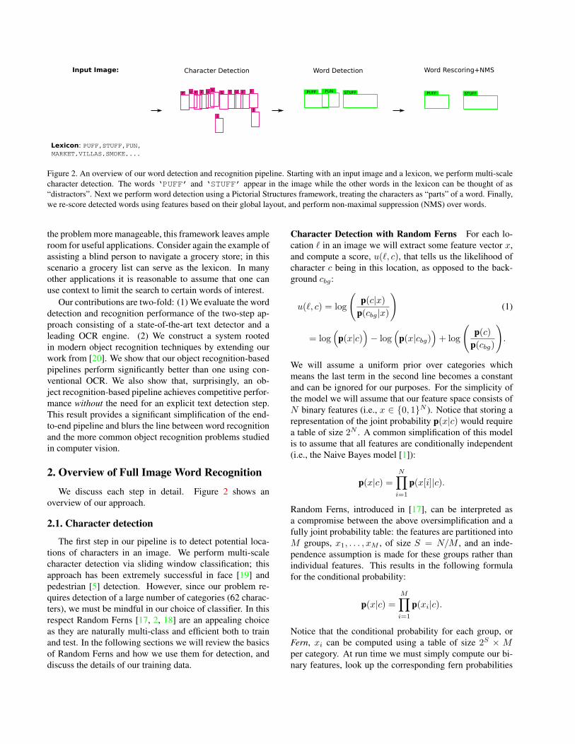
Input Image: Character Detection Word Detection Word Rescoring+NMS

UP STUFFPUFF

Figure 2. An overview of our word detection and recognition pipeline. Starting with an input image and a lexicon, we perform multi-scalecharacter detection. The words ‘PUFF’ and ‘STUFF’ appear in the image while the other words in the lexicon can be thought of as“distractors”. Next we perform word detection using a Pictorial Structures framework, treating the characters as “parts” of a word. Finally,we re-score detected words using features based on their global layout, and perform non-maximal suppression (NMS) over words.

the problem more manageable, this framework leaves ampleroom for useful applications. Consider again the example ofassisting a blind person to navigate a grocery store; in thisscenario a grocery list can serve as the lexicon. In manyother applications it is reasonable to assume that one canuse context to limit the search to certain words of interest.

Our contributions are two-fold: (1) We evaluate the worddetection and recognition performance of the two-step ap-proach consisting of a state-of-the-art text detector and aleading OCR engine. (2) We construct a system rootedin modern object recognition techniques by extending ourwork from [20]. We show that our object recognition-basedpipelines perform significantly better than one using con-ventional OCR. We also show that, surprisingly, an ob-ject recognition-based pipeline achieves competitive perfor-mance without the need for an explicit text detection step.This result provides a significant simplification of the end-to-end pipeline and blurs the line between word recognitionand the more common object recognition problems studiedin computer vision.

2. Overview of Full Image Word Recognition

We discuss each step in detail. Figure 2 shows anoverview of our approach.

2.1. Character detection

The first step in our pipeline is to detect potential loca-tions of characters in an image. We perform multi-scalecharacter detection via sliding window classification; thisapproach has been extremely successful in face [19] andpedestrian [5] detection. However, since our problem re-quires detection of a large number of categories (62 charac-ters), we must be mindful in our choice of classifier. In thisrespect Random Ferns [17, 2, 18] are an appealing choiceas they are naturally multi-class and efficient both to trainand test. In the following sections we will review the basicsof Random Ferns and how we use them for detection, anddiscuss the details of our training data.

Character Detection with Random Ferns For each lo-cation ` in an image we will extract some feature vector x,and compute a score, u(`, c), that tells us the likelihood ofcharacter c being in this location, as opposed to the back-ground cbg:

u(`, c) = log

(p(c|x)

p(cbg|x)

)(1)

= log(

p(x|c))− log

(p(x|cbg)

)+ log

(p(c)

p(cbg)

).

We will assume a uniform prior over categories whichmeans the last term in the second line becomes a constantand can be ignored for our purposes. For the simplicity ofthe model we will assume that our feature space consists ofN binary features (i.e., x ∈ {0, 1}N ). Notice that storing arepresentation of the joint probability p(x|c) would requirea table of size 2N . A common simplification of this modelis to assume that all features are conditionally independent(i.e., the Naive Bayes model [1]):

p(x|c) =N∏

i=1

p(x[i]|c).

Random Ferns, introduced in [17], can be interpreted asa compromise between the above oversimplification and afully joint probability table: the features are partitioned intoM groups, x1, . . . , xM , of size S = N/M , and an inde-pendence assumption is made for these groups rather thanindividual features. This results in the following formulafor the conditional probability:

p(x|c) =M∏i=1

p(xi|c).

Notice that the conditional probability for each group, orFern, xi can be computed using a table of size 2S × Mper category. At run time we must simply compute our bi-nary features, look up the corresponding fern probabilities

Figure 3. Top: synthetic data generated by placing a small randomcharacter (with 1 of 40 different fonts) in the center of a 48 × 48pixel patch and two neighboring characters, adding Gaussian noiseand a random affine deformation. Bottom: “real” characters fromthe ICDAR dataset. To train our character detector we generated1000 images for each character.

in stored tables, and multiply the results (or take a log andadd). In our present implementation the features consist ofapplying randomly chosen thresholds on randomly chosenentries in a HOG descriptor [5] computed at the windowlocation. This framework scales well with the number ofcategories, and has been incorporated in real-time systemsfor keypoint matching [17] and object recognition [18].

The final step of character detection is to perform non-maximal suppression (NMS). We do this separately for eachcharacter using a simple greedy heuristic (similar to what isdescribed in [9]): we iterate over all windows in the imagein descending order of their score, and if the location hasnot yet been suppressed, we suppress all of its neighbors(i.e., windows that have an overlap over some threshold).

The character detection step can be applied directly tothe image or after a generic text detector has identified re-gions of interest.

Equipped with this simple but robust classification mod-ule we must now face the task of collecting enough trainingdata to achieve good detection performance.

Synthetic Training Data Collecting a sufficiently largedataset is a typical burden of using a supervised learningmethod. However, some domains have enjoyed success bytraining and/or evaluating on synthetically generated im-ages: fingerprints [3], fluorescent microscopy images [12],keypoint deformations [17], and even pedestrians [11, 14].Beyond the obvious advantage of having limitless amountsof data, synthesizing training images allows for precise con-trol over alignment of bounding boxes – an important prop-erty that is often critical to learning a good classifier.

We synthesized about 1000 images per character using40 fonts. For each image we add some amount of Gaussiannoise, and apply a random affine deformation. Examples of

our synthesized examples are shown in Figure 3, along withexamples of “real” characters from the ICDAR dataset.

2.2. Pictorial Structures

To detect words in the image, we use the Pictorial Struc-tures (PS) [10] formulation that takes the locations andscores of detected characters as input and finds an opti-mal configuration of a particular word. More formally, letw = (c1, c2, ..., cn) be some word with n characters fromour lexicon, Li be the set of detected locations for the ith

character in w, and u(`i, ci) be the score of a particular de-tection at `i ∈ Li, computed with Eqn. (1). We seek tofind a configuration L∗ = (`∗1, . . . , `

∗n) by optimizing the

following objective function:

L∗ = argmin∀i,`i∈Li

(n∑

i=1

−u(`i, ci) +n−1∑i=1

d(`i, `i+1)

), (2)

where d(li, lj) is a pairwise cost that incorporates spatiallayout and scale similarity between two neighboring char-acters1. In practice, a tradeoff parameter is used to balancethe contributions of the two terms.

The above objective can be optimized efficiently usingdynamic programming as follows. Let D(li) be the costof the optimal placement of characters i + 1 to n with thelocation of the ith character fixed at `i:

D(li) = −u(li, ci)+ minli+1∈Li+1

d(li, li+1)+D (li+1) . (3)

Notice that total cost of the optimal configuration L∗ ismin`1∈L1 D(`1). Due to the recursive nature of D(·) wecan find the optimal configuration by first pre-computingD(`n) = −u(`n, cn) for each `n ∈ Ln and then workingbackwards toward the first letter of the word. For improvedefficiency we also include a pruning rule when performingthe minimization in Eqn. (3) by only considering locationsof `i+1 that are sufficiently spatially close to `i.

Pictorial Structures with a Lexicon. The dynamic pro-gramming procedure for configuring a single word can beextended to finding configurations of multiple words. Con-sider for example the scenario where the lexicon containsthe two words {‘ICCV’,‘ECCV’}. The value of D(`2)is the same for both words because they share the suffix‘CCV’, and can therefore be computed once and used forconfiguring both words. We leverage this by building a triestructure out of the lexicon, with all the words reversed.Figure 4 shows an example of a trie for five words, with theshaded nodes marking the beginning of words from the lex-icon (the rest of string is formed by tracing back to the root

1The deformation cost measures the deviation of a child character to theexpected location relative to its parent, which is specified as one character-width away, as in [20].

N

I

A

P

S

RI E

C

C

V

Figure 4. An example of a trie data structure built fora lexicon containing the words {‘ICCV’,‘ECCV’,‘SPAIN’,‘PAIN’,‘RAIN’}. Every node in the trie thatis the beginning of a word is shaded in gray. To efficientlyperform Pictorial Structures for all words in the lexicon, wetraverse the trie, storing intermediate configuration solutions atevery node. When a shaded node is reached, we return the optimalconfigurations for the corresponding word.

of the tree). To find configurations of the lexicon words inthe image, we traverse the trie and store intermediate solu-tions at every node. When we reach nodes labeled as words(the grayed out nodes), we return the optimal configurationsas word candidates. In practice, since an image may con-tain more than one instance of each word, we return a fewof the top configurations for each word. In the worst case,when no two words in the lexicon share a common suffix,this method is equivalent to performing the optimization foreach word separately. In practice, however, performing theoptimization jointly is typically more efficient. In the re-mainder of the paper we will refer to the above procedureas “PLEX”.

2.3. Word Re-scoring and NMS

The final step in our pipeline is to perform non-maximalsuppression over all detected words. Unfortunately, thereare a couple problems with the scores returned by PLEX.First, these scores are not comparable for words of differentlengths. The more important issue, however, is that the Pic-torial Structures objective function captures only pairwiserelationships and ignores global features of the configura-tion. While this allows for an efficient dynamic program-ming solution to finding good configurations, we would liketo capture some global information in our final step. Wetherefore re-score each word returned by PLEX in the fol-lowing manner. We compute a number of features given aword and its configuration:

• The configuration score from PLEX (i.e., cost of L∗)• Mean, median, minimum and standard deviation of

character scores (i.e., u(`i))• Standard deviation of horizontal and vertical gaps be-

tween consecutive characters• Number of characters in a word.

These features are fed into an SVM classifier, the output ofwhich becomes the new score for the word. To train the

classifier we simply run our system on the entire trainingdataset, label each returned word positive if it matches theground truth and negative otherwise, and feed these labelsand computed features into a standard SVM package2. Pa-rameters of the SVM are set using cross validation on thetraining data. Once the words receive their new scores, weperform non-maximal suppression in the same manner aswe described for character detection in Section 2.1.

The full system, implemented in Matlab, takes roughly15 seconds on average to run on a 800 × 1200 resolutionimage with lexicon size of around 50 words. We expect theruntime to be much lower with more careful engineering(e.g., [18] showed real-time performance for Ferns).

3. Experiments

In this section we present a detailed evaluation of ourPLEX pipeline, as well as a two-step pipeline consisting ofStroke Width Transform [7] (a state-of-the-art text detector)and ABBYY FineReader3 (a leading commercial OCR en-gine). We used data from the Chars74K4 dataset, introducedin [6] for cropped character classification; the ICDAR Ro-bust Reading Competition dataset [13], discussed in Section1; and Street View Text (SVT), a full image lexicon-drivenscene text dataset introduced in [20]5.

3.1. Character Classification and Detection

We begin with an evaluation of character classificationon the Chars74K-15 (where there are 15 training examplesper character class) and the ICDAR-CH (character classifi-cation sub-benchmark). We measure performance of Fernstrained on synthetic data and Ferns trained on the real im-ages from the respective datasets (labeled ‘NATIVE’). Wealso compare to previously published results of HOG+NNand ABBYY [20], as well as MKL [6].

Table 1 lists the character classification results on thetwo datasets. We see that NATIVE+FERNS outperformsother methods on the ICDAR-CH dataset. However, itsperformance on the Chars74K-15 benchmark is below thatof previous results using HOG+NN. Upon further inspec-tion, we noticed significant similarity between the images inthe training and testing sets from Chars74K (in some casesnear duplicates) which work to the advantage of a Near-est Neighbor classifier. In contrast, the training and testingsplit in ICDAR-CH was done on a per image basis, makingit highly unlikely to have near duplicates across the split –this helps account for the drop in performance of HOG+NNon ICDAR-CH. Finally, we see that training on purely syn-

2http://www.csie.ntu.edu.tw/˜cjlin/libsvm/3http://finereader.abbyy.com4http://www.ee.surrey.ac.uk/CVSSP/demos/

chars74k/5The dataset has undergone revision since originally introduced.

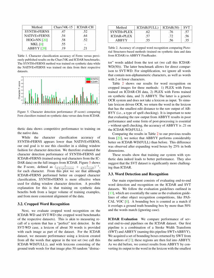
Method Chars74K-15 ICDAR-CHSYNTH+FERNS .47 .52NATIVE+FERNS .54 .64

HOG+NN [20] .58 .52MKL [6] .55 -

ABBYY [20] .19 .21

Table 1. Character classification accuracy of Ferns versus previ-ously published results on the Chars74K and ICDAR benchmarks.The SYNTH+FERNS method was trained on synthetic data whilethe NATIVE+FERNS was trained on data from their respectivedatasets.

0 1 2 3 4 5 6 7 8 9 A B C D E F G H I J K L M N O P Q R S T U V W X Y Z0

0.1

0.2

0.3

0.4

0.5

0.6

0.7

0.8

Chara

cte

r F

−score

SYNTH

ICDAR

Figure 5. Character detection performance (F-score) comparingFern classifiers trained on synthetic data versus data from ICDAR.

thetic data shows competitive performance to training onthe native data.

While the character classification accuracy ofSYNTH+FERNS appears lower than NATIVE+FERNS,our end goal is to use this classifier in a sliding windowfashion for character detection. We therefore evaluated thecharacter detection performance of SYNTH+FERNS andICDAR+FERNS (trained using real characters from the IC-DAR data) on the full images from ICDAR. Figure 5 showsthe F-score, defined as ( 1

0.5×precision + 10.5×recall )

−1,for each character. From this plot we see that althoughICDAR+FERNS performed better on cropped characterclassification, SYNTH+FERNS is more effective whenused for sliding window character detection. A possibleexplanation for this is that training on synthetic databenefits both from a larger volume of training examples,and from more consistent alignment of the data.

3.2. Cropped Word Recognition

Next, we evaluate cropped word recognition on theICDAR-WD and SVT-WD (the cropped word benchmarksof the respective datasets). This is akin to measuring re-call of a system that has a “perfect” text detector. In theSVT-WD case, a lexicon of about 50 words is providedwith each image as part of the dataset. For the ICDARdataset, we measure performance using a lexicon createdfrom all the words that appear in the test set (we call thisICDAR-WD(FULL)), and with lexicons consisting of theground truth words for that image plus 50 random “distrac-

Method ICDAR(FULL) ICDAR(50) SVTSYNTH+PLEX .62 .76 .57ICDAR+PLEX .57 .72 .56

ABBYY .55 .56 .35

Table 2. Accuracy of cropped word recognition comparing Picto-rial Structures-based methods (trained on synthetic data and datafrom ICDAR) to ABBYY FineReader.

tor” words added from the test set (we call this ICDAR-WD(50)). The latter benchmark allows for direct compar-ison to SVT-WD. For simplification, we ignore all wordsthat contain non-alphanumeric characters, as well as wordswith 2 or fewer characters.

Table 2 shows our results for word recognition oncropped images for three methods: 1) PLEX with Fernstrained on ICDAR-CH data, 2) PLEX with Ferns trainedon synthetic data, and 3) ABBYY. The latter is a genericOCR system and does not take a lexicon as input. To simu-late lexicon driven OCR, we return the word in the lexiconthat has the smallest edit distance to the raw output of AB-BYY (i.e., a type of spell checking). It is important to notethat evaluating the raw output from ABBYY results in poorperformance and some form of post-processing is essential– without spell checking, the accuracy of ABBYY is .21 onthe ICDAR-WD(FULL).

Comparing the results in Table 2 to our previous resultsfrom [20], we notice that ABBYY performs considerablybetter on ICDAR-WD(FULL) than before. This differencewas observed after expanding word boxes by 25% in bothdimensions.

These results show that training our system with syn-thetic data indeed leads to better performance. They alsosuggest that the SVT dataset is significantly more challeng-ing than ICDAR.

3.3. Word Detection and Recognition

Our main experiment consists of evaluating end-to-endword detection and recognition on the ICDAR and SVTdatasets. We follow the evaluation guidelines outlined in[13], which are essentially the same as the evaluation guide-lines of other object recognition competitions, like PAS-CAL VOC [8]. A bounding box is counted as a match ifit overlaps a ground truth bounding box by more than 50%and the words match (ignoring case).

ICDAR Evaluation We compare performance of sev-eral end-to-end pipelines on the ICDAR dataset. Our firstpipeline is a combination of a Stroke Width Transform(SWT) and ABBYY (naming this pipeline SWT+ABBYY).We acquired a set of bounding boxes returned by SWT fromthe authors of [7]; these regions are then fed into ABBYY.As we did before, we correct results from ABBYY by con-verting its output to the word in the lexicon with the smallest

0 0.1 0.2 0.3 0.4 0.5 0.6 0.7 0.80.5

0.6

0.7

0.8

0.9

1

K = 5

Recall

Pre

cis

ion

SWT+ABBYY [0.62]

SWT+PLEX [0.71]

SWT+PLEX+R [0.71]

PLEX [0.69]

PLEX+R [0.72]

0 0.1 0.2 0.3 0.4 0.5 0.6 0.7 0.80.5

0.6

0.7

0.8

0.9

1

K = 20

Recall

Pre

cis

ion

SWT+ABBYY [0.61]

SWT+PLEX [0.69]

SWT+PLEX+R [0.70]

PLEX [0.62]

PLEX+R [0.69]

0 0.1 0.2 0.3 0.4 0.5 0.6 0.7 0.80.5

0.6

0.7

0.8

0.9

1

K = 50

Recall

Pre

cis

ion

SWT+ABBYY [0.60]

SWT+PLEX [0.67]

SWT+PLEX+R [0.68]

PLEX [0.56]

PLEX+R [0.65]

Figure 6. Precision and recall of end-to-end word detection and recognition methods on the ICDAR dataset. Results are shown withlexicons created with 5, 20, and 50 distractor words. F-scores are shown in brackets next to pipeline name.

edit distance. In this case, we throw out all bounding boxesfor which ABBYY returns an empty string, or for whichthe smallest edit distance to a lexicon word is above somethreshold – this helps reduce the number of false positivesfor this system.

Next, we apply PLEX to full images without a text de-tection step (named PLEX). Finally, we combine SWT withPLEX as the reading engine (named SWT+PLEX). This hy-brid pipeline serves as a sanity check to see if text detec-tion improves results of PLEX. To show the effect of there-scoring technique presented in Section 2.3, we evaluatethe latter two pipelines with and without this step (adding‘+R’ to the name when re-scoring is used). Motivated byour earlier experiments, we all PLEX-based systems weretrained on synthetic data.

We construct a lexicon for each image by taking theground truth words that appear in that image and adding Kextra distractor words chosen at random from the test set, aswell as filtering short words, as in the previous experiment.

Figure 8 shows select examples of output; Figure 6shows precision and recall plots for different values of K aswe sweep over a threshold on scores (or maximum edit dis-tance for ABBYY, as described above). From these results,we make the following observations. (1) Re-scoring signifi-cantly improves performance of PLEX, especially for largerlexicons. (2) The performance of PLEX-based pipelines issignificantly better than SWT+ABBYY. While the gap inF-scores of these methods shrinks as the lexicon increases,the PLEX based systems obtain a considerably higher recallat high precision points in all cases. (3) PLEX+R, a systemthat does not rely on explicit text detection, is not only com-parable to SWT+PLEX+R, but actually outperforms it forsmaller length lexicons.

While an explicit text detection step could in principleimprove the precision of a system, the recall is also lim-ited by that of the text detector. Improving the recall ofsuch a two stage pipeline would therefore necessitate im-proving the recall of text detection. Upon further examina-tion of our results, we found a strong positive correlationbetween the words that ABBYY was able to read and thewords that were detected by the SWT detector. Recall thatin the cropped word experiment, ABBYY achieved .56 ac-

0 0.05 0.1 0.15 0.2 0.25 0.3 0.35 0.4 0.45 0.50

0.2

0.4

0.6

0.8

1

RecallP

recis

ion

PLEX [0.27]

PLEX+R [0.38]

Figure 7. Precision and recall of end-to-end word detection andrecognition methods on the Street View Text dataset. F-scores areshown in brackets next to pipeline name.

curacy on the ICDAR-WD(50) benchmark (correctly read-ing 482 words). In the end-to-end benchmark of ICDARwith K = 50, SWT+ABBYY correctly read 438 words(very close to its performance on cropped words, whichsimulates a “perfect” text detector). This shows that im-proving the recall of SWT would not have a big impact onthe performance of SWT+ABBYY, unless ABBYY was im-proved as well.

While ABBYY is a black box, the PLEX pipeline is con-structed using computer vision techniques that are well un-derstood and constantly improved by the community. Webelieve this paves a clearer path towards improving readingaccuracy.

The work of [16] reported word recognition results onthe ICDAR dataset of 0.42/0.39/0.40, for precision, recalland F-score. In our experiments, we created word lists forevery image, however word lists were not provided in theexperiments in [16], making the results not directly compa-rable. The closest comparison in our framework is to pro-vide the entire ground truth set (> 500) as a word list to eachtest image. In that case, our PLEX+R pipeline achieves0.45/0.54/0.51.

SVT Evaluation For the SVT dataset, we evaluated onlyPLEX and PLEX+R because we were unable to obtainSWT output for this data (and the original implementationis not publicly available). Recall that this dataset comeswith a lexicon for each image (generated from local busi-

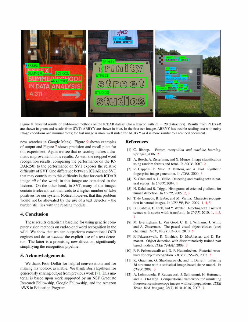
Figure 8. Selected results of end-to-end methods on the ICDAR dataset (for a lexicon with K = 20 distractors). Results from PLEX+Rare shown in green and results from SWT+ABBYY are shown in blue. In the first two images ABBYY has trouble reading text with noisyimage conditions and unusual fonts; the last image is more well suited for ABBYY as it is more similar to a scanned document.

ness searches in Google Maps). Figure 9 shows examplesof output and Figure 7 shows precision and recall plots forthis experiment. Again we see that re-scoring makes a dra-matic improvement in the results. As with the cropped wordrecognition results, comparing the performance on the IC-DAR(50) to the performance on SVT exposes the relativedifficulty of SVT. One difference between ICDAR and SVTthat may contribute to this difficulty is that for each ICDARimage all of the words in that image are contained in thelexicon. On the other hand, in SVT, many of the imagescontain irrelevant text that leads to a higher number of falsepositives for our system. Notice, however, that this problemwould not be alleviated by the use of a text detector – theburden still lies with the reading module.

4. ConclusionThese results establish a baseline for using generic com-

puter vision methods on end-to-end word recognition in thewild. We show that we can outperform conventional OCRengines and do so without the explicit use of a text detec-tor. The latter is a promising new direction, significantlysimplifying the recognition pipeline.

5. AcknowledgementsWe thank Piotr Dollar for helpful conversations and for

making his toolbox available. We thank Boris Epshtein forgenerously sharing output from previous work [7]. This ma-terial is based upon work supported by an NSF GraduateResearch Fellowship, Google Fellowship, and the AmazonAWS in Education Program.

References[1] C. Bishop. Pattern recognition and machine learning.

Springer, 2006. 2[2] A. Bosch, A. Zisserman, and X. Munoz. Image classification

using random forests and ferns. In ICCV, 2007. 2[3] R. Cappelli, D. Maio, D. Maltoni, and A. Erol. Synthetic

fingerprint-image generation. In ICPR, 2000. 3[4] X. Chen and A. L. Yuille. Detecting and reading text in nat-

ural scenes. In CVPR, 2004. 1[5] N. Dalal and B. Triggs. Histograms of oriented gradients for

human detection. In CVPR, 2005. 2, 3[6] T. de Campos, B. Babu, and M. Varma. Character recogni-

tion in natural images. In VISAPP, Feb. 2009. 1, 4, 5[7] B. Epshtein, E. Ofek, and Y. Wexler. Detecting text in natural

scenes with stroke width transform. In CVPR, 2010. 1, 4, 5,7

[8] M. Everingham, L. Van Gool, C. K. I. Williams, J. Winn,and A. Zisserman. The pascal visual object classes (voc)challenge. IJCV, 88(2):303–338, 2010. 5

[9] P. Felzenszwalb, R. Girshick, D. McAllester, and D. Ra-manan. Object detection with discriminatively trained partbased models. IEEE TPAMI, 2009. 3

[10] P. F. Felzenszwalb and D. P. Huttenlocher. Pictorial struc-tures for object recognition. IJCV, 61:55–79, 2005. 3

[11] K. Grauman, G. Shakhnarovich, and T. Darrell. Inferring3d structure with a statistical image-based shape model. InCVPR, 2008. 3

[12] A. Lehmussola, P. Ruusuvuori, J. Selinummi, H. Huttunen,and O. Yli-Harja. Computational framework for simulatingfluorescence microscope images with cell populations. IEEETrans. Med. Imaging, 26(7):1010–1016, 2007. 3

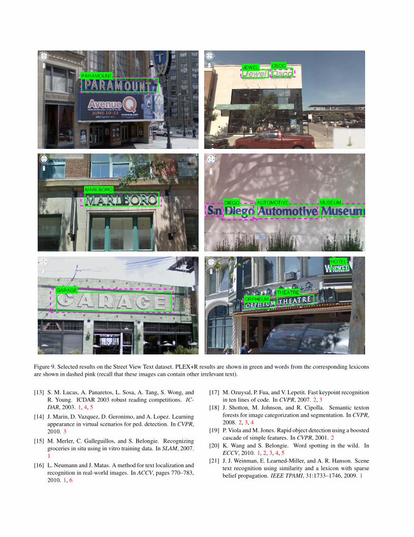
Figure 9. Selected results on the Street View Text dataset. PLEX+R results are shown in green and words from the corresponding lexiconsare shown in dashed pink (recall that these images can contain other irrelevant text).

[13] S. M. Lucas, A. Panaretos, L. Sosa, A. Tang, S. Wong, andR. Young. ICDAR 2003 robust reading competitions. IC-DAR, 2003. 1, 4, 5

[14] J. Marin, D. Vazquez, D. Geronimo, and A. Lopez. Learningappearance in virtual scenarios for ped. detection. In CVPR,2010. 3

[15] M. Merler, C. Galleguillos, and S. Belongie. Recognizinggroceries in situ using in vitro training data. In SLAM, 2007.1

[16] L. Neumann and J. Matas. A method for text localization andrecognition in real-world images. In ACCV, pages 770–783,2010. 1, 6

[17] M. Ozuysal, P. Fua, and V. Lepetit. Fast keypoint recognitionin ten lines of code. In CVPR, 2007. 2, 3

[18] J. Shotton, M. Johnson, and R. Cipolla. Semantic textonforests for image categorization and segmentation. In CVPR,2008. 2, 3, 4

[19] P. Viola and M. Jones. Rapid object detection using a boostedcascade of simple features. In CVPR, 2001. 2

[20] K. Wang and S. Belongie. Word spotting in the wild. InECCV, 2010. 1, 2, 3, 4, 5

[21] J. J. Weinman, E. Learned-Miller, and A. R. Hanson. Scenetext recognition using similarity and a lexicon with sparsebelief propagation. IEEE TPAMI, 31:1733–1746, 2009. 1