HAL Id: tel-01406637https://hal.archives-ouvertes.fr/tel-01406637

Submitted on 1 Dec 2016

HAL is a multi-disciplinary open accessarchive for the deposit and dissemination of sci-entific research documents, whether they are pub-lished or not. The documents may come fromteaching and research institutions in France orabroad, or from public or private research centers.

L’archive ouverte pluridisciplinaire HAL, estdestinée au dépôt et à la diffusion de documentsscientifiques de niveau recherche, publiés ou non,émanant des établissements d’enseignement et derecherche français ou étrangers, des laboratoirespublics ou privés.

Endogenous Business Cycles and Hysteresis. APost-Keynesian, Agent-Based Approach

Federico Bassi

To cite this version:Federico Bassi. Endogenous Business Cycles and Hysteresis. A Post-Keynesian, Agent-Based Ap-proach. Economics and Finance. Università degli Studi di Roma ”La Sapienza”; Université Paris 13,Sorbonne Paris Cité, 2016. English. �tel-01406637�

Endogenous Business Cycles and Hysteresis.

A Post-Keynesian, Agent-Based Approach

Federico Bassi

PhD in “Economia e Finanza Internazionale”

Università degli Studi di Roma “La Sapienza”

Joint supervision agreement with

“Centre d’Economie de Paris Nord” (CEPN, UMR CNRS 7234)

Ecole Doctorale Erasme, Université “Paris 13, Sorbonne Paris Cité”

Dissertation defence: 09 June 2016

Supervisors:

Dany Lang, CEPN, Université “Paris 13, Sorbonne Paris Cité”

Luca Zamparelli, Università degli Studi di Roma “La Sapienza”

Committee members:

Marc Lavoie, Université “Paris 13, Sorbonne Paris Cité”

Mark Setterfield, New School for Social Research

Andrea Roventini, Scuola Superiore Sant’Anna di Pisa

Massimiliano Tancioni, Università degli Studi di Roma “La Sapienza”

Dany Lang, CEPN, Université “Paris 13, Sorbonne Paris Cité”

Luca Zamparelli, Università degli Studi di Roma “La Sapienza”

A Livia e Arianna, e al loro impagabile sorriso

Acknowledgements

I take this opportunity to sincerely acknowledge my supervisors, Professor Dany Lang and

Professor Luca Zamparelli, without whom I never would have realized this thesis. Thanks to

them, I could enjoy the possibility to work between the department of economics of the

University of Rome “La Sapienza” and the “Centre d’Economie de Paris Nord” (CEPN) of

the University “Paris 13, Sorbonne Paris Cité”, benefiting from the invaluable cultural

enrichment of this experience.

I would like also to thank Professor Marc Lavoie, Professor Mark Setterfield, Professor

Andrea Roventini and Professor Massimiliano Tancioni for honouring me by taking part in

the thesis committee.

My thesis benefited from many different contributions. I wish to thank all those professors of

the PhD School of Economics of “La Sapienza” who accepted to give us classes during our

first year in Rome, providing us with fundamental tools to pursue our research project. I wish

also to express my gratitude to all members of the CEPN for hosting me, particularly to

Michael Lainé, Professor Angel Asensio, Professor Jonathan Marie and Professor Sébastien

Charles, with whom I had extraordinary talks and discussions which interest went far beyond

the thesis itself; Professor Cédric Durand, for his extremely helpful comments and

suggestions during the early stages of my thesis. I am also particularly grateful to Professor

Steven Pressman, for his helpful comments concerning the 1st chapter of the thesis, and his

encouragement to pursue in this project.

In these last two years, I had the possibility to present my works in different conferences and

summer schools, and benefiting from helpful feedbacks. I wish to acknowledge the

participants at the 26th

annual conference of the European Association for Evolutionary

Political Economy (EAEPE), particularly Professor Paolo Piacentini and Professor Carlo

D’Ippoliti, who provided useful remarks and suggestions concerning the 2nd

chapter of this

thesis; the participants and organizers of the 2nd

Limerick Winter School on AB-SFC

modelling, namely Antoine Godin, Eugenio Caverzasi, Alessandro Caiani and Professor

Stephen Kinsella, who gave me the opportunity to present my ongoing research, and have

important feedbacks. This school was extremely profitable for my thesis and, in particular, for

the 4th

chapter, which also benefited from the discussions with Pascal Seppecher and

Professor Gérard Ballot, while presenting my work at the 2nd

conference of the Modelling and

Analysis of Complex Monetary Economies (MACME) network.

I wish to express my gratitude to my Italian and French colleagues, who contributed to make

this experience unforgettable. A special thank to Dario Guarascio, Davide Del Prete, Valerio

Leone Sciabolazza, Francesco Zaffuto, Gaetano Tarcisio Spartà and Flavio Santi, with whom

I shared a wonderful year in Rome; to Idir Hafrad, the first that I met in “Paris 13” and the

one I could fall back on at any moment; to Félix Boggio Ewangé-Epée, to whom I can only

reproach his faith in a long run normal rate of capacity utilization; Serge Herbillon-Leprince,

for the long (very long, indeed!) discussions we had in these last years in Paris and for

travelling thousands of miles to attend my thesis’ defence, together with Louison Cahen-

Fourot and Bruno Carballa Smichowski, who also deserve my full gratitude. A special thank

also to Sy-Hoa Ho, Alberto Cardaci, Matteo Cavallaro, Marco Ranaldi, Simon Nadel, Marta

Fana, Giuseppe Di Molfetta and all those that I did not mention and that contributed to make

this experience in Paris unforgettable.

Needless to say, a very personal thought goes to Daniela, Guido, Natalia, Ruggero, Arianna

and Livia, whose presence and support were the real condicio sine qua non of this

achievement.

Index

General introduction ............................................................................................................................... 7

1. Asymptotic stability, path-dependence and hysteresis. A literature review on macro-dynamic

properties of macroeconomic modelling .............................................................................................. 13

1.1. The Natural rate hypothesis: a historical perspective ........................................................... 13

1.1.1. Homeostasis and asymptotic stability ........................................................................... 13

1.1.2. The Natural rate of unemployment and its policy implications .................................... 14

1.1.3. The Non-accelerating inflation rate of unemployment and its policy implications ...... 18

1.1.4. NRU Vs NAIRU: differences and similarities .................................................................. 22

1.1.5. Epistemological and theoretical remarks concerning the NAIRU and the NRU ............ 24

1.2. Path-dependency, supply-side time variance and hysteresis in the mainstream approach . 28

1.2.1. Time irreversibility and path-dependence: an empirical evidence ............................... 28

1.2.2. Supply side shocks, equilibrium multiplicity and hysteresis ......................................... 32

1.2.3. Hysteresis as unit-root persistence ............................................................................... 35

1.2.3.1. Epistemological assumptions ................................................................................ 35

1.2.3.2. Theoretical models of hysteresis ........................................................................... 36

1.2.3.3. Empirical models of unit-root persistence ............................................................ 40

1.3. Alternative approaches to hysteresis: cumulative non neutrality, discontinuous adjustments

and structural change ........................................................................................................................ 43

1.3.1. Persistence Vs structural change................................................................................... 43

1.3.2. Hysteresis as a theory of structural change .................................................................. 44

1.3.3. Sunk costs, discontinuous adjustments and hysteresis: an endogenous structural

change approach ........................................................................................................................... 47

1.3.4. Genuine hysteresis Vs unit root: non linearity, selective memory and remanence ..... 55

1.3.5. Policy implications and concluding remarks ................................................................. 58

2. Discontinuous entry and exit decisions. Long run non-neutrality of demand policies ................. 62

2.1. Introduction ........................................................................................................................... 62

2.2. A “new consensus” monetary model with genuine hysteresis ............................................. 67

2.2.1. The standard “new consensus” model .......................................................................... 67

2.2.2. Potential output and “genuine” hysteresis ................................................................... 68

2.3. Productive capacity adjustments: structural change Vs temporary persistence ................ 72

2.3.1. Permanent effects of temporary shocks and long run non neutrality of economic

policies….. ...................................................................................................................................... 73

2.3.2. Policy effectiveness in linear hysteresis-augmented “new consensus” models ........... 76

2.4. Economic policy implications of “genuine” hysteresis and concluding remarks .................. 82

Appendix 2.1: parameters’ value ...................................................................................................... 85

3. Sunk costs effects, discontinuous investment decisions and fully endogenous degrees of capacity

utilization. A Post-Keynesian micro-foundation .................................................................................... 86

3.1. Introduction ........................................................................................................................... 86

3.2. A simple path-dependent agent-based PKK model of growth and distribution ................... 93

3.2.1. Sunk costs, strategic decisions and switching values .................................................... 95

3.2.2. Effective demand, expectations and the rate of capacity utilization ............................ 96

3.2.3. Investment decisions and capital accumulation ........................................................... 98

3.2.4. Income distribution, employment and consumption decisions .................................. 100

3.2.5. Dynamics of the Agent-Based model .......................................................................... 103

3.3. Emergent properties and reaction to shocks ...................................................................... 104

3.3.1. The “paradox of costs” and the consequence of cuts in the real wage ...................... 105

3.3.2. The “paradox of thrift” and the Fisher effect .............................................................. 107

3.3.3. Animal spirits and the propensity to invest ................................................................ 110

3.4. Concluding remarks ............................................................................................................. 111

Appendix 3.1: values of parameters................................................................................................ 115

Appendix 3.2: sensitivity analysis .................................................................................................... 116

4. Coerced investments, growth/safety trade-off and the stabilizing role of demand policies. An

Agent-based stock flow consistent model of endogenous business cycles and structural change .... 120

4.1. Introduction ......................................................................................................................... 120

4.2. The model ............................................................................................................................ 129

4.2.1. Structure and timing of events .................................................................................... 129

4.2.2. Capital goods firms ...................................................................................................... 131

4.2.3. Consumption goods firms ........................................................................................... 132

4.2.3.1. Production and productivity ................................................................................ 132

4.2.3.2. Wages, mark-up and pricing ................................................................................ 133

4.2.3.3. Investment decisions ........................................................................................... 134

4.2.3.4. Profits, retained earnings and loans .................................................................... 135

4.2.4. Households .................................................................................................................. 137

4.2.5. Commercial bank ......................................................................................................... 138

4.2.6. Central bank ................................................................................................................ 139

4.2.7. Government ................................................................................................................ 140

4.3. Simulations and results of the model .................................................................................. 141

4.3.1. Results of the simulations in the irreversible-investments scenarios ......................... 142

4.3.2. Statistical emergent properties: stationarity and non-ergodicity ............................... 145

4.4. Concluding remarks ............................................................................................................. 152

Appendix 4.2.1: balance sheet ........................................................................................................ 157

Appendix 4.2.2: transactions’ matrix .............................................................................................. 158

Appendix 4.3: graphical representation of the circuit .................................................................... 159

Appendix 4.4.1 : monetary flows diagram ...................................................................................... 160

Appendix 4.4.2: “real” flows diagram ............................................................................................. 161

General conclusion .............................................................................................................................. 162

References ........................................................................................................................................... 167

7

General introduction

Since the marginalist revolution of the 19th

century, mainstream economic theory has

historically developed around the concept of “natural” equilibrium (Lang, 2009). By assuming

that the economic structure remains utterly invariant, business cycles have always been

analysed through a strict dichotomy between the demand side, which is supposed to be

representative of what economists define as the “short run”, and the supply side, which is

supposed to represent the “long run” centre of gravity. To the extent that the supply side is

strictly independent from the demand side, long lasting deviations of the economy from the

original steady state are interpreted as the consequence of exogenous structural changes

taking place directly in the supply side. In absence of such exogenous shifts, demand shock

must necessary cancel out in the end, when the economy adjusts to the “natural” equilibrium,

by leaving no trace on the structure of the economy.

This theoretical framework has been radically questioned in the 1980s, in the wake of

the oil shocks and the consequential deflationary policies implemented in most European

countries (Blanchard & Summers, 1986; Cross, 1987). The empirical evidence of a strong

persistence of high rates of unemployment, despite the temporary nature of the shocks,

suggested the need for a new macro-dynamic framework alternative to the Natural Rate

Hypothesis (NRH). There were two macro elements at stake: the more complex relationship

between demand and the supply side, which are supposed to influence each other; and the

non-reversibility of the consequences of shocks on the structure of the economy, namely

hysteresis.

Not surprisingly, the financial crisis that burst out in 2008 raised a new emphasis on

this topic. The evidence of the long run damages caused by the meltdown in most European

countries on one hand (Ball, 2014), and the inadequacy of the mainstream to account for these

permanent losses of productive capacity on the other hand (Cross et al, 2012), confirmed the

failure of the neoclassical paradigm of asymptotic stability to provide a convincing

explanation of real-world macro-dynamics. In particular, a growing literature is putting

forward the hypothesis that large and/or long lasting negative shocks, such as the 2008’s

financial crisis, leave a permanent scarce on the economy (Blanchard & Summers, 1986; Ball

et al, 1999; Cerra & Saxena, 2008; Ball, 2009; Schettkat & Sun, 2009; Cross et al, 2012).

8

There is still no theoretical consensus as regards how demand shocks impact on long run

trajectories, and which modelling strategies are most appropriate to represent hysteresis. In

particular, there are two main frameworks to explain and analyze the permanent impact of

transitory shocks. According to the first one, hysteresis relies on the concept of unit/zero root

persistence (Blanchard & Summers, 1986; Ball et al, 1999; Kapadia, 2005; Lavoie, 2006;

Ball, 2009; Schettkat & Sun, 2009; Fontana & Passarella, 2014; Kienzler & Schmid, 2014). In

this framework, hysteresis implies an exceptional persistence in disequilibrium adjustment

that can be properly represented by non-stationary processes. The mean reverting property of

these models – when properly differentiated – is one of the main reasons of their success,

since it allows working on systems of linear equations that are easily testable through standard

linear econometrics techniques. Furthermore, when introduced into broader mainstream

macroeconomic frameworks, these models of hysteresis substantially validate most of the

policy implications that apply also to non-hysteretic systems, at least in the long run (Kapadia,

2005; Kienzler & Schmid, 2014).

An alternative approach consists of representing hysteresis as a source of structural

change (Roed, 1997; Setterfield, 1998, 2008). By abandoning the mainstream dichotomy

between strictly stationary processes, characterized by a deterministic trend and temporary

deviations, and strictly non-stationary processes, characterized on the contrary by a stochastic

trend, these approaches focus on the possibility that demand fluctuations trigger structural

changes that permanently affect the long run trend. In this framework, hysteresis is no longer

related to non-stationarity but, generally speaking, to non-ergodicity.

The model of genuine hysteresis is part of this broader class of non-ergodic processes.

Firstly theorized by J.A. Ewing in the 19th

century while studying the properties of ferric

metals submitted to a process of magnetization and de-magnetization, genuine hysteresis is

the consequence of non-linear and discontinuous adjustments at the micro level that generate

non-ergodic aggregate dynamics (Cross, 1993B, 1994; Amable et al, 1994, 1995; Piscitelli et

al, 2000). The model of genuine hysteresis provides a macro-dynamic framework alternative

to the unit root approach that is able to fit with empirical time-series, and which is able to

provide an alternative analysis of business cycles and growth paths. Indeed, since the

statistical properties of this model are radically opposed to the statistical properties of both

traditional asymptotically stable models and random walks, namely as regards mean reversion

(De Peretti, 2007), proving the consistency of the model with empirical time-series allows to

credibly reject the NRH in favour of a more general theory of hysteresis that does not

9

necessary require non-stationarity. Despite the large explanatory power of the genuine

hysteresis model, which fits with virtually all time series, either stationary or non stationary,

there are no systematic attempts to introduce this framework into broader macroeconomic

models in order to analyze the emergent policy conclusions. The aim of this thesis is to

formally introduce genuine hysteresis into a Post Keynesian macroeconomic model in order

to analyze the consequences and the emerging policy implications, on a set of macroeconomic

aggregate variables, of introducing non-linearity and discontinuity in investment decisions. In

particular, by referring to the theories of sunk costs effects (Arker & Blumer, 1985; Garland,

1990) and coerced investments (Crotty, 1993), it provides a plausible micro foundation for

investment decisions that might explain how aggregate structural changes can emerge

endogenously from the aggregation of multiple and heterogeneous discontinuous decisions at

the micro level. Furthermore, by relaxing some of the standard assumptions of the model, it

aims at generalizing the application and validity of the model to more complex frameworks.

The recent development of agent-based computational techniques (ACE hereafter)

appears as the most appropriate methodological framework to integrate genuine hysteresis

into broader macroeconomic models. In this approach, aggregate results emerge

endogenously by the aggregation of multiple and heterogeneous micro behaviours that are

fully decentralized and independent from equilibrium constraints (Fagiolo & Roventini,

2012). By simulating a sequence of interactions among multiple and heterogeneous agents,

within a specific institutional framework that determines the nature and the intensity of such

interactions, the agent-based sequential approach is characterized by a large degree of

endogeneity that allows running a simultaneous analysis of both the micro-to-macro and the

macro-to-micro properties of the model. Therefore, introducing the genuine hysteresis

framework into a broader agent-based model allows performing an integrated analysis of

business cycles and growth trajectories by taking into account the feedbacks mechanisms that

run from aggregate outcomes to micro behaviours. Furthermore, it allows analyzing the

impact of institutions and economic policies in an artificial economic environment

characterized by discontinuity and non-linearity of investment decisions.

The thesis is organized as follows. Chapter 1 focuses on the macroeconomic debate

about asymptotic stability, unit root persistence and structural changes. In the first part

(section 1.1) it provides a literature review about the Natural rate of unemployment (NRU)

and the Non-accelerating inflation rate of unemployment (NAIRU), by focusing particularly

on the common properties of these models, namely the short run-long run dichotomy that

10

follows from asymptotic stability and time-independence. In the second part (section 1.2) of

the chapter we provide a literature review about the theoretical developments in mainstream

macroeconomics, namely the NAIRU framework, in order to take the empirical evidence of

unemployment persistence and path-dependence into account. In particular, this part focuses

on multiple equilibria, supply-side time variance and unit root persistence, by analyzing the

theoretical and epistemological implications of these frameworks on the short run-long run

dichotomy. In the third and last part (section 1.3) of the chapter we develop a literature review

of the different theories of hysteresis based on the concept of structural change, by focusing

specifically on the model of genuine hysteresis with its macro-dynamic implications.

Chapter 2 is a simple application of the genuine model of hysteresis to a “new

consensus” macroeconomic model (NCM). After recalling the literature on unit root

persistence and introducing the literature on NCM models, the first part of the chapter (section

2.1) focuses on the existing literature on potential output hysteresis and the monetary policy

implications in the NCM framework. When introducing unit root persistence in “new

consensus” monetary models, although supply side transitory shocks have permanent effects

demand shocks do cancel out if monetary authorities successfully target a fixed inflation rate

and the market clearing natural rate of interest. The second part of the chapter (sections 2.2

and 2.3) develops a “new consensus” model with genuine hysteresis in order to show that

discontinuous entry and exit decisions of firms imply the impossibility for a monetary

authority that follows an inflation target to systematically prevent permanent potential output

losses in the wake of transitory demand shocks. For instance, according to the initial state of

the economy, the amplitude of shocks and the reactivity of the monetary authority, temporary

shocks might imply a shift to a new equilibrium still characterized by steady inflation and a

natural rate of interest, but producing a different level of equilibrium output. The last part of

the chapter (section 2.5) concludes on macro-dynamic implications and policy conclusions. In

this framework, for instance, there is no fixed point that can be considered as a long run

centre of gravity, the equilibrium being fundamentally endogenous and unpredictable.

Discretionary fiscal and monetary policies are necessary to push the economy towards more

efficient trajectories.

Chapter 3 extends the model of chapter 2 in an agent-based framework by increasing

the degree of decentralization and introducing capital accumulation decisions. For instance,

the model of chapter 2 assumed a binary choice between entry and exit with a fixed capital

stock. By referring to the Post-Keynesian/Kaleckian theory of investment and savings, this

11

chapter develops a micro-founded model of growth and distribution characterized by multiple

and heterogeneous firms that take independent and decentralized investment decisions. In he

first part of the chapter (section 3.1), we introduce the contemporary debate within heterodox

schools of thought as regards the long run endogeneity of the rate of capacity utilization and

related properties, namely the paradoxes of costs and thrift (Rowthorn, 1981). The second part

of the chapter (sections 3.2 and 3.3) develops a neo-Kaleckian model of growth with

decentralized and discontinuous investment decisions and illustrates the main properties of the

model, namely the long run validity of the paradoxes of costs and thrift; the long run influence

of animal spirits on capital accumulation; the permanent effects of transitory shocks on the

rate of growth. In particular, we show that, contrarily to standard genuine hysteresis models

that assume an exogenous sequence of input shocks, this model provides an endogenous input

that exhibits hysteresis in the wake of transitory shocks. The third part of the chapter (section

3.4) concludes on the economic and economic policy implications of the model, namely the

endogeneity of the rates of capacity utilization, capital accumulation and unemployment in the

long run and the recessionary effects of austerity policies as long as they impact on income

distribution, on households’ saving decisions and firms’ animal spirits.

Chapter 4 extends the model of chapter 3 by further increasing the degree of

decentralization and complexifying the macroeconomic structure. The first part of the chapter

(section 4.1) introduces the debate on capacity adjustment and investment decisions in

Dynamic stochastic general equilibrium (DSGE), Real business cycle (RBC) and Agent-based

(AB) models, by focusing in particular on the way non-linear and discontinuous investment

functions have been integrated in these frameworks and the underlying theory of sunk costs.

This part of the chapter introduces a broader theory of sunk costs based on the concepts of

sunk costs effects (Arkes & Blumer, 1985; Garland, 1990) and coerced investments (Crotty,

1993) in a theoretical framework characterized by a net separation between management and

ownership (Crotty, 1993; Jensen, 1993; Schoenberger, 1994; Clark & Wrigley, 1997). The

second part of the chapter (sections 4.2 and 4.3) develops an Agent-based, stock flow

consistent (AB-SFC) model with sunk costs effects and coerced investments, and analyzes its

economic and macro-dynamic properties. It is shown that, in this framework, fiscal and

monetary regimes determine not only the amplitude of fluctuations but also the long run

trajectories. In particular, restrictive fiscal and monetary policies dramatically increase the

instability of the economy by triggering larger fluctuations and endogenous structural

changes. Expansionary fiscal and monetary policies play on the contrary a successful

12

countercyclical effect by smoothing the business cycle and reducing the risk of structural

changes. The last part of the chapter (section 4.4) concludes on the policy implications and

possible evolutions of the model. The end of the thesis is dedicated to concluding remarks.

13

1. Asymptotic stability, path-dependence and hysteresis. A literature review on macro-dynamic properties of macroeconomic modelling

1.1. The Natural rate hypothesis: a historical perspective

1.1.1. Homeostasis and asymptotic stability

The neoclassical paradigm, that can be considered today as the most influential in

mainstream economics, was grounded on the explicit aim of substituting the political

approach to economics with a more rigorous and scientific approach that was supposed to turn

economics into a “hard” science and give her a prestige and a credibility that only the

mathematical language could give (Lang, 2009). Largely influenced by the paradigm of

Newtonian mechanics and the theory of the field of forces developed by James Clerk

Maxwell and Michael Faraday, neoclassical economists found it convenient to analyse

economic phenomena in terms of fields of forces, in particular by referring to the concepts of

conservation of energy and homeostasis (see below). Comparing utility to gravitational

attraction and potential energy, economic constraints to kinetic energy, market rigidities to

frictions, availability of resources to velocity and heat, economic models were most of the

time directly imported from hydraulics or mechanics. Not surprisingly, the PhD thesis of

Irving Fischer concerned a hydrostatic model of water flowing used to demonstrate how the

marginal utility of consumption and the marginal cost of production are brought into balance

(Cross et al, 2009).

Homeostasis and conservation of energy – the key properties of the dominant

paradigm of physics at that time- are at the roots of the neoclassical economic analysis. A

system that possesses the property of homeostasis is a system that always returns to its status

quo ante when it is hit by a shock. Homeostasis is guaranteed by the principle of conservation

of energy, according to which the energy of a system is never lost whenever the system is

perturbed from its state of rest. It follows that homeostasis and conservation of energy imply

full reversibility: shocks cannot have permanent effects provided that the system always

14

returns to the equilibrium prior to the shock without loss of energy. Consequently, the

equilibrium is never affected by the cyclical fluctuations of the system.

The notion of equilibrium represents the main “organizing concept” of the neoclassical

paradigm (Setterfield, 2010). The existence of an asymptotically stable equilibrium is a

mathematical necessary condition in order to postulate the strict independence of the short run

and the long run in economic models: to the extent that an asymptotically stable equilibrium

exists, any disequilibrium must be considered as purely transitory because the system will in

the long run endogenously converge to the equilibrium. Hence, homeostasis, conservation of

energy and asymptotic stability are at the roots of the neoclassical steady state analysis,

consisting of a long run independent and stable real growth path and short run cyclical

monetary trajectories.

Although there is no consensus as regards whether the neoclassical economists were

perfectly aware of the set of mathematical and philosophical properties they were

automatically importing in economics, namely time-reversibility and path-independence,

since the mathematical models used were grounded in the dominant homeostatic paradigm of

physics it would have been impossible for them to avoid it. Therefore, if neoclassical time is

linear and reversible is probably explainable by the dominant influence of the Maxwellian

homeostatic and time-independent paradigm of physics (Lang, 2009).

1.1.2. The Natural rate of unemployment and its policy implications

The concept of Natural rate of unemployment (NRU) was first introduced by

Friedman (1968). Since the aim was not to introduce an equilibrium rate of unemployment but

rather to demonstrate the neutrality of monetary policy, the NRU was at that time just an

intuition. Friedman (1968) defines the natural rate of unemployment as the unique rate that

allows real wages to growing at a secular rate:

“At any moment of time, there is some level of unemployment which has the property that it is

consistent with equilibrium in the structure of real wage rates. At that level of unemployment, real

wage rates are tending on the average to rise at a “normal” secular rate, i.e., at a rate that can be

indefinitely maintained so long as capital formation, technological improvements, etc., remain on their

long-run trends” (Friedman, 1968, p. 8)

15

Any other level of employment must be interpreted as being the signal of an excess of

demand or supply of labour that makes real wages growing at a rate incompatible with a

steady state rate of growth:

“A lower level of unemployment is an indication that there is an excess demand for labor that will

produce upward pressure on real wage rates. A higher level of unemployment is an indication that

there is an excess supply of labor that will produce downward pressure on real wage rates” (ibid, p. 8)

The mechanism of convergence towards the natural equilibrium is related to the

duality between nominal and real values: if unemployment is below the “natural” rate, prices

will be growing faster than nominal wages, therefore real wages decline and labour demand

increases. This situation cannot last forever since workers will sooner or later realize the loss

of purchasing power and will react to the higher labour demand by asking for higher nominal

wages, until demand and supply come back into balance and the equilibrium real wage is

restored. Therefore, there is only one equilibrium rate of unemployment that reconciles labour

demand and labour supply, and at that rate of unemployment nominal wages and prices will

grow simultaneously, leaving real wages unaffected.

There are, however, some missing points and inconsistencies in Friedman’s analysis

that are probably at the roots of the ambiguity lying on this concept. The NRU is also,

according to Friedman, the outcome of a “Walrasian system of general equilibrium equations,

provided there is embedded in them the actual structural characteristics of the labour and

commodity markets, including market imperfections, stochastic variability in demands and

supplies, the costs of gathering information about job vacancies and labour availabilities, the

costs of mobility and so on” (ibid. p. 8). It is not clear, however, what Friedman refers to

when speaking about “market imperfections”, and how the contradiction between a general

equilibrium system à la Walras - which requires perfect competition and perfect flexibility of

wages and prices - and the existence of “labour market imperfections” and “costs of gathering

information” can be solved. Furthermore, as argued by Lang (2009), it is not clear whether

this equilibrium rate of unemployment is nothing more than a theoretical tool to understand

and analyse economic reality or an observable and measurable value that actually takes place

in real world. According to Friedman:

“One problem is that it cannot [the monetary authority] know what the natural rate is. Unfortunately,

we have as yet devised no method to estimate accurately and readily the natural rate of either interest

or unemployment. And the “natural” rate will itself change from time. But the basic problem is that

even if the monetary authority knew the “natural” rate, and attempted to peg the market rate at that

16

level, it would not be led to a determinate policy. The “market” rate will vary from the natural rate for

all sorts of reasons other than monetary policy” (ibid, p. 8).

What we know so far is that a natural rate of unemployment exists and it is

determined by some supply side characteristics of the labour market, that it is the only one

consistent with a steady state rate of growth of real wages, and that there exist some

endogenous mechanisms of convergence, or gravitation, around this equilibrium rate of

unemployment. It is not clear, however, how the characteristics of optimality related to a

Walrasian system of equations is compatible with market imperfections, which market

imperfections did Friedman refer to and how can the “natural” rate of unemployment be of

interest for the policy makers. Some specific characteristics and properties of the NRU will be

clarified by Friedman in his 1977 “Nobel” lecture (Friedman, 1977). As regards market

imperfections, for example, the reference is made to “the effectiveness of the labour market,

the extent of competition or monopoly, the barriers of encouragements to working in various

occupations, and so on” (Friedman 1977, p. 458). More specifically, the effectiveness of the

labour market would refer to the higher workers' mobility that tends to make experiencing

higher average rates of unemployment, while the barriers to encouragements to working refer

to the amount and the generosity of unemployment benefits that reduce the pressure on the

unemployed to seek for a job. However, as stressed by Lang (2009), the inconsistency

between a Walrasian perfect competition framework and labour market imperfections still

holds, as well as the empirical indeterminacy of the NRU.

The first rigorous formalization of an equilibrium rate of unemployment exhibiting the

same properties of the NRU could already be found in Phelps (1967), one year before

Friedman’s contribution. According to Phelps (and consistently with Friedman's analysis), the

well known-trade off between unemployment and inflation introduced by Phillips is only

static and consistent with null expectations of inflation. From a dynamic point of view this

trade-off is only an illusion, since a constantly positive rate of inflation will be sooner or later

anticipated by agents in the form of higher nominal wages, giving rise to a wage-price spiral

that makes inflation accelerating until agents' inflation expectations stabilize at a higher level.

Here, the real wage converges to its equilibrium level consistently with a given rate of

unemployment representing the new equilibrium rate. Nominal wages and prices will now be

growing at the same steady rate, and both unemployment and inflation remain stable. Note,

however, that despite the unemployment rate does not change, the steady state rate of inflation

will now be higher according to the inflation expectations of agents that stabilized at a higher

17

level. For instance, the steady state rate of growth is consistent with a stable real wage, not

necessarily with zero inflation. More precisely, the equilibrium rate of unemployment is “the

unemployment rate at which the actual rate of inflation equals the expected rate of inflation so

that the expected inflation rate remains unchanged” (Phelps, 1967, p. 255). The equilibrium

rate of unemployment, according to Phelps’ representation, is therefore an ineluctable fixed

point that is achieved through the rationality of economic agents, who take their decisions in a

way that is ex post consistent with a long term steady real wage. Furthermore, the model of

Phelps represents a specific theoretic support for monetary authorities: it is not possible to

affect a real quantity (i.e. unemployment) with a monetary variable (i.e. prices), therefore

monetary policy can only temporary increase the employment rate above its equilibrium at the

costs of higher inflation, but sooner or later it must converge towards the equilibrium rate,

which is assumed to be independent on inflation. Since in the long run money wage flexibility

always accommodate inflation, so as to keep the real wage constant and unemployment stable

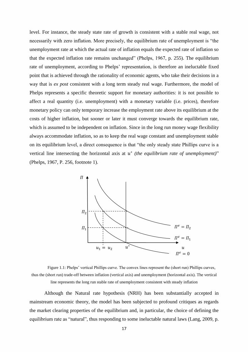
on its equilibrium level, a direct consequence is that “the only steady state Phillips curve is a

vertical line intersecting the horizontal axis at (the equilibrium rate of unemployment)”

(Phelps, 1967, P. 256, footnote 1).

Figure 1.1: Phelps’ vertical Phillips curve. The convex lines represent the (short run) Phillips curves,

thus the (short run) trade-off between inflation (vertical axis) and unemployment (horizontal axis). The vertical

line represents the long run stable rate of unemployment consistent with steady inflation

Although the Natural rate hypothesis (NRH) has been substantially accepted in

mainstream economic theory, the model has been subjected to profound critiques as regards

the market clearing properties of the equilibrium and, in particular, the choice of defining the

equilibrium rate as “natural”, thus responding to some ineluctable natural laws (Lang, 2009, p.

18

57; De Vincenti & Marchetti, 2005, p. 220). Friedman justified this choice by referring to the

well known Wicksellian natural rate of growth. The term “natural” is used to distinguish real

from monetary variables, the equilibrium rate of unemployment is natural because purely

dependent on real variables and because it characterizes a steady state growth path (Friedman

1968, 1977). Moreover, the term “natural” should not be interpreted, according to Friedman,

as immutable and independent from men, on the contrary “many of the market characteristics

that determine its level are man-made and policy-made” (Friedman 1968, p. 9).

Nevertheless, the ambiguity of the term “natural”, together with the non-clarified

Walrasian and non-Walrasian properties of the NRU, created the premises for the introduction

of a new equilibrium rate of unemployment, the Non Accelerating Inflation Rate of

Unemployment.

1.1.3. The Non-accelerating inflation rate of unemployment and its policy

implications

First introduced by Modigliani & Papademos (1975) as the Non inflationary rate of

unemployment (NIRU), the Non-accelerating inflation rate of unemployment (NAIRU) has

been rigorously developed by Layard et al (1991), which is still today among the most

influential academic works. This model keeps the general approach of the NRU, namely the

existence of a unique equilibrium rate of unemployment that is consistent with steady

inflation but independent on inflation itself. However, the introduction of monopolistic

competition in the labour market (unions are supposed to bargain a real wage which is higher

than the reservation wage of workers) makes the equilibrium between demand and supply

consistent with involuntary unemployment: to the extent that the NRU is associated to fully

voluntary unemployment, the NAIRU represents a special case in which the equilibrium real

wage, because it is higher than the marginal disutility of work, does not clear the market (De

Vincenti & Marchetti, 2005, p. 219).

In this framework there still exist some long/medium run endogenous mechanisms of

disequilibrium adjustment which are related to the relationship between inflation and

aggregate demand (Hein, 2005). When the rate of unemployment falls short of the NAIRU

and the effective real wage is higher than the equilibrium real wage, inflation accelerates in

order to keep up with nominal wage’s increases. Nevertheless, to the extent that the

acceleration of inflation reduces aggregate demand because of the real balance effect, the fall

19

in aggregate demand will push firms to adjust the quantity produced to the new level of

demand until the lower labour demand raises unemployment up to the NAIRU. The opposite

mechanism takes place if unemployment exceeds the NAIRU: in this case inflation

decelerates and real aggregate demand increases until the rate of unemployment falls back to

the steady inflation equilibrium.

According to NAIRU proponents, this new equilibrium rate of unemployment solves

the contradictions of the NRU as regards the term “natural” and its market clearing properties:

the NAIRU is an equilibrium characterized by monopolistic competition in the labour market

and it is consistent therefore with involuntary unemployment (the equilibrium wage rate is

higher than the marginal disutility of work). Unlike the NRU, it is not a market clearing

natural equilibrium; it is an equilibrium consistent with competing claims of employers and

employees. For instance, in this model unions bargain a non competitive real wage by

applying a mark-up over the reservation wage (hence, over the marginal disutility of work),

and firms set a non competitive price by applying a mark-up over the marginal productivity of

labour. The NAIRU is an equilibrium in prices expectations (such as the NRU) and in the

mark-ups: when the unemployment rate is equal to the NAIRU inflationary expectations turn

out to be met (the expected real wage is equal ex post to the actual real wage), hence the

mark-up applied ex ante by unions over the reservation wage is compatible ex post with the

mark-up applied by firms over the marginal product of labour. This property of mark-ups

compatibility explains why the NAIRU model is often referred to as the “battle of mark-ups”

(Layard et al, 1991). Moreover, the NAIRU model adds a “Keynesian flavour” to the original

Phelps/Friedman model: by introducing dynamic rigidities in the adjustment mechanism of

wages and prices, the NAIRU becomes a long term equilibrium rate which is not necessarily

met in the short and medium run, as long as aggregate demand fluctuations are not properly

anticipated by employers and employees. Consequently, countercyclical demand policies can

play a stabilizing role by accelerating the process of convergence towards the NAIRU.

Figure 1.3.1 reproduces the equilibrium rates of unemployment with perfectly

competitive markets (NRU) and with non-competitive markets (NAIRU). The Price Real

Wage (PRW) schedule represents the labour demand function in an economy characterized by

imperfect competition, in which firms set their price by applying a mark-up on the marginal

product of labour. The Bargained Real Wage (BRW) schedule represents the labour supply

function in an economy characterized by imperfect competition, in which unions bargain the

20

real wage by applying a mark-up on the reservation wage, which is equal to the marginal

disutility of work.

Figure 1.2: Employment and real wages in monopolistic competition with non competitive labour

markets (Source: De Vincenti & Marchetti, 2005)

Figure 1.2 allows capturing the differences between the NRU and the NAIRU

frameworks. The NRU represents a particular type of NAIRU that emerges when markets

work as if they were in perfect competition. If markets were perfectly competitive the

equilibrium real wage would be equal to the marginal disutility of work and to the marginal

productivity of labour, and the rate of employment would be equal therefore to .

Nevertheless, if the labour market is not perfectly competitive the equilibrium real wage lies

constantly above the marginal disutility of work and below the marginal product of labour

because of the mark-ups applied by unions and firms: the mark-up over the marginal

productivity of labour implies that the price set by firms is higher than the price that would be

set in a perfectly competitive environment, therefore the real wage is systematically below the

marginal product of labour for each level of employment. The mark-up over the reservation

wage (i.e. over the marginal disutility of work) implies that – given the expectations about

future price - the nominal wage bargained by unions is higher than the nominal wage that

each worker might be able to bargain individually in a perfect competition framework,

consequently the real wage is systematically above the marginal disutility of work for each

level of employment. The NAIRU is therefore an equilibrium that implies inefficiency in the

degree of utilization of aggregate resources (namely labour) and involuntary unemployment.

A

C

D

B

21

The NAIRU is an inefficient rate of unemployment because the real wage is lower than

the marginal productivity of labour; hence, it would be possible to hire a higher number of

workers who are willing to work by increasing total productivity and total output. The

measure of inefficiency is the inefficiency gap, which is the vertical distance between the

labour demand schedule (i.e. the marginal productivity of labour) and the Price Real Wage

(PRW) schedule, which is the labour demand function in the non competitive market. The

consequence of the positive inefficiency gap is the waste of productive resources, which is

measured by the difference between the level of employment at point A and the level of

employment at point C.

The NAIRU is also an equilibrium that is consistent with involuntary unemployment.

Indeed, if the labour market were perfectly competitive and the labour supply schedule

reflected the marginal disutility of work, unemployment would be necessarily voluntary, since

the unemployed would be those who are not willing to work at the equilibrium real wage

because of a larger disutility of work. Nevertheless, because of the monopolistic behaviour of

the representative union that applies a mark-up over the reservation wage, some of the

unemployed are willing to work at the equilibrium real wage, since their marginal disutility of

work is lower than the equilibrium real wage. The difference between the levels of

employment in point C and in point B of figure 1.2 represents the measure of involuntary

unemployment.

Therefore, the NAIRU represents a non market-clearing equilibrium rate of

unemployment that is consistent with the mark-ups that monopolistic firms and unions apply

to, respectively, the marginal productivity of labour and the marginal disutility of work. This

distributive conflict or “battle of mark-ups” implies an inefficient equilibrium characterized

by involuntary unemployment and waste of productive resources; moreover, it provides

different explanations of the unemployment/inflation dichotomy and different policy receipts

which are not fully equivalent (at least in the short/medium run) to standard explanations and

policy recommendations provided by theories of perfect competition, namely the theory of the

natural rate of unemployment. In the NRU framework, for instance, the equilibrium rate of

unemployment, the absence of any obstacle to perfect competition implies that the natural

rate of unemployment is a stable centre of gravity; therefore monetary policy is either useless

or counterproductive to the extent that it crowds out the automatic adjustment mechanisms. In

models based on imperfect competitions, on the other hand, a distinction has to be made

between the long run and the short/medium run (De Vincenti & Marchetti, 2005).

22

From a short/medium run perspective the NAIRU proponents reject the neoclassical

hypothesis of money neutrality. Although the NAIRU is as much an attractor as the NRU,

they are generally sceptical concerning the hypothesis of full substitutability of production

factors and flexibility of prices in the short/medium run. The existence of frictions in wage

and price adjustments is often introduced into these models in order to take into account the

possibility of a slow and sluggish adjustment to the long run equilibrium. Consequently,

countercyclical monetary policies are effective in the short/medium run in order to stabilize

more quickly the economy at the steady state. Suppose for example that degree of competition

in the labour market lowers: firms raise the price mark-up and the PRW schedule shifts

downwards. The equilibrium real wage falls and the NAIRU increases, therefore in absence of

monetary interventions the system would converge slowly to the new equilibrium through

inflationary pressures. If, however, the monetary authorities reduce the quantity of money

immediately after the shock, they will stabilize aggregate demand downwards at the higher

equilibrium rate of unemployment, avoiding a permanently higher inflation rate. Suppose now

that the PRW shifts upwards because of a higher degree of competition in the goods market.

In absence of monetary interventions the economy would undergo a transitory period of

disinflation and higher rates of unemployment with respect to the new equilibrium. Monetary

authority should thus increase the quantity of money in order to stabilize aggregate demand

upwards and reducing quickly the rate of unemployment. Hence, monetary policy is a

short/medium run effective tool to stabilize unemployment to the NAIRU, because these

rigidities would disappear. In the long run, however, money is still neutral as in the NRU

framework, since it cannot affect the equilibrium but only reduce the fluctuations around the

equilibrium. Only micro economic policies aimed at increasing the degree of competition by

liberalizing the goods and labour markets can push the NAIRU towards the NRU, which is

the unique market clearing equilibrium (De Vincenti & Marchetti, 2005).

1.1.4. NRU Vs NAIRU: differences and similarities

Although some characteristics of the NAIRU are not explicitly mentioned in the NRU

models of Friedman and Phelps, the debate is still open as regards whether the NRU and the

NAIRU are substantially different. The ambiguity of Friedman specification concerning the

NRU is probably at the roots of this controversy: is the NRU a voluntary rate of

unemployment grounded on a Walrasian system of general equilibrium equations or did

23

Friedman explicitly mentioned market imperfections as a source of involuntary

unemployment? According to Sawyer (1997) and De Vincenti & Marchetti (2005), the

NAIRU and the NRU must be considered as two distinct frameworks: the NRU is a market

clearing equilibrium that stands out from an analysis that assumes perfect competition, while

the NAIRU is an equilibrium rate of unemployment which is explicitly grounded on imperfect

competition and it is modelled as to achieve an equilibrium rate of unemployment that

displays both inefficiency and involuntary unemployment. The NAIRU introduces therefore

the distributive conflict as a possible source of inflation, which is not the case in the NRU

where inflation is only a monetary phenomenon related to a pressure of effective demand

above potential supply. Furthermore, assuming dynamic rigidities implies re-evaluating the

role of monetary policy as a stimulus to effective demand and employment, consistently with

the Keynesian framework: money is no longer neutral since it can stabilize the cycle around

the trend and avoid unemployment to increase above the NAIRU.

Nevertheless, according to Lang (2009) and Ball (2009) there are no substantial

differences in the two models, being the NRU and the NAIRU virtually synonyms (Ball,

2009, p. 4). Both the NRU and the NAIRU display time-reversibility and path-independence:

wherever the system starts from, it will sooner or later converge to an equilibrium rate of

unemployment which is to a larger extent exogenous. Asymptotic stability strongly relies on

assumptions that are common to both the NAIRU and the NRU, namely that the appropriate

equilibrium conditions include expectations being fulfilled and that the equilibrium is in the

long run supply-side determined. In particular, according to Sawyer (1997):

1) Both models assume, in the long run, the validity of the Say's law. Both the NRU and the

NAIRU are supply-side determined equilibrium rates of unemployment; shocks to

aggregate demand can only perturb the system but they do not change the equilibrium; As

a corollary, money is neutral in the long run.

2) The equilibrium is path-independent in both models. Small shocks or big recessions have

a different impact only in the short run, because in the long run unemployment will

converge back towards the NAIRU, without this latter being affected by the demand

shock. This conclusion is strictly related to the hypothesis that demand shocks do not

affect capital accumulation, since investments always accommodate savings, consistently

with the Say's law;

3) The NAIRU and the NRU are both treated as unique equilibria. Even when multiplicity of

equilibria is explicitly taken into account, “the estimation of the underlying equations and

24

the general discussion on the NAIRU proceed in a manner consistent with a unique

equilibrium” (Sawyer, 1997, p. 3);

4) The NAIRU and the NRU are both strong attractors, in the sense that both appear in

models built as to show asymptotic stability à la Lyapunov. If the system is perturbed in

the aftermath of a demand shock, unemployment will return back precisely to the

equilibrium, which is strictly exogenous with respect to demand;

5) Both the NRU and the NAIRU have “knife edge properties”, in the sense that any

disequilibrium level of unemployment is necessarily paid in terms of inflation or deflation.

There cannot be any other level of unemployment for which inflation is stable, the

NAIRU/NRU is the only unemployment level consistent with inflation stability.

Therefore, although the NRU and NAIRU frameworks are based on two different theories

of competition and have different policy implications in a short/medium run horizon, the long

run analysis of the economy is based on the same neoclassical “organizing concept”, namely a

supply-side determined and asymptotically stable centre of gravity. This neoclassical legacy,

however, raises important epistemological and theoretical concerns about the importance of

time and history, and the relevance of aggregate demand in the analysis of the long run.

1.1.5. Epistemological and theoretical remarks concerning the NAIRU and

the NRU

Neither the NRU nor the NAIRU can be directly observed in the real world, they both

represent theoretical concepts that can be at most estimated on the basis of some empirical

data and theoretical assumptions. The fact that they cannot be observed does not, however,

imply that they are of no use or interest for economic analysis. According to Sawyer (1997),

in social sciences many, if not all, concepts are not directly observable or measurable, some of

them do not even require to be observed and measured since they merely represent an

abstraction useful to implement a theoretic analysis, and both the NAIRU and the NRU

belong to this category. It could be of little interest to establish whether this equilibrium rate

of unemployment exists and which value it takes, but it could be probably of a bigger interest

to verify whether reality does actually conform to the predictions based on these models.

Friedman (1953), for example, endorses such view and goes even further arguing that it

25

cannot be of any importance the realism of a model, the most important property being its

predictive power.

Conformity to reality, however, does not necessarily imply the theoretical validity of

that concept. Even if reality did actually conform to the predictions of the NAIRU/NRU

framework, this would not imply that the equilibrium rate of unemployment observed is

indeed a NAIRU or a NRU: we cannot be content of verifying that reality conforms to the

predictions of the NRU model in order to validate the NRH. In the DSGE models, for

example, it is generally assumed that actual output naturally gravitates around its potential

because of the real balance effect (Palumbo, 2008). The fact that actual output does actually

display a cyclical tendency does not however imply that its average trend is necessarily a full-

employment and full-capacity output. The same applies for the NAIRU/NRU: the cyclical

fluctuation of the rate of unemployment around a given value does not imply that this average

trend is necessary a NAIRU or a NRU, nor does it imply that this average trend be necessarily

considered as a unique and absorbing equilibrium rate of unemployment. Indeed, in the

economic literature we can find different models of NAIRU, every one possessing some

different economic properties; hence, it would be difficult to decide which NAIRU is the

correct one only by ensuring that reality conforms to the predictions of a general NAIRU

model. To the extent that the NRU is considered as a particular NAIRU based on perfect

competition, it would be as much difficult to decide whether the equilibrium rate of

unemployment that conforms to reality is of a NAIRU or a NRU type. Conformity to reality

and theoretical consistency are therefore complementary, rather than substitutes.

There is another characteristic of the NAIRU and NRU frameworks that is highly

controversial: namely the assumption that demand always adjust to supply. This assumption is

not independent on the full rationality hypothesis: to the extent that genuine uncertainty is

ruled out and agents are assumed to rationally maximize a perfectly known environment, it is

reasonable to assume that demand shocks do not have lasting effect on the equilibrium as long

as agents keep on behaving as if the shock only consisted of a jump to a different initial

position. Therefore, in the NAIRU/NRU frameworks the equilibrium rate of unemployment is

purely supply-side determined, according to the implicit or explicit hypothesis that the

potential growth path is fundamentally exogenous with respect to demand shocks. Full

rationality, however, is not a sufficient condition to prove that the equilibrium is exogenous

and asymptotically stable. Two further assumptions are at least required: on one hand, that

there is always a level of demand able to absorb the entire production; on the other hand, that

26

disequilibrium positions systematically adjust towards the independently determined level of

supply consistent with full capacity and full employment.

The existence of a consistent demand for every level of supply is generally assumed

by Say's law or by the real balance effect. Say's law, consistently with the classical paradigm,

postulates that as long as money does not represent a commodity having a value per se but

only represents an instrument to purchase real commodities, any commodity which is

produced is necessarily sold and exchanged with other commodities. As a consequence, any

supply creates an equal demand. Say's law, which was at the core of the well-known

controversy between David Ricardo and Thomas Robert Malthus, had an extraordinary

influence in the Keynesian critique of the classical theory of value. In particular, according to

Ricardo effective demand could not have long lasting effects on aggregate supply because of

Say's law, while Malthus rejected such law and advocated the idea that capital accumulation

naturally reduces unproductive consumptions and, therefore, effective demand, causing a

systematic excess of supply over demand (Kurz, 1994). Although imprecise as regards the

causes of effective demand deficiencies, Malthus introduced the possibility that effective

demand might fall short of effective supply by determining a long lasting period of under-

utilization of capacity, a concept that Keynes developed in its General Theory by introducing

radical uncertainty and preference for liquidity as violating conditions of Say's law. Malthus

used for instance to define the Ricardian analysis in terms of “limiting principle”, according to

which the aggregate level of investments is limited by the level of aggregate savings

consistent with full-employment and full-capacity utilization. However, the contingent state

of the economy would depend on the “regulating principle”, according to which a discrepancy

between demand and supply might persist over a long period of time without necessarily

adjusting towards the full-capacity supply barrier. In other words, Say's law implicitly

postulates the asymptotic equality between the Malthusian “regulating” and “limiting”

principles.

The debate between Friedman and Keynes is to some extent the same between Ricardo

and Malthus. Indeed, Keynes did not argue specifically against the notion of a “natural rate”

of unemployment but rather against the stability properties of such equilibrium:

“Keynes could have readily agreed with Friedman on the definition of the “natural rate of

unemployment” (…) as corresponding to full employment (taking into account frictional and search

unemployment) but differed in the major respect as to whether there was a strong feedback mechanism

leading actual unemployment to the natural rate. Keynes would view the forces leading the actual rate

27

of unemployment towards the “natural rate” as weak, and the achievement of the “natural rate” would

require a high level of aggregate demand. In contrast, Friedman would view the adjustment of real

wages in the face of excess supply of labour as the mechanism by which the unemployment moved

rapidly to the “natural rate” (Sawyer, 1997, P. 4)

Full employment represents an upper bound which is theoretically unquestionable, but it

reflects neither an equilibrium nor an average state of rest: to the extent that production does

not automatically adjust to full-capacity supply in the aftermath of a demand shock, the new

equilibrium can be persistently below the full-employment and full capacity barrier.

Alternatively to Say's law, the real balance effect postulates the adjustment of demand

to supply through a wealth effect of inflation/deflation on consumptions demand: inflation

(deflation) reduces (increases) the real value of money and, thereby, the real demand of

goods. It is interesting to note that this mechanism works only under specific conditions. On

one hand, there is the implicit assumption that lower prices and falling prices are equivalent:

to the extent that the unemployment rate is above the NAIRU, prices are expected to fall and

demand to increase, which is controversial in a real economy where expectations matter and

investments are financially constrained (Sawyer, 1997). On the other hand, the effect of

inflation on the real interest rate is essentially neglected: the increase (fall) in prices is only

expected to decrease (increase) effective demand through a lower (higher) net wealth, ruling

out pro-cyclical effects on investments through a fall (increase) of the real interest rate.

Hence, the stability of the NAIRU implies that the real balance effect dominates the real debt

effect, which implies in turn a propensity to consume for the renters higher than the

propensity of investing out of retained profits for firms, which is unusual in a real economy

(Hein, 2005). Therefore, the asymptotic stability of the NRU/NAIRU strongly relies on a set

of controversial assumptions that are crucial to make the economic models consistent with

homeostasis and time-reversibility. To the extent that these assumptions are proved not to

hold, the whole model becomes extremely fragile and theoretically inconsistent. Hence,

conformity to reality is not a sufficient condition to validate these models, since “if those

models are on some relevant criteria judged to be unsound, then estimates and policy

conclusions derived are seemly unsound” (Sawyer, 1997, p. 2).

28

1.2. Path-dependency, supply-side time variance and hysteresis in the

mainstream approach

1.2.1. Time irreversibility and path-dependence: an empirical evidence

From an empirical point of view, the asymptotic stability property of the neoclassical

paradigm has proved not to hold with the main stylized facts of the last decades. After the oil

shocks and the deflationary policies of the 1980's, the unemployment rate in several European

countries rather than showing a convergence towards an independent and predetermined

NRU, as suggested by the theoretical models, displayed a growing trend that did not seem to

be only temporary (Ball et al, 1999; Ball, 2009). The same applies in several Latin American

countries in the late 40 years, where unemployment does not show any divergence-

convergence pattern (Ball et al, 2011). Cerra & Saxena (2008) analyse the impact of financial

and political crises in a set of 190 countries in the period 1970-2000 and show that when a

crisis has occurred, the output losses have been permanent. In particular, according to their

analysis, the negative effects of recessions are so persistent that only 1 percentage point of the

deepest outcome loss is regained by 10 years after the crises. That is, economic recovery is

simply a myth. As it appears in figure 1.3., when countries are hit by a recession we observe

two possible scenarios: either the level of output falls although the rate of growth does not

exhibit any long run damage, as it is the case for Korea and Chile, or the level of output and

the rate of growth permanently shift downwards, as it is the case of all other countries. More

recently, Ball (2014) analysed the consequences of the 2008 recession in Europe and had the

same results: in most European countries the recession has not been merely temporary,

potential output being permanently damaged. Figures 1.4 and 1.5 show indeed that in most

European countries actual GDP and GDP growth (the full lines) exhibit a permanent

downwards shift, therefore post-crises estimates of potential output growth (dashed lines) lie

below the pre-crises estimates (the dotted lines).

29

Figure 1.3: permanent output losses in the wake of strong meltdowns. The grey band represents the recession’s

duration, full lines represent the log of actual GDP (in the vertical axis) and dotted lines represent the linear

initial long run trend of GDP (in the vertical axis). Source: Cerra & Saxena, 2008

Not surprisingly, some econometric studies find that the equilibrium rate of

unemployment cannot be explained only by supply-side variables. Stockhammer & Sturn

(2012) find no significance of the labour market institutional variables in explaining NAIRU

estimates. Ball et al (1999) argue that labour market variables alone cannot explain the

dynamic trend in the equilibrium rate of unemployment. Jackman et al (1996) also argue that

labour market variables cannot explain the equilibrium rate of unemployment but merely

some persistence patterns. It seems, therefore, that standard NRU and the NAIRU frameworks

based on asymptotic stability cannot explain unemployment dynamics if they only focus on

labour market institutional variables, including unemployment subsidy duration, employment

protection and welfare policies. There is an important demand component in long run

equilibria that might explain a large part of unemployment’s variation and persistence.

30

Figure 1.4: examples of permanent output losses in the wage of the 2008’s Great Recession in a

sample of European countries. (Source: Ball, 2014)

31

Figure 1.5: examples of permanent output losses in the wage of the 2008’s Great Recession in a

sample of countries. (Source: Ball, 2014)

32

1.2.2. Supply side shocks, equilibrium multiplicity and hysteresis

During the 1970s and the 1980s, the sudden rise in unemployment appeared

fundamentally inconsistent with the long term vertical Phillips curve predicted by Friedman

(1968) and Phelps (1967). In his Nobel lecture, Friedman explained this non-vertical Phillips

curve as a transitory phase from a short run negatively sloped Phillips curve with zero

inflationary expectations to a long run vertical Phillips curve with expectations of positive

inflation, arguing that this transitory phase might last for a long time, “quinquennia or

decades” (Friedman, 1977). According to Friedman (1977), what accounted for the temporary

increase in unemployment despite the increase in inflation was the increasing price volatility

and uncertainty that prevented agents from extracting the good signals from the market by

creating disturbances in the process of adjustment of long run expectations. Hence, by

deciding to suddenly lower inflation through deflationary policies, monetary authorities could

not prevent unemployment to rise because of the higher volatility of prices and the sudden

reverse to a new steady inflation regime. The consequence is a medium run Phillips curve

being substantially negatively sloped, with lower inflation accompanied by higher

unemployment. In other words, the Friedman’s long run vertical Phillips curve is a very long

run equilibrium that holds as soon as the following conditions are eventually met: 1) the rate

of inflation is symmetrically volatile with respect to high or low levels of inflation; 2) relative

prices are free to adjust symmetrically with respect to inflation; 3) contracts can be freely

indexed to the new levels of inflation (Cross, 1984). The positively or negatively sloped

medium run Phillips curves are therefore only a transitory phase triggered by higher

uncertainty and prices volatility. As soon as inflation stabilizes and the three conditions are

met, unemployment will thus converge towards its “natural” level, consistently with the long

run vertical Phillips curve postulated by the (NRH). Although the deflationary policies

implemented in the 1980s in most of the European countries did actually make unemployment

increase, consistently with Friedman’s predictions about a transitory negatively sloped

Phillips curve, this growing trend did not seem to revert as the inflationary pressure fell, and

the unemployment rate permanently stabilized at a higher level. In order to explain the time

variance of the equilibrium rate of unemployment without rejecting the NAIRU framework,

we can distinguish three main theoretical approaches.

The first approach consisted of introducing the possibility of a multiplicity of

short/medium run equilibria characterized by path-dependence (Layard et al, 1991; Jackman

33

et al, 1996; Gordon, 1997, 1998; Richardson et al, 2000; Ball & Mankiw, 2002;). Persistence

of unemployment far from the long run steady state is explained by exogenous cost-push

shocks and by the structure of labour market institutions, namely the length and generosity of

unemployment benefits, the strength of employment protection legislation and the existence

of minimum wages that prevent unemployment to adjust towards the long run NAIRU. By

defining the short-run NAIRU as the level of unemployment consistent with steady inflation

in the current times, supply-side cost-push shocks and labour market rigidities might explain

the possibility to observe steady inflation and involuntary unemployment in the short/medium

run (Cross & Lang, 2011). Nevertheless, as soon as cost-push shocks cancel out, involuntary

unemployed must exert a downward pressure on real wages until unemployment adjusts to the

unique long-run NAIRU. Involuntary unemployment therefore can only be a transitory phase

characterized by real wage rigidity.

The second approach, which complements the first one, consisted of introducing the

possibility of exogenous structural changes in the “time-varying NAIRU” (Gordon, 1997,

1998; Richardson et al, 2000; Ball & Mankiw, 2002)1. To the extent that exogenous structural

changes, namely technological and labour market institutional shocks2, affect the long-run

NAIRU, the equilibrium can vary across time. In this framework, long run NAIRU’s

fluctuations are still explained by looking at the supply-side, demand plays no role on

equilibrium conditions in the long run. In other words, the time-varying NAIRU does not

tackle the stability and determinacy properties of the equilibrium in the wake of demand

shocks, but rather its uniqueness across time (Setterfield, 2008).

The third approach to unemployment persistence, that developed parallel to the

equilibrium multiplicity and the time-varying NAIRU theories, was proposed first by Phelps

(1972) and then formalized by Blanchard & Summers (1986) by referring to the concept of

hysteresis. In contrast to the long run vertical Phillips curve hypothesis that postulates the

independence of the equilibrium rate of unemployment from inflation, Phelps (1972) had

already introduced, on a purely theoretical ground, the possibility that a fall in the steady rate

of inflation might increase not only actual unemployment but also its equilibrium rate.

Generally speaking, the long run Phillips curve in Phelps (1972) is rather symmetric and

1 This approach is fully consistent and complementary with the equilibrium multiplicity approach. For instance,

models of time-varying NAIRU explain contemporarily short/medium run multiplicity by introducing cost-push

exogenous shocks, and long run time-variance by introducing exogenous structural changes. 2 Ball & Mankiw (2002) review a series of possible causes affecting the long run NAIRU, namely globalization,

job market institutions and productivity acceleration.

34

negatively sloped: a fall or increase in the unemployment rate, caused by, respectively, an

increase or fall in the rate of inflation, can permanently change some characteristics of the

labour market in a way consistent with, respectively, a permanent reduction or increase in the

NRU. Phelps' argument run as follows: when inflation decreases and workers experience a

temporary increase in the rate of unemployment, the new equilibrium rate of unemployment

that emerges when inflation stabilizes is not necessarily the same as before but will rather be

higher, since unemployment implies a loss of skills and productivity that permanently changes

the equilibrium conditions. Moreover, to the extent that employers perceive the unemployed

as less productive and not employable, it becomes harder for the unemployed to find a new

work position. A second mechanism that, according to Phelps, might imply a permanent shift

of the NRU is the change in the structure of real wages when a temporary variation of

employment leads to a permanent variation in the rate of unionization. These two

mechanisms, that Blanchard & Summers (1986) formalized later on, are at the roots of the

modern mainstream theory of hysteresis.

Although the term hysteresis came into a broader use in economics with Phelps (1972)

and Blanchard & Summers (1986), traces of a hysteretic reasoning in economics go back to

the classical economists. In particular, according to Marshall in its “Principles of Political

Economy”:

"if the normal production of a commodity increases and afterwards again diminishes to its old amount,

the demand price and supply price are not likely to return, as the pure theory suggests they will, to

their old positions for that amount" (Marshall, 1890, pp. 425-26, cited in Cross, 1993)

Nicholas Kaldor, John Maynard Keynes, Joseph Schumpter, James Tobin and Nicholas

Georgescu-Roegen also referred improperly to hysteresis to put forward the possibility that

changes in a given input variable have persistent effects on another output variable, without

however explicitly referring to the works of J.A. Ewing, who first introduced the concept of

hysteresis in Physics in the late 19th

century (Cross, 1993). Hysteresis is a term that was

coined by the physicist J.A Ewing, who discovered an interesting property of metals when

submitted to a demagnetizing and then re-magnetizing force: their field of force permanently

changes, inconsistently with the Maxwellian paradigm of homeostasis (Amable et al, 1993;

Lang, 2009). What Phelps (1972) and, in particular, Blanchard & Summers (1986) call

hysteresis is actually a generic form of path-dependence that implies an extreme instability of

the equilibrium rate of unemployment in the wake of demand shocks, without necessary

exhibiting the main dynamic properties of the original model of hysteresis. In particular,

35

under the influence of the seminal paper by Nelson & Plosser (1982), hysteresis has been

associated to the existence of a unit root in the wage-price spiral, which generates a

continuum of steady state rates of unemployment instead of a unique, asymptotically stable

long run NAIRU.

1.2.3. Hysteresis as unit-root persistence

1.2.3.1. Epistemological assumptions

The origins of the unit-root models of hysteresis are in the seminal paper by Nelson &

Plosser (1982), who analyzed the statistical properties of a set of time-series about

unemployment and output to conclude that non-stationary, random walk models explain real

trajectories better than standard stationary models. This empirical result was not neutral from

a theoretical point of view: if stationary model could allow representing growth and

fluctuations as mutually independent, random walk models are by definition non-stationary,

therefore they are not mean-reverting unless properly differentiated (see section 1.2.4).

Consequently, if real trajectories follow a random walk process, traditional models that

distinguish between a long run deterministic trend and short run stochastic deviations lose

their empirical relevance, since temporary shocks are no longer neutral on the equilibrium.

Based on their empirical results, Nelson & Plosser (1982) conclude about the necessity

to develop integrated models of business cycles and growth trends in which short run

stochastic fluctuations determine the long run trajectory. Blanchard & Summers (1986), who

introduce hysteresis as “the possibility that increases in unemployment have a direct impact

on the “natural” rate of unemployment” (ibid. p. 15) and then define it as “a very high

dependence of unemployment on past unemployment” (ibid. p. 17), clearly go in the direction

suggested by Nelson & Plosser (1982). By using hysteresis and path-dependence roughly as

synonyms, the authors argue that “a dynamic system is said to exhibit hysteresis if it has at

least one eigenvalue equal to zero (unity, if specified in discrete time)” (ibid. p. 17). NRU and

hysteresis are therefore represented as two different and, to some extent, opposed frameworks,

respectively a stationary/path-independent and a non-stationary/path-dependent one. In other

words, hysteresis is a form of path-dependence, based on the existence of a unit root, which

implies a radical violation of asymptotic stability and stationarity, the two main properties that

36

characterize the NRU framework3. The term hysteresis has been largely used in the wake of

Blanchard & Summers (1986) to define non-stationary processes that exhibit a unit root.

1.2.3.2. Theoretical models of hysteresis

According to Blanchard & Summers (1986), the sources of hysteresis in

unemployment are in the real wage bargaining process. In particular, long-term

unemployment is supposed to hamper real wages flexibility through virtually two main

channels, the insider-outsider conflict and human capital accumulation. According to the

insider-outsider theory (Lindbeck & Snower, 1986), to the extent that unions' members are the

employed, that is “the insiders”, and that they are able to organize in order to prevent the

outsiders from exerting a downward pressure on wages, changes in the rate of employment

have no impact on the equilibrium real wage. Consequently, an adverse transitory economic

shock that raises unemployment can imply a permanent shift in the labour supply schedule

instead of a downward pressure in the real wage, by making unemployment structural. A

different, but compatible, mechanism explaining a permanent shift in the labour supply

schedule relies on human capital deterioration. The intuition is that long-term unemployed,

because of their prolonged inactivity, lose their skills and their working abilities, and to the

extent that firms are reticent to employ them, early retirements and discouragement would

reduce the labour force and increase the rate of unemployment consistent with steady

inflation. Note that human capital deterioration is not necessary to explain the reluctance of

firm to hire long term unemployed as long as a “stigma” effect is on work (Lang, 2009): to the

extent that firms perceive long term unemployed as less productive by associating long term

unemployment to loss of skills and disaffection to work, long term unemployed would not be

hired independently of the real human capital deterioration. Furthermore, the “stigma effect”

also applies to the workers side by reducing their job search effort. When unemployment is

low, the unemployed are stigmatized because they are considered not to be actively searching

for a job, and social pressures push them to a higher job search effort. However, when

unemployment is higher and mass unemployment appears as an involuntary phenomenon, the

unemployed are less stigmatized and social pressures to increase the effort of job search are

3 Note that hysteresis, in this framework, does not only imply the existence of a unit root, but it implies also the

endogeneity of actual unemployment with respect to past realizations. For instance, also Gordon (1997) assumes

a random walk process for the natural rate of unemployment; nevertheless Gordon’s model is not a model of

hysteresis because erratic shocks are assumed to be exogenous and independent on unemployment.

37

lower. Hence, according to the “stigma effect” mechanism, long-term unemployment implies

a shift in the NAIRU because long term unemployed are perceived by firms as less productive

and because they do not actively search for a job. Unemployment hysteresis is therefore a

consequence of the real wage rigidity with respect to employment variations, because of

human capital deterioration, because of the “stigma” effect or because of workers resistance

to real wage cuts. As a consequence, even though unemployment increases the real wage does

not fall, and the level of unemployment that keeps the real wage (hence prices) constant, the

NAIRU, becomes higher.

However interesting from a theoretical perspective, the insider-outsider theory of

unemployment has been criticized for not being able to comply with the empirical evidence of

low and falling unionisation rates in most European countries (Visser, 2006). In other words,

there is no clear relationship between unionisation and unemployment hysteresis (Ball, 2009).

Furthermore, the model relies on the assumption that unions only seek to maximize the

insiders’ utility, irrespective of the outsiders, which is not necessarily the case for most

European countries where a large share of unions’ members are outside the employed

dependent labour force (Visser, 2006). A complementary argument concerning

unemployment hysteresis, which calls into question social norms’ rather than unions’ power,

focuses on the effect of fairness in wage bargain (Skott, 2004). Workers are assumed to

bargain money wages on the basis of what they consider a fair real and relative wage. Firms,

on their hand, know that if they accommodate the workers' demand, workers will be

productive, while if they offer a wage which is lower than the fair one, workers will organize

to reduce their overall productivity through shirking, striking, and so on. In order to obtain the

highest level of productivity, firms always accommodate workers request and pay the fair

wage. To the extent that the fair wage depends on previous real wage realizations, transitory

shocks might have permanent effects: if a sustained economic growth increases the fair real

wage, when unemployment suddenly raises because of a negative downturn firms keep on

paying the fair wage in order to obtain the highest level of productivity. Consequently, the

real wage does not fall and the level of unemployment consistent with real wage stability

becomes higher.

By focusing on capital stock adjustments, Blanchard & Summers (1986) argued that a

potential source of hysteresis might also depend on what they called the “physical capital

story” (ibid, p.27). To the extent that capital and labour are ex post not substitutable, a

negative shock affecting capital stock affects also overall employment. When the economy

38

recovers from the shock and demand increases again, the lower capital stock implies

inflationary pressures that slowdown and virtually neutralize the recovery. This theoretical

explanation of hysteresis relying on capital shortage, however, does not appear as plausible

from a neoclassical perspective to explain unemployment hysteresis. According to Blanchard

& Summers (1986) in the long-run capital and labour are perfectly substitutable; therefore, an

unexpected negative shock can cause unemployment to rise but in the long term, as firms can

shift from a capital intensive to a labour intensive technique, there is no reason to believe in a

capital stock constraint. Hence, to the extent that the real wage is flexible enough, the number

of jobs created by new investments will compensate the number of jobs destroyed by the

negative shock, and the NAIRU does not change. Consequently, for them, real wage rigidity

rather than capital shortage is at the roots of unemployment persistence (Layard et al, 1991).

There is, however, a growing literature that rejects the assumption of perfect

substitutability and underlines the crucial role of capital accumulation in determining both the

equilibrium and the instability of unemployment. Econometric estimates of the elasticity of

substitution provide a value which is closer to 0 rather than 1 (Rowthorn, 1999), suggesting

that capital and labour are not substitutable but rather complementary. To the extent that the

hypothesis of perfect substitutability of capital and labour is removed, capital shortage might

explain a large share of unemployment (Van de Klundert & Van Schaik, 1990; Rowthorn,

1999; Arestis et al, 2007). The capital shortage theory has important economic implications. It

can offer an important explanation of hysteresis by looking at the goods market rather than the

labour market; Furthermore, by introducing complementarity in capital and labour, the long-

term equilibrium rate of unemployment is no longer determined by the supply side only: it can

be demand-led and path dependent. There are, however, some drawbacks in the capital

shortage theory of hysteresis. According to Lang (2009), there is no reason to believe that in

the long run labour be still constrained by a lower level of capital, since a sustained recovery

accompanied by a higher expected demand should stimulate further investments and,

therefore, higher employment. Hence, it is not clear what should prevent unemployment to

regain the ex ante level when recovery takes over. In other words, it is not clear why a

transitory shock should necessarily have a permanent effect.

According to Arestis et al (2007), what might generate hysteresis in the wake of

capital shortage is the reaction of monetary authorities that target a steady inflation rate. The

argument runs as follows: suppose a negative transitory shock caused, for example, by the rise

in oil prices. This inflationary pressure exasperates the social conflict as regards who should

39

carry the costs, and prices increase even further. In order to avoid hyperinflation, governments

implement restrictive monetary policies, with negative consequences on capital accumulation

and employment. A possible recovery would thus trigger a raise in inflation that would be

hampered by a new restrictive monetary policy. Hence, an adverse transitory negative supply

shock might imply a permanent loss of productive capacity that is policy induced (Fontana &

Palacio-Vera, 2005). The two necessary conditions in order to have hysteresis in the wake of

supply shocks are therefore a monetary policy reacting to inflation gaps and an endogenous

mechanism of productive capacity adjustment in response to demand shocks.

Lavoie (2006) and Fontana & Passarella (2014) explain the endogeneity of productive

capacity by focusing on the Harrodian concept of natural rate of growth (Leon-Ledesma &

Thirlwall, 2002; Libanio, 2009). In particular, they argue that the natural rate of growth,

which depends on the rate of growth of labour productivity and the rate of growth of the

labour force, is endogenous to the actual rate of growth. Therefore, to the extent that a

transitory positive shock to aggregate demand fosters new investments that raise output and

labour productivity growth (Kaldor, 1957), the natural rate of growth will also increase.

Nevertheless, according to Lavoie (1996) and Cassetti (2006), hysteresis might also be a

consequence of adjusting the rate of capacity utilization rather than the rate of capital

accumulation. To the extent that firms produce by running productive capacity at the normal

rate, there might be hysteresis if what firms consider as normal depends on both historical

conventions and past realizations. According to Robinson (1956), for instance, entrepreneurs

tend to adapt their behaviour to subjective experience. In particular:

“Where fluctuations in output are expected and regarded as normal, the subjective normal-price may

be calculated upon the basis of an average or standard rate of output, rather than capacity (...) Profits

may exceed or fall short of the level on the basis of which the subjective normal prices were

conceived. Then experience gradually modifies the views of entrepreneurs about what level of profit is

obtainable, or what the average utilisation of plant is likely to be over its lifetime, and so reacts upon

subjective–normal prices for the future” (Robinson, 1956, cited in Lavoie, 1996, pp. 127-128)

Hence, if because of a negative supply shock the rate of capacity utilization falls, firms might

interpret this temporary change as a permanent change in market conditions and stabilize the

rate of capacity utilization at a lower normal rate. Besides norms and conventions, however,

the normal rate of capacity utilization might also depend on the existence of capital

indivisibilities, economies of scale and multiplicity of production techniques (Nikiforos,

2013). Since productive capacity is by a large amount indivisible, firms might produce at a

40

lower than normal rate of utilization when demand for their product is relatively low,

especially if a firm has different production techniques implying a different utilization of

fixed capital and different shifts. As a consequence, for a cost-minimizing firm, an increase in

market demand might lead to an increase of the desired rate of capacity utilization as long as

the returns to scale are increasing in the degree of utilization. In other words, the rate of

capacity utilisation of a firm does not fluctuate around a fixed and exogenous normal rate, it

rather fluctuates and stabilizes, under certain conditions, at different optimal or desired rates.

Therefore, a temporary deviation from the norm is likely to change the norm itself.

Even though the different theories of hysteresis do not necessarily converge towards

the same economic mechanisms (some relying on the wage bargaining process, some relying

on capital scrapping or capital accumulation and some relying on the choice of the optimal

degree of capacity utilization), most of these theories converge towards the same modelling

technique. By referring to Setterfield (1998) we might say that stating (or asserting) the

existence of hysteresis and providing a different theoretical explanation does not necessarily

imply a different way of modelling hysteresis. What we observe, on the contrary, is that these

different theories of hysteresis converged towards the unit/zero root approach.

1.2.3.3. Empirical models of unit-root persistence

The largest strand of the economic literature modelled hysteresis as a unit root process,

or as a system of linear differential equations with at least one zero eigenvalue, is the path

followed by (Blanchard & Summers, 1986; Van de Klundert & Van Schaik, 1990; Lavoie,

1996, 2006; Kapadia, 2005; Fontana & Palacio-Vera, 2005; Cassetti, 2006; Schoder, 2012;

Fontana & Passarella, 2014; Kienzler & Schmid, 2014).

Define the equilibrium as:

(1)

is a stochastic shock with . If <1, the unemployment time series is stationary

and will converge to the unique and stable equilibrium

(2)

41

If however =1, the unemployment time series is a random walk, that is a non stationary time

series with a unit root. In such a case, equation (1) will turn into

= + (3)

Equation (3) represents an example of hysteretic process: the realizations of depend on the

whole series of past shocks that affected the economy. In other words, although will, with

probability 1, revert sooner or later to , the economy might persistently fluctuate around

for an unpredictable time horizon.

The zero root approach lies on the same assumption than the unit root approach,

namely that hysteresis implies non stationarity. However, since the focus in no longer on a

single autoregressive process but on a system of linear differential equations, non stationarity

is contingent on the existence of at least one zero eigenvalue. To illustrate this approach we

refer to Lavoie (2006). By assuming that the rate of growth of potential output is a function of

the difference between real output and potential output:

(4)

And that real output growth is also a function of the difference between real output and

potential output:

(5)

Equations (4) and (5) can now be rewritten in matrix form:

(6)

The determinant of the Jacobian matrix is clearly null, since equations (4) and (5) are linearly

dependent. This implies that the homogeneous system, with the time derivatives equal to zero,

does not have a unique equilibrium but rather a continuum of equilibria. Furthermore, the

trace of the Jacobian matrix, that is the sum of the main diagonal, is negative: Tr(J) = .

According to the Routh-Hurwitz conditions, a negative trace implies that equilibria are stable:

if the system is perturbed from a given steady state, it will regain a different steady state. A

positive trace, on the other hand, would imply that the continuum of equilibria is fully

unstable: small perturbations imply a growing divergence from the steady state. If we

compute the characteristic roots of the matrix we get at least one zero eigenvalue:

42

The source of hysteresis lies on the existence of a zero eigenvalue in the system of

linear differential equations. According to the unit root approach, on the other hand, the

source of hysteresis lies in the existence of a unit root in the unemployment auto-regressive

process, which takes the form of a random walk. Since the most important difference between

the two approaches is the choice between difference or differential linear equations

(Setterfield, 1998), it is interesting to focus on the similarities in terms of dynamic properties.

First, unit root and zero root processes imply a full memory of the previous shocks. A random

walk is by definition a non-stationary process that keeps the memory of all past shocks, as

equation (3) clearly shows. In other words, the memory bank of the process is proportional

and “elephantine”: any shock, either small or big, will proportionally affect future equilibria.

A second common characteristic of these two approaches is “full reversibility”, which is

associated with their linear structure. In both approaches, although a stochastic transitory

shock implies a permanent change in the final equilibrium, cumulatively neutral shocks

always imply cumulatively neutral changes. Since stochastic shocks are by construction

cumulatively neutral, the effects on the equilibrium are cumulatively neutral as well, although

characterized by a strong persistence. The third characteristic is that linear models of

hysteresis are, if properly differentiated, mean reverting (De Peretti, 2007). For instance, if we

rearrange equation (1) by assuming =1we get

(7)

is mean reverting. In other words, although the unemployment rate does not converge to

a constant mean, unemployment variation is stationary around zero.

An alternative approach to unit root persistence characterizes hysteresis as a structural

change (Setterfield, 2008). By assuming a non-linear relationship between shocks and

equilibrium adjustments, a temporary shock might have a permanent effect by changing the

structure of the system of equations that determine the long run equilibrium. In particular,

based on the works of the Physicists J.A. Ewing and F. Preisach, Cross, (1993, 1994) and

Amable et al (1993) introduced the genuine model of hysteresis as an alternative to unit root

models in order to explain unemployment hysteresis. In this approach, hysteresis is no longer

characterized by linear persistence but rather by endogenous structural changes.

43

1.3. Alternative approaches to hysteresis: cumulative non neutrality,

discontinuous adjustments and structural change

1.3.1. Persistence Vs structural change

The random-walk approach suggested by Nelson & Plosser (1982) had a huge impact

not only on theories of hysteresis but, generally speaking, on growth theories, especially in the

Real Business Cycle (RBC) framework (Kydland & Prescott, 1982; King, Plosser & Rebelo,

1988; King & Rebelo, 2000). As long as transitory deviations affect the trend permanently, it

is no longer possible to analyse business cycles by distinguishing between deterministic

trends and stochastic fluctuations. By analysing the same time-series of Nelson & Plosser

(1982), Perron (1989) argued that a simple model of structural change could also explain that

same tendencies, without need to assume the existence of a unit root. Since then, several

econometric analyses have confirmed that models of structural change are also able to

perfectly fit with empirical data (Hansen, 2001). Papell et al (2000) analyzed the

unemployment time series of a set of OECD countries and could reject the unit-root

hypothesis for 10 out of 16 countries in favor of the alternative hypothesis of a single

structural break. Arestis & Mariscal (1999) analyze the unemployment time series in a set of

26 OECD countries and find one to two structural breaks in each of the time series. Hence,

they can reject the unit-root hypothesis for up to 22 out of 26 countries, in favor of a single or

double structural change.

Distinguishing between random walks and alternative linear or non-linear models

allows reaching radically different conclusions in terms of short run fluctuations and long run

tendencies. Amable et al (2004) show that the non-linear model of “genuine” hysteresis (see

section 1.3.3) can generate a non-stationary output that can be easily confused with a random

walk. However, if properly differentiated, the random walk is mean reverting, while the non-

linear model of “genuine” hysteresis is not (De Peretti, 2007). Consequently, empirical

analysis showing that aggregate time series exhibit unit roots are not sufficient to argue in

favour of modelling output and unemployment as random walks. Alternative theories of

hysteresis that focus on structural changes would equally fit with empirical data, providing

however a different characterization of the trend-cycle relationship, thus different economic

and policy implications.

44

1.3.2. Hysteresis as a theory of structural change

A different approach, which is more general than the unit root one, characterizes

hysteresis in terms of endogenous structural changes (Roed, 1997). Hysteresis implies the

violation of the standard path-independent and stable framework: there is hysteresis when

there is not convergence to an exogenously determined equilibrium rate. Hysteresis is

characterized in this framework by endogenous structural changes that affect the main

parameters of the economy and thereby the long run equilibrium. According to Roed, for

instance, hysteresis needs not to be found in the specific properties of some variables but

rather in the system of equations determining the equilibrium rate, in particular as regards the

exogenous and the endogenous variables. Whereas in the standard NRU/NAIRU models the

parameters can change only because of exogenous shocks, hysteresis implies that parameters

can also change endogenously, according to the contingent movements of the system outside

of the equilibrium. Generally speaking, suppose a function of this form (Roed, 1997):

(8)

f(.) is a fixed function, U is a vector of past realizations of u, x is a vector of exogenous

variables, X is a vector of past realizations of the exogenous variables x and y is the vector

that captures the exogenous structural changes. According to Roed (1997), the equilibrium is

path-independent and non-hysteretic if:

(9)

That is, if unemployment depends on exogenous variables and exogenous structural changes

only, it is time-independent and non-hysteretic. Hysteresis is defined as the violation of

equation (9), hence as the equilibrium dependence on past realizations of u and x that

generates endogenous structural changes.

The structural change approach to hysteresis appears to be more general than the

unit/zero root approach: if on one hand this characterization of hysteresis can include unit root

processes, it is also open to a broader spectrum of possible situations, including non-linear

models of hysteresis. Furthermore, the existence of endogenous structural changes might rule

out the hypothesis of a unique and stable long run exogenous equilibrium rate. In this sense it

might represent a “falsification” of the standard NAIRU model (Lang, 2009, p. 115).

However, this too broad definition includes any path-dependent dynamics, turning hysteresis

into a synonym of path-dependence.

45

According to Setterfield (1998), however, hysteresis is a special case of path-

dependence:

“hysteresis exists when the long-run or final value of a variable depends on the value of the variable in

the past, by virtue of the influence of this past value on the current alleged exogenous variables,

coefficients and structural equations which characterize the system that determines the variable” (ibid.

p. 284).

Hysteresis is not just a matter of short-run disequilibrium: it is a violation of the long run

homeostatic property of macro dynamic systems. Furthermore, hysteresis exists when “the

cumulative impact on (...) the long run outcome of a system of movements along a prior

disequilibrium adjustment path, is non zero” (ibid. p. 292), since it involves an “explicit

structural change in the system that is determining long run outcomes” (ibid. p. 294). This

definition of hysteresis as a disequilibrium adjustment process related to “cumulatively non

neutral changes” clearly separates hysteresis from generic forms of path-dependence and

multiplicity of equilibria. According to Setterfield (1998), hysteresis is a particular type of

path dependence that emerges from the reconsideration of the asymptotic stability properties

of the attractors. While systems with multiple equilibria generally imply the existence of a

continuum of equilibria - some of whom still possessing the property of stability - depending

on the initial position, hysteresis calls for a more radical uncertainty concerning not only the

initial position but also the specific adjustment path:

“A hysteretic system may actively create its own set of final outcomes in the course of its evolution as

a result of this structural change. (…) it may only be within our powers to identify these outcomes ex

post, after they have actually been established. They need not exist ex ante, independently of the actual

history of adjustments” (ibid, p. 294).

More precisely, in Setterfield (1998) hysteresis emerges consequently to “adjustment

asymmetries”. Let define

(10)

Let also assume that the variable X undertakes a cumulatively neutral change in the time

interval [1,n]:

(11)

According to Setterfield (1998), there is hysteresis as long as cumulatively neutral changes in

X imply cumulatively non-neutral changes in Z:

46

(12)

Hysteresis is triggered by a cumulatively non-neutral change of Z caused by a cumulatively

neutral change in X. From a mathematical point of view, cumulative non-neutrality is a

consequence of asymmetry and non-linearity of . Indeed, if Z were a linear function of X,

cumulatively neutral changes of X would necessarily imply cumulatively neutral changes in

Z. From an economic point of view, this “cumulative non neutrality” depends on structural

changes that happen to the system of equations determining Z when the variable X is

perturbed.

This characterization of hysteresis displays significant differences with respect to the

unit root approach. First, the unit root approach requires non-stationarity by definition, while

the “adjustment asymmetries” approach only requires asymmetric structural changes, which

are virtually consistent with both stationary and non-stationary processes. In other words, this

structural change approach does not necessarily require non-stationarity; it only requires non-

ergodicity, which is a property consistent with stationarity (Grazzini, 2012). Second, the unit

root approach only requires the knowledge of the starting point and the amplitude of the shock

in order to determine the arrival point. In the “adjustment asymmetries” approach, on the

other hand, uncertainty is not only related to the initial position and to the amplitude of the

shock, but also to the structure of the long run outcome: the same initial position can lead to

different and undetermined long run outcomes according to the amplitude and frequency of

structural changes. Consequently, it is not possible to predict ex ante the final equilibrium as

long as the set of information only includes the initial position (Setterfield, 1998, p. 293-294).

This approach differs also from the “endogenous structural change” one in terms of

lower generality: hysteresis is no longer a synonym but a special case of path-dependence.

Nevertheless, it gains in terms of generality with respect to the “genuine” hysteresis

framework (see section 1.3.3.): for instance, if “genuine” hysteresis implies adjustment

asymmetries, adjustment asymmetries do not necessarily imply “genuine” hysteresis. This

definition of hysteresis includes a broader set of models that might not display the properties

of “genuine” hysteresis, namely selective memory and remanence. Nevertheless,

characterizing hysteresis as an “endogenous structural change” that emerges from “adjustment

asymmetries” that bring about “cumulatively non-neutral changes” seems the most consistent

approach when thinking of business cycles as cumulatively neutral fluctuations. Next section

47

introduces the model of genuine hysteresis, which belongs to the larger family of models that

exhibit adjustment asymmetries and endogenous structural changes.

1.3.3. Sunk costs, discontinuous adjustments and hysteresis: an

endogenous structural change approach

J.A Ewing first coined the term hysteresis in the late 1881, when he noticed an

unexpected property of ferric metals that did not revert to their original position after a

complete cycle of magnetisation and demagnetisation. Indeed, at that time the dominant

paradigm in Physics was the homeostatic system of equations of Maxwell, which assumed the

return of the ferric metal to its previous state after the magnetising force had been removed

(Cross, 1993; Lang, 2009). J.A. Ewing conducted the experiment at the macro level. Half a

century later, the Hungarian physicist Preisach, who formalized the model of hysteresis,

explained the micro-mechanism conducing to hysteresis. According to Preisach (1935), ferric

metals are composed of micro elements named “hysterons”, or “hysteresis operators”, which

respond to magnetisation according to two distinct critical values: the hysteron is either “up”

or “down” according to whether the magnetising or demagnetising force is sufficiently high to

trespass the relative threshold value. The important feature of ferric metals is the fact of being

composed of multiple and heterogeneous micro particles, the hysterons, that respond

discontinuously to the external magnetisation force. In 1989, the Russian mathematicians

Krasnosel'skii and Pokrovskii, who were interested in generalizing this model to other

scientific fields other than physics, formalized the mathematical properties of the Preisach

model. Eventually, in 1991, the Ukrainian mathematician I. D. Mayergoyz developed an

intuitive graphical method to represent the dynamic properties of hysteresis.

Hysteresis is a macro behaviour that emerges from the aggregation of multiple and

heterogeneous elements, the hysterons. It has a micro (weak) and a macro (strong)

representation: weak hysteresis denotes the hysteretic behaviour of each hysteron; strong

hysteresis denotes the result of hysterons’ aggregation. To understand micro hysteresis it is

necessary to investigate the structure of the hysterons, in particular as regards the way they

respond to a magnetic shock. When a metal is subject to a magnetising force, the hysterons

either magnetise or they do not, according to the amplitude of this force with respect to a

couple of critical values: a lower critical value, say b, under which the hysteron is “down”; an

48

upper critical value, say a, over which the hysteron is “up”. The structure of each hysteron can

be represented by the “non-ideal relay”:

Figure 1.6: The non-ideal relay

The output is a binary variable equal to 0 (down) or 1 (up) on the basis of two switching

values, a and b, and the input shock. If the hysteron is “down” and the input shock is

sufficiently high to trespass the critical value a, the hysteron will switch to “up”. If the

hysteron is “up”, in order to switch to “down” the input shock must be sufficiently negative to

trespass b. If, however, the input shock is higher than b but lower than a, the hysteron will not

change its state: if it was “down” it will stay “down”, if it was “up” it will stay “up”.

Formally, if “O” stands for output and “I” stands for input, the set of possible outcomes is the

following one:

(13)

The input-output relationship is clearly non-linear, and it implies a discontinuous and

asymmetric adjustment of output to input changes. Suppose for instance that the output

variable at time t takes value 0 and the input variable is in between a and b, say on . If

suddenly the input variable increases above a, say on , the output will switch to 1, but if at

time t+1 the input variable comes back to , that is in between a and b, the output does not

switch back to 0. Note, however, that the cumulative impact can also happen to be null with

respect to the output variable, depending on the initial position. Suppose the initial output is 0

and the input variable is below b, say on . As soon as the input variable increases above a,

Output (O)

Input (I)

1

0

49

on , and then comes back to , the cumulatively neutral shock on input implies a

cumulatively neutral effect on output.

These examples illustrated the properties of weak hysteresis: the amplitude of the input

shock does not matter per se, since the memory bank of the process retains only the shocks

that are able to make the output variable switching from one state to the other. A small shock

that implies a switch from one state to the other will have longer lasting effects than a bigger

shock that does not imply a switch of the output variable. There is not necessary

proportionality between input shocks and output reactions. The three main properties of micro

hysteresis that arise from non-linear and discontinuous adjustments are the following ones

(Lang, 2009, p. 145):

1) The history of the system matters: the non-linear and discontinuous relationship

between input and output makes the present state dependent on the extreme values of

the past shocks.

2) There can be remanence if a cumulatively neutral input shock makes the output

switching from one state to the other. This possibility depends on the specific shock; a

cumulatively neutral input shock can imply a cumulatively neutral output shock.

3) Remanence does not depend necessarily on the amplitude of the shock, since there is

no proportionality between input and output.

Strong hysteresis emerges from the aggregation of the multiple and heterogeneous weakly

hysteretic behaviours, and can be represented graphically in the Mayergoiz’s half plane

diagram:

Figure 1.7: representation of the Mayergoiz’s half-plane diagram. The origin corresponds to the lowest a and b

thresholds.

b

a

a=b

U

D

Min[a] Min[b]

50

The diagram in figure 1.7 is defined only in the upper half plane, since the critical value a is

always, by definition, higher than the critical value b. Each point in the upper half plane

represents a specific hysteron. The “U” area includes the hysterons that are “up”, since

, while the “D” area includes the hysterons that are “down”, since . In order to show

the input-output dynamics we can start from figure 1.8. If the Input raises to , the U and D

areas change as follows:

Figure 1.8: representation of a positive shock in the Mayergoiz’s half-plane diagram. Positive shocks move on

the vertical axis. Full lines identify the current state of the system; dotted lines identify the history of the system

After the shock, some hysterons switch to “up” and the U area becomes larger. Suppose now

that the shock was only temporary, and that the Input reverts back to :

Figure 1.9: representation of a negative shock in the Mayergoiz’s half-plane diagram.

The U area is now smaller, although bigger than at the very beginning. For instance, after the

first shock some hysterons switched to “up” because , and when the input reverted at

the initial level, those hysterons did not revert back to down because still . Hence, a

b

a

a=b

U

D

Min[b] Min[a]

b

a

a=b

U

D

Min[a]

Min[b]

51

temporary shock left permanent traces. This property of genuine hysteresis according to

which temporary shocks can have permanent effects is called remanence. The difference with

respect to unit-root persistence, which also implies that temporary shocks have permanent

effects, is the non-linear reversibility of the process. Suppose a negative shock such that

followed by a positive shock such that :

Figure 1.10: representation of a cumulatively neutral shock in the Mayergoiz’s half-plane diagram.

The U area, which is the area below the full lines, is now bigger than the U area of figure 1.7,

even though shocks were cumulatively neutral. In other words, all these shocks left a

permanent trace that could not be erased just by reversing the process, hence just by applying

a series of cumulatively neutral shocks. Notice that remanence does not imply irreversibility:

the previous magnetic force can be potentially restored through a given sequence of shocks.

Nevertheless, what distinguishes remanence from “full reversibility” is the way the system

can restore the previous aggregate output: in unit root models, it is sufficient to trace back the

same sequence of shocks; in strong hysteresis, it is not sufficient to have cumulatively neutral

input shocks to have cumulatively neutral output shocks. However, some shocks can erase the

memory of previous shocks. Suppose a negative shock such that and then a

positive shock such that :

b

a

a=b

U

D

Min[b] Min[a]

52

Figure 1.11: representation of a series of shock that erase the memory of the system

Figure 1.11 shows the selective memory property of strong hysteresis: the shock

erases the memory of dominated shocks, namely to , that no longer determine

the aggregate output level. Indeed, the cumulative effect generated by the whole series of

shocks is equivalent to the cumulative effect generated by the

shorter series [ , the other shocks no longer provide information about the final state

of the system; this would have not been the case in absence of . Selective memory means

that only non-dominated shocks remain in the memory bank of the system, as opposed to unit

root processes that keep the whole series of past shocks in their memory bank. Furthermore,

the shock is able to restore the initial state of the system, since remanence does not

necessarily imply irreversibility, it only rules out linear reversibility through cumulatively

neutral shocks. This point can be better understood by looking at Ewing’s hysteresis loop in

figure 1.12:

b

a

a=b

U

D

= Min[b]

Min[a]

53

Figure 1.12: J.A. Ewing’s hysteresis loop

It is possible to reach any point on the vertical axis in both directions, although a different

input level is required. In other words, the points “A”, “D” and “G” represent different input

levels consistent with the same output: starting from A, if point B is reached, it is not possible

to reach the same output of A just by getting back to the same input level, since at that input

level the output will now be point C. In order to reach the initial output level it is necessary to

move to point D, which implies, however, a different input. Therefore, although the system is

not irreversible, it is not even linearly reversible. This is the main feature that distinguishes

remanence from persistence: remanence implies that cumulatively neutral sequences of input

shocks do not cancel out. The properties of strong hysteresis are similar to the properties of

weak hysteresis, with some additional remarks:

1) History still matters, but only as regards non-dominated.

2) There is remanence for virtually any fluctuation of the input variable, according to the

fact that firms are multiple and heterogeneous, and any cumulatively neutral shock

will potentially affect some firms and be neutral with respect to others.

3) Remanence depends on the amplitude of the shocks, in particular as regards their

quantitative effect: big shocks generally affect a larger share of micro-elements than

small shocks. The effect, however, is still not proportional because of the

heterogeneity in the threshold values.

The intuition behind the application of this model into economics is straightforward

(Dixit, 1989; Cross et al, 1998, 2008; Zoega et al, 2002): in many economic decisions, the

A

B C

D

E

G

F

Input

Output

54

different possibilities involved can be simplified in a dualistic choice (investing/ not investing,

hiring/not hiring). The final decision depends on the specific value that a given variable takes

with respect to some critical thresholds. Suppose a firm that faces the decision whether to

invest or not to invest in a new foreign market (Amable et al, 1994). This firm will invest if

expected returns exceed expected costs. Since sunk costs cannot be recovered if the

investment fails, the firm will require that expected returns be sufficiently high to fully

compensate the risk of net losses. However, if the firms decided to invest and actual returns

are lower than expected, it will make sure that the “exit” costs are lower than the costs of

staying before disinvesting and abandoning the market. Formally, the firm’s “entry” criterion

will be the following (Setterfield, 1998):

(14)

where R denotes total revenues, C the variable costs, K the sunk costs of entry and r the rate

of time preference. The “exit” criterion, on the other hand, will be:

(15)

The reason is quite intuitive: when the firm has to decide whether to enter in a new market or

not, its investment decision requires that the expected profits be higher than the value of the

fallback position, which is equal to 0 by assumption. If the firm already invested, in order to

exit the expected costs of staying (that do not include sunk costs, since they are paid once for

all) need not be just higher than 0 but need to be higher than the costs of abandoning the

market, which are equal to the “entry” costs (sunk costs).

Notice that, in order to have weak hysteresis, the existence of sunk costs, hence of two

different switching values, is a necessary and sufficient condition. In order to have strong

hysteresis two further assumptions are required: firms' multiplicity and heterogeneity. It can

be easily argued that different sectors exhibit different sunk costs. Furthermore, firms can

differ, within the same industry, in terms of managerial ability, financial constraints,

productive techniques and future expectations. The influence of “animal spirits” and radical

uncertainty on investment decisions is another important source of heterogeneity (Lang, 2009,

pp. 141-142). To the extent that firms are heterogeneous, they will have different expectations

concerning the future exchange rate and different critical thresholds. The non-ideal relay

diagram describes the investment behaviour of each firm:

55

Figure 1.13: the non-ideal relay diagram with expected exchange rate as the input variable and

investment as the output variable.

If expected profits are a function of the expected exchange rate, an inactive firm will decide to

enter in the market (I=1) if the expected exchange rate is above the critical value .

An incumbent firm, on the other hand, will decide to abandon the market (I=0) only if the

expected exchange rate is below the critical value , otherwise it would be better

off to stay in even though its actual profits are lower than expected. Hence, the number of

active firms in the foreign market will depend on expectations: if the expected exchange rate

increases, all inactive firms with will enter in the market; if the expected exchange

rate falls, only active firms with will exit from the market; all other firms, either active

or inactive, will not change their strategy as long as . The aggregation of firms’

discontinuous adjustments of capital stock in response to real exchange rate fluctuations will

generate strong hysteresis in aggregate capital stock fluctuations.

Empirical applications of this model are developed in Piscitelli et al (2000) on the Keynesian

consumption multiplier, in Cross et al (1998) on the relationship between real exchange rate

and unemployment and in De Peretti & Lang (2009) on Okun’s Law.

1.3.4. Genuine hysteresis Vs unit root: non linearity, selective memory and

remanence

There are strong theoretical and methodological differences between the two approaches to

hysteresis that are dominant in economic literature, namely the unit/zero root approach and

the genuine hysteresis approach.

Investment (I)

Expected exchange Rate (E)

1

0

f(-K = f(K

56

First, the unit/zero root models are dynamic models of linear differential equations that

identify hysteresis with the non-stationarity of the system. In particular, hysteresis is

contingent to the existence of a zero eigenvalue in linear systems of differential equations or a

unit root in difference equations. In the genuine hysteresis approach, on the other hand,

hysteresis emerges from the aggregation of multiple and heterogeneous hysteresis operators

that display a specific non-linear and discontinuous structure. However, it is not non-linearity

per se that generates remanence, but the specific discontinuous relationship between output

and input based on the existence of two distinct switching values. (Piscitelli et al, 2000)

Hysteresis is interpreted as a discontinuous and non-linear process of adjustment of output in

response to input shocks, in an economic environment characterized by multiplicity and

heterogeneity. The same cannot be said for unit root models, where hysteresis emerges from a

continuous and partial adjustment of output in an economic environment characterized by

homogeneity.

Although the difference can appear to be purely methodological, the economic implications

are often at odds. Unit root models of unemployment hysteresis implicitly assume that

hysteresis is a very special case: since the unemployment rate is by definition bounded

between 0 and 1, unemployment time series cannot be represented by random walks, which

are stochastic processes characterized by a virtually infinite variance. Moreover, when the

assumption of a unit root is tested against the alternative hypothesis of structural change,

standard econometric tests fail to reject the null hypothesis of stationarity (Arestis & Mariscal,

1999; Papell et al, 2000). Therefore, if unemployment hysteresis means the existence of a unit

root, the hysteresis hypothesis can be systematically rejected. To overcome such a limitation,

the assumption of a unit root is often relaxed and the sum of the lagged variables is no longer

constrained to be equal, but just close to 1. In this case, however, hysteresis would be

associated with short run persistence or equilibrium multiplicity, consistently with a long term

asymptotically stable equilibrium (Layard et al, 1991). Genuine hysteresis, on the contrary,

implies the explicit reconsideration of asymptotic stability of the attractors: when

discontinuous adjustment of heterogeneous agents takes place at the micro level, it is no

longer possible to identify a unique and stable macroeconomic equilibrium, since transitory

shocks might generate permanent effects, hence remanence. Consequently, hysteresis does

not emerge as a special case but rather as a structural characteristic of environments

characterized by heterogeneity and discontinuity. Furthermore, strong hysteresis is perfectly

57

consistent with both stationary and non-stationary time-series (Amable et al, 2004), and it can

explain a larger set of empirical observations with respect to strictly non-stationary models.

Second, random walks are stochastic processes that keep in their memory bank all past

shocks, whatever their amplitude and duration, as it clearly appears from equation (3).The

effect of input shocks on output is linear and proportional. Genuine hysteresis, on the other

hand, is characterized by a selective and erasable memory (Cross, 1994). Moreover, although

at a macro level some proportional effects can be found, these proportionality is only

“quantitative”, in the sense that a bigger shock is likely to imply the switch of a higher

number of firms with respect to a small shock, but it is not linear and it depends on the

sequence of past shocks. The property of selective memory has also important implications on

the reversibility of the process. Since unit root processes keep the whole sequence of the

previous shocks in the memory bank permanently, these processes display strict

irreversibility, even though cumulatively neutral shocks perfectly cancel out in a fully

reversible way (Amable et al, 1995). Genuine hysteresis, on the other hand, is characterized

by remanence, which has different implications with respect to either persistence or unit root

instability. Although remanence implies that “transitory shocks have permanent effects”,

these permanent effects do not cancel out just by reverting the process but they are not even

irreversible: “many subsequent time paths are possible for different sequences of shocks,

including a return to the original steady-state unemployment level. (…) There are costs

involved in the restoration of the status quo ante, but not irreversibility” (Cross, 1993B, p.

307). For these reasons, it would be more appropriate to speak about persistence, rather than

hysteresis, when dealing with unit/root models (Amable et al, 1994).

Asymptotic stability, unit root instability and remanence represent radically different macro-

dynamic frameworks that are not necessarily compatible each other. In particular, while the

unit- and zero- root approaches are consistent with long run asymptotic stability (hysteresis

being confined to the existence, in the short to medium run, of a unit- or zero-root), failing to

reject the NRH, genuine hysteresis is definitely incompatible with a long run natural rate of

unemployment. Genuine hysteresis is the opposite of the NRU, its falsifying hypothesis

(Lang, 2009, p. 109).

58

1.3.5. Policy implications and concluding remarks

According to the neoclassical theory, the long run is naturally characterized by a

balanced growth path that is exogenous with respect to effective demand. Monetary policy

can at most stabilize the cycle around its long run trend but it cannot modify the trend. Even

though introducing the possibility that temporary shocks might have permanent effects

implies, to a smaller or larger extent, the reconsideration of the NRH, the degree of rejection

of the mainstream asymptotically stable framework can be consistently different. According

to Ball & Mankiw (2002) and Ball (2009) hysteresis does not invalidate the classical NRU

framework but rather integrates it: to the extent that the NRU is made endogenous, the model

still holds and gains in terms of empirical consistency:

“Allowing for hysteresis can greatly change our explanations for unemployment movements and our

prescriptions for monetary policy. However, I don’t view hysteresis as a radical departure from mainstream

economic theory. It is not a rejection of Friedman’s model, but a generalization of it. We expand the set of

factors that cause the U* term (..) to change over time: these factors include movements in actual unemployment

as well as supply-side variables.” (Ball, 2009, p. 8)

To state that the NRH can be consistent with the hysteresis hypothesis, however, is

tantamount to confining hysteresis to a short run departure from the long run asymptotic

stability assumption. In other words, to the extent that hysteresis represents a special case of

an otherwise asymptotically stable long run, the dichotomy short-run/long-run still holds: in

the short run the economy might exhibit hysteresis, but in the long run the NRH cannot be

rejected. If, however, the hysteresis hypothesis is supposed to hold in a long run horizon, the

NRH will not hold any longer. Indeed, to the extent that the long run NRU/NAIRU is a weak

attractor or even an attractee, most of its operational and conceptual power would be

definitely lost, and by losing all its predictive power the NRU/NAIRU would be no longer an

interesting reference concept to analyse macroeconomic dynamics (Sawyer, 1997; Stanley,

2002; Palumbo, 2008). Questioning the stability of the equilibrium implies therefore

questioning the validity of the concept of equilibrium as an analytical tool. In Miroshima's

words:

“If economists successfully devise a correct general equilibrium model, even if it can be proved to possess an

equilibrium solution, should it lack the institutional backing to realize an equilibrium solution, than that

equilibrium solution will amount to no more than a utopian state of affairs, which bears no relation whatsoever to

the real economy” (Miroshima, “the good and bad uses of mathematics”, quoted in Kirman, 1992)

59

Since the “natural rate hypothesis” requires a relatively stable equilibrium and implies

monetary policy neutrality, hysteresis must lead to a rejection of the NRH as long as it implies

a large equilibrium instability and monetary policy non neutrality.

According to Ball et al (2011), for instance, monetary policy explains a large share of

unemployment, especially in the aftermath of recessions. Starting from the empirical evidence

that unemployment raised and stabilized upwards in some countries, while it returned back to

the initial level in others, they find a positive correlation between real interest rate and

unemployment: strong and sudden reductions of the real interest rate were associated with

falling rates of unemployment; sluggish real interest rates with higher and stable

unemployment rates. Hence, full employment stability would require a discretionary and

asymmetric monetary policy: if inflation decelerates, central banks should suddenly lower the

interest rates in order to prevent unemployment to become structural. When on the other hand

inflation increases, the interest rate should be kept relatively low in order to allow a structural

fall in the NAIRU before stabilizing inflation again. The opposite behaviour, consisting of

increasing the interest rate in response to small increases of inflation and not lowering the

interest rate when inflation decelerate, would rather hamper recoveries and structuralize

cyclical unemployment. According to Schettkat & Sun (2009), for instance, German

unemployment persistence in the last four decades can be attributed to an asymmetric

monetary policy of the Bundesbank: when the economy was supposedly overheating, the

Bundesbank immediately raised the interest rate in order to prevent an increase of inflation.

When, however, the economy was slowing down it kept real interest rates relatively higher by

raising the NAIRU. The authors blame the excessive emphasis on price stability and, in

particular, the systematic incapacity to correctly estimate the “output gap”. If potential output

is assumed to be always, on average, equal to actual output, and consequently potential output

is estimated as the weighted mean (or as a smoothed series) of the business cycle, the risk of

under- or over-estimating potential output sharply increases, since any recession or any boom

will be soon considered, on average, as structural. Therefore, underestimating potential output

leads to restrictive monetary policies to the extent that the lower output is considered to be

structurally lower.

60

Figure 1.14: Actual Vs potential output. The consequences of estimation biases.

Suppose the central bank is only interested in price stability and sets the interest rate

according to the estimated output gap, which is the difference between actual output and

(estimated) potential output: when the output gap is positive because actual output lies above

potential output, unemployment lies below the NAIRU and the central bank will increase the

interest rate in order to prevent an increase of inflation; when, on the other hand, the output

gap is negative because actual output lies below potential output, unemployment lies above

the NAIRU and the central bank reduces the interest rate in order to prevent a deceleration of

inflation. If the central bank assumes that actual output naturally gravitates around potential

output and at time estimates potential output as the average trend of real output, it might

interpret a negative output gap as positive output gap and increase the interest rate in order to

stabilize the economy on the improperly estimated long run trend. The consequence is a pro-

cyclical monetary policy that turns cyclical unemployment into structural.

Therefore, introducing hysteresis in unemployment implies reconsidering the role of

countercyclical demand policies, which do not merely stabilize demand around an

independent supply but they rather determine the long run trajectory of the economy.

Moreover, if hysteresis is a structural property of economies characterized by heterogeneous

and discontinuous adjustment behaviours - rather than a special case of unit root persistence -

the whole validity of the mainstream framework, as well as the policy prescriptions based on

this framework, are called into question. Chapter 2 will show, for instance, that introducing

genuine hysteresis in a “new consensus” framework radically changes the policy implications

of the model. Namely, demand shocks might imply a permanent loss of productive capacity

according to the amplitude of the shock and the reaction of the central bank. Furthermore,

GDP

Time

Actual Potential

Output trend

Estimated

Potential

Output trend

61

monetary and fiscal policies become a fundamental tool to set the economy around a range of

endogenous long run steady states instead of merely stabilizing demand around a unique (or a

predictable multiplicity of) exogenous long run trend. Hence, genuine hysteresis implies a full

reconsideration of the NRH and its policy neutrality implications, it definitely rules out any

“Natural Rate Hypothesis”.

62

2. Discontinuous entry and exit decisions. Long run non-neutrality of demand policies

2.1. Introduction

Section 2 of chapter 1 concentrated on recent developments in macroeconomic theory as

regards how path-dependency and hysteresis have been introduced in standard

macroeconomic analysis based on equilibria that are allegedly natural. We can distinguish

three different approaches to make the NRU/NAIRU model consistent with empirical

evidence of raising unemployment in most European countries, especially in the 1980’s. A

first approach refers to the assumption of a high persistence in the process of disequilibrium

adjustment that might generate a multiplicity of short- to medium- run NAIRUs because of

cost-push shocks and developed rigidities in the labour market triggered by, for example,

welfare institutions and employment regulation (Layard et al, 1991; Nickell et al, 1996;

Gordon, 1997, 1998; Richardson et al, 2000; Ball & Mankiw, 2002). By defining the short-

run NAIRU as the level of unemployment consistent with stable inflation in the current

period, the unemployment rate might temporarily fluctuate around a higher or lower

equilibrium although it must, sooner or later, revert to the unique, long run NAIRU (Cross &

Lang, 2011). A second approach focused on the possibility of supply-side structural changes

characterizing the NAIRU as a time-varying equilibrium (Gordon, 1997, 1998; Richardson et

al, 2000; Ball & Mankiw, 2002). In this framework, the NAIRU is still an asymptotically

stable equilibrium that can vary because of supply side shocks, namely technological

development, openness to trade and financial liberalization among others. The endogenous

relationship between demand and supply is, however, still rejected (or at least not discussed).

While these two approaches are consistent with the standard theory of a long run stable

NAIRU, the third one explains raising unemployment by assuming a radical violation of the

NRH. In particular, it is assumed that long-term unemployment deteriorates the human capital

of workers, who lose the capability to exert a downward pressure on real wages. When this

happens, the NAIRU completely loses its attractive force and fully adjusts to real

unemployment variations: rather than observing real unemployment adjusting to the

63

equilibrium we would observe the equilibrium adjusting to current unemployment. The

unemployment rate dynamics would consequently be suitable represented by a random walk.

The hysteresis hypothesis has largely influenced the macroeconomic debate. To the extent that

unemployment exhibits hysteresis, the fundamental neoclassical conclusion of the vertical

Phillips curve and the consequent money neutrality is rejected; consequently, forecasts based

on the short-run unemployment-inflation trade-off lose their predictive power.

The new mainstream macroeconomic paradigm that has been rapidly developing in the last

two decades (Clarida et al, 1999, 2000; Allsopp & Vines, 2000; Taylor, 2000; Mc Callum &

Nelson, 2000; McCallum, 2001; Woodford, 2001, 2003), often defined as the “new

neoclassical synthesis” or “new consensus in monetary macroeconomics” (NCM) (Fontana &

Palacio-Vera, 2005; Lavoie, 2006), seems to have only partially been affected by this debate.

In the “new consensus” view, the analysis of business cycles does not focus any longer on the

labour market even though it is mostly based on the same theoretical assumptions than the

NRU/NAIRU models. In particular, the dichotomy between actual and natural unemployment

has been replaced by the dichotomy between actual and natural output (Clarida et al, 1999).

Based on this assumption, the short-run unemployment-inflation trade-off has been also

replaced by a short-run output-inflation trade-off, and the standard expectations augmented

Phillips curve substituted by a similar price rule in which the output gap, which is the

difference between actual and natural output, replaces the unemployment gap, which is the

difference between actual and natural unemployment or, in alternative words, the difference

between the actual rate of capacity utilization and the non accelerating inflation rate of

capacity utilization (NAIRCU) (Gordon, 1998; Nahuis, 2003).

The real novelty of this framework seems to be the relevant role played by monetary policy in

stabilizing short run fluctuations. In the NAIRU model, for instance, the stability of the

equilibrium was assumed a priori relying on a simple real balance effect (see section 1.1.5.).

Nevertheless, by assuming the existence of rigidities in price setting that prevent actual output

to adjust to natural (or potential) output, the equilibrium stability is no longer guaranteed, and

the interest rate becomes the relevant fine-tuning variable to stabilize output fluctuations

around potential output . The role of the central bank in these models is to target the

Wicksell’s natural rate of interest, which is the rate of interest that guarantees the adjustment

of real to natural output, by setting a higher-than-natural rate when inflation accelerates and a

lower-than-natural rate when inflation decelerates. By following a simple inflation target,

monetary authorities could thus stabilize positive and negative fluctuations by setting the

64

proper interest rate according to the signal received by the market, respectively acceleration or

deceleration of inflation.

The strength of this framework is twofold. On one hand it allows to overcome the problem of

unemployment hysteresis by simply ignoring the labour market, in order to concentrate on the

capacity utilization-inflation trade-off and the role of monetary policy in ensuring at the same

time inflation stability and full capacity utilization.

From this point of view, the NCM represents a step forward with respect to the NRU and

NAIRU frameworks. For instance, the assumption of price rigidities is consistent with the

disequilibrium persistence and multiplicity of equilibria approach to hysteresis. Moreover, to

the extent that supply shocks can affect the output-inflation trade-off, persistent cost-push

shocks might generate a multiplicity of short run output equilibria that are different from the

long run natural output. The stabilizing role that monetary policy plays in these models

represents at the same time the recognition that the long run equilibrium is unstable and that

monetary policies are fundamental to stabilize the economy (Ball et al, 2011) and, on the

other hand, an immunization of the model with respect to hysteresis by assuming that

monetary policy alone is able to stabilize the economy, provided that the central bank

succeeds in correctly estimating the natural rate of interest and targeting a fixed and steady

rate of inflation. Therefore, the “new consensus” framework seems to provide an answer to

the hysteresis hypothesis by introducing monetary policy as a stabilizing device, and suggests

interpreting persistent fluctuations as either caused by an inefficient central bank that chooses

the wrong monetary rule (Clarida et al, 2000) or by exogenous structural changes, consistently

with the time-varying NAIRU approach. For instance, natural/potential output in these models

seems to be strictly independent from real output. Clarida et al (1999) and Woodford (2001),

by modelling potential output as a stationary process independent on output gap, clearly

separate growth and business cycles. In McCallum & Nelson (2000), potential output is a

function of a technology shock term and import prices, independently on output gap. Taylor

(2000) is vaguer on this point. On one hand he argues that potential output evolves according

to a classical Solow model augmented with endogenous technology, suggesting a form of

endogeneity in potential output evolution. Nevertheless, it clearly distinguishes economic

growth and economic fluctuations in two distinct chapters: while growth depends on

endogenous technology growth, economic fluctuations are explained by price rigidities and

monetary policy reactions, and there are no explicit links between business cycles and

65

technological growth. Hence, even though growth is assumed to be endogenous to demand

fluctuations, it is actually treated in the model as if it was exogenous.

Latest contributions to the “new consensus” framework tried to formally reconcile the

standard three equations model with the hysteresis hypothesis (Kapadia, 2005; Fontana &

Palacio-Vera, 2005; Lavoie, 2006; Kienzler & Schmid, 2014) by adding a fourth equation to

the model that defines an endogenous process (equivalent to the unit root process) of potential

output adjustment to real output variations. In particular, potential output (potential output

growth) is modeled as a linear function of past potential output (past potential output growth)

and past real output (past real output growth), according to the following linear

characterization (Hargreaves-Heap, 1980):

With 0 < < 1. Note that this characterization of hysteresis amounts to a quasi-unit-root

model: by setting the dynamic process of potential output adjustment becomes a unit

root process.

When equation (1) is introduced into the model, the system exhibits a zero root, and the

policy implications suddenly change. Supply-side negative shocks generate policy-induced

recessions (Fontana & Palacio-Vera, 2005; Lavoie, 2006): to the extent that the central bank

targets a fixed rate of inflation, a cost-push shock implies a monetary restrictive policy that

affects output and thereby potential output, the new equilibrium being characterized by steady

inflation but lower output. The same applies for supply-side shocks to potential output

(Kapadia, 2005; Lavoie, 2006): a transitory but persistent negative shock to potential output

(i.e. a technological shock) would raise the output gap and generate inflationary pressures,

that the central bank puts out by increasing the interest rate and adjusting output downwards.

The new equilibrium will be characterized again by steady inflation and lower output.

The same does not apply, however, in case of demand shocks (Lavoie, 2006) or

monetary policy shocks (Kienzler & Schmid, 2014): a temporary shock that raises or lowers

current output respectively above or below potential output can be perfectly neutralized by a

standard monetary policy rule without any consequence of potential output. In this case, for

instance, the temporary shock would initially imply a deviation of output from potential

output and, through equation (1), a dynamic movement of potential output itself. However,

the reaction by the monetary authority would imply an equal force of opposite sign that would

66

eventually imply the same dynamic process but in the opposite direction. As a consequence,

the economy would only temporary deviate from the initial equilibrium but then return back

to the original level of potential output. In other words, the equilibrium is eventually

characterized by global stability4. Introducing a unit/zero root in “new consensus” models

highlights therefore the importance of distinguishing between demand and supply side shocks

when a central bank targets a fixed rate of inflation. For instance, in case of demand shocks,

targeting inflation stability turns out to be a successful policy. In case of supply side shocks,

however, the emphasis on price stability would create policy induced recessions that persist in

the long run, unless a positive supply side shock of same amplitude brings the economy back

to the original equilibrium, consistently with the “full reversibility” property of unit root

models (see section 1.2.3.3.).

Chapter 2 develops a standard “new consensus” model with “genuine” hysteresis. Instead

of modelling potential output adjustments as a unit root process, it is assumed that a variety of

heterogeneous firms with different sunk costs, different expectations and different market

demand elasticity adjust discontinuously capital stock to expected profits variations. Each

firm can decide whether to enter/stay in the market and produce with 1 unit of capital, or

exit/not to enter in the market and have 0 units of capital. Since the investment decision is

made under fundamental uncertainty (Keynes, 1921; Knigth, 1921) and implies sunk costs

(Dixit, 1989), potential new firms enter in the market only if expected profits fully

compensate sunk costs; incumbent firms exit from the market if expected losses are higher

than sunk costs. If expected profits or losses are respectively lower or higher than sunk costs,

firms do not invest nor scrap their capital stock and just wait for more information (see

section 1.3.3.). By introducing this non-linear and discontinuous adjustment in firms

investment decisions, economic and policy conclusions radically change. In “new consensus

monetary” models with genuine hysteresis, for instance, the distinction between supply and

demand shocks becomes less relevant to policy decisions, since both types of shocks would

imply a shift in the final equilibrium. This is one of the main differences with respect to

unit/zero root models of hysteresis: in “new consensus” models with zero root persistence the

effects of transitory demand shocks cancel out in the long run equilibrium; in the “new

consensus” model with genuine hysteresis, demand shocks leave a permanent scarce in long

4 Palacio-Vera (2009) shows that by introducing a non-linearity in the price equation, temporary demand shocks

may have permanent effects, despite potential output dynamics are modeled via equation (1). Nevertheless, this

chapter considers NCM models with a linear accelerationnist Phillips curve and a hysteretic potential output

equation.

67

run output. In this framework, counter-cyclical monetary policies are no longer able to target

fixed output equilibria even though shocks are merely transitory and cumulatively neutral,

since equilibrium is fully endogenous and hysteretic. Discretionary monetary and fiscal

policies become crucial not only to smooth aggregate fluctuations but also to determine the

long run equilibrium of the economy, which is fully endogenous.

2.2. A “new consensus” monetary model with genuine hysteresis

2.2.1. The standard “new consensus” model

Consider a simplified standard New-Consensus model characterized by the three well-

known fundamental equations (Allsopp & Vines, 2000; Taylor, 2000; Lavoie, 2006):

Equation (2) represents the New-Keynesian IS curve, where represents a structural

disturbance that captures the autonomous demand side components, including government

expenditure, r represents the real interest rate, β a fixed parameter, g represents the output

gap, which is the difference between actual and potential output, and a white noise

stochastic shock responding to the following dynamic with = 05.

Potential output is defined in this model as the level of output consistent with a steady state

rate of inflation, in other words potential output represents the inflation barrier: when the

output gap is positive inflation accelerates, when the output gap is negative inflation

decelerates. This characterization of the output gap is explicit in equation (3), where

represents the rate of growth of inflation, a fixed parameter and a white noise stochastic

shock6. Equation (4) represents the central bank’s monetary policy rule, which is supposed to

replace the neoclassical theory of loanable funds, represented by the old LM curve, with a

theory of endogenous money in which the central bank cannot directly control the stock of

5 might represent either a stochastic demand shock or a fiscal policy shock. In the remainder of the chapter it

will be treated as a fiscal policy shock. 6 This characterization of the accelerationist Phillips curve implies simple backward looking expectations. For an

overview of different inflation rules with forward-looking expectations refer to Kapadia (2005)

68

money but can fix an interest rate according to a “reaction function” (Lavoie, 2006);

represents the Wicksellian “natural” real rate of interest, the inflation rate targeted by the

central bank, and represent fixed parameters and a white noise stochastic shock 7

.

2.2.2. Potential output and “genuine” hysteresis

Implicit to the standard new-consensus model is the idea that potential output is

substantially independent on aggregate demand and real output fluctuations (Fontana &

Palacio Vera, 2002; Lavoie, 2006). In other words, there is a “hidden equation” (Lavoie,

2006) that tells:

(6)

This equation does not necessarily imply that potential output is constant. Indeed, potential

output can be a time-varying variable as long as supply side shocks change the structural

conditions of the equilibrium (Gordon, 1998; Nahuis, 2003). Equation (6) implies that

although potential output is not time-independent, it is fundamentally demand-independent

since it is not affected by real output fluctuations, and can be treated as fundamentally unique

and globally stable provided that supply side shocks are ruled out by assumption or they are

assumed to be exogenous8. Consequently, temporary demand shocks cannot have long lasting

effects on the equilibrium conditions: in the long run real output converges towards potential

output because of aggregate supply stability and because of monetary policy based

mechanisms of disequilibrium adjustment (Clarida et al, 1999; 2000; Taylor, 2000; Allsopp &

Vines, 2000).

In particular, demand adjusts to supply through equations (3) and (4). According to

equation (3) a positive (negative) output gap implies an increasing (decreasing) inflation. To

the extent that the central bank is able to correctly estimate the “natural” rate of interest,

according to equation (4) the positive (negative) gap between actual inflation and targeted

7 The values of the parameters used during the simulations are provided in Appendix 1

8 It can be argued that standard New Consensus models do no aim at explaining growth but rather business cycle

fluctuations, and therefore they assume potential output stability only for simplicity. According to Taylor (2000),

for instance, potential output is obtained through a Solow model augmented with endogenous technological

change. However, the decision to clearly distinguish the long run growth behavior from a short run cyclical

behavior must necessarily rely on the hypothesis of substantial independence of the growth path from business

cycle fluctuations. Clarida et al (2000), for instance, clearly specify potential output as a AR(1) process: potential

output fluctuations are therefore explained through stationary and stochastic exogenous shocks, independently

from business cycle fluctuations. In other words, even though potential output is assumed to be theoretically

endogenous, it is actually treated as if it were exogenous.

69

inflation will trigger a raise (fall) of the interest rate up to the “natural” rate, which is the rate

of interest that equalizes aggregate investments and aggregate savings, hence real output and

potential output. Consequently, the economy will stabilize again along with a steady and

targeted inflation rate, a “natural” interest rate and a zero output gap. In this model, the

assumption of potential output stability is relaxed. In particular, firms’ potential output is

defined as the level of output consistent with a “normal” utilization of the productive capacity

installed, where by “normal” rate of capacity utilization it is generally meant the rate of

capacity utilization that implies the minimum cost for firms (Kurz, 1986; Nikiforos, 2013). It

is widely held, however, that firms tend to keep idle capacity in order to be able to face

unexpected peaks of demand and not losing market shares with respect to actual and potential

competitors. In other words, idle capacity can be on one hand a deterrent for new entrants and

on the other hand a competitive strategy (Lavoie, 1996; Palumbo & Trezzini, 2003).

Therefore, the “desired” rate of capacity utilization, which can be considered as the optimum

target for firms, is not necessarily cost minimizing and it does not necessarily represent an

“inflation barrier”. Since potential output is generally meant to be the maximum level of

output achievable without triggering pressures on inflation, the “desired” rate of capacity

utilization cannot be considered as a measure of potential output, while the “normal” rate of

capacity utilization can. For the sake of simplicity, we assume that normal and desired rates

coincide, and that the “normal” rate of capacity utilization is stable because of the stabilizing

role of prices: firms reduce (increase) prices when utilization is below (above) the “normal”

rate and expand (reduce) their market demand until the “normal” rate of capacity utilization is

reached, consistently with equation (3). We also assume for productive capacity a Leontief

production function, with scarce capital and constant full-capacity output to capital ratio equal

to 1 (A = 1) for simplicity. In economic terms, this hypothesis implies that production is a

function of capital stock only, consistently with the empirical findings of Rowthorn (1999):

(7)

Consistently with the standard models of “genuine” hysteresis (Piscitelli et al, 2000;

De Peretti & Lang, 2009; Cross et al, 2012) there is full capital indivisibility, consequently

firms’ investment decisions come down to a binary choice: either entering in the market with

a stock of capital equal to or exit from the market by scrapping their capital stock. Since

investment decisions are taken in a radically uncertain environment (Keynes, 1921) and they

imply sunk costs that cannot be recovered after the investment is made (Dixit, 1989), they

70

display a non-linear and discontinuous dynamic. In particular, new entrants wait for aggregate

demand to be higher than a certain investment threshold, say a, in order to invest and install a

capital stock equal to Incumbent firms, on the other hand, wait for aggregate expected

demand to be lower than a disinvestment threshold, say b, before scrapping the capital stock

and exit from the market. By using the output gap relative to potential output as a proxy for

aggregate demand, it is possible to represent investment decisions as in figure 2.1:

Figure 2.1: The non-ideal relay

If the output gap is above a, a new firm will found convenient to install a productive capacity

equal to and entering in the market, while an incumbent firm will just decide to stay in the

market. If the output gap is below b, an incumbent firm will find convenient to scrap

productive capacity and exit from the market, while a new potential entrant will just wait for

better times before entering in the market and investing. If however the output gap is in

between a and b, the incumbent firm will not find convenient to exit and a new potential

entrant will not find convenient to enter in the market. In other words, in between a and b

there is a “zone of inaction” that leads both potential new entrants and incumbent firms not to

change their strategy and wait for new information before taking a decision that implies

unrecoverable costs. The decision of a firm to enter or exit from the market is a path-

dependent decision:

(8)

71

The selective memory property of “genuine” hysteresis arises from the existence of this “zone

of inaction” in which incumbent firms do not exit and potential new entrants do not enter.

Starting from this zone, a temporary shock that is able to induce incumbent firms to exit or

potential new firms to enter will leave permanent traces on these firms: the incumbent firms

that decided to exit because of a temporary negative shock will not enter again when the

shock is over, and potential new entrants that decided to enter because of a temporary positive

shock will not decide to quit the market when the shock is over. A temporary shock, either

positive or negative, will leave permanent traces only if it is able to induce some potential

new entrants to permanently enter in the market or incumbent firms to permanently exit, while

it will leave no traces if it is not able to induce any firm to quit their zone of inaction.

For the sake of simplicity, both a and b are exogenous and constant over time, a

common assumption in standard models of genuine hysteresis (Piscitelli et al, 2000; Amable

et al, 2004; De Peretti & Lang, 2009). Consistently with standard models of genuine

hysteresis, firms are heterogeneous with respect to these switching values. It is reasonable for

instance to suppose that different economic sectors have different sunk costs according to the

specific characteristics of the markets. Furthermore, within the same sector and the same

market, firms can have a different demand and different expectations concerning how demand

will evolve in the future, hence a different propensity to take risk and invest. For instance,

firms observe the same aggregate demand shock (aggregate output gap) and on this basis they

form expectations concerning how their own market demand will evolve in next periods. For

example, some industries might not benefit at all from a little and positive aggregate demand

shock to the extent that the higher demand would be addressed to other industries; therefore,

they will need a bigger positive aggregate demand shock in order to have a little positive

increase in own market demand. The same applies for small negative aggregate demand

shocks: some industries will lose a consistent amount of demand as a consequence of the

downturn while some others will be only partially affected. The effect on individual output for

each firm depends on the different sensitivity to aggregate demand shocks, and it is different

for each firm as long as each firm (or industry) has a specific market demand elasticity to

aggregate demand shocks. Animal spirits will also affect the relative position of the switching

values and the way firms respond to aggregate demand shocks. To the extent that a firm is

particularly optimistic, a small positive increase in aggregate demand will be sufficient to

enter in the market since it will be interpreted as a sign of a long lasting growth period. At the

same time, optimistic firms will also interpret a downturn as merely temporary and will not

72

consequently scrap productive capacity. A pessimistic firm, on the other hand, will more

rapidly disinvest when demand falls and will wait for a higher demand before entering in the

market. Hence, an optimistic firm will have a relatively lower a and a relatively lower b with

respect to a pessimistic firm, since positive demand shocks will be interpreted as a sign of a

boom and negative demand shocks as temporary downturns.

The threshold values will be different for each firm if there is a unique input but

different elasticities of market demand with respect to aggregate demand variations, different

expectations concerning aggregate demand evolution and different sunk costs. Because of

heterogeneous sunk costs, heterogeneous expectations and heterogeneous elasticities of

individual demand with respect to aggregate demand variations, aggregate potential output

cannot be represented as a representative firm’s behavioral equation but rather as the

aggregation of heterogeneous firms taking independent decisions. Differently from the

standard “new consensus” model that assumes a unique representative firm, aggregate

potential output is the sum of heterogeneous firms’ potential output:

(9)

Next section shows the simulations of a standard “new consensus” model in which firms’

decision to increase or to scrap productive capacity depend on equation (8), consistently with

the “genuine” hysteresis paradigm. Differently from standard models of “genuine” hysteresis,

however, the input is no longer exogenous since it depends on equations (2) to (5). The aim of

the simulations is to compare the emerging results in terms of monetary and fiscal policy

effectiveness with standard NC models (Clarida et al, 2000; McCallum, 2001, Woodford,

2001, 2003) and NC models augmented with linear hysteresis (Kapadia, 2005; Fontana &

Palacio-Vera, 2005; Lavoie, 2006; Kienzler & Schmid, 2014; Fontana & Passarella, 2014).

2.3. Productive capacity adjustments: structural change Vs temporary

persistence

Simulations are performed in the multi-agent simulation environment .

There are 100000 firms having the same full-capacity output to capital ratio (A = 1) and the

same rate of “normal” utilization, , but different switching values according to a

73

uniform distribution9. We simulate different monetary policy scenarios consisting of different

weights put on output stability in the central bank’s reaction function, using the same random-

seed in all scenarios in order to isolate the monetary policy effect, and fixed monetary policy

coefficients but different random seeds in order to isolate the effect of the initial position.

Eventually, results are compared with those emerging from a standard New-Consensus model

with constant potential output and a linear hysteresis-augmented “new consensus” model

(Lavoie, 2006; Fontana & Passarella, 2014).

2.3.1. Permanent effects of temporary shocks and long run non neutrality

of economic policies

Figure 2.2 shows the impact of a temporary negative shock to with different

random-seeds.

Figure 2.2: Output dynamics with different random seeds

The hysteresis effect of a temporary shock is substantially different across simulations

depending on the starting point: different random-seeds imply different starting points, hence

different share of firms starting on their “inaction zone” and changing their strategy in the

wake of the shock. The same shock, whatever its amplitude, might have different effects on

final output according to the sequence of past shocks. Furthermore, the final equilibrium is

fully undetermined: instead of stabilizing along multiple predictable steady states, the system

can stabilize in a continuum of possible equilibria that cannot be predicted unless the initial

9 The specific random distribution does not affect the results and properties of the model (Piscitelli et al, 2000)

74

position of each firm that reacts to the shock is common knowledge. In most cases the

negative shock is sufficiently high to prevent a full recovery and the economy permanently

stabilize downwards. The reason is that following the negative shock some firms exit from the

market and consequently depreciate the overall productive capacity. Since both the output gap

and inflation fall, the central bank lowers the interest rate in order to boost demand and

stabilize the output around its (lower) potential. The final outcome is a permanently lower

output along with steady inflation and “normal” utilization of (a lower) capacity. These

scenarios are consistent with the capital shortage explanation of unemployment hysteresis

(Van de Klundert & Van Schaik, 1990; Arestis et al, 2007 and references therein): the

existence of sunk costs and the consequent discontinuity of investment decisions might

explain why, despite the recovery, productive capacity does not revert to the initial level, a

critical remark that has often been raised to capital shortage theories blamed for not being able

to provide a theoretical explanation of hysteresis (Blanchard & Summers, 1986; Lang, 2009).

Figure 4, however, also shows some apparently counterintuitive results. In some cases, for

instance, the economy stabilizes upwards along with a higher output despite the negative

shock. The reason is that the negative shock does not generate an important wave of exit;

therefore, when the central bank lowers the interest rate, the recovery is sufficiently strong to

induce new firms to enter in the market and increase the overall productive capacity. As a

result, when the economy stabilizes along with steady inflation and “normal” capacity

utilization, the overall productive capacity is permanently higher.

The final outcome depends on both the amplitude of the shock and the monetary

policy reaction of the central bank, which affects the capability of the economy to absorb the

initial shock and prevent large waves of firms’ exit. Figure 2.3 shows the impact of the same

shock, starting from the same starting point (i.e. same random seed)10

, under different

monetary regimes: the central bank can either caring about price stability only ( = 0) or

alternatively put a positive weight on output stability ( > 0).

10

Figure 5 shows the results of the simulations with the same random-seed. Indeed, results are consistent and

robust whatever the random seed chosen.

75

Figure 2.3: Permanent effects of temporary shocks with different monetary policy responses (different value

of ).

The same positive shock to has a different impact on final output according to the different

weight put on output stability by the central bank: the hysteresis effect is more consistent in

cases of slow reaction by the central bank, since aggregate demand falls sufficiently to induce

some firms to permanently exit from the market and stabilize output downwards. Monetary

policy has therefore a long run non neutral effect to the extent that it does not only affect the

shape of the business cycle but also the final equilibrium, especially in cases of asymmetric

reaction: stability-oriented in case of positive shocks and disinflation-oriented in case of

negative shocks (Schettkat & Sun, 2009). The same applies for fiscal policy: to the extent that

the central bank does not neutralize immediately a negative fiscal shock through a lower

interest rate, the effect on output of a restrictive fiscal policy can be negative both in the short

and in the long run

.

76

2.3.2. Policy effectiveness in linear hysteresis-augmented “new consensus”

models

In standard “new consensus” models, as long as potential output is kept constant by

assumption, a positive or negative output gap can only trigger a change in inflation,

consequently fiscal policies are always inflationary and monetary policies always stabilizing,

unless the zero lower bound is reached and positive fiscal policies become necessary to

stabilize the economy (Snowdon & Vane, 2005). Lavoie (2006) and Fontana & Passarella

(2014) show that this conclusion must be rejected in case of a permanent demand shock if we

assume that potential output is a linear function of both past potential output and current

output according to equation (10), which is a simple rearrangement of equation (1):

(10)

With 0 < < 1. A positive shock to fiscal policy that is not immediately neutralized by the

central bank through a higher real interest rate would lead to a permanent increase in real

output, as long as potential output adjusts upwards through equation (10), the output gap goes

back to 0 and inflation stabilizes back to the targeted rate.

We simulate the model by Lavoie (2006) assuming proportionately higher parameters with

respect to Fontana & Passarella (2014), in order to accelerate the process of convergence, and

assuming two different scenarios: the first scenario implies a permanent shock to which is

not neutralized by the central bank, while the second scenario implies a temporary shock

to , still not neutralized by the central bank11

. Eventually we compare the results with a

standard “new consensus” model that assumes equation (6) instead.

11

In the New Consensus models, the central bank neutralizes demand shocks through the natural rate of interest.

Since the exogenous and stochastic shock is, by assumption and by construction, a non-anticipated (fiscal

policy) shock, it does not affect the natural rate of interest. A permanent exogenous shock to is therefore

interpretable either as a non anticipated long lasting shock or as a correctly anticipated but not neutralized shock.

For the same reasons, a temporary shock to must be interpreted either as a non anticipated temporary shock or

as an anticipated structural shock that is neutralized through the natural rate of interest (in this case the central

bank will identify the permanent stochastic shock as a increase in the structural disturbance ).

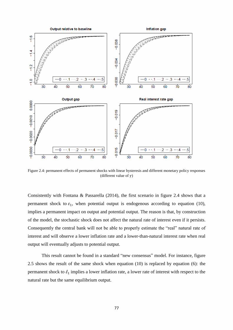
77

Figure 2.4: permanent effects of permanent shocks with linear hysteresis and different monetary policy responses

(different value of )

Consistently with Fontana & Passarella (2014), the first scenario in figure 2.4 shows that a

permanent shock to , when potential output is endogenous according to equation (10),

implies a permanent impact on output and potential output. The reason is that, by construction

of the model, the stochastic shock does not affect the natural rate of interest even if it persists.

Consequently the central bank will not be able to properly estimate the “real” natural rate of

interest and will observe a lower inflation rate and a lower-than-natural interest rate when real

output will eventually adjusts to potential output.

This result cannot be found in a standard “new consensus” model. For instance, figure

2.5 shows the result of the same shock when equation (10) is replaced by equation (6): the

permanent shock to implies a lower inflation rate, a lower rate of interest with respect to the

natural rate but the same equilibrium output.

78

Figure 2.5: Temporary effects of permanent shocks with asymptotic stability of potential output and different

monetary policy responses (different value of )

In this case, even though the current interest rate is different from the improperly estimated

natural rate and inflation is lower than the targeted rate, potential output will not vary at all

(again, by construction). The same does not apply, however, if we simulate a temporary shock

to . Figure 2.6 shows that although potential output is endogenous according to equation

(10), as long as the shock is only temporary there is no permanent effect on real output: the

negative initial shock implies an upwards adjustment of potential output, as soon as the

positive shock fades out potential output readjusts downwards up to the initial equilibrium. A

temporary negative shock is not able to change the structure of the economy as long as the

central bank, sooner or later, neutralizes it through a lower “natural” rate of interest or to the

extent that it fades out automatically. This result, which is also shown in Kienzler & Schmid

(2014) and analytically proved in Lavoie (2006), is perfectly explainable by the linear nature

of equation (10) and refers to the so-called “super-reversibility” property of linear models of

hysteresis: a sequence of positive and negative shocks of same amplitude imply a sequence of

positive and negative linear movements of output that are mutually offsetting.

79

Figure 2.6: Temporary effects of temporary shocks with linear hysteresis and different monetary policy

responses (different value of )

In particular, the negative initial shock is offset by the subsequent positive shock

implied by the central bank’s monetary reaction, namely the fall in the interest rate as a

consequence of falling inflation. The long run behavior of the system is consequently

equivalent to the long run behavior of standard “new consensus” models that assumes

equation (6): the real output goes back to the original level as soon as the temporary shock is

over (figure 2.7).

80

Figure 2.7: Temporary effects of temporary shocks with asymptotic stability of potential output and different

monetary policy responses (different value of )

Hence, fiscal and monetary policies have a long run effect on real output when

potential output is a linear and increasing function of the output gap only if the central bank is

willing to accept a rate of inflation different from the target. If we assume instead

that and that the central bank rigorously tracks the targeted rate of inflation,

positive or negative shocks (including fiscal policy shocks) can only affect the business cycle

but they cannot affect the long run equilibrium. This result can also be obtained by assuming

that equation (10) is a random walk by setting , according to the Blanchard & Summers

(1986) definition of hysteresis.

81

Figure 2.8: Temporary effects of temporary shocks with unit root hysteresis and different monetary policy

responses (different value of )

As shown in figure 2.8, by introducing a unit root in equation (10) we obtain the same

conclusions that would be obtained by setting . The reason is that in standard models of

unit root persistence, unemployment hysteresis implies that inflation stabilizes at a higher or

lower level when respectively unemployment stabilizes at a lower or higher level. In the “new

consensus” model, however, the reaction function of the central bank explicitly rules out this

possibility, since a rate of inflation higher or lower than the targeted level implies a higher or

lower rate of interest that adjusts output and potential output to the long run equilibrium. In

other words, the monetary rule of the central bank prevents that the economy might stabilize

at steady rates of inflation different than the targeted one and, thereby, that the economy

might exhibit long run effects because of temporary demand shocks. It is the central bank

behavioral function that explains why linear models of “hysteresis” cannot ultimately account

for the persistence of the effect (on output) beyond the cause that generated it (the exogenous

demand shock), i.e. hysteresis, in “new consensus” models.

82

2.4. Economic policy implications of “genuine” hysteresis and concluding

remarks

According to the paradigm of asymptotic stability, upon which the standard “new

consensus” model is built, the system has no long run memory of past shocks: to the extent

that the central bank adopts the optimal monetary policy rule (Taylor, 1996; Clarida et al,

1999; 2000; McCallum, 2001; Woodford, 2001, 2003) recessions or booms can only have

temporary effects until the system stabilizes back around its unique and asymptotically stable

equilibrium, which is the NAIRCU. Discretionary fiscal policies are in this framework seen as

destabilizing or at least as useless (Taylor, 2000B).

Introducing hysteresis through a linear function like equation (10) does not change

substantially the economic policy conclusions: as long as demand shocks are only temporary

and not systematic, introducing linear hysteresis will only affect the short run equilibrium and

the speed of convergence towards the unique long run steady state. Indeed, to the extent that

the central bank is committed to price and output stability, the optimal monetary policy rule is

still effective in stabilizing the economy, demand shocks and fiscal policies can be perfectly

neutralized. This conclusion is valid also by modelling equation (10) as a random walk,

consistently with the new-Keynesian literature of hysteresis (Blanchard & Summers, 1986;

Ball et al, 1999; Ball, 2009), unless a discontinuity is introduced via the price equation

(Palacio-Vera, 2009). In this case, even though potential output adjusts linearly to aggregate

demand, temporary demand shocks might have permanent effects on the long-run trend.

According to the “genuine” hysteresis-augmented “new consensus” model developed

in this chapter, hysteresis is a more general paradigm consistent with both stationary and non-

stationary trends (Amable et al, 2004). For instance, the effect of negative or positive shocks,

whatever their amplitude, always depends on the relative position of firms with respect to

their “inaction zone” and can consequently result in either temporary or permanent changes in

the contingent equilibrium. Remanence, for instance, implies that the amplitude of a shock is

not a sufficient information to determine whether there will be hysteresis or not: the history of

the system, that is the sequence of past shocks, is also an important source of information in

order to determine how the economy will respond to future shocks. In particular, temporary

demand shocks have permanent effects if the system is caught in a moment of relative

fragility, when most firms are within their “inaction zone”. Furthermore, remanence implies

that long lasting or deep recessions are likely to trigger a permanent loss of potential output

83

and higher costs of recovering, since the number of firms that decide to exit from the market

is increasing in the amplitude of the shock. Consequently, the cost of recovering potential

output losses in models of genuine hysteresis is higher than the cost of recovering potential

output losses in a unit/zero root framework with “super-reversibility” or in a asymptotically

stable framework with a demand-independent potential output.

By simply modelling firms’ entry and exit decisions as non-linear and discontinuous

according to two switching thresholds, consistently with equation (8), temporary shocks do

not cancel out even though the central bank identifies the shock as a structural shock and

adjusts the “natural” rate of interest. The existence of sunk costs and, in particular, the

existence of a “inaction zone” that leads firms not to change their strategy, whatever the

strategy is, allows reconsidering the asymptotic stability of equilibria and the relevance of the

traditional steady state analysis based on the concept of a stable non-accelerating inflation

long run equilibrium. Indeed, if temporary and cumulatively neutral shocks can have

permanent effects, there is no longer a long run equilibrium that can be considered as a

“center of gravity”. Moreover, demand policies become crucial for determining the

endogenous and historically contingent equilibria. Fiscal policies, for instance, are neither

destabilizing nor useless, since they substantially contribute to determine the long run

equilibrium: a discretionary and positive fiscal policy that raises demand, even temporary,

might trigger a permanent increase in output without permanent pressures on inflation. The

same applies for monetary policies: the weight put on output stability affects both the speed

and the pace of adjustment, a result that cannot be found in standard or in linear-hysteresis

augmented NC models. The long run neutrality proposition is radically rejected, consistently

with number of empirical evidence (Ball et al, 1999; Stockhammer & Sturn, 2012; Cerra et al,

2009; Schettkat & Sun, 2009).

The simplicity of the model, however, is not without costs: this model assumes

implicitly that labor productivity is constant and potential output is upwardly bounded: there

is a fixed number of firms choosing between enter or exit from the market with a constant

capital stock. By assuming that firms do not only decide between staying or exit from the

market but also between varying or not productive capacity in a dynamic framework with

non-constant labor productivity and capital depreciation (Abel & Eberly, 1999; Bertola &

Caballero, 1994), the conclusion of the model might potentially change. For instance, the

dynamics of the model might be dominated by low sunk costs firms that would accumulate

more capital and consequently grow in size, especially if demand shares depend on capital

84

stock (hence on size). In this case, everything else equal the hysteresis effect would tend to

cancel out progressively. Furthermore, the model assumed exogenous and fixed switching

values, two assumptions that are common to models of “genuine” hysteresis although

probably limiting when it comes down to model and explain the evolution of firms’ decision

processes.

Further developments of the model might try to relax some of these assumptions,

namely the exogeneity of switching values, and introduce a dynamic investment function. It

could be interesting for instance to focus on capital accumulation and labor productivity

dynamics. Indeed, although the model is restricted to a set of specific assumptions, the model

of “genuine” hysteresis per se is pretty flexible to more complex assumptions concerning the

input, the output and the switching values, and it owns a set of mathematical and

“philosophical” properties that traditional steady state models neglect by construction, namely

the influence of time and history on equilibrium determinacy and the existence of non-

linearity and discontinuity in macroeconomic adjustments. Therefore, the paradigm of

“genuine” hysteresis represents, from a theoretical and epistemological point of view, an

interesting alternative to both unit root and traditional steady state macroeconomic models.

85

Appendix 2.1: parameters’ value

Parameters Values

β 0.5

0.5

ξ 0.5

γ [0, 1]

ϕ 0.5; 1

0.01

0.02

0; 0.01

a ~U(-1, 1)

b ~U(-1, a)

86

3. Sunk costs effects, discontinuous investment decisions and fully endogenous degrees of capacity utilization. A Post-Keynesian micro-foundation12

3.1. Introduction

Chapter two developed a “new consensus” monetary model with genuine hysteresis in

order to show that standard conclusions concerning the existence of “natural” equilibria and

the consequent long run vertical Phillips curve do not hold any longer when discontinuous

adjustments of capital stock to demand shocks are introduced. For instance, the existence of a

zone of inaction in firms’ investment decisions implies that transitory shocks have permanent

effects. Consequently, steady inflation and full capacity utilization are consistent with a range

of different and unpredictable output levels rather than a unique long run centre of gravity. In

order to do so, the model kept the standard assumptions of the “new consensus” framework,

namely the hypothesis of an accelerationnist Phillips Curve, the existence of a natural rate of

interest correctly forecasted by the Central Bank and the neoclassical inter-temporal

consumption theory relating consumption decisions to the interest rate in an infinite horizon.

From a Post-Keynesian perspective, however, these assumptions are particularly

controversial. The accelerationnist Phillips curve, which is at the heart of the historical

controversy between Keynesian and neoclassical economists, lies for instance on the specific

assumption that agents are fully rational and do not exhibit monetary illusion. As a

consequence, an increase in expectations of inflation implies an equal increase in wages.

Assuming, however, that workers only bargain a nominal wage, and that in some sectors

unions are not sufficiently strong to obtain an increase in the money wage proportional to the

expectations of inflation (Tobin, 1972), a positive or negative unemployment gap (which is

the difference between actual and natural unemployment) does not imply rising or falling

inflation but only a higher or lower steady rate. This assumption, however, is crucial in the

model: if expectations of inflation are only partially turned into higher wages and the costs of

12

This chapter has been published in the “Economic Modelling” review with the title: “Investment Hysteresis

and Potential Output in a Post-Keynesian-Kaleckian Agent-Based Approach”. The article can be read at the

following electronic address: http://www.sciencedirect.com/science/article/pii/S0264999315001777

87

rising economic activity are strictly finite, Setterfield (2004) shows that there is a long run

trade-off between the rate of inflation and the rate of growth that prevents the central bank

from fixing at the same time these two conflicting goals, a target rate of inflation and a target

rate of growth. The existence of a natural rate of interest is also a sensitive assumption.

The Wicksell’s natural rate of interest corresponds to the specific rate that equalizes

aggregate savings and aggregate investments in a simplified barter economy. Holding the

existence and the stability of the central bank’s predictions of this long run interest rate in a

monetary production economy is however not plausible, especially when introducing a certain

degree of market power of the banking system and the existence of a liquidity preference

(Smithin, 2004; Arestis and Sawyer, 2004). Moreover, assuming the existence of a

determined long run natural rate of interest rules out the existence of a conflict in income

distribution in which the interest rate is a fundamental part of the story. Brancaccio & Fontana

(2013) challenge, for instance, this conventional wisdom about the neutrality of the interest

rate in the distributional conflict, and propose to replace the Taylor rule with an alternative

monetary rule which is more consistent with a Post-Keynesian theoretical framework. This

assumption of a natural rate of interest correctly foreseen, however, is crucial to the model: as

shown in chapter 2 (section 2.4.2), assuming at the equilibrium a rate of interest different

from the natural rate implies a rate of inflation different from the target rate, which is

however a necessary condition for a steady state in the “new consensus” framework.

The neo-classical inter-temporal theory of consumption implicit in the IS equation,

which is derived by assuming households’ optimal savings decisions (Clarida et al, 1999), is

also a consequence of the fundamental axiom of full rationality, which implies a constant

optimizing choice between consumption and savings depending on the real rate of interest.

Furthermore, since in the standard three equations “new consensus” model there are no

investments and government expenditure is constant, the real interest rate is supposed to play

a stabilizing role only by affecting consumption decisions. One of the central critiques of

Keynes in the General Theory was explicitly about the neoclassical theory of consumption.

According to Keynes (1936), households’ consumption decisions do not depend on the real

interest rate but on a relatively stable propensity to consume out of income depending, among

others, on psychological motives. In this framework, the real interest rate affects aggregate

demand via investments, not via consumption. Ruling out investments from aggregate

demand would imply a very low, if any, influence of the real interest rate on output.

Nevertheless, this assumption is also crucial to the stability of the model. By assuming a low

88

elasticity of the output gap with respect to the interest rate would seriously undermine the

stability of the model (Setterfield, 2007).

A further assumption of the “new consensus” framework that is particularly

controversial in a Post-Keynesian perspective is the characterization of the steady state as full

capacity utilization equilibrium. This assumption is implicit in the Phillips curve equation,

according to which there is only one rate of capacity utilization consistent with stable

inflation, the NAIRCU. For instance, the level of output corresponds by definition to the

degree of utilization of the productive capacity installed, while potential output corresponds,

according to the Phillips curve equation, to the degree of utilization of the productive capacity

installed that is consistent with steady inflation, hence the NAIRCU (Gordon, 1998; Nahuis,

2003):

The characterization of the equilibrium as a steady inflation fixed point requires that the level

of output be equal to potential output, , which implies .

There is a historical debate among the post-Keynesian, and between the post-

Keynesian and the Marxist/Sraffian schools, concerning the long run validity of the concept

of fully adjusted position (Vianello, 1985). On one hand, the Marxist and Sraffian schools

argue that in the long run the rate of capacity utilization must converge to a normal, or

planned degree of capacity utilization, hence to a fully adjusted position (Committeri, 1986;

Skott, 1989; Dumenil & Levy, 1995; Cesaratto et al, 2001). The mechanisms of convergence

can be of different kind. According to Dumenil & Levy (1995), it is real output that converges

towards normal output through a monetary policy mechanism which is very similar to the

“new consensus” framework: when real output rises above normal output, the consequent

inflationary pressure triggers a restrictive monetary policy that dissuade firms from investing

and brings back output on its normal level. When, on the other hand, real output is below

normal output, the central bank will lower the interest rate in order to avoid a deflationary

pressure and will consequently encourage firms to invest by fueling a recovery until the real

output goes back towards its normal level (Lavoie, 1996). According to Cesaratto et al (2001),

the process of adjustment is slightly different: when the rate of capacity utilization increases

above the planned degree, firms will accumulate more rapidly in order to adjust productive

capacity to the higher level of demand. When, on the other hand, the rate of capacity

utilization falls below the planned degree, firms will reduce their capacity-creating

89

investments in order to adjust productive capacity downwards until the lower capacity is

normally utilized. The counter-cyclical role of autonomous expenditures is the key

mechanism ensuring the adjustment of the rate of capacity utilization to the normal degree:

when utilization is below the normal rate, investments fall and autonomous expenditures

increase, consequently the fall in productive capacity is faster than the fall in aggregate

demand induced by falling investments. When, on the other hand, the rate of capacity

utilization is above the normal degree, investments increase and autonomous expenditures

fall, consequently the rise of productive capacity is faster than the rise in aggregate demand

(Lavoie, 2014). The consequence, according to the authors, is that:

“in the process of accumulation the productive capacity of the economy gravitates towards a fully adjusted

supermultiplier in which the capacity follows the trend of effective demand and the degree of capacity utilization

is equal to the planned one.” (Cesaratto et al, 2001: p. 18)

Opposed to this theory of fully adjusted position, some Post-Keynesians and Sraffian

authors argue that the rate of utilization can be lower than the normal rate also in a long run

horizon for different reasons. According to Kurz (1993), firms are always subject to demand

constraints; hence, even though they know their normal rate of capacity utilization, they will

not necessarily be able to reach it if demand is insufficient to produce a quantity of output

consistent with that rate. Furthermore, to the extent that firms usually tend to keep idle

capacity for macro- and meso-economic considerations, including the capacity to face

unexpected peaks of demand and the possibility to raise production as a threat to potential

competitors (Lavoie, 1996; Palumbo & Trezzini, 2003), the rate of capacity utilization might

be lower than the normal one without triggering capital scrapping. Producing at a lower than

normal rate of capacity utilization, moreover, is not necessarily a violation of the cost-

minimizing principle. According to Lavoie (2014), to the extent that a firm can decide not to

run some plants at all and fully run the others, a lower than normal rate of capacity utilization

can be consistent with costs minimization. According to Nikiforos (2013), to the extent that a

firm can decide among different production techniques with different shifts and different

number of machines to be run, the cost-minimizing degree of capacity utilization can be

endogenous, especially in presence of economies of scale. As a consequence, rather than

converging towards a normal degree, we would rather observe the actual rate of capacity

utilization of firms gravitating within a range of normal degrees (Dutt, 1990; Lavoie, 2014).

Also Palumbo & Trezzini (2003), who reject the assumption of a steady state rate of capacity

utilization, either normal or non-normal, conclude that:

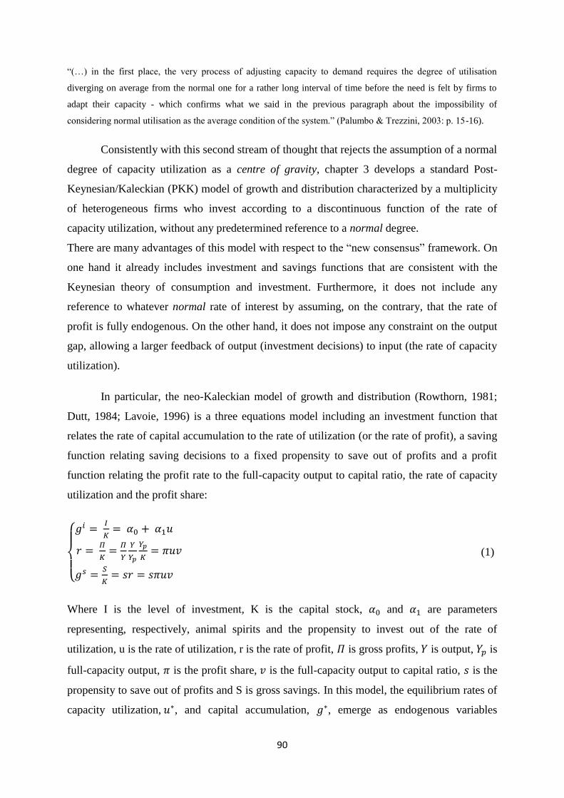
90

“(…) in the first place, the very process of adjusting capacity to demand requires the degree of utilisation

diverging on average from the normal one for a rather long interval of time before the need is felt by firms to

adapt their capacity - which confirms what we said in the previous paragraph about the impossibility of

considering normal utilisation as the average condition of the system.” (Palumbo & Trezzini, 2003: p. 15-16).

Consistently with this second stream of thought that rejects the assumption of a normal

degree of capacity utilization as a centre of gravity, chapter 3 develops a standard Post-

Keynesian/Kaleckian (PKK) model of growth and distribution characterized by a multiplicity

of heterogeneous firms who invest according to a discontinuous function of the rate of

capacity utilization, without any predetermined reference to a normal degree.

There are many advantages of this model with respect to the “new consensus” framework. On

one hand it already includes investment and savings functions that are consistent with the

Keynesian theory of consumption and investment. Furthermore, it does not include any

reference to whatever normal rate of interest by assuming, on the contrary, that the rate of

profit is fully endogenous. On the other hand, it does not impose any constraint on the output

gap, allowing a larger feedback of output (investment decisions) to input (the rate of capacity

utilization).

In particular, the neo-Kaleckian model of growth and distribution (Rowthorn, 1981;

Dutt, 1984; Lavoie, 1996) is a three equations model including an investment function that

relates the rate of capital accumulation to the rate of utilization (or the rate of profit), a saving

function relating saving decisions to a fixed propensity to save out of profits and a profit

function relating the profit rate to the full-capacity output to capital ratio, the rate of capacity

utilization and the profit share:

(1)

Where I is the level of investment, K is the capital stock, and are parameters

representing, respectively, animal spirits and the propensity to invest out of the rate of

utilization, u is the rate of utilization, r is the rate of profit, is gross profits, is output, is

full-capacity output, is the profit share, is the full-capacity output to capital ratio, is the

propensity to save out of profits and S is gross savings. In this model, the equilibrium rates of

capacity utilization, , and capital accumulation, , emerge as endogenous variables

91

dependent on the structural parameters of the investment function, and , and on the

structural parameters of the saving function, , and . For instance, by imposing the

equilibrium condition according to which investments equal savings, we get the following

equilibrium equations:

(2)

A graphical representation of the model helps to analyze its main properties:

Figure 3.1: representation of the paradoxes of thrift and costs in the neo-Kaleckian model of growth

An increase in the profit share (i.e. a fall in the real wage at constant labor

productivity), rather than increasing employment and output will raise the savings function

and lower the equilibrium rates of utilization and accumulation, consistently with the

“paradox of costs” (Rowthorn, 1981). An increase in the propensity to save out of profits,

rather than increasing investments and ouput will also raise the savings function and lower the

equilibrium rates of utilization and accumulation, consistently with the “paradox of thrift”

(ibid). The paradoxes of profits and thrift are based therefore on the assumption that the rate

of utilization is endogenous, and that a change in the structural parameters of the equation

implies a change in the final equilibrium.

The model in chapter 3 represents a micro-foundation of the savings and investment

functions of the neo-Kaleckian model of growth and distribution. Consistently with section 2,

it assumes that firms are subject to uncertainty and sunk costs (Dixit, 1989). Nevertheless,

when they decide to enter into a market they do not only engage in a one-for-all investment

92

decision, but in a series of investment decisions that imply a certain rate of growth of

productive capacity. In other words, firms do not target a specific level of capital stock, but

they rather target a range of desired rates of growth of productive capacity in a long time

horizon. According to Crotty (1993), for instance, because of sunk costs and worldwide

competition firms are coerced to invest, because if they do not invest they risk exiting from

the market. Furthermore, to the extent that sunk costs effects (Arkes & Blumer, 1985;

Garland, 1990) push firms to continue investing in a certain project in which they already

invested, the rate of utilization must be sufficiently low or sufficiently high to induce a change

in investment plans, by creating a range of rates of capacity utilization consistent with the

stability of a planned degree of growth (see section 4 for a larger development of the coerced

investments and sunk costs effects arguments). Consequently, firms’ investment decisions

depend discontinuously on the degree of capacity utilization, according to a disinvestment and

an investment thresholds that take into account heterogeneous sunk costs and heterogeneous

expectations. By introducing a discontinuous investment function of this type, transitory

shocks to the propensity to save out of profits, to the real wage and to animal spirits imply

permanent shocks to the rate of utilization, the rate of capital accumulation and the rate of

unemployment.

The novelty of this model with respect to the literature on genuine hysteresis is that it

does not assume a cumulatively neutral input that produces a hysteretic output, it rather

obtains a hysteretic input that produces a hysteretic output because of transitory shocks to the

propensity to save out of profits, to income distribution and to firms’ animal spirits.

Hysteresis in the rate of capacity utilization (the input) can be characterized as an emergent

property of the model, which implies the long run validity of the paradoxes of thrift and costs

despite the transitory nature of shocks. Consequently, the model provides a plausible

justification for rejecting the assumption of a unique and fixed normal degree of capacity

utilization, in favor of a range of rates of capacity utilization and capital accumulation around

which the economy might fluctuate persistently. Furthermore, it provides an explanation of

how transitory demand shocks can have permanent effects on the long run trajectory of the

economy, consistently with the empirical evidence of stably lower rates of growth, lower rates

of inflation and higher rates of unemployment in most European countries after the 2008’

financial crunch. The remainder of the chapter is organized as follows: section 3.2 is a

literature review about the structure and the fundamental properties of the Kaleckian model of

growth and distribution; section 3.3 presents a simple agent-based PKK model of growth and

93

distribution with genuine hysteresis; section 3.4 shows how the system reacts when submitted

to aggregate demand shocks; section 3.5 concludes.

3.2. A simple path-dependent agent-based PKK model of growth and

distribution

Applications of the standard genuine hysteresis model to economics are mainly about

international trade on the one hand (Amable et al, 1995) and unemployment on the other hand

(Piscitelli et al, 2000; Cross et al, 1998; De Peretti & Lang, 2009). Cross et al (2012) extended

the model of genuine hysteresis to potential output. In models dealing with unemployment,

the economic intuition relies on the existence of sunk costs in hiring decisions that make firms

adjust discontinuously to price. While in models dealing with international trade, the main

focus is about sunk costs in investment decisions and real exchange rate fluctuations (Dixit,

1989).

Consistently with the standard model of genuine hysteresis as applied in sciences like

physics and biology, however, most13

of these models assume an exogenous input in order to

focus on the emergent discontinuity of output to exogenous input shocks, and neglect the

difficult issue of the feedback mechanisms running from the output to the input. This

hypothesis, which can make sense under some circumstances for some systems in physics,

might prove problematic in economic systems. For example, if demand increases, investment

may also increase and it does not really make sense to suppose that this increase will not have

any influence on demand. Therefore, the feedback should be taken into consideration and this

is precisely what the model does.

In the wake of Cross et al (2012), this model of genuine hysteresis investigates the

economic conditions that are required to have persistent suboptimal equilibria in

unemployment and capital accumulation, despite the temporary nature of macroeconomic

shocks. Nevertheless, the input is fully endogenous and it is represented by aggregate

demand, proxied by the rate of utilization of productive capacity, while the output variable is

the rate of capital accumulation. Since investment decisions of firms imply production

decisions by other firms, capital accumulation affects effective demand and, as a

13

To our knowledge, Piscitelli et al (2000) is the first and only attempt to produce a model of genuine hysteresis

with endogenous input.

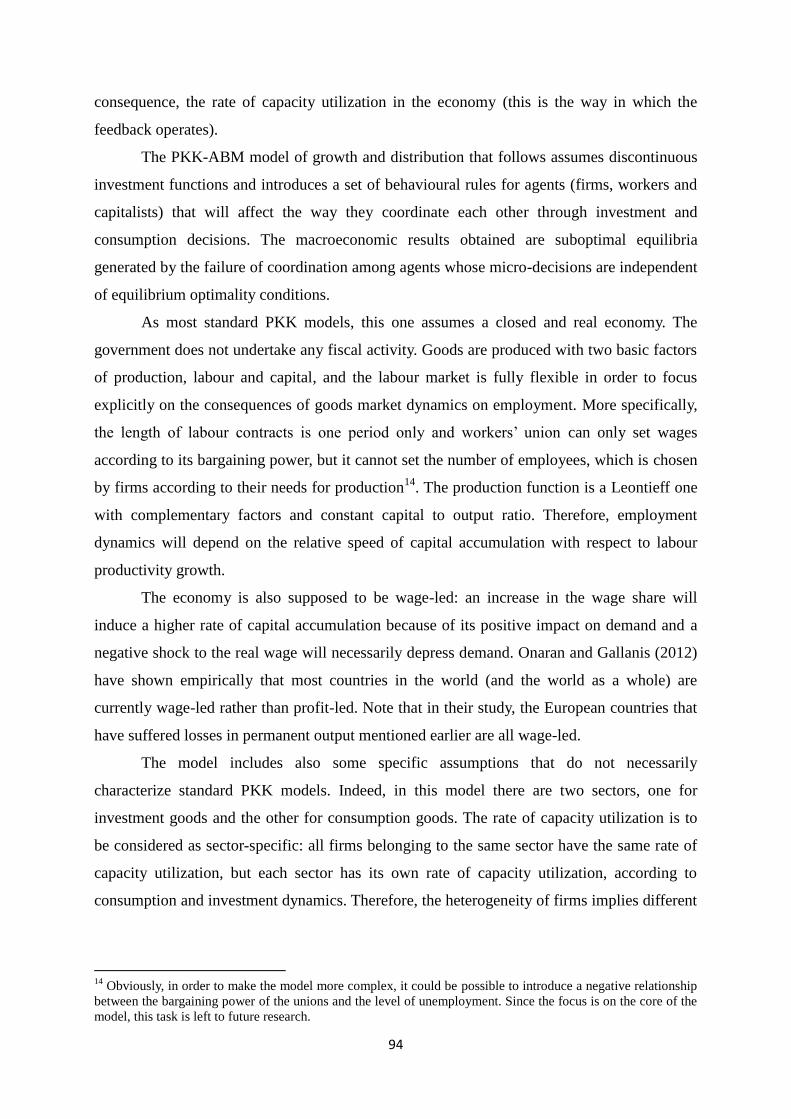
94

consequence, the rate of capacity utilization in the economy (this is the way in which the

feedback operates).

The PKK-ABM model of growth and distribution that follows assumes discontinuous

investment functions and introduces a set of behavioural rules for agents (firms, workers and

capitalists) that will affect the way they coordinate each other through investment and

consumption decisions. The macroeconomic results obtained are suboptimal equilibria

generated by the failure of coordination among agents whose micro-decisions are independent

of equilibrium optimality conditions.

As most standard PKK models, this one assumes a closed and real economy. The

government does not undertake any fiscal activity. Goods are produced with two basic factors

of production, labour and capital, and the labour market is fully flexible in order to focus

explicitly on the consequences of goods market dynamics on employment. More specifically,

the length of labour contracts is one period only and workers’ union can only set wages

according to its bargaining power, but it cannot set the number of employees, which is chosen

by firms according to their needs for production14

. The production function is a Leontieff one

with complementary factors and constant capital to output ratio. Therefore, employment

dynamics will depend on the relative speed of capital accumulation with respect to labour

productivity growth.

The economy is also supposed to be wage-led: an increase in the wage share will

induce a higher rate of capital accumulation because of its positive impact on demand and a

negative shock to the real wage will necessarily depress demand. Onaran and Gallanis (2012)

have shown empirically that most countries in the world (and the world as a whole) are

currently wage-led rather than profit-led. Note that in their study, the European countries that

have suffered losses in permanent output mentioned earlier are all wage-led.

The model includes also some specific assumptions that do not necessarily

characterize standard PKK models. Indeed, in this model there are two sectors, one for

investment goods and the other for consumption goods. The rate of capacity utilization is to

be considered as sector-specific: all firms belonging to the same sector have the same rate of

capacity utilization, but each sector has its own rate of capacity utilization, according to

consumption and investment dynamics. Therefore, the heterogeneity of firms implies different

14

Obviously, in order to make the model more complex, it could be possible to introduce a negative relationship

between the bargaining power of the unions and the level of unemployment. Since the focus is on the core of the

model, this task is left to future research.

95

investment rules and different rates of capital accumulation in a common aggregate demand

environment.

3.2.1. Sunk costs, strategic decisions and switching values

Investment decisions are generally taken in a genuinely uncertain environment

(Keynes, 1921), and they imply sunk costs that cannot be recovered if the investment decision

is reverted (Dixit, 1989). Generally speaking, firms invest in productive capital if expected

returns exceed expected costs. However, to the extent that some costs are fixed and cannot be

recouped if the investment fails (sunk costs), firms will require a minimum level of capacity

utilization sufficiently high to make the risk of having net losses fully compensated.

Furthermore, if a firm decides to invest but capacity utilization turns out to be lower than

expected ex post, before disinvesting it will make sure that the costs of dismissing the

excessive capital are lower than the costs of under-utilizing the whole capacity.

Formally firms’ investment criterion is (see section 1.3.3.):

(1)

With

. R stands for expected income, C for expected variable

costs, u for capacity utilization, r for the rate of time preference, SK for the sunk costs and

for the expected profits of not to invest. The letters with a star indicate expected income,

expected costs and expected rate of utilization if the investment is not undertaken.

The reason of this investment specification is quite intuitive: when the firm has to

decide whether to increase or not to increase productive capacity, the expected profits must be

higher than the sunk costs related to the new capital goods purchased and to the costs of

pushing capacity utilization upwards. The variable , for instance, is expected to capture all

the micro-, macro- and meso-economic reasons behind the decision of increasing or

decreasing capacity utilization, namely the desire to push capacity utilization up to the costs

minimizing rate, the possibility to rapidly satisfy peaks of demand by installing an excessive

productive capacity and the strategic decision to keep idle capacity as a deterrent to new

entrant firms (Kurz, 1986; Lavoie, 1996; Palumbo & Trezzini, 2003). Therefore, investment

decisions adjust discontinuously to aggregate demand shocks according to the sensitivity to

invest and according to the series of past shocks that affected firms’ investment decisions in

the past.

96

If a firm has already invested and has to decide whether to dismiss productive capacity

or not, the expected costs of keeping the same productive capacity need to be higher than the

costs of dismissing productive capacity, which are equal to unrecoverable costs and to micro-,

macro- and meso-economic costs of over-utilizing productive capacity. Formally, firms’

disinvestment criterion is the following:

(2)

Investment and disinvestment decisions of firms imply strategic considerations

concerning the expected rate of capacity utilization and the ex-post costs of reverting

investment decisions already undertaken; consequently, they are fundamentally not linear

with respect to external shocks that affect the rate of capacity utilization. In particular, by

defining the following equalities:

(3)

Both the investment and dismissing criteria can be formalized as direct functions of

the rate of capacity utilization:

(4)

Where and are the inverse functions of 15 irms will invest whenever

the rate of utilization is sufficiently high to make expected profits higher than expected costs,

and do not invest whenever the rate of utilization is sufficiently low to make expected profits

lower than expected costs.

3.2.2. Effective demand, expectations and the rate of capacity utilization

The rate of capacity utilization for firm i is equal to the ratio of production over productive

capacity:

(5)

15

For the sake of simplicity, is a reversible function as 0 < , where stands for the full rate of

capacity utilization. This assumption implies that expected profits are monotonic and increasing with respect to

the rate of capacity utilization when this latter lies below the full rate.

97

There are two sectors: firms can produce either consumption or capital goods.

Although firms belonging to the same sector are heterogeneous with respect to their switching

values (for investing or disinvesting) and with respect to their expectations, the model

assumes that they all face the same relative demand, proportionally with their size: big firms

will face a higher absolute demand with respect to small firms, but the rate of capacity

utilization will be the same. Consequently, the rate of capacity utilization is a sector-specific

variable: each firm faces the same rate of capacity utilization than all firms belonging to the

same sector16

.

As regards expectations, the model assumes that firms behave consistently with a

bounded, procedural rationality à la Simon (1972). Indeed, in a radical uncertain

environment, where individuals take decisions according to the limited set of information they

have, rational decisions are substituted with reasonable decisions, optimal choices with

satisficing choices, rational expectations with experience-based rules of thumb.

Consistently with most of Keynesian ABM models (Seppecher & Salle, 2015; Dosi et

al, 2013), firms estimate their future demand by looking at the variation of inventories: once

the ratio of inventories over productive capacity, , is equal to a desired reference ratio, ,

firms will only produce the quantity of goods that they expect to be sold, , which is equal

exactly to the variation of inventories, . Formally:

(6)

Expectations are sensitive to the discrepancy between the actual and the desired ratio

of inventories over productive capacity, consistently with a basic adaptive expectations

framework in which agents take decisions according to a simple rule-of-thumb based upon

past experience. In particular, if the actual ratio of inventories over productive capacity

increases over time, firms will interpret this excess of inventories as a lower-than-expected

demand, and will revise expectations downwards by producing at a lower rate of capacity

utilization. If, on the other hand, the actual ratio of inventories over productive capacity

decreases over time, firms will interpret this insufficiency of inventories as a higher-than-

expected demand and will revise expectations upwards by pushing the rate of capacity

utilization. Eventually, if the actual ratio of inventories over productive capacity is constant

16

The assumption of a unique rate of capacity utilization, however limiting, is made to focus on the way

heterogeneous firms react to a same aggregate shock. The aim of this model is not to reproduce business cycles

but rather to analyse how equilibria can permanently change in the wake of sectorial temporary shocks.

98

over time, firms will go on producing at the same rate of capacity utilization, since demand

was exactely equal to production.

Besides this backward-looking criterion, however, production decisions also depend

on a “irrational”, forward-looking component, which affects investment decisions and reflects

the Keynesian idea of “animal spirits”. In particular, investment decisions are modelled as a

function of an exogenous and constant component, which depends on firms’ “animal spirits”,

plus an additional component which depends on the expected rate of capacity utilization.

Therefore, when a firm is in equilibrium because the rate of stores over productive capacity is

constant and equal to the desired ratio, and , the rate of capacity utilization is the

same over time but the level of production is constantly increasing according to the pace of

capacity accumulation, which depends on the backward-looking component, the rate of

utilization, and a forward looking component, animal spirits. As a consequence, if firm i

decides to increase productive capacity and to produce in the future at the same rate of

capacity utilization, the future level of production will be equal to the past level of production

plus the expected increase in market demand, which is reflected in the decision to invest and

increase productive capacity.

3.2.3. Investment decisions and capital accumulation

By recalling (3) and (4) investment and disinvestment decisions can be represented as

fundamentally non-linear because of sunk costs and because of micro-, macro- and meso-

strategic choices. Diagram in figure 3.2, inspired by Amable et al (2004)17

, illustrates this

accumulation behaviour.

17

The model in Amable et al (2004) is a model of international trade with the exchange rate as input and the

export volume as output.

99

Figure 3.2: the rate of capital accumulation as a function of the rate of utilization

Investments in fixed capital at time t depend on the rate of capacity utilization, : if

expected net profits, which are a function of the rate of capacity utilization according to (3),

are higher than a, firms invest an amount of fixed capital which is proportional to the rate of

utilization.

However, even though the rate of utilization were to fall by making negative net

profits, firms would not decelerate capital accumulation unless net profits fell below b, by

making the costs of decelerating investment lower than the costs of underutilizing capacity.

Formally, the investment function for firm i is the following:

(7)

Where is the hysteresis operator that can take on value α or (α + β according to the

rate of capacity utilization:

(8)

Suppose for instance that a given firm produces at a rate of capacity utilization higher

than b but lower than a, and invests an amount of fixed capital equal to α . Suppose

now that demand suddenly increases and the increase is expected to last for a long period: to

the extent that the demand shock is sufficiently high to allow the firm pushing the rate of

capacity utilization upwards and increasing net expected profits above a, the rate of capital

β

α

α + (β

b a

100

accumulation will also shift upwards to (α + β in order to adjust productive capacity at a

higher level. If, however, a recession resulted in expected net profits falling back to the initial

level, the rate of capital accumulation would certainly fall to (α + β , with ,

but it would not revert to α unless the expected rate of capacity utilization fell below b.

Hence, the rate of accumulation would be permanently higher with respect to the

initial level, although the positive demand shock was only temporary and expectations were

eventually correctly revised, since the investment decision made in the aftermath of the

positive demand shock implied long-term sunk costs that cannot be recovered and that would

be lost is the firm decided to revise downwards investment decisions. Furthermore The same

applies if the firm produces at a rate of capacity utilization higher than b but lower than a, and

invests an amount of fixed capital equal to α . If demand suddenly falls below b,

the firms will decrease the rhythm of accumulation, and even though the rate of utilization

were to go back to , the firm would still be investing at a lower and constant rate,

that is . In this case, the rate of accumulation would be permanently lower with

respect to the initial level, since once capital has been dismissed, reaching the initial rythm of

accumulation would require a higher expected demand.

At the macroeconomic level, as the economy is made of several firms with different

sunk costs and different expectations, a given sequence of aggregate demand shocks will

imply different and discontinuous reactions in terms of capital accumulation, which might

cause hysteresis to occur.

3.2.4. Income distribution, employment and consumption decisions

Firms employ workers according to a standard Leontieff production function with

complementary factors and scarce capital. Therefore, a given amount of output is associated

with a given stock of capital and a given number of workers:

(9)

B represents the inverse of the capital to output ratio (the “productivity of capital”),

which is assumed to be constant and, for the sake of simplicity, equal to 1, while A represents

the inverse of the labour to output ratio (“labour productivity”). Therefore, employment

101

increases whenever the rate of capital accumulation exceeds the rate of growth of labour

productivity, and it decreases whenever labour productivity grows faster than capital

accumulation18

:

(10)

Labour productivity is a firm-specific variable: firms invest in labour saving and

innovative technologies in order to develop inter- and intra-organizational capabilities and

enhance the organization of labour resulting in a higher firm-specific productivity. The labour

productivity function is the following one:

(11)

Productivity at time t, is equal to productivity at time t-1, , plus the rate of

growth of labour productivity at time t, The rate of growth of labour productivity at time

t, on the other hand, is equal to the rate of growth of labour productivity at time t-1

plus the difference between the desired rate of growth of labour productivity

which is equal to the rate of capital accumulation , and the actual rate of growth of labour

productivity . According to the second and third equation in (11), firms aim to adapt the

rate of growth of labour productivity to the rate of growth of capital, which is the rate of

growth necessary to keep employment constant. The parameter reflects the ability of firm i

to innovate and adapt labour productivity to capital accumulation: the more gets close to 1,

the easier firms can adapt labour productivity to capital accumulation19

.

Once firms employ workers, they pay wages20

according to the union’s targeted wage

rate, which is defined as a targeted share of the potential output to labour ratio

, and to

the bargaining power of the union, :

18

For the sake of simplicity, the rate of population growth is equal to 0 19

Although labor productivity is endogenous with respect to output, ε should not be interpreted as a

Verdoorn’s coefficient but rather as a firm specific capability to develop labor saving techniques. The rationale

of the function is that firms aim to push the rate of growth of labor productivity up to (or above) the rate of

capital accumulation in order to save on labor costs and accumulate more profits. From this point of view, the

rationale behind the idea of a “desired rate of labor productivity” is not different from the rationale behind the

idea of a “desired rate of capacity utilization”: they both represent intermediate requirements to achieve a

“desired rate of profit”. Appendix 3.2 provides a sensitivity analysis on the value of epsilon. 20

Since prices are constant and equal to 1, wages are expressed in real terms.

102

(12)

The bargaining power of unions, , is itself an increasing function of the rate of

employment (there is a “Phillips effect”), defined as the ratio of the employed persons to the

active population, plus an exogenous component which reflects institutional factors as well

as the monopolistic structure of the market:.

(13)

For the sake of simplicity, and in the baseline scenario, therefore the

bargaining power of unions is simply equal to the rate of employment21. This will imply that

when the employment rate approaches 100 %, the actual wage rate and the desired wage rate

coincide. When, on the other hand, the employment rate is weaker, the actual wage rate will

be consistently lower with respect to the targeted rate. Consequently, income distribution

ultimately depends on the employment rate (the balance of power between capitalists and

workers), that itself depends on the relative speed of capital accumulation with respect to

labour productivity growth.

The residual, that is the difference between value added and wages, is distributed to

capitalists, who take consumption and saving decisions according to their propensity to

consume, cK.

This model, according to the PKK literature and Kalecki’s own works, assumes a

propensity to consume out of wages equal to 1 and a propensity to consume out of profits

21

Equations (12) and (13) state that although the union might target a given wage share, , she will only get a

fraction of this target according to her bargaining power, which depends on the rate of employment and on the

broader institutional and economic environment. The bargaining power of the union therefore is implicitly

defined as the capacity of the union to bargain a wage bill that is consistent with the desired wage share. This

assumption does not necessarily require rational expectations, since the union does not bargain an equilibrium

real wage – she bargains a nominal wage bill, according to her expectations about future prices and to her

desired wage share, and will obtain ex post only a fraction of the desired wage share, which is not necessarily

the equilibrium wage share.

Note that PKK models often assume that the wage rate is a share of actual, rather than potential, “labour

productivity” (Hein, 2005). In these models, for instance, the rate of employment is a function of the rate of

capacity utilization, while in this model employment at the firm level is determined by the rate of capital

accumulation, not by the rate of capacity utilization. Nevertheless, it turns out that this micro model is perfectly

consistent with the results of standard macro PKK models. For instance, since the firm-specific rate of capacity

utilization determines the firm-specific rate of capital accumulation, at the macro level the aggregate wage rate is

still a function of the aggregate rate of capacity utilization and, therefore, of actual labour productivity.

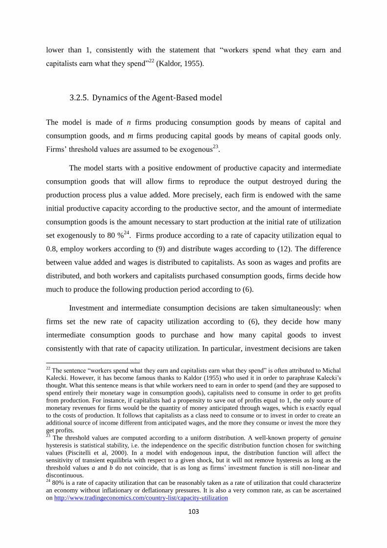
103

lower than 1, consistently with the statement that “workers spend what they earn and

capitalists earn what they spend”22

(Kaldor, 1955).

3.2.5. Dynamics of the Agent-Based model

The model is made of n firms producing consumption goods by means of capital and

consumption goods, and m firms producing capital goods by means of capital goods only.

Firms’ threshold values are assumed to be exogenous23

.

The model starts with a positive endowment of productive capacity and intermediate

consumption goods that will allow firms to reproduce the output destroyed during the

production process plus a value added. More precisely, each firm is endowed with the same

initial productive capacity according to the productive sector, and the amount of intermediate

consumption goods is the amount necessary to start production at the initial rate of utilization

set exogenously to 80 %24

. Firms produce according to a rate of capacity utilization equal to

0.8, employ workers according to (9) and distribute wages according to (12). The difference

between value added and wages is distributed to capitalists. As soon as wages and profits are

distributed, and both workers and capitalists purchased consumption goods, firms decide how

much to produce the following production period according to (6).

Investment and intermediate consumption decisions are taken simultaneously: when

firms set the new rate of capacity utilization according to (6), they decide how many

intermediate consumption goods to purchase and how many capital goods to invest

consistently with that rate of capacity utilization. In particular, investment decisions are taken

22

The sentence “workers spend what they earn and capitalists earn what they spend” is often attributed to Michal

Kalecki. However, it has become famous thanks to Kaldor (1955) who used it in order to paraphrase Kalecki’s

thought. What this sentence means is that while workers need to earn in order to spend (and they are supposed to

spend entirely their monetary wage in consumption goods), capitalists need to consume in order to get profits

from production. For instance, if capitalists had a propensity to save out of profits equal to 1, the only source of

monetary revenues for firms would be the quantity of money anticipated through wages, which is exactly equal

to the costs of production. It follows that capitalists as a class need to consume or to invest in order to create an

additional source of income different from anticipated wages, and the more they consume or invest the more they

get profits. 23

The threshold values are computed according to a uniform distribution. A well-known property of genuine

hysteresis is statistical stability, i.e. the independence on the specific distribution function chosen for switching

values (Piscitelli et al, 2000). In a model with endogenous input, the distribution function will affect the

sensitivity of transient equilibria with respect to a given shock, but it will not remove hysteresis as long as the

threshold values a and b do not coincide, that is as long as firms’ investment function is still non-linear and

discontinuous. 24

80% is a rate of capacity utilization that can be reasonably taken as a rate of utilization that could characterize

an economy without inflationary or deflationary pressures. It is also a very common rate, as can be ascertained

on http://www.tradingeconomics.com/country-list/capacity-utilization

104

according to (8), while intermediate consumption decisions are taken according to a linear

function of expected production:

(14)

Where I.C. stands for “intermediate consumption” and is a constant parameter representing

the fraction of output needed for intermediate consumption25

.

As soon as investment and intermediate consumption decisions are taken, firms

purchase capital and intermediate consumption goods and observe the variation of inventories

in order to estimate their global demand.

The following production period will start by producing at the rate of capacity

utilization set in (6), employing workers according to (9), paying wages according to (12) and

restarting the whole process as described above.

3.3. Emergent properties and reaction to shocks

The baseline scenario reflects the main reference properties of the model as regards

employment dynamics, income distribution, capacity utilization and capital accumulation. By

simulating simulate macro- or micro- economic shocks it is possible therefore to observe how

the economy reacts with respect to the baseline scenario behaviour, in particular as regards the

inability of the system to absorb the shocks and regain the initial growth path26

.

In order to try to keep the model as close to reality as possible, the values of some

parameters have been chosen according to empirical estimates and to macroeconomic

empirical trends. Namely, the baseline’s scenario tries to reproduce the rates of capacity

utilization, capital accumulation and unemployment, as well as income distribution of the

French economy during expansionary periods. 27

25

The specific value of assumed during the simulations of the model in section 3 is inspired by Storm and

Naastepad (2015). 26

All simulations have been implemented under Netlogo 5.1.0. The program is available from the authors upon

request. 27

Appendix 3.1 summarizes the values of the parameters.

105

As simple and modest as the model might be, it may help to shed light on the current

situation in many European countries and in particular the one that have suffered losses in

potential output mentioned in section 1.2.1.

3.3.1. The “paradox of costs” and the consequence of cuts in the real wage

According to the mainstream view (see for example Layard et al, 1991), the rate of

unemployment is positively related to the wage rate; therefore, lowering the unit labour costs

of firms is supposed to foster new hiring and boosting employment because of a supply-side

stimulus to the economy. From an economic policy standpoint, this is the “internal

devaluation” strategy that has been followed since 2009 in many southern European countries

like Greece, Portugal, Spain or Italy.

The “paradox of costs” highlights on the contrary that, as wages are a significant part

of income for most households, lowering real wages implies lowering aggregate demand and

hence the incentives to invest (Rowthorn, 1981; Storm & Naastepad, 2012; Lavoie, 2014). As

a consequence we should expect the opposite result to dominate: lower real wages should be

associated with a lower rate of capacity utilization and a lower rate of capital accumulation.

The simulations implemented show that the “paradox of costs” holds – and therefore,

why the internal devaluation strategies are a failure.

Figure 3.3: capital accumulation in the wake of a negative shock to unions’ bargaining power

106

Figure 3.4: the rate of utilization in the wake of a negative shock to unions’ bargaining power

Figure 3.5 the employment rate in the wake of a negative shock to unions’ bargaining power

Figures 3.3 to 3.5 show the effect of a fall in the real wage to the rate of capacity

utilization, to capital accumulation and to the employment rate.

At time t=15, a temporary negative shock to the exogenous component of the

bargaining power of unions ( = -0.1) in both sectors triggers a fall in aggregate capacity

utilization and, consequently, in the rate of capital accumulation. At time t=65 the shock is

over but the economy does not regain the baseline’s growth path: the rates of capacity

utilization and capital accumulation, as well as the rate of employment, are permanently lower

with respect to the baseline scenario, although the shock was only temporary.

The effect on productive capacity is therefore a permanent loss in the level and in the

rate of growth, as shown in figure 3.6.

107

Figure 3.6: potential output in the wake of a negative shock to unions’ bargaining power

As illustrated in figure 3.6, potential output falls below its baseline growth path and

stabilizes at a lower level and a lower rate of growth – which is consistent with Ball’s findings

regarding Spain, Italy, Greece and Portugal.

The hysteresis effect on potential output growth can be explained through the effect of

a temporary negative demand shock on firms’ investment decisions. Since the propensity to

consume out of wages is higher than the propensity to consume out of profits, a fall in the real

wage implies a net fall in aggregate consumption and, thereby, in the rate of capacity

utilization. Some firms will react to the negative demand shock by reducing the rhythm of

accumulation and firing workers until productivity growth slows down and keeps up with the

lower accumulation pace. As a consequence of the lower rate of employment, the real wage

will fall even further until the negative shock is over and aggregate demand starts to increase

again because of the increase in the real wage. However, some firms will not revert to the

previous accumulation path despite the increase in aggregate demand as long as the rate of

capacity utilization is too low to trespass the investment threshold a. These firms will only

increase the rate of capacity utilization without increasing investments and employment. A

negative temporary shock to the real wage therefore implies a shift to a new equilibrium

characterised by a lower level of potential output and lower rates of capacity utilization,

capital accumulation and employment.

3.3.2. The “paradox of thrift” and the Fisher effect

According to mainstream theory of growth, the rate of capital accumulation is

positively related to the propensity to save either in the short- (Solow, 1956) or in the long run

(Frankel, 1962; Romer, 1990).

108

In the PKK literature on growth and distribution (Rowthorn, 1981; Dutt, 1984; Lavoie,

1996, 2014) however, savings do not directly determine investments to the extent that the

latter are independent on the propensity to save and only depend on the rate of capacity

utilization, the “Keynesian Hypothesis” (Kaldor, 1955). In such a situation, increasing savings

would not foster accumulation but would rather have the opposite result: as long as the

aggregate propensity to consume falls, capital accumulation slows down because of the lower

aggregate demand and the lower rate of capacity utilization. This negative effect of savings on

capital accumulation has been defined as the paradox of thrift. The model, consistently with

the PKK tradition, exhibits the paradox of thrift (see figures 3.7 to 3.9):

Figure 3.7: capital accumulation after a negative shock to capitalists’ propensity to consume

Figure 3.8: The rate of capacity utilization after a negative shock to capitalists’ propensity to consume

Figure 3.9: The employment rate after a negative shock to capitalists’ propensity to consume

109

Figures 3.7 to 3.9 show the effects on capacity utilization and capital accumulation of

a negative shock to the propensity to consume out of profits. At time t=15, capitalists become

more virtuous in the sense of Smith (1776): they increase the propensity to save out of profits

by 12%. As a consequence of the lower aggregate consumption the rates of capacity

utilization, capital accumulation and employment start to fall until capitalists keep on saving

at the initial rate and the economy stabilizes at a new equilibrium characterized by a lower

rate of utilization, a lower rate of capital accumulation and a lower rate of employment with

respect to the initial growth path. The effects on potential output can be observed in figure

3.10.

Figure 3.10 potential output after a negative shock to capitalists’ propensity to consume

In Figure 3.10, potential output falls below its initial growth path and stabilizes at a

lower level and a weaker rate of growth. Therefore, because of the discontinuity of investment

decisions that do not respond linearly to aggregate demand shocks, a negative temporary

shock to the propensity to consume out of profits implies a shift to a new equilibrium

characterised by a lower potential output and lower rates of capacity utilization, capital

accumulation and employment. Once again, the final equilibrium is history-dependent.

These results might be interpreted as an illustration of the Fisher (1933) effect: in

recessions like the current one, firms and households are deleveraging. As a consequence, the

saving propensity in the economy goes up, which depresses aggregate demand instead of

stimulating it.28

28

One has nevertheless to be cautious with this interpretation, as this economy is a real economy without any

financial and banking sector.

110

3.3.3. Animal spirits and the propensity to invest

A third characteristic of PKK models is the positive relationship between the

propensity to invest of firms and both the rates of capacity utilization and capital

accumulation. Consistently with the Keynesian view regarding animal spirits, if entrepreneurs

are caught by a wave of pessimism and decide to reduce autonomous investments, the rate of

capacity utilization falls because of the lower effective demand, and capital accumulation

consequently decelerates. The rates of capacity utilization and capital accumulation are

particularly sensitive to animal spirits.

Figure 3.11: the rate of capital accumulation after of a fall in entrepreneurs’ animal spirits

Figure 3.12: the rate of utilization after a fall in entrepreneurs’ animal spirits.

Figure 3.13: the employment rate after a fall in entrepreneurs’ animal spirits

111

Figures 3.11 to 3.13 show the effects on the rate of capacity utilization, the rate of

capital accumulation and the employment rate in the wake of a fall in animal spirits. At time

t=15 a negative temporary shock to animal spirits by 0.04 implies a fall in the rates of

capacity utilization, capital accumulation and employment. When at time t=65 entrepreneurs

keep on investing at the same secular pace, both the rates of capacity utilization and capital

accumulation start to increase again but not sufficiently to regain the baseline growth path: the

economy stabilizes at a new equilibrium characterised by a lower utilization, lower

employment and lower accumulation of productive capacity with respect to the initial

equilibrium. The effects on potential output can be observed in figure 3.14.

Figure 3.14: potential output in the wake of a fall in entrepreneurs’ animal spirits

As is clear from figure 3.14, even if the negative shock was only temporary, the effects

of the shock are long lasting, since the economy now stabilizes at a new equilibrium

characterised by a lower potential output level and a weaker rate of accumulation with respect

to the baselines’s growth path. Furthermore, both the rate of utilization and the rate of

employment are permanently lower.

This can once again shed light on the current situation of many European countries,

where, as a consequence of the recession, animal spirits are depressed, which has had

permanent consequences on potential output (see section 1.2.1).

3.4. Concluding remarks

In order to understand why potential output might suffer permanent losses in the

aftermath of negative shocks, this PKK-ABM model of capital accumulation and growth

assumed independent micro-decisions of heterogeneous firms generate history-dependent

112

aggregate outcomes. As it is clear from the simulations implemented, the model is consistent

with the “paradox of costs” and the “paradox of thrift”, and changes in animal spirits affect

the long-run path of the economy permanently. As a consequence, this simple model can shed

light on the loss of potential output in many European countries (Ball, 2014), which is the

consequence of a combination of internal devaluation policies, the Fisher effect and depressed

animal spirits.

This model contains several major innovations. Firstly, it relates three fields of

knowledge that usually ignore the one another: PKK models of growth and income

distribution, agent-based models and models of genuine hysteresis. Secondly, many papers on

genuine hysteresis or on agent-based modelling have discussed the feedback effect of the

output to the input without modelling it, while in this model the feedback effect is fully

integrated – a novel feature that seems to be most desirable in economics in general and in

this model in particular (as investment also influences aggregate demand). Thirdly, this

simple theoretical framework allows showing that, under the simple (and realistic) assumption

that heterogeneous firms adjust their rate of capital accumulation discontinuously, temporary

shocks to the economy will have permanent effects on potential output: history matters and

time is clearly historical time. As a consequence, there is no reason to expect potential output

going back to its pre-crisis level in the aftermath of shocks.

The behaviour of potential output appears to be in line with the pattern observed by Ball

(2014) in many European countries, that is, a permanent fall in potential output. The

economic policy implication is most clear: if we want potential output to reach its pre-crisis

level again, an exogenous economic policy intervention is needed. In this model, it means that

authorities have to implement a shock in order to make sure that multiple firms will cross the

α threshold by changing the animal spirits in a positive way (for example by announcing an

expansionary fiscal policy), by increasing the capitalists’ propensity to consume (possibly by

solving the deleveraging issue by writing off some debt) or by affecting income distribution in

favour of wage-earners (by raising real wages, for example on the basis of a rise in the

minimum wage; or by reinforcing unions and workers’ rights).

Nevertheless, the model has several limitations. All of them might constitute leads for

future research. Firstly, like in the seminal paper by Dutt (1984), the economy is wage-led. As

mentioned earlier, this can be justified by the empirical findings of Onaran and Galanis

(2012). But Bhaduri and Marglin (1990) have shown that economies can also be profit-led

when the depressive effect of a falling wage share on consumption can be more than

113

compensated by the expansionary effect of the increasing profit share on investment. And as

wage-led economies can become profit-led under some circumstances, and to cover the full

range of possible situations, it would nevertheless be interesting to have both cases included

in future models.

Secondly, the dynamics of prices are not taken into account. From that perspective, the

bargaining/conflict part of the model needs to be enriched, for example along the lines

suggested by Cassetti (2003) or Lavoie (2014). This is crucial if one wants to analyse how

functional and personal income distribution are shaped in the economy and the permanent

effects conflicts can have on the rates of growth, on capital utilization and on inflation. In

order to reinforce this part of the model, one could also allow, in a more realistic fashion, to

let the bargaining power of workers change with the rate of unemployment.

Thirdly, as population growth is left out of the model, the Verdoorn coefficient was

supposed to be equal to unity at the equilibrium. Allowing the population to grow would

allow introducing the consequences of capital accumulation on productivity consistently with

Kaldor’s and Verdoorn’s empirical findings.

Fourthly, the way in which expectations and bounded rationality are can be

complexified. For example, using “boundedly rational” expectations based on an artificial

neural networks (Salle, 2015) is likely to generate richer and more complex dynamics and

might prove interesting for future research.

Last but not least, like most PKK models, this one is a purely real one, in which both

capitalists and workers are paid in real terms. In the absence of money, credit and banks, this

economy is not a monetary economy of production. Even if firms are never constrained by the

available amount of savings, they are not allowed to borrow in order to invest and produce

either, while in actual economies money, credit and banking play a central role. The very

presence of money and banking may allow for a dynamics of credit and private debt which

can lead to endogenous cycles (Keen, 1995). It could then be possible to fully examine the

consequence of the debt-deflation mechanisms à la Fisher in the presence of genuine

hysteresis. This is an avenue for future research. Including credit in the model would be an

important progress: even if the input is endogenous, the various shocks under consideration

are still exogenous while in reality multiple shocks are endogenous by nature.

Next chapter will specifically focus on some of these evolutions, namely including a banking

sector and a credit channel; including both real and nominal growth; introducing bargaining

114

conflict in the model via a specific mark-up function; Moreover, the model in next chapter

will remove the assumption of a unique input allowing each firm to have a specific rate

market demand and a specific rate of capacity utilization.

115

Appendix 3.1: values of parameters

Description Parameter Value

Number of firms in consumption-goods sector n 500

Number of firms in capital-goods sector m 500

Active population AP 9150

Initial capital stock of firms in consumption-goods

sector

10

Initial capital stock of firms in capital-goods sector 1

Union’s desired wage rate in consumption-goods

sector

0.2

Union’s desired wage rate in capital-goods sector 0.6

Accelerating investment threshold a = f’( ) Random ~ U(0.5, 0,9)

Decelerating investment threshold b = f’( ) Random ~ U(0.5, )

Desired ratio of inventories over productive capacity 0.8

Exogenous investment parameter α 0.005

Propensity to invest as a share of production β 0.05

Share of intermediate consumption goods 0.67

Firms’ ability to increase the output to labour ratio ε 0.1

Potential output to capital ratio B 1

Initial output to labour ratio 1

Sensitivity of unions’ bargaining power to the

employment rate

1

Propensity to consume out of wages 1

Propensity to consume out of profits 0.25

116

Appendix 3.2: sensitivity analysis

Figure 3.15: employment rate in the wake of a temporary negative shock to animal spirits by 0.05. Sensitivity

analysis with respect to ε

Figure 3.16: employment rate in the wake of a temporary negative shock to the bargaining power of unions by

0.08. Sensitivity analysis with respect to ε

Figure 3.17: employment rate in the wake of a temporary negative shock to the propensity to consume out of

profits by 0.15. Sensitivity analysis with respect to ε

0.08 0.1 0.12

0.08 0.1 0.12

0.08 0.1 0.12

0.15 0.2 Baseline

117

Figure 3.18: employment rate in the wake of a temporary negative shock to animal spirits. Sensitivity analysis

with respect to different intensities of shock

Figure 3.19: employment rate in the wake of a temporary negative shock to the bargaining power of unions.

Sensitivity analysis with respect to different intensities of shock

Figure 3.20: employment rate in the wake of a temporary negative shock to the propensity to consume out of

profits. Sensitivity analysis with respect to different intensities of shock

0.001 0.002 0.003 0.004 0.005 Baseline

0.02 0.04 0.06 0.08 0.1 Baseline

0.03 0.06 0.09

118

Figure 3.21: rate of capacity utilization in the wake of a temporary negative shock to animal spirits. Sensitivity

analysis with respect to different intensities of shock

Figure 3.22 rate of capacity utilization in the wake of a temporary negative shock to the bargaining power of

unions. Sensitivity analysis with respect to different intensities of shock

Figure 3.23: rate of capacity utilization in the wake of a temporary negative shock to the propensity to consume

out of profits. Sensitivity analysis with respect to different intensities of shock

0.001 0.002 0.003 0.004 0.005 Baseline

0.02 0.04 0.06 0.08 0.1 Baseline

0.03 0.06 0.09 0.12 0.15 Baseline

119

Figure 3.24: rate of capital accumulation in the wake of a temporary negative shock to animal spirits. Sensitivity

analysis with respect to different intensities of shock

Figure 3.25: rate of capital accumulation in the wake of a temporary negative shock to the bargaining power of

unions. Sensitivity analysis with respect to different intensities of shock

Figure 3.26: rate of capital accumulation in the wake of a temporary negative shock to the propensity to

consume out of profits. Sensitivity analysis with respect to different intensities of shock

0.001 0.002 0.003 0.004 0.005 Baseline

0.02 0.04 0.06 0.08 0.1 Baseline

0.03 0.06 0.09 0.12 0.15 Baseline

120

4. Coerced investments, growth/safety trade-off and the stabilizing role of demand policies. An Agent-based stock flow consistent model of endogenous business cycles and structural change

4.1. Introduction

Chapter 3 developed a simple Post-Keynesian/Kaleckian agent-based model with

genuine hysteresis to show that transitory shocks to the propensity to save out of profits, to the

real wage or to firms’ animal spirits may not cancel out and imply a permanent change in the

degree of capacity utilization, in the rate of unemployment and in the rate of capital

accumulation. This happens when some firms standing in their zone of inaction permanently

change their accumulation strategy in the wake of transitory shocks (see chapter 2). As a

consequence, the model in chapter 3 supports the possibility to observe the economy

fluctuating within a range of possible rates of capacity utilization, without triggering any

endogenous mechanism of adjustment towards a predetermined normal degree. As a

consequence, the paradoxes of costs and thrift hold in a long run horizon even when shocks

are only transitory. Chapter 3 concludes by arguing that a recession followed by austerity

measures will lead to a permanent loss of productive capacity. Furthermore, according to the

property of remanence, exiting from the crises requires that positive demand shocks be more

than proportionally higher with respect to the negative demand shocks that brought about the

recession.

The model of chapter 3, however, did not include a fiscal or a monetary policy

framework, consequently the conclusion was not supported by specific simulations.

Moreover, it made other simplifying assumptions that chapter 4 relaxes in order to increase

the level of complexity of the whole framework and extend the validity of the model. Namely,

the model assumed for simplicity fixed prices and wages. Furthermore, it assumed a common

sector-specific degree of capacity utilization for all firms, in order to focus on the

discontinuity of capacity adjustments with respect to a common input, consistently with

121

standard models of genuine hysteresis. As a consequence, the artificial economy of chapter 3

evolves on steady rates of capacity utilization, capital accumulation and unemployment,

unless an exogenous transitory shock implies a disequilibrium process and then the

convergence towards a new steady state. Thanks to this simplifying framework, however, it is

possible to focus specifically on the properties of genuine hysteresis when feedback

mechanisms running from output to input are explicitly taken into account. In particular, the

model shows that hysteresis is contingent to two main assumptions: namely that labour

productivity adjusts relatively slowly to capital accumulation and that the real wage is a

function of unemployment. For instance, if labour productivity adjusted immediately to

capital stock variations, a transitory shock would have no impact on the rate of unemployment

and thereby on real wages. Consequently, we would observe the economy adjusting back to

the initial steady state, without exhibiting hysteresis (see chapter 3 and Appendix 3.2). The

same applies if real wages were independent from unemployment: in such a case, a transitory

demand shock would have no permanent effect on the rates of utilization and capital

accumulation, even though the rate of unemployment were permanently lower or higher. In

other words, the chain of causalities that generate hysteresis starts from the discontinuity of

investment decisions, which generates permanent variations of the rate of unemployment and,

thereby, permanent variations in real wages. Consequently, the rate of capacity utilization and

the rate of capital accumulation stabilize at a different steady rate. In chapter 4, these two

assumptions - the relatively slow adjustment of productivity to capital accumulation and the

pro-cyclical nature of real wages – will be retained. Nevertheless, the whole framework will

be more complex. Namely, the model introduces a government and a monetary sector in order

to take into account the effects of monetary and fiscal policies explicitly; it also assumes that

wages and prices evolve endogenously, and that the rate of capacity utilization can be

different for each firm, according to its price and its size. The model of chapter 4 will be

mostly based on Dosi et al (2015), Assenza et al (2014) and Seppecher & Salle (2015). In

these models, however, investment decisions are linear and depend on the discrepancy

between actual and normal degree of capacity utilization, while the model of chapter 4 will

assume a non linear and discontinuous investment function according to the genuine

hysteresis framework developed in chapter 3.

In the recent macroeconomic mainstream literature based on the Real Business Cycles

(RBC) or Dynamic Stochastic General Equilibrium (DSGE) approaches, which generally

assume linear and continuous investment decisions, output fluctuations are explained through

122

non-stationary and ad hoc technological shocks to potential output in a perfect competition

framework characterized by full flexibility of prices and wages (Kydland & Prescott, 1982;

King, Plosser & Rebelo, 1988; King & Rebelo, 2000) or in a imperfect competition

framework characterized by friction in wages and price adjustments (Smets & Wouters, 2003;

Justiniano & Primiceri, 2009; Vetlov et al, 2011). Despite the theoretical and methodological

differences in these two approaches, we find some common patterns, namely that the output

gap is equal to zero in the long run, despite transitory deviations, and consequently that

permanently lower equilibrium rates of growth or output levels can only be explained through

exogenous supply shocks, either stationary of non-stationary, affecting the level of capital

rather than its degree of utilization. Consistently with this general framework, a growing

stream of research has introduced some forms of non-linearity and discontinuity in capital

stock adjustments at the micro-level in order to account for the empirically observed

variability of aggregate investments during business cycles (Caballero & Pindyck, 1992;

Bertola & Caballero, 1994; Abel & Eberly, 1999; Caballero & Engel, 1999; Veracierto, 2002;

Thomas, 2002; Kahn & Thomas, 2008; Bachman et al, 2013). In particular, we can

distinguish different approaches to discontinuity in investment decisions based on the (S,s)

model. Caballero & Pindyck (1992), Bertola & Caballero (1994) and Abel & Eberly (1999)

analyze the behaviour of firms with irreversible investments. In these models, firms can only

increase their capital stock if it is lower than a certain optimal, or desired level, but they

cannot scrap capital if they are caught with excess capacity except just letting capital

depreciating at a fixed and constant rate (Abel & Eberly, 1999) rule out capital depreciation).

In particular, Abel & Eberly (1999) assumes the existence of a trigger value for the

marginal efficiency of capital above which firms increase their capital stock in order to bring

back the marginal efficiency to the user cost of capital, and below which firms are inactive.

This trigger value, consistently with Dixit (1989), depends on uncertainty and on the unit cost

of capital.

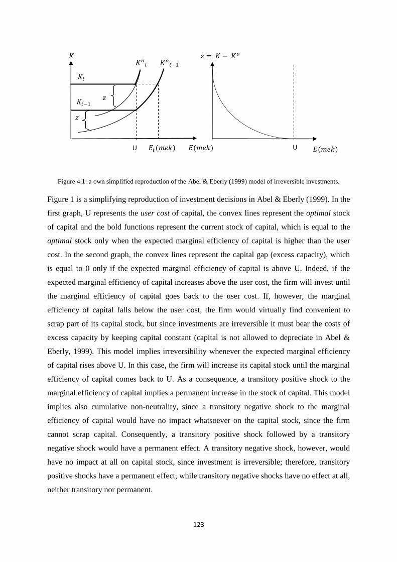
123

Figure 4.1: a own simplified reproduction of the Abel & Eberly (1999) model of irreversible investments.

Figure 1 is a simplifying reproduction of investment decisions in Abel & Eberly (1999). In the

first graph, U represents the user cost of capital, the convex lines represent the optimal stock

of capital and the bold functions represent the current stock of capital, which is equal to the

optimal stock only when the expected marginal efficiency of capital is higher than the user

cost. In the second graph, the convex lines represent the capital gap (excess capacity), which

is equal to 0 only if the expected marginal efficiency of capital is above U. Indeed, if the

expected marginal efficiency of capital increases above the user cost, the firm will invest until

the marginal efficiency of capital goes back to the user cost. If, however, the marginal

efficiency of capital falls below the user cost, the firm would virtually find convenient to

scrap part of its capital stock, but since investments are irreversible it must bear the costs of

excess capacity by keeping capital constant (capital is not allowed to depreciate in Abel &

Eberly, 1999). This model implies irreversibility whenever the expected marginal efficiency

of capital rises above U. In this case, the firm will increase its capital stock until the marginal

efficiency of capital comes back to U. As a consequence, a transitory positive shock to the

marginal efficiency of capital implies a permanent increase in the stock of capital. This model

implies also cumulative non-neutrality, since a transitory negative shock to the marginal

efficiency of capital would have no impact whatsoever on the capital stock, since the firm

cannot scrap capital. Consequently, a transitory positive shock followed by a transitory

negative shock would have a permanent effect. A transitory negative shock, however, would

have no impact at all on capital stock, since investment is irreversible; therefore, transitory

positive shocks have a permanent effect, while transitory negative shocks have no effect at all,

neither transitory nor permanent.

U U

124

Note that, in this model, investments do not exhibit lumpiness, since investment

decisions do not imply non-convex adjustment costs. That is, firms can increase their

productive capacity gradually without fixed costs. In order to take into account lumpiness and

costly reversibility, the (S,s) literature has introduced the existence of non-convex (i.e. fixed)

adjustment costs that create a form of symmetric discontinuity of capital stock adjustments.

By assuming production losses (Caballero & Engel, 1999) or fixed labour costs (Thomas,

2002; Kahn & Thomas, 2008) related to productive capacity adjustments, either positive or

negative, investment decisions exhibit a form of discontinuity and lumpiness. In these models,

firms are supposed to maximize their value by taking into account the possibility to adjust the

stock of capital to the desired level in order to raise profits but incurring in non-convex and

convex costs, or not adjusting productive capacity accepting lower profits but lower costs as

well. The existence of non-convex costs implies that the capital gap, which is the gap between

current and desired capital, must be sufficiently high (in absolute terms) to make the marginal

benefits higher than the fixed costs of adjusting productive capacity. For instance, if this gap

is sufficiently low not to make the adjustment choice preferable to inaction, the firm will not

adjust the capital stock and will keep a positive (in absolute terms) gap. Hence, the capital gap

will always be lower (in absolute terms) than the minimum value necessary to imply a capital

adjustment, which is a function of fixed costs. We can represent graphically the evolution of

the capital gap:

Figure 4.2: a own simplified reproduction of the Caballero & Engel (1999) model of lumpy and costly reversible

investments.

Figure 2 is a simplifying reproduction of investment decisions according to Caballero &

Engel (1999). In the left-hand graph, the convex line represents desired capital as a function

of sectorial and idiosyncratic technological conditions, X(t), while the horizontal line

H

U

-

L

-

-

U

-

125

represents the current capital stock. Shocks to X(t) imply different equilibria, or desired levels

of capital stock and different expected gaps between desired and current capital. The firm will

adjust the capital stock only if the capital gap is sufficiently higher (in absolute value) to

make the fixed costs of adjustment lower than the expected marginal profits deriving from

adjusting. To the extent that the firm maximizes its profits by fully adjusting capital stock to

the desired level, there will be a corridor for the capital gap implying inaction. This corridor

is delimited by two trigger values (H and L in the right-hand graph), which depend on fixed

costs. Positive or negative gaps must therefore imply that the cost of adjusting capital stock in

the current period is higher than the marginal profit. Nevertheless, if the firm decides not to

adjust productive capacity and keep a positive or negative gap, in the next period the gap will

be the same net to capital depreciation. Consequently, to the extent that the depreciation rate

is positive, a positive capital gap will not be sustainable in the long run, since capital

depreciation will reduce this gap down to zero. For the same reason, a negative capital gap

cannot be sustainable as well, since capital depreciation will further increase this gap until the

marginal profit of adjusting productive capacity offsets the fixed costs, thereby inducing the

firm to adjust the current stock to the desired one. A positive or negative capital gap is

therefore a short to medium run disequilibrium position that will adjust as soon as excess

capacity depreciates or overutilization becomes unsustainable. Hence, the existence of

adjustment costs creates a form of friction in investment decisions but not hysteresis, since the

stock of capital will tend asymptotically to the desired level (and the capital gap to zero)

because of endogenous forces driven by capital depreciation. The model can exhibit persistent

fluctuations only if the process driving the desired level of capital is itself persistent.

Caballero & Engel (1999), for instance, assume that desired capital evolves according to a

random walk process, in line with the standard RBC literature. Non-convex adjustment costs,

however, are not a necessary condition to have persistence; an accurate calibration of the

model can generate persistent fluctuations even by assuming linear investment functions in

otherwise standard RBC models (Veracierto, 2002; Thomas, 2002; Kahn & Thomas, 2008;

Miao & Wang, 2014). Moreover, non-convex adjustment costs are not even a sufficient

condition to have hysteresis: by assuming that desired capital follows a stationary and ergodic

process, current capital would be stationary and ergodic as well, although exhibiting a small

persistence depending on the weight of fixed costs relatively to capital stock depreciation.

These implications are the direct consequence of a set of assumptions concerning

investment constraints. In particular, it is assumed that firms always target a desired capital

126

stock and that the only impediment is the existence of fixed costs in productive capacity

adjustments that do not allow adjusting systematically the current stock to the desired one.

For instance, in the (S,s) literature, sunk costs have no impact on firms investment decisions

in the long run, since capital depreciation can fully adjust excess capacity. Moreover, the

decision to invest or not to invest does not impact on future market conditions, since these

latter are assumed to be exogenous. In other words, there are no market or competition

constraints in firms’ investment decisions. Chapter 4 develops an agent-based model with

discontinuous investment decisions that might account for persistent fluctuations and

hysteresis. This model follows the (S,s) approach as regards the existence of two

investment/disinvestment trigger values, but the trigger values depend on routinized

behavioural investment rules rather than non-convex adjustment costs (Dosi et al, 2006).

Moreover, it is assumed that firms do not invest/disinvest in order to reach a normal degree of

capacity utilization that is supposed to minimize the costs of production, but they rather invest

in order not to lose the pace with respect to competitors and not to risk exiting from the

market. Sunk costs are interpreted here in a more dynamic sense with respect to the (S,s)

literature, since they do not only affect the capital gap in the short run, but they affect

investment decisions in a long run perspective. A stylized fact that ought to be explained, for

instance, is not only that firms fail to exit from the market even though it would be rational to

do it, but rather the fact that firms go on investing and accumulating excess capacity even

though it would be rational to disinvest, downsize and, eventually, to exit:

“In industry after industry with excess capacity, managers fail to recognize that they themselves must downsize;

instead, they leave the exit to others while they continue to invest. When all managers behave this way, exit is

significantly delayed at substantial cost of real resources to society” (Jensen, 1993, p. 847)

The literature identified many aspects of the institutional, cultural and economic

surround that might explain the incapacity of firms to exit form a declining market while

simultaneously increasing further excess capacity. A first explanation relies on firms’

accumulation strategies in relation to technological development. According to Jensen (1993),

for instance, excess capacity can arise from capacity expanding-technological change.

Moreover, to the extent that many competitors simultaneous rush to implement new

technologies without taking into account the aggregate effect, productive capacity can grow

faster than market demand. From this point of view, the globalization of markets made excess

capacity a worldwide disease in many industries because of the larger international

interdependencies. Crotty (2002) also insists on the effect of competition on investment

127

decisions by highlighting the effect of globalization and the consequent “struggle to survive”.

In markets and industries characterized by global competition, firms must invest and expand

productive capacity in order to exploit economies of scale and resist to competitors. In this

framework, if a firm does not invest the risk is to exit from the market. Consequently, to the

extent that investments are characterized by a large amount of sunk costs, firms are coerced to

invest (Crotty, 1993) even though the rate of profit falls, because if they don’t invest they risk

losing competition and exiting from the market. According to Jensen (1993), it is a story of

making major investments in order to “have a chair when the music stops”. This effect is even

stronger in large and fast growing companies:

“Exit problems appear to be particularly severe in companies that for long periods enjoyed rapid growth,

commanding market positions and high cash flows and profits. In these situations, the culture of the organization

and the mindset of managers seem to make it extremely difficult for adjustment to take place until long time after

the problems have become severe, and in some cases unsolvable. In a fundamental sense, there is an asymmetry

between the growth stage and the contraction stage over the life of a firm” (Jensen, 1993, p. 847)

Managers who invested large amounts of money in previous investments are reluctant to

disinvest, even though the state of the economy worsens. This “tendency to continue an

endeavor once an investment in money, effort, or time has been made” (Arkes & Blumer,

1985) is a common finding in behavioural experiments and it is often referred to as the sunk

costs effect. There are many reasons explaining why people keep on investing in a certain

project once time and money are invested in it, though actual results do not keep up with

expectations. The desire not to appear wasteful, self-justification mechanisms or the attempt

to take time and wait for new information before changing strategy can lead eventually to run

a project far beyond its “life cycle” and waste good money after bad (Garland, 1990).

Assessing the long run implications of changes in economic environment is not easy,

and the problem related to gathering and processing information becomes crucial. Firms often

do not have good information about their own costs and even less about competitors’ costs; as

a consequence it is often difficult for managers to understand that they are the high-costs firm

that should exit from the market (Jensen, 1993). Moreover, even though a firm is able to

recognize its own vulnerability, it is not necessarily able to predict how long these changes

will last and to what extent they require small adjustments or important restructuring

(Schoenberger, 1994). Consequently, to the extent that firms must not merely decide between

taking and not taking a certain decision, but also between doing it now and later on, it is

rational to wait new information before deciding, especially if the decision implies large and

128

sunk costs. Sunk costs and uncertainty can therefore explain this wait and see strategy (Dixit,

1992).

The lack of information, however, is not enough. Firms often do have the good

information but fail to act on it, to mobilize it effectively. The fundamental variable to explain

this failure to act appropriately is the way top managers see the firm and interpret the

economic environment. According to Schoenberger (1994), in order to explain inappropriate

corporate strategies we must focus on corporate strategists and the way their decisions are

inextricably embedded in power and identity as social and historical products:

“Firms whose commitments are to aircraft, to mass production, to the network, etc, will have difficulty adapting

to a world in which these commitments and identities are no longer valid. The people who run these firms need

to realign these commitments, but, in order to do that, they must also rethink their own identities and how these

are related to that of their firms. (...) In a sense, the real assets structure of the firm is shadowed by the managers’

own asset structure which involves these powers of strategic conceptualization and valuation. Both sets of assets

must be defended, although this task may, in particular historical moments, become deeply contradictory.”

(Schoenberger, 1994, p. 446)

According to Schoenberger (1994), inappropriate decisions are not the consequence of a

lack of information, but the consequence of managers’ defence of their own asset structures

and their own power to define and create identities that can be threatened when important

decisions for the firm are at stake, namely the decision to fundamentally restructuring the firm

or exiting from a market. The agent-principal framework, in which managers (agents) do not

own capital but have the power to take decision that contrast with shareholders’ (the

principal) interests, can offer an interesting insights over managers’ resilience to take

decisions that imply large restructuring or exit. Crotty (1993) and Clark & Wrigley (1997)

formalize the agent-principal relationship in the growth-safety trade-off. Managers need, on

one hand, to guarantee a satisfactory flow of dividends to shareholders in order not to lose

legitimacy and control; and, on the other hand, they seek for growth and expansion in order to

ensure the survival of the firm, which guarantees power and income to the management. In

this framework, maximizing shareholders’ profits is not an objective but rather a constraint in

management desired to expand and accumulate. Closing the plant or exiting from the market

is the ultimate strategy to pursue after several alternatives have been implemented and failed.

Shutting plants or liquidating the firm can for instance imply a fundamental restructuring of

managerial competences and roles, while firm’s expansion can on the contrary open careers

and offer more opportunities for promotion, thereby increase the power of managers in the

firm. Consequently, managers tend to avoid exit decisions as long as they have sufficient cash

129

to finance money losing investments, by rising what Jensen (1993) defines the agency costs of

free cash flow.

Chapter 4 develops a theoretical model that takes into account the role of sunk costs,

uncertainty and managerial discretion in firm’s investment decisions. It is assumed that firms

investment decisions during growth and declining cycles are fundamentally asymmetric

(Jensen, 1993), and that firms are “coerced to invest” (Crotty, 1993, 2002), even though

profits are falling, for different reasons including globalized competition, managerial

discretion and sunk costs. The decision to liquidate plants and exiting the market is the

ultimate decision that becomes unavoidable when firm’s cash flow is insufficient to guarantee

dividends and growth, it is not a simple mechanism for adjusting productive capacity to a cost

minimizing desired level as in standard (S,s) models. Moreover, the model departs from the

standard assumptions of the (S,s) literature according to which firms are rational profit

maximizers constrained only by non-convex adjustment costs. Firms are bounded rational

agents, constrained by aggregate demand and imperfect competition rules, which take

decisions according to simple heuristics and routinized procedures, consistently with the

Agent-based Computational (ACE) approach (Fagiolo & Roventini, 2012). In this framework,

firms’ investment decisions exhibit non linearity and discontinuity at the micro level and the

aggregation of such non-linear and discontinuous investment functions implies endogenous

persistent fluctuations and structural changes, a result that cannot be found in standard (S,s)

models without assuming ad hoc non-stationary technological shocks. By introducing

different monetary and fiscal regimes, it can be shown that countercyclical demand policies

play a crucial role in stabilizing the economy and avoid long lasting recessions.

4.2. The model

4.2.1. Structure and timing of events

This model aims at reproducing an artificial economy in which heterogeneous agents

belonging to different sectors (firms, households, banks, government) interact according to

simple behavioural rules or procedures (Simon, 1972), by repeatedly changing the structure of

the economy (Fagiolo & Roventini, 2012). Although behavioural rules do not need to satisfy

general equilibrium constraints, aggregate results do satisfy stock-flow consistent

130

requirements (Godley & Lavoie, 1997). For instance, the model ensures that individual- and

sector-specific balance sheets, as well as the aggregate balance sheet, are always in balance

according to the accounting principle of quadruple entry. The transaction and stocks matrices

of the model are provided in appendix 4.2.

The timing of the events is the following:

1- Defaulted firms are replaced by new entrants

2- Consumption goods firms make production and investment plans. They ask capital goods

firms for estimates and, after computing total costs (investment and wages) and internal

sources of financing, they ask banks for loans and send to capital goods firms their orders by

paying in advance.

3- Both consumption and capital goods firms employ workers, pay wages and start the

production process. Unemployed labour force can receive a basic income by the Government

according to the specific fiscal regime. The Government pays back the interests on issued

bonds to the central bank and finances its own expenditure by taxing dividends made by

capitalists and by issuing new bonds, which are purchased by the central bank.

4- Workers, unemployed and capitalists go shopping. Capital goods are delivered to

consumption good firms. Consumption goods firms update their capital stock.

5- Consumption goods firms pay back their loans, pay interests and compute their profit.

Profit is partially retained and partially distributed as dividends. Those firms that are not able

to pay back their loans go defaulted. Capital goods firms compute their profit and distribute it

entirely as dividends.

6- The commercial bank, after receiving interest payments by consumption good firms, pays

interests on advances to the central bank and computes its profit. Since consumption good

firms might default on loans, profits are partially retained in order to cover future potential

losses and the rest is distributed as dividends. If the amount of reserves is not sufficient to

cover legal thresholds, the commercial bank asks for advances to the central bank.

7- The central bank, after receiving interests on advances and interests on bonds (see point 3)

computes its profit and distributes it entirely to the Government.

A graphical representation of the structure of the model is provided in appendices 4.3 and 4.4.

131

4.2.2. Capital goods firms

Following Dosi et al (2015), this model assumles that the capital goods sector

produces by means of labour only according to the specific demand coming from

consumption goods firms, which pay the whole price in advance. It also assumes that each

consumption good firm purchases capital goods from a limited number of suppliers and splits

its demand among them. Consequently, capital good firms do not need to ask for loans and do

not need to accumulate stocks: supply perfectly adapts to demand and variable costs (wages)

are perfectly covered. For instance, capital good firms fix their price according to a simple

mark-up rule:

=

* (1 +

) (1)

Where is the wage bill paid,

is the number of workers employed, is the quantity

produced and is the mark-up

29. By assumption, capital good firms produce a standard

commodity without performing any R&D activity30

. Capital good firms produce the quantity

of goods demanded by consumption goods firms according to a linear function of production:

= =

(2)

Where is the investment demand of consumption good firms and is labor

productivity. Capital productivity grows uniformly across capital goods firms according to a

sector-specific learning-by-doing dynamic:

= * (( ) / ) (3)

Profits for capital good firms are equal to:

=

– (

* ) (4)

29

Following again Dosi et al (2015), the model assumes that the mark-up is constant for all capital goods firms. 30

The capital goods sector, in this model, is extremely simplified because the focus in on consumption goods

firms dynamics. Since innovation dynamics are beyond the scope of this model, following Assenza et al (2014)

there is a standard capital good with no R&D activity performed by capital goods firms. An evolution of this

model might take into account more complex and realistic dynamics including the existence of different vintages

of capital goods with different performances and different labor requirements (Dosi et al, 2013, 2015).

132

4.2.3. Consumption goods firms

4.2.3.1. Production and productivity

Consumption good firms produce a homogenous non-perishable good using both

capital and labour. Since they move in a radically uncertain environment (Keynes, 1921), in

order to minimize the quantity of unsold commodities they try to predict their future demand

by means of simple rules and heuristics, consistently with a “bounded rationality” framework

(Simon, 1972). Since they don’t know exactly their demand function, they accumulate

positive stores in order to avoid out-of-stocks and monitoring their market demand: if stores

increase over time, firms will interpret this increase as a falling demand; if stores decrease

over time, firms will interpret this fall as an increasing demand. Therefore, the model assumes

that firms target a “desired” level of stores computed as a fixed percentage of expected sales:

if stores are lower than desired, firms will increase production, if stores are higher than

desired, firms will lower production (Dosi et al, 2015; Seppecher & Salle, 2015). However,

firms can still end up out-of-stocks if demand is higher than expected, and observe “queues”

out of their shops (Assenza et al, 2014). In this case, they will revise upwards their production

plans in order to avoid future out-of-stocks. The production function of firms is the following:

= + + ( )) (5)

Where is the quantity of commodities sold, the quantity of commodities that

might have been sold in case of out-of-stock, the desired ratio of stores over expected

production and the quantity of commodities stored.

Sales depend on customers’ preferences. Customers purchase consumption goods, by visiting

a limited number of firms, according to a negative function of price and a positive function of

firm’s size: big firms will have a higher absolute demand with respect to small firms, while

cheaper firms will have a higher absolute demand with respect to expensive firms.

= (

) *(

) (6)

is the stock of capital, the average stock of capital of consumption goods firms, is

the price and the average price of consumption goods firms. Although consumption goods

firms produce using a standard capital good, their productivity follows a firm-specific

learning-by-doing dynamic (Arrow, 1962): the more a firm accumulates capital, the higher its

133

labour productivity31

. Labour productivity growth depends therefore on capital accumulation

and on a parameter ε, which represents the capability of firms to develop labor-saving

production techniques:

=( * (1 – ε)) + (ε * ) (7)

4.2.3.2. Wages, mark-up and pricing

Wages are set according to the bargaining power of unions on one hand, and the

relative competitiveness of firms on the other: well performing firms pay higher wages with

respect to poorly performing firms. On aggregate wages increase more rapidly when the rate

of unemployment is low and the cost of living is higher (Phillips, 1958), while at the firm-

specific level, wages are positively related to labor productivity growth and to relative price32

:

= * (1 +

) + ( * ) + ( * ) - ( * )) (8)

Where is the rate of price inflation of consumption goods and is the rate of

unemployment. Prices, on the other hand, are set according to the same mark-up rule of

capital goods firms:

=

* (1 + ) (9)

Consistently with the Kaleckian theory of pricing, the mark-up reflects the

monopolistic power of the firm. Firms set their mark-up by looking at the differences between

their own price and the industry price: if the price is lower than the industry price, the firm

will increase the mark-up, if the price is higher than the industry price, the firm lowers the

mark-up (Basile & Salvadori, 1984). The mark-up, however, is also supposed to reflect

income distribution dynamics and capital financing ability (Lavoie, 2001): a higher rate of

unemployment will imply a lower bargaining power of workers, thereby an increase in the

mark-up of firms; moreover, a higher real interest rate will imply a higher burden of debt,

thereby an increase in the mark-up. The mark-up equation is the following:

= ( * (

)) + ( * ) + ( * ( - )) (10)

31

This simplifying assumption is related to the previous assumption according to which capital good firms do

not perform R&D activity. 32

Wages in the capital-goods sector are set according to this same function.

134

Where is the rate of interest effectively paid to the commercial bank and is the

rate of growth of firm’s price.

4.2.3.3. Investment decisions

In order to substitute the depreciated capital stock and to increase productive capacity,

firms invest in new capital goods. While the substitution of depreciated capital stock depends

on the rate of capital depreciation, , the decision to increase productive capacity depends on

animal spirits , on the long run rate of capacity utilization and on the long run rate of profit

(See Setterfield & Budd, 2010):

= * ( + ( * ) + ( * )) (11)

As regards animal spirits, consistently with De Grauwe (2011) the model assumes two

types of firms, the optimistic and the pessimistic ones. Furthermore, following Seppecher &

Salle (2015), it assumes that the probability of being optimistic or pessimistic depends on

effective demand, proxied by the rate of capacity utilization. In particular, firms have a certain

probability ψ of being optimistic when the rate of capacity utilization is above its estimated

long run trend and a probability ψ of being pessimistic when capacity utilization is below its

estimated long run trend. When optimistic, , when pessimistic :

= (ρ * ) + ((1 – ρ * ) (12)

(13)

Note that animal spirits here are thought as a short run and cyclical component

depending on demand fluctuations around a long run trend, they do not refer to a long run

horizon as in Setterfield & Budd (2010). Long run expectations are reflected in the

growth/safety trade-off of managers (Crotty & Goldstein, 1992; Crotty, 1993). In this model,

managers invest according to their degree of confidence in the state of the economy, which is

relatively stable and which affects their relative preference for safety or growth. In particular,

it depends on their perception about sunk costs (Arkes & Blumer, 1985; Garland, 1990), on

their degree of uncertainty and the consequent preference for time (Dixit, 1992) as well as on

their perception about the intensity of technological competition (Crotty, 1993, 2002).

Therefore, this model assumes that the degree of confidence changes discontinuously when

135

expectations are sufficiently disappointed to imply a shift from a “safety-based” to a “growth-

based” mode of accumulation or the opposite way round, according to the degree of long run

capacity utilization relatively to the trigger values a and b:

(14)

We can represent the relationship between the long run rate of capacity utilization and capital

accumulation in figure 3:

Figure 4.3: capital accumulation as a non-linear function of the long run rate of capacity utilization

When the long run rate of capacity utilization increases above a, the management shifts to

an optimistic “growth-based” mode of accumulation that implies, ceteris paribus, larger

investments. In order to shift to a pessimistic “safety-based” mode of accumulation the degree

of utilization must fall sufficiently to trespass the lower trigger b. In this case, for instance, the

managers will perceive a large threat to the stability and survival of the firm and will

consequently revise downwards their production plans. Therefore, there is a corridor, in

between a and b, which implies the stability of managers’ growth-safety preferences.

4.2.3.4. Profits, retained earnings and loans

Consumption goods firms produce final goods by means of capital and labor: those

commodities that are sold turn into liquidity, while unsold commodities are stored at their

current market price. After selling commodities to the market, firms pay back their loans,

b a

136

depreciate their capital stock, evaluate their non-liquid assets (stores) and compute their

accounting profits according to the following equation:

= – ( * ) – – ( ) + (( * )) (15)

Where represents the accounting value of the stock of capital. Since stored commodities

and capital goods are not liquid assets, firms compute their cash flows according to the

following equation:

= – ( * ) – (16)

Part of the cash flows are retained in order to finance future investments, the rest is

distributed to capitalists as dividends. The retaining policy of the firm depends on its

liabilities and its capacity to distribute dividends. For instance, firms’ management faces a

constant trade-off between growth and safety (Crotty, 1993): investment implies growth and

profits but also, implicitly, a promise to shareholders to distribute higher dividends and a

commitment to pay back interests over debt. Safety with respect to both shareholders and

creditors implies that retained earnings are a function of both the debt-to-equity ratio and the

dividends-to-equity ratio: the higher the debt-to-equity and the dividends-to-equity ratios, the

higher the share of retained profits:

= ( + ( *

) + ( *

))) (17)

is the value of firm’s liabilities, is the net capital of the firm and is the

amount of dividends distributed. Note that this assumption is almost equivalent to assuming a

targeted debt-to-equity ratio (Riccetti et al, 2013). Nevertheless, instead of targeting a fixed

rate by reducing/increasing investments accordingly, firms are concerned with stabilizing

their leverage ratio by means of retained earnings and investments (through the effects of debt

on profits) given the state of confidence of managers about the growth/safety trade-off.

Retained cash flows are equal to:

= *

, 0) (18)

While dividends will be equal to:

=

-

(19)

Consumption goods firms can finance investments and production by using retained earnings

and, if not sufficient, by asking for a loan to the commercial bank:

137

= * ) + ( * ) - (20)

is the amount of liquidity of the firm. Since loans are paid back over n=5 time

periods33

, the liabilities structure of the firm is equal to the sum of loans that are not yet paid

back to the commercial bank.

4.2.4. Households

Consistently with the Post-Keynesian/Kaleckian literature, households are divided in

two main categories: workers - those who “spend what they earn” - and capitalists - those who

“earn what they spend” (Kaldor, 1955). The sources of income for workers are wages paid by

consumption and capital good firms, and the basic income provided by the government to the

unemployed. The source of income for capitalists is the amount of dividends paid by

consumption and capital good firms and by the commercial bank. By departing from the

standard Kaleckian assumption of zero savings for workers, the model assumes instead a

positive (but lower than 1) propensity to consume out of wages as well as a positive (but

lower than 1) propensity to consume out of savings, consistently with most AB models

(Riccetti et al, 2013; Assenza et al, 2014; Seppecher & Salle, 2015). The same applies for

capitalists, although the propensities to consume out of income and out of savings are lower

with respect to workers. Furthermore, following again De Grauwe (2011) and Seppecher &

Salle (2015), workers are divided into two main categories: the optimistic and the pessimistic

ones. The probability of being optimistic depends on the employment status (whether the

worker is employed or unemployed): with probability ψ the worker is optimistic if employed

and pessimistic if unemployed, with probability (1 – ψ) the worker follows the “dominant

opinion” of a small neighbourhood (Seppecher & Salle, 2015)34

. The consumption functions

are the following:

(21)

33

Consistently with Dosi et al (2015), credit is paid back over a fixed time period. While Dosi et al (2015)

assume that loans are paid back over 3 periods, this model adopts a more prudent rule by assuming that firms pay

back their loans over 5 periods. 34

By dominant opinion, it is meant the psychological state (either optimistic or pessimistic) of the majority of a

small neighbourhood. This small neighbourhood is fixed and set randomly for each worker at beginning of the

simulations.

138

= ( * + ( * ) + ( * ) (22)

= ( * ) + ( * ) + ( * ) (23)

= (

+ ( * ) (24)

Where is the amount of savings of workers, is the basic income provided by the

government to the unemployed, , and are the dividends

distributed by, respectively, consumption goods firms, capital goods firms and the

commercial bank, is the amount of taxes paid to the government and is

the amount of savings of capitalists.

4.2.5. Commercial bank

For the sake of simplicity, and following Assenza et al (2014) and Seppecher & Salle

(2015), the model assumes that credit is supplied by a unique commercial bank. Moreover,

workers and capitalists do not borrow money from banks, although households’ credit is

becoming more and more relevant to explain business cycles (Barba & Pivetti, 2009;

Cynamon & Fazzari, 2013). The commercial bank supplies credit to consumption good firms

that do not have sufficient liquidity to self-finance investments and production. For the sake

of simplicity, and following again Seppecher & Salle (2015), the model assumes that the

commercial bank does not select firms according to their level of risk: if a firm needs a loan,

the bank supplies the requested loan at the current interest rate35

.

The interest rate is set by applying a mark-up on the Central Bank interest rate

(Fontana & Setterfield, 2009; Dosi et al, 2015)

= * (1 + ) (25)

The commercial bank provides credit to consumption good firms, at the current rate , to

be paid pack during m = 5 periods. Furthermore, in order to fulfil reserves requirements, the

commercial bank obtains unlimited advances by the Central bank, at the current rate , to

be paid back during m = 3 periods. Reserves requirements consist of fixed share of deposits:

35

At this stage, the model does not focus on the role of credit constraints in the business cycle in order not to add

to much non linearity. Further developments of the model will however take into account a decentralized

banking system with credit constraints.

139

= r * (26)

Therefore, advances required by the commercial bank to the central bank are equal to:

(27)

Commercial bank’s profits are the sum of the interests paid by consumption goods firms

minus the interests paid to the central bank on advances:

=

- (28)

Since the commercial bank cannot select firms on the basis of their riskiness, a share

of net profits is retained in order to cover potential future losses. The amount of retained

profits depends on the firms’ aggregate ratio of debt over net capital: the higher the financial

fragility of firms, the higher the share of profits retained by the bank to cover potential losses.

= * / *

) (29)

=

* , 0) (30)

When a firm goes bankrupt because liquidity is not sufficient to pay back the interests

due to the bank, the bank is allowed to get the remaining liquidity of the firm and

downgrading the remaining debt to be paid back in that period. Since defaulted firms

“resuscitate” at the beginning of each time period, the firm will start with a positive debt

consisting of the remaining liability.

4.2.6. Central bank

The Central Bank sets the interest rate according to a standard reaction function

(Taylor, 1993; Clarida et al, 1999; Allsopp & Vines, 2000). In particular, following Dosi et al

(2015), the model assumes two different regimes: a “hard-nosed” (De Grauwe, 2014) regime

in which the central bank only targets a fixed inflation rate, and a “employment stability-

oriented” regime in which the central bank sets the interest rate according to both an inflation

target and an unemployment-target equally weighted:

= + ( * ( - ) + ( * ( )) (31)

140

With

(32)

Where is the targeted interest rate, is the targeted inflation rate and is the targeted

unemployment rate.

Since the Central bank provides at the current rate all the liquidity required by the

commercial bank, the profit function of the Central Bank is equal to:

= (33)

For the sake of simplicity, the model also assumes that the government owns the central bank.

Hence, dividends are entirely distributed to the government.

4.2.7. Government

The Government receives central bank’s profits, collects taxes from capitalists’

dividends and supplies bonds purchased by the central bank in order to finance a basic income

for the unemployed and pay back the interests on bonds36

. The basic income is assumed to be

the same for each worker and represents a fixed share of the current average wage:

= (34)

= ((θ * ) * ) (35)

Where is the tax rate, is the sum of all dividends received by capitalists, is the

desired government expenditure for providing all the unemployed with a basic income equal

to (θ * ) and U is the unemployed labour force.

As in Dosi et al (2015), the government selects two alternative fiscal regimes (which

are exogenous in the model). In the first fiscal regime, the Government is forced to follow the

Maastricht criteria and keep the deficit to GDP ratio below 3%, and if the targeted basic

income is not financially sustainable, it will first pay back the interests on bonds and then

supply a lower basic income to the unemployed according to the fiscal constraint; in the

second fiscal regime, the Government is free to run a deficit without legal nor institutional

36

In Riccetti et al (2013) the government is allowed to employ workers and pay wages. Since adding public

workers would be more realistic but it would not change results qualitatively, the model is kept as simple as

possible consistently wih Dosi et al (2015).

141

constraints; government expenditure will be equal to the interests on bonds plus the targeted

basic income.

=

(36)

(37)

Where is the desired deficit to GDP ratio, ( ) are the interests paid on bonds and

is a variable that takes value 1 if the government is constrained to follow the 3% rule and 0

otherwise. For the sake of simplicity there are only one year bonds.

4.3. Simulations and results of the model

Since the aim of this model is to analyse the aggregate effect of non-linear investment

decisions by focusing explicitly on the relationship between the rate of capacity utilization

and the rate of capital accumulation within different fiscal and monetary regimes, there are

two baseline scenarios with linear investment decisions ( and non-linear

investment decisions, assuming restrictive fiscal and monetary regimes. In particular, the

baseline scenario includes a hard-nosed monetary authority and an austerity-

constrained fiscal authority that is committed to keep the public deficit to GDP ratio below

3%37

. Starting from these baseline scenarios, there are 3 alternative scenarios (Dosi et al,

2015). In the first scenario, fiscal authorities are austerity-constrained while the monetary

authority is concerned with both price stability and full employment. In the second scenario,

fiscal authorities are free to finance public expenditure without institutional constraints while

the central bank is only concerned with price-stability. In the third scenario, the monetary

authority is concerned with both full-employment and price stability and fiscal authorities are

free to finance government expenditure without institutional constrains. Results are eventually

compared in order to conclude on the different role that fiscal and monetary policies play

when investment decisions are either reversible or irreversible.

Each scenario is simulated over 1500 periods and only the last 1000 periods are retained

for the analysis: first 500 periods are dropped for statistical robustness concerns (Grazzini,

2012). We perform 20 Monte Carlo simulations for each scenario and compute the across-

37

The values of the parameters of the model are provided in Appendix 1,

142

simulations means of the key variables38

. We then perform a statistical analysis of the

emergent statistical properties for each scenario.

4.3.1. Results of the simulations in the irreversible-investments scenarios

Rate of Utilization

Fiscal Policy

Austerity No Constraints

Mo

net

ary

Po

licy

Hard-nosed

1

Mean: 1.029

S.D.: 0.677

Employment-stability

oriented

Mean: 1.02

S.D.: 0.916

Mean: 1.03

S.D.: 0.706

Table 4.1: The rate of utilization with non-linear investment decisions;

Unemployment

Fiscal Policy

Austerity No Constraints

Monet

ary

Poli

cy Hard-nosed

1

Mean: 0.645

S.D.: 0.619

Employment-stability

oriented

Mean: 0.756

S.D.: 0.862

Mean: 0.615

S.D.: 0.638

Table 4.2: The rate of unemployment with non-linear investment decisions;

38

Each scenario implies 20 Monte Carlo runs of 1000 periods each. After each run, the averages of key variables

are computed; at the end of the 20 runs, the across-runs averages are computed and provided in the tables.

143

Capital Accumulation

Fiscal Policy

Austerity No Constraints

Mo

net

ary

Po

licy

Hard-nosed

1

Mean: 1.094

S.D.: 0.622

Employment-stability

oriented

Mean: 1.071

S.D.: 0.778

Mean: 1.105

S.D.: 0.611

Table 4.3: The rate of capital accumulation with non-linear investment decisions

Tables 4.1 to 4.3 show the results of the simulations, when investment decisions are

non-linear, in the four policy scenarios. The first window provides the results of the

simulations for the baseline scenario, when the government commits to keep the deficit to

GDP ratio below 3% and the central bank pursues the hard-nosed price-stability rule39

. If we

look at the first column of tables 4.1, 4.2 and 4.3, we can see that if the monetary rule changes

and the central bank commits to price stability and full-employment at the same time, the rate

of utilization increases together with the rate of growth, and the unemployment rate falls.

Furthermore, the standard deviation tends to fall when the central bank commits to

employment stability, suggesting that an expansionary monetary policy can stabilize the cycle

around more effective equilibria. These results can be explained by the expansionary

characteristics of a lower interest rate. For instance, when the government is hand-tied by

austerity measures the unemployment rate is significantly higher than the full employment

target. To the extent that the gap between the actual and the targeted rate of unemployment is

higher than the gap between actual and targeted inflation, the interest rate set by the central

bank is substantially lower than the rate set under a “hard-nosed” regime. The fall in the

interest rate has a double effect on this artificial economy: on one hand, it reduces the real rate

of interest and thereby the burden of debt for firms, which can achieve now higher rates of

profit and reinvesting a share of them. Furthermore, the fall in the real rate of interest implies

a fall in the mark-up and, by this channel, a more favourable distribution of income to

workers, who have the higher propensity to consume out of income. The higher rate of profit

and the higher rate of utilization triggered by the fall in the real rate of interest imply a better

performance for the economy as a whole.

39

The values in the tables are always provided relative to the baseline scenario. Since the first window shows the

results of the baseline scenario, mean and variance are by definition equal to 1.

144

If we look at the first row in tables 4.1, 4.2 and 4.3 we can observe the relative effect

of more expansionary fiscal policies. To the extent that the government is no longer forced to

respect the 3% rule of deficit over GDP, countercyclical fiscal policies can significantly

increase both the rate of utilization and the rate of growth, as well as reducing the rate of

unemployment closer to the full employment target. Furthermore, the model is much more

stable around the long run trend with respect to both the baseline scenario and the second

alternative scenario in which the government commits to austerity measures with an

employment stability-oriented central bank. This result suggests that fiscal policies are much

more effective than monetary policies in stabilizing the cycle and improving the economic

performance. This result can be explained through the direct impact of fiscal policies over

aggregate consumption. For instance, increasing consumption implies increasing the rate of

capacity utilization and, consequently the rate of profit, with a positive effect on capital

accumulation.

Eventually, if we look at the second row and second column of tables 4.1, 4.2 and 4.3

we observe that as long as the government does not commits to austerity and the central bank

commits to employment stability, the economy performs much better than in the three

previous scenarios. In this scenario, the unemployment rate is consistently lower and the rates

of capacity utilization and capital accumulation are significantly higher with respect to the

baseline scenario.

We can conclude so far that fiscal policies perform better than monetary policies in stabilizing

the cycle and reducing the waste of productive resources. Furthermore, we get to the

Keynesian conclusion that a mix of expansionary fiscal and monetary policies is the “optimal”

economic policy rule in order to guarantee better economic performances and higher stability.

Tables 4.4 to 4.6 show the results of the simulations in the four policy scenarios when

non-linear investment functions are replaced by linear investment functions. We can observe

that the policy conclusions are almost equivalent with respect to the non-linear investment

scenarios: an expansionary fiscal policy is preferable to an expansionary monetary policy, and

a mix of expansionary fiscal and monetary policies is the “optimal” policy mix. However, the

differences in term of economic stability are significant: fiscal and monetary policies have a

lower stability impact with respect to the baseline scenario, as suggested by the lower

standard deviation differentials across policy scenarios. The reason is that the standard

deviation in the baseline scenario (austerity government and price-stability oriented central

bank) is lower when investment functions are linear. The impact of demand policies is

145

relatively low since the economy is already relatively stable with respect to the non-linear

scenario.

Rate of Utilization

Fiscal Policy

Austerity No Constraints

Monet

ary

Poli

cy Hard-nosed

1

Mean: 1.018

S.D.: 0.74

Employment-stability

oriented

Mean: 1.012

S.D.: 1.014

Mean: 1.02

S.D.: 0.776

Table 4.4: rate of utilization, relative to the baseline, with linear investment functions

Unemployment

Fiscal Policy

Austerity No Constraints

Monet

ary

Poli

cy

Hard-nosed

1

Mean: 0.721

S.D.: 0.718

Employment-stability

oriented

Mean: 0.813

S.D.: 0.989

Mean: 0.694

S.D.: 0.748

Table 4.5: rate of unemployment, relative to the baseline, with linear investment functions

Capital Accumulation

Fiscal Policy

Austerity No Constraints

Mo

net

ary

Po

licy

Hard-nosed

1

Mean: 1.06

S.D.: 0.847

Employment-stability

oriented

Mean: 1.045

S.D.: 0.932

Mean: 1.067

S.D.: 0.864

Table 4.6: rate of capital accumulation, relative to the baseline, with linear investment functions

4.3.2. Statistical emergent properties: stationarity and non-ergodicity

146

By performing a unit root test on the time series, in both cases with linear and non-

linear investment functions, it is possible to reject at 100% the null hypothesis of a unit root,

suggesting that all series are strictly stationary. Since non-stationarity is a sufficient but not

necessary condition to reject the null-hypothesis of ergodicity (Cross, 1993B), a structural

breaks analysis on the time series allows to check whether a unique absorbing equilibrium

exists or whether a set of transient, endogenous equilibria dominate the long run behaviour of

the model. For instance, if we find no structural breaks we cannot reject the null hypothesis of

ergodicity, if however we find significant structural breaks we can rule out the existence of a

unique, absorbing long-run equilibrium and conclude that multiple endogenous and transient

statistical equilibria characterize the dynamic behaviour of the model. In particular, the Bai-

Perron structural break analysis (Bai & Perron, 1998) allows detecting endogenously the

number of structural breaks in time series. By imposing a standard trimming percentage of

15% we obtain the results in tables 4.7 and 4.8.

Rate of Unemployment

Scenarios 1 2 3 4

Information criteria Sc. LWZ Sc. LWZ Sc. LWZ Sc. LWZ

Mean Breaks 3,2 1,6 1,1 0,1 0 0 0 0

P(Breaks = 0) 0 0,2 0,3 0,9 1 1 1 1

P(Breaks >=2) 0,9 0,6 0,25 0 0 0 0 0

Rate of Capital Accumulation

Scenarios 1 2 3 4

Information criteria Sc. LWZ Sc. LWZ Sc. LWZ Sc. LWZ

Mean Breaks 3,8 3,15 3,2 1,2 2,4 0,25 1,2 0

P(Breaks = 0) 0 0,05 0 0,25 0,15 0,8 0,3 1

P(Breaks >=2) 1 0,95 0,9 0,4 0,75 0,05 0,4 0

Rate of Utilization

Scenarios 1 2 3 4

Information criteria Sc. LWZ Sc. LWZ Sc. LWZ Sc. LWZ

Mean Breaks 2,65 0,9 0,8 0,05 0 0 0 0

P(Breaks = 0) 0,05 0,45 0,5 0,95 1 1 1 1

P(Breaks >=2) 0,85 0,3 0,2 0 0 0 0 0

Table 4.7: Structural breaks analysis of the model with non linear investment functions

147

Rate of Unemployment

Scenarios 1 2 3 4

Information criteria Sc. LWZ Sc. LWZ Sc. LWZ Sc. LWZ

Mean 1,7 0 0,3 0 0 0 0 0

P(Breaks = 0) 0,2 1 0,75 1 1 1 1 1

P(Breaks >=2) 0,4 0 0,05 0 0 0 0 0

Rate of Capital Accumulation

Scenarios 1 2 3 4

Information criteria Sc. LWZ Sc. LWZ Sc. LWZ Sc. LWZ

Mean 3,25 0,85 1,6 0,4 0,3 0,05 0,15 0

P(Breaks = 0) 0 0,4 0,25 0,7 0,75 0,95 0,95 1

P(Breaks >=2) 0,85 0,2 0,45 0,1 0,05 0 0,05 0

Rate of Utilization

Scenarios 1 2 3 4

Information criteria Sc. LWZ Sc. LWZ Sc. LWZ Sc. LWZ

Mean 1,15 0 0,25 0 0 0 0 0

P(Breaks = 0) 0,4 1 0,8 1 1 1 1 1

P(Breaks >=2) 0,25 0 0,05 0 0 0 0 0

Table 4.8: Structural breaks analysis of the model with linear investment functions

We can observe in tables 4.7 and 4.8 that in both the non-linear and the linear models

the probability not to find structural breaks in the baseline scenario (scenario 1) is close to 0,

suggesting that there are other non-linearities and persistencies, besides the investment

function, that dominate in the long run dynamic (i.e. animal spirits, optimistic/pessimistic

consumption patterns and the long term structure of debt). Nevertheless, in the linear case the

structural variability is much weaker: if we look at the LWZ information criterion, only the

rate of accumulation suffers structural breaks in 40% of the estimated time series, while for

the rate of unemployment and the rate of capacity utilization we can never reject the null

hypothesis of ergodicity, whatever the random seed. The reason is that in this artificial

economy firms invest according to the rate of utilization as well as the rate of profit. Since

firms pay back their debt over n=5 years, even though the linearity of investment decisions

allows to disinvest more easily, the rate of profit tends to be less reactive than the rate of

148

utilization. For instance, 20% of unemployment time series do not exhibit any structural break

at all, and 40% of them display only one structural break over 1000 periods. The same applies

for the rate of utilization: 75% of time series display one structural break at most. These

results can also be observed in figures 4.4 to 4.9. Figures 4.4 to 4.6 show the dynamics of the

key variables in the non-linear investment functions baseline scenario, while figures 4.7 to 4.9

show the dynamics of the same key variables when investment decisions are linear.

Figure 4.4: rate of capital accumulation in the non-linear, baseline scenario

Figure 4.5: rate of capacity utilization in the non-linear, baseline scenario

Figure 4.6: rate of unemployment in the non-linear baseline scenario

149

Figure 4.7: rate of capital accumulation in the linear, baseline scenario

Figure 4.8: rate of capacity utilization in the linear, baseline scenario

Figure 4.9: rate of unemployment in the linear, baseline scenario

When investment functions are non-linear, fluctuations are much more asymmetric and

equilibria become fully endogenous: rather than observing a unique long run trend, we can

observe several equilibria that emerge endogenously according to the business cycle. In

particular, we can observe that recessions can last for a long time by triggering a new

equilibrium characterized by high unemployment and slow growth. This artificial economy is

150

characterized by a strong instability and a strong sensitiveness to structural changes. When we

look at figures 4.7 to 4.9, we can observe that fluctuations look more symmetric and less

hysteretic: the dynamics of this artificial economy seem to reflect a strong persistence rather

than structural variability.

It is interesting, however, to see how the model evolves when different fiscal and

monetary rules are taken into account. We can observe for instance that as long as the

monetary policy rule changes and the central bank commits to full employment, in the linear

model only 30% of the estimated time series for capital accumulation suffer structural breaks,

70% of the estimated time series do not allow to reject the null-hypothesis of ergodicity. In

other words, a full-employment-oriented monetary policy is able to stabilize the economy

around a fixed equilibrium. This is not the case in the non-linear model: 75% of the estimated

time series for the rate of accumulation still exhibit structural breaks. As regards the rate of

unemployment and the rate of capacity utilization, the Schwartz and the LWZ information

criteria seem to offer two different conclusions: the first criterion still detects structural

breaks, while according to the second one we can reject the null hypothesis of ergodicity.

The third scenario is the most significant: in the linear case, both criteria suggest not to

reject the null hypothesis of ergodicity for all the time series. In the non-linear case, however,

the rate of capital accumulation still exhibits structural breaks. This situation is confirmed in

the last scenario: expansionary fiscal and monetary policies cannot fully eliminate the effect

of non-linearities and persistencies on the structure of the economy, since the Schwartz

criterion still detects structural breaks.

Hence, as long as investment decisions are non-linear and fiscal and monetary authorities

are, respectively, austerity-constrained and price-stability oriented, the economy tend to be

fundamentally hysteretic and exhibits structural breaks: slow but long-lasting booms are

systematically followed by rapid and slowly recoverable recessions. When, however,

countercyclical fiscal and monetary policies are introduced, the economy rapidly and almost

systematically stabilises around full employment, although in the model characterized by non-

linear investment functions there is still a structural variability in the rate of capital

accumulation, according to the Schwartz information criterion. Hence, the mainstream

asymptotically stable paradigm is valid in the case of expansionary and countercyclical fiscal

and monetary policies that prevent the economy to stabilize around sub-optimal equilibria.

Nevertheless, if monetary policies are merely price-stability oriented and fiscal policies are

institutionally constrained, the economy becomes extremely unstable and characterized by

151

asymmetric cycles and endogenous sub-optimal equilibria. Figures 4.10 to 4.12 show the rate

of capital accumulation, the rate of capacity utilization and the rate of unemployment in the

fourth scenario with expansionary fiscal and monetary policies. The dynamics of this artificial

economy reflect a stronger stability with respect to figures 1 to 3: stationarity and ergodicity

cannot systematically be rejected any longer.

Figure 4.10: rate of capital accumulation in the fourth, non-linear scenario

Figure 4.11: rate of capacity utilization in the fourth, non-linear scenario

Figure 4.12: rate of unemployment in the fourth, non-linear scenario

152

4.4. Concluding remarks

Since the seminal paper by Dixit (1989), the existence of sunk costs and the consequent

non linearity in investment decisions has become a non negligible issue. A stream of research

(Bertola & Caballero, 1994; Abel & Eberly, 1999; Bloom, 2000; Veracierto, 2002; Kahn &

Thomas, 2008) has focused on the explanatory power of non-linear investment functions to

account for aggregate investment variability, while a second stream of research (Cross et al,

1993; Amable et al, 1993, 1995; Piscitelli et al, 1999, 2000; Serafini, 2001; De Peretti &

Lang, 2009) has focused on the theoretical relevance of non-linearity to account for

equilibrium endogeneity and, more specifically, hysteresis. While the first stream of research

has mainly developed along with partial and/or general equilibrium models and concluded on

the long run neutrality of micro non-linearity, the second stream of research has focused on

the long run properties of non-linear investment functions in the framework of the original

model of hysteresis (Preisach, 1935) without, however, integrating such a framework in larger

macroeconomic models. This chapter developed an agent-based stock-flow consistent (AB-

SFC) model with post-Keynesian foundations and non-linear investment functions à la

Preisach (1935) in order to analyze the long run properties of the original model of hysteresis

in a more general macroeconomic framework without general equilibrium constraints.

Non linear investment functions are able not only to generate persistent fluctuations but

also to determine the emergent and transient equilibriums that, far from being exogenously

determined, are strictly endogenous and path-dependent. For instance, non-linear investment

functions are able to generate both prolonged periods of booms and severe recessions, and to

account for the long run persistence of the effects of temporary shocks, namely persistently

lower rates of growth and higher rates of unemployment. In this framework, business cycles

are not the consequence of a linear process of capacity adjustment to exogenous demand

shocks, they are the consequence of discontinuous adjustments of productive capacity as a

response to demand variations that are generated by the interaction among heterogeneous

firms: optimistic or sunk-costs constrained firms that suddenly increase productive capacity,

and pessimistic or over-indebted firms that were “coerced to invest” and suddenly revise

downwards their investment plans. Therefore, fluctuations are fully endogenous and driven by

demand.

Expansionary fiscal and monetary regimes are not only able to substantially reduce

unemployment and foster economic growth, but they have also a fundamental stabilizing

153

effect: to the extent that temporary shocks are rapidly absorbed, the frequency of firms that

radically revise their investment plans is substantially reduced, and the economy can stabilize

around a unique, absorbing equilibrium. In absence of expansionary fiscal and monetary

policies, full employment is no longer an absorbing state of rest: multiple transient and

statistical equilibria characterized by underutilization of productive capacity, slow growth and

involuntary unemployment can emerge endogenously as a consequence of a fundamental

instability and pro-cyclicality. These results are consistent with Ball (2009) and Stockhammer

& Sturn (2012), who confirm econometrically the non-neutral effect of monetary policies on

unemployment hysteresis, and with Cerra et al (2009), who find that monetary and fiscal

stimulus affect the length of recovery after recessions. Furthermore, they are consistent with

Schettkat & Sun (2009), who show that asymmetric monetary policies oriented towards price-

stability can stabilize unemployment around persistently higher rates.

These effects, however, are not explained by unit roots or non stationary dynamics but

rather by recurrent structural changes that modify the equilibrium conditions. Consequently,

the model is globally stationary although characterized by endogenous structural changes. The

importance of identifying hysteresis independently on unit roots is crucial. Most non

stationary unemployment time series fail to display unit roots when the alternative hypothesis

of structural break is explicitly tested (Arestis & Mariscal, 1999; Papel et al, 2000),

suggesting that both stationary-ergodic and non stationary-non-ergodic models can hardly

account for explaining the statistical properties of real time series. Developing more complex

models of structural change and non-linear dynamics that are able to account for a larger

variety of stylized facts with respect to both asymptotically stable and unit /zero root linear

models is therefore increasingly important. From this point of view, this model represents an

attempt to formalize micro-behaviors and simple heuristics that can explain how structural

changes emerge endogenously, and to provide a “non obvious and realistic chain of causal

links that might be useful to interpret real world events” (Valente, 2005).

Indeed, the scope of this model was essentially isolating the hysteresis effects of non-

linear investment functions on business cycles and growth paths under different monetary and

fiscal regimes. In order to do so, the model assumes a passive and accommodative banking

sector, the absence of financial markets for firms and households, a simple process of

technological development based on learning by doing instead of a more developed and

realistic innovative environment characterized by decentralized R&D strategies and

innovation-based competition. Introducing more complex banking rules and developing

154

financial markets might allow, for instance, to analyze the reciprocal influence between

“coerced investments” and firm’s financial instability (Crotty & Goldstein, 1992); the effects

of households’ debt (Cynamon & Fazzari, 2013) and the effects of credit rationing on

business cycles (Riccetti et al, 2013); or the possibility for firms producing with excess

capacity to compensate low profits with financial returns in risky assets, by increasing

financial fragility.

Further evolutions of this model might take into account more complex assumptions,

namely: introducing credit rationing and more complex behavioral rules in the banking

system. In Riccetti et al (2013), Dosi et al (2015) and Assenza et al (2014) banks are allowed

to apply different interest rates to firms according to their riskiness, and rationing the credit to

over-indebted firms. This mechanism would introduce a further element of pro-cyclicality and

non linearity in the model by reinforcing hysteresis effects; Modeling R&D investments in

both capital and consumption good sectors in the wake of Dosi et al (2015). This would

contribute to shape the business cycles and add a further element of reality to the model.

Introducing financial markets. In particular, the growing role of households’ debt and shadow

banking activities in modern capitalist economies can no longer be neglected in

macroeconomic models that aim to analyze the characteristics and properties of business

cycles; Focusing more specifically on income distribution variables (Dosi et al, 2015) by

distinguishing between profit-led and demand-led growth regimes (Napoletano et al, 2012).

155

Appendix 4.1: parameters’ value

Description Parameter Value

Number of firms in consumption-goods sector n 100

Number of firms in capital-goods sector m 25

Number of workers

Number of capitalists

nw

nc

1500

15

Mark-up capital goods firms

mark-up commercial bank

0.04

0.5

Reserves ratio of the commercial bank 0.05

Sensitivity of long run rate of profit to past realizations ρ 0.8

Sensitivity of mark-up to firms’ competitiveness 0.35

Sensitivity the mark-up to unemployment 0.1

Sensitivity of mark-up to firms’ real interest rate 0.3

Animal spirits 0, 0.01

Depreciation rate 0.02

Sensitivity of investment to capacity utilization 0.02

Growth/safety preference 0.015

Sensitivity of investment to the rate of profit 0.1

Labour productivity adjustment parameter ε 0.4

Sensitivity of wages to firms’ competitiveness 0.04

Sensitivity of wages to labour productivity growth 1

Sensitivity of wages to inflation

Sensitivity of wages to unemployment

Fixed coefficient of firms’ retained earnings

Sensitivity of firms’ retained earnings to debt leverage

Sensitivity of firms’ retained earnings to past dividends

Sensitivity of commercial bank’s retained earnings to firms’ leverage

Sensitivity of central bank’s interest rate to inflation gap

Sensitivity of central bank’s interest rate to unemployment gap

Propensity to consume out of wages (opt. workers)

Propensity to consume out of wealth (opt. workers)

0.1

0.3

0.1

0.3

4

0.1

1.1

0; 1.1

0.9

0.3

156

Propensity to consume out of basic income (workers)

Propensity to consume out of wages (pess. workers)

Propensity to consume out of wealth (pess. workers)

Propensity to consume out of dividends (capitalists)

Propensity to consume out of wealth (capitalists)

Probability of being optimistic/pessimistic

Growth preference’s trigger value

Safety preference’s trigger value

Basic income share relative to average wage

Tax rate

Desired stores’ ratio

a

b

θ

tr

1

0.8

0.2

0.6

0.1

0.7

~U(0.5,1)

~ U(0.5,a)

0.4

0.1

0.1

157

Appendix 4.2.1: balance sheet

158

Appendix 4.2.2: transactions’ matrix

159

Appendix 4.3: graphical representation of the circuit

160

Appendix 4.4.1 : monetary flows diagram

Legend: dotted lines represent negative relationships; full lines represent positive relationships; red

lines represent “real” variables affecting monetary variables;

161

Appendix 4.4.2: “real” flows diagram

Legend: dotted lines represent negative relationships; full lines represent positive relationships; red

lines represent monetary variables affecting real variables;

162

General conclusion

Neoclassical macroeconomics developed historically around the organizing concept of

equilibrium, a fixed and asymptotically stable centre of gravity. By assuming the existence of

a natural rate of interest, a natural rate of unemployment or a natural output, the Neoclassical

paradigm concentrated on the transitory divergences between actual realizations and structural

equilibria, providing a strict theoretical dichotomy between short run disequilibrium phases

and long run steady states or balanced growth paths. Recent developments in mainstream

macroeconomics hold the legacy of the Neoclassical methodological paradigm. By replacing

natural and non-accelerating inflation rate of unemployment with natural and potential

output, the Real business cycles (RBC) and the Dynamic stochastic general equilibrium

(DSGE) frameworks are methodological equivalent to the NRU or NAIRU approaches. By

construction, the economy constantly gravitates around a non-accelerating inflation rate of

capacity utilization (NAIRCU) or potential output, which is fully exogenous and solely

determined by supply factors (Gordon, 1998; Nahuis, 2003).

The macroeconomic analysis performed by most international financial and academic

institutions, including the International monetary fund (De Masi, 1997), relies on these

frameworks. In their models, aggregate demand shocks generate transitory deviations that the

rational representative agents (household, firm) - which maximize a utility or profit function -

and the central bank - which commits to an optimal countercyclical monetary policy rule

(Taylor, 1993, 2000; Clarida et al, 1999) - will eventually neutralize: at the end, output adjusts

back to potential output without any long run consequence. Only supply side persistent

shocks can affect potential output permanently40

, since there are generally no explicit

feedbacks from demand to supply, except for few specific models (Stadler, 1990;

Annichiarico et al, 2011 among others). Therefore, business cycles are interpreted as

transitory deviations from the supply-side determined balanced growth path.

40

In Dynamic stochastic general equilibrium models, stochastic shocks to potential output include supply-side

shocks, namely technology and wage- or price-mark-up disturbances, and demand shocks, namely real exchange

rate, interest rate or autonomous expenditure disturbances. Demand-side disturbances are generally transitory

and have no permanent effect; permanent changes to potential output therefore are generated by permanent

supply-side shocks, consistently with the Real business cycle (RBC) approach (Vetlov et al, 2011).

163

Empirical evidence regarding last decades suggests that large demand shocks can

affect permanently both output and unemployment. Mainstream models explain this

possibility by introducing a multiplicity of short/medium run equilibria that exhibit a form of

path-dependence (Layard et al, 1991; Gordon, 1997, 1998; Richardson et al, 2000; Ball &

Mankiw, 2002). All these approaches rationalize persistent fluctuations without rejecting the

long run asymptotic stability framework – and the exclusive supply-side determination of the

long run equilibrium (see Lang and Setterfield, 2012).

An alternative explanation for large and persistent fluctuations relies on the concept of

hysteresis. By allowing transitory demand fluctuations to affect the long run trajectory of the

economy permanently, the traditional paradigm of asymptotic stability is rejected.

Nevertheless, different models of hysteresis imply different degrees of rejection. Section 2

showed that linear models of hysteresis (Kapadia, 2005; Kinzler & Schmid, 2014) are not able

to modify the long run properties of asymptotic stability and aggregate demand neutrality

when monetary authorities target a stable rate of inflation. Therefore, introducing unit-root

persistence into DSGE or “new consensus” models does not change the asymptotic stability

property of the equilibrium substantially. Only supply side shocks can affect the standard

implications of non-hysteretic models, since transitory demand shocks would have no effect

whatsoever on the long run equilibrium (Fontana & Palacio-Vera, 2005; Lavoie, 2006;).

Introducing non-linear and discontinuous investment decisions in these models implies

that transitory supply and demand shocks exhibit permanent and non-reversible effects on the

long run equilibria, in spite of the commitment of monetary authorities to target a fixed rate of

inflation. It is therefore possible to reject the asymptotic stability assumption and the standard

short-run/long-run dichotomy: equilibria are fully endogenous and hysteretic. Given the

excessive emphasis of the mainstream approach on rationality and asymptotic stability, which

patently contrasts with an alternative theory of hysteresis, we developed a Post-Keynesian

agent-based model of growth and distribution with genuine hysteresis in section 3. In this

framework, by introducing discontinuous investment functions, transitory demand

fluctuations permanently affect the long run trajectory. Moreover, the economic interpretation

of business cycles is radically different from traditional DSGE or “new consensus” models:

instead of focusing on long run stability and short run divergence of the output gap, the model

provides a continuum of endogenous and transient equilibria that imply different degrees of

capacity utilization. There is no long run normal rate of capacity utilization or NAIRCU in

this model; effective demand plays a central and crucial role, in accordance with

164

Keynesian/neo-Kaleckian frameworks. Section 4 develops the model of section 3 in a more

complex dynamic framework by introducing fiscal and monetary policies. In this model,

heterogeneous and discontinuous investment decisions of bounded rational managers, who

seek to solve the fundamental growth-safety trade off (Crotty, 1993) in a radical uncertain

environment, generate endogenous business cycles and structural change. The economy

fluctuates and stabilizes within a continuum of degrees of capacity utilization without

converging towards a unique and absorbing normal rate. Moreover, fiscal and monetary

policies appear fundamental to stabilize the economy and prevent long lasting periods of low

utilization of productive capacity, slow growth and high unemployment.

The aim of this thesis was to provide a different theoretical interpretation of business

cycles with respect to the mainstream impulse/propagation and short-run/long-run

dichotomies. Endogenous business cycles replace the exogenous and stochastic shocks that

characterize the DSGE and RBC frameworks; the “organizing concept” of general

equilibrium loses its relevance if endogenous structural changes characterize the long run

dynamic of the economy. The importance of historical time, largely neglected in models

exhibiting asymptotic stability, and the centrality of aggregate demand in long run growth are

central concerns in these models. The seminal papers by Nelson & Plosser (1982) and Perron

(1989) show that different models providing radically different interpretations and

representations of the real world can explain the same empirical observation. Nevertheless,

the recognition that several models might account for common empirical observations does

not exclude that some of these models, because of their reductionist assumptions and

theoretical abstractions, might be less appropriate to describe and represent the specific object

of analysis that they attempt to explain (Lang & Setterfield, 2007). Economic models

grounded on the concept of “general equilibrium”, for example, might be able to represent

hysteretic real world dynamics by assuming, for example, a set of stochastic shocks leading

the system to constantly fluctuate around the “general equilibrium”. On the basis of the

theoretical implications of these models, it might be possible to estimate this “general

equilibrium” as a moving average of real trends and argue that the whole paradigm is

(internally) consistent and able to reproduce empirical stylized facts. However, if historical

time is intrinsically irreversible and non-ergodic, an analysis based on “general equilibrium”

(hence on a perfectly and entirely reversible logical time) represents an excessive effort of

reductionism that eventually betrays the object of analysis itself. Therefore, Conformity to

what we can perceive of reality is a criterion among others to validate a theoretical model, but

165

it certainly doesn’t allow, per se, accepting a model and the consequent reproduction and

characterization of real world dynamics that it implies. Quoting Valente (2005), “if we

adopted the validation process of mere quantitative criterion, we would not be able to assess

which model, among many different one, is “correct”.” (ibid, p. 17).

Finding the accurate model (if any) to represent what we can perceive from reality is

beyond the scope of this thesis, which aimed instead at providing an alternative explanation of

observed stylized facts based on the model of “genuine” hysteresis. The development of

complex econometric tools able to detect structural changes and non-ergodic dynamics, for

instance, opens the path to theoretical research that rejects the neoclassical paradigm of

asymptotic stability in favor of a more complex paradigm of hysteresis. The model of genuine

hysteresis reproduces non-ergodic macro-dynamics, hence it is able to account for both

stationary and non-stationary time series (Amable et al, 2004). This is not the case for

asymptotically stable models, which require stationarity and fail to account for empirical

observations of non-stationarity; it is not even the case for unit root models, which require

non-stationarity, and fail to detect hysteresis if empirical time series are stationary. The model

of genuine hysteresis, from this point of view, is able to fit with a larger variety of observed

macro-dynamics and it is therefore of a more general application. Moreover, it provides a

radically different economic interpretation of business cycles: to the extent that the model is

non-ergodic and not mean reverting (De Peretti, 2007), it allows rejecting the hypothesis of

natural and absorbing equilibria in favor of a variety of possible transient equilibria41

that are

fundamentally endogenous and path-dependent.

When introduced within a Post-Keynesian/Kaleckian macroeconomic model, genuine

hysteresis can account for several stylized facts, namely persistent fluctuations and structural

change (Perron, 1989), chronicle excess capacity (Crotty, 2002), long run non-neutrality of

monetary policies (Ball, 2009; Schettkat & Sun, 2009). Little emphasis is given in mainstream

literature to fiscal policies (Setterfield, 2007), which are often considered as inflationary and

destabilizing (Taylor, 2000B). Monetary policy is able alone to bear the burden of stabilizing

the economy, except in particular circumstances. Consistently with Setterfield (2007) and

Dosi et al (2015), this thesis aimed also at analyzing the role of fiscal policies when the

monetary channel has no direct effects on aggregate consumption and only partially affects

41

A state of a dynamic system is said absorbing if the system will always converge to it whatever the initial

position. In this case, the probability to come back, sooner or later, to this state is equal to 1. A state of a dynamic

system is said transient if the system has a positive probability to abandon this state and converge towards a

different one.

166

investment decisions, which are fundamentally discontinuous and mainly determined by

aggregate demand expectations. Results are consistent with Setterfield (2007) and Dosi et al

(2015), finding a strong and long run effect of fiscal policies to smooth business cycle and

stabilize the economy close to the full employment of resources.

Possible evolutions of the model might take into account: the possibility to introduce

different interest rates according to the riskiness of firms and credit rationing (Riccetti et al,

2013; Assenza et al, 2014): the possibility for households to finance consumption through

debt (Cynamon & Fazzari, 2013); the possibility for firms to invest in product and process

innovation (Dosi et al, 2015)42

. Moreover, further developments might take into account the

role of fiscal policies in a more structural perspective, by taking into account their effect on

firms’ innovation success and aggregate technological change (Gallino, 2003; Mazzucato,

2015). Although raising the level of complexity is always possible, this thesis aimed

specifically at concentrating on the non-linear and hysteretic effects of discontinuous

investment functions on business cycles and long run trajectories, suggesting an alternative

interpretation of aggregate macro-dynamics based on non-ergodicity and endogenous

structural change, with all its policy implications.

42

See the concluding remarks of section 4 as regards more detailed possible evolutions of the model

167

References

Abel A.B., Eberly J.C. (1999) The Effects of Irreversibility and Uncertainty on Capital Accumulation, Journal of

Monetary Economics, Vol. 44, No. 3, pp 339-377

Allsopp C., Vines D., (2000) The Assessment: Macroeconomic Policy, Oxford Review of Economic Policy, Vol.

16, No. 4, pp 1-32

Amable B., Henry J., Lordon F., Topol R. (1993) Unit Root in Wage-Price Spiral is Not Hysteresis in

Unemployment, Journal of Economic Studies, Vol. 20, No. 1-2, pp. 123-135

Amable B., Henry J., Lordon F., Topol R. (1994) strong hysteresis vs zero root dynamics, Economic Letters,

Vol. 44, No. 1-2, pp. 43-47

Amable B., Henry J., Lordon F. and R. Topol (1995) Weak and Strong Hysteresis: An Application to Foreign

Trade’, Economic Notes, Vol. 24, No. 2, pp. 353-374

Amable B., Henry J., Lordon F., Topol R. (2004) Complex Remanence vs. Simple Persistence: Are Hysteresis

and Unit Root Processes observationally equivalent?, in William A. Barnett, Christophe Deissenberger,

Gustav Feichtinger (eds) Economic Complexity (International Symposia in Economic Theory and

Econometrics, Volume 14,) Emerald Group Publishing Limited, pp. 67-89

Annichiarico B., Pelloni A., Rossi L. (2011) Endogenous Growth, Monetary Shocks and Nominal Rigidities,

Economic Letters, Vol. 113, No. 2, pp. 103-107

Arestis P., Mariscal I.B-F., (1999) Unit Roots and Structural Breaks in OECD unemployment, Economic Letters,

Vol. 65, No. 2, pp 149-156

Arestis P., Baddeley M., Sawyer M., (2007) The Relationship Between Capital Stock, Unemployment and

Wages in Nine EMU Countries, Bulletin of Economic Research, Vol. 59, No. 2, pp 125-148

Arestis P., Sawyer M. (2004) Monetary Policy When Money is Endogenous: Going Beyond the “New

Consensus”, in Marc Lavoie & Mario Seccareccia (eds) Central Banking in the Modern World:

Alternative Perspectives, Edward Elgar, pp. 70-87

Arkes H.R., Blumer C., (1985) The Psychology of Sunk Cost, Organizational Behaviour and Human Decision

Processes, Vol. 35, No. 1, pp 124-140

Arrow K.J. (1962) The Implications of Learning By Doing, The Review of Economic Studies, Oxford University

Press, Vol. 29, No. 3, pp 155-173

Assenza T., Delli Gatti D., Grazzini J. (2014) Emergent Dynamics of a Macroeconomic Agent Based Model

with Capital and Credit, CESifo Working Paper, No. 4765

Bachman R., Caballero R.J., Engel, E.M.R.A. (2013) Aggregate Implications of Lumpy Investment: New

Evidence and a DSGE Model, American Economic Journal: Macroeconomics, Vol. 5, No 4, pp. 29-67

Bai J., Perron P. (1998) Estimating and Testing Linear Models With Multiple Structural Changes, Econometrica,

Econometric Society, Vol. 66, No. 1, pp 47-78

168

Ball L., Mankiw G. (2002) The NAIRU in Theory and Practice, The Journal of Economic Perspectives, Vol. 16,

No. 4, pp. 115-136

Ball L., Mankiw G., Nordhaus W.D. (1999) Aggregate Demand and Long Term Unemployment, Brookings

Papers on Economic Activity, Vol. 1999, No 2, pp. 189- 251

Ball L., De Roux N., Hofstetter M, (2011) Unemployment in Latin America and the Caribbean, IMF Working

Paper, 11/252

Ball L. (2009) Hysteresis in Unemployment: Old and New Evidence, NBER Working Paper, 14818

Ball L. (2014) Long Term Damage from the Great Recession in OECD Countries, European Journal of

Economics and Economic Policies: intervention, Vol. 11, No 2, pp 149 -160

Barba A., Pivetti M. (2009) Rising Households Debt: its Causes and Macroeconomic Implications- A long-

period Analysis, Cambridge Journal of Economics, Vol. 33, No. 1, pp 113-137

Basile L., Salvadori N. (1984) Kalecki’s Pricing Theory, Journal of Post Keynesian Economics, Vol. 7, No. 2,

pp. 249-262

Bassi F., Lang D. (2016) Investment Hysteresis and Potential Output: A Post-Keynesian-Kaleckian Agent-Based

Approach, Economic Modelling, Vol. 52, Part A, pp. 35-49

Bertola G., Caballero R.J., (1994) Irreversibility and Aggregate Investment, The Review of Economic Studies,

Vol. 61, No. 2, pp 223-246

Bhaduri A. and S. Marglin, (1990). ‘Unemployment and the Real Wage: the Economic Basis for Contesting

Political Ideologies’, Cambridge Journal of Economics, Vol. 14, No. 4, pp. 375-393.

Blanchard O., Summers L. H. (1986) Hysteresis and the European Unemployment Problem, NBER

Macroeconomics Annual 1986, Vol. 1, No. 1, pp. 15-89

Bloom N. (2000) The Dynamic Effects of Real Options and Irreversibility on Investment and Labour Demand,

IFS Working PapersW00/15, Institute for Fiscal Studies

Brancaccio E., Fontana G. (2013) “Solvency Rule” Versus “Taylor Rule”: An Alternative Interpretation of the

Relation Between Monetary Policy and the Economic Crisis”, Cambridge Journal of Economics,

Vol. 37, No 3, pp. 17-33

Caballero R.J., Engel E.M.R.A (1999) Investment Dynamics in U.S. Manufacturing: A Generalized (S,s)

Approach, Econometrica, Vol. 67, No 4, pp. 783-826

Caballero R.J., Pindyck R.S. (1992) Uncertainty, Investment and Industry Evolution, NBER Working Paper

No 4160

Cassetti M. (2003) Bargaining Power, Effective Demand and Technical Progress: a Kaleckian Model of Growth,

Cambridge Journal of Economics, Vol. 27, No. 3, pp. 449-464

Cassetti M. (2006) A Note on the Long-Run Behaviour of Kaleckian Models, Review of Political Economy,

Vol. 18, No. 4, pp. 497-508

Cerra V., Saxena S.C. (2008) Growth Dynamics: The Myth of Economic Recovery, American Economic

Review, Vol. 98, No. 1, pp. 439-457

169

Cerra V., Panizza U., Saxena S.C. (2009) International Evidence on Recovery from Recessions, IMF Working

Papers, 09/183

Cesaratto S., Stirati A., Serrano F. (2001) Technical Change, Effective Demand and Employment, Seminal

Paper No 10

Clarida R., Gali J., Gertler. M. (1999) The Science of Monetary Policy: A New Keynesian Perspective, Journal

of Economic Literature, Vol. 37, No. 4, pp 1661-1707

Clarida R., Gali J., Gertler. M. (2000) Monetary Policy Rules and Macroeconomic Stability. Evidence and

Some Theory, The Quarterly Journal of Economic, Oxford University Press, Vol. 115, No 1,

pp 147-180

Clark G.L., Wrigley N. (1997) Exit, The Firm and Sunk Costs: Reconceptualizing the Corporate Geography of

Disinvestment and Plant Closure, Progress in Human Geography, Vol. 21, No 3, pp. 338-358

Committeri M. (1986) Some Comments on Recent Contributions on Capital Accumulation, Income Distribution

and Capacity Utilization, Political Economy, Vol. 2, No. 2, pp. 161-186

Cross R. (1984) Friedman and Phelps on the Natural Rate of Unemployment, Atlantica Economic Journal,

Vol. 12, No. 2, pp. 47-53

Cross R. (1987) Hysteresis and Instability in the Natural Rate of Unemployment, Scandinavian Journal of

Economics, Vol. 89, No. 1, pp. 71-89

Cross R (1993) On the Foundations of Hysteresis in Economic Systems, Economics and Philosophy, Vol. 9, No.

1, pp. 53-74

Cross R. (1993B) Hysteresis and Post Keynesian Economics, Journal of Post Keynesian Economics,

Vol. 15, No. 3, pp. 305-308

Cross R (1994) The Macroeconomic Consequences of Discontinuous Adjustment: Selective Memory of

Non-Dominated Extrema, Scottish Journal of Political Economy, Vol. 41, No 2, pp. 212-221

Cross R., Darby J., Ireland J., Piscitelli L. (1998) Hysteresis and Unemployment: a Preliminary Investigation,

CEPR/ESRC Unemployment Dynamics Working Paper

Cross R., Grinfeld M., Lamba H. (2009) “Hysteresis and Economics. Taking the Economic Past into Account”,

IEEE Control Systems, Vol. 29, No. 1, pp. 30-43

Cross R., Lang D. (2011) The NAIRU: Still Not An Interesting Rate of Unemployment, Intervention : European

Journal of Economics and Economic Policies, Vol. 8, No. 2, pp. 317-340

Cross R., McNamara H. Pokrovskii A.V. (2012) Memory of Recessions, Journal of Post Keynesian Economics,

Vol. 34, No. 3, pp 413-430

Crotty J., Goldstein J. (1992) The investment decision of the Post-Keynesian Firm: A Suggested

Microfoundation for Minsky’s Investment Instability Thesis, Economics Working Paper Archive, No.

79, Levy Economics Institute

170

Crotty J. (1993) Rethinking Marxian Investment Theory: Keynes-Minsky Instability, Competitive Regime Shifts

and Coerced Investment, Review of Radical political Economics, Union for Radical Political

Economics, Vol. 25, No. 1, pp 1-26

Crotty J. (2002) Why There is Chronic Excess Capacity, Challenge, Vol. 45, No. 6, pp 21-44

Cynamon B., Fazzari S.M. (2013) Inequality and Household Finance During the Consumer Age, Economics

Working Paper Archive WP752, Levy Economics Institute

De Grauwe P. (2011) Animal Spirits and Monetary Policy, Economic Theory, Vol. 47, No. 2, pp 423-457

De Grauwe P. (2014) Economics of Monetary Union, Oxford University Press

De Masi P.R. (1997) IMF Estimates of Potential Output: Theory and Practice, IMF Working Paper 177

De Peretti C. (2007) Long Memory and Hysteresis, in Gilles Teyssiere & Alan Kirman (eds) Long Memory in

Economics, Berlin: Springer Verlag

De Peretti C., Lang D. (2009) A Strong Hysteretic Version of Okun’s Law: Theory and a Preliminary

Investigation, International Review of Applied Economics, Vol. 23, No. 4, pp. 445-462

De Vincenti C., Marchetti E. (2005) Temi di Macroeconomia Contemporanea. Nuovi Classici VS Nuovi

Keynesiani, Roma: Carocci Editore

Dixit A. (1989) Entry and Exit Decisions Under Uncertainty, The Journal of Political Economy, Vol. 97, No. 3,

pp. 620-638

Dixit A. (1992) Investment and Hysteresis, Journal of Economic Perspectives, Vol. 6, No. 1, pp. 107-132

Dosi G., Fagiolo G., Roventini A. (2006) An Evolutionary Model of Endogenous Business Cycles,

Computational Economics, Vol. 27, No. 1, pp. 3-34

Dosi G., Fagiolo G., Napoletano M., Roventini A. (2013) Income Distribution, Credit and Fiscal Policies in an

Agent-Based Keynesian Model, Journal of Economic Dynamics and Control, Vol. 37, No. 8, pp. 1598-

1625.

Dosi G., Fagiolo G., Napoletano M., Roventini A., Treibich T. (2015) Fiscal and Monetary Policies in Complex

Evolving Economies, Journal of Economic Dynamics and Control, Vol. 52, No. C, pp. 166-189

Dumenil G, Levy D. (1995) A Post-Keynesian Long-Term Equilibrium With Equalized Profit Rates?, Review of

Radical Political Economy, Vol. 27, No 2, pp. 135-141

Dutt A.K. (1984) Stagnation, Income Distribution and Monopoly Power, Cambridge Journal of Economics,

Vol. 8, No. 1, pp. 25-40

Dutt A. K. (1990) Growth, Distribution and Uneven Development, Cambridge University Press

Fagiolo G., Roventini A. (2012) Macroeconomic Policy in DSGE and Agent-Based Models, Revue de l’OFCE,

Presses de Sciences-Po, Vol. 5, No. 124, pp. 67-116

Fisher I. (1933) The Debt-deflation Theory of Great Recessions, Econometrica, Vol.1, No. 4, pp. 337-357

171

Fontana G., Palacio-Vera A. (2002) Monetary Policy Rules: What Are We Learning?, Journal of Post-

Keynesian Economics, Vol. 24, No 2, pp. 547-568

Fontana G., Palacio-Vera A. (2005) Are Long-run Price Stability and Short-run Output Stabilization All That

Monetary Policy Can Aim For?, Levy Economics Institute Working Paper 430

Fontana G., Setterfield M. (2009) Macroeconomics, Endogenous Money and the Contemporary Financial Crisis:

A Teaching Model, International Journal of Pluralism and Economics Education, Vol. 1, No. 1-2, pp

130-147

Fontana G., Passarella M. (2014) Unconventional Monetayr Policy from Conventional Models? Changes in Risk

Premia and the Reaction Function of the Central Banker, Working Paper, Società Italiana degli

Economisti

Frankel M. (1962) The Production Function in Allocation and Growth: a Synthesis, American Economic

Review, Vol. 52, No. 5, pp. 996-1022

Friedman M. (1953) The Methodology of Positive Economics, In Essays in positive Economics, University of

Chicago press, pp 3-16

Friedman M. (1968) The Role Of Monetary Policy, the American Economic Review, Vol. 58, No 1, pp. 1-17

Friedman M. (1977) Nobel Lecture: Inflation and Unemployment, Journal of Political Economy, Vol. 85, No. 3,

pp 451- 472

Gallino L. (2003) La Scomparsa dell’Italia Industriale, Torino: Einaudi Editore

Garland H. (1990) Throwing Good Money After Bad: The Effect of Sunk Costs on the Decision to Escalate

Commitment to an Ongoing Project, Journal of Applied Psychology, Vol. 75, No. 6, pp 728-731

Godley W., Lavoie M. (1997) Monetary Economics. An Integrated Approach to Credit, Money, Income,

Production and Wealth, London: Palgrave/Macmillan

Gordon R. (1997) The Time-Varying NAIRU and its Implications for Economic Policy, Journal of Economic

Perspectives, Vol. 11, No. 1, pp 11-32

Gordon R.J. (1998) Foundations of the Goldilocks Economy: Supply Shocks and the Time-Varying NAIRU,

Brooking Papers on Economic Activity, Vol. 29, No. 2, pp 297-346

Grazzini J. (2012) Analysis of the Emergent Properties: Stationarity and Ergodicity, Journal of Artificial

Societies and Social Simulation, Vol. 15, No. 2, pp 1-15

Hansen B.E. (2001) The New Econometrics of Structural Change: Dating Breaks in U.S. Labor Productivity,

Journal of Economic Perspectives, Vol. 15, No 4, pp. 117-128

Hargreaves-Heap S.P. (1980) Choosing the Wrong Natural Rate: Accelerating Inflation or Decelerating

Employment and Growth, Economic Journal, Vol. 90, No. 359, pp 611-620

Hein E. (2005) Wage Bargaining and Monetary Policy in a Kaleckian Monetary Distribution and Growth

Model: Trying to make Sense of the NAIRU, IMK Working Paper 8

Jackman R., Layard R., Nickell S. (1996) Combating Unemployment: Is Flexibility Enough?, Centre for

Economic Performance, Discussion Paper 293

172

Jensen M.C. (1993) The Modern Industrial Revolution, Exit, and the Failure of Internal Control Systems, The

Journal of Finance, Vol. 48, No 3, pp. 831-880

Justiniano A., Primiceri G.E. (2009) Potential and Natural Output, 2009 Meeting Papers 25, Society for

Economic Dynamics

Kahn A., Thomas J.K. (2008) Idiosyncratic Shocks and the Role of Non-Convexities in Plant and Aggregate

Investment Dynamics, Econometrica, Vol. 76. No. 2, pp 395-436

Kaldor N. (1955) Alternative Theories of Distribution, The Review of Economic Studies, Vol. 23, No. 2, pp. 83-

100.

Kaldor N. (1957) A Model of Economic growth, Economic Journal, Vol. 67, No. 268, pp 591-624

Kapadia S. (2005) Optimal Monetary Policy Under Hysteresis, Economic Series Working Paper 250, University

of Oxford, Department of Economics

Keen S. (1995) Finance and Economic Breakdown: Modelling Minsky’s Financial Instability Hypothesis,

Journal of Post Keynesian economics, Vol. 17, No. 4, pp. 607-635

Keynes J.M. (1921) A Treatise on probability, London: Macmillan & Co

Keynes J.M. (1936) The General Theory of Employment, Interest and Money, London: Palgrave/Macmillan

Kienzler D., Schmid K.D. (2014) Hysteresis in Potential Output and Monetary Policy, Scottish Journal of

Political Economy, Vol. 61, No 4, pp 371-396

King R.G., Plosser C.I., Rebelo S.T. (1988) Production, Growth and Business Cycles: I. The Basic Neoclassical

Model, Journal of Monetary Economics, Vol. 21, No. 2-3, pp. 195-232

King R.G., Rebelo S.T. (2000) Resuscitating Real Business Cycles, NBER Working Paper 7534

Kirman A., (1992) Whom or What Does the Representative Individual Represent? Journal of Economic

Perspectives, Vol. 6, No. 2, pp 117-136

Knight F.H. (1921) Risk, Uncertainty and Profit, Boston: Houghton Mifflin

Krasnosel'skii M.A., Pokrovskii A.W. (1989) Systems with Hysteresis, Berlin: Springer Verlag

Kurz H. D. (1986) Normal Positions and Capital Utilisation, Political Economy, Vol. 2, No. 1, pp. 37- 54

Kurz H. (1993) Modèles Classiques et Projet Keynésien : Réponse à Charles Tutin, Cahiers d’Economie

Politique, Programme National Pensée, Vol. 22, No. 1, pp. 93-104

Kurz H. D. (1994) Growth and Distribution, Review of Political Economy, Vol. 6, No. 4, pp. 393-420

Kydland F.E., Prescott E.C. (1982) Time to Build and Aggregate Fluctuations, Econometrica, Vol. 50, No. 6,

pp. 1345-1370

Lang D. (2009) Hysteresis in Unemployment. Time, unemployment and Economic Dynamics, Saarbrücken:

VDM Verlag

173

Lang D., Setterfield M. (2007) History Vs Equilibrium? On the Possibility and Realist Basis of a General

Critique of Traditional Equilibrium Analysis, Journal of Post-Keynesian Economics, Vol. 29, No 2, pp.

191-209

Lang D. & Setterfield M. (2012) Faith-Based Macroeconomics: A Critique of Recent Developments in NAIRU

Estimation, in Claude Gnos, Louis-Philippe Rochon & Domenica Tropeano (eds) Employment,

Growth And Development: a Post-Keynesian Approach, Cheltenham: Edward Elgar, pp. 96-107

Lavoie M. (1996) Traverse, Hysteresis and Normal Rates of Capacity Utilization in Kaleckian Models of Growth

and Distribution, Review of Radical Political Economics, Vol. 28, No. 4, pp. 113-147

Lavoie M. (2001) Pricing, In Ric Holt & Steven Pressman (eds) A New Guide to Post Keynesian Economics,

London: Routledge

Lavoie M. (2006) A Post-Keynesian Amendment to the New Consensus on Monetary Policy, Metroeconomica,

Vol. 57, No. 2, pp 165-192

Lavoie M. (2014) Post-Keynesian Economics. New Foundations, Cheltenham: Edward Elgar

Layard R., Nickell S., Jackman R. (1991) Unemployment: Macroeconomic Performance and the labour Market,

Oxford University Press

Leon-Ledesma M.A., Thirlwall A.P. (2002) The Endogeneity of the Natural Rate of Growth, Cambridge Journal

of Economics, Vol. 26, No. 4, pp 441-459

Libanio G. (2009) Aggregate Demand and the Endogeneity of the Natural Rate of Growth: Evidence From

Latin American Countries, Cambridge Journal of Economics, Vol. 33, No. 5, pp. 967-984

Lindbeck. A., Snower, D. (1986) Wage Setting, Unemployment and Insider-Outsider Relations, American

Economic Review, Vol. 76, No 2, pp. 235-239

Mayergoiz I.D. (1991) Mathematical Models of Hysteresis, Berlin: Springer Verlag

Mazzucato M. (2015) The Entrepreneurial State: Debunking Private Versus Public Sector Myths, London:

Anthem Press

McCallum B.T., Nelson E. (2000) Monetary Policy for an Open Economy: An Alternative Framework With

Optimizing Agents and Sticky Prices, Oxford Review of Economic Policy, Vol. 16, No 4, pp. 74-91

McCallum B.T. (2001) Monetary Policy Analysis in Models Without Money, Federal Reserve Bank of St. Louis

Review, pp. 145-159

Miao J, Wang P. (2014) A Q-Theory Model with Lumpy Investment, Economic Theory, Vol. 57, No. 1, pp. 133-

159

Modigliani F., Papademos L. (1975) Targets for Monetary Policy in the Coming Year, Brookings Papers on

Economic Activity 1, pp 141-163

Nahuis N.J. (2003) An Alternative Demand Indicator: The Non Accelerating Inflation Rate of Capacity

Utilization, Applied Economics, Vol. 35, No. 11, pp. 1339-1344

Napoletano M., Dosi G., Fogiolo G., Roventini A. (2012) Wage Formation, Investment Behaviour and Growth

Regimes: An Agent-Based Analysis, Revue de l’OFCE, Presses de Sciences-Po, Vol. 5, No. 124, pp.

235-261

174

Nelson C.R., Plosser C.I, (1982) Trends and Random Walks in Macroeconomic Time Series, Journal of

Monetary Economics, Vol. 10, No. 2, pp. 139-162

Nikiforos M. (2013) The (Normal) Rate of Capacity Utilization at the Firm Level, Metroeconomica, Vol. 64,

No. 3, pp. 513-538

Onaran Ö. and G. Galanis (2012) Is Aggregate Demand Wage-Led or Profit-Led? National and Global Effects,

ILO, Condition of work and employment series 40

Palacio-Vera A. (2009) Money Wage Rigidity, Monopoly Power and Hysteresis, in P. Arestis and M. Sawyer

(eds) Path dependency and macroeconomics, International Papers in Political Economy, London:

Palgrave/Macmillan, pp. 162-208

Palumbo A., Trezzini, A. (2003) Growth Without Normal Utilization, European Journal of the History of

Economic Thought, Vol. 10, No. 1, pp. 109-135

Palumbo A. (2008) I Metodi di Stima del PIL Potenziale tra Fondamenti di Teoria Economica e Contenuto

Empirico, Dipartimento di Economia Università degli Studi “Roma Tre”, Working Paper 92

Papell D.H., Christian J.M., Hala G. (2000) The Structure of Unemployment, Review of Economics and

Statistics, Vol. 82, No 2, pp. 309-315

Perron P. (1989) The Great Crash, The Oil Price Shock, and the Unit Root Hypothesis, Econometrica, Vol. 57,

No. 6, pp. 355-85

Phelps E. (1967) Phillips Curves, Expectations of Inflation and Optimal Unemployment over Time, Economica,

Vol. 34, No. 135, pp 254-281

Phelps E. (1972) Inflation Policy and Unemployment Theory, London: Macmillan

Phillips A.W. (1958) The Relation Between Unemployment and the Rate of Change of Money Wage Rates in

the United Kingdom, 1861-1957, Economica, New Series, Vol. 25, No. 100, pp 283-299

Piscitelli L., Grinfeld M., Lamba H., Cross R. (1999) On Entry and Exit in Response to Aggregate Shocks,

Applied Economic Letters, Vol. 6, No. 9, pp. 569-572

Piscitelli L., Cross R., Grinfeld M., Lamba H. (2000) A Test for Strong Hysteresis, Computational Economics,

Vol. 15, No. 1, pp. 59-78

Preisach F. (1935) Uber Die Magnetische Nachwirkung, Zeitschrift fur Physik, Vol. 94, No. 5, pp 277-302

Riccetti L., Russo A., Gallegati M. (2013) Financialisation and Crisis in an Agent-Based Macroeconomic Model,

MPRA Paper 51074, University Library of Munich, Germany

Richardson P., Boone L., et alii (2000) The concept, Policy Use and Measurement of Structural Unemployment:

Estimating a Time-Varying NAIRU Across 21 OECD Countries, OECD Economics Department

Working Papers 250

Roed K. (1997) Hysteresis in Unemployment, Journal of Economic Surveys, Vol. 11, No. 4, pp. 389-418

Romer P. (1990) Endogenous Technological Change, Journal of Political Economy, Vol. 98, No. 5, pp. S71-

S102

175

Rowthorn R. (1981) Demand, Real Wages and Economic Growth, Thames Papers in Political Economy 3

Rowthorn R. (1999) Unemployment, Wage Bargaining and Capital labour Substitution, Cambridge Journal of

Economics, Vol. 23, No. 4, pp. 413-425

Salle I. (2015) Modeling Expectations in Agent-Based Models. An Application to Central Bank's

Communication and Monetary Policy, Economic Modelling, Vol. 46, No. C, pp. 130–141

Sawyer M. (1997) The NAIRU: A Critical Appraisal, Economics Working Paper 203, Levy Economics

Institute

Schettkat R. Sun R. (2009) Monetary Policy and European Unemployment, Oxford Review of Economic policy,

Volume 25, No 1, pp 94-108

Schoder C. (2012) Hysteresis in The Kaleckian Growth Model: A Bayesian Analysis for the US Manufacturing

Sector From 1984 to 2001, Metroeconomica, Vol. 63, No. 3, pp. 542-568

Schoenberger E. (1994) Corporate Strategy and Corporate Strateists: Power, Identity and Knowledge Within the

Firm, Environment and Planning, Vol. 26, No. 3, pp. 435-451

Seppecher P. and Salle I., (2015) Deleveraging Crises and Deep Recessions: A Behavioural Approach, Applied

Economics, Vol.47, No.34-35, pp. 3771-3790.

Serafini R. (2001) Radici Unitarie, Rimanenza, e Memoria Selettiva degli Shock: Nuova Evidenza Sull’Isteresi

del Tasso di Disoccupazione in Italia, XVI Convegno Nazionale di Economia del Lavoro

Setterfield M., Budd A. (2010) A Keynes-Kalecki Model of Cyclical Growth with Agent-Based Features,

Working Papers 1008, Trinity College, Department of Economics

Setterfield M. (1998) Adjustment Asymmetries and Hysteresis in Simple Dynamic Models, The Manchester

School, Vol. 66, No. 3, pp. 283-330

Setterfield M. (2004) Central Banking, Stability and Macroeconomic Outcomes: A comparison of New

Consensus and Post-Keynesian Monetary Macroeconomics, in Marc Lavoie & Mario Seccareccia (eds)

Central Banking in the Modern World: Alternative Perspectives, Cheltenham: Edward Elgar, pp. 35-56

Setterfield M. (2007) Is There a Stabilizing Role for Fiscal Policy in the New Consensus?, Review of Political

Economy, Vol. 19, No. 3, pp. 405-418

Setterfield M. (2008) Path dependency, Hysteresis and Macrodynamics, Trinity College Department of

Economics Working Paper

Setterfield M. (2010) Hysteresis, Trinity College Department of Economics Working Paper 10-04

Simon H. (1972) Theories of Bounded Rationality, in C.B. McGuire & Roy Radner (eds) Decision and

Organization, Amsterdam: North-Holland

Skott P. (2004) Fairness as a Source of Hysteresis in Employment and Relative Wages, Economics Department

Working Paper Series 71

Skott P. (1989) Conflict and Effective Demand in Economic Growth, Cambridge University Press

Smets F., Wouters R. (2003) An Estimated Dynamic Stochastic General Equilibirum Model of the Euro Area,

Journal of the European Economic Association, Vol. 1, No. 5, pp 1123-1175

176

Smith A. (1776) An Inquiry into the Nature and Causes of the Wealth of Nations, University of Chicago Press,

1977

Smithin J. (2004) Interest Rate Operating Procedures and Income Distribution, in Marc Lavoie & Mario

Seccareccia (eds) Central Banking in the Modern World: Alternative Perspectives, Cheltenham: Edward

Elgar, pp. 57-69

Snowdon B., Vane H.R. (2005) Modern macroeconomics. Its Origins, Development and Current State,

Cheltenham: Edward Elgar Publishing

Solow R. (1956) A Contribution to the Theory of Economic Growth, The Quarterly Journal of Economics, Vol.

70, No. 1, pp. 65-94

Stadler G. W. (1990) Business Cycle Models with Endogenous Technology, American Economic Review, Vol.

80, No. 4, pp. 763-778

Stanley T. D. (2002) When all are NAIRU: Hysteresis and Behavioural Inertia, Applied Economic Letters, Vol.

9, No. 11, pp. 753-757

Stockhammer E., Sturn S. (2012) The Impact of Monetary Policy on Unemployment Hysteresis, Applied

Economics, Vol. 44, No. 21, pp. 2743-2756

Storm S. and Naastepad C.W.M. (2012) Macroeconomics beyond the NAIRU, Harvard University Press

Storm S. and Naastepad C.W.M. (2015) Europe’s Hunger Games: Income Distribution, Cost Competitiveness

and Crisis, Cambridge Journal of Economics, Vol. 39, No. 3, pp. 959-986

Taylor J.B. (1993) Discretion Versus Policy Rule in Practices, Carnegie-Rochester Series on Public Policy, Vol.

39, No. 1, pp 195-214

Taylor J.B. (1996) Policy Rules as a Means for More Effective Monetary Policy, BOJ Monetary and Economic

Studies, Vol. 14, No 1, pp 28-39

Taylor J.B. (2000) Teaching Modern Macroeconomics and the Principles Level, American Economic Review,

Vol. 90, No 2, pp 90-94

Taylor J.B. (2000B) Reassessing Discretionary Fiscal Policies, Journal of Economic Perspectives, Vol. 15, No 3,

pp 21-36

Thomas J.K. (2002) Is Lumpy Investment Relevant for the Business Cycle? Federal Reserve Bank of

Minneapolis, Research Department Staff Report 302

Tobin J. (1972) Inflation and Unemployment, American Economic Review, Vol. 62, No. 1, pp. 1-18

Valente M. (2005) Qualitative Simulation Modelling, Working Paper

Van De Klundert T.C.M.J, Van Schaik A.B.T.M. (1990) Unemployment Persistence and Loss of Productive

Capacity: A Keynesian Approach, Journal of Macroeconomics, Vol. 12, No. 3, pp 363-380

Veracierto M. (2002) Plant-Level Irreversible Investment and Equilibrium Business Cycles, American Economic

Review, Vol. 92, No. 1, pp 181-197

177

Vetlov I., Hledik T., Jonsson M., Kucsera H., Pisani M. (2011) Potential Output in DSGE Models, European

Central Bank Working Paper Series 1351

Vianello F. (1985) The Pace of Accumulation, Political Economy Studies on the Surplus Approach, Vol. 1, No.

1, pp. 69-86

Visser J. (2006) Union Membership Statistics in 24 Countries, Monthly Labor Review, Vol. 129, No. 1, pp. 38-

49

Woodford M. (2001) The Taylor Rule and Optimal Monetary Policy, Princeton University Working Paper

Woodford M. (2003) Optimal Interest-Rate Smoothing, Review of Economic Studies, Vol. 70, No. 4, pp. 861-886

Zoega G. Chen Y., Booth A.L., (2002) Hiring and Firing: A Tale of Two thresholds, Journal of Labor

Economics, Vol. 20, No 2, pp. 217-248

178

Abstract

The neoclassical theory developed historically around the concept of (partial or general)

equilibrium, by assuming its long run stability and independence from monetary and real fluctuations.

The growing emphasis on path-dependence and, particularly, on the concept of hysteresis calls into

question the traditional method, by rejecting the theoretical validity of the neoclassical equilibrium and

its related stability properties. This thesis focuses on the model of “genuine” hysteresis, which first

developed in the field of physics and recently extended its application to economic phenomena. Far

from suggesting an appropriation of the methods that are typical of “hard” sciences, the aim is to

analyse the consequences of discontinuous and hysteretic investment decisions on business cycles and

long run trajectories. By relying on the Post Keynesian theory of growth and distribution, and the

multi-agent methodological approach, this thesis develops a macroeconomic theoretical model that is

able to generate non-linear business cycles around transitory equilibria, which are fully endogenous

and historically determined according to the specific adjustment path. This theoretical framework

confirms and reinforces the traditional Post Keynesian implications of income inequalities on the

degree of utilization of productive capacity and on long run growth. Moreover, expansionary demand

policies regain a central role in driving the economy towards the full employment of productive

resources.

Résumé

La théorie économique néoclassique a historiquement évolué autour du concept d’équilibre

(partiel ou général), supposé stable à long terme et indépendant des fluctuations monétaires ou réelles

autour de l’équilibre même. L’attention plus récente vers le principe de dépendance au sentier et, en

particulier, l’émergence du concept d’hystérèse en économie, remet en cause les propriétés de ces

équilibres, notamment en ce qui concerne l’unicité, la stabilité et l’indépendance par rapport aux

fluctuations. La thèse se concentre sur le modèle dit d’hystérèse « véritable », qui a ses origines dans

la physique. Loin de promouvoir une approche scientifique « dure » en l’économie, il s’agit d’analyser

les conséquences des discontinuités d’investissement des entreprises sur les fluctuations et sur les

trajectoires de long terme. A’ travers l’approche théorique Postkeynésienne et l’approche

méthodologique multi-agents, la thèse développe un modèle qui est capable de générer des

fluctuations non linéaires autour d’équilibres purement transitoires, c’est à dire qui s’établissent de

manière endogène à partir des sentiers d’ajustement effectivement entrepris. Dans ce cadre analytique,

on retrouve renforcées les implications Postkeynésiennes de l’inégalité dans la distribution du revenu,

sur l’utilisation des capacités productives existantes et sur le taux de croissance de l’économie. De

surcroit, les politiques économiques de relance dites keynésiennes regagnent une place centrale sur le

court ainsi que sur le long terme.