endogenous disasters - theinvestmentcapm.comtheinvestmentcapm.com/endodisasters_aer.pdf ·...

American Economic Review 2018, 108(8): 2212–2245 https://doi.org/10.1257/aer.20130025

2212

Endogenous Disasters†

By Nicolas Petrosky-Nadeau, Lu Zhang, and Lars-Alexander Kuehn*

Market economies are intrinsically unstable. The standard search model of equilibrium unemployment, once solved accurately with a globally nonlinear algorithm, gives rise endogenously to rare disasters. Intuitively, in the presence of cumulatively large negative shocks, inertial wages remain relatively high, and reduce profits. The marginal costs of hiring run into downward rigidity, which stems from the trading externality of the matching process, and fail to decline relative to profits. Inertial wages and rigid hiring costs combine to stifle job creation flows, depressing the economy into disasters. The disaster dynamics are robust to extensions to home production, capital accumulation, and recursive utility. (JEL E22, E23, E24, E32, J41, J63, N12)

The 2007–2009 Great Recession has raised new challenges for modern mac-roeconomics. In particular, the current generation of dynamic stochastic general equilibrium models fails to explain the depth and slow recovery of the recent reces-sion (Lindé, Smets, and Wouters 2016). This paper demonstrates that the standard Diamond-Mortensen-Pissarides search model of equilibrium unemployment, once solved accurately with a globally nonlinear algorithm, gives rise endogenously to rare disasters per Rietz (1988) and Barro (2006).

We calibrate a baseline model to the Barro and Ursúa (2008) historical cross-coun-try panel of output and consumption, extended through 2013, as well as the 1929–2013 monthly US unemployment rate series. Applying the Barro-Ursúa peak-to-trough measurement on simulated data, we find that the output disasters in the baseline model have the same average size, about 22 percent, as in the data. The output disas-ter probability is 5 percent in the model, which is somewhat lower than 7.8 percent

* Petrosky-Nadeau: Economic Research, Federal Reserve Bank of San Francisco, 101 Market Street, San Francisco, CA 94105 (email: [email protected]); Zhang: Fisher College of Business, The Ohio State University, 2100 Neil Avenue, Columbus, OH 43210, and National Bureau of Economic Research (email: [email protected]); Kuehn: Tepper School of Business, Carnegie Mellon University, 5000 Forbes Avenue, Pittsburgh, PA 15213 (email: [email protected]). This paper was accepted to the AER under the guidance of Martin Eichenbaum, Coeditor. For helpful comments, we thank our discussants Michele Boldrin, Robert Dittmar, Nicolae Gârleanu, Francois Gourio, Howard Kung, Lars Lochstoer, Rodolfo Prieto, Matias Tapia, and Stan Zin, as well as Hang Bai, Andrew Chen, Bob Hall, José Ursúa, and participants at numerous seminars and conferences. We are indebted to three anonymous referees for extensive and insightful comments. This paper supersedes our previous work titled “An Equilibrium Asset Pricing Model with Labor Market Search” and “Endogenous Disasters and Asset Prices.” The views expressed in this paper are those of the authors, and do not necessarily reflect the position of Federal Reserve Bank of San Francisco or Federal Reserve System. The authors declare that they have no relevant or material financial interests that relate to the research described in this paper.

† Go to https://doi.org/10.1257/aer.20130025 to visit the article page for additional materials and author disclosure statement(s).

https://doi.org/10.1257/aer.20130025

mailto:[email protected]



https://doi.org/10.1257/aer.20130025

2213PETROSKY-NADEAU ET AL.: ENDOGENOUS DISASTERSVOL. 108 NO. 8

in the data (adjusted for trend growth). For consumption disasters, the probability of 2.9 percent in the model is lower than 8.6 percent in the data, but the average size of 25.6 percent in the model is comparable with 23.2 percent in the data.

We show via comparative statics that two key ingredients, wage inertia and trad-ing externality, combine to endogenize disasters. First, we use a relatively high flow value of unemployment activities, implying (realistically) small profits. More important, a high flow value of unemployment also makes wages inertial. In bad times, output falls, but inertial wages do not fall as much, causing profits to drop disproportionately.

Second, trading externality in the labor market induces downward rigidity in the marginal costs of hiring. If one side of the labor market becomes more abundant than the other side, it will be increasingly difficult for the abundant side to meet and trade with the other side that becomes increasingly scarce. Expansions are periods in which many vacancies compete for a small pool of unemployed workers. The entry of an additional vacancy can cause a pronounced drop in the probability of a given vacancy being filled. This externality raises the marginal costs of hiring, slowing down job creation flows, and making expansions more gradual.

Conversely, recessions are periods in which many unemployed workers compete for a small pool of vacancies. Filling a vacancy occurs quickly, and the marginal costs of hiring are lower. However, in recessions, the congestion in the labor market affects unemployed workers, rather than vacancies. The entry of a new vacancy has little impact on the probability of a given vacancy being filled. Consequently, although the marginal costs of hiring rise rapidly in expansions, the marginal costs decline only slowly in recessions. This downward rigidity is further reinforced by fixed matching costs per Pissarides (2009). By putting a constant component into the marginal costs of hiring, the fixed costs restrict the marginal costs from declining in recessions, fur-ther hampering job creation flows. We emphasize that the trading externality and its resulting rigid marginal costs of hiring arise endogenously from the search model of unemployment, but are absent from the neoclassical growth model.

To see how the key ingredients combine to endogenize disasters, consider cumu-latively large negative shocks. The small profits become even smaller as productivity falls. Inertial wages remain relatively high, and reduce the small profits still further. To make a bad situation worse, the marginal costs of hiring run into downward rigidity, an inherent attribute of the matching process, which is further buttressed by fixed matching costs. As the marginal costs of hiring fail to decline to counteract shrinking profits, the incentives of hiring are suppressed, and job creation flows sti-fled. In the mean time, jobs are destroyed at a steady rate. Consequently, aggregate employment falls off a cliff, giving rise to disasters.

The disaster dynamics are robust to several extensions. We first micro-found the high flow value of unemployment via home production. The extended model implies an output disaster probability of 10 percent, which is higher than 7.8 percent in the data, and consumption disaster probability of 7.5 per-cent, which is lower than 8.6 percent in the data. However, the average size is slightly smaller, 18.6 and 18.1 percent for output and consumption, respec-tively. Also, the disaster dynamics are stronger when market and home goods are less substitutable, and market goods are weighted less in the household’s utility.

2214 THE AMERICAN ECONOMIC REVIEW AUGUST 2018

In the second extension, we incorporate capital into the baseline model. The disaster dynamics are similar to those in the home production model. The disas-ter probabilities are largely aligned with those in the data, but the average size is slightly smaller. Capital adjustment costs dampen investment dynamics, amplify consumption dynamics, but leave employment and output dynamics largely unaf-fected. Finally, we incorporate recursive utility into the baseline model. The disaster dynamics are quantitatively close to those in the baseline model. A high risk aver-sion allows this extended model to match the equity premium in the data. However, the high risk aversion has a small impact on the disaster moments and unemploy-ment dynamics, a finding that echoes Tallarini (2000).

Our work makes four contributions. First, the macro labor literature has tradi-tionally focused on the unemployment volatility (Shimer 2005). We develop a glob-ally nonlinear algorithm for solving the search model, and quantify its overlooked disaster dynamics.1 Second, we contribute to the disasters literature in finance (Rietz 1988; Barro 2006; and Gourio 2012). The existing studies specify exoge-nous disasters via large negative productivity shocks. Instead, our log productivity follows an autoregressive process with homoscedastic shocks. As such, our disas-ters are entirely endogenous. Third, we contribute to the Great Depression liter-ature. Building on a diverse set of studies emphasizing wage inertia in the Great Depression (Eichengreen and Sachs 1985; Bernanke and Carey 1996; Bordo, Erceg, and Evans 2000; Cole and Ohanian 2004; and Ohanian 2009), we show how wage inertia and trading externality combine to endogenize disasters in equilibrium. Finally, building on the seminal work of Christiano, Eichenbaum, and Evans (2005) and Smets and Wouters (2007), a recent literature has embedded the search model into the New Keynesian business cycle framework (Gertler, Sala, and Trigari 2008; and Christiano, Eichenbaum, and Trabandt 2015, 2016). Our work shows the impor-tance of nonlinear dynamics in this class of models.

Section I demonstrates disasters in the baseline model. Section II shows that disasters are robust to extensions to home production, capital accumulation, and recursive utility. Section III concludes. The online Appendix details data, proofs, computation, and supplementary results.

I. The Baseline Model

We present a textbook search and matching model (Diamond 1982; Mortensen 1982; and Pissarides 1985) in Section IA, calibrate it in Section IB, and quantify its disaster dynamics in Section IC.

A. Environment

The model is populated by a representative household and a representative firm that uses labor as the single productive input. The household has log utility,

1 In subsequent work, Petrosky-Nadeau and Zhang (2017) show that relative to the globally nonlinear algorithm, the commonly adopted loglinearization understates the mean and volatility of unemployment, but overstates the volatility of the labor market tightness and the unemployment-vacancy correlation. In addition, the second-order perturbation in logs can induce approximation errors that are often even larger than those from loglinearization.


log ( C t ) , meaning that its stochastic discount factor is given by M t+1 = β( C t / C t+1 ) , in which C t is consumption, and β is the time discount factor. Following Merz (1995), we assume that the household has perfect consumption insurance. There exists a continuum of mass 1 of members who are, at any point in time, either employed or unemployed. The fractions of employed and unemployed workers are representative of the population at large. The household pools the income of all the members together before choosing per capita consumption.2

Search and Matching.—The representative firm posts a number of job vacancies, V t , to attract unemployed workers, U t . Vacancies are filled via a constant returns to scale matching function,

(1) G( U t , V t ) = U t V t _ ( U t ι + V t ι ) 1/ι

,

in which ι > 0 . This matching function, from Den Haan, Ramey, and Watson (2000), has the desirable property that matching probabilities fall between 0 and 1.

In particular, define θ t ≡ V t / U t as the vacancy-unemployment ( V/U ) ratio. The probability for an unemployed worker to find a job per unit of time (the job find-ing rate) is f ( θ t ) ≡ G( U t , V t )/ U t = (1 + θ t −ι ) −1/ι . The probability for a vacancy to be filled per unit of time (the vacancy filling rate) is q( θ t ) ≡ G( U t , V t )/ V t = (1 + θ t ι ) −1/ι . It follows that f ( θ t ) = θ t q( θ t ) and q ′ ( θ t ) < 0 , meaning that an increase in the scarcity of unemployed workers relative to vacancies makes it harder to fill a vacancy. As such, θ t is labor market tightness from the firm’s perspective, and 1/q( θ t ) is the average duration of vacancies.

The representative firm incurs costs in posting vacancies. The unit costs per vacancy, κ t , contain both the proportional costs, κ 0 , and the fixed costs, κ 1 :

(2) κ t ≡ κ 0 + κ 1 q( θ t ),

in which κ 0 , κ 1 > 0 . The fixed costs, paid after a worker is hired, capture training and administrative setup costs of adding the worker to the payroll. The marginal costs of hiring arising from the proportional costs, κ 0 /q( θ t ) , increase with the mean duration of vacancies, 1/q( θ t ) , whereas the marginal “fixed” costs are constant, κ 1 . The total marginal costs of hiring equal κ 0 /q( θ t ) + κ 1 . In expansions, the labor mar-ket is tighter for the firm ( θ t is higher), and the vacancy filling rate, q( θ t ) , is lower. As such, the marginal costs of hiring are procyclical.

Jobs are destroyed at a constant rate of s per period. Employment, N t , evolves as

(3) N t+1 = (1 − s) N t + q( θ t ) V t ,

2 It should be noted that relaxing the perfect consumption insurance might weaken disaster dynamics. With imperfect insurance, unemployed workers would accept jobs at lower wages, reducing unemployment, and damp-ening disaster dynamics. However, Krusell, Mukoyama, and Sahin (2010) show that the search model with imper-fect consumption insurance behaves almost as the representative agent model. Intuitively, individual self-insurance via asset accumulation is effective. Also, wage inertia required for the model to match labor market volatilities counteracts the dampening effect of imperfect insurance.


in which q( θ t ) V t is the number of new hires. Population is normalized to be 1, U t + N t = 1 , meaning that N t and U t are also the rates of employment and unemploy-ment, respectively.

The Representative Firm.—The firm takes the aggregate productivity, X t , as given. We specify x t ≡ log ( X t ) as

(4) x t+1 = ρ x t + σ ϵ t+1 ,

in which ρ ∈ (0, 1) is the persistence, σ > 0 the conditional volatility, and ϵ t+1 an independently and identically distributed standard normal shock. The firm uses labor to produce output, Y t , with a constant returns to scale production technology,

(5) Y t = X t N t .

We abstract from capital, but include it later in a model extension (Section IIB). While Cole and Ohanian (1999) emphasize productivity shocks in the Great Depression, monetary shocks are also likely important (Friedman and Schwartz 1963). We remain agnostic about the origins of disasters, but shed light on the endogenous propagation mechanism from the labor market.

The dividends to the firm’s shareholders are given by

(6) D t = X t N t − W t N t − κ t V t ,

in which W t is the wage rate. Taking W t , the household’s stochastic discount factor, M t+1 , and the vacancy filling rate, q( θ t ) , as given, the firm posts the optimal number of vacancies to maximize the cum-dividend market value of equity, S t :

(7) S t ≡ max { V t+τ , N t+τ+1 } τ =0 ∞

E t [ ∑ τ =0

∞

M t+τ D t+τ ] ,

subject to equation (3) and a nonnegativity constraint on vacancies, V t ≥ 0. 3

Because q( θ t ) > 0 , V t ≥ 0 is equivalent to q( θ t ) V t ≥ 0 . As such, the only source of job destruction is the exogenous separation of workers from the firm. In particu-lar, we abstract from endogenous job destruction to keep the model parsimonious. However, incorporating this ingredient is likely to strengthen, rather than weaken, our quantitative results. Intuitively, job destruction should rise during recessions, reinforcing disaster dynamics. In particular, Den Haan, Ramey, and Watson (2000) show that endogenous job destruction amplifies the impact of aggregate shocks in an equilibrium search model.

3 The V t ≥ 0 constraint has been ignored so far in the existing literature. Using a globally nonlinear algorithm, we find that the constraint is occasionally binding in the model’s simulations. Because a negative vacancy does not make economic sense, we opt to impose the constraint to solve the model accurately. However, this constraint does not form a key ingredient of the model, and matters little for the quantitative results. In our benchmark calibration, for instance, the constraint only binds 0.2 percent of the time, which is very rare.


Let λ t be the multiplier on q( θ t ) V t ≥ 0 . From the first-order conditions with respect to V t and N t+1 , we obtain the intertemporal job creation condition:

(8) κ 0 _ q( θ t )

+ κ 1 − λ t = E t [ M t+1 ( X t+1 − W t+1 + (1 − s) ( κ 0 _

q( θ t+1 ) + κ 1 − λ t+1 )

) ] .

Intuitively, the marginal costs of hiring at time t (with V t ≥ 0 accounted for) equal the marginal value of hiring to the firm, which in turn equals the marginal benefits of hiring at period t + 1 , discounted to t with the stochastic discount factor, M t+1 . The marginal benefits at t + 1 include the marginal product of labor, X t+1 , net of the wage rate, W t+1 , plus the marginal value of hiring, which equals the marginal costs of hiring at t + 1 , net of separation. Finally, the optimal vacancy policy also satisfies the Kuhn-Tucker conditions:

(9) q( θ t ) V t ≥ 0, λ t ≥ 0, and λ t q( θ t ) V t = 0.

The Equilibrium Wage.—The equilibrium wage is determined endogenously by applying the sharing rule per the outcome of a generalized Nash bargaining process between employed workers and the firm. Let η ∈ (0, 1) be the workers’ relative bargaining weight, and b the workers’ flow value of unemployment activities. The equilibrium wage rate is given by (see the online Appendix)

(10) W t = η ( X t + κ t θ t ) + (1 − η ) b.

The wage rate is increasing in labor productivity, X t , and the total vacancy costs per unemployed worker, κ t θ t . Intuitively, the more productive the workers are, and the more costly for the firm to fill a vacancy, the higher the wage rate will be for the employed workers. In addition, the flow value of unemployment, b , and the work-ers’ bargaining weight, η , affect the wage elasticity to labor productivity. The lower η is, and the higher b is, the more the equilibrium wage will be tied with the constant b , inducing a lower wage elasticity to productivity.

Competitive Equilibrium.—The competitive equilibrium consists of vacancy posting, V t ≥ 0 , multiplier, λ t ≥ 0 , and consumption, C t , such that V t and λ t satisfy the intertemporal job creation condition (8) and the Kuhn-Tucker conditions (9), while taking the stochastic discount factor M t+1 and the wage rate in equation (10) as given; and the goods market clears:

(11) C t + κ t V t = X t N t .

The Projection Algorithm.—We develop a global projection algorithm to solve for the competitive equilibrium. The state space, ( N t , x t ) , consists of employment and productivity. The goal is to solve for the optimal vacancy, V( N t , x t ) , and the mul-tiplier, λ( N t , x t ) , from the functional equation (8), while also satisfying the Kuhn-Tucker conditions (9). The standard projection method calls for approximating the V t and λ t functions directly. With the V t ≥ 0 constraint, the functions are not


smooth, making the approximation tricky and cumbersome. As such, we adapt the Christiano and Fisher (2000) parameterized expectations method by approximating the conditional expectation (the right-hand side) of equation (8), denoted t ≡ ( N t , x t ) . We then exploit a convenient mapping from t to V t and λ t to eliminate the need to parameterize λ t separately. In particular, after obtaining the parameterized t , we first calculate q ̃ ( θ t ) = κ 0 / ( t − κ 1 ) . If q ̃ ( θ t ) < 1 , V t ≥ 0 is not binding, we set λ t = 0 and q( θ t ) = q ̃ ( θ t ) . We then solve θ t = q −1 ( q ̃ ( θ t )) , in which q −1 ( ⋅ ) is the inverse function of q( θ t ) , and V t = θ t (1 − N t ) . If q ̃ ( θ t ) ≥ 1 , V t ≥ 0 is bind-ing, we set V t = 0 , θ t = 0 , q( θ t ) = 1 , and λ t = κ 0 + κ 1 − t . The online Appendix describes our global algorithm in detail.

B. Data, Calibration, and Basic Moments

Because we focus on rare disasters, we calibrate the model to a historical cross-country panel of output and consumption compiled by Barro and Ursúa (2008). For unemployment moments, because historical cross-country data for unemploy-ment and vacancies are not available, we calibrate the model to a long US sample constructed by Petrosky-Nadeau and Zhang (2013). For variables such as wages and net payouts, we calibrate the model to the only available postwar US data. Our cal-ibration does not use steady-state relations, which hold very poorly in simulations due to the model’s nonlinearity. We take care in reporting a wide range of model moments to compare with data moments. For parameters that are important for our quantitative results, we perform extensive comparative statics to show their impact.

Data.—We obtain the historical cross-country panel from Robert Barro’s web-site. The Barro-Ursúa dataset ends in 2009, and we extend it through 2013. The dataset contains annual real consumption and output series for multiple countries. The starting points of the output series range from 1790 for United States to 1911 for Korea and South Africa, and the starting points of the consumption series range from 1800 for Sweden to 1938 for Greece. We discard countries with missing data (often in the Great Depression) and countries with only postwar data. We impose this restriction to ensure that estimates of disaster moments are relatively unbiased.

Tables 1 and 2 report descriptive statistics for output and consumption growth rates, respectively. From Table 1, the output growth has a volatility of 5.6 percent per annum, a skewness of − 1 , and a kurtosis of 11.9, all averaged across countries. The first-order autocorrelation is 0.16, but high-order autocorrelations are largely zero. From Table 2, the consumption growth has a volatility of 6.4 percent, a skewness of − 0.6 , and a kurtosis of 9.2, on average. The first-order autocorrelation is 0.07, but high-order autocorrelations are again close to 0.4

Calibration.—We calibrate the model in monthly frequency. The time discount factor, β , is set to 0.9954 to match the average discount rate around 5.7 percent per

4 Consistent with Barro and Ursúa (2008), the output growth volatility is lower than the consumption growth volatility in the cross-country panel. As pointed out by Barro and Ursúa, government purchases tend to increase sharply during wartime. This expansion in government spending decreases consumption for a given level of output, and raises the consumption volatility relative to the output volatility.


annum in a historical cross-country panel of asset prices (Section IIC). Following Gertler and Trigari (2009), we set the persistence of the log productivity, ρ , to be 0. 95 1/3 , and choose its conditional volatility, σ , to match the output growth volatil-ity in the data. This procedure yields a value of 0.01 for σ , which implies an output growth volatility of 5.3 percent per annum in the model, which is close to 5.6 per-cent in the data.

We calibrate the labor market parameters in the spirit of Hagedorn and Manovskii (2008). The workers’ bargaining weight, η , is 0.04, which implies a wage elasticity to labor productivity of 0.51, close to 0.47 in the postwar US data. The flow value of unemployment, b , merits more discussion. Shimer (2005) pins down b = 0.4 by assuming that the only flow value is unemploy-ment insurance benefits. However, Hagedorn and Manovskii argue that in a perfectly competitive market, b should equal the flow value of employment.

Table 1—Properties of the log Real per Capita Annual Output Growth

σ Y S Y K Y ρ 1 Y ρ 2 Y ρ 3 Y ρ 4 Y

Argentina 6.62 −0.57 4.48 0.02 −0.11 0.04 −0.07Australia 6.33 0.4 5.99 −0.05 −0.14 0.13 0.09Austria 8.33 −6.17 61.39 0.18 0.05 −0.06 −0.15Belgium 6.97 1.31 21.44 0.32 0.05 0 0.03Brazil 4.84 −0.44 4.17 0.14 −0.05 −0.03 0.03Canada 5 −0.78 5.06 0.26 0.11 −0.07 −0.15Chile 5.77 −1.04 5.47 0.07 −0.15 −0.07 −0.07China 7.04 −0.78 3.53 0.48 0.19 0.16 0.19Colombia 2.22 −0.63 4.16 0.34 0.14 −0.05 −0.16Denmark 3.51 −0.82 7.5 0 −0.12 0.05 0.08Egypt 4.67 0.92 7.2 −0.08 −0.06 0.29 −0.01Finland 4.63 −0.70 6.36 0.21 −0.13 0.06 −0.11France 6.16 −0.81 9.89 0.07 −0.09 0.09 0.08Germany 10.13 −7.91 86.02 0.3 −0.04 −0.11 −0.16Iceland 4.93 −0.44 4.5 0.15 0.08 0.04 −0.1India 4.79 −0.12 4.67 −0.2 0.02 0.3 −0.1Indonesia 5.69 −2.3 12.74 0.45 0.22 0.11 −0.09Italy 4.64 −1.33 13.49 0.26 −0.07 −0.03 0.14Japan 6.22 −2.24 15.35 0.27 0.03 0.16 0.09Korea 6.93 −1.64 9.59 0.14 −0.1 −0.03 −0.03Mexico 4.19 −1.33 6.61 0 0.21 0.04 −0.07Netherlands 6.47 1.1 29.05 0.17 −0.17 −0.07 −0.04New Zealand 4.56 0.43 5.04 0.15 −0.17 0 0.19Norway 3.65 −0.58 5.92 0.09 −0.13 0.01 0.07Peru 4.81 −1.33 5.88 0.44 0.02 −0.16 −0.14Portugal 4.12 0 4.32 0.01 0.18 0.02 0.18Russia 8.3 −0.72 6.27 0.34 0.23 0.16 0.04South Africa 4.8 −1.66 14.61 0.02 0.15 0.04 −0.11Spain 4.48 −1.70 12.24 0.24 0.04 0.04 0.01Sri Lanka 4.48 −0.18 3.79 0.08 −0.01 0.19 −0.07Sweden 4.12 −0.74 5.5 0 −0.16 −0.15 0.11Switzerland 4.58 −0.24 4.32 −0.01 −0.23 0.09 0Taiwan 8.77 −4.06 31.39 0.35 0 −0.04 0.03Turkey 8.11 −0.6 5.3 0.13 0.13 −0.05 −0.09United Kingdom 2.86 −0.77 5.03 0.3 −0.02 −0.15 −0.2United States 4.28 0 5.15 0.25 0.06 −0.11 −0.16Uruguay 7.76 −0.54 3.43 −0.01 −0.05 −0.14 −0.14Venezuela 8.34 0.44 4.05 0.09 0.15 0.09 −0.08

Average 5.63 −1.02 11.87 0.16 0 0.02 −0.02

Note: σ Y denotes volatility (in percent), S Y skewness, K Y kurtosis, and ρ i Y the ith-order autocorrelation.

Source: Barro-Ursúa (2008) historical cross-country panel, extended through 2013


Specifically, b measures not only unemployment insurance, but also home pro-duction, self-employment, disutility of work, and leisure. In the model, the mean marginal product of labor is 1, to which b should be close. We set b = 0.85 , which equals that in Rudanko (2011), close to 0.88 estimated by Christiano, Eichenbaum, and Trabandt (2016), but far less extreme than 0.955 in Hagedorn and Manovskii.

The value of b = 0.85 implies a realistic magnitude of profits in our model. The profits-to-output ratio in the model’s simulations is on average 8.6 percent (with a cross-simulation standard deviation of 0.8 percent), which is close to 9.1 percent in the US data from 1929 to 2013. In contrast, b = 0.955 per Hagedorn and Manovskii (2008) would imply unrealistically tiny profits, and b = 0.4 per Shimer (2005) unrealistically huge profits (31 percent of output, Section IC).

We make two more remarks on b based on the outside option of workers and real wage inertia in the Great Depression. First, unemployment insurance played a role in the Great Depression. Benjamin and Kochin (1979) argue that the persistently high unemployment rate in Britain from 1921 to 1938 (on average 14 percent) was

Table 2—Properties of the log Real per Capita Annual Consumption Growth

σ C S C K C ρ 1 C ρ 2 C ρ 3 C ρ 4 C

Argentina 7.84 0.14 4.21 −0.14 0.04 −0.27 0.08Australia 4.95 −1.02 8.25 0.15 0.06 0.08 −0.06Belgium 8.81 −1.14 12.97 0.26 0.19 0 −0.4Brazil 7.25 0.34 4.14 −0.26 −0.03 0.1 −0.06Canada 4.65 −1.03 6.19 0 0.16 −0.16 −0.04Chile 9.1 −1.2 5.26 0.08 −0.13 −0.11 −0.12Colombia 6.18 0.54 7.18 −0.22 0.04 0.05 −0.3Denmark 5.25 −0.68 10.34 −0.10 −0.31 0.01 0.21Egypt 6.09 0.3 6.3 −0.2 −0.15 0.19 −0.01Finland 5.73 −1.02 7.94 0.14 −0.1 −0.01 −0.04France 6.27 −0.99 12.94 0.32 0.15 −0.02 −0.27Germany 5.27 −0.57 7.55 0.24 0.21 0.27 −0.06Greece 9.83 0.11 12.04 0.24 0.39 0.16 0.11India 4.31 0.47 5.97 −0.06 0.18 −0.07 0.34Italy 3.59 0.16 7.76 0.38 0.31 0.1 0.09Japan 6.78 −1.54 20.71 0.21 0.11 0.18 0.2Korea 6.6 −1.09 6.26 0.18 0.03 −0.29 −0.07Mexico 6.03 1.20 11.66 −0.09 −0.04 0.04 −0.02Netherlands 7.3 −0.79 22.68 0.12 0.14 −0.2 −0.18New Zealand 5.89 −0.74 7.98 −0.13 −0.14 0.08 0.07Norway 3.73 −0.27 9.81 0 −0.31 0.14 −0.01Peru 4.62 −1.15 6.32 0.39 0 −0.12 −0.01Portugal 4.41 −0.48 3.21 0.22 0.23 −0.01 0.1Russia 10.4 −1.35 12.27 0.37 0.08 0.2 −0.03Spain 7.27 −2.81 25.14 −0.02 −0.02 −0.1 −0.06Sweden 4.85 0.04 4.94 −0.09 −0.12 −0.17 0.13Switzerland 7.86 0.43 5.39 −0.34 −0.11 0.04 −0.12Taiwan 8.9 −2.33 16.2 0.28 −0.02 0.05 −0.03Turkey 7.78 −1.02 6.69 0.15 0.07 0.01 −0.11United Kingdom 2.65 −0.35 8.48 0.29 0.01 −0.04 −0.04United States 3.79 −0.06 3.49 0.04 0.07 −0.07 −0.03Venezuela 9.8 0.18 3.93 −0.03 0.11 −0.11 0.06

Average 6.37 −0.55 9.19 0.07 0.03 0 −0.02

Note: σ C denotes volatility (in percent), S C skewness, K C kurtosis, and ρ i C the ith-order autocorrelation.

Source: Barro-Ursúa (2008) historical cross-country panel, extended through 2013


due to high unemployment benefits. Weekly benefits exceeded 50 percent of average weekly wages by 1931, and increased to nearly 60 percent by 1938. The generous benefits were subject to few restrictions, independent of a worker’s past wages, pay-able for spells of unemployment as short as one day, and were collectible indefi-nitely. Cole and Ohanian (2002) argue that these benefits might be comparable with the market wages of displaced workers, because workers tend to experience large declines in their wages after a layoff. Jacobson, LaLonde, and Sullivan (1993) show that high-tenure workers who separate from distressed firms suffer initial earnings losses of 45 percent and long-term losses of 25 percent per year. However, unem-ployment insurance was limited outside Britain.

Ramey and Francis (2009) develop comprehensive measures of time use in mar-ket work, home production, schooling, and leisure in the United States from 1900 to 2005. Hours of work for prime age individuals are virtually unchanged, as the rise in women’s hours compensate the decline in men’s hours. Per capita leisure has increased by only 10 percent since 1900, and this increase is tiny relative to that in the real wage (and productivity) of 820 percent. Ramey (2009) also documents that averaged across the entire population, per capita time use in home production is essentially unchanged during the twentieth century.

Second, more important, our b calibration is only a parsimonious metaphor for real wage inertia, which seemed important in the Great Depression. Eichengreen and Sachs (1985), Temin (1989), and Eichengreen (1992) argue that contractionary monetary shocks in the US during the Great Depression were transmitted globally by the gold standard. Eichengreen and Sachs show that real wages were higher, and industrial production lower across countries that remained on (than countries that left) the gold standard. Bernanke and Carey (1996) show that nominal wages adjusted slowly despite deflation, and the resulting increases in real wages depressed employment and output. Using simulations from a monetary model, Bordo, Erceg, and Evans (2000) show that real wage inertia was quantitatively important in the Great Depression.

Cole and Ohanian (2004) argue that New Deal cartelization policies caused wage inertia and the weak recovery in the US after 1933. These policies were designed to limit competition in product markets and to increase labor bargain-ing power. From 1933 to 1935, the National Industrial Recovery Act suspended antitrust laws, and allowed collusion in some industries in exchange for higher wages and collective bargaining with labor unions. After 1935, the National Labor Relations Act gave even more bargaining power to workers. Cole and Ohanian show that real wages increased significantly across industries covered by the New Deal policies, but decreased in the agriculture industry not covered by these policies.

Ohanian (2009) shows further that President Hoover’s industrial labor program prior to New Deal had a large impact in the early stages of the Great Depression. Under this program, starting in late 1929, large manufacturing firms either raised nominal wages or at least kept them fixed at their 1929 levels, and shared work among employees. In return, labor unions agreed to withdraw demands for higher wages and not to strike. By late 1931, real wages in manufactur-ing had increased by more than 10 percent as a result of Hoover’s program and deflation.


Outside the United States, Beaudry and Portier (2002) document that because of deflation, real wages in France increased continuously from 1929 to 1936, and remained roughly constant through 1939. Fisher and Hornstein (2002) show that real wages in Germany were strongly countercyclical, increasing by 11 percent from 1928 to 1931, and returning only slowly to their 1928 levels by 1937. Perri and Quadrini (2002) show that real wages in the tradable sector in Italy increased by more than 20 percent from 1929 to 1933, and declined gradually to their 1929 levels by 1938. Giordano, Piga, and Trovato (2014) show that industrial real wages deflated by the wholesale price index in Italy grew by about 40 percent in the 1929–1934 period.

We set the job separation rate, s , to be 4 percent, which is within the range of estimates from Davis, Faberman, and Haltiwanger (2006). We set the curvature parameter in the matching function, ι , to be 1.25, close to that in Den Haan, Ramey, and Watson (2000). To pin down the proportional and fixed costs of vacancy, κ 0 and κ 1 , we first experiment to keep the total unit costs of vacancy, κ t , around 0.7 on average. This level is necessary for the model to reproduce a realistic unem-ployment rate of 6.3 percent, which is not far from the average unemployment rate of 7.1 percent in the 1929–2013 US sample. The evidence on the relative weights of the proportional and fixed costs is scarce. To determine κ 0 and κ 1 separately, we target the (quarterly) unemployment volatility of 19.8 percent in the data. This procedure yields κ 0 = κ 1 = 0.5 , which implies an unemployment volatility of 23.4 percent.

Is the magnitude of the vacancy (hiring) costs in the model empirically plausi-ble? As noted, the marginal costs of vacancy posting in terms of labor productivity (output per worker) equal 0.7 in the model, which is the average of κ 0 + κ 1 q( θ t ) in simulations. The marginal costs of hiring, κ 0 / q( θ t ) + κ 1 , are on average 1.9. Merz and Yashiv (2007) estimate the marginal costs of hiring to be 1.5 times the average output per worker with a standard error of 0.6. As such, 1.9 is at least plausible. For the total costs of vacancy, κ t V t , the average in the model is about 0.7 percent of annual wages (2.6 percent of quarterly wages). This magnitude is also plausible. The estimated labor adjustment costs in Bloom (2009) imply hiring and firing costs of about 1.8 percent of annual wages and high fixed costs of around 2.1 percent of annual revenue. Silva and Toledo (2009) estimate total turnover costs to be about 3.6 percent of quarterly wages for a fully productive worker and 4.3 percent of those for a newly hired worker.

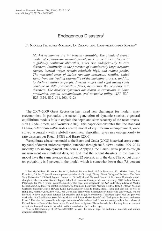
Implicitly in our calibration, we assume the same matching technology within and outside disasters. Figure 1 plots the long-term US Beveridge curve from April 1929 to December 2013. Most important, the 1929–1939 observations, as well as the 1940–1950 observations, form a natural extension of the postwar Beveridge curve into the high-unemployment-low-vacancy and low-unemployment-high-vacancy regions, respectively. We interpret the evidence as indicating the stability of the underlying matching technology over the past eight-and-a-half decades. In particu-lar, the Great Depression was not associated with any visible shift in the Beveridge curve. Finally, the vacancy rate experienced large declines during the Great Depression, consistent with our model. The vacancy rate dropped from 2 percent in September 1929 to 0.44 percent in March 1933, representing a steep decline of 78 percent (the online Appendix).


Basic Moments.—From the baseline model’s stationary distribution (after 6,000 burn-in months), we repeatedly simulate 10,000 samples, each with 1,836 months. On each sample, we time-aggregate the monthly output into 153 annual observa-tions and the first 1,656 monthly consumption observations into 138 annual obser-vations. Time-aggregation means that we add up 12 monthly observations within a given year, and treat the sum as the year’s annual observation. The sample lengths match the cross-country average sample lengths in Tables 1 and 2. We then calculate the annual volatilities, skewness, kurtosis, and autocorrelations of log consumption and output growth. For each moment, we report the mean as well as the 5th and 95th percentiles across the 10,000 simulations. We also report p-values that are the frequencies with which a given model moment is larger than its data counterpart.

Table 3 shows that the output volatility is 5.3 percent per annum in the model, which is close to the data moment, 5.6 percent. The consumption volatility of 4.7 percent in the model is smaller than 6.4 percent in the data. Both output and con-sumption growth rates are somewhat negatively skewed in the data, with coefficients of − 1 and − 0.6 , respectively. However, the output and consumption growth rates in the model are slightly positively skewed with a coefficient about 0.9. The model

0 5 10 15 20 25 30

Unemployment rate (in percent)

0

1

2

3

4

5

6

Vac

ancy

rat

e (in

per

cent

)

Figure 1. The US Beveridge Curve, April 1929–December 2013

Notes: The April 1929–December 1939 observations are in red circles, the January 1940–December 1950 observa-tions are in black diamonds, and the remaining observations are in blue squares.Source: The unemployment and vacancy rate series from Petrosky-Nadeau and Zhang (2013)


matches the leptokurtic distributions of output and consumption growth in the data. The kurtosis of the output growth is 11.9, and that of the consumption growth 9.2 in the data. The corresponding model moments are 12.8 and 14.4, respectively. Finally, consistent with the data, both output and consumption growth rates are positively autocorrelated at the first lag, but not autocorrelated at longer lags.

From panel C, the mean unemployment rate is 6.3 percent in the model, which is not far from 7.1 percent in the data. The model also reproduces positively skewed and leptokurtic unemployment rates, with skewness and kurtosis 3.5 and 19.2, and the data moments of 2 and 6.8, respectively, are within the model’s 90 percent confidence interval. To compute the unemployment volatility, we take quarterly averages of monthly unemployment rates, and detrend with Hodrick-Prescott (1997, HP) filtered proportional deviations from the mean. The unem-ployment volatility is 23.4 percent in the model, which is not far from 19.8 percent in the data. The model also implies an unemployment-vacancy correlation of − 0.5 ( − 0.7 in the data).

Table 3—Basic Moments in the Baseline Model

Data Mean 5 percentile 95 percentile p-value

Panel A. Output growth σ Y 5.63 5.31 2.90 11.56 0.31 S Y −1.02 0.85 −0.39 3.35 0.99 K Y 11.87 12.8 3.08 34.99 0.41 ρ 1 Y 0.16 0.24 0.01 0.63 0.58 ρ 2 Y 0 −0.11 −0.31 0.23 0.16 ρ 3 Y 0.02 −0.12 −0.32 0.08 0.1 ρ 4 Y −0.02 −0.11 −0.31 0.08 0.23

Panel B. Consumption growth σ C 6.37 4.65 2.12 11.26 0.21 S C −0.55 0.91 −0.50 3.57 0.96 K C 9.19 14.4 3.16 38.59 0.54 ρ 1 C 0.07 0.23 −0.02 0.65 0.79 ρ 2 C 0.03 −0.12 −0.33 0.24 0.14 ρ 3 C 0 −0.12 −0.34 0.09 0.15 ρ 4 C −0.02 −0.11 −0.32 0.09 0.23

Panel C. Unemployment rate E[U ] 7.12 6.28 4.83 10.54 0.18 σ U 19.83 23.41 5.45 53.49 0.48 S U 1.99 3.52 1.49 5.82 0.86 K U 6.82 19.18 5.24 41.78 0.89

Notes: For each moment, this table reports the mean as well as the 5 and 95 percentiles across the simulations. The p-values are the percentages with which a given model moment is larger than its data counterpart. σ Y and σ C denote volatilities, S Y and S C skewness, K Y and K C kurtosis, and ρ i

Y and ρ i C the ith-order autocorrelations of log output and consumption growth rates, respec-

tively. E[U], S U , and K U are the mean, skewness, and kurtosis of the monthly unemployment rate, respectively, and σ U is its quarterly volatility. We take quarterly averages of monthly unemploy-ment rates, and detrend the quarterly series as HP-filtered proportional deviations from the mean with a smoothing parameter of 1,600. σ Y , σ C , E [U] , and σ U are in percent. Sources: The output and consumption data moments are based on the Barro-Ursúa (2008) histor-ical cross-country panel, extended through 2013, and the unemployment data moments are based on the Petrosky-Nadeau-Zhang (2013) US series from April 1929 to December 2013. The model moments are based on authors’ calculations from 10,000 simulated samples.


C. Endogenous Disasters

Most important, the baseline economy gives rise to endogenous disasters.

Quantitative Results.—We simulate one million months from the model, and report the empirical cumulative distribution functions for unemployment, output, and consumption. Figure 2 shows that unemployment is positively skewed with a long right tail. The mean unemployment rate is 6.2 percent, and the median 4.9 per-cent. The 2.5th percentile of the unemployment rate, 4.3 percent, is close to the median, whereas the 97.5th percentile is far away, 17 percent. As a mirror image, employment is negatively skewed with a long left tail. Consequently, output and consumption both exhibit rare but deep disasters. With small probabilities, the econ-omy falls off a cliff.5

5 The sharp drops in output and consumption levels in Figure 2 are consistent with the slightly positive skewness of output and consumption growth rates in Tables 1 and 2. The extreme left tails in the levels give rise to large sub-sequent growth rates, as their denominators become small. In the extended model with capital (Section IIB), the left

Panel A. Unemployment rate

0 00.2 0.4 0.6 0.8 10

0.2

0.4

0.6

0.8

1

Unemployment

Pro

babi

lity

Panel B. Output

0.5 1 1.50

0.2

0.4

0.6

0.8

1

Output

Pro

babi

lity

0 0.5 1 1.50

0.2

0.4

0.6

0.8

1

Consumption

Pro

babi

lity

Panel C. Consumption

Figure 2. Empirical Cumulative Distribution Functions: The Baseline Model

Note: Results are based on one million months simulated from the baseline model.Source: Authors’ calculations


Do the rare disasters arising endogenously from the model resemble those in the data? Barro and Ursúa (2008) apply a peak-to-trough method on their cross-country panel to identify rare disasters, which are defined as cumulative fractional declines in per capita consumption or output of at least 10 percent. Suppose there are two states, normalcy and disaster. The disaster probability measures the likelihood with which the economy shifts from normalcy to disaster in a given year. The number of disaster years is the number of years in the interval between peak and trough for each disaster event. The number of normalcy years is the total number of years in the sample minus the number of disaster years. The disaster probability is calculated as the ratio of the number of disasters divided by the number of normalcy years. For each disaster event, the disaster size is the cumulative fractional decline in per capita output or consumption from peak to trough, and the disaster duration is the number of years from peak to trough.6

We apply the peak-to-trough method on the extended cross-country panel. Table 4 shows the estimates. For output, the disaster probability is 7.8 percent, the average size of disasters 22 percent, and the average duration 3.7 years. For consumption, the disaster probability is 8.6 percent, the average size 23.2 percent, and the duration 3.8 years. Our disaster probability estimates, 7.8 percent and 8.6 percent for output and consumption, are higher than those in Barro and Ursúa, 3.7 percent and 3.6 per-cent, respectively. The crux is that we adjust for trend growth in the data to be con-sistent with our model with no growth. In particular, we subtract each observation of log annual output growth with its mean of 1.8 percent per annum, and subtract each observation of log annual consumption growth with its mean of 1.7 percent in the historical cross-country panel. Ignoring trend growth in our extended sample yields the disaster probabilities of 3.5 percent for output and 4.2 percent for consumption, which are close to Barro and Ursúa’s estimates. The average size and duration esti-mates are relatively unaffected. Clearly, adjusting for trend growth in the data raises the hurdle for the model.

We simulate 10,000 artificial samples from the model’s stationary distribution, each with 1,836 months. On each sample, we time-aggregate monthly output and consumption into annual observations, and then apply the Barro-Ursúa peak-to-trough measurement. Table 4 shows that the output disaster probability in the model is 5 percent, which is lower than 7.8 percent in the data, but the data moment is within two standard deviations from the model ( p-value = 0.09). The average disas-ter size in the model, 22.2 percent, is close to the data moment, 22 percent. The average duration in the model of 4.4 years is also close to 3.7 years in the data. For consumption disasters, the probability is only 2.9 percent in the model, which is substantially lower than 8.6 percent in the data ( p-value = 0). The average disaster size is 25.6 percent in the model, which is close to 23.2 percent in the data. The average duration is 4.9 years, which is not far from 3.8 years in the data. Finally, Figure 3 reports the frequency distributions of output and consumption disasters

tails are less extreme because of the buffeting effect of capital. As a result, the skewness of output and consumption growth rates is only 0.1, albeit still positive.

6 In continuous time models, disasters are often modeled as jumps in consumption growth. If reformulated in continuous time, disasters in our model would arise from time-varying drift and diffusion of output and consump-tion growth. However, jumps are only a convenient modeling device in continuous time. In the data and in discrete time models, disasters arising from these different sources are observationally equivalent.


by size and duration simulated from the model. The size and duration distributions display similar patterns as those in the data (Barro and Ursúa 2008, Figures 1 and 2). In particular, the size distributions seem to follow a power-law density.7

Comparative Statics.—To shed light on the intuition behind the model’s disaster dynamics, we conduct six comparative statics. (i, ii) We reduce the flow value of unemployment, b , from 0.85 in the benchmark calibration to 0.825, and then to 0.4. Because of its importance, we consider two alternative values of b . (iii) We lower the job separation rate, s , from 0.04 to 0.035. (iv) We adjust the unit costs of vacancy from κ t = 0.5 + 0.5q( θ t ) to κ t = 0.7 , with κ 0 = 0.7 and κ 1 = 0 (the average κ t is 0.7 under the benchmark calibration). (v) We reduce the curvature of the matching function, ι , from 1.25 to 1.1. Finally, (vi) we raise the workers’ bargaining power, η , from 0.04 to 0.05. In each experiment, all the other parameters remain unchanged.

Table 5 reports the results. With b = 0.825 , the output disaster probability reduces from 5 to 3.6 percent, and the consumption disaster probability from 2.9 to 1.6 percent. The average disaster size is lowered from 22.2 to 16.1 percent for output, and from 25.6 to 16.3 percent for consumption. The average duration of disasters increases slightly. The output and consumption volatilities drop to 3.4 and 2.6 percent, and the mean and volatility of the unemployment rate fall to 5 and 11 percent, respectively. With b = 0.4 , the disaster probability falls further to 2.5 percent for output and 1.3 percent for consumption. The average size drops to 13.4 and 12.4 percent, respectively. The low value of b implies low wages and an

7 In the online Appendix, we have worked out a model with leisure in the utility function, log ( C t + h U t ) , in which h > 0 is a constant parameter. With b = 0.5 and h = 0.35 , while keeping all other parameter values unchanged, the results, including the disaster moments, are quantitatively close to those from the baseline model.

Table 4—Disaster Moments

Model

Data Mean 5 percentile 95 percentile p-value

Panel A. OutputProbability 7.83 5.04 2.24 8.57 0.09Size 21.99 22.22 12.7 46.24 0.33Duration 3.72 4.44 3.2 6 0.79

Panel B. ConsumptionProbability 8.57 2.86 0.71 5.83 0.00Size 23.16 25.64 11.26 62.13 0.36Duration 3.75 4.91 3 7 0.81

Notes: On each artificial sample, we time-aggregate output and consumption into annual observations, and apply the peak-to-trough method to identify disasters as cumulative fractional declines in output or consumption of at least 10 percent. We report the averages, 5 and 95 percentiles, and p-values across the simulations. If no disaster appears in a given sample, we set its disaster probability to be 0, and the probability mean and percentiles are calcu-lated across all 10,000 samples, each with 1,836 months. However, disaster size and duration are calculated across samples with at least one disaster. The disaster probabilities and average size are in percent, and the average dura-tion is in terms of years.Sources: The data moments are estimated from applying the Barro-Ursúa (2008) peak-to-trough method on their cross-country panel, extended through 2013. We adjust for trend growth in the data. The model moments are obtained from authors’ calculations based on 10,000 simulations.


exceedingly high profits-to-output ratio of 31 percent. The mean unemployment rate falls to 4 percent, and the unemployment volatility to only 0.14 percent. However, the presence of disaster dynamics with b = 0.4 implies that disasters are even more robust to changes in b than the unemployment volatility.

Intuitively, equation (10) shows that with small profits, wages are inertial with respect to productivity shocks. When productivity is low, wages remain high, shrink-ing the small profits to stifle job creation flows. In contrast, with large profits, wages are sensitive to shocks. With b = 0.4 , the wage elasticity to productivity increases to 0.66 from 0.51 with b = 0.85 . As such, when productivity is low, employment falls, but wages drop as well, providing hiring incentives for the firm to counteract job destruction flows. Consequently, disaster dynamics are dampened.

In the third experiment, reducing the separation rate lowers disaster probabili-ties and size. With s = 0.035 , the disaster probability is 4.4 percent for output and 2.4 percent for consumption, both of which are still substantial. The disaster size declines somewhat, and the duration rises slightly. Intuitively, because jobs are destroyed at a lower rate, the economy can create enough jobs to shore up employ-ment in time to reduce disaster risk.

Panel A. Output disasters by size Panel B. Consumption disasters by size

0 0.2 0.4 0.6 0.8 10

1

2

3

4

5

Num

ber

of d

isas

ters

Cumulative decline

0 0.2 0.4 0.6 0.8 10

1

2

3

4

5

Num

ber

of d

isas

ters

Cumulative decline

Panel C. Output disasters by duration Panel D. Consumption disasters by duration

1 2 3 4 5 6 7 8 9 100

0.5

1

1.5

Num

ber

of d

isas

ters

0

0.5

1

1.5N

umbe

r of

dis

aste

rs

Duration1 2 3 4 5 6 7 8 9 10

Duration

Figure 3. Distributions of Output and Consumption Disasters by Size and Duration from the Baseline Model

Note: Results are based on 10,000 simulations, each with 1,836 months.Source: Authors’ calculations


Without the fixed costs of vacancy, the disaster probability drops from 5 to 4.1 per-cent for output, and from 2.9 to 1.9 percent for consumption. The disaster size falls from 22.2 to 18.2 percent for output, and from 25.6 to 20.2 percent for consumption. The output and consumption volatilities decline to 4.1 and 3.3 percent, respectively. The mean unemployment rate falls from 6.3 to 5.5 percent, and its volatility from 23 to 15 percent. While Pissarides (2009) shows the impact of fixed costs on the unemployment volatility, we quantify the important impact on disaster dynamics.

Reducing the curvature of the matching function, ι , from 1.25 to 1.1 raises the disaster probability somewhat to 5.3 percent for output and 3 percent for consump-tion. The disaster size and duration, as well as output, consumption, and unem-ployment volatilities all remain relatively unchanged. The mean unemployment rate increases to 6.7 percent. Intuitively, a lower curvature of the matching function means that the labor market is more frictional in matching vacancies with unem-ployed workers. Because job creation flows are hampered, whereas job destruction flows remain unchanged, the lower curvature raises the unemployment rate, and strengthens somewhat the disaster dynamics.

Finally, increasing the workers’ bargaining weight, η , from 0.04 to 0.05 raises the disaster probability to 5.6 percent for output and 3.6 percent for consumption. As workers gain more bargaining power, the mean unemployment rate rises to 6.8 per-cent, the output volatility to 5.6 percent, and the consumption volatility 5 percent. However, the unemployment volatility is barely changed.

Downward Rigidity in the Marginal Costs of Hiring.—In addition to wage inertia, the other key determinant of the firm’s hiring decisions is the marginal costs of hir-ing, κ 0 / q( θ t ) + κ 1 . To illustrate the properties of the marginal costs, Figure 4 plots the vacancy filling rate, q( θ t ) , as well as the marginal costs of hiring in the model with small profits ( b = 0.85 ) and with large profits ( b = 0.4 ). Each panel has three lines, each corresponding to a different level of productivity.

Table 5—Comparative Statics for the Disaster Moments in the Baseline Model

Benchmark b = 0.825 b = 0.4 s = 0.035 κ t = 0.7 ι = 1.1 η = 0.05

Panel A. OutputProbability 5.04 3.61 2.53 4.42 4.05 5.29 5.57Size 22.22 16.07 13.41 19.87 18.2 21.97 22.69Duration 4.44 4.57 4.7 4.5 4.51 4.41 4.4

Panel B. ConsumptionProbability 2.86 1.62 1.32 2.43 1.85 3.04 3.59Size 25.64 16.31 12.35 22.25 20.19 25.05 25.21Duration 4.91 5.19 5.2 4.97 5.1 4.88 4.78

Notes: The first column reports the disaster moments from the benchmark calibration (Table 4), and the other col-umns show six comparative statics: (i, ii) b = 0.825 and b = 0.4 are for the flow value of unemployment set to 0.825 and 0.4, respectively; (iii) s = 0.035 is for the job separation rate set to 0.035; (iv) κ t = 0.7 is for the propor-tional unit costs of vacancy κ 0 = 0.7 and the fixed unit costs κ 1 = 0; (v) ι = 1.1 is for the curvature of the matching function set to 1.1; and (vi) η = 0.05 is for the workers’ bargaining weight set to 0.05. In each experiment, all the other parameters are identical to those in the benchmark calibration.Source: Authors’ calculations based on 10,000 simulations, each with 1,836 months


Panel A shows that when productivity is low, the vacancy filling rate, q( θ t ) , is essentially unity with b = 0.85 . Intuitively, the labor market is populated by a large number of unemployed workers competing for a few vacancies. Filling a vacancy with an unemployed worker is guaranteed, with no room for the vacancy filling rate to increase further. Accordingly, the marginal costs of hiring equal the constant κ 0 + κ 1 , with no room to drop further, giving rise to the downward rigidity in the marginal costs (panel B). The rigid marginal costs suppress the firm’s hiring incen-tives, smothering job creation flows and giving rise to disasters.

Arising from the trading externality of the matching process, this downward rigidity subsists even without the fixed costs of vacancy ( κ 1 = 0 ). By putting the constant κ 1 into the marginal costs of hiring, the fixed costs further restrict the abil-ity of the marginal costs to decline, fortifying the downward rigidity. This economic

Panel A. The vacancy �lling rate,small pro�ts (b = 0.85)

Panel B. The marginal costs of hiring, small pro�ts (b = 0.85)

0 0.2 0.4 0.6 0.8 1 10

0.2

0.4

0.6

0.8

1

Employment Employment

Employment Employment

0 0.2 0.4 0.6 0.81

2

3

4

5

Panel C. The vacancy �lling rate,large pro�ts (b = 0.4)

Panel D. The marginal costs of hiring, large pro�ts (b = 0.4)

0.2 0.4 0.6 0.8 10

0.2

0.4

0.6

0.8

1

0.2 0.4 0.6 0.8 10

2

4

6

8

10

12

Figure 4. The Vacancy Filling Rate and the Marginal Costs of Hiring in the Baseline Model: Small and Large Profits

Notes: Let x 1 < x 2 < ⋯ < x 17 denote the x grid. In each panel, the blue solid line is for x t = x 3 , the red dashed line for x t = x 9 , and the black dashed-dotted line for x t = x 15 . b is the flow value of unemployment.Source: Authors’ calculations


mechanism explains why removing the fixed costs makes disasters less frequent and less severe in the baseline model (Table 5).

Panels C and D show that the downward rigidity in the marginal costs is absent with large profits. The vacancy filling rate, q( θ t ) , is quite sensitive to employment when profits are large (panel C). Intuitively, with b = 0.4 , vacancies are plentiful even when productivity is low. The labor market is populated by a fair number of both vacancies and unemployed workers. As employment falls, q( θ t ) keeps climb-ing, reducing the marginal costs of hiring (panel D). The falling marginal costs stimulate job creation flows, dampening disaster dynamics.

Which Disasters?—The baseline model is a textbook economic model, yet we opt to explain disaster moments from the Barro-Ursúa (2008) dataset. The dataset contains not only economic disasters such as the Great Depression, but also wars and natural disasters such as earthquakes, floods, and epidemics. Our choice merits further discussion.

First, we calibrate the volatility of productivity shocks, σ , to match the output volatility in the data. Because wars and natural disasters are exogenous to the model economy, these impulses can at least in principle be captured by large negative pro-ductivity shocks. The model then quantifies the impact of these impulses on endog-enous variables such as unemployment and output. As noted, even for the Great Depression, the model does not identify its origins.

Second, disentangling economic disasters empirically from other types of disasters requires judgment calls that are likely arbitrary. Wars could be endoge-nous responses to harsh economic conditions, which give rise to destructive con-flicts among rival nations. Conversely, the Great Depression has been argued to originate from the First World War. Temin (1989, p. 1) writes: “The origins of the Great Depression lie largely in the disruptions of the First World War. Its spread owes much to the hostilities and continuing conflicts that were created by the war and the Treaty of Versailles. And its effects—particularly the vic-tory of National Socialism in Germany—clearly extend to the Second World War.” Third, to the extent that wars also propogate shocks, the Barro-Ursúa (2008) disaster moments pose a very high hurdle for any economic model to explain.

We have also experimented with an alternative calibration. Instead of matching the output volatility of 5.6 percent per annum in the cross-country panel, we rescale the volatility of productivity shocks, σ , to match the output volatility of 4.3 percent in the historical 1790–2013 US sample. This target is conservative because it is even lower than 4.9 percent in the 1929–2013 US sample. We target the US data because the damage from world wars on its economy is negligible compared with other nations. Specifically, we set σ = 0.00925 , which implies a volatility of 4.3 percent for output and 3.6 percent for consumption in the baseline model. The unemploy-ment rate is 5.8 percent on average, and its volatility 18.7 percent. More important, disaster dynamics remain substantial. The disaster probability is 4 percent, size 19.6 percent, and duration 4.6 years for output, and 2.1 percent, 22.3 percent, and 5 years, respectively, for consumption. As such, the endogenous disasters in the model are relatively robust to the large σ value required to match the output volatility of 5.6 percent in the Barro-Ursúa (2008) cross-country panel.


II. Extensions

The disaster dynamics are robust to several extensions to the baseline model.

A. Home Production

In this subsection, we extend the baseline model to incorporate home production (Benhabib, Rogerson, and Wright 1991). The household derives utility not only from the consumption of market goods, C mt , but also from the consumption of non-market, home-produced goods, C ht . We define the composite consumption bundle as

(12) C t ≡ [a C mt e + (1 − a) C ht e ] 1/e ,

in which e ∈ (0, 1] and a ∈ [0, 1] . The elasticity of substitution between market and nonmarket goods is 1/(1 − e) , and a is the relative weight of market goods over nonmarket goods. The household has log utility over the composite consumption, log ( C t ) . The marginal utility of the market consumption is ϕ t ≡ a C mt e−1 / C t e , and the stochastic discount factor is

(13) M t+1 ≡ β ϕ t+1 _ ϕ t = β ( C mt+1 _ C mt )

e−1

( C t _ C t+1 )

e

.

The home production technology is given by

(14) C ht = X h U t ,

in which X h > 0 is a constant parameter. This technology is nonstochastic. For instance, Aguiar, Hurst, and Karabarbounis (2013) find no evidence that indicates shocks to home production. Let z t denote the total flow value of unemployment,

(15) z t ≡ X h ( 1 − a _ a ) ( C mt _ C ht )

1−e

+ b.

As shown in the online Appendix, the equilibrium Nash-wage becomes

(16) W t = η( X t + κ t θ t ) + (1 − η) z t .

The market-clearing condition becomes C mt + κ t V t = X t N t . The rest of the model remains identical to the baseline model.

We set the value of b to 0.5, which is the flow value of unemployment other than home production, such as unemployment insurance, disutility of work, and leisure. In the absence of concrete evidence on home technology, we set its productivity parameter, X h , to be unity, which is the long-term mean of the market technology. We next calibrate the volatility of market productivity, σ , the relative weight of the


market goods, a , and the parameter governing the elasticity between market and home consumption, e , to match three data moments, including the output volatility, as well as the mean and volatility of unemployment. To facilitate comparison, all the other parameter values remain identical to the baseline model.

This procedure yields σ = 0.014 , a = 0.8 , and e = 0.85 . Table 6 reports the results. Together, these parameter values imply an output volatility of 5.3 percent. The mean unemployment rate is 6.6 percent, and its volatility 19.5 percent, which is close to 19.8 percent in the data. The market consumption volatility is 4.7 percent,

Table 6—Quantitative Results: The Home Production Model

Data Model

σ 0.01 0.014 0.014 0.014 a 0.8 0.8 0.8 0.85 e 0.85 0.85 0.9 0.85

Panel A. Output growth σ Y 5.63 3.41 5.29 4.62 3.9 S Y − 1.02 0.06 0.15 0.13 0.01 K Y 11.87 3.83 4.92 4.95 3.42 ρ 1 Y 0.16 0.15 0.16 0.15 0.14 ρ 2 Y 0 − 0.13 − 0.13 − 0.13 − 0.12 ρ 3 Y 0.02 − 0.1 − 0.11 − 0.1 − 0.1 ρ 4 Y − 0.02 − 0.08 − 0.08 − 0.08 − 0.08 Prob Y 7.83 5 9.95 8.2 6.88Size Y 21.99 15 18.58 17.21 15.43Dur Y 3.74 4.32 3.74 3.88 3.98

Panel B. Consumption growth σ C 6.37 2.91 4.67 3.74 2.9 S C − 0.55 0.09 0.2 0.2 0.03 K C 9.19 4.22 5.73 5.97 3.48 ρ 1 C 0.07 0.15 0.16 0.15 0.14 ρ 2 C 0.03 − 0.13 − 0.14 − 0.14 − 0.12 ρ 3 C 0 − 0.1 − 0.11 − 0.11 − 0.1 ρ 4 C − 0.02 − 0.08 − 0.09 − 0.08 − 0.08 Prob C 8.57 3.35 7.52 4.95 3.43Size C 23.16 14.42 18.06 16.34 13.81Dur C 3.75 4.65 3.99 4.31 4.59

Panel C. Unemployment rate E[U] 7.12 5.97 6.58 5.33 4.5 σ U 19.83 10.75 19.53 15.3 4.07 S U 1.99 1.86 2.44 3.06 2.1 K U 6.82 7.48 10.42 15.73 9.87

Notes: σ is the conditional volatility of the log productivity shocks to the market goods technology, a the relative weight of market goods over nonmarket goods, and 1/(1 − e) the elasticity of substitution between market and non-market goods. σ Y and σ C are the volatilities, S Y and S C skewness, K Y and K C kurtosis, and ρ i

Y and ρ i C the ith-order

autocorrelations of log output and consumption growth rates, respectively. Prob Y , Size Y , and Dur Y , as well as Prob C , Size C , and Dur C are the probability, size, and duration of output and consumption disasters, respectively. E[U], S U , and K U are the mean, skewness, and kurtosis of the monthly unemployment rate, respectively, and σ U is its quarterly volatility. σ Y , σ C , E [U] , and σ U are in percent. Sources: The output and consumption data moments are based on the Barro-Ursúa (2008) historical cross-coun-try panel, extended through 2013, and the unemployment data moments are based on the Petrosky-Nadeau-Zhang (2013) US series from April 1929 to December 2013. The model moments are based on authors’ calculations from 10,000 simulated samples.


which is identical to that in the baseline model. The model also reproduces the pos-itively skewed and leptokurtic unemployment rate distribution.

More important, disaster dynamics are robust to home production. The disaster probability is 10 percent for output, which is even higher than 7.8 percent in the data and 5 percent in the baseline model. The probability is 7.5 percent for consumption, which is lower than 8.6 percent in the data, but higher than 2.9 percent in the baseline model. However, the disaster size is smaller, 18.6 percent for output and 18.1 per-cent for consumption. The disaster duration is close to the data, 3.7 years for output and 4 for consumption.

Table 6 also reports three comparative statics. First, not surprisingly, reducing the volatility of productivity shocks from 0.014 to 0.01, which is the value in the base-line model, lowers the output volatility to 3.4 percent. The mean unemployment rate falls to 6 percent, and its volatility to 10.8 percent. Even with σ = 0.01 , the disaster probability is still 5 percent for output and 3.4 percent for consumption. However, the disaster size is smaller, 15 percent for output, and 14.4 percent for consumption. Finally, the duration rises to 4.3 years for output and 4.7 for consumption.8

Increasing the e parameter governing the elasticity of substitution between mar-ket and home goods from 0.85 to 0.9 weakens disaster dynamics. Both the disaster probability and size decrease, and duration increases. The mean unemployment rate falls from 6.6 to 5.3 percent, and volatility from 19.5 to 15.3 percent. The market consumption dominates the home consumption in magnitude ( C mt / C ht is 15.4 on average). As e increases, equation (15) implies that the flow value of unemployment, z t , falls. Intuitively, a higher e means that the two types of consumption become more substitutable, and the home consumption loses its relative appeal, despite its small size. As such, z t falls from 0.87 to 0.83 on average, reducing unemployment and its volatility, and dampening disaster dynamics.

Increasing the relative weight of market goods, a , from 0.8 to 0.85 also damp-ens the disaster dynamics. The disaster probability falls from 10 to 6.9 percent for output, and the disaster size from 18.6 to 15.4 percent. More drastically, the mean unemployment rate falls from 6.6 to 4.5 percent, and its volatility from 19.5 to only 4.1 percent. As a increases, equation (15) implies that the flow value of unemploy-ment, z t , falls. Intuitively, as the relative weight of market goods increases in the utility function, home goods become less valuable to the household. As a result, z t falls from on average 0.87 to 0.77, which greatly reduces unemployment and its volatility, weakening disaster dynamics.

Our calibration is parsimonious in that, to facilitate comparison, all parameters except for the volatility of productivity shocks, σ , are identical to those in the base-line model. In particular, this strategy yields e = 0.85 , which implies an elasticity of 6.67 between market and home goods. This e value is not far from 0.8 calibrated in Benhabib, Rogerson, and Wright (1991), but is higher than the estimates in Rupert, Rogerson, and Wright (1995, Table 4) based on microdata, ranging from 0.36 to 0.75. However, comparative statics show that, all else equal, increasing e to 0.9

8 Rescaling σ to 0.012 matches the output volatility of 4.3 percent in the 1790–2013 US sample. The mean unemployment rate falls to 6.2 percent, and the unemployment volatility 14.8 percent. The disaster dynamics remain substantial. The disaster probability is 7.5 percent, size 16.7 percent, and duration 4 years for output, and the probability 5.4 percent, size 16.1 percent, and duration 4.3 years for consumption.


dampens disaster dynamics. As such, alternative calibrations with a lower value of e are likely to strengthen the disasters in the model.

B. Capital

In this subsection, we augment the baseline model in Section I with capital, which is standard in the business cycle literature (Kydland and Prescott 1982). The firm uses labor, N t , and capital, K t , to produce with a constant return of scale technology,

(17) Y t = X t K t α N t 1−α ,

in which Y t is output, and α ∈ (0, 1) is the capital’s weight. We specify x t = log ( X t ) as

(18) x t+1 = (1 − ρ) x ̅ + ρ x t + σ ϵ t+1 ,

in which x ̅ is the unconditional mean of x t . We rescale x ̅ to make the average mar-ginal product of labor around unity to ease comparison with the baseline model.

The firm incurs adjustment costs when investing. Capital accumulates as

(19) K t+1 = (1 − δ) K t + Φ( I t , K t ) ,

in which δ is the capital depreciation rate, I t is investment, and

(20) Φ( I t , K t ) ≡ [ a 1 + a 2 _ 1 − 1/ ν ( I t _ K t

) 1−1/ν

] K t

is the installation function with the supply elasticity of capital ν > 0 . We set a 1 = δ/(1 − ν) and a 2 = δ 1/ν to ensure no adjustment costs in the deterministic steady state (Jermann 1998).

The investment Euler equation is given by

(21) 1 _ a 2 ( I t _ K t

) 1/ν

= E t [ M t+1 (α Y t+1 _ K t+1

+ 1 _ a 2 ( I t+1 _ K t+1

) 1/ν

(1 − δ + a 1 ) + 1 _ ν − 1 I t+1 _ K t+1

) ] ,

and the intertemporal job creation condition becomes

(22) κ 0 _ q( θ t )

+ κ 1 − λ t = E t [ M t+1 ((1 − α) Y t+1 _ N t+1 − W t+1 + (1 − s) ( κ 0 _

q( θ t+1 ) + κ 1 − λ t+1 ) ) ] .

The equilibrium wage, W t , which the firm takes as given, follows

(23) W t = η [(1 − α) Y t _ N t + κ t θ t ] + (1 − η ) b.

The goods market-clearing condition becomes C t + I t + κ t V t = Y t . Finally, the extended model with capital is more challenging to solve than the baseline model.


Capital, K t , becomes a new state variable in addition to x t and N t . Also, the invest-ment Euler equation (21) must be solved together with the intertemporal job cre-ation condition (22).

We set the capital’s weight in production, α , to 1/3, and the depreciation rate, δ , to 0.01. We calibrate the unconditional mean of log productivity, x ̅ = − 0.771 , to make the long-term average of the marginal product of labor, (1 − α) Y t / N t , around 1 in simulations. For the capital elasticity, ν , we vary it from 0.5 to 2, covering a wide range of empirically plausible values. To facilitate comparison, all the other parameter values are identical to those in the baseline model.

With capital added to the baseline model, the model column with σ = 0.01 (and ν = 2 ) in Table 7 shows the smoothing effect of investment. The output volatility drops to 3.4 percent, and the consumption volatility to 2.4 percent. The mean unem-ployment rate falls to 6 percent, and volatility to 14 percent. The disaster probabili-ties and size, as well as the skewness and kurtosis of output and consumption growth all decline. Specifically, the output disaster size falls to 15.8 percent, but its disaster probability drops only slightly to 4.6 percent, which remains substantial.

We rescale the conditional volatility of productivity shocks, σ , to 0.014 to obtain an output volatility of 5.1 percent (with ν = 2 ), which is close to 5.3 percent in the baseline model. The consumption volatility is 3.7 percent, which is lower than 4.7 percent in the baseline model. The mean unemployment rate is 7.5 percent, and its volatility 22.5 percent. The investment growth volatility is 7 percent, which, although much lower than 23.3 percent in the 1929–2013 US sample, is not far from 8.9 percent from 1951 onward. Because a historical cross-country panel of invest-ment is unavailable, we do not estimate disaster moments for investment. As in the data, investment growth in the model is positively autocorrelated at the first lag, but negatively autocorrelated at longer lags.

Most important, disaster dynamics are robust to the inclusion of capital. The disas-ter probability is 9.5 percent for output, which is somewhat higher than 7.8 percent in the data. The disaster probability is 5.3 percent for consumption, which is still lower than 8.6 percent in the data. However, the disaster size is smaller, 19 percent for output versus 22 percent in the data, and 17.7 percent for consumption versus 23.2 percent in the data. The disaster duration is somewhat higher than those in the data.9

The rest of the model columns in Table 7 examines the impact of the supply elas-ticity of capital, ν , on the quantitative results. Reducing ν from 2 to 1.5 and further to 0.5 dampens investment dynamics, but amplifies consumption dynamics. The investment volatility drops from 7 to 6.1 and further to 2.9 percent, whereas the con-sumption volatility rises from 3.7 to 4 and further to 4.8 percent. The consumption disaster probability goes up from 5.3 to 6 and further to 8.2 percent, the disaster size increases slightly, and duration decreases slightly. Intuitively, ν governs the magni-tude of capital adjustment costs. A falling ν means rising adjustment costs, which dampen investment dynamics, but amplify consumption dynamics. Finally, varying ν shows only weak impact on output and unemployment dynamics. As ν falls from

9 Rescaling the volatility of productivity shocks, σ , to 0.012 implies an output volatility of 4.3 percent, which equals that in the 1790–2013 US sample. The consumption volatility is 3.1 percent, and the investment volatility 5.9 percent. The mean unemployment rate is 6.8 percent, and the unemployment volatility 18.8 percent. The disaster dynamics remain substantial. The disaster probability is 7.2 percent, size 17.5 percent, and duration 4.2 years for output, and the disaster probability is 3.7 percent, size 16.3 percent, and duration 4.8 years for consumption.


2 to 0.5, the output volatility falls from 5.1 slightly to 4.9 percent, the disaster prob-ability from 9.5 to 9.1 percent, and the disaster size and duration are unaffected. The mean unemployment rate falls from 7.5 to 6.9 percent, but its volatility, skewness, and kurtosis are unchanged.

Table 7—Quantitative Results: The Capital Model

Data Model

σ 0.01 0.014 0.014 0.014 ν 2 2 1.5 0.5

Panel A. Output growth σ Y 5.63 3.35 5.11 5.1 4.93 S Y − 1.02 0.1 0.12 0.11 0.1 K Y 11.87 4.11 4.5 4.49 4.34 ρ 1 Y 0.16 0.18 0.19 0.19 0.17 ρ 2 Y 0 − 0.1 − 0.09 − 0.1 − 0.12 ρ 3 Y 0.02 − 0.08 − 0.07 − 0.08 − 0.09 ρ 4 Y − 0.02 − 0.07 − 0.06 − 0.07 − 0.08 Prob Y 7.83 4.55 9.45 9.4 9.07Size Y 21.99 15.76 18.97 18.81 18.08Dur Y 3.72 4.58 3.89 3.87 3.8

Panel B. Consumption growth σ C 6.37 2.38 3.74 4 4.75 S C − 0.55 0.08 0.12 0.14 0.17 K C 9.19 4.67 5.18 5.1 4.79 ρ 1 C 0.07 0.21 0.22 0.2 0.17 ρ 2 C 0.03 − 0.08 − 0.07 − 0.09 − 0.12 ρ 3 C 0 − 0.07 − 0.06 − 0.08 − 0.09 ρ 4 C − 0.02 − 0.06 − 0.06 − 0.06 − 0.08 Prob C 8.57 2.08 5.31 5.95 8.18Size C 23.16 14.9 17.69 17.68 17.98Dur C 3.75 5.39 4.51 4.33 3.9

Panel C. Investment growth σ I 23.33 4.52 6.98 6.06 2.88 S I − 0.79 0.2 0.2 0.17 0 K I 8.72 4.51 4.94 4.92 4.66 ρ 1 I 0.22 0.17 0.17 0.18 0.19 ρ 2 I − 0.04 − 0.12 − 0.12 − 0.11 − 0.1 ρ 3 I − 0.54 − 0.09 − 0.09 − 0.09 − 0.08 ρ 4 I − 0.2 − 0.08 − 0.07 − 0.07 − 0.07

Panel D. Unemployment rate E [U] 7.12 5.98 7.46 7.45 6.92 σ U 19.83 14 22.51 22.57 22.27 S U 1.99 2.51 2.55 2.55 2.64 K U 6.82 11 11.09 11.12 11.65

Notes: σ is the conditional volatility of the log productivity shocks, and ν the supply elasticity of capital. σ Y , σ C , and σ I are the volatilities, S Y , S C , and S I skewness, K Y , K C , and K I kurtosis, and ρ i

Y , ρ i C , and ρ i

I the ith-order autocor-relations of log output, consumption, and investment growth rates, respectively. Prob Y , Size Y , and Dur Y , as well as Prob C , Size C , and Dur C are the probability, size, and duration of outputs and consumption disasters, respectively. E[U], S U , and K U are the mean, skewness, and kurtosis of the monthly unemployment rate, respectively, and σ U is its quarterly volatility. σ Y , σ C , σ I , E [U] , and σ U are in percent. Sources: The output and consumption data moments are based on the Barro-Ursúa (2008) historical cross-coun-try panel, extended through 2013. The investment data moments are based on the real US gross private domestic investment from National Income and Product Accounts Table 1.1.6 from 1929 to 2013. The unemployment data moments are based on the Petrosky-Nadeau-Zhang (2013) US series from April 1929 to December 2013. The model moments are based on authors’ calculations.


C. Recursive Utility

In this subsection, we augment the baseline model in Section I with recursive preferences, which are standard in the asset pricing literature. Instead of log utility, the household maximizes recursive utility, denoted J t , over consumption by trading risky shares issued by the representative firm and a risk-free bond. As in Epstein and Zin (1989), the recursive utility function is given by

(24) J t = [(1 − β) C t 1− 1 _ ψ + β ( E t [ J t+1 1−γ ] ) 1−1/ψ _

1−γ ]

1 _ 1−1/ψ

,

in which ψ is the elasticity of intertemporal substitution, and γ is the relative risk aversion. The stochastic discount factor, M t+1 , becomes

(25) M t+1 ≡ β ( C t+1 _ C t )

− 1 _ ψ

(

J t+1 _ E t [ J t+1 1−γ ]

1 _ 1−γ

)

1 _ ψ −γ

,

and the risk-free rate is given by R t+1 f = 1/ E t [ M t+1 ] .The consumption Euler equation implies 1 = E t [ M t+1 R t+1 ] , in which

R t+1 ≡ S t+1 /( S t − D t ) is the stock return ( S t is the cum-dividend equity value). Under constant returns to scale,

(26) R t+1 = X t+1 − W t+1 + (1 − s) [ κ 0 /q( θ t+1 ) + κ 1 − λ t+1 ] _________________________________ κ 0 /q( θ t ) + κ 1 − λ t

.

Intuitively, the stock return is the trade-off between the marginal benefits of hiring over period t + 1 and the marginal costs of hiring in period t . The rest of the model remains identical to the baseline model.

We set the risk aversion γ = 10 , and the elasticity of intertemporal substitution ψ = 1.5 . We set the time discount factor β = 0.9976 to help match the mean inter-est rate. With the volatility of productivity shocks, σ = 0.01 , the recursive utility model implies an output volatility of 7.3 percent, higher than 5.6 percent in the data. We rescale σ to 0.0093 for an output volatility of 5.7 percent. We also report three comparative statics: γ = 7.5 ; ψ = 1 ; and γ = ψ = 1 (log utility), all with σ = 0.0093 .

Table 8 shows that disaster dynamics are robust to recursive utility. With γ = 10 and ψ = 1.5 , the disaster probability is 4.6 percent, the disaster size 23.4 percent, and duration 4.5 years for output, and the disaster probability is 2.5 percent, size 28.8 percent, and 4.8 years for consumption. Although the disaster probabilities are smaller than those in the data, the disaster size is comparable.10

10 Rescaling σ to 0.00875 yields an output volatility of 4.3 percent, which equals that in the 1790–2013 US sam-ple. The consumption volatility in the model falls to 3.7 percent. The mean unemployment rate falls to 5.7 percent,


and its volatility 19.4 percent. The disaster dynamics remain substantial. The disaster probability is 3.6 percent, size 19.9 percent, and duration 4.6 years for output, and the disaster probability is 1.8 percent, size 24.5 percent, and duration 5.1 years for consumption.

Table 8—Quantitative Results: The Recursive Utility Model

Data Model

γ 10 7.5 10 1 ψ 1.5 1.5 1 1

Panel A. Output growth σ Y 5.63 5.67 4.97 5 4.1 S Y − 1.02 0.87 0.81 0.76 0.59 K Y 11.87 15.47 14.21 12.4 10.25 ρ 1 Y 0.16 0.21 0.19 0.23 0.19 ρ 2 Y 0 − 0.14 − 0.14 − 0.12 − 0.13 ρ 3 Y 0.02 − 0.13 − 0.12 − 0.12 − 0.12 ρ 4 Y − 0.02 − 0.1 − 0.1 − 0.11 − 0.1 Prob Y 7.83 4.58 4.15 4.62 4Size Y 21.99 23.4 21.57 21.6 18.66Dur Y 3.72 4.45 4.52 4.48 4.56

Panel B. Consumption growth σ C 6.37 5.06 4.34 4.35 3.43 S C − 0.55 0.88 0.81 0.82 0.65 K C 9.19 17.11 15.7 14.25 11.83 ρ 1 C 0.07 0.19 0.17 0.22 0.19 ρ 2 C 0.03 − 0.15 − 0.15 − 0.13 − 0.14 ρ 3 C 0 − 0.13 − 0.12 − 0.13 − 0.12 ρ 4 C − 0.02 − 0.1 − 0.09 − 0.11 − 0.1 Prob C 8.57 2.51 2.13 2.51 1.97Size C 23.16 28.76 26.58 25.63 21.7Dur C 3.75 4.83 4.98 4.89 5.06

Panel C. Unemployment rate E [U] 7.12 6.25 5.88 6.23 5.68 σ U 19.83 25.63 22.01 22.96 17.78 S U 1.99 3.67 3.58 3.46 3.46 K U 6.82 20.77 20.79 18.48 18.5

Panel D. Asset prices E [R − R f ] 4.69 4.45 1.1 4.97 0.22 E [ R f ] 1.04 2.58 2.87 2.6 2.93 σ R 20 15.79 15.14 15.73 14.5 σ R f 12.32 1.64 1.39 1.98 1.53

Notes: γ is the relative risk aversion, and ψ the elasticity of intertemporal substitution. σ Y and σ C are the volatilities, S Y and S C skewness, K Y and K C kurtosis, and ρ i

Y and ρ i C the ith-order autocorrelations

of log output and consumption growth rates, respectively. Prob Y , Size Y , and Dur Y , as well as Prob C , Size C , and Dur C are the probability, size, and duration of outputs and consumption disasters, respectively. E[U], S U , and K U are the mean, skewness, and kurtosis of the monthly unemployment rate, respectively, and σ U is its quarterly volatility. σ Y , σ C , σ I , E [U] , and σ U are in percent. E[R − R f ] is the equity premium, E[ R f ] the risk-free rate, σ R the stock market volatility, and σ R f the interest rate volatility, all in percent per annum.Sources: The output and consumption data moments are based on the Barro-Ursúa (2008) historical cross-coun-try panel, extended through 2013. The unemployment data moments are based on the Petrosky-Nadeau-Zhang (2013) US series from April 1929 to December 2013. The asset pricing data moments are based on a historical cross-country panel of real stock market returns and real interest rates compiled from Global Financial Data and the Dimson-Marsh-Staunton (2002) dataset updated through 2013. The model moments are based on authors’ calcula-tions from 10,000 simulated samples.


The disaster moments are robust to utility parameters. Reducing γ to 7.5 lowers the disaster probability to 4.2 percent for output and 2.1 percent for consumption, but the disaster size and duration are only slightly lower. Reducing ψ to 1 lowers the disaster size to 21.6 percent for output and 25.6 percent for consumption, but disas-ter probabilities are barely changed. Even with log utility ( γ = ψ = 1 ), the disaster dynamics remain substantial. The disaster probability is 4 percent for output and 2 percent for consumption, and the average size 18.7 percent for output and 21.7 per-cent for consumption. The durations are largely unaffected.

The utility parameters do affect output and consumption volatilities. Moving from recursive utility with γ = 10 and ψ = 1.5 to log utility, the output volatility falls from 5.7 to 4.1 percent, and the consumption volatility from 5.1 to 3.4 per-cent. For labor market moments, the mean unemployment rate drops from 6.3 to 5.7 percent, and its volatility from 25.6 to 17.8 percent. However, the unemployment skewness and kurtosis are relatively unaffected.

For asset pricing moments, we compile a historical cross-country panel of real stock market returns and real interest rates, by drawing from Global Financial Data and the Dimson, Marsh, and Staunton (2002) dataset updated through 2013. The panel contains 20 countries. The starting points range from 1801 for the United Kingdom to 1901 for Canada and Switzerland. Table 8 reports that the equity pre-mium in the cross-country panel is 4.7 percent per annum, and the stock market volatility 20 percent. Both are adjusted for financial leverage. The interest rate is on average 1 percent, and its volatility 12.3 percent. The high interest rate volatility likely reflects sovereign default risk during disasters. The United States is relatively immune to sovereign default. In its historical 1836–2013 sample, the interest rate volatility is only 5.5 percent, and the mean interest rate 1.8 percent (the equity pre-mium is 4.5 percent, and the stock market volatility 14.1 percent).11

The recursive utility model does a good job in matching asset prices. With γ = 10 and ψ = 1.5 , the model implies an equity premium of 4.5 percent and a stock mar-ket volatility of 15.8 percent. However, the mean interest rate is 2.6 percent, which is higher than 1 percent in the cross-country panel and 1.8 percent in the historical US sample. The model also implies a low interest rate volatility of 1.6 percent because we do not model sovereign default. This interest rate volatility is much lower than those in Jermann (1998) and Boldrin, Christiano, and Fisher (2001). Both models feature internal habit, which implies that the elasticity of intertemporal substitu-tion, ψ , is close to 0. Intuitively, with a lower ψ , the household cares more about consumption smoothing, and is less willing to substitute consumption over time to interest rate changes. As such, it takes a larger interest rate change to induce the household to accept a given change in consumption, raising the interest rate vol-atility. In contrast, recursive utility allows a high intertemporal elasticity, which is separate from the high risk aversion, giving rise to a stable interest rate.

Table 8 shows that the equity premium is tightly linked to the relative risk aver-sion, γ . Lowering γ to 7.5 is sufficient to shrink the equity premium to only 1.1 per-cent, although the stock market volatility falls only slightly. In contrast, quantity

11 The asset pricing literature has overwhelmingly focused on the postwar US data. In the 1951–2013 US sample, the equity premium is 5.5 percent per annum, the stock market volatility 12.8 percent, both of which are adjusted for financial leverage. The real interest rate is 1 percent on average, and its volatility 2.2 percent.


dynamics are more robust to the change in γ . The output volatility falls from 5.7 only to 5 percent, and the output disaster probability from 4.6 to 4.2 percent (the disaster size from 23.4 to 21.6 percent). For unemployment, the mean drops from 6.3 slightly to 5.9 percent, and the volatility from 25.6 to 22 percent. Unlike the risk aversion, the equity premium is robust to changes in the intertemporal elasticity of substitution, ψ . Lowering ψ from 1.5 to 1 even raises the equity premium somewhat to 5 percent. Finally, with log utility, the equity premium vanishes at 0.2 percent. Overall, echoing Tallarini (2000), although critical for asset prices, the risk aversion seems unimportant for quantities.

It is well known that explaining the equity premium in general equilibrium production economies is challenging (Rouwenhorst 1995). Dividends are often counterfactually countercyclical in these models. Intuitively, dividends equal profits minus investment, and profits equal output minus wages. When the labor market is frictionless, wages equal the marginal product of labor. Profits are proportional to, and as procyclical as output. Because investment is more procyclical than output and profits due to consumption smoothing, dividends (profits minus investment) must be countercyclical (Kaltenbrunner and Lochstoer 2010).

The search model avoids the pitfall of countercyclical dividends. The crux is that wages are delinked from the marginal product of labor. The wage elasticity to labor productivity is 0.54 in the model, which is not far from 0.47 in the postwar US data. Because of wage inertia, profits are more procyclical than output. Working as operating leverage, wage inertia magnifies the procyclical dynamics of profits. This amplified procyclicality of profits is sufficient to overcome the procyclicality of vacancy costs to turn dividends procyclical.12

The dividend and profit dynamics in the model are largely consistent with those in the data. Dividends in production economies correspond to net payout (dividends plus stock repurchases minus new equity issues) in the data. In the postwar US data, the cyclical component of real net payout has a correlation of 0.54 with the cycli-cal components of both real output and consumption. The relative volatility of net payout (the volatility of its leverage-adjusted cyclical component divided by that of real output) is 20.2. In the model, the correlation between dividends and output is 0.59, and that between dividends and consumption is 0.65. The relative volatility of dividends is 12.8 in the model (with a standard deviation of 3), which is low relative to that in the data. Finally, the relative volatility of profits to output is 5.2 in the data. The model counterpart is 4.1, with a standard deviation of 1.14.

III. Conclusion

In the spirit of Lucas and Rapping (1972), we ask whether disasters such as the Great Depression can be explained in an equilibrium framework with rational, opti-mizing agents. Our key insight is that the standard search model of equilibrium unemployment, once solved accurately with a globally nonlinear algorithm, gives

12 Danthine and Donaldson (2002) show that the priority status of wages magnifies dividend risk. However, with this mechanism alone, their model only produces an equity premium of about 1 percent per annum. Favilukis and Lin (2016) quantify the role of infrequent wage renegotiations in a general equilibrium production economy with long-run risk and labor adjustment costs. In contrast, wage inertia arises endogenously in our search model, and the equity premium stems from endogenous disaster risk.


rise endogenously to disasters. Intuitively, in bad times, inertial wages remain rela-tively high, reducing profits. The marginal costs of hiring run into downward rigid-ity, which stems from the trading externality of the matching process, and fail to decline relative to profits. Inertial wages and rigid hiring costs combine to stifle job creation flows, depressing the economy into disasters. In all, market economies are intrinsically unstable.

Productivity shocks are only a modeling device in our setup. We shed light on endogenous disasters from the labor market, but not the origins of disasters. Contractionary monetary shocks were the likely impulse in the Great Depression. Friedman and Schwartz (1963) show that the money supply in the United States fell by more than one-third from August 1929 to March 1933. In the concurrent banking crises, the number of commercial banks dropped by over one-third due to the suspension of operations, liquidations, and mergers. As a result, commercial bank deposits plummeted by more than 40 percent. The deflationary shocks were in turn transmitted globally via the gold standard (Temin 1989; Eichengreen 1992). As other countries lost gold to the United States because of its stringent monetary pol-icy, their central banks were forced to deflate to defend their gold parities, leading to worldwide deflation. Future work can embed our structure into a monetary business cycle framework as in, for example, Christiano, Motto, and Rostagno (2003), to quantify the role of different shocks in the Great Depression.

We keep our setup simple to highlight endogenous disasters from the labor market. A large literature has shown the importance of financial frictions in understanding business cycles. Bernanke (1983) suggests that the 1930–1933 banking crises deep-ened the Great Depression by disrupting the credit intermediation process, as fear of bank runs led to substantial drops in deposits and increases in reserves. Bernanke, Gertler, and Gilchrist (1999) embed this mechanism into a monetary business cycle model. Christiano, Eichenbaum, and Evans (2005) show that working capital con-straints, which require firms to borrow to pay wages up front, reduce marginal costs after an expansionary monetary shock to help explain the inflation inertia and out-put persistence in a New Keynesian model. Bigio (2015) shows how asymmetric information on the quality of capital endogenously determines working capital con-straints, which are in turn key to explaining sizable recessions. Finally, Christiano, Eichenbaum, and Trabandt (2015) show that the working capital channel plays a critical role in explaining the small drop in inflation in the Great Recession. Future work can study the interaction between financial frictions and labor market frictions in endogenizing disasters.

The competitive equilibrium in the search economy is not socially optimal. The equilibrium violates the Hosios (1990) condition, which requires the workers’ share of the matching surplus to equal the elasticity of the matching function with respect to unemployment. With the Den Haan, Ramey, and Watson (2000) matching tech-nology, this elasticity is time-varying, depending on the labor market tightness, whereas the workers’ share is constant. As such, government policies can be used to combat disasters. Our comparative statics show that disaster risk rises with the flow value of unemployment, meaning that making unemployment benefits procy-clical likely reduces disaster risk. In related studies, Mitman and Rabinovich (2015) show that optimal unemployment benefits should be procyclical in a search model. However, Jung and Kuester (2015) show that optimal hiring subsides and layoff


taxes should rise in recessions, but the effect of optimal unemployment insurance is small. Christiano, Eichenbaum, and Trabandt (2016) show that the effect of raising unemployment benefits is greater if the central bank is more aggressive in fighting inflation. It seems important to study optimal policies aimed to mitigate disaster risk in the search economy.

REFERENCES

Aguiar, Mark, Erik Hurst, and Loukas Karabarbounis. 2013. “Time Use during the Great Recession.” American Economic Review 103 (5): 1664–96.

Barro, Robert J. 2006. “Rare Disasters and Asset Markets in the Twentieth Century.” Quarterly Jour-nal of Economics 121 (3): 823–66.

Barro, Robert J., and José F. Ursúa. 2008. “Macroeconomic Crises since 1870.” Brookings Papers on Economic Activity (Spring): 255–335.

Beaudry, Paul, and Franck Portier. 2002. “The French Depression in the 1930s.” Review of Economic Dynamics 5 (1): 73–99.

Benhabib, Jess, Richard Rogerson, and Randall Wright. 1991. “Homework in Macroeconomics: Household Production and Aggregate Fluctuations.” Journal of Political Economy 99 (6): 1166–87.

Benjamin, Daniel K., and Levis A. Kochin. 1979. “Searching for an Explanation of Unemployment in Interwar Britain.” Journal of Political Economy 87 (3): 441–78.

Bernanke, Ben S. 1983. “Nonmonetary Effects of the Financial Crisis in Propagation of the Great Depression.” American Economic Review 73 (3): 257–76.

Bernanke, Ben S., and Kevin Carey. 1996. “Nominal Wage Stickiness and Aggregate Supply in the Great Depression.” Quarterly Journal of Economics 111 (3): 853–83.

Bernanke, Ben S., Mark Gertler, and Simon Gilchrist. 1999. “The Financial Accelerator in a Quanti-tative Business Cycle Framework.” In Handbook of Macroeconomics, Vol. 1C, edited by John B. Taylor and Michael Woodford, 1341–93. Amsterdam: Elsevier.

Bigio, Saki. 2015. “Endogenous Liquidity and the Business Cycle.” American Economic Review 105 (6): 1883–927.

Bloom, Nicholas. 2009. “The Impact of Uncertainty Shocks.” Econometrica 77 (3): 623–85.Boldrin, Michele, Lawrence J. Christiano, and Jonas D. M. Fisher. 2001. “Habit Persistence, Asset

Returns, and the Business Cycle.” American Economic Review 91 (1): 149–66.Bordo, Michael D., Christopher J. Erceg, and Charles L. Evans. 2000. “Money, Sticky Wages, and the

Great Depression.” American Economic Review 90 (5): 1447–63.Christiano, Lawrence J., Martin Eichenbaum, and Charles L. Evans. 2005. “Nominal Rigidities and

the Dynamic Effects of a Shock to Monetary Policy.” Journal of Political Economy 113 (1): 1–45.Christiano, Lawrence J., Martin S. Eichenbaum, and Mathias Trabandt. 2015. “Understanding the

Great Recession.” American Economic Journal: Macroeconomics 7 (1): 110–67.Christiano, Lawrence J., Martin S. Eichenbaum, and Mathias Trabandt. 2016. “Unemployment and

Business Cycles.” Econometrica 84 (4): 1523–69.Christiano, Lawrence J., and Jonas D. M. Fisher. 2000. “Algorithms for Solving Dynamic Models with

Occasionally Binding Constraints.” Journal of Economic Dynamics and Control 24 (8): 1179–232.Christiano, Lawrence, Roberto Motto, and Massimo Rostagno. 2003. “The Great Depression and the

Friedman-Schwartz Hypothesis.” Journal of Money, Credit, and Banking 35 (6): 1119–97.Cole, Harold L., and Lee E. Ohanian. 1999. “The Great Depression in the United States from a Neo-

classical Perspective.” Federal Reserve Bank of Minneapolis Quarterly Review 23 (1): 2–24.Cole, Harold L., and Lee E. Ohanian. 2002. “The Great U.K. Depression: A Puzzle and Possible Res-

olution.” Review of Economic Dynamics 5 (1): 19–44.Cole, Harold L., and Lee E. Ohanian. 2004. “New Deal Policies and the Persistence of the Great

Depression: A General Equilibrium Analysis.” Journal of Political Economy 112 (4): 779–816.Danthine, Jean-Pierre, and John B. Donaldson. 2002. “Labour Relations and Asset Returns.” Review

of Economic Studies 69 (1): 41–64.Davis, Steven J., R. Jason Faberman, and John Haltiwanger. 2006. “The Flow Approach to Labor Mar-

kets: New Data Sources and Micro-Macro Links.” Journal of Economic Perspectives 20 (3): 3–26.Den Haan, Wouter J., Garey Ramey, and Joel Watson. 2000. “Job Destruction and Propagation of

Shocks.” American Economic Review 90 (3): 482–98.Diamond, Peter A. 1982. “Wage Determination and Efficiency in Search Equilibrium.” Review of Eco-

nomic Studies 49 (2): 217–27.

http://pubs.aeaweb.org/action/showLinks?doi=10.1257%2Faer.20130025&crossref=10.1006%2Fredy.2001.0143&citationId=p_4

http://pubs.aeaweb.org/action/showLinks?doi=10.1257%2Faer.20130025&crossref=10.1086%2F421169&citationId=p_21

http://pubs.aeaweb.org/action/showLinks?doi=10.1257%2Faer.20130025&system=10.1257%2Faer.90.5.1447&citationId=p_13

http://pubs.aeaweb.org/action/showLinks?doi=10.1257%2Faer.20130025&crossref=10.1111%2F1467-937X.00197&citationId=p_22




http://pubs.aeaweb.org/action/showLinks?doi=10.1257%2Faer.20130025&system=10.1257%2Fjep.20.3.3&citationId=p_23

http://pubs.aeaweb.org/action/showLinks?doi=10.1257%2Faer.20130025&system=10.1257%2Fmac.20140104&citationId=p_15


http://pubs.aeaweb.org/action/showLinks?doi=10.1257%2Faer.20130025&crossref=10.3982%2FECTA11776&citationId=p_16



http://pubs.aeaweb.org/action/showLinks?doi=10.1257%2Faer.20130025&crossref=10.1016%2FS0165-1889%2899%2900016-0&citationId=p_17

http://pubs.aeaweb.org/action/showLinks?doi=10.1257%2Faer.20130025&system=10.1257%2Faer.20110035&citationId=p_10


http://pubs.aeaweb.org/action/showLinks?doi=10.1257%2Faer.20130025&crossref=10.1353%2Fmcb.2004.0023&citationId=p_18


http://pubs.aeaweb.org/action/showLinks?doi=10.1257%2Faer.20130025&crossref=10.1162%2Fqjec.121.3.823&citationId=p_2

http://pubs.aeaweb.org/action/showLinks?doi=10.1257%2Faer.20130025&crossref=10.1353%2Feca.0.0000&citationId=p_3




Dimson, Elroy, Paul Marsh, and Mike Staunton. 2002. Triumph of the Optimists: 101 Years of Global Investment. Princeton, NJ: Princeton University Press.

Eichengreen, Barry. 1992. Golden Fetters: The Gold Standard and the Great Depression, 1919–1939. New York: Oxford University Press.

Eichengreen, Barry, and Jeffrey Sachs. 1985. “Exchange Rates and Economic Recovery in the 1930s.” Journal of Economic History 45 (4): 925–46.

Epstein, Larry G., and Stanley E. Zin. 1989. “Substitution, Risk Aversion, and the Temporal Behav-ior of Consumption and Asset Returns: A Theoretical Framework.” Econometrica 57 (4): 937–69.

Favilukis, Jack, and Xiaoji Lin. 2016. “Wage Rigidity: A Quantitative Solution to Several Asset Pric-ing Puzzles.” Review of Financial Studies 29 (1): 148–92.

Fisher, Jonas D. M., and Andreas Hornstein. 2002. “The Role of Real Wages, Productivity, and Fis-cal Policy in Germany’s Great Depression 1928–1937.” Review of Economic Dynamics 5 (1): 100–127.

Friedman, Milton, and Anna J. Schwartz. 1963. A Monetary History of the United States, 1867–1960. Princeton, NJ: Princeton University Press.

Gertler, Mark, Luca Sala, and Antonella Trigari. 2008. “An Estimated Monetary DSGE Model with Unemployment and Staggered Nominal Wage Bargaining.” Journal of Money, Credit, and Banking 40 (8): 1713–64.

Gertler, Mark, and Antonella Trigari. 2009. “Unemployment Fluctuations with Staggered Nash Wage Bargaining.” Journal of Political Economy 117 (1): 38–86.

Giordano, Claire, Gustavo Piga, and Giovanni Trovato. 2014. “Italy’s Industrial Great Depression: Fascist Price and Wage Policies.” Macroeconomic Dynamics 18 (3): 689–720.

Gourio, Francois. 2012. “Disaster Risk and Business Cycles.” American Economic Review 102 (6): 2734–66.

Hagedorn, Marcus, and Iourii Manovskii. 2008. “The Cyclical Behavior of Equilibrium Unemploy-ment and Vacancies Revisited.” American Economic Review 98 (4): 1692–706.

Hodrick, Robert J., and Edward C. Prescott. 1997. “Postwar U.S. Business Cycles: An Empirical Investigation.” Journal of Money, Credit, and Banking 29 (1): 1–16.

Hosios, Arthur J. 1990. “On the Efficiency of Matching and Related Models of Search and Unemploy-ment.” Review of Economic Studies 57 (2): 279–98.

Jacobson, Louis S., Robert J. LaLonde, and Daniel G. Sullivan. 1993. “Earnings Losses of Displaced Workers.” American Economic Review 83 (4): 685–709.

Jermann, Urban J. 1998. “Asset Pricing in Production Economies.” Journal of Monetary Economics 41 (2): 257–75.

Jung, Philip, and Keith Kuester. 2015. “Optimal Labor-Market Policy in Recessions.” American Eco-nomic Journal: Macroeconomics 7 (2): 124–56.

Kaltenbrunner, Georg, and Lars A. Lochstoer. 2010. “Long-Run Risk through Consumption Smooth-ing.” Review of Financial Studies 23 (8): 3190–224.

Krusell, Per, Toshihiko Mukoyama, and Aysegül Sahin. 2010. “Labour-Market Matching with Precau-tionary Savings and Aggregate Fluctuations.” Review of Economic Studies 77 (4): 1477–507.

Kydland, Finn E., and Edward C. Prescott. 1982. “Time to Build and Aggregate Fluctuations.” Econo-metrica 50 (6): 1345–70.

Lindé, Jesper, Frank Smets, and Rafael Wouters. 2016. “Challenges for Central Banks’ Macro Mod-els.” In Handbook of Macroeconomics, Vol. 2B, edited by John B. Taylor and Harald Uhlig, 2185–262. New York: Elsevier.

Lucas, Robert E., Jr., and Leonard A. Rapping. 1972. “Unemployment in the Great Depression: Is There a Full Explanation?” Journal of Political Economy 80 (1): 186–91.

Merz, Monika. 1995. “Search in the Labor Market and the Real Business Cycle.” Journal of Monetary Economics 36 (2): 269–300.

Merz, Monika, and Eran Yashiv. 2007. “Labor and the Market Value of the Firm.” American Economic Review 97 (4): 1419–31.

Mitman, Kurt, and Stanislav Rabinovich. 2015. “Optimal Unemployment Insurance in an Equilibrium Business-Cycle Model.” Journal of Monetary Economics 71: 99–118.

Mortensen, Dale T. 1982. “The Matching Process as a Noncooperative Bargaining Game.” In The Eco-nomics of Information and Uncertainty, edited by John J. McCall, 233–54. Chicago: University of Chicago Press.

Ohanian, Lee E. 2009. “What—or Who—Started the Great Depression?” Journal of Economic The-ory 144 (6): 2310–35.

Perri, Fabrizio, and Vincenzo Quadrini. 2002. “The Great Depression in Italy: Trade Restrictions and Real Wage Rigidities.” Review of Economic Dynamics 5 (1): 128–51.





http://pubs.aeaweb.org/action/showLinks?doi=10.1257%2Faer.20130025&crossref=10.1093%2Frfs%2Fhhv041&citationId=p_30





http://pubs.aeaweb.org/action/showLinks?doi=10.1257%2Faer.20130025&crossref=10.1016%2F0304-3932%2895%2901216-8&citationId=p_48

http://pubs.aeaweb.org/action/showLinks?doi=10.1257%2Faer.20130025&crossref=10.1016%2FS0304-3932%2897%2900078-0&citationId=p_41

http://pubs.aeaweb.org/action/showLinks?doi=10.1257%2Faer.20130025&crossref=10.1111%2Fj.1538-4616.2008.00180.x&citationId=p_33


http://pubs.aeaweb.org/action/showLinks?doi=10.1257%2Faer.20130025&crossref=10.1016%2Fj.jmoneco.2014.11.009&citationId=p_50

http://pubs.aeaweb.org/action/showLinks?doi=10.1257%2Faer.20130025&system=10.1257%2Fmac.20130028&citationId=p_42


http://pubs.aeaweb.org/action/showLinks?doi=10.1257%2Faer.20130025&crossref=10.1093%2Frfs%2Fhhq033&citationId=p_43

http://pubs.aeaweb.org/action/showLinks?doi=10.1257%2Faer.20130025&crossref=10.1017%2FS1365100512000570&citationId=p_35

http://pubs.aeaweb.org/action/showLinks?doi=10.1257%2Faer.20130025&crossref=10.1016%2Fj.jet.2009.10.007&citationId=p_52

http://pubs.aeaweb.org/action/showLinks?doi=10.1257%2Faer.20130025&crossref=10.1111%2Fj.1467-937X.2010.00700.x&citationId=p_44




Petrosky-Nadeau, Nicolas, and Lu Zhang. 2013. “Unemployment Crises.” National Bureau of Eco-nomic Research Working Paper 19207.

Petrosky-Nadeau, Nicolas, and Lu Zhang. 2017. “Solving the Diamond-Mortensen-Pissarides Model Accurately.” Quantitative Economics 8 (2): 611–50.

Petrosky-Nadeau, Nicolas, Lu Zhang, and Lars-Alexander Kuehn. 2018. “Endogenous Disasters: Dataset.” American Economic Review. https://doi.org/10.1257/aer.20130025.

Pissarides, Christopher A. 1985. “Short-Run Equilibrium Dynamics of Unemployment Vacancies, and Real Wages.” American Economic Review 75 (4): 676–90.

Pissarides, Christopher A. 2009. “The Unemployment Volatility Puzzle: Is Wage Stickiness the Answer?” Econometrica 77 (5): 1339–69.

Ramey, Valerie A. 2009. “Time Spent in Home Production in the Twentieth-Century United States: New Estimates from Old Data: Erratum.” Journal of Economic History 69 (1): 1–47.

Ramey, Valerie A., and Neville Francis. 2009. “A Century of Work and Leisure.” American Economic Journal: Macroeconomics 1 (2): 189–224.

Rietz, Thomas A. 1988. “The Equity Risk Premium: A Solution.” Journal of Monetary Economics 22 (1): 117–31.

Rouwenhorst, K. Geert. 1995. “Asset Pricing Implications of Equilibrium Business Cycle Models.” In Frontiers of Business Cycle Research, edited by Thomas F. Cooley, 294–330. Princeton, NJ: Princ-eton University Press.

Rudanko, Leena. 2011. “Aggregate and Idiosyncratic Risk in a Frictional Labor Market.” American Economic Review 101 (6): 2823–43.

Rupert, Peter, Richard Rogerson, and Randall Wright. 1995. “Estimating Substitution Elasticities in Household Production Models.” Economic Theory 6 (1): 179–93.

Shimer, Robert. 2005. “The Cyclical Behavior of Equilibrium Unemployment and Vacancies.” Amer-ican Economic Review 95 (1): 25–49.

Silva, José Ignacio, and Manuel Toledo. 2009. “Labor Turnover Costs and the Cyclical Behavior of Vacancies and Unemployment.” Macroeconomic Dynamics 13 (S1): 76–96.

Smets, Frank, and Rafael Wouters. 2007. “Shocks and Frictions in US Business Cycles: A Bayesian DSGE Approach.” American Economic Review 97 (3): 586–606.

Tallarini, Thomas D., Jr. 2000. “Risk-Sensitive Real Business Cycles.” Journal of Monetary Econom-ics 45 (3): 507–32.

Temin, Peter. 1989. Lessons from the Great Depression. Cambridge, MA: MIT Press.

http://pubs.aeaweb.org/action/showLinks?doi=10.1257%2Faer.20130025&crossref=10.1016%2FS0304-3932%2800%2900012-X&citationId=p_68

http://pubs.aeaweb.org/action/showLinks?doi=10.1257%2Faer.20130025&crossref=10.1016%2F0304-3932%2888%2990172-9&citationId=p_61


http://pubs.aeaweb.org/action/showLinks?doi=10.1257%2Faer.20130025&crossref=10.3982%2FQE452&citationId=p_55

http://pubs.aeaweb.org/action/showLinks?doi=10.1257%2Faer.20130025&crossref=10.1007%2FBF01213946&citationId=p_64

http://pubs.aeaweb.org/action/showLinks?doi=10.1257%2Faer.20130025&system=10.1257%2F0002828053828572&citationId=p_65





http://pubs.aeaweb.org/action/showLinks?doi=10.1257%2Faer.20130025&system=10.1257%2Fmac.1.2.189&citationId=p_60

endogenous disasters - theinvestmentcapm.comtheinvestmentcapm.com/endodisasters_aer.pdf ·...

Documents