Endogenous Insurance and Informal Relationships

JOB MARKET PAPER

Xiao Yu Wang* (MIT)

October 24, 2012

Abstract

A rich literature seeks to explain the distinctive features of equilibrium institutions arising in

risky environments which lack formal insurance and credit markets. I study the endogeneity of

the matching between heterogeneously risk-averse individuals who, once matched, choose both

the riskiness of the income stream they face (ex ante risk management) as well as how to share

that risk (ex post risk management). I derive simple and empirically testable conditions for

unique positive-assortative and negative-assortative matching in risk attitudes, and propose an

experimental design to test the theory. Finally, I show that a policy which decreases aggregate

risk improves welfare unambiguously when the matching is unchanged, but may hurt welfare

when the endogenous network response is taken into account: the least risk-averse individuals

abandon their roles as informal insurers in favor of entrepreneurial partnerships. This results

in an increase in the risk borne by the most risk-averse agents, who must now match with each

other on low-return investments.

JEL Classi�cation Codes: O1, O13,O16, O17

Keywords: Assortative Matching; Risk Sharing; Informal Insurance; Formal Insurance; En-

dogenous Group Formation

*I am indebted to Abhijit Banerjee and Rob Townsend for their insights, guidance, and sup-

port. Discussions with Gabriel Carroll, Arun Chandrasekhar, Sebastian Di Tella, Ben Golub,

and Juan Pablo Xandri were essential to this research. For data and helpful comments, I thank

David Autor, Emily Breza, Esther Du�o, Maitreesh Ghatak, Bob Gibbons, Xavier Gine, Nathan

Hendren, Bengt Holmstrom, Luigi Iovino, Anil Jain, David Jimenez-Gomez, Cynthia Kin-

nan, Jennifer La�O, Horacio Larreguy, Danielle Li, Andy Newman, Ben Olken, Parag Pathak,

Michael Peters, Maksim Pinkovskiy, Michael Powell, Adam Ray, Tavneet Suri, and Chris Wal-

ters, as well as participants in the MIT Theory, Applied Theory, Development, and Organiza-

tional Economics groups. Any errors are my own. Support from the National Science Foundation

is gratefully acknowledged.

Email: xiaoyu88@mit.edu

1

1 Introduction

The distinctive features of institutions and contract structures arising in the unique environments

of developing economies have inspired a vast body of research. Informal insurance alone has re-

ceived a great deal of attention.1 The poor, especially the rural poor, persistently report risk as a

serious problem (Alderman and Paxson (1992), Townsend (1994), Morduch (1995), Dercon (1996),

Fafchamps (2008)). There is widespread consensus that people in developing countries live in more

hazardous environments (in terms of climate, disease, and landscape, for example), and thus inher-

ently face more risk (Dercon (1996), Fafchamps (2008)). Furthermore, they live close to minimal

subsistence levels. This makes them particularly vulnerable to the risks they face, since even small

negative shocks could have disastrous consequences.

Despite high levels of risk and vulnerability, however, the poor in developing countries often lack

recourse to formal insurance and credit institutions. Consequently, they work with each other to

manage risk. The pressures of costly state veri�cation cause subsets of people ostensibly matched

for other purposes to build risk management into their existing relationships. For example, two

farmers working together to grow a harvest could smooth each other�s consumption by agreeing

to a sharing rule of their jointly-observed realized output, or they could try and establish sharing

rules with outsiders. The di¢ culty of contracting on output with an outsider causes the farmers to

prefer to adapt their working partnership to accommodate risk concerns. (See Townsend (1979) for

more on the theory of costly state veri�cation, and Townsend and Mueller (1998) for an extensive

discussion of its relevance for informal insurance.)

Researchers have observed the poor incorporating risk management into their relationships in

a variety of creative ways. Rosenzweig and Stark (1989) show that daughters are often strategi-

cally married to households in villages with highly dissimilar agroclimates, so that the two farming

incomes will be minimally correlated. They show that the motivation for doing so is indeed insur-

ance; households exposed to more income risk are more likely to invest in longer-distance marriage

arrangements. Rosenzweig (1988) argues more generally that the formation of kinship networks

between heterogeneously risk-averse individuals is motivated by insurance. Ligon et. al. (2002),

Fafchamps (1999), and Kocherlakota (1996), among many others, analyze a pure risk-sharing re-

lationship between two heterogeneously risk-averse households who perfectly observe each other�s

income. Ackerberg and Botticini (2002) study agricultural contracting in medieval Tuscany, and

�nd evidence that heterogeneously risk-averse tenant farmers and landlords strategically formed

sharecropping relationships based on di¤ering risk attitudes, motivated by risk management con-

cerns.1For background and institutional details, see the classic papers of Alderman and Paxson (1992) and Morduch

(1995), and the recent discussions provided by Dercon (2004) and Fafchamps (2008). Addressing the question of howwell informal insurance works in practice is the seminal paper by Townsend (1994), with further papers on empiricaltests of risk-sharing by Dercon and Krishnan (2000), Fafchamps and Lund (2003), Mazzocco and Saini (2012), andso on. Finally, many papers seek theoretical explanations for the observed limitations of informal insurance. Themost prominent explanation is limited commitment, explored in a dynamic setting by Ligon et. al. (2002), and as anatural bound on group size by Genicot and Ray (2003), Bloch et. al. (2008).

2

This paper enriches our understanding of informal insurance by developing a rigorous framework

of endogenous relationship formation between heterogeneously risk-averse individuals in risky envi-

ronments, where these individuals may implement ex ante and ex post risk management strategies

with each other in the absence of formal insurance and credit markets2. The existing risk-sharing

analysis has largely focused on the insurance agreement reached by a single, isolated group of indi-

viduals. This approach provides insight into what behaviors to expect if a given group of individuals

is matched, but does not provide insight into what groups could actually co-exist in the �rst place.

Therefore, the direct contribution of this theoretical understanding is an answer to the following

question: how well-insured is a population of risk-averse individuals when they must rely only on

interactions with each other to manage risk? Answering this question provides a characterization

of the symbiosis between formal and informal insurance institutions, and enables us to assess how

a change in one would a¤ect the other. In general, without this theory, analysis of the welfare

impacts of a policy may be very incomplete�the policy may trigger an unaccounted-for endogenous

network response, and may help or hinder the ability of a network to respond endogenously in

the �rst place. Finally, the theory contextualizes empirical observations�a variety of models may

produce the data we observe. Developing these models is the only way to identify falsi�cation tests

which equip us to distinguish between them.

I study endogenous matching in a setting with the following key elements. First, a population of

risk-averse individuals with CARA utility lacks access to formal insurance and credit institutions.

Individuals belong to one of two groups, and members must partner up across groups in order to

be productive.3 For example, in an agricultural village, some individuals own land, while other,

landless individuals possess farming expertise. No crops can be grown if landowners do not employ

farmers. Alternatively, in a microentrepreneurship setting, some individuals might have skill A,

while others have skill B, and a successful business venture requires the combination of both skills.

I introduce two key types of heterogeneity: heterogeneity of preferences, and heterogeneity of

technology. Speci�cally, individuals vary in their degree of risk aversion, and have available to

them an assortment of risky projects, which vary in their riskiness�a riskier project has a higher

expected return, but also a higher variance of return. (In this model, I abstract from moral hazard

concerns, in order to focus on the impact of the heterogeneous tradeo¤ in ex ante and ex post

risk management strategies across partnerships of di¤erent risk compositions on the equilibrium

matching. I model moral hazard explicitly in Wang (2012).) There is common knowledge of risk

types and projects.

Since formal institutions are absent, individuals must rely on agreements with each other to

2This terminology derives from Morduch (1995), who also refers to ex ante risk management as "income-smoothing", and ex post risk management as "consumption-smoothing". Intuitively, an individual chooses boththe riskiness of the action she takes, as well as how to smooth the riskiness of any given risky action.

3 In fact, I show that this model nests a model in which individuals choose their own productive opportunities,and match to pool their incomes (see Appendix 2 for the proof). However, this version of the model (with jointproductivity) is more tractable and natural for a study of endogeneity. Moreover, because it nests the �rst model, itaddresses scenarios which do not nessarily involve joint produtivity, such as two farmers who grow their own cropsbut partner up to share risk.

3

manage the risks they face. A matched pair of individuals jointly chooses one project, and commits

ex ante to a return-contingent sharing rule. The risk composition of the pair therefore determines

both ex ante risk management (income-smoothing), that is, the riskiness of the income stream the

pair chooses, as well as ex post risk management (consumption-smoothing), that is, the form of

the sharing rule describing the split of each realized return. Hence, informal insurance motivations

in�uence the composition of partnerships ostensibly formed to produce output, as well as the

activities and contracts that are observed in equilibrium.

To �x the model in an example, consider sharecropping in Aurepalle, a village in Southern

India which was among those sampled by the International Crops Research Institute for the Semi-

Arid Tropics (ICRISAT). Sharecropping, or the practice of a farmer living on and cropping a plot

belonging to a landowner, where the farmer pays rent as a share of realized pro�ts (rather than

as a �xed amount), continues to be dominant in parts of the world today, e.g. rice farming in

Madagascar (Bellemare (2009)) and Bangladesh (Akanda et. al. (2008)).

Townsend and Mueller (1998) conduct a detailed survey of sharecropping relationships in Au-

repalle. The modal type of arrangement in their sample is a landowner who hires a group of

tenant farmers to collectively work the land, where the landlord actively participates in the farm-

ing process. The paper explicitly notes that there are many standard single-tenancy arrangements

which were not sampled; however, the authors felt that the collective tenancy group was a rea-

sonable approximation to the single-tenancy case. There is also strong evidence that risk concerns

played a major role in the sharecropping relationship, as evidenced by implicit and explicit risk

contingencies in the contracts.4

Notably, the paper �nds that the ex post information sets of landlords and their tenants, along

dimensions including realized harvest output, inputs, and reasons for crop failure, were found to

coincide almost exactly. Communication and monitoring were found to be frequent and of high

quality. Hence, although the abstraction away from moral hazard5 serves the purpose of focusing on

the tradeo¤between use of ex ante and ex post insurance strategies, the model with this assumption

is still a close �t for empirically observed relationships.

There is plenty of evidence that these landowners and farmers are risk-averse, and heterogeneous

in their risk aversion. In a recent paper, Mazzocco and Saini (2012) develop a novel test and

strongly reject a null hypothesis of homogeneous risk preferences in the ICRISAT dataset, for a

very general class of preferences. Kurosaki (1990) �nds evidence of substantial heterogeneity in

risk aversion among ICRISAT landowners and farmers, and moreover does not �nd much evidence

of heterogeneity in time preferences. Antle (1987) estimates the absolute Arrow-Pratt degrees of

risk aversion for landowners and farmers in the Aurepalle data, and �nds a mean risk aversion of

3:3 with a standard deviation of 2:6.4For more detail on and further examples of the in�uence of risk concerns on relationship formation, as well as the

documented importance of risk attitudes in building risk-sharing relationships, please refer to the �nal Appendix.5Again, I model moral hazard explicitly in Wang (2012). Moral hazard has interesting implications which are

essentially orthogonal to the key economic insight of this paper, which focuses on how the heterogeneous tradeo¤ ofrisk management strategies for di¤erent risk partnerships in�uences the equilibrium matching pattern.

4

Experiments which elicit risk attitudes by asking subjects to choose from a set of gambles

di¤ering in riskiness �nd much variation in gamble choice. For example, in a study of over 2,000

people living in 70 Colombian communities, where 66% live in rural areas, Attanasio et. al. (2012)

�nd the following distribution (gamble 1 is the safest gamble, while gamble 6 is the riskiest):

In addition to heterogeneity in risk attitude, individuals can choose to grow a variety of crops,

where there is a great deal of heterogeneity in crop riskiness. The riskiness of crop income derives

from two sources, yield risk and price risk, where di¤erent crops have di¤erent stochastic yield and

price distributions. For example, grains and castor (oilseed) react di¤erently to the agroclimactic

characteristics of a given environment: level and �uctuation of rainfall, elevation and land slope,

soil composition, and so on. Thus, in a given agroclimate, di¤erent crops have di¤erent yield

distributions; in addition, the di¤erences between yield distributions for a given set of crops varies

across agroclimates. Grains and castor also react di¤erently to inputs and farming methods: choice

of irrigation system, timing of planting, fertilizer level and choice, and so on.

In Aurepalle, the dominant crops are castor, pearl millet, cotton, sorghum, pigeon pea intercrop,

and paddy, where each crop is risky but the correlation of crop returns is low (Townsend (1994)).

Comparing castor yields to pearl millet yields, we can clearly see that castor (the solid line) is

a safe crop, with low mean and low variance of yield, while pearl millet (the dashed line) is a risky

crop, with high mean and high variance of yield6:

6Data from mongabay.com, a website maintaining worldwide crop yield and price information.

5

Landowners and farmers who are heterogeneous in their risk aversion are observed to choose

di¤erent portfolios of crops, portfolios of land plots, inputs, and farming methods (see for example

Lamb (2002)).

(For further examples of informal insurance relationships, the importance of risk attitudes in

building risk-sharing relationships, heterogeneity in risk attitudes, and heterogeneity in technology,

please see the last Appendix.)

The institutional feature of sharecropping which has received the most theoretical attention in

the literature is the share contract. In a well-known paper, Stiglitz7 in 1974 suggested that risk-

averse landlords and tenant farmers adapt the incentive contracts of their employment relationships

to accommodate their desire for risk protection, as a consequence of missing formal insurance.

Townsend and Mueller (1998) explore the empirical relevancy of a wide variety of mechanism

design theoretic ideas, such as monitoring and costly state veri�cation. However, the question of

which landlords match with which farmers, and why, is much less understood8.

The main contributions of this paper are threefold: �rst, I �nd conditions on the fundamentals

of the modeling environment for unique assortative matching, which are independent of the dis-

tributions of risk types in the economy. Equilibrium matching is driven by the interplay between

ex ante and ex post risk management stratgies for a given partnership, where this interplay di¤ers

across partnerships of di¤erent risk compositions. I show that the fundamental of the model which

determines this interplay is the marginal variance cost of taking up a riskier project�a riskier project

has a higher mean but also a higher variance of return. The marginal variance cost describes the

increase in variance incurred when moving from a project with some mean return to a project

with a slightly higher mean return. A su¢ cient condition for unique negative-assortative matching

in risk attitudes (that is, the ith least risk-averse person is matched with the ith most risk-averse

7Other papers which discussed similar ideas but di¤ered in approach include Cheung (1968), Bardhan and Srini-vasan (1971), and Rao (1971).

8 I discuss the small body of literature on endogenous matching and informal insurance in detail later in thisintroduction.

6

person) is convexity of the marginal variance cost function, while concavity is su¢ cient for unique

positive-assortative matching (that is, the ith least risk-averse person is matched with the ith least

risk-averse person).

From this, I derive a simple falsi�ability condition, which relies only on empirically observable

data. I show that convexity of the marginal variance cost function is equivalent to the convexity

of the mean returns of equilibrium projects in the representative rates of risk aversion of matched

pairs. Similarly, concavity of the marginal variance cost funciton is equivalent to the concavity of

the mean returns of equilibrium projects in the representative rates of risk aversion of matched

pairs. Hence, as long as risk aversion is elicited or estimated (for instance, elicited using gamble

choices as in Binswanger (1980) or Attanasio et. al. (2012), or estimated as in Ligon et. al.

(2002)), network links are recorded (who works with whom), and some proxy of the mean income

of each linked pair is observed, this falsi�ability condition can be implemented. I also propose an

experimental design to test this theory.

Finally, I show that this theory has substantial policy implications: a policy may trigger an

endogenous network response. To account for this in our welfare analysis, we need a coherent and

tractable model of endogeneity. For example, a policymaker may wish to stabilize the prices of

the riskiest crops in an environment where crops with higher mean returns come at an increasingly

steep marginal variance cost. (Crop price stabilization policies are very common in developing

countries around the world; for instance, Chile has used a variable import tari¤ to maintain a price

band around wheat.) The motivation behind such a policy is generally to reduce aggregate risk of

a very risky environment, and to make riskier, higher mean crops more palatable.

I show that such a policy is unambiguously welfare-improving if we assume it has no e¤ect on

the existing network of relationships. However, the theory advanced in this paper allows us to

characterize the equilibrium network response: I show that a decrease in aggregate risk, where the

riskiest projects in particular become safer, may cause the least risk-averse agents to abandon their

roles as "informal insurers" in favor of "entrepreneurial" pursuits. This forces the most risk-averse

agents to pair with each other, leaving them strictly worse o¤ as they lose the risk protection

they had. Moreover, inequality is exacerbated: the least risk-averse individuals, who are now

entrepreneurial partners, take advantage of the decrease in risk of higher mean projects, while the

most risk-averse individuals, having only weak ability to smooth consumption together, rely heavily

on income-smoothing to manage risk, and select especially low mean projects.

A few papers in the literature have modeled the introduction of formal insurance. Attanasio

and Rios-Rull (2000) study the informal insurance agreement between two di¤erently risk-averse

individuals, and also argue that a decrease in aggregate risk may lead to the more risk-averse agent

being worse o¤. This happens by way of limited commitment: the only punishment for reneging is

the cutting o¤ of all future ties. But a decrease in aggregate risk weakens this threat. Hence, lower

levels of risk-sharing can be sustained, because the autarky value of each individual increases.

In my model, however, there are no commitment problems. The result would no longer hold in

Attanasio and Rios-Rull (2000) if there were perfect commitment, as lowering the cost of autarky

7

only matters through the threat of cutting o¤ future ties. However, I show that, even under perfect

commitment, reducing the riskiness of the environment, for instance by introducing formal insur-

ance, can still reduce the welfare of the most risk-averse agents, because it changes the composition

of the informal risk-sharing network. In my model, reducing the riskiness of the environment raises

the value of autarky, but it also raises the value of being in a relationship, heterogeneously across

partnerships of di¤erent risk compositions.

Furthermore, this intuition contrasts interestingly with the �nding of a current working paper

by Chiappori et. al. (2011), which estimates that the least risk-averse agents are hurt when formal

insurance is introduced. The intuitive argument is that the least risk-averse agents are displaced as

informal insurers. However, this exactly illuminates the need for a model of the equilibrium network

of relationships�I show that the least risk-averse agents do leave their roles as informal insurers,

but only because they prefer to undertake entrepreneurial pursuits instead.

This work unites the literature on institutions in risky environments with missing formal in-

surance and credit markets with the literature on endogeneous matching, primarily by introducing

heterogeneity of risk aversion. A small body of literature has studied endogenous informal insurance

relationships. Legros and Newman (2007) developed techniques to characterize stable matchings in

nontransferable utility settings by generalizing the Shapley and Shubik (1972) and Becker (1974)

supermodularity and submodularity conditions for matching under transferable utility. Under non-

transferable utility, the indirect utility of each member of the �rst group given a partnership with

each member of the second group can be calculated, �xing the second member�s level of expected

utility at some level v. Then, this indirect utility expression, which depends on both members�

types and v, is analyzed for supermodularity and submodularity in risk types.

Chiappori and Reny (2006) and Schulhofer-Wohl (2006) both study a model of endogenous

matching between heterogeneously risk-averse individuals under pure consumption-smoothing. That

is, any matched pair faces the same exogenous risk, but a matched pair is able to commit to a

return-contingent sharing rule given that risk.

Schulhofer-Wohl and Chiappori and Reny �nd that negative-assortative matching arises as

the unique equilibrium. (Instead of using the approach of Legros and Newman, which is elegant

but often intractably algebraic, Schulhofer-Wohl identi�es a transferable utility representation of

his model, and applies the standard Shapley and Shubik supermodularity conditions. I take this

approach as well.) The key insight is that a less risk-averse man is di¤erentially happier than a

more risk-averse man to provide insurance for the most risk-averse woman, who is di¤erentially

happier than a less risk-averse woman to pay for it.

This paper nests models of endogenous matching under pure consumption-smoothing, and under

pure income-smoothing. The direct theoretical innovation is to study the world where both types of

risk management strategies are available, and to use the interaction of consumption-smoothing with

income-smoothing to provide an understanding of the conditions under which negative-assortative

matching arises as the unique equilibrium, and under which the "opposite extreme", positive-

assortative matching, arises as the unique equilibrium.

8

This is not a trivial generalization, or a generalization made simply for realism. Identifying

an environment in which both extremal types of matching patterns can arise, and understanding

the di¤erences in the environments which lead to one matching pattern versus the other, has two

important consequences. First, in a recent experiment, Attanasio et. al. (2012) (discussed in more

detail in the last Appendix) takes a rigorous experimental approach to the question of endogenous

risk-sharing group formation. The key elements of the environment are limited commitment, project

choice, and a sharing rule �xed at equal division. They �nd that individuals who are linked in

kinship or friendship are more likely to form risk-sharing groups with each other than with strangers,

most likely because of better quality information about risk attitudes as well as trust. Furthermore,

they �nd that risk-sharing groups composed of individuals linked by a family or friendship tie are

positively-assorted in risk attitude. This empirical observation of positive-assortative matching

contrasts strikingly with the negative-assortative match predicted by the models of Schulhofer-

Wohl and Chiappori and Reny. Additionally, these results suggest that family and friendship ties

are important for identifying the pool of potential partners for a given individual (because an

individual is unlikely to know the risk attitude of, or to trust a stranger), but the choice of partner

from this pool for the purpose of insurance is primarily determined by risk attitudes.

This model is the �rst to my knowledge to provide a clear and economically insightful expla-

nation for the unique emergence of each of the two extremal matching patterns. More generally,

the falsi�ability condition I derive allows researchers to check the validity of the "homogeneous

household" assumption, which is fairly standard in work on empirical tests of risk-sharing, where

data is often at the household level.

Even more importantly, this framework enables the kinds of policy analysis discussed previously

(e.g. introduction of informal insurance). Analysis cannot account for an endogenous network

response to a policy, or about the e¤ect of a policy which restricts or enables a network to respond

in the �rst place, if our models unambiguously predict negative-assortative matching, which we

know to be contradicted by empirical evidence.

The rest of the paper proceeds as follows. In the next section, I describe the model, state

and discuss the main results, provide support for the theory in existing literature, and discuss

key elements of the model. I then show that a policy which decreases aggregate risk unambigu-

ously improves welfare when status quo relationships are assumed to remain unchanged, but may

in fact increase the individual risk borne by the most risk-averse agents and decrease aggregate

welfare, once the endogenous network response is taken into account. Following this, I describe

an experiment to test the theory. Finally, I conclude. All technical details are relegated to the

Appendices.

2 The Model

In this section, I introduce a framework designed to analyze the equilibrium composition of risk-

sharing pairs in a risky environment where both income-smoothing and consumption-smoothing

9

risk management tools are available to agents with heterogeneous risk attitudes.

The framework consists of the following elements:

The population of agents: the economy is populated by two groups of agents, G1 and G2, where

jG1j = jG2j 2 f2; 3; :::; Zg, Z < 1. All agents have CARA utility u(x) = �e�rx and are identicalin every respect except for their Arrow-Pratt coe¢ cient r (and their group membership).9 Assume

that members r1 of G1 are distinct in some unmodeled way from members r2 of G2 (e.g. they

di¤er in type of human capital, time constraints, status, sex, etc.). There are no distributional

assumptions on the risk types in the economy.

The risky environment : a spectrum of risky projects p > 0 is available in the economy, where the

returns of project p are distributed Rp � N(p; V (p)), V (0) = 0 and V (p) > 0 for p > 0, where thefunction V (p) has the following properties: V 0(0) = 0, V 0(p) > 0 for p > 0, and V 00(p) > 010. That

is, riskier projects have higher mean but also higher variance, where V (p) describes the "variance

cost" of a project with mean return p. (See the section following the results for a discussion of the

assumption of normally-distributed returns, and Appendix 1 for an analysis of this model with a

general symmetric distribution of returns.)

Any project p requires two agents, one from G1 and one from G211. For example, a landlord

must contribute land and a farmer, expertise, in order for any crop to grow. A given matched pair

(r1; r2) jointly selects a project12. Assume that staying unmatched is disastrous for any agent (see

Appendix 2 for a proof that the framework with joint project choice and in�nite disutility from

being unmatched is equivalent to the framework where each partner individually chooses a project

and the returns are pooled, and individual rationality is a constraint that must be satis�ed). All

projects are equally available to each possible pair, an agent can be involved in at most one project,

and there are no "project externalities". That is, one pair�s project choice does not a¤ect availablity

or returns of any other pair�s project.

There are no moral hazard considerations in this model. Please refer to Wang (2012) for an

9Of course, in reality, types are multidimensional, and matching decisions are not exclusively based on risk atti-tudes. It is worth noting that the model can account for this. For example, kinship and friendship ties are important,in large part because of information (they know each other�s risk types), and commitment (they trust each other, orcan discipline each other). Kinship and friendship ties would enter into this theory in the following way: an individualwould �rst identify a pool of feasible risk-sharing partners. This pool would be determined by kinship and friendshipties, because of good information and commitment. Following this, individuals would choose risk-sharing partnersfrom these pools. This choice would be driven by risk attitudes, as addressed in this benchmark with full informationand commitment.Thus, this theory can be thought of as addressing the stage of matching that occurs after pools of feasible partners

have been identi�ed.10Note that V (p) > 0 is simply a requirement that variance be positive. Moreover, the assumption that V 0(p) > 0

is without loss of generality�we could begin by considering the entire space of project returns N(p; V (p)), where V (p)is unconstrained. Then, any agent with monotonic utility would choose the project with lower variance, betweentwo projects with the same mean. Tracing out the set of projects that agents would actually undertake leads us toV 0(p) > 0. The assumption V 00(p) > 0 is to ensure global concavity of an agent r�s expected utility in p and hencean interior solution for project choice.11The fact that group size is bounded can be justi�ed by, for example, costly state veri�cation considerations.

Specifying that the group is of size two allows for a richer action space (endogenous project and contract choice).12 It is known from Wilson (1968) that, becasue of CARA utility, any pair acts as a syndicate and "agrees" on

project choice.

10

explicit treatment of moral hazard in an endogenous matching problem.

Information and commitment : there is no informational problem. All agents know each other�s

risk types.

A given matched pair (r1; r2) observes the realized output of their partnership (but not the

outputs of other partnerships), and is able to commit ex ante to a return-contingent sharing rule

s(Rp12), where Rp12 is the realized return of (r1; r2)�s joint project p12.

The equilibrium: An equilibrium consists of a match function �(r1) = r2 such that a distinct r1is matched with a distinct r2, and nobody is matched to more than one person, with the additional

property that no agent is able to propose a project and sharing rule to an agent to whom she is

not matched under �, such that both of them are happier than they are under � (stability).

Further, there is a return-contingent sharing rule for each matched pair (r1; �(r1)), such that

no pair could set a di¤erent sharing rule and both agents would be better o¤, and there is a project

for each matched pair, such that no pair could choose a di¤erent project and both be better o¤

given the sharing rule.

Matching patterns: It will be helpful to introduce some matching terminology. Suppose the

people in G1 and in G2 are ordered from least to most risk-averse: frj1; rj2; :::; r

jZg, j 2 f1; 2g. Then

"positive-assortative matching" (PAM) refers to the case where the ith least risk-averse person in

G1 is matched with the ith least risk-averse person in G2: �(r1i ) = r2i , i 2 f1; :::; Zg. On the other

hand, "negative-assortative matching" (NAM) refers to the case where the ith least risk-averse

person in G1 is matched with the ith most risk-averse person in G2: �(r1i ) = r2Z�i+1, i 2 f1; :::; Zg.

To say that the unique equilibrium matching pattern is PAM, for example, is to mean that the only

� which can be stable under optimal within-pair sharing rules and projects is the match function

which assigns agents to each other positive-assortatively in risk attitudes.

A more detailed discussion of the elements of the framework follows the statement of results

(with technical details relegated to the Appendix). The discussed elements include the decision to

model pairs as jointly selecting a project, the assumption of normally-distributed returns, the focus

on partnerships, and two-sided versus one-sided matching.

3 Results

The heterogeneity of risk-aversion in agents makes this a model of matching under nontransferable

utility. That is, the amount of utility received by an agent with risk aversion r1 from one unit

of output di¤ers from the amount of utility an agent with risk aversion r2 receives from one unit

of output. Thus, we cannot directly apply the Shapley and Shubik (1962) result on su¢ cient

conditions for assortative matching in transferable utility games.

It will be helpful to review brie�y that environment and result. Consider a population consisting

of two groups of risk-neutral workers, where all workers have utility u(c) = c. Let x denote the

ability of workers in one group, and y denote the ability of workers in the other group. The

production function is given by f(x; y), which can be thought of as: "the size of the pie generated

11

by matched workers x and y". Then, dfdxdy > 0 is a su¢ cient condition for unique positive-assortative

matching, and dfdxdy < 0 is a su¢ cient condition for unique negative-assortative matching.

My approach here will be to �nd the analogy to the Shapley and Shubik function f(x; y) for

this model where utility is not transferable. In Proposition 1 below, I prove that expected utility

is transferable in this model�instead of thinking about moving "ex post" units of output between

agents, we should instead think about moving "ex ante" units of expected utility. I show that the

sum of the certainty-equivalents CE(r1; r2) of a given matched pair (r1; r2) is the analogy to the

joint output production function in the transferable utility problem. The sum of the certainty-

equivalents of a matched pair is "the size of the expected utility pie generated by matched agents

r1 and r2", and su¢ cient conditions for positive-assortative and negative-assortative matching

now come from the supermodularity and submodularity of CE(r1; r2) in r1; r2. More technically,

expected utility is transferable here because the expected utility Pareto possibility frontier for a

pair (r1; r2) is a line with slope �1 under some monotonic transformation.

Proposition 1 Expected utility is transferable in this model.

The proof is in Appendix 3.

Thus, conditions for the supermodularity and submodularity of CE(r1; r2) in r1; r2 are su¢ cient

conditions for unique PAM and NAM, respectively13. Finding these conditions requires character-

izing the sum of certainty-equivalents generated by a matched pair. I sketch the important steps

here (details can be found in the proof of Proposition 1).

To understand which individuals match in equilibrium and which project and sharing rule each

of these equilibrium partnerships chooses, it is necessary �rst to understand the project and sharing

rule chosen by a given matched pair (r1; r2). Suppose r1 and r2 had already selected a project p.

Then, conditional on r1 ensuring r2 some level of expected utility �e�v, the optimal sharing rulesolves:

maxs(Rp)

Eh�e�r1[Rp�s(Rp)]jp

is:t:

Eh�e�r2s(Rp)jp

i� �e�v

Solving this program yields the following form for the optimal sharing rule:

s�(Rp) =r1

r1 + r2Rp �

r1r1 + r2

p+1

2

r21r2(r1 + r2)2

V (p) +v

r2

13Note that an alternative approach to characterizing su¢ cient conditions for assortative matching in models ofnontransferable utility can be found in Legros and Newman (2007). Consider any four types t1; t01 2 G1; t2; t02 2 G2in the economy, where t1 > t01 and t2 > t02. If, whenever agent t

01 is indi¤erent between ensuring agent t2 expected

utility v and ensuring agent t02 expected utility u, agent t1 strictly prefers (strictly dislikes) ensuring agent t2 expectedutility v to ensuring agent t02 expected utility u, then positive-assortative (negative-assortative) matching is the uniqueequilibrium.These conditions are intuitive and an elegant generalization of the Shapley-Shubik result, but are often algebraically

messy to use. The transferable expected utility approach proves to be much cleaner.

12

Note that it is linear (unsurprising, given there is no moral hazard)14, and the less risk-averse

member of the partnership faces an income stream which is more highly dependent on realized

project return.

Given the optimal sharing rule, and v, we can solve for the project a pair would choose. For

any v, the pair agrees on project choice, since r2 is ensured a �xed level of expected utility and is

therefore indi¤erent over all projects. Hence, r1 simply chooses the project that would make her

the happiest, conditional on her having to ensure r2 expected utility �e�v. Furthermore, the pairagrees on the same project, independent of the "split of utility", v.

De�ne a function M(p), which describes the marginal variance cost of a small increase in mean

return from level p. That is:

M(p) = V 0(p)

Then a partnership chooses a project by equating the marginal cost of increased variance with

the marginal bene�t of increased mean, weighted by their risk attitudes:

M(p�) =2(r1 + r2)

r1r2,

p� = M�1�2(r1 + r2)

r1r2

�Now that we have characterized the project p�(r1; r2) and sharing rule s(Rpjp�(r1; r2); v) chosen

by a matched pair (r1; r2), we can characterize the partnership�s sum of certainty-equivalents:

CE(r1; r2) = p�(r1; r2)�r1r2

2(r1 + r2)V (p�(r1; r2))

= M�1�2(r1 + r2)

r1r2

�� r1r22(r1 + r2)

V

�M�1

�2(r1 + r2)

r1r2

��It remains only to identify conditions on this expression for its supermodularity and its sub-

modularity in r1; r2.

This leads to the main matching result.

Proposition 2 1. A su¢ cient condition for PAM to be the unique equilibrium matching pattern

is M 00(p) < 0 for p > 0 (the marginal variance cost function is concave).

2. A su¢ cient condition for NAM to be the unique equilibrium matching pattern is M 00(p) > 0

for p > 0 (the marginal variance cost function is convex).

14Clearly, if moral hazard were modeled here, incentive provision would also enter into the sharing rule�a morerisk-averse individual is willing to pay a higher premium for insurance, but is harder to incentivize. In Wang (2012),I identify a framework in which the equilibrium sharing rule is piecewise linear, and neatly separates risk protectionand incentive provision.

13

3. A su¢ cient condition for any matching pattern to be sustainable as an equilibrium isM 00(p) =

0 for p > 0 (the marginal variance cost function is linear).

(Technical details of the proof can be found in Appendix 4.)

Note that this result shows that the equilibrium matching pattern is independent of the distri-

butions of risk types in the economy, which makes its application very �exible.15

Let�s think further about the following expression, which appears in the expression for optimal

project choice and CE(r1; r2):

H(r1; r2) �r1r2r1 + r2

We can think of this expression H(r1; r2) as being the "representative risk type" of a matched

pair (r1; r2)�that is, the matched pair (r1; r2) acts as a single CARA utility agent with risk attitude

H(r1; r2).

This means that we can also de�ne the "representative rate of risk aversion" for a matched pair

(r1; r2):

~H(r1; r2) � 1

H(r1; r2)

=r1 + r2r1r2

=1

r1+1

r2

Note that 1r captures the rate at which an individual r�s valuation for an additional unit of

output falls.

Our expression for optimal project choice is then:

p�(r1; r2) =M�1h2 ~H(r1; r2)

iWe can see that the size of the expected utility pie of a matched pair (r1; r2) is in�uenced by the

risk types of the agents in two ways: the more risk-averse the "representative type" of the matched

pair (equivalently, the smaller the representative rate of risk aversion), the safer the equilibrium

project will be (lower mean and lower variance), and the harsher will be the adverse impact of an

increase in variance on CE(r1; r2) (since V (p�(r1; r2)) is multiplied by H(r1; r2)).

What is the intuition behind the matching result? We know from the literature the intuition

behind negative-assortative matching when agents lack income-smoothing tools�in that case, it is

the least risk-averse guy in G1 who is "willing to place the highest bid" for the most risk-averse

15These su¢ cient conditions could be weakened slightly by introducing slight dependence on the distributions ofrisk types, only through the supports: the concavity, convexity, and linearity ofM(�) need only to hold on the domainh

2max(r1)

+ 2max(r2)

; 2min(r1)

+ 2min(r2)

i, and not on R+.

14

agent in G2. This is because the least risk-averse agent is the most willing to provide insurance,

and subsequently she provides the highest level of insurance, while at the same time the most

risk-averse agent has the highest willingness to pay for good insurance. This "bidding" turns out to

have a monotonic property, in that once the least risk-averse agent in G1 and the most risk-averse

agent in G2 are matched and are "removed from the pool", the least risk-averse of the remaining

agents in G1 is then matched with the most risk-averse of the remaining agents in G2, and so on.

My result shows that accounting for the interaction of income-smoothing with consumption-

smoothing leads to the emergence of both extremal matching patterns. Loosely, a risk-averse

individual prefers a partner unlike herself for consumption-smoothing purposes (a "gains from

trade" matching motivation), but prefers a partner like herself for income-smoothing purposes (a

"similarity of perspective" matching motivation). In a model with both consumption- and income-

smoothing, playing the role of informal insurer isn�t as straightforward for the less risk-averse

agents�the consumption-smoothing that a less risk-averse agent o¤ers to a more risk-averse partner

comes at a cost. Namely, the insurance that a less risk-averse agent provides within the relationship

a¤ects the choice of income stream�if the less risk-averse agent did not have to bear most of the

consumption risk, she would have preferred to choose a riskier income stream with higher mean

return.

When the marginal variance cost is increasing in expected return, and increasing more rapidly

for higher levels of expected returns, the bene�t of playing the role of informal insurer dominates

the costs for the less risk-averse agents, because optimal consumption-smoothing does not come

at much of a cost�it does not really involve a sacri�ce in the choice of income stream, since the

less risk-averse agents also prefer to stick to safer projects. In this environment, there is little

friction between consumption-smoothing and income-smoothing for all agents across all partner

types, and thus the "gains from trade" consumption-smoothing motivation dominates, resulting in

unique negative-assortative matching.

However, when the marginal variance cost is increasing in expected return, but increasing more

slowly for higher levels of expected returns, the role of informal insurer becomes less appealing for a

less risk-averse agent. Now, when the less risk-averse agent shoulders most of the risk in a relation-

ship with a more risk-averse agent, she must make a sacri�ce in the choice of income stream�were

she to be slightly more insured herself, she would start a project with a much higher expected

return, since marginal variance cost is concave in expected returns. Hence, in this environment, the

less risk-averse agents experience friction between consumption-smoothing and income-smoothing

when partnered with more risk-averse agents, and this friction diminishes when they pair up with

fellow less risk-averse agents instead. This causes the less risk-averse agents to choose entrepre-

neurial pursuits with other less risk-averse agents, over informal insurance relationships with more

risk-averse agents, and unique positive-assortative matching results.

Finally, when the marginal variance cost is increasing linearly in expected return, the total sum

of certainty-equivalents is the same across all possible matching patterns. Partnerships of di¤erent

risk compositions do generate di¤erent pair-speci�c certainty-equivalents, but all risk types in G1

15

have the same strength of preference between any two individuals in G2 (and vice versa). Hence,

any matching pattern is sustainable as an equilibrium.

It is worth asking what happens in the model when the income-smoothing channel is shut

down, and what happens when the consumption-smoothing channel is shut down. Shutting down

the income-smoothing channel e¤ectively corresponds with the Chiappori and Reny (2006) and the

Schulhofer-Wohl (2006) settings, so it is reassuring that in this setting, in the absence of project

choice, negative-assortative matching arises as the unique equilibrium. Furthermore, when instead

the consumption-smoothing channel is shut down (by holding the division of output �xed at a

constant across all possible pairs), the unique equilibrium matching pattern is positive-assortative.

Please see Appendices 5 and 6 for details.

Can this theory be falsi�ed empirically? An obvious challenge of taking this result to the data

is that we may not easily observe this V (p) object. The following two results will be helpful for

more concretely linking the intuition of the matching equilibrium to economic concepts.

Proposition 3 The mean return of optimal project choice p�(r1; r2) if (r1; r2) are matched is su-permodular ( dp

dr1dr2> 0) in r1; r2 i¤ M 00(p) < 0, and is submodular ( dp

dr1dr2< 0) in r1; r2 i¤

M 00(p) > 0.

Proposition 4 The mean return of optimal project choice p�(r1; r2) for a pair (r1; r2) is convex in~H(r1; r2) i¤ M 00(p) < 0, and is concave in ~H(r1; r2) i¤ M 00(p) > 0.

(Recall that ~H(r1; r2) � 1r1+ 1

r2.)

[See Appendix for the proofs.]

In words, the �rst corollary tells us that the su¢ cient condition for unique positive-assortative

matching corresponds exactly to the supermodularity of the mean return of a matched pair�s optimal

choice of project in the risk types of the matched pair, while the su¢ cient condition for unique

negative-assortative matching corresponds exactly to the submodularity of the mean return of a

matched pair�s optimal choice of project in the risk types of the pair.

However, we cannot directly test for this relationship, because we only observe equilibrium

projects.

To be more clear about this, consider the following example. Suppose G1 = frA1 ; rA2 ; rA3 g andG2 = frB1 ; rB2 ; rB3 g, where r

A;B1 < rA;B2 < rA;B3 .

Then, suppose the underlying marginal variance cost function is such that M 00(p) < 0. Then

we observe agents positively-assorting along risk attitudes. But we do not observe the marginal

variance cost function M(p), or the variance function V (p). We only observe mean project returns

in equilibrium, p(rA1 ; rB1 ); p(r

A2 ; r

B2 ); and p(r

A3 ; r

B3 ), as well as the risk types of agents in G1 and G2,

and the positive-assortative linkages between G1 and G2.

If we could show that the mean of optimal joint project choice were supermodular in rAi ; rBj ,

then this would be evidence supportive of the theory. But we do not observe p(rAi ; rBj ) for i 6= j�

that is, we do not observe the projects that individuals who are unmatched in equilibrium would

16

have chosen had they been forced to match. So, we cannot use this result to see test whether or

not the data supports the theory.

Fortunately, this result leads to a second result, which is testable with data we are likely to

have. We can use our observed matchings (rA1 ; rB1 ), (r

A2 ; r

B2 ); and (r

A3 ; r

B3 ) to create a variable

Hi � ~H(rAi ; rBi ) for each matched pair. Then, we can regress pi � p(rAi ; rBi ) on rAi , rBi , and ~H2

i . If

the regression shows that pi is convex in ~Hi, then this is evidence supportive of the theory, since we

have established the following: (a) individuals are matched positive-assortatively in risk attitudes

in the data, and (b) the mean returns of equilibrium projects are convex in the representative rates

of risk aversion of the matched pairs. We know from the theory that (b) is equivalent to the original

matching condition of concavity of the marginal variance cost function M 00(p) < 0.

Hence, it is clear that there are concrete, observable di¤erences between environments in which

PAM arises as the unique matching equilibrium, and environments in which NAM arises as the

unique matching equilibrium. The falsi�ability condition is constructed by exploiting these dif-

ferences. Loosely, equilibrium project choice varies less and representative risk types are more

clustered in environments where NAM arises than in environments where PAM arises. This cap-

tures the sense in which di¤erences in risk attitude cause far less con�ict about preferred income

stream in NAM environments, while di¤erences in risk attitude can cause substantial con�ict about

preferred income stream in PAM environments.

Finally, can we say anything about e¢ ciency?

Proposition 5 The equilibrium maximizes the sum of certainty-equivalents, and is Pareto e¢ cient.

Proposition 6 The equilibrium maximizes total mean project returns (conditional on a matched

pair choosing project optimally).

Both of these propositions follow straightforwardly from the conditions for positive- and negative-

assortative matching.

Since the sum of certainty-equivalents is a social welfare function, and the equilibrium maximizes

this sum, it must be Pareto e¢ cient. Intuitively, if an agent could be made better o¤without making

his partner worse o¤ via a change in sharing rule or project choice, then that sharing rule or project

choice was not optimal in the �rst place and thus not an equilibrium. If an agent could be made

better o¤ without making anyone worse o¤ by switching partners, then that switch would have

occurred.

The �rst proposition suggests that the natural social welfare function to consider in this model

is the total sum of certainty-equivalents16. This choice of social welfare function smoothly ac-

commodates the idiosyncratic and the aggregate risk in this model, as well as the nonuniqueness

of individual utility (the nonunique equilibrium split of utility in each pair) due to endogenous

matching, by quantifying social welfare in units of pairwise expected utility.

16Other papers have discussed the total sum of certainty-equivalents as a natural social welfare function in a settingwhere households share risk. See for example Chambers and Echenique (2012).

17

The second proposition tells us that, in a given environment, any movement of the matching

pattern away from the equilibrium results in a decrease in total expected project returns, as long

as a matched pair chooses its project optimally.

3.1 Support in the Literature

Is there support for this theory in existing data? The data from the experiment of Attanasio et. al.

(2012) and the sharecropping data from Ackerberg and Botticini (2002) suggest that the answer is

yes. (In Section 5, I describe the ideal experiment to test this theory.)

Attanasio et. al. (2012) run a unique experiment with 70 Colombian communities. They elicit

risk attitudes by privately o¤ering subjects a choice of gambles in the �rst round, which vary in

riskiness (higher mean projects come at the cost of higher variance). In addition, they gather

data on pre-existing kinship and friendship networks. Kinship and friendship ties matter for two

important reasons: �rst, individuals are likely to know the risk attitudes of family and friends, and

unlikely to know the risk attitudes of strangers. Second, individuals are likely to trust family and

friends over strangers (regeners cannot be detected in this experiment).

Attanasio et. al. �nd that family and friends are more likely to group together, and conditional

on this, have a strong tendency to assort positively in risk attitudes, while groups composed of

strangers did not appear to match with respect to risk attitudes. The intuitive explanation for this

is that family and friends knew each other�s risk attitudes, while strangers did not.

My model focuses on the case where individuals know each other�s risk attitudes. Note that

family and friendship ties can be thought of as entering the matching process in a "period 0" stage,

where individuals �rst identify pools of feasible risk-sharing partners. Family and friends tend to

fall into this pool for informational and commitment reasons. Then, the choice of partner from

this pool is driven by risk attitudes, and is determined by the forces described in this paper. Thus,

the subset of the Attanasio et. al. data which is relevant for this paper is the data pertaining to

matched groups reporting at least one family/friendship tie.

The choice of gambles is described in the paper, so the function V (p) could be characterized, but

recall from the results section that when the channel of consumption-smoothing is shut down (in

this experiment, the sharing rule is �xed at equal division for all partnerships), positive-assortative

matching arises uniquely. So, the task is to check the falsi�ability condition of Proposition 4: were

the mean returns of equilibrium project choices convex in rate of risk aversion?

To answer this question, I use the data the authors have provided online. (I focus only on risk-

averse people�there were a small number of risk-loving individuals who chose the riskiest gamble,

which had the same mean as the second-riskiest gamble, but a higher variance.) First, I con�rm

that members of groups with at least one friendship tie chose similar projects. This bears out in

the data: the mean di¤erence in second-round gamble choice within familiar groups is 0, and the

modal di¤erence is also 0. Following the falsi�ability condition of Proposition 4, I regress second

round gamble choice on the degree of risk aversion (proxied by �rst round gamble choice), and the

squared rate of risk aversion, to check for convexity of project choice (and to con�rm that more

18

risk-averse agents choose safer gambles)17: i indexes individuals who partnered with a friend:

pi = �1 + �2

�1

ri

�2+ "i

The OLS estimate is �2 = 0:03��� (standard error 0:003)18. But this positive sign (�2 > 0,

signi�cant at 1%) precisely implies that project choice is convex in rate of risk aversion.

Hence, the experimental results support the theory: positive-assortative matching in risk at-

titudes is observed among individuals who know each other�s risk attitudes and are able to trust

and commit, as is predicted by the model, since individuals are able to income-smooth but are not

able to consumption-smooth. Moreover, as predicted by the model (see Proposition 4), the mean

returns of chosen gambles are convex in the rates of risk aversion.

A second paper providing empirical support for this theory is Ackerberg and Botticini (2002).

They provide evidence of endogenous matching motivated by risk between landowners and share-

croppers in medieval Tuscany. They assume that crops of varying riskiness (the safe crop of cereal,

the risky crop of vines, and mixtures of the two) are exogenously assigned to landowners, and

tenants of di¤ering risk aversion were matched to di¤erent crop plots/landowners. That is, they

assume that individuals were able to consumption-smooth, but were restricted in their ability to

income-smooth. In their data, they observe that share contracts were associated with the safer crop

of cereal, while �xed rent (residual claimancy) contracts were associated with the riskier crop of

vines. To explain this observation, they provide empirical evidence that risk-neutral tenants were

assigned to the riskier crops, resulting in �xed rent contracts for vines, while risk-averse tenants

were assigned to the safer crops, resulting in share contracts on cereals.

But the data also shows that the types of crops cultivated di¤ered starkly across two regions of

Tuscany they studied: San Gimignano and Pescia. The following table shows the number of pure

vine plots, pure cereal plots, and mixed plots cultivated in Pescia and in San Gimignano:

Vines (risky)

Mixed

Cereals (safe)

Pescia San G.

# plots # plots

47 6

4 127

178 17

The di¤erence in the equilibrium crop mix is striking. In particular, "mixed" is not a third crop

in and of itself, but a mixture of the risky vines crop and the safer cereals crop (likely di¤ering

mixtures; the degree of mixing is not recorded). This suggests that individuals may have had greater

ability to income-smooth than previously assumed. How can this setting be analyzed within the

framework of this paper?

17 In the experiment, gamble 1 is the safest and gamble 5 is the riskiest (I drop gamble 6, the risk-loving gamble).A gamble choice of a higher denomination corresponds with a lower degree of risk aversion. Hence, I proxy 1

ri, the

rate of risk-aversion, with gi, that is, i�s gamble choice.18The OLS estimate of the constant is 3:56��� (standard error 0:07).

19

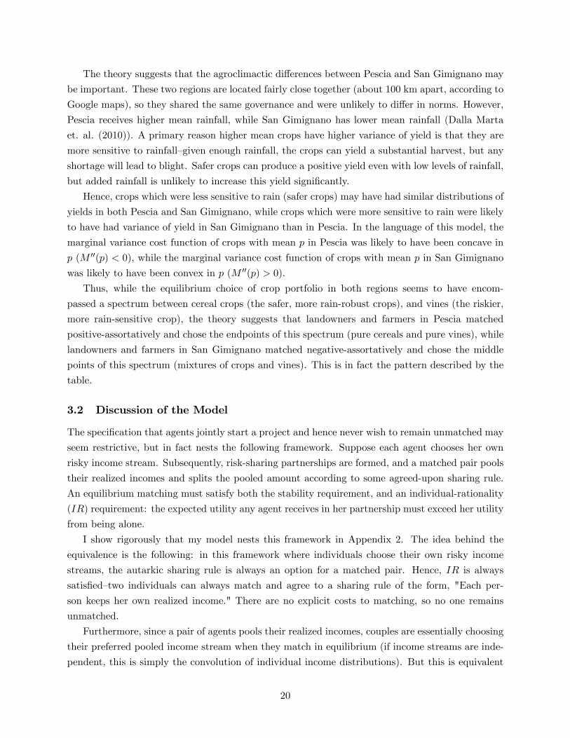
The theory suggests that the agroclimactic di¤erences between Pescia and San Gimignano may

be important. These two regions are located fairly close together (about 100 km apart, according to

Google maps), so they shared the same governance and were unlikely to di¤er in norms. However,

Pescia receives higher mean rainfall, while San Gimignano has lower mean rainfall (Dalla Marta

et. al. (2010)). A primary reason higher mean crops have higher variance of yield is that they are

more sensitive to rainfall�given enough rainfall, the crops can yield a substantial harvest, but any

shortage will lead to blight. Safer crops can produce a positive yield even with low levels of rainfall,

but added rainfall is unlikely to increase this yield signi�cantly.

Hence, crops which were less sensitive to rain (safer crops) may have had similar distributions of

yields in both Pescia and San Gimignano, while crops which were more sensitive to rain were likely

to have had variance of yield in San Gimignano than in Pescia. In the language of this model, the

marginal variance cost function of crops with mean p in Pescia was likely to have been concave in

p (M 00(p) < 0), while the marginal variance cost function of crops with mean p in San Gimignano

was likely to have been convex in p (M 00(p) > 0).

Thus, while the equilibrium choice of crop portfolio in both regions seems to have encom-

passed a spectrum between cereal crops (the safer, more rain-robust crops), and vines (the riskier,

more rain-sensitive crop), the theory suggests that landowners and farmers in Pescia matched

positive-assortatively and chose the endpoints of this spectrum (pure cereals and pure vines), while

landowners and farmers in San Gimignano matched negative-assortatively and chose the middle

points of this spectrum (mixtures of crops and vines). This is in fact the pattern described by the

table.

3.2 Discussion of the Model

The speci�cation that agents jointly start a project and hence never wish to remain unmatched may

seem restrictive, but in fact nests the following framework. Suppose each agent chooses her own

risky income stream. Subsequently, risk-sharing partnerships are formed, and a matched pair pools

their realized incomes and splits the pooled amount according to some agreed-upon sharing rule.

An equilibrium matching must satisfy both the stability requirement, and an individual-rationality

(IR) requirement: the expected utility any agent receives in her partnership must exceed her utility

from being alone.

I show rigorously that my model nests this framework in Appendix 2. The idea behind the

equivalence is the following: in this framework where individuals choose their own risky income

streams, the autarkic sharing rule is always an option for a matched pair. Hence, IR is always

satis�ed�two individuals can always match and agree to a sharing rule of the form, "Each per-

son keeps her own realized income." There are no explicit costs to matching, so no one remains

unmatched.

Furthermore, since a pair of agents pools their realized incomes, couples are essentially choosing

their preferred pooled income stream when they match in equilibrium (if income streams are inde-

pendent, this is simply the convolution of individual income distributions). But this is equivalent

20

to couples explicitly jointly choosing a risky project from some spectrum, and assuming that no

agent stays unmatched. This latter speci�cation is much more natural for an analysis of income-

smoothing, consumption-smoothing, and endogenous matching.

In this model, I also assume that returns are normally-distributed. The normal distribution

has a "representational convenience", in that it has the feature that the only nonzero cumulants19

are the mean and the variance. A natural concern is that this "representational convenience" is

driving the result.

I solve a generalization of the model under the assumption that returns follow an arbitrary

symmetric distribution, and show that normality is not driving the result. The normal distribution

does generate unusual tractability: the mean-variance characterization yields a natural parameter-

ization of the risky project space, so that the function V (p) captures entirely the "cost" of gains in

expected return in terms of variance, since there are no higher order cumulants. But consideration

of a generalized model shows that the key underlying determinant of equilibrium matching is still

a cost-bene�t tradeo¤ across the spectrum of risky projects, where this tradeo¤ is simply less con-

cise than it was before: the "cost" of gains in expected return is now captured by the sum of all

the higher order cumulants, not just the variance. But the sum of all the higher-order cumulants

essentially acts as a "generalized variance" in this context�the su¢ cient condition for matching is

still a parametric condition which can be calculated. Thus, there is no loss in economic insight by

speci�cally assuming normally-distributed returns. Please refer to Appendix 1 for more details and

results for the generalized model.

A third piece of the model is the restriction to groups of size two. Costly state veri�cation does

provide a logical upper bound on group size. However, this assumption plays a key role in the

theory. It is indeed a restriction, but there is a very sharp modeling tradeo¤ between richness of

action space and richness of link formation. Focusing on a network of pairs allows me to optimize

over the whole space of sharing rules and projects, so I can analyze how the tradeo¤between income-

smoothing and consumption-smoothing within a pair in�uences the composition of the equilibrium

network. This would not be possible if I allowed for any kind of match formation.

A �nal piece of the model is the two-sidedness of the matching problem. Why not one-

sided matching? The primary reason for this is technical: under one-sided matching, "negative-

assortative" and "positive-assortative" no longer uniquely identify matching patterns. That is,

when there are two distinct groups of agents, e.g. G1 = f1; 2; 3g and G2 = f3; 4; 5g, the positive-assortative matching is clearly (1; 3); (2; 4); (3; 5). However, if there were only one group of agents,

G = f1; 2; 3; 3; 4; 5g, then (1; 3); (2; 3); (4; 5) is also a positive-assortative matching pattern. More-over, theoretically there may be problems with existence in one-sided matching problems. These

reasons are clearly super�cial�it is clear that the assumption of two-sided matching is merely for

convenience, and does not detract from any deeper economic insight.

19Recall that the cumulant-generating function is the log of the moment-generating function. The �rst and secondcumulants of any distribution are the mean and the variance.

21

4 Policy

In this section, I show how to use the theory to analyze the aggregate and distributional welfare

imapcts of a hypothetical policy. The natural social welfare function in this setting is the total sum

of certainty-equivalents (see the discussion at the end of the Results section).

Using the theory concretely requires consideration of a few practical issues. For example, the

practical issue of the potential for the two groups in a population to be of di¤erent sizes (e.g. there

may be more tenant farmers than landowners) is addressed in the following subsection.

4.1 Di¤erently-sized groups

The assumption of equally-sized groups is unlikely to hold in real-world settings. In the benchmark

model, it is a convenient and relatively harmless assumption to make, because the focus of the

theory is on the relationship between the scope of income-smoothing and consumption-smoothing

informal insurance strategies in a partnership, and the risk composition of equilibrium partnerships,

and this insight does not depend on group size.

However, if we want to use this framework to evaluate policies, we need to account for the

possibility of di¤erently-sized groups, because this could conceivably a¤ect, among other things,

the magnitude of the policy impact. To consider an extreme example, if one group consists only of

one person, while the other group consists of some large number of people, then the individual in

the �rst group may change partners in response to the policy, but most people will be una¤ected.

Therefore, to realistically think about policy, we need to understand what would happen in this

model if the two groups were of di¤erent sizes.

Lemma 7 If jG1j < jG2j (jG1j > jG2j) the most risk-averse excess agents of G2 (G1) will beunmatched. The remaining agents are matched according to the main result (Proposition 2).

A proof is provided in Appendix 7.

Hence, we see that if there are more tenant farmers than landlords, for example, the most

risk-averse tenant farmers will be unmatched, and we can use the conditions from Proposition 2 to

think about the endogenous matching between the remaining farmers and landlords.

4.2 Crop price stabilization/Introduction of formal insurance

Price stabilization, particularly of crops, is frequently proposed by governments as a tool for al-

leviating the substantial risk burden shouldered by the poor (Knudsen and Nash (1990), Minot

(2010)). Farmers face a large amount of yield and price risk. Crop price stabilization should there-

fore reduce the income risk of farmers, and should particularly bene�t the most risk-averse, poorest

agents (Dawe (2001)).

A key contribution of my framework is to illuminate the importance of accounting for the

endogenous informal risk-sharing network response when analyzing the costs and bene�ts of such

a policy, a point that, to my knowledge, has not yet been made in the literature.

22

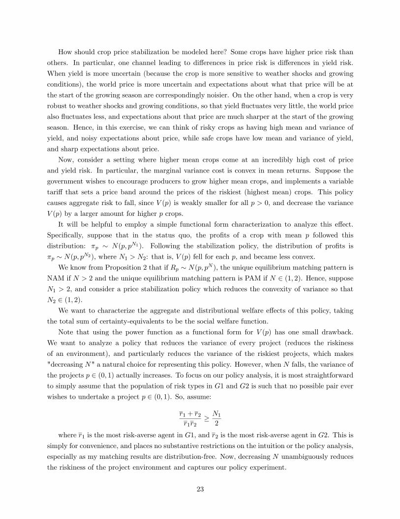
How should crop price stabilization be modeled here? Some crops have higher price risk than

others. In particular, one channel leading to di¤erences in price risk is di¤erences in yield risk.

When yield is more uncertain (because the crop is more sensitive to weather shocks and growing

conditions), the world price is more uncertain and expectations about what that price will be at

the start of the growing season are correspondingly noisier. On the other hand, when a crop is very

robust to weather shocks and growing conditions, so that yield �uctuates very little, the world price

also �uctuates less, and expectations about that price are much sharper at the start of the growing

season. Hence, in this exercise, we can think of risky crops as having high mean and variance of

yield, and noisy expectations about price, while safe crops have low mean and variance of yield,

and sharp expectations about price.

Now, consider a setting where higher mean crops come at an incredibly high cost of price

and yield risk. In particular, the marginal variance cost is convex in mean returns. Suppose the

government wishes to encourage producers to grow higher mean crops, and implements a variable

tari¤ that sets a price band around the prices of the riskiest (highest mean) crops. This policy

causes aggregate risk to fall, since V (p) is weakly smaller for all p > 0, and decrease the variance

V (p) by a larger amount for higher p crops.

It will be helpful to employ a simple functional form characterization to analyze this e¤ect.

Speci�cally, suppose that in the status quo, the pro�ts of a crop with mean p followed this

distribution: �p � N(p; pN1). Following the stabilization policy, the distribution of pro�ts is

�p � N(p; pN2), where N1 > N2: that is, V (p) fell for each p, and became less convex.We know from Proposition 2 that if Rp � N(p; pN ), the unique equilibrium matching pattern is

NAM if N > 2 and the unique equilibrium matching pattern is PAM if N 2 (1; 2). Hence, supposeN1 > 2, and consider a price stabilization policy which reduces the convexity of variance so that

N2 2 (1; 2).We want to characterize the aggregate and distributional welfare e¤ects of this policy, taking

the total sum of certainty-equivalents to be the social welfare function.

Note that using the power function as a functional form for V (p) has one small drawback.

We want to analyze a policy that reduces the variance of every project (reduces the riskiness

of an environment), and particularly reduces the variance of the riskiest projects, which makes

"decreasing N" a natural choice for representing this policy. However, when N falls, the variance of

the projects p 2 (0; 1) actually increases. To focus on our policy analysis, it is most straightforwardto simply assume that the population of risk types in G1 and G2 is such that no possible pair ever

wishes to undertake a project p 2 (0; 1). So, assume:

r1 + r2r1r2

� N12

where r1 is the most risk-averse agent in G1, and r2 is the most risk-averse agent in G2. This is

simply for convenience, and places no substantive restrictions on the intuition or the policy analysis,

especially as my matching results are distribution-free. Now, decreasing N unambiguously reduces

the riskiness of the project environment and captures our policy experiment.

23

There are two e¤ects of altering the shape of V (p): �rst, there is a pure e¤ect from decreasing

the riskiness of an environment (which causes any matched pair to select a higher p project), and

second, there is the endogenous network response resulting from it, which then further a¤ects

welfare.

We know the expression for a partnership�s sum of certainty-equivalents:

CE(r1; r2) = p�(r1; r2)�1

2

r1r2r1 + r2

V (p�(r1; r2))

= V 0�1�2(r1 + r2)

r1r2

�� 12

r1r2r1 + r2

V

�V 0�1

�2(r1 + r2)

r1r2

��Suppose �rst that the matching pattern (NAM) was held �xed when the riskiness of the envi-

ronment was reduced. What would happen to aggregate CE?

CE(r1; r2) = e1

N�1 log�1N2(r1+r2)r1r2

� �1� 1

N

�d

dN= � 1

N(N � 1) log�1

N

2(r1 + r2)

r1r2

�e

1N�1 log

�1N2(r1+r2)r1r2

�< 0

Hence, it is straightforward to see that, in the absence of an endogenous network response,

decreasing N is strictly welfare-improving, both in the aggregate sense and in the individual

(per pair) sense. In other words, if N1 > 2 fell to N2 2 (1; 2), but the match continued to

be negative-assortative, then all pairs would have higher certainty-equivalents and the sum of

certainty-equivalents would increase.

However, as the main result of this paper shows, unless there are exogenous rigidities in match-

ing, the risk-sharing network will not stay �xed. In this example, if N1 > 2 falls to N2 2 (1; 2), theunique equilibrium matching pattern switches from negative-assortative to positive-assortative.

A numeric example clearly illustrates the mechanism by which this policy could have substantial

adverse e¤ects on welfare, particularly for the most risk-averse agents. For example, suppose

G1 = f1; 2; 3; 4g, and G2 = f2; 4; 6; 8g. I want to focus on the welfare e¤ect of the policy derivingfrom the endogenous change in equilibrium matching, and shut down the e¤ect deriving from a

change in the curvature of V (p). A natural way to do this is to consider a small but discrete change

in N , from a value of N under which NAM is the unique equilibrium, to a value of N under which

PAM is the unique equilibrium.

For example, let N1 = 2:1 and N2 = 1:9. So, the levels of the function change very little, but

the marginal variance cost is convex pre-policy and concave post-policy, which we know will shift

the unique equilibrium match from NAM to the other extreme.

Equilibrium project choice then experiences the following change: the red line is before the

policy, and the blue line is after the policy:

24

1 1.5 2 2.5 3 3.5 40.2

0.4

0.6

0.8

1

1.2

1.4

1.6

1.8Equilibrium Project Choice Pre­ and Post­Policy

mea

n pr

ojec

t ret

urn

PrePost

The sum of certainty-equivalents for matched pairs experiences the following change:

1 1.5 2 2.5 3 3.5 40.1

0.2

0.3

0.4

0.5

0.6

0.7

0.8Equilibrium Pairwise Expected Utility Pre­ and Post­Policy

pairw

ise 

expe

cted

 util

ity

PrePost

Clearly, there is more dispersion and inequality in joint expected utilities post-policy, where the

most risk-averse agents partnered with each other are the worst o¤. However, we might also want

to know what happens to individual utilities. Such analysis is challenging in a model of endogenous

matching, as the vector of equilibrium individual expected utilities is not unique (please refer to the

discussion in the Results section). Rather, there is a degree of freedom, which is the equilibrium

expected utility received by one agent. Once this is speci�ed (for any agent), the equilibrium

expected utilities of each individual in the rest of the population are pinned down.

Because risk reduction policies are generally intended to target the most risk-averse people,

let us study the vector of equilibrium expected utilities where the most risk-averse agent in group

two20 is best o¤�that is, the most risk-averse agent in group two has a higher utility in this vector

than any other possible vector of equilibrium expected utilities.

Comparing pre- and post-policy individual utilities of group one and group two:

20Equivalently, group one.

25

1 1.5 2 2.5 3 3.5 40.35

0.4

0.45

0.5

0.55

0.6

0.65

0.7

0.75

0.8Equilibrium Individual Utility of Agents in Group One

risk aversion

expe

cted

 util

ity

PrePost

1 1.5 2 2.5 3 3.5 4­0.25

­0.2

­0.15

­0.1

­0.05

0Equilibrium Individual Utility of Agents in Group Two

risk aversion

expe

cted

 util

ity

PrePost

We see that the more risk-averse agents in group one and group two are worse o¤ after imple-

mentation of the policy, purely as a result of the endogenous network response: a price stabilization

policy intended to reduce the risk burden of the poor, and particularly the risk of the higher mean

yield crops, may actually decrease aggregate welfare21 and increase the risk borne by the most risk-

averse agents, precisely because the policy causes the least risk-averse agents to abandon their roles

as informal insurers of the most risk-averse, in favor of entrepreneurial partnerships with fellow less

risk-averse agents.

This intuition adds interestingly to a few existing results. Attanasio and Rios-Rull (2000) model

the introduction of formal insurance as a policy which reduces the riskiness of the environment.

They also �nd that such a policy may hurt the welfare of the most risk-averse agents. However,

21As measured by the total sum of certainty-equivalents.

26

their model of (non-endogenous) informal risk-sharing, which builds o¤ Ligon, Thomas, Worrall

(2001), centers around limited commitment�two agents interacting repeatedly can only sustain

informal risk-sharing with the threat of cutting o¤ all future ties for someone who reneges. This

particular type of punishment has the important implication that the value of future ties directly

trades o¤ with equilibrium risk-sharing. So, anything that lowers the cost of autarky (remaining

alone and being informally uninsured) will decrease the level of informal insurance that can be

sustained. They then frame the introduction of formal insurance as a policy that would reduce the

cost of being in autarky, and subsequently argue that the level of informal insurance falls, which

may reduce aggregate welfare.

However, in this paper, commitment is taken to be perfect. Perfect commitment in Attanasio

and Rios-Rull (2000) would preclude the conclusion that the introduction of formal insurance could

hurt the most risk-averse agents, because lowering the cost of autarky matters only through the

punishment of cutting o¤ future ties, which is no longer relevant. I show that, even under perfect

commitment, introducing formal insurance might still reduce the welfare of the most risk-averse

agents, because the composition of the informal risk-sharing network changes in response. In my

model, reducing the riskiness of the environment raises the value of autarky, but it also raises the

value of being in a relationship, and raises it heterogeneously across partnerships of di¤erent risk

compositions.

By contrast, Chiappori et. al. (2011) estimate that the least risk-averse individuals are the ones

left worse o¤ after the introduction of formal insurance. The informal argument is that the least

risk-averse agents are displaced as informal insurers. However, this exactly illuminates the need

for a model of the equilibrium network of relationships�I show that the least risk-averse agents do

leave their roles as informal insurers, but only because they prefer to undertake entrepreneurial

pursuits instead. It would be interesting to see how the estimation changes after accounting for the

endogeneity of matching.

5 Testing the Theory: An Experiment

This model provides a natural setting for an experimental test of the theory. In this section, I

propose a basic experimental design to test the key predictions. First, I discuss subject and setting

choice. Next, I describe important elements of the setup. In particular, I describe how to elicit risk

type, and how to design di¤erent sets of gamble choices. Finally, I outline the empirical strategy

suggested by the main theorem and corollary from Section 4.

5.1 Subject and Setting Choice

The theoretical framework is a good �t for an agricultural context. As discussed in the introduction

and background sections, farmers in a broad cross-section of regions are demonstrably risk-averse,

and heterogeneous in their risk aversion. Moreover, this heterogeneity in risk aversion translates

into a heterogeneity in equilibrium behavior; in particular, crop portfolios, spatial plot cohices,

27

input and irrigation choices, and openness to innovative techniques varies by farm. Finally, there

are plenty of examples of the prevalence of collectivity in farming�farmers seeking advice from each

other, farmers entering risk-sharing agreements and self-help groups with each other, and most

directly, landowners employing farmers, for example as sharecroppers.

This suggests several advantages in selecting subjects from villages which are primarily agri-

cultural, and, correspondingly, recruiting subjects for whom farming is the primary occupation.

This is not because the experimental setup should require subjects to possess farming expertise,

but rather because the strong connection between their lives and the task of choosing amongst

gambles with di¤ering yield distributions gives us a measure of con�dence about the relevance and

intuitiveness of the experiment, and their subsequent comprehension of it.

Since matching pattern regressions will be run at the village level, it will be necessary to have

a reasonably large sample of villages to obtain power. Because the theoretical result is distribution

free, it is able to accommodate heterogeneity in risk type distributions across villages. Villages

should be chosen which do not communicate with each other, to prevent information about the

experiment from spreading. Characteristics of the villages should be recorded, such as geographical

location, agroclimate, size, primary occupation, average income, and proximity to urban center.

Field o¢ cers should hold private interview sessions with randomly-chosen households in each

village to extend an invitation to send a member to participate in the experiment. As in Attanasio

et. al. (2010), this should be done only a few days previous to the experiment, to minimize social

selection. Standard characteristics of each interviewed household, and of each adult member of

that household, should be collected, such as ethnicity and religion, physical characteristics of the

dwelling, occupations, income. If the primary occupation is agricultural, collect data on crops

grown, plot size, plot scattering, irrigation, fertilizer, and total harvest.

Additionally, kinship, friendship, neighbor, trust, and employment network data must be col-

lected from households. For example, each interviewed individual may be asked for the names of

her relatives, her friends, her neighbors, the people she trusts most, and the people for whom she

works/whom she employs/with whom she is business partners.

5.2 Setup

5.2.1 Round 1: Risk Elicitation

The experiment will consist of two rounds. In the �rst round, the "risk type elicitation round",

each subject will meet privately with a �eld researcher, where she will be presented with a set

of gambles varying in riskiness and asked to choose one. (The design of this set of gambles is

discussed in detail in the subsection below, "Round 2: Joint Project Choice".) The gamble choice

will be explained pictorially in a manner that accounts for potential illiteracy and unfamiliarity

with probability, and comprehension will be tested. A selection of a gamble with higher mean and

variance will indicate a lower degree of risk aversion than a selection of a gamble with lower mean

and variance. Additionally, each subject will be asked to report what gamble they think the people

they reported trusting the most during the initial household interview would have chosen. This

28

allows us to get a sense of how accurately individuals perceive the risk aversion of those with whom

they are close.

After all risk types have been elicited22, subjects will be gathered in the same room, where

each individual�s gamble choice will be posted publically, again in a manner that accommodates

illiteracy. (Subjects are not told initially that their �rst round gamble choices will be announced.)

The purpose of this announcement is to ensure common knowledge of everyone�s risk types.

5.2.2 Between Rounds: Matching

Following the elicitation of risk types and the public posting of the gamble choices, subjects shall

be randomly divided into two equally-sized groups (if there is an odd number of people, then one

person shall remain unmatched). A researcher will then explain that they will be allowed to pair

up across groups, and that once paired, each pair will be o¤ered the same set of gambles that they

faced in their private �rst rounds, where they will be allowed to choose a project jointly and commit

ex ante to a return-contingent sharing rule of the realized income by reporting their agreed-upon

rule to a researcher, who will enforce it. (Arguments can be made for or against the possible

dependence of the second round gamble choice on �rst round gamble outcomes if the set of gambles

is the same in both rounds, and as Attanasio et. al. (2010) have set a precedent of reusing the �rst

round set, I leave discussion of this question to another forum).

After this explanation of the proceedings of the rest of the game, the subjects will be given half

an hour to establish partnerships (if an individual chooses to remain unmatched, she will receive 0

for sure because she will not be allowed to select a gamble. Since the supports of all gambles are

positive, nobody should choose to remain unmatched as long as there are partners available).

5.2.3 Round 2: Joint Project Choice

Once partnerships have been established, researchers will visit each pair privately to take down

their joint project choice and the sharing rule they have agreed upon. Then, researchers will draw

a realization from each pair�s project choice, and distribute funds according to the sharing rules

that were reported to them. This will mark the end of the experiment.

The key to the experimental test of the theory is the design of the set of gambles from which

matched pairs are asked to choose. Recall that the conditions for unique positive-assortative and

negative-assortative matching emerging from the model in Section 4 centered on the rate of cur-

vature of the mean-variance tradeo¤ across the spectrum of available projects. In the model, the

tradeo¤ between the desire to match with someone with a di¤erent risk type in order to smooth

a given risk in a mutually satisfying way, and the desire to match with someone with a similar

risk type in order to choose a mutually agreeable risk, is captured by this rate of curvature of the

22The Rabin (2000) critique does apply here, but many experiments elicit risk in the literature in this way, so byrevealed preference the payo¤ in economic insight seems to be worth it. Moreover, in this paper, if the environment issuch that the marginal variance cost function is globally convex or concave, then all we need from the risk elicitationround is the ordinal risk attitudes.

29

mean-variance tradeo¤. When a slightly higher mean return corresponds with a drastically higher

variance of return, so that the di¤erence in variance of a low mean return project and a high mean

return project is extremely stark, negative-assortative matching is more likely to result, since all

possible pairs prefer the safer, low mean return project. On the other hand, when a small in-

crease in mean return corresponds to a moderately higher increase in variance, positive-assortative

matching is more likely to result, since there is signi�cant disagreement about preferred project:

less risk-averse people prefer riskier projects, while more risk-averse people prefer safer projects.

Hence, the theory suggests a clear intuition for designing sets of gamble choices: within a

given set, gambles should di¤er in mean and variance of return, with higher mean gambles having

correspondingly higher variances, and the shape of this mean-variance tradeo¤ should di¤er across

di¤erent sets of gamble choices.

For example, a reasonable approach would be to design two types of gamble sets, each containing

�ve gambles. Villages in the sample would be randomly allocated into two groups, where villages in

the �rst group face the �rst set of gamble choices, and villages in the second group face the second

set of gamble choices. Indexing set by superscript i, and gamble by subscript j, the challenge

is to choose values for (pij ; Vij ), the mean and variance of gamble j in set i, for i 2 f1; 2g and

j 2 f1; 2; 3; 4; 5g.There are three signi�cant feasibility constraints imposed by the realism of an experiment that

prevent us from directly applying the theoretical result to this design problem.

1. The return distributions of the gambles must have positive, bounded supports. It seems unwise

to extract money from an experimental subject by declaring that she received a "negative

realization", and it seems expensive to allow for the possibility of a realization of in�nity.

The relevant implication is that we cannot o¤er gambles with distributions that are literally

distributed normally.

2. The set of gamble choices is discrete. The key idea in the theoretical model was not that a

continuum of projects existed literally, but rather that activity diversi�cation (e.g. intercrop-

ping) enabled a spectrum of mean returns with corresponding variances that were higher for

higher means (an upper envelope).

In the experiment, subjects are not allowed to create portfolios of projects; instead, they must

select a single gamble. This can be thought of as re�ecting rigidities in activity diversi�cation

(e.g. intercropping is not possible because of soil type), and limits a pair�s ex ante risk

management ability. An individual r�s desire to pair up with another individual r because

they share project preferences is dampened by the fact that �rst, their favorite project is

unlikely to be available in the small set of gamble choices, and second, because there is not a

wide range of choices, individuals of other risk types will cluster with r on project choice.

The relevant implication of this is that distinct pairs are no longer guaranteed to select distinct

projects. Instead, there will be "clustering" on each of the gamble choices; the degree of this

30

"clustering" depends on the distribution of risk types in the population and on the shape of

the mean-variance tradeo¤.

3. Limited liability holds in an experimental setting. In the theory, the return-contingent sharing

rule of a pair is completely unconstrained. In the experiment, this will not be the case. If for

example a gamble�s realized return is 0, then each partner must receive 0.

This constraint is the most serious, because it inhibits the transferability of expected utility.

For example, if 0 is in the support of a gamble�s return distribution, then partners cannot

agree to nonzero state-independent transfers. This restriction on the sharing rule limits the

pair�s ex post risk management ability, and, importantly, limits di¤erent pairs di¤erently

depending on risk type composition. A quite risk-averse individual r�s desire to pair up with

a much less risk-averse individual r0 << r is dampened by the fact that, because of limited

liability, r0 may not be able to ensure her a return-independent transfer.

Hence, the pairwise sum of certainty-equivalents calculated in Section 2 holds only a bounded

range of divisions v of the expected utility pie, where these bounds depend on risk type and

therefore in�uence endogenous partner choice.

Because of these three limitations of the experimental environment, it is necessary to construct

an "experimental model" satisfying these constraints which captures the essence of the theory:

given a population of heterogeneously risk-averse agents, the risk relationship of the gambles to

each other in the available choice set determines whether positive-assortative or negative-assortative

matching results.

The idea is the following. Recall that the sum of N > 2 independent draws from a uni[a; b]

distribution approximates a normal distribution on the support [Na;Nb]. For example, if a = 0

and b = 1, the convolution of the N densities is (�gure taken from Grimstead and Snell, Chapter

7, Intro to Probability 1997):

This allows us to o¤er gambles whose returns are approximately normally-distributed on bounded,

positive supports. This ensures feasibility of experimental payments and allows us to apply our un-

derstanding of the role played by the mean-variance tradeo¤ from the theoretical results of Section

3.

Therefore, experimental subjects should be asked to choose from one of the following �ve gam-

bles:

1. Receive the sum of N independent draws from a distribution which yields x for sure. (This

is the safe choice.)

2. Receive the sum of N independent draws from a uni[a2; b2] distribution, where:

a2 < x < b2a2 + b22

> x

31

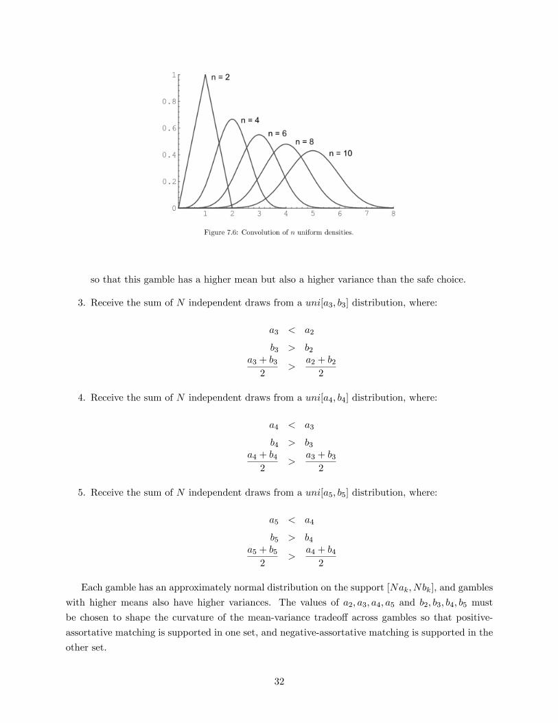
so that this gamble has a higher mean but also a higher variance than the safe choice.

3. Receive the sum of N independent draws from a uni[a3; b3] distribution, where:

a3 < a2

b3 > b2a3 + b32

>a2 + b22

4. Receive the sum of N independent draws from a uni[a4; b4] distribution, where:

a4 < a3

b4 > b3a4 + b42

>a3 + b32

5. Receive the sum of N independent draws from a uni[a5; b5] distribution, where:

a5 < a4

b5 > b4a5 + b52

>a4 + b42

Each gamble has an approximately normal distribution on the support [Nak; Nbk], and gambles

with higher means also have higher variances. The values of a2; a3; a4; a5 and b2; b3; b4; b5 must

be chosen to shape the curvature of the mean-variance tradeo¤ across gambles so that positive-

assortative matching is supported in one set, and negative-assortative matching is supported in the

other set.

32

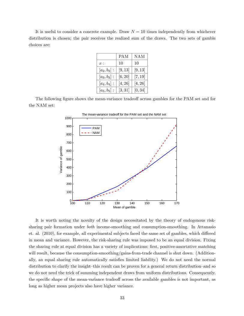
It is useful to consider a concrete example. Draw N = 10 times independently from whichever

distribution is chosen; the pair receives the realized sum of the draws. The two sets of gamble

choices are:

PAM NAM

x : 10 10

[a2; b2] : [9; 13] [9; 13]

[a3; b3] : [6; 20] [7; 19]

[a4; b4] : [4; 26] [4; 26]

[a5; b5] : [3; 31] [0; 34]

The following �gure shows the mean-variance tradeo¤ across gambles for the PAM set and for

the NAM set:

100 110 120 130 140 150 160 1700

100

200

300

400

500

600

700

800

900

1000The mean­variance tradeoff for the PAM set and the NAM set

Mean of gamble

Var

ianc

e of

 gam

ble

PAMNAM

It is worth noting the novelty of the design necessitated by the theory of endogenous risk-

sharing pair formation under both income-smoothing and consumption-smoothing. In Attanasio

et. al. (2010), for example, all experimental subjects faced the same set of gambles, which di¤ered

in mean and variance. However, the risk-sharing rule was imposed to be an equal division. Fixing

the sharing rule at equal division has a variety of implications: �rst, positive-assortative matching

will result, because the consumption-smoothing/gains-from-trade channel is shut down. (Addition-

ally, an equal sharing rule automatically satis�es limited liability.) We do not need the normal

distribution to clarify the insight�this result can be proven for a general return distribution�and so

we do not need the trick of summing independent draws from uniform distributions. Consequently,

the speci�c shape of the mean-variance tradeo¤ across the available gambles is not important, as

long as higher mean projects also have higher variance.

33

Allowing for consumption-smoothing by endogenizing a risk-sharing group�s sharing rule, in

addition to endogenous choice of income stream, entails the precise design of di¤erent sets of gamble

choices. Since the e¤ect of the tradeo¤ between consumption-smoothing and income-smoothing on

equilibrium matching is best distilled with normally-distributed returns, one idea is to replicate

such a distribution in a feasible way by summing N independent draws from uniform distributions,

which di¤er in mean and variance.

5.3 Empirical Strategy

Recall from Proposition 4 that support for the theory in the data would be observation of at least one

of the following: (a) people match positive-assortatively in risk attitudes, and the observed means

of equilibrium risky projects are convex in the representative rates of risk aversion of matched pairs;

(b) people match negative-assortatively in risk attitudes, and the observed means of equilibrium

risky projects are concave in the representative rates of risk aversion of matched pairs.

The basic empirical strategy consists of 3 steps. First, given a dataset containing Z villages,

index a village by k. Then:

1. For each village k, characterize the equilibrium matching pattern (the correlation between

the probability that individual i is matched with individual j and their corresponding risk

types ri and rj). Is the equilibrium matching pattern the "correct" one, that is, the pattern

which was meant to be induced by the set of gamble choices o¤ered to that village?

2. Next, examine the behavior of equilibrium project choices and the risk composition of the

matched pairs.

3. Then, characterize the relationship between the equilibrium matching pattern and the equi-

librium behavior of project choice in risk types across all villages. If we observe convexity of

project choice in the representative rates of risk aversion of matched pairs corresponding with

positive-assortative matching, and/or concavity of project choice in the representative rates

of risk aversion of matched pairs corresponding with negative-assortative matching, then this

is support for the theory.

To be a little more speci�c, �rst focus on data from a given village k. Suppose that village k

was o¤ered the "positive-assortative" set of gamble choices, so we should expect positive-assortative

matching.

To glean the matching pattern from the data, set the observation level to be a dyad (i; j) of an

individual i in group one matched with an individual j in group two (recall that the experiment

participants were randomly divided into two equally-sized groups). If each group has M people in

it, then there should be M(M�1)2 total observations.

De�ne a variable that describes the distance between the risk attitudes of i and j:

�ij = jri � rj j

34

Note that this is symmetric: �ij = �ji.

Now, de�ne a variable mij :

mij =

(1; i matched with j

0; else

So, mij is also symmetric.

Then, for each village k, regress the linkage variable mij on the distance between risk attitudes,

�ij , and the pre-existing networks Xkij (e.g. kinship):

mkij = �

k + �k�kij +Xkij + "

kij

If �k > 0, the matching pattern is closer to being negative-assortative, since large di¤erences in

risk attitudes increase the probability that two individuals are linked, while if �k < 0, the matching

pattern is closer to being positive-assortative, since small di¤erences in risk attitudes increase the

probability that two individuals are linked.

Con�rm that the matching pattern of village k is the pattern that was meant to be induced by

the set of gamble choices o¤ered to village k.

Now, look at matched dyads in village k only, and denote the mean of the equilibrium project

choice of a matched (i; j) by pij .

For each matched dyad (i; j), calculate the representative rate of risk aversion:

~Hij =1

ri+1

rj

For the matched dyads in each village k, regress:

pkij = ck + �krki + �

krkj + k�~Hkij

�2+ V k + �kij

where V k is village �xed e¤ects.

It should be the case that �k; �k < 0 for all k, since more risk-averse individuals should choose

safer (lower mean) gambles. If k > 0, then equilibrium project mean is convex in the rate of risk

aversion, and if k < 0, then equilibrium project mean is concave in the rate of risk aversion.

Finally, regress:

�k = �+ � k + �

to ascertain the relationship in village k between the equilibrium matching pattern and the

behavior of equilibrium projects in risk types.

Support for the model is � > 0: this indicates that convexity of mean income in the represen-

tative rates of risk aversion of a linked pair corresponds with positive-assortative matching, while

concavity of mean income in the representative rates of risk aversion of a linked pair corresponds

with negative-assortative matching.

35

6 Conclusion

This paper proposes a novel framework for thinking about endogenous matching between hetero-

geneous agents as resulting from the tradeo¤ of two general forces: one, a "gains from trade"

force, which favors matching between unlike types, and the other, a "similarity of perspective"

force, which favors matching between like types. Speci�cally, conditional on facing a given risk,

a less risk-averse agent and a more risk-averse agent bene�t from being matched with each other,

because the less risk-averse agent is willing to sell insurance which the more risk-averse agent is

willing to buy. But conditional on being able to choose what risk to face, agents prefer partners

with similar risk attitudes. In other words, consumption-smoothing forces push the match to be

negative-assortative, while income-smoothing forces push the match to be positive-assortative.

I show that the equilibrium composition of risk-sharing pairs depends critically on the interaction

between consumption-smoothing and income-smoothing as risk management tools, and in particular

the di¤erential evaulation of this interaction across agents of di¤erent risk attitudes. I show that this

interaction is cleanly captured by the convexity of the marginal variance cost function in expected

returns of projects, and provide testable conditions that tie the theory to data. In particular,

I describe observable di¤erences in the environments in which each type of assortative matching

pattern emerges, and use these di¤erences to construct a testable falsi�ability condition based on

the relationship of the mean returns of equilibrium projects to the risk composition of matched

pairs. I �nd preliminary support for the theory in existing literature.

But why should we care about understanding these matching forces? This theory has a variety of

meaningful implications for policy. For example, even under perfect commitment in the contracting

environment, a risk-reduction policy which reduces the risk of higher mean, higher variance projects

in particular, may decrease aggregate welfare and leave the most risk-averse agents strictly worse

o¤, purely because of the endogenous network response: the least risk-averse agents abandon their

roles as "informal insurers" of the most risk-averse, preferring entrepreneurial partnerships with

fellow less risk-averse agents instead.

Accounting for endogeneity would also a¤ect the analysis of a variety of land reform policies

discussed in the literature. For example, Banerjee (2000) points out that the e¤ects of land redistri-

bution cannot be estimated without understanding the reasons behind the status quo distribution

of land in the �rst place. If the distribution of land served a risk-sharing purpose, or alterna-

tively, if agents optimized their risk-sharing activities given the land distribution (for example,

large landowners provide informal insurance to the landless), then land redistribution may either

have no e¤ect, as people implicitly ignore it, or may actually hurt informal insurance.

Improving the security of tenant farmers is another common land reform. For example, Banerjee

et. al. (2002) discuss Operation Barga, a 1970s West Bengali land reform which diminished the

ability of landlords to expel their tenants. An unexplored e¤ect of such a reform is the added

matching friction: relationships will be unable to respond optimally to changes in the environment.

For example, if a bad rainfall shock unexpectedly hits a farming village, increasing the steepness of

the mean-variance tradeo¤ across crop choices, it would be e¢ cient for less risk-averse individuals

36

to embrace their role as informal insurers and provide insurance to more risk-averse individuals on

safer crops. If Barga had locked less risk-averse individuals in their relationships with other less

risk-averse individuals before the shock, they will not be able to adjust towards e¢ ciency. On the

other hand, if Barga had locked the less risk-averse into relationships with the more risk-averse, and

then the government began subsidizing innovations (reducing the variance of high mean projects),

the less risk-averse individuals would like to switch to less risk-averse partners and take up these

innovations, but will be legally prevented from doing so.

Finally, accounting for endogeneity may substantially alter our inferences from empirical ob-

servations. For example, an observation that the strength of dependence of a sharecropper�s rent

contract on realized harvest is positively correlated with the riskiness of the crop grown may tempt

us to conclude that risk is not a problem for farmers, since risk considerations do not appear to

in�uence contract design (Allen and Lueck (1992)). However, if more risk-averse farmers work for

less risk-averse landowners, cultivating safer crops under low-powered contracts, while less risk-

averse farmers work for more risk-averse landowners, cultivating riskier crops under high-powered

contracts, the same empirical observations would emerge, but risk concerns would be playing a sig-

ni�cant role in contract design, through the unaccounted-for channel of contracting partner choice.

All sorts of challenges remain. This model can clearly be enriched in many ways�by generalizing

preferences and the project space, by introducing limited commitment or incomplete information, by

allowing for more complex forms of group formation, or by adding dynamics to study the feedback

between riskiness of project choice and investment capability, to characterize a potential innovation

trap. The main contribution of this paper is to propose a tractable model of the endogenous

formation of risk-sharing relationships, upon which further dimensions can be layered, and to show

that even this simple model can lead to substantial changes in our understanding of numerous policy

debates. The unique environments of developing economies make design problems particularly

challenging, but it is the magnitude of the stakes which makes them particularly important.

7 References

1. Ackerberg, D. and M. Botticini. "Endogenous Matching and the Empirical Determinants of

Contract Form." Journal of Political Economy (110) 2002 564-590.

2. Akanda, M., H. Isoda, and S. Ito. "Problem of Sharecrop Tenancy System in Rice Farming in

Bangladesh: A Case Study on Alinapara Village in Sherpur District." Journal of Int. Farm

Management (4) 2008 23-30.

3. Alderman, H. and C. Paxson. "Do the Poor Insure? A Synthesis of the Literature on Risk

and Consumption in Developing Countries." Economics in a Changing World, vol. 4 1992

49-78.

4. Allen, D. and D. Lueck. "Contract Choice in Modern Agriculture: Cash Rent versus Crop-

share." Journal of Law and Economics (35) 1992 397-426.

37

5. Antle, J. "Econometric Estimation of Producers� Risk Attitudes." Amer. Journal of Ag.

Econ. (69) 1987 509-522.

6. Attanasio, O., A. Barr, J. Cardenas, G. Genicot, and C. Meghir. "Risk Pooling, Risk Prefer-

ences, and Social Networks." Amer. Econ. Journal: Applied Economics (4) 2012 132-167.

7. Attanasio, O. and J. Rios-Rull. "Consumption Smoothing in Island Economies: Can Public

Insurance Reduce Welfare?" European Economic Review (44) 2000 1225-1258.

8. Banerjee, A. "Prospects and Strategies for Land Reforms." Annual World Bank Conference

on Development Economics 1999, eds. B. Pleskovic and J. Stiglitz. 253-284.

9. Banerjee, A., P. Gertler, and M. Ghatak. "Empowerment and E¢ ciency: Tenancy Reform

in West Bengal." Journal of Political Economy (110) 2002 239-280.

10. Bardhan, P. "Interlocking Factor Markets and Agrarian Development: A Review of Issues."

Oxford Econ. Papers (32) 1980 82-98.

11. Basu, K. "Limited Liability and the Existence of Share Tenancy." J. Dev. Econ. (38) 1992

203-220.

12. Becker, G.S. "A Theory of Marriage: Part I." Journal of Political Economy (81) 1973 813-846.

13. Bellemare, M. "Sharecropping, Insecure Land Rights and Land Titling Policies: A Case Study

of Lac Alaotra, Madagascar." Development Policy Review (27) 2009 87-106.

14. Besley, T. "Savings, Credit, and Insurance." Handbook of Development Economics (3) 1995

2123-2207.

15. Binswanger, H.P. "Attitudes towards Risk: Experimental Measurement in Rural India." Am.

J. Agr. Econ. (62) 1980 395-407.

16. Bloch, F. et. al. "Informal Insurance in Social Networks." J. Econ. Theory (14) 2008 36-58.

17. Bold, T. "Implications of Endogenous Group Formation for E¢ cient Risk-Sharing." The

Economic Journal (119) 2009 562-591.

18. Bramoulle, Y. and R. Kranton. "Risk Sharing Networks." J. Econ. Behavior and Organiza-

tion (64) 2007 275-294.

19. Chandrasekhar, A. et. al. "Testing Models of Social Learning on Networks: Evidence from a

Framed Field Experiment." Working Paper 2012.

20. Chiappori, P-A., K. Samphantharak, S. Schulhofer-Wohl, and R. Townsend. "Heterogeneity

and Risk-Sharing in Village Economies." Working Paper 2011.

21. Chiappori, P-A. and P. Reny. "Matching to share Risk." Working Paper 2006.

38

22. Insurance Against Poverty. ed. Stefan Dercon. 2004.

23. Dalla Marta, A., M. Mancini, R. Ferrise, M. Bindi, and S. Orlandini. "Energy crops for

biofuel production: Analysis of the potential in Tuscany." Biomass and Bioenergy (34) 2010

1041-1052.

24. Dawe, D. "How far down the path to free trade? The importance of rice price stabilization

in developing Asia." Food Policy (26) 2001 163-175.

25. Dercon, S. "Risk, Crop Choice, and Savings: Evidence from Tanzania." Econ. Dev. and

Cultural Change (44) 1996 483-513.

26. Dercon, S. and P. Krishnan. "In Sickness and in Health: Risk Sharing within Households in

Rural Ethiopia." Journal of Political Economy (108) 2000 688-727.

27. Fafchamps, M. "Risk-sharing Between Households." Handbook of Social Economics 2008.

28. Fafchamps, M. and A. Lund. "Risk-sharing Networks in Rural Phillippines." J. Dev. Econ.

(71) 2003 261-287.

29. Fafchamps and Gubert. "The Formation of Risk-Sharing Networks." J. Dev. Econ. (83) 2007

326-350.

30. Genicot, G. and D. Ray. "Group Formation in Risk-Sharing Arrangements." Rev. Econ.

Stud (70) 2003 87-113.

31. Knudsen, O. and J. Nash. "Domestic Price Stabilization Schemes in Developing Countries."

Economic Development and Cultural Change (38) 1990 539-558.

32. Kocherlakota, N. "Implications of E¢ cient Risk-Sharing Without Commitment." Review of

Economic Studies (63) 1996 596-609.

33. Kurosaki, T. "Risk-Sharing Arrangements and the Structure of Risk and Time Preferences:

Theory and Evidence from Village India." Working Paper 1999.

34. Legros, P. and A. Newman. "Beauty is a Beast, Frog is a Prince: Assortative Matching with

Nontrasferabilities (75) 2007 1073-1102.

35. Ligon, E., J. Thomas, and T. Worrall. "Informal Insurance Arrangements with Limited

Commitment: Theory and Evidence from Village Economies." Review of Economic Studies

(69) 2002 209-244.

36. Minot, N. "Food Price Stabilization: Lessons for Eastern and Southern Africa." Risk Man-

agement in African Agriculture Seminar Presentation 2010.

37. Morduch, J. "Income Smoothing and Consumption Smoothing." J. Econ. Perspectives (9)

1995 103-114.

39

38. Rabin, M. "Risk aversion and expected utility theory: A calibration theorem." Econometrica

(68) 2000 1281�1292.

39. Rathore, V.S., J.P. Singh, and R.K. Beniwal. "Rainfed Farming Systems of Hyper Arid

Northwestern Rajasthan: an Analysis." Annals of the Arid Zone (48) 2009 125-131.

40. Rosenzweig, M. "Risk, Implicit Contracts, and the Family in Rural Areas of Low-Income

Countries." Economic Journal (98) 1988 1148-1170.

41. Rosenzweig, M. and H.P. Binswanger. "Wealth, Weather Risk, and the Composition and

Pro�tability of Agricultural Investments." The Economic Journal (103) 1993 56-78.

42. Rosenzweig, M. and O. Stark. "Consumption Smoothing, Migration, and Marriage: Evidence

from Rural India." J. Polit. Econ. (97) 1989 905-926.

43. Schulhofer-Wohl, S. "Negative-assortative Matching of Risk-Averse Agents with Transferable

Expected Utility." Econ. Letters (92) 2006 383-388.

44. Shapley, L. and M. Shubik. "The assignment game I: The Core." Intl. J. Game Theory (1)

1971 111-130.

45. Sharpe, William F. "The Sharpe Ratio". The Journal of Portfolio Management (21) 1994

49�58.

46. Singh, H., G. Singh, J. Samuel, and R. Pathak. "Precision Farming in Horticulture." Pro-

ceedings of the National Seminar Workshop on Hi-Tech Horticulture and Precision Farming,

2003.

47. Stiglitz 1974. "Incentives and Risk Sharing in Sharecropping." Review of Economic Studies

(41) 1974 219-255.

48. Townsend, R. "Optimal Contracts and Competitive Markets with Costly State Veri�cation."

Journal of Economic Theory (21) 1979 265-293.

49. Townsend, R. "Risk and Insurance in Village India." Econometrica (62) 1994 539-591.

50. Townsend, R. and R. Mueller. "Mechanism Design and Village Economies: From Credit to

Tenancy to Cropping Groups." Review of Economic Dyanmics (1) 1998 119-172.

51. Wright, B. "Storage and Price Stabilization." Handbook of Ag. Econ. (1) 2001 818-861.

40

8 Appendices

8.1 A1: The Model with General Distribution of Returns

Suppose all elements of the environment are the same, except now project p has returns distributed

Rp � f(Rpjp), (Rp)?p, for some well-de�ned pdf f(Rpjp) whose moments exist.Given a matched pair (r1; r2), agent r1 solves:

maxs(Rp)

Z 1

�1�e�r1[Rp�s(Rp)]f(Rpjp)dRp s:t:

Z 1

�1�e�r2s(Rp)f(Rpjp)dRp � �e�v

Then the optimal sharing rule is

s�(Rp) =r1

r1 + r2Rp +

1

r2log

Z 1

�1e� r1r2r1+r2

Rpf(Rpjp)dRp +v

r2

where the optimal project solves:

maxp�e

r1r2v�Z 1

�1e� r1r2r1+r2

Rpf(Rpjp)dRp�1+ r1

r2

Then the sum of certainty-equivalents of the pair is:

CE(r1; r2) = ��1

r1+1

r2

�log

Z 1

�1e� r1r2r1+r2

Rpf(Rpjp�(r1; r2))dRp

Denote the harmonic mean of (r1; r2) by H, and one-half the harmonic mean by:

H(r1; r2) =r1r2r1 + r2

We know that a su¢ cient condition for the unique equilibrium matching pattern to be PAM isdCE(r1;r2)dr1dr2

> 0, while we know that dCE(r1;r2)dr1dr2< 0 is su¢ cient for NAM to be the unique equilibrium

matching pattern. What conditions are needed for these two inequalities to hold?

Recognize that the sum of certainty-equivalents is actually just:

CE(r1; r2) = � 1

H(r1; r2)CRp(t = �H(r1; r2))

= �H(r1; r2)p+1Xn=1

H(r1; r2)2n

(2n)!k2n(p)

where CRp(t) is the cumulant-generating function of the random variableRp (where the cumulant-

generating function is log of the moment-generating function).

Impose a symmetric distribution, since we know that all higher-order odd cumulants are zero.

41

Then it is clear that a given risk-averse agent r evaluates a project p by looking at its expected

return and the sum of all its higher order cumulants. Speci�cally, the agent likes expected return,

but expected return comes at a cost, which is a larger sum of higher order cumulants. This can

be thought of as a "cost function" of projects, and can be thought of as sort of a "generalized

variance".

The �rst-order condition characterizing optimal project choice is given by:

FOCp :

1Xn=1

H(r1; r2)2n

(2n)!k02n(p) = H(r1; r2)

while we need the following condition for convexity:

SOCp :

1Xn=1

H(r1; r2)2n

(2n)!k002n(p) � 0

Then di¤erentiate the �rst-order condition implicitly with respect to H:

dp

dH=1�

P1n=1

H(r1;r2)2n�1

(2n�1)! k02n(p)P1n=1

H(r1;r2)2n

(2n)! k002n(p)

But the FOC tells us:

1Xn=1

H(r1; r2)2n

(2n)!k02n(p) = H(r1; r2))

1Xn=1

H(r1; r2)2n�1

(2n)!k02n(p) = 1

and

1Xn=1

H(r1; r2)2n�1

(2n� 1)! k02n(p) >1Xn=1

H(r1; r2)2n�1

(2n)!k02n(p) = 1

So:

dp

dH< 0)

dp

dr1=

dp

dH

dH

dr1< 0

dp

dr2=

dp

dH

dH

dr2< 0

where p�(r1; r2) symmetric in r1; r2 since H(r1; r2) symmetric in r1; r2.

42

8.2 A2: Equivalence of model to alternative with individual project choice,pooled income, and IR

Suppose that a spectrum of projects p � 0 is available, where Rp � N(p; V (p)), where V (p) > 0,V 0(p) > 0, and V 00(p) > 0. Each agent r in G1 and G2 chooses a project pr, and a matched

pair pools their realized incomes and splits it according to a pre-decided pooled-return-contingent

sharing rule, s(Rpr1 +Rpr2 ).

Assume that the income realizations of r1 and r2 are independent (the return of project pr1 is

independent of the return of project pr2). Then the distribution of the pooled income stream is

simply f(Rpjpr1) � f(Rpjpr2) the convolution, with mean pr1 + pr2 and variance V (pr1) + V (pr2).(Actually, since I�ve imposed normal form, Rpr1 + Rpr2 � N(pr1 + pr2 ; V (pr1) + V (pr2)).) Note

that IR is clearly satis�ed, because the autarkic sharing rule (where each person keeps her realized

income) is always an option for the pair, but isn�t chosen in equilibrium.

But note that N(pr1 + pr2 ; V (pr1) + V (pr2)) for pr1 ; pr2 > 0: pr1 = 1; pr2 = 3, then N(4; V (1) +

V (3)), versus pr1 = 2; pr2 = 2, then N(4; V (2) + V (2)) since V () convex, this means that any pair

(r1; r2) would always choose 2; 2 instead of 1; 3=3; 1. Suppose pr1+pr2 = pr1+ pr2 . then because V ()

convex, the lower number is the one with smaller jpr1 � pr2 j (e.g. if the sum is X, then the "best"

sum of projects is X2 ;X2 ). We can partition all possible pairs (pr1 ; pr2) into equivalence classes by

their sum�e.g. the class 4 is represented by the line x + y = 4. Then, call the variance of the

project with mean 4 (class 4), V (2) + V (2). In fact, for class X (which is the mean of the pooled

return), let the variance of this be 2 � V (X2 ) (this is the smallest variance of the pooled return forall pairs of projects having the same expected pooled return). (We do this because we know that

any risk-averse agent deciding between two projects with normally-distributed returns having the

same mean would always choose the one with lower variance.)

This implies that we can think of this problem in the following way: a matched pair jointly

selects a project X with return distributed N(X; 2�V (X2 )), where we can de�ne eV (X) = 2�V (X2 ),a convex function since V () is convex. And, assume IR is satis�ed, that is, that agents would

rather match with any partner and start a project than being alone and not undertaking a project.

But this is the environment I study.

8.3 A3: Proof that NTU problem has TU representation in expected utility

We know from the appendix discussing the generalized model that the indirect utility of an agent

r1 who ensures his partner, r2, a level of expected utility �e�v is:

�(r1; r2; v) = �er1r2v�Z 1

�1e� r1r2r1+r2

Rpf(Rpjp)dRp�1+ r1

r2

Partner r2 of course receives:

EUr2(v) = �e�r2 v

r2

43

Then the certainty-equivalent of each member is:

CEr1(v) = ��1

r1+1

r2

�log

�Z 1

�1e� r1r2r1+r2

Rpf(Rpjp�(r1; r2))dRp�� v

r2

CEr2(v) =v

r2

There is clearly a one-to-one tradeo¤ between the certainty-equivalent of r1 and the certainty-

equivalent of r2. In other words, the slope of the Pareto frontier of expected utility is �1. Hence,expected utility is transferable.

It is also interesting to see that the generalized increasing/decreasing di¤erences technique from

Legros and Newman (2007) corresponds to the supermodularity and submodularity of CE(r1; r2).

Recall the Legros-Newman generalized di¤erences condition for matching under nontransferable

utility: the following is a su¢ cient condition for positive-assortative matching to be the unique

equilibrium matching pattern:

�(r1; r2; p�(r1; r2); v) = �(r1; r

02; p

�(r1; r02); u))

�(r01; r2; p�(r01; r2); v) < �(r01; r

02; p

�(r01; r02); u) 8r1; r2

We want to show that this is equivalent to a transferable utility approach, that is, showing thatdCE(r1;r2)dr1dr2

> 0, where CE(r1; r2) is the sum of certainty-equivalents in a matched pair (r1; r2) (see

previous appendix section).

We know from the proof of the optimal sharing rule and sum of certainty-equivalents in the

general case that the indirect utility of agent r1 when matched with agent r2 and ensuring him

expected utility �e�v is:

�(r1; r2; p�(r1; r2); v) = �e

r1r2v�Z

e� r1r2r1+r2

Rpf(Rpjp�(r1; r2))dRp�1+ r1

r2

So

�(r1; r2; p�(r1; r2); v) = �(r1; r

02; p

�(r1; r02); u),

�er1r2v�Z

e� r1r2r1+r2

Rpf(Rpjp�(r1; r2))dRp�1+ r1

r2

= �er1r02u

"Ze� r1r

02

r1+r02Rpf(Rpjp�(r1; r02))dRp

#1+ r1r02,

r1r2v +

�1 +

r1r2

�log

Ze� r1r2r1+r2

Rpf(Rpjp�(r1; r2))dRp =

r1r02u+

�1 +

r1r02

�log

Ze� r1r

02

r1+r02Rpf(Rpjp�(r1; r02))dRp ,

44

1

r02u� 1

r2v =

�1

r1+1

r2

�log

Ze� r1r2r1+r2

Rpf(Rpjp�(r1; r2))dRp ��1

r1+1

r02

�log

Ze� r1r

02

r1+r02Rpf(Rpjp�(r1; r02))dRp

Then the condition �(r01; r2; p�(r01; r2); v) < �(r

01; r

02; p

�(r01; r02); u) is equivalent to:�

1

r1+1

r2

�log

Ze� r1r2r1+r2

Rpf(Rpjp�(r1; r2))dRp�

�1

r1+1

r02

�log

Ze� r1r

02

r1+r02Rpf(Rpjp�(r1; r02))dRp >

>

�1

r01+1

r2

�log

Ze� r01r2r01+r2

Rpf(Rpjp�(r01; r2))dRp�

�1

r01+1

r02

�log

Ze� r01r

02

r01+r02Rpf(Rpjp�(r01; r02))dRp

That is, the condition is equivalent to the following expression having increasing di¤erences in

(r1; r2):

��1

r1+1

r2

�log

Ze� r1r2r1+r2

Rpf(Rpjp�(r1; r2))dRp

Now, let�s �nd the certainty-equivalent of r1 when she is paired with r2 and ensuring him �e�v:

�e�r1CEr1 = �(r1; r2; p�(r1; r2); v))

CEr1 = � 1r1log [��(r1; r2; p�(r1; r2); v)]

And the certainty-equivalent of r2 is vr2. Then the sum CE(r1; r2) is:

CE(r1; r2) = � 1r1log [��(r1; r2; p�(r1; r2); v)] +

v

r2

= � 1r1

�r1r2v + (1 +

r1r2) log

Ze� r1r2r1+r2

Rpf(Rpjp�(r1; r2))dRp�+v

r2

= ��1

r1+1

r2

�log

Ze� r1r2r1+r2

Rpf(Rpjp�(r1; r2))dRp

But this is exactly the same condition we got from the generalized di¤erences condition from

Legros-Newman.

The argument is analogous for showing that Legros-Newman generalized decreasing di¤erences

45

condition for negative-assortative matching to be the unique equilibrium matching pattern is equiv-

alent to showing that dCE(r1;r2)dr1dr2< 0.

8.4 A4: Proof of main matching result

The cumulant-generating function for a normal distribution N(p; V (p)) has a very nice form:

CRp(t = � bHjp) = � bHp+ bH2

2V (p)

Hence:

CE( bH) = p� 12bHV (p)

Recall that:

bH =r1r2r1 + r2

Then:

dCE(r1; r2)

dr1r2= � r1r2

(r1 + r2)3V

�V 0�1

�2(r1 + r2)

r1r2

��+

2

r1r2(r1 + r2)V 0�10

�2(r1 + r2)

r1r2

�where the project chosen optimally by a pair (r1; r2) is:

p�(r1; r2) = V0�1�2(r1 + r2)

r1r2

�Therefore, dCE(r1;r2)dr1dr2

> 0 i¤:

2(r1 + r2)2

r21r22

V 0�10�2(r1 + r2)

r1r2

�> V

�V 0�1

�2(r1 + r2)

r1r2

��Then, de�ne:

g(x) =x2

2V 0�10 (x)� V (V 0�1(x))

Finding a su¢ cient condition for PAM is equivalent to �nding conditions on V (�) such thatg(x) > 0 for x > 0.

Assume g(0) = 0, that is, V (0) = 0 and V 0(0) = 0. Then:

g0(x) =x2

2V 0�100(x)

So, g0(x) > 0 if V 0�100(x) > 0, V 000(x) < 0 for x > 0, and g0(x) < 0 if V 0�100(x) < 0, V 000(x) >

0, which proves the result.

On the Corollaries: recall that optimal project choice of (r1; r2) is given by:

46

p�(r1; r2) = V0�1�2(r1 + r2)

r1r2

�The su¢ cient condition for PAM to be the unique equilibrium is V 0�100(p) > 0 (V 000(p) < 0).

It is clear that this implies project choice will be convex in the "aggregated type" of the pair,2(r1+r2)r1r2

, that is, optimal project will vary a lot across di¤erent aggregated types. Similarly, if

V 0�100(p) < 0, so that NAM is the unique equilibrium, it is clear that project choice will be concvae

in the "aggregated type" of the pair, that is, optimal project will not vary much across di¤erent

aggregated types.

How does project choice vary in individual type?

dp

dr1= �V 0�10

�2(r1 + r2)

r1r2

��2

r21

�dp

dr2dr1= V 0�100

�2(r1 + r2)

r1r2

�4

r21r22

Clearly, dpdr2dr1

> 0 i¤ V 0�100(p) > 0, and dpdr2dr1

< 0 i¤ V 0�100(p) < 0.

Now, let�s look more closely at the Sharpe ratio of a project p when V (p) = pN , N > 1:

SR(p) =p

V (p)12

= p1�N2

Then:

dSR(p)

dp=

�1� N

2

�p�

N2

Then

dSR(p)

dp> 0 if N 2 (1; 2)

< 0 if N > 2

But N 2 (1; 2) is precisely the condition for PAM to be the unique matching equilibrium, and

N > 2 is precisely the condition for NAM to be the unique matching equilibrium.

8.5 A5: NAM is the unique equilibrium when income-smoothing is shut down

Suppose that all pairs must undertake the same project, p. For instance, the government mandates

that all farmers must grow rice. This e¤ectively shuts down the income-smoothing channel.

47

Di¤erentiate CE(r1; r2) with respect to r1 and r2 when there is no project choice, so that all

pairs (r1; r2) face the same risky income stream f(Rpjp): the cross-partial dCE(r1;r2)dr1dr2is:

� r1r2(r1 + r2)3

Re� r1r2r1+r2

Rpf(Rpjp)dRpRR2pe

� r1r2r1+r2

Rpf(Rpjp)dRp �hRRpe

� r1r2r1+r2

Rpf(Rpjp)dRpi2

hRe� r1r2r1+r2

Rpf(Rpjp)dRpi2

But we know that:

Ze� r1r2r1+r2

Rpf(Rpjp)dRpZR2pe

� r1r2r1+r2

Rpf(Rpjp)dRp >�Z

Rpe� r1r2r1+r2

Rpf(Rpjp)dRp�2

since we know variance is always positive, thus:

Zf(Rpjp)dRp

ZR2pf(Rpjp)dRp >

�ZRpf(Rpjp)dRp

�2and g(Rp) = e

� r1r2r1+r2

Rp is a convex function.

Therefore

dCE(r1; r2)

dr1dr2< 0

and negative-assortative matching results as the unique equilibrium.

This corresponds with the result from Chiappori and Reny (2006) and Schulhofer-Wohl (2006).

8.6 A6: PAM is the unique matching when consumption-smoothing is shutdown

We know from the main matching result that the optimal sharing rule is linear. Suppose the slope

of the sharing rule s(Rp) = a+ bRp is �xed at b for all possible pairs of risk types. (For example,

the government mandates an equal split of the output, but partners are free to make �xed transfers

to each other.)

This removes consumption-smoothing as an e¤ective risk management tool, leaving only income-

smoothing (project choice). What happens to equilibrium risk-sharing relationships?

A matched pair (r1; r2) chooses the relationship-speci�c transfer a and project p:

maxa;p

E[�e�r1[Rp�a�bRp]jp] s.t.

E[�e�r2[a+bRp]jp] � �e�v

The �xed transfer just serves to satisfy the constraint, since the division of output is �xed at b

48

by the government. Therefore:

a =v

r2+r22b2V (p)� bp

Then, the project chosen is:

maxp�e�r1

hp� v

r2�( r12 (1�b)

2+r22b2)V (p)

i

p�(r1; r2) = V0�1�

2

r1(1� b)2 + r2b2

�Then the sum of certainty-equivalents of a given pair (r1; r2) is:

CE(r1; r2) = V0�1�

2

r1(1� b)2 + r2b2

���r12(1� b)2 + r2

2b2�V

�V 0�1

�2

r1(1� b)2 + r2b2

��And:

dCE

dr1= �(1� b)

2

2V

�V 0�1

�2

r1(1� b)2 + r2b2

��dCE

dr2dr1= V 0�10

�2

r1(1� b)2 + r2b2

�2b2(1� b)2

(r1(1� b)2 + r2b2)3> 0

Hence, positive-assortative matching arises as the unique equilibrium.

So, if the government regulates wages by �xing the slope of the sharing rule at some b 2 [0; 1],where pairs can still make within-pair state-independent transfers, the unique equilibrium matching

pattern is always positive-assortative, verifying our intuition that, because consumption-smoothing

is held �xed, the "similarity of decisionmaking framework" dominates and people match with

people who are like them because they will agree about project choice. This can be thought of

as the counterpoint to holding income-smoothing �xed (Appendix 5), as in Chiappori and Reny

(2006) and Schulhofer-Wohl (2006)�a policy example suppressing choice of income stream might

be, say, the government specifying that only wheat can be grown.

What are some implications of this understanding? The government may be motivated by

equality concerns to specify an equal division of output in every relationship, but this may actually

generate even more inequality by weakening the informal risk-management toolkit available to

individuals, which then triggers endogenous change in risk-sharing networks. Speci�cally, if agents

had been matched negative-assortatively in the status quo (because the "cost function" of project

mean is quite convex, say), then this imposition of wage equality leads to positive-assortative

matching, which may actually exacerbate inequality: there is a bigger spread in projects, with less

risk-averse agents on projects with much higher expected returns while more risk-averse agents are

on projects with much smaller expected returns, and less risk-averse agents abandon their roles as

49

informal insurers, and more risk-averse agents wind up bearing more risk.

8.7 A7: Di¤erently-sized groups

We know by now (see, e.g., Appendix 4) that the sum of certainty-equivalents for a given pair

(r1; r2) in the benchmark case is given by:

CE(r1; r2) = V0�1�2(r1 + r2)

r1r2

�� r1r22(r1 + r2)

V

�V 0�1

�2(r1 + r2)

r1r2

��Then:

dCE

dr2= � r21

2(r1 + r2)2V

�V 0�1

�2(r1 + r2)

r1r2

��< 0

Hence, CE(r1; r2) is decreasing in risk aversion.

Thus, if jG1j < jG2j, for example, it is the most risk-averse excess agents of G2 who will remainunmatched in equilibrium. The main matching results apply to the rest of the agents.

8.8 A8: Background and Empirical Context

The purpose of this section is to provide further empirical context for the model. First, I will

discuss the substantial role played by informal insurance motivations in building relationships in

risky environments with missing formal insurance and credit markets. Additionally, I will show

that risk attitudes are a signi�cant determinant of risk-sharing partner choice.

Next, I will provide evidence that there is a great deal of heterogeneity in risk aversion across

individuals in a wide range of settings.

Finally, I will provide evidence of heterogeneity in the riskiness of activities available to individu-

als, as well as heterogeneity in the relative riskiness of these activities across di¤erent environments.

To �x ideas, it may be helpful to envision an agricultural setting, which captures nicely the key

elements of the model. Much of the literature discussed in this section is drawn from an agricultural

context, where landowners and farmers are heterogeneous in the extent of their risk aversion, and

landowners must decide which farmers to work with. Di¤erent crops have di¤erent yield and pro�t

distributions: some crops are very robust to drought but correspondingly tend to produce low

yields on average ("safe" crops), while other crops have the potential for very high yields, but are

extremely sensitive to rainfall and other inputs, and blight easily ("risky" crops). In addition to

crop portfolio and plot locations, fertilizer and other inputs, irrigation, planting times, and general

farming methods and technologies must also be chosen.

Furthermore, the yield and pro�t distribution of each crop varies across agroclimactic region.

Di¤erent parts of the world experience di¤erent levels of rainfall, soil quality, irrigation, elevation,

heat, and other such ecological characteristics, and this in�uences the stochastic yield and pro�t of

50

each crop. It is no surprise, then, that equilibrium cropping methods, crop mixes, and contracting

institutions vary so widely across region. A goal of this paper is to advance the understanding of

these di¤erences.

8.8.1 Risk Attitude and Informal Insurance Relationships

An abundance of work discusses the considerable role of informal insurance concerns in network

formation. People rely on each other to smooth consumption risk and income risk in a wide variety

of ways (Alderman and Paxson (1992), Morduch (1995)). A very prevalent consumption-smoothing

technique between people is transfers and remittances, and much work has been done to study the

nature of the transfers that can be sustained given a risk-sharing group, the shapes of equilibrium

networks holding �xed some transfer rule, and who is empirically observed to make transfers with

whom (Townsend (1994), Fafchamps and Lund (2003), Genicot and Ray (2003), Bramoulle and

Kranton (2007), to name a few). A general message these papers convey is that the need to manage

risk in the absence of formal insurance institutions has huge e¤ects on interpersonal relationships

among the poor.

In fact, risk management can a¤ect relationship formation in very speci�c ways. Rosenzweig

and Stark (1989) show that daughters are often strategically married to villages located in en-

vironmentally dissimilar regions with minimally correlated farming incomes, for the purposes of

consumption-smoothing; households exposed to more income risk are more likely to invest in longer-

distance marriage arrangements. Ligon et. al. [cite], Fafchamps [1999], and Kocherlakota [1996],

among many others, analyze a pure risk-sharing relationship between two heterogeneously risk-

averse households who perfectly observe each other�s income. Ackerberg and Botticini [cite] study

agricultural contracting in medieval Tuscany, and �nd evidence that heterogeneously risk-averse

tenant farmers and landlords strategically formed sharecropping relationships based on di¤ering

risk attitudes, motivated by risk management concerns. Hence, informal insurance motivations

play a substantial role in the formation of relationships.

But how much do individuals care about the risk attitudes of potential partners when forming

risk-sharing groups? Naturally, there are many other reasons people might match with each other,

but the point of the model is to focus on one important determinant of risk-sharing relationship

formation, and to study how equilibrium matching patterns shift along that dimension. Further-

more, there is a great deal of evidence that the risk attitudes of partners are indeed a primary

determinant of risk-sharing partner choice. Ackerberg and Botticini (2002) provide empirical ev-

idence supporting the presence of endogeneity of matching along risk attitude of landowners and

sharecroppers in medieval Tuscany. In their data, they �nd that share contracts were associated

with the safer crop of cereal, while �xed rent (residual claimancy) contracts were associated with

the riskier crop of vines. They argue that this is the outcome of endogenous matching�risk-neutral

tenants may have been assigned to the riskier crops, resulting in �xed rent contracts for vines,

while risk-averse tenants may have been assigned to the safer crops, resulting in share contracts on

cereals.

51

Additional evidence for the importance of risk attitudes as a determinant of risk-sharing rela-

tionships is found in Gine et. al. (2010) and Attanasio et. al. (2012). Gine et. al. (2010) run

an experiment on small-scale entrepreneurs in urban Peru and allow joint liability groups to form

endogenously in a micro�nance setting. They �nd strong evidence of assortative matching along

risk attitude. Attanasio et. al. (2012) run a unique experiment with 70 Colombian communities.

They gather data about risk attitudes and pre-existing kinship/friendship networks, and then allow

individuals to form risk-sharing groups of any size. Attanasio et. al. �nd that, when members

know each other�s risk types, and trust each other (family and friends are in the same group),

conditioning on all other potential reasons for matching which they are able to account for (gender,

age, geography), there is strong evidence of positive assortative matching along risk aversion.

To further emphasize the signi�cant role of risk attitude in determining risk-sharing relationship

formation, I use the dataset from Attanasio et. al. (2010) to calculate the proportion of formed

links that involved at least one family or one friendship tie, for each municipality. The mean of

these proportions is 0:005, or 0:5%. Since it�s possible that there were very few family and friend

ties reported in the entire dataset to begin with, I also calculate the proportion of all possible links

that could have involved at least one family or friendship tie, for each municipality. The mean of

this number is 0:05. Hence, this back-of-the-envelope calculation suggests that, in this setting, only

about 10% of all possible risk-sharing relationships which could have involved a family or friendship

tie, actually did involve such a tie. Hence, while one might expect kinship and friendship to be

major in�uences in partner choice, there is strong evidence that risk attitude is the more prominent

consideration when the partner is being chosen speci�cally for the purposes of informal insurance.

In particular, the family and friendship tie is likely to in�uence the pool of potential partners

(because individuals are less likely to know the risk attitudes of strangers, or to trust them), but

the choice of partner from this pool for the purposes of insurance is primarily determined by risk

attitudes.

8.8.2 Heterogeneity in Risk Aversion

The second key piece of the model is heterogeneity in risk attitudes across individuals. There is

plenty of evidence that people are risk-averse and that they are heterogeneous in their risk-aversion.

Harrison et. al. (2010) asked 531 experimental subjects drawn from India, Ethiopia, and Uganda

to choose a gamble from a set of gambles varying in riskiness (a riskier gamble has higher mean but

correspondingly higher variance), in a similar spirit as the seminal study by Binswanger (1980),

and estimated the density of CRRA risk attitudes:

52

It�s clear that there is a substantial amount of variation, and almost every point in the [0; 1]

range is represented.

Chiappori et. al. (2010) use two distinct methods to measure heterogeneity in risk preferences

in Thai villages, where these villages are spread across several regions in Thailand. The �rst

method is based o¤ the co-movement of individual consumption with aggregate consumption, and

the second is based o¤ of optimal portfolio choice theory. Using both methods, they �nd substantial

heterogeneity in risk attitudes in each village. Moreover, this heterogeneity varies across villages

and regions. The following table reports the means of risk tolerance for each of 16 villages, and the

test statistic for heterogeneity:

53

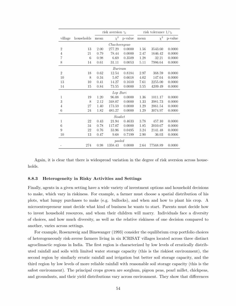
Again, it is clear that there is widespread variation in the degree of risk aversion across house-

holds.

8.8.3 Heterogeneity in Risky Activities and Settings

Finally, agents in a given setting have a wide variety of investment options and household decisions

to make, which vary in riskiness. For example, a farmer must choose a spatial distribution of his

plots, what lumpy purchases to make (e.g. bullocks), and when and how to plant his crop. A

microentrepreneur must decide what kind of business he wants to start. Parents must decide how

to invest household resources, and whom their children will marry. Individuals face a diversity

of choices, and how much diversity, as well as the relative riskiness of one decision compared to

another, varies across settings.

For example, Rosenzweig and Binswanger (1993) consider the equilibrium crop portfolio choices

of heterogeneously risk-averse farmers living in six ICRISAT villages located across three distinct

agroclimactic regions in India. The �rst region is characterized by low levels of erratically distrib-

uted rainfall and soils with limited water storage capacity (this is the riskiest environment), the

second region by similarly erratic rainfall and irrigation but better soil storage capacity, and the

third region by low levels of more reliable rainfall with reasonable soil storage capacity (this is the

safest environment). The principal crops grown are sorghum, pigeon peas, pearl millet, chickpeas,

and groundnuts, and their yield distributions vary across environment. They show that di¤erences

54

in risk aversion do translate into di¤erences in choice of risky investments. Individuals are in�u-

enced by risk-reduction when choosing income streams, particularly in response to limitations on

ex post consumption-smoothing, and the degree to which they are in�uenced depends on their risk

aversion.

Dercon (1996) also studies the variation in riskiness of agricultural investment decisions by

heterogeneously risk-averse rural households. His data is drawn from Tanzania, a country with very

underdeveloped credit markets (in 1989, only 5% of commercial bank lending went to the private

sector, and less than 10% of this lending went to individual farmers). The UN Food and Agriculture

Organization provides an interesting look at the vast heterogeneity in crop yield distributions and

equilibrium crop mix across regions in Tanzania in 1998. The following table shows the area,

yield, and production of each of �ve crops across ten agroclimactically heterogeneous regions in

Tanzania23:

Unfortunately, this table excludes estimates of the variance of yield of each of these crops across

regions. Dercon (1996) provides a discussion of this in his paper. He describes a multiplicity of soils

and irrigation systems in Tanzania, which support di¤erent crops. Paddy, a crop which can yield a

high return, is restricted only to speci�c soils and areas close to a river, and is the least drought and

locust resistant. Despite the potential for high returns, only 11% of the total cultivation sample

grew paddy. On the other hand, sorghum yields only a low-moderate return, but all soils can

sustain it, and it is more resistant to drought and pests. Even though it had a lower mean return,

it was grown by all but two households in the sample.

Uganda and Ethiopia are similar to Tanzania in the set of crops grown, though the actual

crop mix grown di¤ers due to di¤erences in environmental conditions. An IFPRI report from 2011

estimating crop yields in Uganda provides a useful illustration of how the variance of crop yields

di¤ers across crops, and the typical relationship of the variance with the mean:

23Of course, in addition to levels and �uctuations of crop yields, farmers care about the levels and �uctuations ofcrop prices, as they care ultimately about the distribution of pro�ts.

55

There is a clear positive relationship between mean yield and variance of yield. Groundnuts

have low mean yields and correspondingly low �uctuation of yields, making it a "safer" crop, while

banana has much higher mean yields but correspondingly higher �uctuation of yields, making it a

"riskier" crop.

Abebe et. al. (2010) provide a similar graphic for Ethiopia:

(Enset is a type of banana.)

Again, we get a general sense that higher mean yield crops have a higher variance of yield, while

lower mean yield crops have a smaller variance of yield. Comparing across Uganda and Ethiopia,

56

we see that maize is a safer crop relative to sweet potato in Uganda, but the opposite is true in

Ethiopia. Thus, the same set of crops have very di¤erent yield distributions in di¤erent settings,

and furthermore, each crop�s relative riskiness with the other crops also varies across setting.

57