endogenous leverage and expected stock returnsendogenous leverage and expected stock returns ... one...

Finance Research Letters xxx (2011) xxx–xxx

Contents lists available at ScienceDirect

Finance Research Letters

journal homepage: www.elsevier .com/locate/fr l

Endogenous leverage and expected stock returns

T.C. Johnson ⇑, T. Chebonenko, I. Cunha, F. D’Almeida, X. SpencerDepartment of Finance, University of Illinois at Urbana-Champaign, United States

a r t i c l e i n f o a b s t r a c t

Article history:Received 20 August 2010Accepted 24 December 2010Available online xxxx

Jel classifications:D92G10G12G32

Keywords:Expected stock returnsOptimal capital structure

1544-6123/$ - see front matter � 2010 Elsevier Indoi:10.1016/j.frl.2010.12.003

⇑ Corresponding author.E-mail address: [email protected] (T.C. Johnson).

Please cite this article in press as: Johnson, TResearch Letters (2011), doi:10.1016/j.frl.201

This note clarifies conditions under which endogenous choice ofdebt induces a negative relation between leverage or default riskand expected stock returns. In the context of the model of Georgeand Hwang [2009. Journal of Financial Economics 96, 56–79], wecorrect the contention that variation in bankruptcy costs acrossfirms is sufficient. Variation in asset risk parameters can lead tothe desired relation, but may not when also controlling for varia-tion in book-to-market ratios. A simple parameterization ofcross-sectional heterogeneity in risk and profitability implies anegative association of expected return with leverage and distressrisk and a positive association with book-to-market.

� 2010 Elsevier Inc. All rights reserved.

1. Introduction

Does the endogeneity of firm debt explain the negative cross-sectional relation observed in thedata between stock returns and leverage or default risk? A recent paper by George and Hwang(2009) asserts that capital structure optimization by firms which differ in their expected bankruptcycosts may yield such an association. If true, the hypothesis would nicely account for some puzzlingand much debated findings that seem to fly in the face of the intuition that higher debt should amplifysystematic risk exposures and so entail higher expected equity returns. More generally, their workspeaks to an important emerging theme in asset pricing: namely, that cross-sectional heterogeneityin business characteristics may account for some of the observed anomalies in the cross-section ofstock returns.

The model presented in their paper, however, does not support the proposed explanation for theleverage puzzle. Although their main proposition establishes that optimal debt does fall and expectedreturns do rise as costs of distress increase, for reasonable parameters the effect is very small. More

c. All rights reserved.

.C., et al. Endogenous leverage and expected stock returns. Finance0.12.003

http://dx.doi.org/10.1016/j.frl.2010.12.003

mailto:[email protected]


http://www.sciencedirect.com/science/journal/15446123

http://www.elsevier.com/locate/frl


2 T.C. Johnson et al. / Finance Research Letters xxx (2011) xxx–xxx

importantly, the expected returns in the proposition are firm returns (i.e. debt plus equity) not stockreturns. For equity, in fact, the model delivers the opposite result: as distress costs increase and opti-mal debt declines, expected stock returns fall. Since the empirical evidence pertains to (levered) stockreturns, the puzzles are not consistent with the model’s predictions.

This note shows, however, that the desired relationships can be restored by modifying the assumedheterogeneity. We show that, instead of differences in bankruptcy costs, differences in business riskare sufficient. Reasonable variation in risk can lead to strongly significant negative association be-tween book debt and equity risk premia. We thus verify the thrust of the conclusion of George andHwang (2009), that, in a world with diverse firms and endogenous levels of debt, the empirical find-ings may not be a puzzle.1

That is not the end of the story, though, because the empirical work in this area sets the bar higherthan merely delivering univariate relationships. In particular, it is much harder to reproduce the re-sults of regressions of returns on debt variables that also control for the ratio of equity book valueto market value. The book-to-market ratio summarizes the same risk characteristics captured byleverage. Further complicating things, distress risk and (book) debt levels may be negatively relatedin the model. Thus accounting for a negative return-distress risk finding is not merely a corollary ofa negative return-book debt relationship. In multiple regression, distress risk proxies may remain sig-nificantly negative in the presence of book debt.

Accounting for the desired multivariate associations requires heterogeneity along multiple dimen-sions. We show that the model can meet the challenge. We find that cross-sections that include var-iation in both asset risk and asset profitability are able to reproduce most of the observedrelationships. Further, these relationships are robust to the inclusion of moderate exogenous variationin debt induced by slow updating of firm capital structures. While we do not claim that the modelimplies that these findings must hold in general, the parameter heterogeneity we impose does notappear implausible in terms of implied observable firm characteristics.

The results underscore the importance of accounting for both differences in business characteris-tics and optimal firm policy choice in seeking to understand the cross-section of stock returns. InSection 2 we present a generalized version of the George and Hwang (2009) model. Section 3 analyzesthe induced relationships between debt and expected equity returns as firm characteristics vary. Sec-tion 4 shows how multidimensional heterogeneity can resolve the empirical puzzles, and assesses thesensitivity of the explanation to the assumption of ‘‘purely’’ endogenous capital structure. A final sec-tion summarizes the implications of the work and concludes.

2. The model

We consider a somewhat more general version of the model of George and Hwang (2009). Whilestill simplistic, the model is very tractable and allows for a transparent analysis of the capital structuredecision and its relation to expected returns.

The model envisions a cross-section of N finite-horizon firms, each having payoffs similar to thosein the familiar Merton (1974) model, but in which debt levels are chosen endogenously to trade offdistress costs and tax benefits.

The nth firm makes a one-time capital structure choice at the time of its birth, tðnÞ0 , to issue anamount K(n) P 0 of zero-coupon debt maturing at a time horizon tðnÞ2 . At that time, the firm will receivea lognormal payoff, V ðnÞ

tðnÞ2

, from its operations, and will then liquidate. We normalize the initial value ofthe payoff process to be V ðnÞ

tðnÞ0

¼ 1 for all n and interpret this as the book value of assets. There are nocash-flows to (or from) investors between birth and liquidation. Nor is the firm permitted to adjust theamount of debt outstanding.

The cross-section of firms is observed at a common time t1 with tðnÞ0 6 t1 6 tðnÞ2 for all n. The modelthus encompasses the possibility that firms are not all observed at their optimum capital structure, in

1 Other rational explanations for a negative distress risk premium include that of Garlappi et al. (2008) based on the possibilityof cash extraction by equity holders in bankruptcy, and O’Doherty (2010) based on increases in information uncertainty thatcoincide with distress.

Please cite this article in press as: Johnson, T.C., et al. Endogenous leverage and expected stock returns. FinanceResearch Letters (2011), doi:10.1016/j.frl.2010.12.003


0 0.5 1 1.50

0.05

0.1

0.15

0.2

0.25

K = eD

τ (K)

−4 −3 −2 −1 0 10

0.05

0.1

0.15

0.2

0.25

D = log(K)

τ (D)

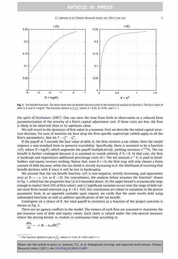
Fig. 1. Tax benefit function. The plots show the tax benefit function used in the numerical analysis in Section 3. The face value ofdebt is K and D = log(K). The function shown is A KC

BþKC where A = 0.25, B = 0.05, and C = 1.

T.C. Johnson et al. / Finance Research Letters xxx (2011) xxx–xxx 3

the spirit of Strebulaev (2007). One can view the time from birth to observation as a reduced formparameterization of the severity of a firm’s capital adjustment cost: if those costs are low, the firmis likely to be observed close to its optimum value.

We will revert to the dynamics of firm value in a moment. First we describe the initial capital struc-ture decision. For ease of notation we here drop the firm-specific superscript (which apply to all thefirm’s parameters). Also let T ¼ tðnÞ2 � tðnÞ0 .

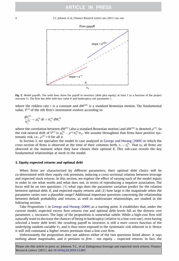
If the payoff at T exceeds the face value of debt, K, the firm receives a tax rebate. Here the modelimposes a non-standard form to preserve tractability. Specifically, there is assumed to be a functions(D), where D = log(K), which augments the payoff multiplicatively, yielding investors es(D)VT. The taxbenefit is further contingent because it is assumed to vanish entirely if VT < K. In that case, the firmis bankrupt and experiences additional percentage costs of c. The net amount e�c VT is paid to bond-holders and equity receives nothing. Notice that, even if c = 0, the firm may still only choose a finiteamount of debt because, while the tax shield is strictly increasing in K, the likelihood of receiving thatbenefit declines with K since it will be lost in bankruptcy.

We assume that the tax benefit function s(D) is non-negative, strictly increasing, and approacheszero as D ? �1 (i.e. as K ? 0). For concreteness, the analysis below assumes the function2 shownin Fig. 1, which has the properties that (a) it is bounded above; (b) the upper bound is economically largeenough to matter (here 25% of firm value); and (c) significant variation occurs over the range of debt val-ues most firms would entertain (e.g. K = 0.1–0.9). Our conclusions are robust to variations in the preciseparametric form. In an appendix available upon request, we verify that the same results hold usingunbounded functions as well as additive specifications of the tax benefit.

Contingent on a choice of K, the total payoff to investors as a function of the project outcome isshown in Fig. 2.

There are no agency conflicts in the model. The owners of each firm are assumed to maximize thepre-issuance sum of debt and equity values. Each claim is valued under the risk-neutral measure,where the pricing kernel, m, evolves in continuous-time according to

2 The

PleaseResea

dmt

mt¼ �r dt � rmdW ðmÞ

t

function plotted is just A KC

BþKC where A = 0.25, B = 0.05, and C = 1.

cite this article in press as: Johnson, T.C., et al. Endogenous leverage and expected stock returns. Financerch Letters (2011), doi:10.1016/j.frl.2010.12.003


Firm payoff

K

slope = eτ(D)

slope = e−c

VT

Fig. 2. Model payoffs. The solid lines show the payoff to investors (debt plus equity) at time T as a function of the projectoutcome VT. The firm has debt with face value K and bankruptcy cost parameter c.


where the riskless rate r is a constant and dW(m) is a standard Brownian motion. The fundamentalvalue, V(n) of the nth firm’s investment evolves according to

PleaseResear

dV ðnÞt

V ðnÞt

¼ lðnÞa dt þ rðnÞa dW ðnÞt

where the correlation between dW(n) (also a standard Brownian motion) and dW(m) is denoted q(n). Sothe risk-neutral drift of V(n) is lðnÞa � qðnÞrðnÞa rm. We assume throughout that firms have positive sys-tematic risk, i.e., q(n) > 0 for all n.

In Section 3, we specialize the model to case analyzed in George and Hwang (2009) in which thecross-section of firms is observed at the time of their common birth, t1 ¼ tðnÞ0 . That is, all firms areobserved at the moment when they have chosen their optimal K. This sub-case reveals the keyfundamental relationships at work in the model.

3. Equity expected returns and optimal debt

When firms are characterized by different parameters, their optimal debt choice will beco-determined with their equity risk premium, inducing a cross-sectional relation between leverageand expected stock returns. In this section, we explore the effect of varying each of the model inputsin order to see what works and what does not, in terms of reproducing a negative association. Thefocus will be on two questions: (1) what sign does the parameter variation predict for the relationbetween optimal debt, K, and expected equity returns and (2) how large is the magnitude when theparameter varies over a plausible range? Additional important questions concerning the relationshipbetween default probability and returns, as well as multivariate relationships, are studied in thefollowing section.

Take Proposition 1 in George and Hwang (2009) as a starting point. It establishes that, under thecurrent model, expected excess firm returns rise and optimal debt levels fall as the distress costparameter, c, increases. The logic of the proposition is somewhat subtle. While a high-cost firm willnaturally want to decrease the chances of being in bankruptcy (relative to a low-cost one), even havingselected a lower debt level, the resulting payoff to investors is still a more convex function of theunderlying random variable VT, and is thus more exposed to the systematic risk inherent in it. Henceit will still command a higher return premium than a low-cost firm.

Unfortunately the proposition does not address either of the two questions listed above: it saysnothing about magnitudes, and it pertains to firm – not equity – expected returns. In fact, the

cite this article in press as: Johnson, T.C., et al. Endogenous leverage and expected stock returns. Financech Letters (2011), doi:10.1016/j.frl.2010.12.003



conclusions of the proposition are strongly reversed when equity expected returns are considered in-stead of firm returns.

Fig. 3 shows a typical case (parameters are given in the figure caption). If pE represents the equityrisk premium, then dpE

dc ¼@pE@K

@K�

@c þ@pE@c . The last term is zero because the distress costs are borne entirely

by debt holders in default, so there is no direct effect of c on equity payoffs at all. The proposition

0 0.1 0.2 0.3 0.40.51

0.52

0.53

0.54

0.55

0.56

0.57

0.58

0.59

0.6

distress costs (c)

optimal debt (K*)

0 0.1 0.2 0.3 0.40.069

0.07

0.071

0.072

0.073

0.074

distress costs (c)

equity risk premium

0 0.1 0.2 0.3 0.4

0.0505

0.0505

0.0505

0.0505

0.0505

0.0505

0.0506

0.0506

distress costs (c)

firm risk premium

Fig. 3. The effect of varying bankruptcy costs. The figure shows optimal debt (left), expected excess returns to equity (center)and expected excess returns to debt plus equity (right) as a function of the parameter c. The plots set r = 0.05, rm = 0.50, T = 4,la = 0.12, ra = 0.20, and q = 0.50. The tax function parameters are given in the caption to Fig. 1.

0 0.1 0.2 0.3

0.35

0.4

0.45

0.5

0.55

0.6

main tax benefit parameter (A)

optimal debt (K)

c=0.1c=0.2c=0.3

0 0.1 0.2 0.30.067

0.068

0.069

0.07

0.071

0.072

0.073

0.074

0.075

0.076

main tax benefit parameter (A)

equity risk premium

c=0.1c=0.2c=0.3

Fig. 4. The effect of varying tax benefits. The figure shows optimal debt (left) and expected excess returns to equity (right) as afunction of the parameter A. The plots set r = 0.05, rm = 0.50, T = 4, la = 0.12, ra = 0.20, and q = 0.50. Three values of thebankruptcy cost parameter c are shown. The tax function parameters are given in the caption to Fig. 1.



0 0.1 0.2 0.3 0.4 0.50.2

0.4

0.6

0.8

1

1.2optimal debt (K*)

optimal debt (K*)

0 0.1 0.2 0.3 0.4 0.50.02

0.04

0.06

0.08

0.1

0.12

0.14

0.16

asset risk (σa) asset risk (σa)

equity risk premium

0 0.2 0.4 0.6 0.8 10.45

0.5

0.55

0.6

0.65

0 0.2 0.4 0.6 0.8 10

0.02

0.04

0.06

0.08

0.1

0.12

0.14

asset exposure (ρ) asset exposure (ρ)

equity risk premium

Fig. 5. The effect of varying asset risk. The figure shows optimal debt (left), expected excess returns to equity (right) as afunction of firm risk parameters. The top panels vary ra while fixing q = 0.50. The bottom panels vary q while fixing ra = 0.20.All panels use r = 0.05, rm = 0.50, T = 4, la = 0.12, c = 0.20. The tax function parameters are given in the caption to Fig. 1.


shows @K�

@c < 0, and @pE@K > 0 is just the standard levering effect of debt. High cost firms which choose

lower leverage will thus have safer equity and lower risk premia.3

The right panel of Fig. 3 shows a second difficulty with invoking heterogenous distress cost to solvestock expected return puzzles. The magnitude of the induced variation in firm risk premia is too smallto be likely to be discernible in empirical tests, even with c running from 0% to 50% of firm value. Intu-itively, marginal variations in systematic payoff risk induced through changes in deadweight costs inthe future are simply not large enough to have much effect on the firm’s overall risk profile.

Now consider the effect of varying the other ingredient in the firm’s trade-off calculation: tax ben-efits. The parameter A controls the magnitude of maximal tax shield, scaling up or down the functionplotted in Fig. 1. When varying A as shown in Fig. 4, we see, as expected, that higher tax benefits

3 Following George and Hwang (2009), the graphs in this section (with one exception) compute the expected equity returns asthe log of the equity expected payoff over the price of equity, divided by T. That is, these are T-horizon expected returns. Usinginstead instantaneous expected returns does not alter any of the conclusions in the analysis.



0 0.05 0.1 0.15 0.20.35

0.4

0.45

0.5

0.55

0.6

0.65

0.7

0.75

asset growth (μa) asset growth (μa)

optimal debt (K)

0 0.05 0.1 0.15 0.20.0695

0.07

0.0705

0.071

0.0715

0.072

0.0725

0.073

0.0735

0.074equity risk premium

Fig. 6. The effect of varying asset growth. The figure shows optimal debt (left), expected excess returns to equity (right) as afunction of the parameter la. The plots set r = 0.05, rm = 0.50, T = 4, c = 0.25, ra = 0.20, and q = 0.50. The tax function parametersare given in the caption to Fig. 1.


always induce higher debt. However, now there is a non-monotonic relation with expected equity re-turns. When A is greater than approximately 0.10, the equity risk premium has a negative relationshipwith debt. For lower tax rate firms, the relationship goes the opposite direction.4

In either case, the effects are not large: at most about 50 basis points per year over the range of Ashown. Moreover, other parameter sets can cause the changeover point (from positive to negativeslope of equity returns) to shift. Taken together, then, it seems unlikely (especially considering thepositive association induced by c) that cross-firm variation in trade-off parameters accounts for theobserved negative debt-stock return relation.

Following the intuition that we need riskier firms to choose less debt, the next natural thing to tryis simply to vary firms’ underlying risk. One can raise risk in the model either by increasing ra holdingq fixed (which increases systematic and idiosyncratic risk proportionally) or holding ra fixed andincreasing q (which trades off idiosyncratic for systematic risk). Fig. 5 shows that both mechanismswork.

Under this model, high asset-risk firms will choose low debt, but will remain riskier – even in theirequity – than low asset-risk firms with more debt. This finding is revealing. Not only might variation inasset risk account for a negative relation between stock returns and leverage, the plots indicate thathere the magnitudes can be very large. We will explore this as a potentially realistic explanationfor empirical results in Section 4.

Last, we consider the implications of varying the remaining parameters la and T. While not affect-ing asset risk, these quantities may influence risk premia via their role in determining bankruptcyprobabilities.

When varying la, the asset growth rate (or earnings), we do observe an induced negative relationbetween optimal debt and expected returns. See Fig. 6. Debt rises with la (since tax benefits are moredesirable for more profitable firms), yet expected stock returns fall. This is entirely due to the directchannel: @pE

@la< 0. Holding K fixed, higher growth de-levers the firm by increasing the value of equity.

4 Results in Graham (1996) indicate that the distribution of marginal tax rates is bimodal with a substantial mass (around 20%)of observations at zero.



0 2 5 7 10 15 200

1

2

3

4

5

6

7

8

9

debt maturity (T)

firm value

μ a =0.2

μ a=0.1

μ a =0.01

0 2 5 7 10 15 200

0.5

1

1.5

2

2.5

3

debt maturity (T)

optimal debt (K)

μ a =0.2

μ a=0.1

μ a =0.01

0 2 5 7 10 15 200.05

0.06

0.07

0.08

0.09

0.1

0.11

debt maturity (T)

equity risk premium

μ a =0.2

μ a=0.1

μ a=0.01

Fig. 7. The effect of debt maturity. The figure shows total firm value (debt + equity) (left), optimal debt (center) and expectedinstantaneous excess returns to equity (right) as a function of the parameter T. The plots set r = 0.05,rm = 0.50, c = 0.25,ra = 0.20, and q = 0.50. The tax function parameters are given in the caption to Fig. 1.


While the net effect is not large, it may be empirically important, as firms clearly do differ in their re-turn on assets.

Things are a little more complicated when we consider varying the firm’s liquidation date (and debtmaturity) T. Consider first the case where total firm value is not affected by T, which happens when therisk-neutral drift of V is equal to the riskless rate, r. An example is shown in the middle line (circles)in Fig. 7. In this case, the optimal level of debt is essentially unchanged with T. However, since therisk-neutral drift is still positive, there is again a de-levering effect from equity value increasing withT (as when la is raised). This produces a decline in equity risk and risk premium with T, shown in theright panel. Because K is essentially flat, there is no induced relation between T and the expectedreturns.5

When the risk-neutral growth rate exceeds the riskless rate (see the solid line in the figure), there isthe same de-leveraging effect, but also a strong increase in K with T since the firm can increase debtwithout incurring higher risk of default and because there is more to be gained from tax benefits. Thede-levering from the valuation channel is strong enough to dominate the direct levering from in-creased K. This produces a strong negative association between debt and equity expected returns.

Finally, for slowly growing (or less profitable) firms, debt becomes riskier with T (and tax benefitsless valuable) and so optimal debt declines. In this case, the valuation channel works to raise equityrisk, since longer horizon firms have more (risk-neutral) probability of default. However the declinein K is the stronger effect. So, as with the other cases, equity expected returns fall with T. (See the dot-ted-line plots in the figure.) So now the induced relation with K is positive.

Considering the overall effect of heterogeneity in firm duration, the relationship between K and pE

will be ambiguous if (as seems likely) there are both firms with high and low risk-adjusted growthrates – which may either be due to growth rates themselves or their risk adjustment. The analysissuggests that this dimension of heterogeneity may indeed lead to some rich cross-section patternsin firm returns.6 However, for purposes of accounting for debt-related anomalies, it is not the moststraightforward channel.

5 To ensure that expected excess returns are comparable across firms with differing T, the plot shows the instantaneousexpected excess returns, instead of the T-horizon expected excess returns. See footnote 3. The instantaneous expected return isqrarmV 0E=VE , where VE = VE(Vt) is the value of equity.

6 A recent paper by Chen (forthcoming) illustrates that cross-sectional differences in cash-flow duration can account fordifferences in the magnitude of the value premium across size deciles.




The analysis here also illustrates that consideration of multidimensional heterogeneity greatlyenrich the possible relations that the model can deliver. We now show that some particularparameterizations can indeed account for the relationships reported in the data.

4. Resolving the puzzles

Having seen that heterogeneity in some of the model parameters can yield an endogenously neg-ative cross-sectional relationship between debt and expected equity returns, it is important to recog-nize that this alone does not constitute a sufficient explanation for the empirical puzzles. One reasonfor this is that a negative association between expected stock returns and book debt may not imply asimilar association with empirical measures of leverage or distress. Another reason is that empiricalstudies invariably include other controls which may already capture the heterogeneity.

Specifically, consider the simultaneous relationship between leverage and book-to-market values.High-risk firms will not only have low (book) debt, they will also have low equity values. The equitybook-to-market ratio will summarize the firm’s risk-adjusted cost of capital, which takes into accountthe degree of leverage. There thus may be no independent role for debt in explaining equity returns.The puzzles are not about univariate associations. We now demonstrate that multivariate heterogene-ity in the model can meet this multivariate challenge.

To break the strong association between book-to-market and expected returns requires additionaldimensions of variation in firm parameters that lead to variations more strongly in one characteristicthan the other. A natural candidate is firm profitability, which will be reflected in valuation multipleswithout affecting asset risk exposures. However, it is not obvious whether this will be sufficient, sincerising profitability will also lead the firm to optimally choose higher leverage.

Fig. 8 shows how debt, book-to-market, and expected stock returns vary as joint functions of la andra.7 There is clearly a strong negative association between debt and returns. There is also a strong neg-ative relation between debt and the book-to-market ratio (BE/ME), but now BE/ME is less clearly linked toexpected returns.

Table 1 uses cross-sectional regressions to summarize the model implied joint relationship when aset of diverse firms is observed at the time of their optimization. A simulated cross-section of 4000independent firms is sampled having la and ra drawn from independent uniform distributions overthe ranges [0.00, 0.15] and [0.05, 0.45], respectively. The resulting optimal debt levels and BE/MEare then used as independent variables in a regression whose dependent variable is the expected ex-cess return to equity.8

With this specification, there is indeed a significant negative role for debt in explaining equity riskpremia, even controlling for book-to-market. In fact, the relationship is so strong when book debt, BD,itself is an independent variable that the remaining role for BE/ME is (counterfactually) negative. Ineffect, the regression is using this variable to clean up the nonlinearity in the debt relation. Substitut-ing market leverage, MD/ME, for BD restores the correct positive sign on the book-to-market ratio, asshown in the second column. The regression in column 3 follows George and Hwang (2009) and usesdummy variables for firms in the top and bottom quintiles of book debt, which achieves the sameresult.

A further challenge to the model is to explain the distress-risk puzzle, i.e., to reproduce the negativerelationship between expected stock returns and measures of credit risk or default probability. It isimportant to recognize that this is a distinct goal: in the model, it is not the case that high book debtvalues coincide with high credit risk. The optimal level of debt to issue is very sensitive to the valuethat will be realized when it is sold, which drops rapidly with default risk. For most parameterizations,this leads to an inverse relation between debt and credit risk.

7 We define ‘‘book equity’’ as cost of assets – which is 1 for all firms – minus face value of debt. Since the debt has zero coupon,one could argue that the ‘‘book value’’ of debt should be its present value, with book equity adjusted accordingly. The results beloware not sensitive to this alternative definition.

8 Note that this regression does not mimic empirical work in that we use the true expected return on the left-hand side, notobserved (noisy) returns. The t statistics in the table are thus not comparable to those using real data. They can be viewed as ameasure of the relative contribution of each variable in the regressions.



Table 1Expected return regressions with two-dimensional variation.

Variable 1 2 3

Book-to-market �0.0305 0.0229 0.0163(21.7) (30.2) (11.2)

Book debt �0.1843(74.1)

Market leverage �0.0852(82.2)

High debt �0.0352(34.3)

Low debt 0.0279(28.2)

The table shows the results of OLS regressions of expected excess returns to equity on firm-specificcharacteristics based on a sample of 4000 firms in which la and ra are drawn from independentuniform distributions over the ranges [0.00, 0.15] and [0.05, 0.45], respectively. The numbers inparentheses are OLS t statistics. Firms are assumed to be observed at the time of optimization. Thevariables ‘‘high debt’’ and ‘‘low debt’’ are dummies for whether book debt is in the top or bottomquintile of firms in the sample. The parameters common to all firms are r = 0.05, rm = 0.50, T = 4,c = 0.20, and q = 0.5. The tax function parameters are given in the caption to Fig. 1.

00.2

0.40

0.1

0.20

0.5

1

1.5

2

σa

optimal debt (K*)

μa 00.2

0.40

0.1

0.20

0.05

0.1

0.15

0.2

σa

equity risk premium

μa 00.2

0.4

0

0.1

0.2−1

0

1

2

σa

book equity/ market equity

μa

Fig. 8. Simultaneous variation in risk and profitability. The figure shows optimal debt (left), expected excess returns to equity(center) and the ratio of book-to-market equity (right) as a function of la and ra. All panels use r = 0.05, rm = 0.50, T = 4, c = 0.20,and q = 0.50. The tax function parameters are given in the caption to Fig. 1.


Addressing the credit-risk and debt level findings simultaneously requires introducing anotherdegree of variation in the cross-section of firms. Table 2 shows regression results from a simulatedsample of firms whose profitability, systematic risk, and idiosyncratic risk all vary. (Specifically,the sample draws la, ra, and q from independent uniform distributions over ranges [0.0, 0.20],[0.05, 0.35], and [0.10, 0.90], respectively.) As in the earlier sample, the regression reproduces apositive relationship with BE/ME and negative one with BD. In addition, credit risk, as measured byEDF (the probability of the firm defaulting) has a significantly negative relationship with expectedstock returns. The latter is not subsumed by book leverage,9 but constitutes a third dimension ofvariation in the cross-section.

9 George and Hwang (2009) find that some proxies for default risk are rendered insignificant when controlling for book debt.




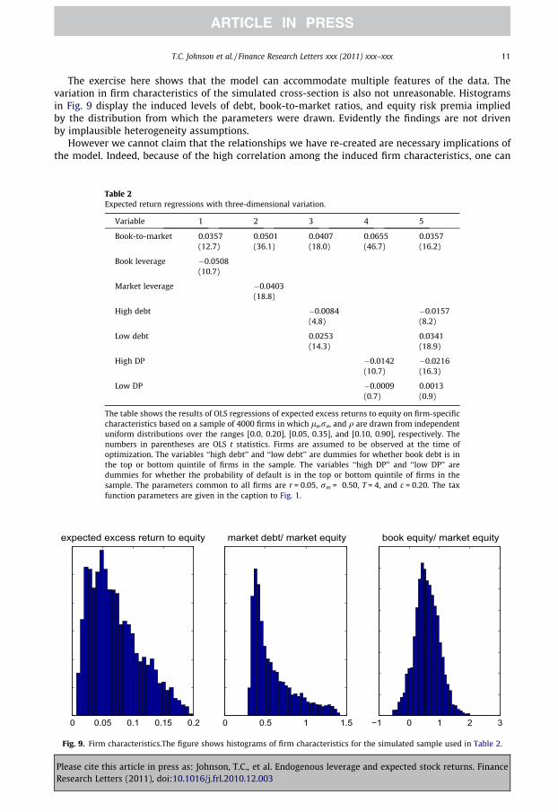
The exercise here shows that the model can accommodate multiple features of the data. Thevariation in firm characteristics of the simulated cross-section is also not unreasonable. Histogramsin Fig. 9 display the induced levels of debt, book-to-market ratios, and equity risk premia impliedby the distribution from which the parameters were drawn. Evidently the findings are not drivenby implausible heterogeneity assumptions.

However we cannot claim that the relationships we have re-created are necessary implications ofthe model. Indeed, because of the high correlation among the induced firm characteristics, one can

Table 2Expected return regressions with three-dimensional variation.

Variable 1 2 3 4 5

Book-to-market 0.0357 0.0501 0.0407 0.0655 0.0357(12.7) (36.1) (18.0) (46.7) (16.2)

Book leverage �0.0508(10.7)


High debt �0.0084 �0.0157(4.8) (8.2)

Low debt 0.0253 0.0341(14.3) (18.9)

High DP �0.0142 �0.0216(10.7) (16.3)

Low DP �0.0009 0.0013(0.7) (0.9)

The table shows the results of OLS regressions of expected excess returns to equity on firm-specificcharacteristics based on a sample of 4000 firms in which la,ra, and q are drawn from independentuniform distributions over the ranges [0.0, 0.20], [0.05, 0.35], and [0.10, 0.90], respectively. Thenumbers in parentheses are OLS t statistics. Firms are assumed to be observed at the time ofoptimization. The variables ‘‘high debt’’ and ‘‘low debt’’ are dummies for whether book debt is inthe top or bottom quintile of firms in the sample. The variables ‘‘high DP’’ and ‘‘low DP’’ aredummies for whether the probability of default is in the top or bottom quintile of firms in thesample. The parameters common to all firms are r = 0.05, rm = 0.50, T = 4, and c = 0.20. The taxfunction parameters are given in the caption to Fig. 1.

0 0.05 0.1 0.15 0.2

expected excess return to equity

0 0.5 1 1.5

market debt/ market equity

−1 0 1 2 3

book equity/ market equity

Fig. 9. Firm characteristics.The figure shows histograms of firm characteristics for the simulated sample used in Table 2.



0 0.5 1 1.5 20.1

0.15

0.2

0.25eq

uity

risk

pre

miu

m

book leverage

0 0.5 1 1.5 20.1

0.15

0.2

0.25

market leverage

Fig. 10. Exogenous vs endogenous leverage variation. The dotted-lines show the equity risk premium versus book leverage andmarket leverage for a sample of 4000 identical firms that are born at different times, tðnÞ0 , and observed at a common time, t1,when all have T = 4 years to maturity. The time length t1 � tðnÞ0 is drawn from an exponential distribution with mean 2.0. Thecircles to the lower left of each panel show the relationship when all firms are observed at birth. All firms have la = 0.15,ra = 0.2, q = 0.5, c = 0.2.


cause many of the regression coefficients to switch signs using sample designs that also seemdefensible. Based on numerical exploration of the three-dimensional variation used in Table 2, gettingall the correct relationships to be significant in specification 5, for example, appears to require that thesample contains both low growth firms (la < 0.05) and low correlation firms (q < 0.25).

One dimension of generality that we can readily check is the sensitivity of the results to theassumption that firms are observed precisely at the time of optimization. This assumption effectivelymaximizes the endogeneity of debt, which is clearly the driving force behind our findings. However, asemphasized in the dynamic capital structure literature (e.g., Strebulaev (2007)), firms are in realityslow to re-optimize due to financing frictions. Thus some exogenous variation in debt seeps intothe cross-section.

Fig. 10 shows how this hurts our argument. We imagine a cross-section of otherwise identicalfirms, that each optimized at some time tðnÞ0 in the past, but which are now observed at a common timet1 at which their debt has 4 years remaining to maturity. We draw t1 � tðnÞ0 from an exponential distri-bution with mean 2.0 (years) and then draw the random subsequent changes in fundamental valueV ðnÞt over that interval. (All firms have V = 1 at birth, as before.) The plots show the relation betweenexpected equity returns and leverage (book and market values) both at the time of initial optimization(circles) and at the time of observation (dots). In the cross-section of firms at optimization there issome variation in expected returns, due to firms’ differing durations, but all are between 14% and15%. This variation is positively associated with market leverage, but negatively associated with bookleverage due to the endogeneity mechanism.10

At T1 however, when some time has passed, there is a wide variation in expected returns which(since the firms are otherwise equal and their parameters have not changed) can only be due todifferences in Vt/K: firms that experienced positive news have effectively de-levered, whereas effectiveleverage has increased strongly for bad-news firms. As a result of this exogenous variation (i.e.,unrelated to the firm’s initial choice) there is now a strong positive association between equity riskpremium and market and book leverage.

10 For this exercise, we interpret the ‘‘book’’ value of assets at the observation time to be the fundamental value Vt. Book leverageat t is defined as K/Vt, and book equity is Vt � K.



Table 3Cross-sections of off-optimum firms.

1 2 3 4 5

Panel ABook-to-market 0.0556 0.0569 0.0367 0.0614 0.0370

(21.2) (37.7) (15.5) (44.0) (15.3)



High debt �0.0127 �0.0109(7.1) (5.6)

Low debt 0.0277 0.0275(15.1) (14.3)

High DP 0.0037 �0.0016(2.7) (1.2)

Low DP �0.0070 �0.0049(5.0) (3.4)

Panel BBook-to-market 0.0360 0.0502 0.0143 0.0453 0.0172

(16.1) (32.3) (8.0) (39.5) (9.4)


Market leverage 0.0056(2.7)

High debt �0.0220 �0.0171(14.0) (10.1)

Low debt 0.0397 0.0368(24.4) (21.8)

High DP 0.0117 0.0030(8.3) (2.1)

Low DP �0.0158 �0.0097(11.1) (6.9)

The table shows the results of OLS regressions of expected excess returns to equity on firm-specific characteristics based on asamples of 4000 firms whose characteristics are given in the caption to Table 2. In the Panel A, the time since optimization isexponentially distributed with mean 1.0. In the Panel B, the time since optimization is exponentially distributed with mean 2.0.


The cross-sections we generated above for Table 2 had substantially stronger endogenous leverageeffects than the one in this figure. But clearly if enough time has gone by since optimization, they toowill be characterized mostly by exogenous leverage variation, and the negative association withexpected returns will be lost. The question is how much time is too much.

Table 3 repeats the regression tests in Table 2 when we let the time since optimization be exponen-tially distributed with means 1.0 (Panel A) and 2.0 (Panel B). For purposes of comparison, we leave thesample size unchanged at 4000.

The table reveals that the negative relation between book leverage and expected returns(controlling for book-to-market) is remarkably robust, and survives even in the second panel wherethe expected lag since optimization is 2 years. The negative relation with market leverage surviveswith one year of expected observation lag, but not with two. Both cross-sections lose the desiredrelationship with the default probability indicators. Still, it is fair to conclude that the assertion thatthe major features of the debt puzzles may be explained by cross-sectional heterogeneity does notdepend strongly on the absence of any exogenous leverage variation.




5. Conclusion

We concur with George and Hwang (2009) that endogenous leverage choice and rational assetpricing may imply a negative and significant relation between debt (or leverage or distress risk)and expected equity returns. The model they propose offers a straightforward way to quantify theserelationships, which can be subtle, especially in the presence of related variables.

Using that model, we illustrate that heterogeneity in bankruptcy costs is not a sufficient condition.(In fact, the relationship with the equity risk premium goes the wrong way.) Variation in tax benefitsand in firm duration can, in certain circumstances deliver a negative association, but may also implythe opposite.

We show that simultaneous variation in firm profitability and risk can not only produce the desireddebt effects, but it can do so while controlling for differences in book-to-market ratios. When both sys-tematic and idiosyncratic risk vary, the model can also lead to a negative relation between defaultprobability and expected stock returns. The negative relations between equity expected returns andbook or market leverage are preserved when allowing for exogenous perturbation of leverage inducedby financing frictions.

To date, most rational asset pricing models that seek to explain cross-sectional patterns in observedreturns have not invoked firm heterogeneity. The alternative strategy has been to model firms that areex ante identical, but that experience differing histories of productivity shocks or investment opportu-nities. This approach has much to recommend it, and has yielded many insights, especially with regardto the dynamic evolution of firms’ risk profiles. (Obreja (2006) and Gomes and Schmid (2010) analyzethe leverage-return relationship in this general framework.) However, based on the analysis here, it isclear that also taking into account simple, static variation in cash-flow characteristics across differentbusiness types has great potential to add to our understanding of observed relationships between as-set returns and other company characteristics. An important challenge, moving forward, is to establishthe rules of the game for this type of exercise by parameterizing the actual joint distribution of assetcharacteristics.

Acknowledgment

We thank Dirk Hackbarth for advice and encouragement.

Appendix A. Supplementary material

Supplementary data associated with this article can be found, in the online version, at doi:10.1016/j.frl.2010.12.003.

References

Chen, Huafeng, forthcoming. Firm life expectancy and the heterogeneity of the book-to-market effect. Journal of FinancialEconomics.

Garlappi, Lorenzo, Shu, Tao, Yan, Hong, 2008. Default risk, shareholder advantage and stock returns. Review of Financial Studies81, 2743–2778.

George, Thomas J., Hwang, Chuan-Yang, 2009. A resolution of the distress risk and leverage puzzles in the cross section of stockreturns. Journal of Financial Economics 96, 56–79.

Gomes, Joao F., Schmid, Lukas, 2010. Levered returns. Journal of Finance 65, 467–494.Graham, John R., 1996. Debt and the marginal tax rate. Journal of Financial Economics 41, 41–73.Merton, Robert C., 1974. On the pricing of corporate debt: the risk structure of interest rates. Journal of Finance 29, 449–470.Obreja, Ilujan, 2006. Financial Leverage and the Cross-section of Stock Returns. Carnegie Mellon University Working Paper.O’Doherty, Michael S., 2010. Information Risk, Conditional Betas, and the Financial Distress Anomaly. University of Iowa

Working Paper.Strebulaev, Ilya A., 2007. Do tests of capital structure theory mean what they say? Journal of Finance 62, 1747–1787.





endogenous leverage and expected stock returnsendogenous leverage and expected stock returns ... one...

Documents