endosulfan, risk characterization document, volume · pdf fileendosulfan risk characterization...
TRANSCRIPT
ENDOSULFAN
RISK CHARACTERIZATION DOCUMENT
Volume III
Environmental Fate
Environmental Monitoring Branch Department of Pesticide Regulation
California Environmental Protection Agency
May 2008

Endosulfan Environmental Fate May 2008
2
ENDOSULFAN
RISK CHARACTERIZATION DOCUMENT
Volume III
Environmental Fate
Shifang Fan, Ph. D.
Department of Pesticide Regulation Environmental Monitoring Branch
P.O. Box 4015 Sacramento, California 95812-4015

Endosulfan Environmental Fate May 2008
3
Table of Contents Chemical structure characteristics and physicochemical properties..............................................5 Regulation......................................................................................................................................7 Use Profile in California ................................................................................................................8 Environment Fate.........................................................................................................................20
Fate and persistence in soil ......................................................................................................23 Adsorption and desorption...................................................................................................23 Runoff transportation and leaching .....................................................................................23 Volatilization and dust transportation .................................................................................25 Degradation .........................................................................................................................25
Fate and persistence in atmosphere..........................................................................................28 Volatilization from crop surface and soil solution ..............................................................28 Spray drift ............................................................................................................................29 Dust transportation ..............................................................................................................29 Degradation .........................................................................................................................30 Air concentrations................................................................................................................30
Fate and persistence in water/sediments ..................................................................................36 Spray drift and runoff transportation ..................................................................................36 Adsorption/desorption and volatilization ............................................................................37 Degradation and overall dissipation ...................................................................................37 Water concentrations in California .....................................................................................40
Regional and remote transportation .........................................................................................43 Fate and persistence in biota ....................................................................................................46
Reference .....................................................................................................................................47

Endosulfan Environmental Fate May 2008
4
List of Tables Table 1. Endosulfan identity ........................................................................................................5 Table 2. Physicochemical properties of endosulfan ....................................................................6 Table 3. Summary of pesticide application label rates for major product uses in California......9 Table 4. Reported endosulfan use in counties with mean annual use >1,000 pounds...............11 Table 5. Monthly reported endosulfan use from 1996 to 2005..................................................14 Table 6. Reported endosulfan use for crops with mean annual use >200 pounds .....................15 Table 7. Endosulfan losses via runoff and leaching in different conditions..............................24 Table 8. Comparison of plastic and vegetative mulches on runoff transportation of endosulfan
..............................................................................................................................................25 Table 9. Soil degradation half-lives .........................................................................................26 Table 10. Comparison of half-lives under aerobic and anaerobic conditions.............................28 Table 11. Summary of ARB’s application monitoring results (1997)........................................33 Table 12. ARB’s application monitoring results during each interval at each site.....................33 Table 13. Summary of ARB’s ambient monitoring results (1996).............................................34 Table 14. ARB’s ambient monitoring results at each site ..........................................................35 Table 15. Quantifiable α-endosulfan results during DPR ambient monitoring in 1985 .............36 Table 16. Summary of hydrolysis half-lives at different temperature and pH ...........................38 Table 17. Summary of surface water monitoring results for endosulfan in each year ...............41 Table 18. Summary of surface water monitoring results for endosulfan in each county with
positive detections................................................................................................................41 Table 19. Summary of endosulfan well water monitoring results (1984-2005) .........................42 Table 20. Summary of monitoring results from three studies in Sierra Nevada Mountains ......44
List of Figures
Figure 1. Chemical structures of endosulfan (source from PANNA, 2007)................................6 Figure 2. Reported endosulfan use from 1996 through 2005 (DPR PUR Database) ................11 Figure 3. Endosulfan use map....................................................................................................12 Figure 4. Comparison of endosulfan use during 1997 vs 2005 in the Central Valley...............13 Figure 5. Monthly reported endosulfan use (1996-2005) in the top six counties ......................14 Figure 6. Reported endosulfan use (1996-2005) on the main crops in the top six counties......16 Figure 7. Comparison of estimated percentile distribution for the pounds of individual
endosulfan application in 1997 vs 2005...............................................................................17 Figure 8. Comparison of estimated percentile distribution for the acreage of individual
endosulfan application in 1997 vs 2005...............................................................................18 Figure 9. Comparison of estimated percentile distribution for the rate of individual endosulfan
application in 1997 vs 2005 .................................................................................................19 Figure 10. Endosulfan degradation in soil and water (source: GFEA, 2004)..............................22

Endosulfan Environmental Fate May 2008
5
Chemical structure characteristics and physicochemical properties Endosulfan is a chlorinated hydrocarbon insecticide and acaricide in the class of chlorinated cyclodiene, a member of organochlorine family (Table 1). Its distinguishing feature is that it contains only one double bond, whereas the most of the cyclodiene class members contain two double bonds. The molecular structures of its two stereochemical isomers, α- and β-endosulfan are depicted in Figure 1. The α-isomer is asymmetric and exists as two twist chair forms. The β-isomer is symmetric. Isomerization was found to be favored from β- to α-endosulfan (Schmidt, et al., 2001; Walse, et al., 2003).
Table 1. Endosulfan identity
Common Name:
Endosulfan
Chemical Name: IUPAC Chemical Abstract
6, 7, 8, 9, 10, 10-hexachloro-1, 5, 5a, 6, 9, 9a-hexahydro-6, 9-methano-2, 4, 3-benzadioxathiepin 3-oxide 6, 9-methano-2, 4, 3-benzodioxathiepin-6, 7, 8, 9, 10, 10-hexachloro1, 5, 5, 6, 9, 9-hexahydro-3-oxide
Chemical Family Organochlorine
Trade Name:
Thiodan®, Thionex®
CAS Registry Number:
959-98-8 33213-65-9 115-29-7 1031-07-8
α-Endosulfan β-Endosulfan Technical endosulfan (a mixture of α- & β-isomer) Endosulfan sulfate
Molecular Formula:
C9H6Cl6O3S
Molecular Weight:
406.96

Endosulfan Environmental Fate May 2008
6
Figure 1. Chemical structures of endosulfan (source from PANNA, 2007)
α-endosulfan β-endosulfan Technical grade endosulfan is a diastereomeric mixture of roughly 70% α-isomer and 30% β-isomer (US EPA, 2002), along with impurities and degradation products. Pure endosulfan is a colorless crystal; but technical grade is brown in color, ranging from light to dark depending on impurities. Its odor is similar to hexachlorocyclopentadiene, sometimes mixed with sulfur dioxide. Selected physiochemical properties for the major endosulfan forms in the environment are listed in Table 2.
Table 2. Physicochemical properties of endosulfan*
α - isomer β - isomer Technical grade endosulfan
Endosulfan sulfate
Melting point (oC) 108-110 208-210 70-124 181-201 b Solubility (mg/L @25 oC) 0.33 b 0.32 b 0.33 a 0.22 b Vapor pressure (mm Hg, @25 oC) 3.0x10⁻⁶ 7.2x10⁻⁷ 1.0x10⁻⁵ 8.3 x10⁻⁹ b Bulk density (g/ml) 1.8 c Flammability Not flammable b Henry’s Law constant (atm m3 mol-1@ 25 oC)
4.9x10⁻⁶ d
1.3x10⁻⁴ b 1.2x10⁻⁶ d 2.1x10⁻⁵ b
1.6x10⁻⁵ d
Log Kow (pH 5.1) 4.6-4.7 b 4.3-4.8 b 4.5-5.7 Koc (cm3/g) 10600 13600 12,000 a Soil aerobic half-life (days) 19-33 b 42-58 b 31.6 a 100-150 b Soil anaerobic half-life (days) 148 a Hydrolysis half-life (days) 11 (pH 7) 19 (pH 7) 14.8 a Photolysis half-life (days) >200 b *Data in this table are from US EPA, 2002 except for denoted ones. aDPR chemical database (DPR, 2004). bGFEA, 2004. cFootprint, 2007. dCalculated from vapor pressure and solubility.

Endosulfan Environmental Fate May 2008
7
Endosulfan is a broad-spectrum non-systemic insecticide and acaricide with contact and stomach action. It is used to control sucking, chewing, and boring insects on a wide variety of vegetables, fruits, grains, cotton, and tea, as well as ornamental shrubs, vines, and trees (Tomlin, 1994). Formulations of endosulfan include emulsifiable concentrate, wettable powder, ultra-low volume (ULV) liquid, and smoke tablets. Endosulfan is compatible with many other pesticides and may be found in formulations with dimethoate, malathion, methomyl, monocrotophos, pirimicarb, triazophos, fenoprop, parathion, petroleum oils, and oxine-copper. It is not compatible with alkaline materials because it is vulnerable to hydrolysis (US EPA, 2002). Application of endosulfan can be made using groundboom sprayer, fixed-wing aircraft, through irrigation systems (chemigation), airblast sprayer, rights-of-way sprayer for landscape maintenance, low pressure handwand sprayer, high pressure handwand sprayer, backpack sprayer and dip treatments (US EPA, 2002). Regulation Endosulfan is classified in the U.S. Environmental Protection Agency (US EPA) toxicity category I (40 CFR 156.60-156.62). Pesticide labels for products containing endosulfan must bear the Signal Words “DANGER – POISON” or “DANGER” depending on formulation. US EPA has established a series of regulations for endosulfan applications since it was registered as a pesticide in the U.S. in 1954 to control agricultural insect and mite pests. In 1981 and 1982, a Registration Standard and a Guidance Document were issued for endosulfan requiring additional generic and product-specific data for the manufacturing products of the technical registrants (US EPA 2002). In 1988, Federal Insecticide, Fungicide, and Rodenticide Act (FIFRA) was amended to accelerate the reregistration of products with active ingredients registered prior to November 1, 1984 to ensure that they meet more stringent standards, and to report product information concerning unreasonable adverse effects to US EPA. In 1990, the Update Endosulfan Reregistration Standard was issued, which summarized regulatory conclusions based on available residue chemistry data and specified the additional data required for reregistration purposes. Between 1985 and 1994, eight data call-ins concerned potential formation of chlorinated dibenzo-p-dioxins and dibenzofurans and residue chemistry data deficiencies. In 1996, the Food Quality Protection Act (FQPA) amended and strengthened the standard for establishing tolerances under the Federal Food, Drug, and Cosmetic Act (FFDCA). To implement provisions of the FQPA of 1996, US EPA considered the special sensitivity of infants and children to pesticides, as well as aggregate exposure of the public to pesticide residues from all sources, and the cumulative effects of pesticides and other compounds with common mechanisms of toxicity. In November 2002, the reregistration eligibility decision (RED) concluded that agricultural uses of endosulfan based on approved labeling pose occupational risks of concern and ecological risks that constitute unreasonable adverse effects on the environment. However, these risks can likely be mitigated to levels below concern through changes to pesticide labeling and formulations. US EPA has determined that endosulfan is eligible for reregistration with conditions (1) additional required data will confirm this decision for occupational exposures associated with the application of dip treatment to roots or whole plants and ecological risks; and (2) the risk mitigation outlined in the RED are adopted, and label

Endosulfan Environmental Fate May 2008
8
amendments are made to reflect these measures. If vulnerable areas in specific geographic areas are identified as a result of the stakeholder process, additional ecological risk mitigation measures may be necessary to protect especially sensitive organisms (US EPA, 2002). In September 2006, US EPA revoked certain tolerances and is modifying and establishing new tolerances for endosulfan and other pesticides (US EPA, 2006a). In 1991 the federal technical registrants amended labels to incorporate a 300-foot spray drift buffer for aerial applications between treated areas and water bodies. This setback was adopted to address concerns about contamination of water and risks to aquatic organisms. In 2000, technical product labels were amended to remove all residential use patterns. The registrants have further restricted the annual maximum use rate to 3 pounds active ingredient per acre for all uses. In addition to the federal regulations, California amended its more stringent policies and regulation for endosulfan uses. Pursuant to Section 14004.5 of the Title 3, Food and Agricultural Code (FAC), endosulfan is designated a restricted use material in section 6400 (e) of the FAC with exceptions only for home, structural, industrial, institutional, or public agency vector control districts uses that are pursuant to section 2426 of the Health and Safety Code. Restricted materials are possessed and used by persons only under permit of the county agricultural commissioner. Pursuant to Section 13127 of the FAC, the Birth Defect Prevention Act (Statutes 1984, Chapter 669) mandates the listing of endosulfan in section 6198.5 of FAC. The 200 priority pesticide active ingredients listed in this section have the most significant data gaps and widespread use and are suspected to be hazardous to people. Currently, all data requirements for endosulfan have been submitted to the Department of Pesticide Regulation (DPR. 2007a). Pursuant to Section 13143 of the FAC, Pesticide Pollution Prevention Act (AB 2021) mandates data call-in of chemistry and environmental fate studies for products with active ingredient of endosulfan including degradation products in specific studies. Currently, all data requirements for endosulfan have been submitted to the Department of Pesticide Regulation (DPR. 2007a) Use Profile in California Endosulfan has been widely used in California. Currently, there are six products containing endosulfan as an active ingredient (a.i.) registered in California. Two emulsifiable concentrate insecticides (34% a.i.) and three wettable powder formulations (50% a.i.) are registered for agricultural or commercial use only. The other one is a technical insecticide (95% a.i.) for manufacture of insecticides and acaricides only. The registered endosulfan products are used to control aphids, thrips, beetles, foliar feeding larvae, leafminer, mites, borers, cutworms, fruitworms, bugs, whiteflies, leafhoppers, loopers, and weevils for a wide variety of fruit trees, vegetables, and other crops, such as apples, nectarines, peaches, prune, lettuce, tomatoes, cantaloupe, grapes, melons, vegetable peppers, broccoli, sugarbeet, cauliflower, carrots, cabbage, rape, squash, cucumber, strawberry, alfalfa, corn, potato, beans, cotton, walnut, pecan, etc. The

Endosulfan Environmental Fate May 2008
9
application rates vary depending on target crop, product used, and pest to be controlled. Labeled application rates are summarized in Table 3.
Table 3. Summary of pesticide application label rates for major product uses in California
Application Rates Crops Pests to be Controlled WP or WSB* EC** Apples, nectarines, peaches, prunes, and citrus
Aphids, mite, leafhopper, stink bugs, and borers
1 lb/100 gals or max. 8 lbs/acre
0.66qt/100 gals or max. 3.33 qts/acre
Lettuce, broccoli, cabbage, cauliflower, cucumbers, melons, squash, peppers, carrots, potatoes, sweet potatoes, strawberries, tomatoes, sugarbeets, and beans
Aphids, loopers, worms, whiteflies, moth larvae, beetles, leafhoppers, spittlebugs, stink bugs, and borers
1-2 lbs/acre 0.66-1.33 qts/acre
Alfalfa (for seed only) Spotted alfalfa aphid 2.66 pints/acre Strawberries Cyclamen mite, 4 lbs/acre in 400
gals water 2.66 qts/ acre in 400 gals water or 1.33-2 qts/ acre
Sweet corn (vegetable) Aphids, whiteflies Earworms
1.33 qts/acre 2 qts/acre
Grapes Leafhoppers, chafers 1 lb/100 gals or 2-3 lbs/acre
0.66 qt/100 gals or 1.5-2 qts/acre
Walnut Aphids 3-4 lbs/acre Pecans Spittlebug, aphid, and
nut casebearer 1.5 lb/100 gals max. 8 lbs/acre
1 qt/100 gals
Cotton Leaf perforator Aphids Worms, loopers, leafhoppers, lygus bugs, stink bugs, and thrips Whiteflies
2 lbs/acre
1.33-2 qts/acre 0.5-1 qt/acre 1.33-2 qts/acre 2 qts/acre 1.5 qts/acre
*Wettable Powder or Water Soluble Bags **Emulsifiable Concentrate DPR fully implemented agricultural pesticide use reporting system in 1990. All agricultural use must be reported monthly to the county agricultural commissioners. The county agricultural commissioners forward these data to DPR. DPR annually compiles the data and makes pesticide use reports available to the public. Agricultural use also includes applications to parks, golf courses, cemeteries, rangeland, pastures, and rights-of-way. Although use in structural pest control is excluded, the use of pesticides designated as restricted materials pursuant to section 14004.5 of the Food and Agricultural Code must be reported as non-agricultural use. For non-agricultural applications, detailed geographic information such as base meridian/township/range/

Endosulfan Environmental Fate May 2008
10
section is not provided. In this document, pesticide use data were queried from DPR’s database (DPR, 2007b) with exclusion of outliers (Wilhoit, 1998). In recent ten years, annual endosulfan use reported decreased from 238,635 pounds in 1997 to 83,242 pounds of active ingredient in 2005 (Figure 2) and average of the ten-year annual use was 161,056 pounds. Table 4 lists annual endosulfan use in the counties where the average annual use exceeded 1,000 pounds. The six top use counties where ten-year averages of annual use exceeded 6,000 pounds of active ingredient were Fresno, Kings, Kern, and Tulare in San Joaquin Valley, and Riverside and Imperial counties (Figure 3). A side-by-side comparison of the use maps for 1997 and 2005 show decreased endofulfan use in 2005, mainly due to reduction of cotton crop in the San Joaquin Valley (Figure 4). Endosulfan use on cotton decreased 87% in 2005 vs 1997 in the top six counties. Monthly use for the entire state showed that the peak use months were from June to September with some variations before year 2000 (Table 5). For the six top use counties, the peak use months were June to August in Fresno; June and July in Imperial; August and September in Kern; June to September in Kings; May to August in Riverside; and July to September in Tulare counties (Figure 5). In California, endosulfan was mainly used on cotton, alfalfa, lettuce, tomato, melons, grapes, and various vegetables in the years between 1996 and 2005 (Table 6). For the six top use counties, the main use crops were head lettuce, alfalfa, canning tomatoes, and cotton in Fresno; alfalfa in Imperial; cotton and alfalfa in Kings, and cotton in Kern, Riverside, and Tulare counties (Figure 6). A percentile comparison was performed to identify differences of individual endosulfan applications between 1997 and 2005. Although the absolute total pounds used and acreage applied in 2005 decreased to 1/3 of those in 1997, the individual application frequency distribution patterns for pounds used (Figure 7), acres applied (Figure 8), and application rates (Figure 9) were very similar. Generally, the relative differences of pounds used, acres applied, and application rates between 1997 and 2005 were less than 20% at each of five percentiles, 25, 50, 75, 90, and 95 (Figures 7-9), except for the pounds used (50%) and acres applied (40%) at 25 percentile (Figures 7 and 8). The top five crops for endosulfan use were cotton, alfalfa, lettuce head, canning tomato, and cantaloupe in both 1997 and 2005 (Table 6). It can be concluded that the use patterns of individual endosulfan applications were similar in 2005 compared to 1997.

Endosulfan Environmental Fate May 2008
11
Figure 2. Reported endosulfan use from 1996 through 2005 (DPR PUR Database)
Table 4. Reported endosulfan use in counties with mean annual use >1,000 pounds County 1996 1997 1998 1999 2000 2001 2002 2003 2004 2005 AverageFRESNO 75400 104405 89624 100057 85684 83103 57991 51658 52220 43482 74362KINGS 25296 49397 14181 18879 12883 9357 26293 20816 52302 14720 24412IMPERIAL 68431 31165 24346 18481 17515 14830 6575 12406 4879 7282 20591KERN 10125 21449 8917 4250 9399 25028 23534 26559 24750 2693 15670TULARE 8427 8272 3756 3603 3673 8590 11384 7862 8206 1097 6487RIVERSIDE 19956 9524 3394 2726 2604 2933 7605 8490 3046 4240 6452SAN BERNARDINO 1853 264 528 17288 175 15 9 2013MONTEREY 5007 3734 4438 2354 1609 224 140 1135 2 438 1908SAN BENITO 2828 2911 1001 3829 1743 783 1081 614 2019 142 1695YOLO 1143 359 900 1314 1593 1222 1193 1033 2265 2007 1303SOLANO 6 2033 1457 1710 1798 579 1051 1720 1036
0
50,000
100,000
150,000
200,000
250,000
1996 1997 1998 1999 2000 2001 2002 2003 2004 2005Year
Act
ive
ingr
edie
nt u
sed
(lbs)

Endosulfan Environmental Fate May 2008
12
Figure 3. Endosulfan use map

Endosulfan Environmental Fate May 2008
13
Figure 4. Comparison of endosulfan use during 1997 vs 2005 in the Central Valley

Endosulfan Environmental Fate May 2008
14
Table 5. Monthly reported endosulfan use from 1996 to 2005 Month 1996 1997 1998 1999 2000 2001 2002 2003 2004 2005 AverageJAN 4369 2894 780 3992 821 1921 1649 843 838 346 18453FEB 7001 7870 4257 4052 6901 7973 5797 6295 3094 4652 57891MAR 8328 14577 14549 13961 8775 8878 6292 5927 7508 6902 95697APR 10277 3904 5913 3248 2471 2840 6134 2078 849 691 38406MAY 26640 14471 1537 22861 3198 7175 6333 1385 3044 3540 90183JUN 37665 42264 17497 36382 42087 27737 13291 19147 14610 17205 267885JUL 62505 90059 59212 55005 43556 29720 18966 20443 21559 20913 421938AUG 33000 40342 29810 21653 20238 38742 26662 28355 48489 12797 300088SEP 8179 9325 12175 13016 11900 21020 45779 35884 42097 7793 207169OCT 12958 9430 8602 5478 4287 6906 10926 12617 10884 7387 89474NOV 7212 2630 813 647 266 270 422 655 302 332 13547DEC 5873 871 820 15 251 314 415 465 150 654 9828Total 224007 238635 155963 180311 144751 153497 142666 134093 153424 83212 1610559
Figure 5. Monthly reported endosulfan use (1996-2005) in the top six counties
0
50000
100000
150000
200000
250000
FRESNO IMPERIAL KERN KINGS RIVERSIDE TULARE
County
Act
ive
ingr
edie
nt u
sed
(lbs)
JAN
FEB
MAR
APR
MAY
JUN
JUL
AUG
SEP
OCT
NOV
DEC

Endosulfan Environmental Fate May 2008
15
Table 6. Reported endosulfan use for crops with mean annual use >200 pounds Commodity 1996 1997 1998 1999 2000 2001 2002 2003 2004 2005 MeanCOTTON 50525 91537 20784 7072 14136 44279 61320 58101 76638 11952 43634ALFALFA 16440 39436 59726 63634 53175 25758 10198 12334 9603 13446 30375LETTUCE, HEAD 24828 25839 22999 27922 17749 21133 15543 14833 17619 14444 20291TOMATOES (CANNING) 19154 9005 9762 21383 21613 20802 14360 23254 20174 19302 17881CANTALOUPE 42302 24988 12311 10631 11639 11800 8785 6927 9981 6053 14542LETTUCE, LEAF 5975 6007 6054 7171 4900 5602 5106 4728 4324 4357 5423GRAPES 9497 3767 2791 20799 3973 4310 2695 272 362 40 4851MELONS 8036 6671 2409 1741 2783 2952 2703 2672 1013 1561 3254BROCCOLI 4849 3322 5270 1958 1281 3326 2999 3590 3844 757 3120PEPPERS, VEGETABLE 4511 1845 628 1005 1178 3125 322 1215 3885 1378 1909CORN (HUMAN CONSUMPTION) 7001 1545 1306 1587 456 428 1839 319 274 1297 1605SUGARBEET 5647 3310 147 1259 1649 332 2607 252 1520WATERMELONS 3531 2403 374 991 959 888 2282 1615 1006 1096 1514POTATO 2553 1987 130 1611 576 686 3264 470 1324 776 1338TOMATO 2940 1388 1008 1981 2226 936 655 267 629 973 1300BEANS (DRIED-TYPE) 1498 1268 952 2192 350 373 1576 380 368 896WALNUT 3699 2408 286 636 358 287 30 80 707 81 857PEACH 186 1048 168 820 1116 1010 946 73 51 14 543CARROTS 607 1543 1075 205 163 644 129 374 474APPLE 376 1469 768 492 656 5 343 446 52 111 472CAULIFLOWER 910 701 570 683 494 485 256 112 50 25 429PECAN 756 823 782 460 222 270 180 143 594 423GRAPES, WINE 1093 749 731 376 23 103 465 135 103 378STRAWBERRY 663 47 10 140 10 14 406 2 2330 362PRUNE 262 188 851 175 513 222 492 329 187 298 352NECTARINE 36 312 63 220 318 395 1201 72 52 16 268RAPE 733 246 965 209 2 45 220SQUASH 237 499 19 322 344 208 212 27 173 24 207CABBAGE 555 260 275 195 118 234 30 145 118 109 204CUCUMBER 261 362 16 368 87 710 158 1 0 73 204

Endosulfan Environmental Fate May 2008
16
Figure 6. Reported endosulfan use (1996-2005) on the main crops in the top six counties
0
40000
80000
120000
160000
200000
FRESNO IMPERIAL KERN KINGS RIVERSIDE TULARE
County
Act
ive
ingr
edie
nt u
sed
(lbs)
COTTON
ALFALFA
LETTUCE HEAD
TOMATOES,CANNINGCANTALOUPE
LETTUCE, LEAF

Endosulfan Environmental Fate May 2008
17
Figure 7. Comparison of estimated percentile distribution for the pounds of individual endosulfan application in 1997 vs 2005
Pounds applied Relative difference (%) Percentile 1997 2005 (2005-1997)/average 25 12 20 50 50 26 30 14 75 56 66 16 90 116 120 3 95 148 150 1
0
20
40
60
80
100
120
0 500 1000 1500 2000 2500
Active Ingredient of Endosulfan Applied (pounds)
Perc
entil
e 19972005

Endosulfan Environmental Fate May 2008
18
Figure 8. Comparison of estimated percentile distribution for the acreage of individual endosulfan application in 1997 vs 2005
Acres applied Relative difference (%) Percentile 1997 2005 (2005-1997)/average
25 16 24 40 50 32 35 9 75 70 71 1 90 148 150 1 95 160 156 -3
0
20
40
60
80
100
120
0 100 200 300 400 500 600 700
Acreage Applied (acre)
Perc
entil
e 19972005

Endosulfan Environmental Fate May 2008
19
Figure 9. Comparison of estimated percentile distribution for the rate of individual endosulfan application in 1997 vs 2005
Application rate (pounds/acre) Relative difference (%) Percentile 1997 2005 (2005-1997)/average 25 0.75 0.75 0 50 0.80 0.93 15 75 1.00 1.00 0 90 1.04 1.00 -4 95 1.29 1.22 -6
0
20
40
60
80
100
120
0 1 2 3 4
Application Rate (pounds of active ingredient/acre)
Perc
entil
e 19972005

Endosulfan Environmental Fate May 2008
20
Environment Fate The physicochemical properties of endosulfan determine its fate in environment. Endosulfan can be found in almost all media in the environment although it is released to the environment almost exclusively from pesticide application, and there are no known natural sources of endosulfan. The end-use product of endosulfan is a mixture of two isomers, α and β, typically in a 2:1 ratio. The α-isomer is more volatile and dissipative, while the β-isomer is generally more adsorptive and persistent (Rice et al., 2002; US EPA, 2002). Its overall moderately volatile property (Lyman, et al., 1990) enables it to be transported as vapor and spray drift to multiple media, while its moderately adsorptive and persistency properties enable it to stay in the environment for an extended period and can be transported via runoff to surface water bodies or via dust dispersion to atmosphere and redeposit to different areas. Therefore, endosulfan has been detected in areas where it was not used, e.g., the Lake Tahoe Basin and the Sequoia National Park (LeNoir, et al., 1999; McConnell, et al., 1998). Endosulfan inter-environmental media transportation and intra-media transformation routes involve adsorption/desorption, volatilization, vapor transportation, spray drift, runoff, and abiotic and biotic degradation. Spray drift in this document refers to endosulfan off-site movement in air which occurs during the course of a spray application. Vapor transportation, spray drift, and runoff contribute largely to endosulfan movement from the application to off target areas. Adsorption contributes partially to endosulfan persistence. In general, adsorption reduces its potential mobility. However, the adsorbed endosulfan-soil colloid complex can be transported via runoff to surface water bodies or via dust dispersion to atmosphere and redeposit to off target areas. Significance of dust transport depends on many factors and mainly contributes to local transportation. Photolysis and subsurface leaching are negligible. An integrated modeling of these pathways for endosulfan regional transportation from a large cotton growing area to two main rivers in Australia showed that spray drift and vapor transport both contributed low-level but nearly continuous inputs to the riverine endosulfan load during spraying season; whereas runoff provided occasional but higher inputs. Dust transportation was found not important for regional endosulfan transport (Raupach, et al., 2001). Endosulfan degradation can be abiotic or biotic processes in aerobic and anaerobic conditions. Oxidation and hydrolysis are the main processes for endosulfan degradation. Both α- and β-endosulfan can be oxidized to endosulfan sulfate via biotic metabolism. Endosulfan sulfate is of comparable toxicity as its parents and more persistent with half-life of 100-150 days, two or more times longer than its parents (Table 2). Estimated half-lives for the combined toxic residues (α- and β-endosulfan plus endosulfan sulfate) range from 9 months to 6 years (US EPA, 2002). They all can, when in water, hydrolyze abiotically or biotically to endosulfan diol. Endosulfan diol is more hydrophilic and less toxic. The open chemical structure of endosulfan diol may close to form endosulfan ether or oxidize to endosulfan hydroxyl carbolic acid. Further reaction converts endosulfan ether to endosulfan hydroxyether, which can eventually be mineralized to release carbon dioxide. Endosulfan hydroxyl carbolic acid may be directly mineralized, or close the ring and form endosulfan lactone. The endosulfan hydroxylcarbolate and endosulfan lactone conversions are reversible processes depending upon redox potential, pH, and/or microbial population of the local environment. They all can eventually be mineralized to release carbon dioxide (Figure 10). However, microbial mineralization is generally slow (GFEA, 2004). In a

Endosulfan Environmental Fate May 2008
21
modular estuarine mesocosm study, it was found the first time that γ-hydroxycarboxylate was formed from endosulfan lactone. However, no further oxidation was reported and γ-hydroxycarboxylate was claimed as a terminal degradation product in this 100-hour study (Walse, et al., 2003). In general, the most prevailing degradation product is endosulfan sulfate, followed by endosulfan diol, and other degradation products. Endosulfan microbial degradation has been extensively studied in soils, soil inocula, mixed microbial cultures, and isolated microorganisms for intoxicant remediation (Kathpal, et al., 1997; Rao and Murty. 1980; Guerin, 1999; Miles and Moy, 1979; Schneider and Ballschmiter, 1995; Awasthi, et al., 1997; El Zorganir and Omer, 1974; Katayama and Matsumura, 1993; Kullman and Matsumura, 1996; Martens, 1976; Mukherjee and Gopal, 1994; Sutherland, et al., 2000, 2002a, 2002b, 2002c; Kim, et al., 2001; Hussain, et al., 2007; Shivaramaiah and Kennedy, 2006; Shetty, et al., 2000; Siddique, et al. 2003). In a study on 28 soil fungi, 49 soil bacteria, and 10 actinomycetes for testing their ability to degrade 14C-labeled endosulfan, 16 fungi, 15 bacteria, and 3 actinomycetes were found capable of metabolizing more than 30% of the applied endosulfan. The major metabolites detected were endosulfan sulfate, formed by oxidation of the sulfite group, and endosulfan diol, formed by hydrolysis of the ester bond (Martens 1976). In general, endosulfan is a poor biological energy source, as it contains only six potential reducing electrons. Attempts to enrich for endosulfan-degrading microorganisms using endosulfan as a carbon source were unsuccessful (Sutherland, et al., 2000; Guerin, 1999). However, endosulfan has a relatively reactive cyclic sulfite diester group (Van Woerden, 1963) for initial microbial degradation. The enzymes involved in endosulfan metabolism by fungus and bacterium were investigated in different conditions. Generally, soil fungi have been shown to metabolize endosulfan favoring an oxidative enzyme system and resulted in a major metabolite of endosulfan sulfate, whereas soil bacteria are favoring hydrolysis enzyme system to metabolize endosulfan and produce predominantly endosulfan diol (Martens, 1976).

Endosulfan Environmental Fate May 2008
22
Figure 10. Endosulfan degradation in soil and water (source: GFEA, 2004)

Endosulfan Environmental Fate May 2008
23
Fate and persistence in soil Adsorption and desorption
A main process of endosulfan in soil is adsorption/desorption. When endosulfan is applied to soil in aqueous solution, it is adsorbed onto and desorbed from soil colloidal particles towards a dynamic equilibrium with soil aqueous solution concentration. An average adsorption coefficient Koc = 12,000 cm3/g (Table 2) indicates moderate affinity to soil colloidal particles. Adsorption isotherm studies with concentration ranging from 0.02 to 0.16 mg/L in four soils indicated that α-endosulfan, β-endosulfan, and endosulfan sulfate had similar adsorption affinities to the studied soils with average Koc of 10,600±2100 and 13,500±2600 cm3/g for α- and β-endosulfan, respectively, and Koc ranged from 5,700 to 11,400 cm3/g for endosulfan sulfate and 720 to 1200 cm3/g for endosulfan diol (Goerlitz and Eyrich, 1987a, 1987b).
Runoff transportation and leaching Endosulfan dissolved in soil solution and adsorbed on soil particles can also be transported by runoff, via rainfall during storm events and agricultural irrigation, to rivers and lakes, and eventually to the ocean. This is a main route contributing to endosulfan off-target movement. It will be further discussed in the regional transportation section. Moderate adsorption of endosulfan is expected to have low potential to leach to ground water. It can persist for weeks to months after application, especially in acidic soils where hydrolysis is not favored. In addition, the endosulfan oxidation degradate, endosulfan sulfate, is more persistent than the parent isomers. In three terrestrial dissipation studies with or without crop cultivation conducted in Georgia and California, maximum leaching in 540 days did not exceed 66 cm in the George study and not below the 30.5 cm soil horizon in the two California studies. U.S. EPA concluded that “the potential for endosulfan to reach ground water is limited to acidic to neutral soils and aquifers where preferential flow may be a prevalent pathway to ground water or where the ground water is shallow and is overlain by highly permeable soils”. Vulnerable aquifers below acidic soils can be prone to contamination (U.S. EPA, 2002).
Endosulfan loss from agricultural fields via runoff and leaching depends on many factors, such as soil texture, organic matter content, rainfall intensity, and water table level, etc. A laboratory study was conducted using stainless-steel runoff-leaching chambers for measuring effects of soil type, rainfall intensity, and water table depth on endosulfan loss via runoff and leaching (Zhou, et al., 2003). Two agricultural calcareous soils, a gravelly loam (coarse) with pH of 7.96, organic carbon of 14.9% and a loam (fine) with pH of 8.18, organic carbon of 19.6%, were packed to a 14 cm depth in two individual chambers tilted with slope of 3º. Water table depth was set at three levels for the coarse soil and one for fine soil. Artificial rainfall intensity was set at two levels for both soils. Results showed that endosulfan losses were the greatest in runoff sediment, followed by runoff water, and then leachate in all studied conditions except one when rainfall was at the lowest intensity (75 mm/hour) in the fine soil (Table 7). In this case, runoff did not occur and leaching was the highest among the treatments, about 2% of applied endosulfan. This study also indicated that both higher rainfall intensity and higher water table significantly increased both α- and β-endosulfan losses from runoff. Although this study did not attempt endosulfan mass balance with volatile and degradation of endosulfan, the relative results suggested that agricultural management practice to prevent surface runoff, especially for runoff sediment, would reduce endosulfan being transported to off-target areas.

Endosulfan Environmental Fate May 2008
24
Table 7. Endosulfan losses via runoff and leaching in different conditions*
Water table depth
Rainfall intensity Runoff water Runoff sediment Leaching
Cm mm/hour % of applied endosulfan
Soil type
α β α β Α β 4.5 150 5.12 4.23 12.90 13.70 0.06 0.04 9.5 150 4.87 4.07 7.14 8.80 0.19 0.16 >14 150 3.14 2.77 2.92 3.71 0.57 0.50
Very gravy loam
(coarse) >14 75 0 0 0 0 2.37 2.01
>14 150 7.36 5.76 28.70 29.60 0.03 0.03 Loam (fine) >14 75 2.44 1.59 6.92 6.95 0.05 0.03
*adapted from Zhou, et al., 2003. Research shows that plastic polyethylene mulch, a common vegetable production practice, may increase runoff loss of endosulfan and other pesticides. The research compared the plastic mulch with vegetative hairy vetch mulch in a field plot study (Rice, et al., 2001). The results summarized in Table 8 showed a significantly greater endosulfan loss due to larger volumes of runoff water collected from plots with plastic mulch than vegetative mulch (p ≤ 0.05). Larger runoff volume resulted in greater soil erosion and increased off-target loading of both dissolved and particle bound endosulfan. Comparable results were reported in another study that compared polyethylene mulch with bare soil (McCall et al., 1988). These studies suggest that alteration of current vegetable production practice can reduce adverse effect of off-target endosulfan due to runoff transportation.

Endosulfan Environmental Fate May 2008
25
Table 8. Comparison of plastic and vegetative mulches on runoff transportation of endosulfan*
Plastic mulch Vegetative mulch Range Mean ± SD Range Mean ± SD Runoff concentration
α-endosulfan 0.33-10.68 1.70±1.31 0.05-33.89 0.94±1.86 Dissolved in water (µg/L) β- endosulfan 0.41-27.90 2.59±1.31 0.05-4.67 0.67±1.81
α-endosulfan 0.01-14,339 9.43±5.17 0.01-23,200 14.61±5.12 Adsorbed on particle (µg/g) β- endosulfan 0.06-14,722 27.05±5.00 0.13-35,666 35.46±5.01 Runoff load
α-endosulfan 0.40-227 10.90±1.86 0.04-147 1.50±2.25 Dissolved in water (µg/m2) β- endosulfan 0.12-714 14.39±2.65 0.07-19.5 1.19±2.00
α-endosulfan 0.09-1,150 6.67±2.01 0.04-279 3.11±2.60 Adsorbed on particle (µg/m2) β- endosulfan 1.03-1,180 24.74±2.20 0.10-412 0.67±1.81
α-endosulfan 0.79-1,377 17.57±3.87 0.08-420.4 2.78±4.96 Total load (µg/m2) β- endosulfan 0.24-1,893 39.13±4.85 0.48-423.2 4.30±4.60 *adapted from Rice, et al., 2001
Volatilization and dust transportation Endosulfan can volatilize to the atmosphere from soil water surface. Volatilization from a source is driven by Henry’s Law constant of a chemical. Approximately half of the amount of α- and β-endosulfan applied to surface soils in Queensland and New South Wales, Australia, dissipated via volatilization in 3-5 and 5-8 days, respectively (Leys, et al., 1998). Even heavy rains from the first to third day after endosulfan application to freshly tilled soil could not prevent 34.5% and 14.5% losses from soil due to volatile flux of α-endosulfan and β-endosulfan, respectively, within 20 days (Rice, et al., 2002). The majority, 78%, of the volatile flux loss occurred within 4 days of treatment. Endosulfan bounded on soil particles may also be transported by dust from dry soils. Fine particulate dust can be uplifted by wind, turbulence, and traffic or agricultural operations and transported locally by wind or to a short distance, and deposited onto off-target areas. These will be further discussed in the atmospheric dust transportation section on page 29 and the gas-phase endosulfan is further discussed in the section of atmospheric fate and persistence on page 28 and 30.
Degradation Endosulfan degradation in soil involves both abiotic and/or biotic processes. Degradation rate varies depending on many factors, such as soil type, organic carbon content, pH, temperature, moisture content, microbial population and biomass, etc. Abiotic hydrolysis is an important degradation route in neutral to alkaline aqueous soil solution. Half-lives vary significantly depending on pH values (Table 16). The ability of soil mineral surfaces to catalyze the

Endosulfan Environmental Fate May 2008
26
hydrolysis of α-endosulfan and the effects of organic matter on hydrolysis were investigated in laboratory study at 25 °C and pH 8 (Hengpraprom, et al., 2002: Hengpraprom, 2004). α-endosulfan was incorporated in two soil clay mineral suspensions, kaolinite and montmorillonite, with or without amendment with three types of typical soil humic acids for up to 48 hours, and adsorption isotherms were determined for both α-endosulfan and its hydrolysis product, endosulfan diol. The Freundlich sorption coefficient, Kf, demonstrated a greater sorption of α-endosulfan on montmorillonite than kaolinite. Endosulfan diol showed less adsorption on both minerals. Compared to the water-only control, montmorillonite likely catalyzed α-endosulfan hydrolysis, but kaolinite delayed the hydrolysis. The effects of each of the three humic acids amended onto each of the two clay minerals were different probably due to their different polarity and complexity of the humic acid-mineral interfaces. Effect of organic matter on endosulfan biodegradation was studied in laboratory containers (Al-Hassan, et al. 2004). Four treatments of four different sources of organic matter, poultry by-product meal, poultry manure, dairy manure, and municipal solid waste compost were added to the potted soil. The half-life of α-endosulfan in the poultry by-product meal treatment was 15 days, but 22 days in the other treatments. The half-life of β-endosulfan was 22 days in the poultry by-product meal treatment and followed a two-phase pattern, and 57 days in the municipal solid waste compost treatment. For the other two treatments, the half-life of β-endosulfan was estimated, by extrapolation, about 115 days. When the pH value is less than 7, both α- and β-isomers are persistent to hydrolysis (US EPA, 2002). Microbial oxidation becomes the predominant degradation route. Half-lives in acidic to neutral soils range from one to two months for α-endosulfan and from three to nine months for β-endosulfan under aerobic conditions (Table 9). Endosulfan sulfate is the main degradation product by oxidation in aerobic soils while endosulfan diol is mainly formed by chemical or biological hydrolysis in anaerobic soils (US EPA, 2001).
Table 9. Soil degradation half-lives (days)
Conditions Range Typical References Field 50 EXTOXNET, 2007 Field (aerobic) 75-110 GFEA, 2004 Fields in UK 62-126 (summer), 68-87 (fall) Footprint, 2007 Laboratory (4 soils, aerobic) 117-391 GFEA, 2004 Laboratory (20 oC) 28-50 Footprint, 2007
α-isomer β-isomer α- and β- endosulfan
α-, β-, and sulfate endosulfan
5 Soils (pH 5-7, aerobic) 35-67 104-265 75-125 288-2148 US EPA (2001) 2 Soils (pH 6-7 anaerobic) 105-124 136-161 144-154 US EPA (2001) Photodegradation of endosulfan on soil surfaces is not an important process. Half-lives have been reported to be greater than 200 days under simulated and natural light conditions (GFEA,

Endosulfan Environmental Fate May 2008
27
2004). A 30-day study on a pH 6.4 silt loam soil indicated that both α- and β-endosulfan were stable to natural sunlight (US EPA, 2001). A study in New South Wales, Australia (Kennedy, et al., 2001) looked at overall mass balance of endosulfan field dissipation. Approximately 70% of the endosulfan dissipation occurred via volatilization from cover crop and soil surface, and mostly as α-endosulfan. Only a small portion, 8.5% remained on field a month after the last spraying. Of this portion 95% was in soil and 5% on cotton plants. Endosulfan losses through runoff during the entire growing season accounted for less than 2% of the total pesticide applied. Degradation in plants and soil microorganisms were responsible for degradation of approximately 25% to 30% of the total endosulfan applied. By the start of the following spraying season, only 1% of the initially applied endosulfan remained in the soil, mostly as endosulfan sulfate, and there was very little residue build-up between years in this study. Overall soil degradation rates observed in the field studies varied in order of magnitude depending on soil and other environmental conditions. In the three terrestrial dissipation studies with or without crop cultivation conducted in Georgia and California (US EPA, 2001), half-lives varied from 6-71 days for α-isomer, 23-106 days for β-isomer, 41-93 days for combined α- and β-isomers, and 97-172 days for total endosulfan residues. Kennedy, et al. (2001) found that endosulfan dissipation from both foliage and soil was best explained by a two-phase process. Half-lives of total endosulfan toxic residues (α- and β-endosulfan and the sulfate product) in the first phase were 1.6 days in foliage and 7.1 days in soil, mainly due to the rapid volatilization of the parent isomers in the first 5 days. In the second phase, half-lives were 9.5 days in foliage and 82 days in soil, mostly due to the persistence of the degradation product, endosulfan sulfate. Concentration of endosulfan residues in runoff water varied from 2.5 to 45 mg/L depending on residue levels in soils at the time of the irrigation or storm events. The residue levels in soils varied depending on application rates, application interval, field crop coverage, and microbial degradation. In addition, a terrestrial field study was conducted on bare cotton soil under sub-tropical conditions of northern India during 1989-1990 (Kathpal, et al., 1996). Endosulfan was sprayed at 875 g/ha, 42 and 63 days after the assumed date of sowing in two separate treatments. Soil samples were collected periodically from different depths of the soil profiles. Dissipation by 92-97% of the total endosulfan occurred in the first four-weeks and by about 99% in 238 days in two distinct phases of first-order kinetics. The parent compounds were metabolized to endosulfan-diol and endosulfan sulfate. Endosulfan-diol remained confined in the upper 5-cm layer and dissipated completely in 28 days; whereas endosulfan sulfate was first detected seven days after treatment and persisted until the end of the experiment, remaining confined in the upper 0-10 cm of the soil profile. The β-isomer also did not leach down beyond 10 cm depth. Half-lives of endosulfan degradation in anaerobic soils are longer than those in aerobic soils. In laboratory experiments, endosulfan half-lives was determined in four treatments, with or without flooding and with or without straw amendment (Sethunathan, et al., 2002). Results are summarized in Table 10. Endosulfan sulfate showed recalcitrant to further degradation under both water treatments irrespective of organic matter amendment.

Endosulfan Environmental Fate May 2008
28
Table 10. Comparison of half-lives under aerobic and anaerobic conditions
Flooded Straw amended Half-life (days) No No 137 No Yes 125 Yes No 430 Yes Yes 501
Fate and persistence in atmosphere
Volatilization from crop surface and soil solution
Volatilization and vapor transportation are the main processes for endosulfan entering to and moving in atmosphere. When endosulfan is applied via spray onto crops, vapor transport begins with volatilization from the crop surface. The vapor is dispersed by atmospheric wind and turbulence, and deposited on downwind surfaces, including soil, waterways, crops, building, etc. The continuous volatilization and vapor transportation eventually removed up to 50%-70% of the total endosulfan deposited on crop surfaces during a spray (Rüdel, 1997; Rice et al., 1997). Briggs, el al. (1998) measured significant levels of endosulfan in air a day or two after a crop was sprayed due to volatilization from the crop surface. In laboratory wind tunnel experiments where a climate simulation air stream was passed over a target surface of soil or plant at 3000 m3/h, the volatilization was determined directly by analyzing the endosulfan content of the air stream. Approximately 2 - 3% of the air stream was sucked through two polyurethane foam plugs (10 cm in both height and diameter). Endosulfan was extracted with toluene, concentrated by evaporation, and analyzed by gas chromatography. At a constant airflow of 1 m/s, temperature of 19- 21 °C, and relative air humidity of 40-60%, approximately 60% of the applied endosulfan eroded from bean leaves and 12% dissipated from soil to air over a period of 24 hours. The soil was a silty sand, 1-1.5% organic carbon content, a 3 cm-layer of soil kept at approximately 60% of maximum water holding capacity by underlaying with a layer of wet burnt-clay granules in stainless steel bowls with 0.14 m2 surface area. The endosulfan application rate was 56 and 61 mg/m2 in formulation of emulsifiable concentrate with 70:30 of α- : β-endosulfan (Rüdel, 1997). In another wind tunnel study, at a constant airflow of 1 m/s, temperature of 21- 22 °C, and relative air humidity of 50%, approximately 25-30% of the applied endosulfan dissipated from soil to air over a period of 24 hours (GFEA, 2004). These results suggested that soil adsorption was more competitive to volatilization than foliar absorption or penetration. However, volatilization of endosulfan sulfate was much lower than its parent endosulfan isomers, about 5% released to the atmosphere from plant surfaces within 24 hours. Volatilization from soil solution and free water surface also contribute to atmospheric endosulfan concentrations and activities, but at much lower rates, 5 to 13 folds lower from soil compared to plants (Rüdel, 1997). Volatilization is strongly affected by temperature. In a field experiment with a mean maximum temperature of 40°C in a 48-hour period, half-lives for α- and β-endosulfan dissipation from cotton foliage following application were 12 hours and 36 hours, respectively. At a mean

Endosulfan Environmental Fate May 2008
29
maximum temperature of 29°C, the half-lives increased to 24 and 60 hours, respectively (Ahmad, et al., 1995).
Spray drift Spray drift from endosulfan applications can result in endosulfan unintentionally moved to off-target areas. In 1988, after endosulfan residue was detected in bay mussels collected from Elkhorn Slough (Stephenson, et al., 1980; Hayes and Phillips, 1984), the California Department of Food and Agriculture monitored aerial applications of endosulfan to three artichoke fields in the Moss Landing drainage area of Monterey County. Endosulfan concentrations were found on deposition samples located 18 feet (5.5 meters) from the application field borders (Fleck, et al., 1991). This information was used in developing mitigation measures to reduce off-site movement of endosulfan (Okumura, 1991 and 1992). Spray drift is manageable via regulations and technique improvement. Regulations include restrictions of weather conditions and buffer zone for aerial applications. To mitigate spray drift, US EPA has been enforcing a 300-foot buffer zone between treated areas and water bodies for aerial applications since 1991. California has issued more restrictions for endosulfan use (Okumura, 1991 and 1992). Technical improvement can be made via adapting application methods and techniques via adjusting aircraft flight height and speed, and adapting nozzle type and droplet size. A series of field studies on spray drift from endosulfan applications were conducted on Australian cotton farms during 1993-1998. These studies included single flight-line drift tests to determine the effects of spray nozzle type and droplet size on airborne drift profiles. The water-based endosulfan was applied using hydraulic CP nozzle at 30° deflector setting with volume median diameter of 182 µm; while oil-based endosulfan was applied using Microair AU5000 nozzles at 4000 rpm with volume median diameter of 67 µm. The results showed that deposition 500 meters downwind of the field boundary and over a wide range of weather conditions, cotton crop leaf variations, and application techniques, averaged approximately 2% of the field application rate with oil-based endosulfan applications and 1% with water based applications. Mean airborne drift values measured using towers placed 100 meters downwind were a third as much with water-based endosulfan applications compared with oil-based applications. However, selection of large droplet placement with volume median diameter about 250 µm was required to ensure that droplet numbers per unit leaf area were sufficient for pest control efficacy (Woods, et al., 2001). Dust transportation Besides volatilization and spray drift, dust dispersion and transportation can contribute to atmospheric endosulfan activities. Its importance depends on regional weather, geography, and topography conditions, and anthropogenic activities. Dust transport can carry all three forms of endosulfan, α-isomer, β-isomer, and endosulfan sulfate, but much lower in magnitude than either spray drift or vapor transport. Australian scientists carefully measured airborne dust and reported that the mass fractions of total endosulfan (α-isomer, β-isomer, and endosulfan sulfate) were about 1 ppm for dust uplifted from unpaved roads by vehicle traffic and about 1.8 ppm for dust uplifted from fields by cultivation (Leys et al., 1998). The mass fraction for dust uplifted by regional-scale wind erosion would certainly be lower because of dust dilution. The regional dust deposition rate measured a few hundred meters from a cotton farm was around 2 g-dust/m2 -

Endosulfan Environmental Fate May 2008
30
month, incorporating dust from all sources (Leys et al., 1998). Higher dust deposition rates were observed close to sources on-farm, but this short-range dust transport only relocated endosulfan on-farm. Based on these measurements and assuming all of monthly regional dust deposition occurring in a single event each month at 2 g-dust /m2, modeling for endosulfan moving from a cotton farm to rivers estimated that endosulfan deposition by dust transport was 2x10⁻⁶ and 1x10-
6 g/m2 for α- and β-isomer, respectively, nearly 1000 fold lower than that by a typical endosulfan spray drift, 1.4x10⁻³ and 0.72x10⁻³ g/m2 for α- and β-isomer, respectively (Briggs, et al., 1998). Therefore, dust transportation is not a major route of movement for endosulfan regional transport. Degradation Endosulfan is not susceptible to atmospheric degradation. Neither abiotic hydrolysis nor photolysis is a significant process for endosulfan in the troposphere. Abiotic hydrolysis is favored in neutral to alkaline conditions as discussed previously. Cloud droplets and rainwater usually, as a consequence of atmospheric carbon dioxide content and naturally occurring trace substances, have pH values 4-6 (GFEA, 2004). Therefore, hydrolysis is not a common process of endosulfan degradation in the atmosphere. Photolysis degradation can also be negligible. Endosulfan does not absorb solar radiation of the troposphere and its spectrograph showed no sorption within visible light range (Stumpf and Schink, 1988). However, reaction with hydroxyl (OH)-radical may be an atmospheric removal process for gaseous endosulfan. Zetzsch (1992) measured the rate constant of 6±1.5 x 10 -13 cm3 molecule-1 s-1 for reaction of OH-radical with α-endosulfan at 75 oC. Assuming that this rate constant is reasonably similar to that at room temperature, then for a global tropospheric 24-hr average OH-radical concentration of 1.0 x 10⁶ molecule cm-3 (Krol et al., 1998) the calculated half-life of α-endosulfan would be 10 to 18 days. β-Endosulfan could not be studied by this experimental method because of its lower volatility. Using a relative rate determination technique, OH-radical reaction rate constants for α-endosulfan, β-endosulfan, and endosulfan sulfate could be measured in an inert solvent, CFC-113 solution, and toluene as the reference compound (Klöpffer and Kohl, 1993). Assuming on a relative basis the OH-radical reactivities in CFC-113 and in the atmosphere to be the same, the solution-phase data of relative reactivity rate constants lead to calculated atmospheric half-lives of >2.7 days for α-endosulfan, >15 days for β-endosulfan and a minimum of 2.7 days for endosulfan sulfate (GFEA, 2004). In addition, based on Atkinson’s (1987) quantitative structure activity relationship (QSAR), a rate constant of 1.8 x 10⁻¹² cm3 molecule-1 s-1 was estimated for reaction of endosulfan and OH-radicals (Palm, et al., 1991), and resulting in a calculated atmospheric half life of 4.5 days at a 24-hr average OH-radical concentration of 1.0 x 10⁶ molecule cm-3. However, this estimation included an uncertainty factor of 10. The degradation products of these gas-phase OH-radical initiated reactions are not known. While both endosulfan isomers are resistant to photodegradation, their metabolites endosulfan sulfate and endosulfan diol are susceptible to photolysis (WHO, 1988). However, endosulfan degradates are not abundant in the atmosphere.
Air concentrations Endosulfan concentration in air is dependent on the distance from the application site. For short-range transportation, seasonal variations typically mirror the agricultural application period. In a predominantly agricultural region of the Delmarva Peninsula in the east coast, α-endosulfan was

Endosulfan Environmental Fate May 2008
31
detected in 97% of weekly air samples (n=129) in 2000-2003. Concentrations exhibited a lognormal distribution with a median of 75 pg/m3. A multiple linear regression model incorporating temperature and time explained 32-43% of the variability in concentrations. The addition of an agricultural cycle to the model improved predictions by up to 7%. The model showed the agricultural cycle peaked in July, which corresponded with local endosulfan applications. Statistical analysis indicated that wind speed and wind direction did not significantly influence air concentrations in this study. Temperature and application season and frequency were mainly driving the air concentrations in the studied area. The atmospheric half-life of α-endosulfan was estimated to be 1.4±0.2 years (Goel, et al., 2005). To study regional transportation, the joint US EPA and Environment Canada monitoring project – Integrated Atmospheric Deposition Network (IADN) collected air samples in both US and Canada to investigate atmospheric loadings of toxic contaminants to the Great Lakes region. Seasonal measurements were conducted for α- and β-endosulfan as well as endosulfan sulfate in vapor, precipitates, and adsorbed particle samples. The vapor phase results (1993-1998) showed a distinct annual cycle with peaks in summer one or two orders of magnitude higher than in winter. Summertime median values were around 10 - 100 pg/m3 with average of 80 pg/m3 and maximum > 700 pg/m3 for α-endosulfan. Concentrations for the β-isomer and endosulfan sulfate were generally lower. Annual average concentrations of β-endosulfan were 15 pg/m3 and 5.5 pg/m3 for the samples collected from Canadian and US stations, respectively. Median values between 10 and 100 were also determined for β-endosulfan at several sites in summertime. On average the concentrations measured for endosulfan sulfate were about 5.5 pg/m3 (US EPA, 2006b). In precipitation (1987-1997), the concentration of β-isomer was often higher than α-isomer. For samples from lakes Superior and Erie, concentrations ranged 0.13 – 1.95 ng/L for α-endosulfan, and 0.19 – 6.09 ng/L for β-endosulfan. Higher concentrations of 0.54 – 8.22 ng/L for α- endosulfan and 1.06 – 12.13 ng/L for β-endosulfan were reported for the samples from Lake Michigan (Galarneau, et al., 2000). Average concentrations of endosulfan sulfate ranged 0.1 – 1 ng/L in precipitation samples from the Great Lakes region. IADN also measured endosulfan concentrations in airborne particulate (filter-retained) matter (1995-2000). Averaged concentrations were approximately 7.5 pg/m3 for α-endosulfan and 2.9 pg/m3 for β-endosulfan. Seasonal differences for particles were much less pronounced as compared with the vapor phase data. Airborne dust endosulfan was measured on a cotton farm during the growing season in Australia. Total endosulfan (α-, β-endosulfan and endosulfan sulfate) concentrations of the airborne dust were in a range of 0.07 to 1.04 µg/g (Leys, et al., 1998). Like other semi-volatile organic compounds such as the PCBs, endosulfan is expected to be distributed between the gas and particle phases. Similar to the PCBs, endosulfan can be transported long distances because of its fairly long gas-phase atmospheric lifetime, including the long-range transported particle-associated endosulfan. Long-range atmospheric transportation was evidenced by widely distributed endosulfan in a pristine environment, the Arctic region, where endosulfan air concentrations ranged 4.2-4.7 pg/m3 during 1993-1997 (Patton, et al., 1989; Halsall, et al., 1998; Hung, et al., 2002). In the eastern Arctic, endosulfan concentrations in air were reported between 1–10 pg/m3 (De Wit, et al., 2002; Konoplev, et al., 2002). Endosulfan air concentrations associated with pesticide application were monitored in both application and ambient studies in California. Pursuant to the requirements of AB 1807/3219

Endosulfan Environmental Fate May 2008
32
(Food and Agricultural Code, Division 7, Chapter 3, Article 1.5), DPR provided endosulfan use report and air monitoring recommendations to Air Resource Board (ARB) for documenting the airborne endosulfan concentrations. ARB monitored an endosulfan application to an apple orchard in San Joaquin County in April 1997, and conducted ambient air monitoring during a period of high use of endosulfan in Fresno County in July-August 1996 (ARB, 1998). Both application and ambient air samples were collected by passing a measured volume of ambient air through XAD-2 resin tubes connected with a sampling pump at flow rate of 2.0 liters/minute. The samples were extracted using 3 ml of isooctane and analyzed on a gas chromatograph with a DB-608 capillary column and an electron capture detector. Both application and ambient samples were analyzed for α-isomer, β-isomer and endosulfan sulfate concentrations. For the application study, Thiodan 50 WP (50% w/w basis of active ingredient of endosulfan) was applied to a 6-acre field in an 8.5-acre orchard using ground-rig blower at 2.5 mph with small nozzle (#3 T-jet) at 200 pounds per square inch, and 200 mph fan. The application rate was 3 pounds of Thiodan 50 WP/acre (active ingredient of 1.5 pounds/acre) in 100 gallons of water. ARB collected four 12-hour background and twenty-eight application samples during seven sampling intervals at four sampling sites, one on each side of the application field. The sampling sites were approximately 7, 18, 9, and 11 yards from the edge of the treatment field, on the east, north, south, and west side, respectively. The air sampler at the east side was 2.5 feet above the field, while those at the other three sides were at the same elevation as the field. A meteorological station was positioned approximately 50 yards west of the northeast corner of the treatment field to determine wind speed and direction, relative humidity and air temperature. The duration of the seven sampling intervals were 3 (application plus 1 hour), 2, 4, 8, 9.5, 24, and 24 hours, respectively. The monitoring results are summarized in Table 11. The highest concentration for each of all sampling intervals was observed at the east side, downwind from the application area. The highest individual sample concentration was 4000 ng/m3 (3800 ng/m3 α-isomer and 200 ng/m3 β-isomer) in a 4-hour sample during the third sampling interval when the average wind speed was 1.35 mph. The second highest concentration, 1891 ng/m3 (1800 ng/m3 α-isomer and 91 ng/m3 β-isomer) was observed during the second sampling interval which had an average wind speed of 5.23 mph. The sum of α-endosulfan and β-endosulfan for each sampling interval, and time-weighted-average (TWA) concentrations at each sampling site are presented in Table 12. The ratio of α-isomer: β-isomer varied from 5 to 209 among all the samples with concentrations of both isomers above the limit of quantification (LOQ). Endosulfan sulfate was “detected” in 7 out of the 28 valid samples (“Detected” means concentration greater than or equal to limit of detection (LOD), but less than LOQ). None of the application samples were found above the LOQ of 19 ng/sample.

Endosulfan Environmental Fate May 2008
33
Table 11. Summary of ARB’s application monitoring results (1997)
Sapling Duration Highest endosulfan concentration (ng/m3)* Interval hours α-isomer β-isomer α- and β-isomer
1 3 540 73 613 2 1.9 1800 91 1891 3 4 3800 200 4000 4 8.1 1200 73 1273 5 9.5 360 18 378 6 23.8 490 35 525 7 24 380 38 418
α-isomer β- isomer Number Percent Number Percent Total valid results** 28 28 Results were above LOQ 27 96% 16 57% Results were “detected” 0 0% 2 7% Results were below LOD 1 4% 10 36% *For the collocated samples, the average of the two sample results was used in this summary. **Laboratory reported LOD and LOQ in unit of ng/sample. ARB converted unit to ng/m3 based on an 8-
hour sampling air volume of 0.96 m3. In this summary, the unit conversion was based on actual air volumes sampled, 0.42, 0.23, 0.48, 0.97, 1.14, 2.85, and 2.88 m3, for each sequential sampling interval, respectively. The LOD and LOQ ranged 1 to 13 ng/m3 and 3.5 to 43.5 ng/m3 for α-isomer, and 2 to 26 ng/m3 and 6.6 to 82.6 ng/m3 for β-isomer, respectively.
Table 12. ARB’s application monitoring results (ng/m3)* during each interval at each site
East North South West Interval Hours 7 yards (6.4 m) 18 yards (16.4 m) 9 yards (8.2 m) 11 yards (10 m) 1 3 613 605 513 338 2 1.9 1891 474 493 56 3 4 4000 751 1252 27 4 8.1 1273 461 133 13 5 9.5 378 99 69 4 6 23.8 525 88 445 19 7 24 418 57 338 5
Cumulated Hours Time Weighted Average
3 613 605 513 338 5 1109 554 505 229 9 2408 643 841 138 17 1867 556 504 79 27 1333 392 348 52 50 951 248 394 36 74 779 187 376 26
*Results were sum of α-endosulfan and β-endosulfan. If a collocated sample was collected, the average of the collocated sample results was used for calculation. If a sample was reported as <LOD, the quantity of half the LOD was used for concentration calculations. If sample was reported as “detected”, the quantity of half the (LOD + LOQ) was used for concentration calculations.

Endosulfan Environmental Fate May 2008
34
For ambient monitoring, ARB collected 24-hour samples four days a week for five weeks at four monitoring locations. The selected monitoring locations were populated areas, such as schools, and surrounded on all directions by farmland. On the surrounding farmland, cotton was planted approximately 50 to 100 yards from two monitoring locations and ¾ to 2 miles from the other two locations. Samplers were positioned about 1.5 meters above the rooftops of single-story buildings. In addition, a background location was selected in downtown Fresno and the sampler was positioned on top of a two-story building. A total of 75 monitoring sample results were reported which excluded 20 background samples and 5 invalid samples. The highest 1-day and the second highest 1-day individual results were 166 and 138 ng/m3 endosulfan, respectively. The highest weekly TWA and highest 5-week TWA were 88 and 30 ng/m3 endosulfan, respectively (Table 13). All the highest concentrations occurred at one site in the town of San Joaquin. This site was three quarters to one mile from the closest crop fields in different directions (Table 14). All background results were below the LOD except for two “detected” for α-isomer, but not quantifiable. There was no endosulfan sulfate found in any of the ambient samples with LOQ of 37 ng/sample. Endosulfan use queried from DPR’s PUR database showed that within the townships/ranges where the ARB’s monitoring sites were located, endosulfan use during the monitoring period varied from 0 to 1,288 pounds of active ingredients. The data indicated that the higher air concentrations were related to higher local use during the monitoring period. However, in Fresno County the highest endosulfan monthly use, 24,498 pounds, was in July, followed with 20,797 pounds in June and 14,158 pounds in August 1996. A total of 19,785 pounds endosulfan was used during ARB's ambient monitoring period (July 29, 1996 to August 29, 1996). This monitoring was slightly off the peak use month in July. DPR recommended the ambient monitoring to be conducted in July and August, 1996 (DPR, 1996).
Table 13. Summary of ARB’s ambient monitoring results (1996)
Endosulfan concentration (ng/m3) α-isomer β-isomer α- + β-isomers Limit of detection (LOD)* 1.2 3.8 Limit of quantification (LOQ)* 3.8 12 Highest 1-day air concentration 140 26 166 2nd highest 1-day air concentration 125 13 138 Highest weekly average 88 Highest 5-week average 30 α-isomer β- isomer Number Percent Number Percent Total valid results** 75 75 Results were above LOQ 66 88% 2 3% Results were “detected” 9 12% 29 39% Results were below LOD 0 0% 44 59% *based on a 24-hour sampling period at 2 L/minute. **Urban background samples were not included.

Endosulfan Environmental Fate May 2008
35
Table 14. ARB’s ambient monitoring results (ng/m3)* at each site
Sampling Date Cantua Creek San Joaquin Tranquility Five Points Distance to fields 50-100 yard 0.75-1 miles 1-2 miles 50-100 yard
7/29/1996 10.2 24.9 28.9 10.4 7/30/1996 36.9 23.9 27.9 30.9 7/31/1996 42.4 19.9 22.4 19.9 8/1/1996 11.9 23.9 8.8 15.9 8/5/1996 34.9 6.3 48.9 Invalid 8/6/1996 31.9 42.9 77.9 16.9 8/7/1996 30.9 138 41.9 15.9 8/8/1996 24.9 166 42.9 24.9
8/12/1996 25.9 20.9 10 9.9 8/13/1996 27.9 26.9 24.9 11.9 8/14/1996 21.9 11.3 11.25 7.6 8/15/1996 10.9 12.9 52.9 6.1 8/19/1996 11 4.4 7.8 6.3 8/20/1996 10.9 10.7 13.9 7.8 8/21/1996 8.45 11.95 24.4 7 8/22/1996 Invalid Invalid Invalid Invalid 8/26/1996 4.4 4.4 4.4 4.4 8/27/1996 4.4 4.4 7.5 4.4 8/28/1996 6.45 6.15 7.8 4.4 8/29/1996 6.6 11.9 20.9 7
Township/Range 16S/15E 15S/16E 15S/16E 17S/17E Endosulfan use
(pounds) 953 1,288 0
*Results were sum of α-endosulfan and β-endosulfan. In case that collocated samples were collected, average of the collocated sample results was used for calculation. If a sample was reported as <LOD, the quantity of half the LOD was used for concentration calculations. If sample was reported as “detected” the quantity of half the (LOD + LOQ) was used for concentration calculations. In an earlier study, CDFA monitored ambient air for multiple pesticides in a residential area near Salinas, Monterey County, in June 1985, a historically high pesticide use month in the Salinas Valley (Sava, 1985). Consecutive 6-hour air samples were collected for three days from June 18 to June 21 at each of three sampling sites. The three sites were located at the west, north, and south side of the city of Salinas and 1200, 190, and 50 feet from agricultural fields, respectively. Monterey County Agricultural Commissioner’s staff had previously collected leaf samples and documented the presence of endosulfan. Air samples were collected using low volume air samplers at flow rate of 32 L/min. In 6 of total 36 samples (17%), α-endosulfan was found above the method detection limit (MDL) of 9 ng/m3. Five detections occurred in the morning time (Table 15) coinciding with the time of high agricultural activities and low wind speed, and one was found during nighttime when pesticide application activity was low and wind speed was relatively high. The wind direction was consistently out of the northwest during the monitoring study.

Endosulfan Environmental Fate May 2008
36
Table 15. Quantifiable α-endosulfan results during DPR ambient monitoring in 1985
Date Time α-endosulfan (ng/m3)
Wind speed* (mph) Wind direction*
6/19/1985 18:00-24:00 51 6 315o 6/20/1985 24:00-6:00 42 4 315o 6/20/1985 6:00-12:00 34 4 210o 6/21/1985 6:00-12:00 34 5 330o 6/21/1985 24:00-6:00 35 2 290o 6/21/1985 6:00-12:00 36 5 330o
*Recorded by meteorological station located near location in the western section of the city. US EPA concluded in their RED that while atmospheric transport has been documented for endosulfan, the available data is not sufficient to evaluate its potential impacts on non-target organisms. The limited data available show measured concentrations significantly lower than those used in the Agency’s risk assessment but exposures to more sensitive species are possible (US EPA, 2002) Fate and persistence in water/sediments
Spray drift and runoff transportation Endosulfan contamination of surface water bodies is due mainly to spray drift and runoff transportation. Spray drift consists of both α- and β-isomers from pesticide application and is deposited on off-target water body and other surfaces. Runoff events result in soil erosion and horizontal transport of endosulfan a short or long distance. This transportation route can carry all three types of endosulfan (α-isomer, β-isomer, and endosulfan sulfate) and most likely be dominated by endosulfan sulfate due to its persistence for long enough time to be transported. In a study of nine storm event samplings, endosulfan was detected in four different waterways. The highest concentrations, >1 µg/L, were observed with endosulfan sulfate making up 50%-70% of the total endosulfan. There were a few periods when the sum of α- and β-isomers was dominated, but with short duration. α- and β-isomers remained in the river for only a few days, whereas endosulfan sulfate remained for months (Briggs, et al. 1998). In California, movement of endosulfan into surface water via rainfall runoff and irrigation drainage was evidenced in the Moss Landing Drainage area of Monterey County, where increasing endosulfan residues were detected in mollusk, an indicator organism of chemical contamination. Sediment and water samples were collected with minimum sample sizes of 22 and 11, respectively, at each of three locations. With detection limit of 1.0 ppb, α-endosulfan, β-endosulfan, and endosulfan sulfate residues were detected in 33%, 33%, and 25% of sediment samples, respectively. With detection limit of 0.02 ppb, 25% of the water samples contained detectable endosulfan sulfate. These results showed that endosulfan moved off-site into this drainage area (Gonzalez, et al. 1987). A further monitoring study in three treated fields was

Endosulfan Environmental Fate May 2008
37
conducted in this area in 1988. Results of rain runoff samples showed that endosulfan residues were detected in all three fields at concentrations ranging 2.2 to 13 mg/L (Fleck et al., 1991).
Adsorption/desorption and volatilization One main process for endosulfan loss from water is adsorption/desorption. Once entering into the surface water bodies, endosulfan can be rapidly removed via adsorption onto suspended matter towards a dynamic equilibrium with aqueous endosulfan concentration. However, the real equilibrium may not be reached for an extended time due to kinetic energy barrier in natural environment. Sedimentation moves particle-bounded endosulfan to sediment. In the River Rhine in Europe more than 75% of the endosulfan was found to be associated with particulate matter (Greve and Wit, 1971). Adsorption/desorption can be reversible or irreversible depending on adsorption mechanisms. In general, adsorption by electrostatic force is reversible, while by ligand exchange at a specific site is irreversible. Even for a reversible process, a laboratory batch experiment showed that α-endosulfan was more readily desorbed from sediments than β-endosulfan (Peterson and Batley, 1993). Another abiotic route for endosulfan loss from water is volatilization to atmosphere. Volatilization is driven by Henry’s Law constant and affected by weather conditions. In a laboratory study, 24 hours evaporation at room temperature resulted in 26-27% α-endosulfan loss, but 95-98% β-endosulfan remained in the incubation vials (Peterson and Batley, 1993).
Degradation and overall dissipation Two main processes of aqueous endosulfan degradation are hydrolysis and oxidation. Hydrolysis favors in neutral to alkaline water (pH>=7). A main degradation product is endosulfan diol which is less toxic and can be further degraded (Figure 8). Hydrolysis rates vary for both α- and β-endosulfan depending on pH and temperature (Table 16). In a laboratory study at 20°C and pH 7.2-9.4, the log of the hydrolysis rate constants were linear to pH with similar slopes for both of α-and β-endosulfan (Peterson and Batley, 1993). Hydrolysis of endosulfan sulfate is slower than either of parent isomers and was found insignificant in river water (Briggs, et al. 1998). Endosulfan hydrolysis can be both abiotic and biotic biotic processes. Miles and Moy (1979) reported that microbial hydrolysis degraded α-endosulfan faster than β-endosulfan and Peterson and Batley (1993) reported chemical hydrolysis degraded β- endosulfan faster than α-endosulfan.

Endosulfan Environmental Fate May 2008
38
Table 16. Summary of hydrolysis half-lives (days) at different temperature and pH
*batch method with sterilized aqueous pH buffer solutions, incubated for 30 days **batch method with distilled/deionized water suspension, pH adjusted with 0.1 M HCl and 0.1 M Na2HPO4.12 H2O, incubated for 8 days ***HRW, SRW, and HAW refer to hard river water, soft river water, and hard artificial water, respectively. Half-lives were calculated from rate constants reported in this study. ****not able to calculate since hydrolysis of α-endosulfan was not detectable over 8 days. Under anaerobic conditions, endosulfan hydrolysis was slower. In laboratory study under “oxygen-limited conditions” with incubated 10 ppm endosulfan (50 ppm endosulfan sulfate due to its higher analytical detection limit) in sterilized water or soil water extracts, half-lives were 97 days, >200 days, and >> 200 days for β-endosulfan, α-endosulfan, and endosulfan sulfate, respectively. These half-lives were estimated using 0-30 days data with the first order exponential decay model. Half-life of endosulfan sulfate in the sterile water was 30 days in unsealed vessels versus 103 days in sealed vessels (Guerin, 2001). In acidic water (pH < 7), microbial oxidation of α- and β-endosulfan to endosulfan sulfate is a major degradation path. Majority of surface water bodies have pH values around 7. Both hydrolysis and oxidation can occur. However, there are ecologically important acidic creeks,
Autoclaved Non-autoclaved Temperature (oC) pH α-endosulfan β- endosulfan α-endosulfan β- endosulfan
Reported by EPA (2001)* 25 5 14.7 91.2 103.5 13.3 25 5 >200 >200 25 7 11 19 25 9 4 6
Study by Hengpraprom and Lee, 1998 ** 30 5 17.2 277.3 18.8 22.5 40 5 99.0 67.3 55.9 23.9 25 8 3.3 3.1 2.6 2.5 30 8 1.5 1.4 2.2 1.5 40 8 1.3 0.9 1.1 0.8
Study by Peterson and Batley, 1993*** 20 (HRW) 7.2 48.9 22.2 20 (SRW) 7.4 41.3 14.4 20 (SRW) 7.7 20.6 7.6 20 (SRW) 8.1 5.8 3.2 20 (HAW) 8.4 2.4 1.4 20 (SRW) 8.5 4.4 1.9 20 (SRW) 8.4 3.1 1.4 20 (HAW) 8.9 1.3 0.5 20 (HRW) 9.0 1.3/2.2 0.6/1.2 20 (SRW) 9.4 0.5 0.4 4 (HAW) 8.5 NA**** 10.3
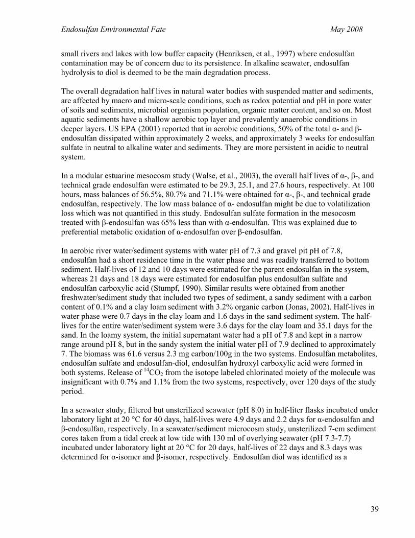
Endosulfan Environmental Fate May 2008
39
small rivers and lakes with low buffer capacity (Henriksen, et al., 1997) where endosulfan contamination may be of concern due to its persistence. In alkaline seawater, endosulfan hydrolysis to diol is deemed to be the main degradation process. The overall degradation half lives in natural water bodies with suspended matter and sediments, are affected by macro and micro-scale conditions, such as redox potential and pH in pore water of soils and sediments, microbial organism population, organic matter content, and so on. Most aquatic sediments have a shallow aerobic top layer and prevalently anaerobic conditions in deeper layers. US EPA (2001) reported that in aerobic conditions, 50% of the total α- and β-endosulfan dissipated within approximately 2 weeks, and approximately 3 weeks for endosulfan sulfate in neutral to alkaline water and sediments. They are more persistent in acidic to neutral system. In a modular estuarine mesocosm study (Walse, et al., 2003), the overall half lives of α-, β-, and technical grade endosulfan were estimated to be 29.3, 25.1, and 27.6 hours, respectively. At 100 hours, mass balances of 56.5%, 80.7% and 71.1% were obtained for α-, β-, and technical grade endosulfan, respectively. The low mass balance of α- endosulfan might be due to volatilization loss which was not quantified in this study. Endosulfan sulfate formation in the mesocosm treated with β-endosulfan was 65% less than with α-endosulfan. This was explained due to preferential metabolic oxidation of α-endosulfan over β-endosulfan. In aerobic river water/sediment systems with water pH of 7.3 and gravel pit pH of 7.8, endosulfan had a short residence time in the water phase and was readily transferred to bottom sediment. Half-lives of 12 and 10 days were estimated for the parent endosulfan in the system, whereas 21 days and 18 days were estimated for endosulfan plus endosulfan sulfate and endosulfan carboxylic acid (Stumpf, 1990). Similar results were obtained from another freshwater/sediment study that included two types of sediment, a sandy sediment with a carbon content of 0.1% and a clay loam sediment with 3.2% organic carbon (Jonas, 2002). Half-lives in water phase were 0.7 days in the clay loam and 1.6 days in the sand sediment system. The half-lives for the entire water/sediment system were 3.6 days for the clay loam and 35.1 days for the sand. In the loamy system, the initial supernatant water had a pH of 7.8 and kept in a narrow range around pH 8, but in the sandy system the initial water pH of 7.9 declined to approximately 7. The biomass was 61.6 versus 2.3 mg carbon/100g in the two systems. Endosulfan metabolites, endosulfan sulfate and endosulfan-diol, endosulfan hydroxyl carboxylic acid were formed in both systems. Release of 14CO2 from the isotope labeled chlorinated moiety of the molecule was insignificant with 0.7% and 1.1% from the two systems, respectively, over 120 days of the study period. In a seawater study, filtered but unsterilized seawater (pH 8.0) in half-liter flasks incubated under laboratory light at 20 °C for 40 days, half-lives were 4.9 days and 2.2 days for α-endosulfan and β-endosulfan, respectively. In a seawater/sediment microcosm study, unsterilized 7-cm sediment cores taken from a tidal creek at low tide with 130 ml of overlying seawater (pH 7.3-7.7) incubated under laboratory light at 20 °C for 20 days, half-lives of 22 days and 8.3 days was determined for α-isomer and β-isomer, respectively. Endosulfan diol was identified as a

Endosulfan Environmental Fate May 2008
40
degradation product (Cotham and Bidleman, 1989). The longer half-lives in seawater/sediment system than those in seawater indicated an endosulfan adsorption onto sediments to compete with degradation.
Water concentrations in California Surface water
California surface water monitoring data was queried from DPR’s surface water monitoring inventory database (DPR, 2007c). The water samples were collected statewide by multiple state and local agencies and other organizations. From 1990 to the end of May 2007, a total of 816 samples for α-endosulfan, 816 samples for β-endosulfan, and 1387samples for endosulfan sulfate were analyzed. Samples were mainly collected in the years from 1991 to 1995 for all three endosulfan forms, and from 2001 to 2004 for endosulfan sulfate only. Endosulfan was found in less than 10% of samples. α-endosulfan in 41 (5.0%), β-endosulfan in 41 (5.0%), and endosulfan sulfate in 127 (9.2%) samples were above the method detection limits (MDLs). The MDLs ranged from 0.00005 to 0.1 µg/L for all three analytes. The lowest concentration detected for all three analytes was 0.005 µg/L; and the highest concentrations were 0.220, 0.039, and 0.628 µg/L for α-, β-endosulfan, and endosulfan sulfate, respectively (Table 17). The detections for α- and β-endosulfan occurred in three counties, Imperial, Sacramento, and Stanislaus, while endosulfan sulfate was detected in four more counties, Los Angeles, Merced, San Joaquin, and Ventura (Table 18). However, except for Imperial County, none of them were listed in Table 4, which listed the counties with mean annual endosulfan use that exceeded 1,000 pounds for the years 1996 to 2005. Although there were no data for the Colorado River itself, endosulfan detections in the Colorado River Basin were reported in the early 1990s. All 36 detections were in the Alamo River in Imperial county and concentration ranged from 0.008 to 0.22 µg/L. In addition, along a transect from the Central Valley to Sequoia National Park, water samples collected from eight sites in 1997 contained α-endosulfan and β-endosulfan ranging from 0.9 – 24.8 ng/L and 0.41 – 140.5 ng/L, respectively (LeNoir et al., 1999). Water samples collected from two lakes in the Sierra Nevada Mountains in 1997 contained endosulfan with concentrations from 0.3 to 1.0 ng/L of α-endosulfan, from 0.17 to 1.8 ng/L of β-endosulfan, and from 0.33 to 2.9 ng/L of endosulfan sulfate (Fellers et al., 2004). Endosulfan was also detected in Lake Tahoe and concentrations ranged from <0.004 to 0.26 ng/L at different depths (McConnell, et al., 1998). Endosulfan residues were also detected in sediment (Gonzalez et al., 1987; Fleck et al., 1991; Ganapathy et al., 1997; Weston et al., 2004) and aquatic organisms, such as mussels (Singhasemanon, 1996), amphibians (Sparling et al., 2001), fish (Singhasemanon, 1995; Brodberg and Pollock, 1999), and frog tissues (Fellers, et al., 2004) and concentrations varied.
Endosulfan Environmental Fate May 2008
41
Table 17. Summary of surface water monitoring results for endosulfan in each year* α-Endosulfan β- Endosulfan Endosulfan sulfate
Samples Detects Concentrations Samples Detects Concentrations Samples Detects Concentrations Year number Number μg/L number number μg/L number number μg/L
1990 0 0 NA 0 0 NA 9 0 NA 1991 220 2 0.012 to 0.022 220 3 0.005 to 0.045 273 43 0.005 to 0.20 1992 229 2 0.005 to 0.008 229 2 0.006 to 0.008 213 18 0.010 to 0.10 1993 125 31 0.008 to 0.220 125 32 0.005 to 0.170 125 48 0.020 to 0.580 1994 134 5 0.016 to 0.068 134 4 0.024 to 0.039 134 5 0.023 to 0.628 1995 105 0 NA 105 0 NA 108 0 NA 1996 3 1 0.002 3 0 NA 3 1 0.12 2001 0 0 NA 0 0 NA 15 6 0.002 to 0.005 2002 0 0 NA 0 0 NA 221 0 NA 2003 0 0 NA 0 0 NA 258 5 0.002 to 0.005 2004 0 0 NA 0 0 NA 28 1 0.002 Total 816 41 816 41 1387 127
*Data was queried from California Department of Pesticide Regulation Surface Water Database (DPR 2007c).
Table 18. Summary of surface water monitoring results for endosulfan in each county with positive detections*
Samples analyzed Endosulfan Detections Highest Concentrations α- β- sulfate- α- β- sulfate- α- β- sulfate- α- β- sulfate- County
number number % μg/L Imperial 65 65 132 36 36 59 55 55 45 0.22 0.17 0.58 Los Angeles 127 9 7 0.022 Merced 190 1 0.5 0.12 Sacramento 188 188 62 1 2 0.5 3 0.002 0.05 San Joaquin 17 2 12 0.2 Stanislaus 238 238 285 4 5 50 1.7 2.1 18 0.22 0.045 0.18 Ventura 7 4 57 0.005 Total 41 41 127 *Data was queried from California Department of Pesticide Regulation Surface Water Database (DPR 2007c).

Endosulfan Environmental Fate May 2008
42
Ground water The Pesticide Contamination Prevention Act requires DPR to maintain a statewide database of wells sampled for pesticide, and state and local agencies to submit results of well sampling for active ingredients to DPR (Nordmark, et al., 2006). Troiano et al. (2001) described the well water monitoring program in details, including criteria for selection of wells, sampling methods, and analytical methods. Well monitoring data is summarized in Table 19. The samples were collected and analyzed by multiple agencies and organizations including DPR (Nordmark, et al., 2006). From 1984 to 2005, total of 4,320, 111, and 3,647 well water samples were analyzed and detected in 12, 0, and 3 samples for α-endosulfan, β-endosulfan, and endosulfan sulfate, respectively. Concentrations ranged from 0.01 – 34.7 μg/L for α-endosulfan and 0.15-0.48 μg/L for endosulfan sulfate with detection limits ranging 0.01-0.05 μg/L for α-endosulfan and 0.1-0.2 μg/L for endosulfan sulfate. However, all 15 detections were classified as “unverified,” because they were not detected in follow-up samples. None detection was ever for β-endosulfan.
Table 19. Summary of endosulfan well water monitoring results (1984-2005)*
α- Endosulfan Endosulfan Sulfate Samples Detections concentration samples detections ConcentrationYear number number ppb number number ppb
1984 339 3 0.02-4.5 219 1985 661 1 0.2 565 1986 401 1 0.01 218 1987 421 256 1988 198 114 1989 86 89 1990 44 44 1991 13 13 1992 34 5 0.05-34.7 35 2 0.22-0.48 1993 66 60 1994 187 2 0.45 186 1995 203 201 1 0.15 1996 19 18 1997 0 0 1998 10 10 1999 22 24 2000 24 24 2001 5 4 2002 143 147 2003 957 956 2004 117 117 2005 296 294 NS** 74 53 Total 4320 12 3647 3
*Data was queried from the DPR’s Well Inventory Database (DPR, 2007d) **Year was not specified in the database.

Endosulfan Environmental Fate May 2008
43
Regional and remote transportation Endosulfan can travel long distances and has been detected all over the world, even in the Arctic. Long range or medium range regional transportation usually involves multiple processes and routes occurring simultaneously in determining ultimate environment fate of endosulfan. Volatilization, vapor transportation, and runoff transportation are the main routes for endosulfan long range and regional transportations. Pesticide contaminations related to regional transportation from Central Valley, California to the Sierra Nevada mountain range were investigated from 1995 to 1997. Table 20 summarized results of three studies related to this investigation. In summertime, LeNoir, et al. (1999) collected samples of air and dry particulate deposition from three locations at elevation of 200, 533, and 1,920 meters, respectively. Duplicated 1-day surface water transect samples were collected from the Central Valley through Sequoia National Park at six elevations from 118 to 2,042 meters. Additional surface water samples were collected from an elevation of 3,231 meters in the Kings Canyon National Park, and 3,322 meters within the Sequoia National Park. In wintertime, McConnell, et al. (1998) collected samples of precipitation, rain and snow, from three locations at elevations of 533, 1,920, and 2,200 meters, respectively. Lake Tahoe water samples were collected from the surface to a depth of 150 meters at the north site, and to a depth of 350 meters at the south sites. In addition, Fellers, et al., 2004, collected water and tissue samples of yellow-legged frog at two locations. Among all samples collected in the three studies, the highest endosulfan concentration (sum of α-, β-, and sulfate endosulfan, if any) was 3.9 ng/m3 for air, 3.6 ng/m2 /day for dry particulate deposit, 165.3 ng/L for water, 7.9 ng/L for rain, 3.5 ng/L for snow, and 1.4 ng/g for frog tissue on a wet weight basis. Endosulfan, predominantly α-endosulfan was found in all air samples and three of the seven dry particulate deposition samples had detectable concentrations of endosulfan. These samples were collected in May to September, 1996, which corresponded with the peak endosulfan use months in the Central Valley, California (Table 5). Three out of the top five endosulfan use counties (Table 4), Fresno, Kings, and Tulare, are in the Central Valley. The Central Valley is an intensive agricultural area lying upwind of the west foot of the Sierra Nevada mountain range. During summer months, delta breezes and prevailing winds can transport endosulfan eastward to the mountain range and deposit as dry particulate on water bodies and ground surfaces. Even at elevations higher than 1,900 meters, endosulfan has been detected in air, particulate, and water samples. In wintertime, endosulfan use was minimum (Table 5) even in the top six use counties (Figure 5), but spraying of dormant orchards in the Central Valley may result in endosulfan in the air, fog, and rain droplet which can be, in turn, be transported to and precipitate, as wintertime rain and snow, in the Sierra Nevada mountain range. In addition, endosulfan transported in summertime may redistribute within the ecosystem of the Sierra Nevada mountain range based on its moderate volatility, adsorption and persistence properties. Endosulfan concentrations in the Lake Tahoe basin water (Fellers, et al., 2004) and snow (McConnell, et al., 1998) samples were generally lower than those from Sequoia National Park which may be explained by the shorter distance from the Central Valley to the Sequoia National Park (McConnell, et al., 1998).

Endosulfan Environmental Fate May 2008
44
Table 20. Summary of monitoring results from three studies in Sierra Nevada Mountains
Samples The highest concentrations Location Number
Detections Endosulfan Type # # # % Unit α- β- sulfate Total*
Summertime sampling in 1996-1997 (LeNoir, et al. 1999) Air 3 12 12 100 ng/m3 3.7 0.6 0.07 3.9 Particulate 3 7 3 43 ng/m2 /day 0.7 3.6 ** 3.6 Surface water 8 8 x2*** 8 100 ng/L 24.8 140.5 ** 165.3
Wintertime sampling in 1995 – 1996 (McConnell, et al., 1998)
Rain 1 7 ** ng/L 6.5 1.4 ** Snow 2 8 ** ng/L 3.0 0.5 ** Tahoe water 2 x4 depths 8 ** ng/L 0.3 **
7.9 3.5 0.3
Amphibian tissue sampling in 1997 (Fellers, et al., 2004)
Surface water 2 4 4 100 ng/L 1.0 1.8 2.9 4.1 Frog tissue 2 40 32 80 ng/g wet wt 1.4 ** ** 1.4
*Sum of the reported α-, β-, and sulfate endosulfan for an individual sample. **No specified data available. ***Duplicate samples were collected at each of 8 locations and the average of the two was reported for each location

Endosulfan Environmental Fate May 2008
45
A similar investigation was conducted in 1986-1988 to look at spray drift and rain runoff from an endosulfan application to a state ecological reserve area, Moss Landing Drainage in Monterey County, California. Following an endosulfan application, CDFA staff collected water, runoff, soil, and sediment samples at the Moss Landing drainage area and in agricultural areas of the Salinas and Carmel River Valleys to evaluate endosulfan distribution (Gonzalez, et al. 1987; Fleck, et al., 1988). For samples collected from Moss Landing Drainage in 1996, endosulfan was detected in 58% of soil and 52% of sediment samples. On a dry weight basis, the highest concentrations of α-, β-, and sulfate endosulfan were 310, 960, 160 µg/kg in soil, respectively, and 52, 1300, and 160 µg/kg in sediment, respectively. The results of the samples from the agricultural area did not support an even distribution for endosulfan. Only 8%, 9%, and 27% of the samples had detectable concentrations of α-, β-, and sulfate endosulfan, respectively (Fleck, et al., 1988). Sediment samples collected from Moss Landing Drainage indicated also an uneven distribution of endosulfan (Gonzalez, et al. 1987). In a spray drift and rain runoff study (Fleck, et al., 1991), deposition, soil, and water samples were collected. An average between 0.005 and 0.019 kg/ha was reported on deposition samples 5.5 meters from the borders of the application field. In addition, rain runoff samples ranged from 2.2 to 13 µg/L indicating another route of off-site movement of the applied endosulfan. The average of soil endosulfan was 1,548 and 2,962 µg/kg for pre- and post-application. These results were comparable with other study in this region. In Europe, atmospheric deposition of endosulfan on mountain lakes in the Alps, Pyrenees, and Caledonian Mountains was estimated between 0.2 – 340 ng /m2
-month (Carrera, 2002). The southern lakes contained higher concentrations, reflecting the agricultural activities in southern Europe. In the northern lake only the more recalcitrant endosulfan sulfate was detected. Studies have shown that endosulfan has even been transported to the Arctic. It has been detected in both east (Russia) and west (Canada) sides in atmospheric air, rain, snow, ice and fine particulate, water ways of lake, river, and sea, sediment, soil, plants, and amphibians, etc (Gregor and Gumme, 1989; Barrie, et al., 1992; Blais, et al., 1998, Konoplev, et al., 2002; De Wit, et al., 2002; Chernyak, et al., 1996). Mean water concentrations ranged from 2-10 pg/L (INAC, 2002). Seasonal trends showed increasing concentrations during the open water season suggesting fresh input from gas exchange and runoff. This trend parallels seasonal trends observed in Arctic air. The spatial distribution of organochlorine pesticides spanned the Arctic Ocean from the Bering and Chukchi seas to the North Pole, to a station north of Spitsbergen, and then south into the Greenland Sea. Spatial differences in concentration varied with the observed pesticide. A reverse trend was found for endosulfan, with lower concentrations in the ice-covered regions (Jantunen and Bidleman, 1998). Briggs, et al. (1998) monitored endosulfan concentrations in rivers and daily rainfall observations from 23 stations in a cotton production region for five years. On plotting α- and β-endosulfan fractions of each observed peak concentration versus antecedent rainfall events, it was found that endosulfan concentration peaks fell mainly into two distinct regions: (a) events with little antecedent rainfall and high fractions of α- and β-endosulfan primarily by airborne transport, and (b) events with high antecedent rainfall and low fractions of α- and β- endosulfan primarily by waterborne transport. Some events occurred in a third region (c) with low antecedent rainfall and low fractions of α- and β-endosulfan, but arising from the continued

Endosulfan Environmental Fate May 2008
46
presence of endosulfan sulfate with a long riverine residence time. Very few events are observed in the fourth region with high antecedent rainfall and high fractions of α- and β- endosulfan. Events in regions (a) and (b) were both of significant magnitude, with (a) being dominant at locations close to cotton farms. The data analysis indicated that airborne transport accounted for a significant fraction, around 50%, of the endosulfan concentrations in slow-flowing waterways close to cotton farms. Waterborne transport could only occur after rainfall. Dust transport and subsurface leaching were of negligible magnitude for endosulfan regional transport. Fate and persistence in biota Endosulfan is not persistent in biota and not susceptible to bioaccumulation. Therefore, it is not hazardous if applied at recommended rates and following the label instructions. For terrestrial animals and most aquatic organisms, it is metabolized very fast to a low plateau level of residues. On the other hand, endosulfan is highly toxic to some aquatic species, particularly fish. Fish are extremely sensitive to endosulfan. Fish kills due to discharge of endosulfan into rivers have been reported. Application of endosulfan to wetlands at recommended rates may well result in killing of fish. Half lives of α-, β-, and α- + β-endosulfan were estimated of 2.01±0.44, 1.74±0.33, 1.81±0.35 days, respectively for the fish species Yellow Tetra (Hyphessobrycon bifasciatus) (Jonsson and Toledo, 1993). An anti-oxidant, selenium, was claimed to reverse the toxic implication of endosulfan in fish (Shafiq-ur-Rehman, 2006). Endosulfan is moderately toxic for honey bees. Toxicity for birds is high in a laboratory setting, but no poisonings have been reported under field conditions.

Endosulfan Environmental Fate May 2008
47
Reference Ahmad, N., V. Edge, and P. Rohas. 1995. Aerial Transport of Endosulfan. Proc. Annual Program
Workshop, Minimizing the Impact of Pesticides on the Riverine Environment, Sydney, 22-23 August 1995. Land and Water Resources Research and Development Corporation.
Al-Hassan, R.M., I.I. Bashour, N.S. Kawar. 2004. Biodegradation of alpha and beta endosulfan
in soil as influenced by application of different organic materials. J Environ Sci Health B. 39(5-6), 757 – 764.
ARB. 1998. Report for the air monitoring of endosulfan in Fresno County (ambient) and in San
Joaquin County (application). California Air Resources Board, California Environmental Protection Agency (CalEPA). Sacramento, California.
Atkinson, R. 1987. A structure-activity relationship for the estimation of rate constants for the
gas-phase reactions of OH radicals with organic compounds. International Journal of Chemical Kinetics. Vol. 19, 799-828.
Awasthi, N., N. Manickam, and A. Kumar. 1997. Biodegradation of endosulfan by a bacterial co
culture. Bull. Environ. Contam. Toxicol. 59:928–934. Barrie, L.A., D. Gregor, B. Hargrave, R. Lake, D. Muir, R. Shearer, B. Tracey, and T. Bidleman.
1992. Arctic contaminants: sources, occurrence and pathways. Sci. Tot. Environ. 122, 1-74.
Beil, S., Kertesz, M.A., Leisinger, T. and Cook, A.M. (1996) The assimilation of sulfur from
multiple sources and its correlation with expression of the sulfate-starvation-induced stimulon in Pseudomonas putida S-313. Microbiology 142, 1989–1995.
Blais, J.M., D.W. Schindler, D.C.G. Muir, L.E. Kimpe, D.B. Donals, and B. Rosenberg. 1998.
Accumulation of Persistent Organochlorine Compounds in mountains of Western Canada. Nature. 395 (8), 585-588.
Briggs, R.P., M.R. Raupach, B. Cooper, and M. Muschal. 1998. Integrative modelling of
transport and fate of endosulfan in the riverine environment. Part I: Use of observed riverine concentrations to identify contributions of airborne and waterborne transport. CSIRO Land and Water Technical Report 14/98. http://www.clw.csiro.au/publications/technical98/tr14-98.pdf
Brodberg, R.K. and G.A. Pollock. 1999. Prevalence of Selected Target Chemical Contaminants
In Sport Fish from Two California Lakes, Public Health Designed Screening Study. Office of Environmental Health Hazard Assessment, CalEPA. Sacramento, CA.
Carrera G., P. Fernandez, J.O. Grimalt, M. Ventura, L. Camarero, J. Catalan, U. Nickus, H.
Thies, and R. Psenner. 2002. Atmospheric deposition of organochlorine compounds to remote high mountain lakes of Europe. Environ. Sc. Technol. 36(12), 2581-2588.

Endosulfan Environmental Fate May 2008
48
Chernyak, S.M., C.P. Rice, and L.L. McConnell. 1996. Evidence of currently-used pesticides in
air, ice, fog, seawater and surface microlayer in the Bering and Chukchi Seas. Marine Pollution Bulletin 22 (5), 410-419.
Cotham, E.W. Jr. and T.F. Bidleman. 1989. Degradation of Malathion, Endosulfan, and
Fenvalerate in Seawater and Seawater/Sediment Systems. J. Agric. Food Chem. 37, p. 824-828.
De Wit, C.A., A.T. Fisk, K.E. Hobbs, and D.C.G. Muir. 2002. Levels, trends and effects of
Persistent Organic Pollutants (POPs) in the Arctic environment. 2nd AMAP International Symposium on Environmental Pollution in the Arctic, Rovaniemi 1-3 October 2002.
DPR. 1996. Use Information and Air Monitoring Recommendation for the Pesticidal Active
Ingredient Endosulfan. Environmental Monitoring Branch, Department of Pesticide Regulation, CalEPA. Sacramento, California.
DPR. 2004. Summary of Physical and Chemical Properties. Pesticides Database. Environmental
Monitoring Branch, Department of Pesticide Regulation, CalEPA. Sacramento, California. http://dpr01.inside.cdpr.ca.gov:8000/cgi-bin/cheminfo/cheminfo.pl
DPR. 2007a. Registration status. Product/Label Database. Department of Pesticide Regulation,
CalEPA. Sacramento, California. DPR. 2007b. Pesticide use database. Department of Pesticide Regulation, CalEPA. Sacramento,
California. DPR 2007c. California Department of Pesticide Regulation Surface Water Database. Accessed
on June 1, 2007 by Keith Starner. Department of Pesticide Regulation, CalEPA. Sacramento, California.
DPR 2007d. California Department of Pesticide Regulation Well Water Database. Accessed on
May 30, 2007 by Craig Nordmark. Department of Pesticide Regulation, CalEPA. Sacramento, California.
El Zorganir, G. A., and M. E. H. Omer. 1974. Metabolism of endosulfan isomers by Aspergillus
niger. Bull. Environ. Contam. Toxicol. 12:182–185. EXTOXNET. 2007. Pesticide Information Profiles-Endosulfan. Extension Toxicology Network. http://extoxnet.orst.edu/pips/reflist6.htm Fellers, M.G., L. L. McConnell, D. Pratt, and S. Datta. 2004. Pesticides in Mountain Yellow-
Legged Frogs (Rana Muscosa) from the Sierra Nevada Mountains of California, USA. Environmental Toxicology and Chemistry, Vol. 23, No. 9, pp. 2170–2177.

Endosulfan Environmental Fate May 2008
49
Fleck, J., L. J. Ross, and K. Hefner. 1988. Endosulfan and Chlorthal-Dimethyl Residues in Soil and Sediment of Monterey County. Report No. EH 88-6. Environmental Monitoring Branch. Department of Pesticide Regulation, CalEPA. Sacramento, CA.
Fleck, J., L. J. Ross, D. Tran, J. Melvin, and B. Fong. 1991. Movement of endosulfan from
artichoke fields in Monterey County. Report No. EH 91-05. Environmental Monitoring Branch. Department of Pesticide Regulation, CalEPA. Sacramento, CA. http://www.cdpr.ca.gov/docs/empm/pubs/ehapreps/eh9105.pdf.
FOOTPRINT. 2007. FOOTPRINT Pesticide Properties Database. University of Hertfordshire &
FOOTPRINT. http://www.herts.ac.uk/aeru/footprint/en/ Galarneau, E., C.V. Audette, A. Bandemehr, I. Basu, T.F. Bidleman, K.A. Brice, D.A. Burniston,
C.H. Chan, F. Froude, R.A. Hites, M.L. Hulting, M. Neilson, D. Orr, M.F. Simcik, W.M.J. Strachan, and R.M. Hoff. 2000. Atmospheric Deposition of Toxic Substances to the Great Lakes. IADN Results to 1996, IADN (Integrated Atmospheric Deposition Network), published by Environment Canada and US EPA (2000).
Ganapathy, C., C. Nordmark, K. Bennett, A. Bradley, H. Feng, J. Hernandez, and J. White. 1997.
Temporal Distribution of Insecticide Residues in Four California Rivers. Report No. EH 97-06. Environmental Monitoring Branch, Department of Pesticide Regulation, CalEPA. Sacramento, Ca. http://www.cdpr.ca.gov/docs/empm/pubs/ehapreps/eh976rep.pdf.
GFEA (German Federal Environment Agency). 2004. Draft Dossier prepared in support of a
proposal of endosulfan to be considered as a candidate for inclusion in the UN-ECE LRTAP protocol on persistent organic pollutants. German Federal Environment Agency. Umweltbundesamt, Berlin. http://www.unece.org/env/popsxg/docs/2004/Dossier_Endosulfan.2004.pdf
Goel, A., L.L. Mcconnell, and A. Torrents. 2005. Modeling the variability in aerial concentration
of atrazine, endosulfan and chlorothalonil at a rural location on the delmarva peninsula [abstract]. American Chemical Society 230th National Meeting. Paper No. 71, P. 67.
Goerlitz, G. and U. Eyrich. 1987a. Endosulfan adsorption/desorption on the system soil/water.
Part I: alpha-endosulfan, beta-endosulfan. AgrEvo Doc. A37591, unpublished report. Goerlitz, G. and U. Eyrich. 1987b. Endosulfan adsorption/desorption on the system soil/water.
Part II: Metabolites Endosulfan-sulfate, Endosulfan-diol AgrEvo Doc. A39353, unpublished report.
Gonzalez, D., L.J. Ross, R. Segawa, and B. Fong. 1987. Variation of Endosulfan Residues in
Water and Sediment Taken from the Moss Landing Drainage of Monterey County. Report EH 87-02. Environmental Monitoring Branch, Department of Pesticide Regulation, CalEPA. Sacramento, CA. http://www.cdpr.ca.gov/docs/empm/pubs/ehapreps/eh8702.pdf.

Endosulfan Environmental Fate May 2008
50
Gregor, D.J. and W. Gumme.1989. Evidence of atmospheric transport and deposition of
organochlorine pesticides and PCB in Canadian Arctic snow. Environ. Sci. Technol. 23 (5), 561-565.
Greve, P.A. and S.L. Wit. 1971. Endosulfan in the Rhine river. Journal of the Water Pollution
Control Federation 43, 2338-2348. Guerin, T. F. 1999. The anaerobic degradation of endosulfan by indigenous microorganisms
from low-oxygen soils and sediments. Environ. Pollut. 106:13–21. Guerin, T.F. 2001. Abiological loss of endosulfan and related chlorinated organic compounds
from aqueous systems in the presence and absence of oxygen. Environmental Pollution 115, p.219-230.
Halsall, C.J., R. Bailey, G.A. Stern, L.A. Barrie, P. Fellin, D.C.G. Muir, B. Rosenberg, F.Y.
Rovinsky, E.Y. Kononov, and B. Pastukhov. 1998. Multi-year observations of organohalogen pesticides in the Arctic atmosphere. Environmental Pollution 102, 51-62.
Hayes, S.P. and P.T. Phillips. 1984. California State Mussel Watch Marine Water Quality
Monitoring Program 1983-1984. Water Quality Monitoring Report No. 85-2 WQ. California State Water Resources Control Board and Department of Fish and Game. Sacramento, Ca.
Hengpraprom, S. and C. Lee. 1998. Case Study in Environmental Chemistry, Hydrolysis of
endosulfan. Environmental Engineering and Science, Clemson University. http://www.ces.clemson.edu/ecl/caseStudy/case2.pdf
Hengpraprom, S., C. Lee, J. Coates, Alan Elzerman, and Steve Klaine. 2002. The Effect of
Kaolinite and Soil Organic Matter on the Hydrolysis of α-Endosulfan. SETAC 2002. (P886).
Hengpraprom, S. 2004 Hydrolysis of α-Endosulfan in Mineral-Humic Acid Suspensions. SETAC 2004. (PH057).
Henriksen, A., B.L. Skjelkvåle, J. Mannio, A. Wilander, J.P. Jensen, T. Moiseenko, R. Harriman, T.S. Traaen, E. Fjeld, J. Vuorenmaa, P. Kortelainen, and M. Forsius.1997. Results of national lake surveys in 1995 in Finland, Norway, Sweden, Denmark, Russian Kola, Russian Karelia, Scotland and Wales. NIVA Report SNO 3645-97, p.43
Hinck, J. E., V. S. Blazer, N. D. Denslow, T. S. Gross, K. R. Echols, A.P. Davis, T. W. May, C.
E. Orazio, J. J. Coyle, and D. E. Tillitt. 2006. Biomonitoring of Environmental Status and Trends (BEST) Program: Environmental Contaminants, Health Indicators, and Reproductive Biomarkers in Fish from the Colorado River Basin. SIR 2006-5163 Abstract. http://pubs.usgs.gov/sir/2006/5163/sir5163abs.html

Endosulfan Environmental Fate May 2008
51
Hummerjohann, J., Kuttel, E., Quadroni, M., Ragaller, J., Leisinger, T. and Kertesz, M.A. (1998) Regulation of the sulfate starvation response in Pseudomonas aeruginosa: role of cysteine biosynthetic intermediates. Microbiology 144, 1375–1386.
Hung, H., C.J. Halsall, P. Blanchard, H. Li, P. Fellin, G. Stern, and B. Rosenberg. 2002.
Temporal trends of organochlorine pesticides in the Canadian Arctic atmosphere. Environ. Sci. Technol., 36, 862-868.
INAC. 2002. Indian and Northern Affairs Canada. The Canadian Arctic Contaminants
Assessment Report II (CACAR II). Jantunen, L. M. and T. F. Bidleman. 1998. Organochlorine Pesticides and Enantiomers of Chiral
Pesticides in Arctic Ocean Water. Arch. Environ. Contam. Toxicol. 35, 218–228. Jonas, W. 2002. Degradation of 14C Endosulfan in two aerobic water/sediment systems. Aventis
Crop Science study number NA 019404 (2002) Jonsson, M.C. and M.C.F. Toledo. 1993. Bioaccumulation and elimination of endosulfan in the
fish yellow tetra (Hyphessobrycon bifasciatus). Bull. Environ. Contam. Toxicol. (1993) 50:572-577
Kathpal, S. T., A. Singh, J.S. Dhankhar, and G. Singh. 1997. Fate of Endosulfan in Cotton Soil
under Sub-tropical Conditions of Northern India. Pestic. Sci. 50:1, 21-27. Katayama, A and Matsumura, F. 1993. Degradation of organochlorine pesticides, particularly
endosulfan, by Trichoderma harzianum. Environmental Toxicology and Chemistry, v. 12, no. 6, p. 1059-1065.
Kennedy, I. R., F. Sa´nchez-Bayo, S. W. Kimber, L. Hugo, and N. Ahmad. 2001. Off-Site
Movement of Endosulfan from Irrigated Cotton in New South Wales. J. Environ. Qual. 30: 683–696.
Kertesz, M.A., Leisinger, T. and Cook, A.M. (1993) Proteins induced by sulfate limitation in
Escherichia coli, Pseudomonas putida, or Staphlococcus aureus. Journal of Bacteriology 175, 1187–1190.
Kim, Y. K., S. H. Kim and S. C. Choi. 2001. Kinetics of endosulfan degradation by
Phanerochaete chrysosporium. Biotechnology Letters, 23: 163-166. Klöpffer, W. and E. G. Kohl. 1993. Bomolecular OH rate constants of organic compounds in
solution. 2. measurements in 1,2,2-trichlorotrifluoroethane using hydrogen peroxide as an OH source. Ecotoxicology & Environmental Safety, 26, 346-356.
Konoplev, A., P. Fellin, H. Li, P. Blanchrd, H. Hung, D. Samsonov, and G. Stern. 2002.
Monitoring of POPs in Arctic ambient air: Initial results from Anderma (Russia) and

Endosulfan Environmental Fate May 2008
52
preliminary assessment. 2nd AMAP International Symposium on Environmental Pollution in the Arctic, Rovaniemi 1-3 October 2002
Krol, M., van Leauwen, P.J., and Lelieveld, J., 1998. Global OH trend inferred from
methylchloroform measurements. Journal of Geophysical Research-Atmospheres 103, 10697–10711.
Kullman, S. W AND Fumio Matsumura. 1996. Metabolic Pathways Utilized by Phanerochaete
chrysosporium for Degradation of the Cyclodiene Pesticide Endosulfan. Applied and Environmental Microbiology, Vol. 62, No. 2, p. 593-600.
LeNoir, J.S., L.L. McConnell, G.M. Fellers, T.H. Cahill, and J.N. Seiber. 1999. Summertime
transport of current-use pesticides from California’s Central Valley to the Sierra Nevada mountain range. Environmental Toxicology and Chemistry. 18:2715-2722.
Leys, J.F., F.J. Larney, J.F. Müller, M.R. Raupach, M.R. McTainsh, and G.H. Lynch. 1998.
Anthropogenic dust and endosulfan emissions on cotton farm in northern New South Wales, Australia. Sci. Tot. Environ. 220, 55-70 (1998).
Lyman, W.J., W.F. Rechl, and D.H. Rosenblaff. 1990. Handbook of Chemical Property
Estimation Methods. ACS. Martens Rainer. 1976. Degradation of [8,9-14C]Endosulfan by Soil Microorganisms. Applied
and Environmental Microbiology, vol. 31, no. 6, p. 853-858. McCall, E.C., Jr., G.I. Scott, and J.M. Hurley. 1988. A comparison of agricultural nonpoint
source runoff from black plastic and conventional-till tomato test plots. South Carolina Water Resour. Res. Inst. Tech. Completion Rep. G1251-07. Rep. no. 126. Clemson Univ., Clemson, SC.
McConnell, L.L., J.S. Lenoir, S. Datta, and J.N. Seiber. 1998. Wet deposition of current-use
pesticides in the Sierra Nevada mountain range, California. Environ. Toxicol. Chem. 17(10), 1908-1916.
Miles, J.R.W. and P. Moy. 1979. Degradation of endosulfan and its metabolites by a mixed
culture of soil microorganisms. Bull. Environ. Contam. Toxicol., 23, 13-19. Mukherjee, I., and M. Gopal. 1994. Degradation of beta-endosulfan by Aspergillus niger.
Toxicol. Environ. Chem. 46:217–221. Nordmark, C., J. Dias, M. Clayton, J. Troiano, and M. Pepple. 2006. Update of the Well
Inventory Database. Report No. EH 06-05. Environmental Monitoring Branch. Department of Pesticide Regulation, California Environmental Protection Agency. Sacramento, CA. http://www.cdpr.ca.gov/docs/empm/pubs/ehapreps/eh0605.pdf

Endosulfan Environmental Fate May 2008
53
Okumura, D.Y. 1991. Suggested Criteria for Issuance of Endosulfan Permits and Suggested Permit Conditions. Letter No. ENF 91-12 to County Agricultural Commissioners from Douglas Y. Okumura, Chief, Pesticide Enforcement Branch, DPR, dated January 29. Department of Pesticide Regulation, CalEPA. Sacramento, CA.
Okumura, D.Y. 1992. Development of Endosulfan Regulations. Letter No. ENF 92-10 to County
Agricultural Commissioners from Douglas Y. Okumura, Chief, Pesticide Enforcement Branch, DPR, dated January 31. Department of Pesticide Regulation, CalEPA. Sacramento, CA.
Palm, W.U. and C. Zetzsch. 1991. Estimation of the rate constants for the reaction of alpha- and
beta-endosulfan with OH radicals by the incremental procedure of Atkinson. AgrEvo Doc. No. A48681, unpublished results.
PANNA. 2007. Air Monitoring in Hastings, Florida December 6–14, 2006: Technical Report.
page 10. Pesticide Action Network North America. San Francisco, CA. Patton, G.W., D.A. Hinckley, M.D. Walla, and T.F. Bidleman. 1989. Airborne organochlorines
in the Canadian High Arctic. Tellus, 41B, 243-255 (1989). Peterson, S.M. and Batley, G.E. 1993. The fate of endosulfan in aquatic ecosystems.
Environmental Pollution 82:143-152. Rao, D. M. R., and A. S. Murty. 1980. Persistence of endosulfan in soils. J. Agric. Food Chem.
28:1099–1101. Raupach, M. R., P. R. Briggs, P. W. Ford, J. F. Leys, M. Muschal, B. Cooper, and V. E. Edge.
2001. Endosulfan Transport: I. Integrative Assessment of Airborne and Waterborne Pathways. J. Environ. Qual. 30:714–728.
Rice, C., C. Nochetto, and P. Zara. 2002. Volatilization of trifluralin, atrazine, metolachlor,
chlorpyrifos, α-endosulfan and β-endosulfan from freshly tilled soil. Journal of Agricultural and Food Chemistry 50:4009-4017.
Rice, C.P., S.M. Chernyak, C.J. Hjapeman, and S. Boilboulian. 1997. Air-water distribution of
the endosulfan isomers. J. Environ. Qual. 26, 1101-1106 (1997). Rice, J. P., L.L. McConnell, L.P. Heighton, A.M. Sadeghi, A.R. Isensee, J.R. Teasdale, A.A.
Abdul-Baki, J.A. Harman-Fetcho, and C.J. Hapeman. 2001. Runoff Loss of Pesticides and Soil: A Comparison between Vegetative Mulch and Plastic Mulch in Vegetable Production Systems. J. Environ. Qual. 30:1808–1821 (2001).
Rüdel H. 1997. Volatilization of pesticides from soil and plant surfaces, Chemosphere 35 (1997)
pp.143–152.

Endosulfan Environmental Fate May 2008
54
Sava, R.J. 1985. Monterey County Residential Air Monitoring. Report No. EH 85-07. Environmental Monitoring Branch, Department of Pesticide Regulation, CalEPA. Sacramento, CA. http://www.cdpr.ca.gov/docs/empm/pubs/ehapreps/eh8507.pdf.
Schmidt, W.F., S. Bilboulian, C.P. Rice, J.C. Fettinger, L.L. McConnell, and C.J. Hapeman.
2001. Thermodynamic, spectroscopic, and computational evidence for the irreversible conversion of β- to α-endosulfan. Journal of Agricultural and Food Chemistry 49:5372-5376.
Schneider, M., and K. Ballschmiter. 1995. Transformation experiments with two chiral
endosulfan metabolites by soil microorganisms—CHIRAL HRGC on lipophilic cylodestrin derivatives. Fresenius’ J. Anal. Chem. 352: 756–762.
Sethunathan, N., M. Megharaj, Z. Chen, N. Singh, R.S. Kookana, and R. Naidu. 2002.
Persistence of endosulfan and endosulfan sulfate in soil as affected by moisture regime and organic matter addition. Bull. Environ. Contam. Toxicol, vol. 68, p. 725-731.
Shafiq-ur-Rehman. 2006. Endosulfan Toxicity and its Reduction by Selenium:
A Behavioral, Hematological and Peroxidative Stress Evaluation. The Internet Journal of Toxicology. 2006. Volume 3, Number 1.
Shetty, P. K., J. Mitra, N. B. K. Murthy, K. K. Namitha, K. N. Savitha and K. Raghu. 2000.
Biodegradation of cyclodiene insecticide endosulfan by Mucor thermohyalospora MTCC 1384. CURRENT SCIENCE, Vol. 79, No. 9.
Siddique, T., B. C. Okeke, M. Arshad, and W. T. Frankenberger, Jr. Enrichment and Isolation of
Endosulfan-Degrading Microorganisms. Environ. Qual. 32:47–54 (2003). Singhasemanon, N. 1995. Review of the Toxic Substances Monitoring Program’s 1993-1994
Preliminary Data Report. Memo dated October 16. Environmental Monitoring Branch, Department of Pesticide Regulation, CalEPA. Sacramento, CA
Singhasemanon, N. 1996. Review of the State Mussel Watch 1995 Survey Preliminary Data
Report. Memo dated August 30. Environmental Monitoring Branch, Department of Pesticide Regulation, CalEPA. Sacramento, CA
Sparling, D.W., G.M. Fellers, and L.L. McConnell. 2001. Pesticides and amphibian population
declines in California, USA. Environmental Toxicology and Chemistry 20:1591-1595. Stephenson, M., S. Coale, M. Martin, and J. Martin. 1980. California State Mussel Watch Marine
Water Quality Monitoring Program 1979-80. Water Quality Monitoring Report No. 80-8. California State Water Resources Control Board, Technical Services Division. Sacramento, CA.
Strachan, R.M.H. 2000. Atmospheric Deposition of Toxic Substances to the Great Lakes. IADN
Results to 1996. IADN (Integrated Atmospheric Deposition Network). published by Environment Canada and US EPA, 2000.

Endosulfan Environmental Fate May 2008
55
Stumpf, K. 1990. Comments regarding the Dutch Hazard Assessment of Endosulfan Concerning
the Bioavailability in Water/Sediment Systems. HOE Doc. A44231, unpublished. Stumpf, K. and C. Schink. 1988. Photodegradation of alpha-Endosulfan (HOE052618) and beta-
Endosulfan (Hoe 052619) in Water. AgrEvo Doc. No. A37588, unpublished results. Sutherland, T.D., I. Horne, M.J. Lacey, R.L. Harcourt, R.J. Russell, and J.G. Oakeshott. 2000.
Enrichment of an Endosulfan-Degrading Mixed Bacterial Culture. Applied and Environmental Microbiology, Vol. 66, No. 7, p. 2822–2828.
Sutherland, T.D., I. Horne, R.L. Harcourt, R.J. Russell and J.G. Oakeshott. 2002a. Isolation and
characterization of a Mycobacterium strain that metabolizes the insecticide endosulfan. Journal of Applied Microbiology, v 93, p. 380–389.
Sutherland, T.D., K.M. Weir, M.J. Lacey, I. Horne, R.J. Russell and J.G. Oakeshott. 2002b.
Enrichment of a microbial culture capable of degrading endosulphate, the toxic metabolite of endosulfan. Journal of Applied Microbiology, 92, 541±548
Sutherland, T.D., I. Horne, R.J. Russell, and J.G. Oakeshott. 2002c. Gene Cloning and Molecular
Characterization of a Two-Enzyme System Catalyzing the Oxidative Detoxification of _ β-Endosulfan. Applied and Environmental Microbiology, Vol. 68, No. 12, p. 6237–6245
Teske, E.M., S. Bird, D. Easterly, S. Ray, and S. Perry. 1997. A user guide for AgDRIFT 1.0: A
tiered approach for the assessment of spray drift of pesticides. CDI Tech. Note no. 95-10. Prepared on behalf of the Spray Drift Task Force, c/o Stewart Agric. Res. Services, Macon, MO.
Tomlin, C.D.S. (editor). 1994. The Pesticide Manual, 10th Edition. British Crop Protection
Council and The Royal Society of Chemistry, United Kingdom. The Bath Press, Bath. Troiano, J., D. Weaver, J. Marade, F. Spurlock, M. Pepple, C. Nordmark, and D. Bartkowiak.
2001. Summary of well water sampling in California to detect pesticide residues resulting from nonpoint-source applications. Journal of Environmental Quality 30:448-459.
US EPA. 2001. Environmental Fate and Ecological Risk Assessment for the Reregistration
Eligibility Decision on Endosulfan. US EPA, Office of Prevention, Pesticides, and Toxic Substances
US EPA. 2002. Endosulfan RED Facts. US EPA, Office of Prevention, Pesticides.
http://www.epa.gov/oppsrrd1/REDs/factsheets/endosulfan_fs.htm US EPA. 2006a. Endosulfan, Fenarimol, Imazalil, Oryzalin, Sodium Acifluorfen, Trifluralin, and
Ziram; Tolerance Actions. Federal Register: September 15 2006, Volume 71, Number 179, Rules and Regulations, Page 54423-54434.
http://www.epa.gov/fedrgstr/EPA-PEST/2006/September/Day-15/p15258.htm

Endosulfan Environmental Fate May 2008
56
US EPA. 2006b. Great Lakes Monitoring. Integrated Atmospheric Deposition Network (IADN), Information Resources. http://www.epa.gov/glnpo/monitoring/air/iadn/iadn.html
Van Woerden, H.F. 1963. Organic sulfites. Chem. Rev. 63: 557-571. Walse, S.S., G.I. Scott, and J.L. Ferry. 2003. Stereoselective degradation of aqueous endosulfan
in modular estuarine mesocosms: formation of endosulfan γ-hydroxycarboxylate. J. Environ. Monit., 2003. 5: 373-379.
Weston, D.P., J. You, and M.J. Lydy. 2004. Distribution and toxicity of sediment associated pesticides in agriculture-dominated water bodies of California's Central Valley. Environmental Science and Technology 38:2752-2759.
WHO. 1988. A companion volume to Environmental Health Criteria 40: Endosulfan. Published
by the WHO for the INTERNATIONAL PROGRAMME ON CHEMICAL SAFETY, Health and Safety Guide No. 17. Geneva, Switzerland. http://www.inchem.org/documents/hsg/hsg/hsg017.htm
Wilhoit, L. 1998. A Computer Program to Identify Outliers in the Pesticide Use Report
Database. Report No. PM 98-01. Pesticide Management Branch, Department of Pesticide Regulation, CalEPA. Sacramento, CA.
Woods, N., I. P. Craig, G. Dorr, and B. Young. 2001. Spray Drift of Pesticides Arising from
Aerial Application in Cotton. J. Environ. Qual. 30:697-701 Zetzsch, C. 1992. Photochemisch-oxidativer Abbau von alpha-Endosulfan in der Gasphase.
AgrEvo Doc. No. A48146, unpublished results. Zhou, M., Y.C. Li, P. Nkedi-Kizza, and S.K. O’Hair. 2003. Endosulfan Losses through Runoff
and Leaching from Calcareous Gravelly or Marl Soils. Vadose Zone Journal, 2:231–238.