energy derivatives optimisation & pricingdelmas/enseig/levy-delatour... · 2016-03-04 ·...
TRANSCRIPT
Energy derivatives – Optimisation & Pricing
February 2015 Arnaud de Latour, [email protected]
Outline
Energy derivatives modelling
A typical energy portolio
Market modelling of some energy derivatives :
Swaps, power plants, storage assets, load-curve contracts, …
Some pricing methods will be detailed for…
Spread options
Swing options
Disclaimer ! Any views or opinions presented in this presentation are solely those of the author and do not necessarily represent those of the EDF group.
1 – Energy derivatives

ENERGY DERIVATIVES
A typical energy portfolio
Forwards, Swaps and Spreads
Power plant modelling, Spread options pricing
Gas storage modelling
Swing options pricing
Load curve contract modelling
2 – Energy derivatives
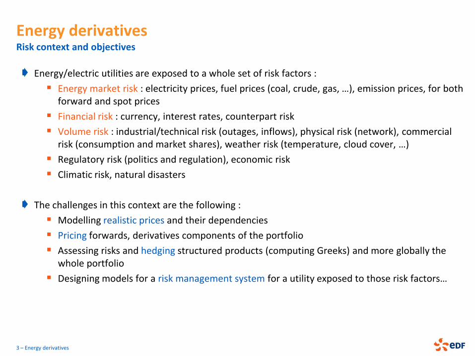
Energy derivatives Risk context and objectives
Energy/electric utilities are exposed to a whole set of risk factors :
Energy market risk : electricity prices, fuel prices (coal, crude, gas, …), emission prices, for both forward and spot prices
Financial risk : currency, interest rates, counterpart risk
Volume risk : industrial/technical risk (outages, inflows), physical risk (network), commercial risk (consumption and market shares), weather risk (temperature, cloud cover, …)
Regulatory risk (politics and regulation), economic risk
Climatic risk, natural disasters
The challenges in this context are the following :
Modelling realistic prices and their dependencies
Pricing forwards, derivatives components of the portfolio
Assessing risks and hedging structured products (computing Greeks) and more globally the whole portfolio
Designing models for a risk management system for a utility exposed to those risk factors…
3 – Energy derivatives
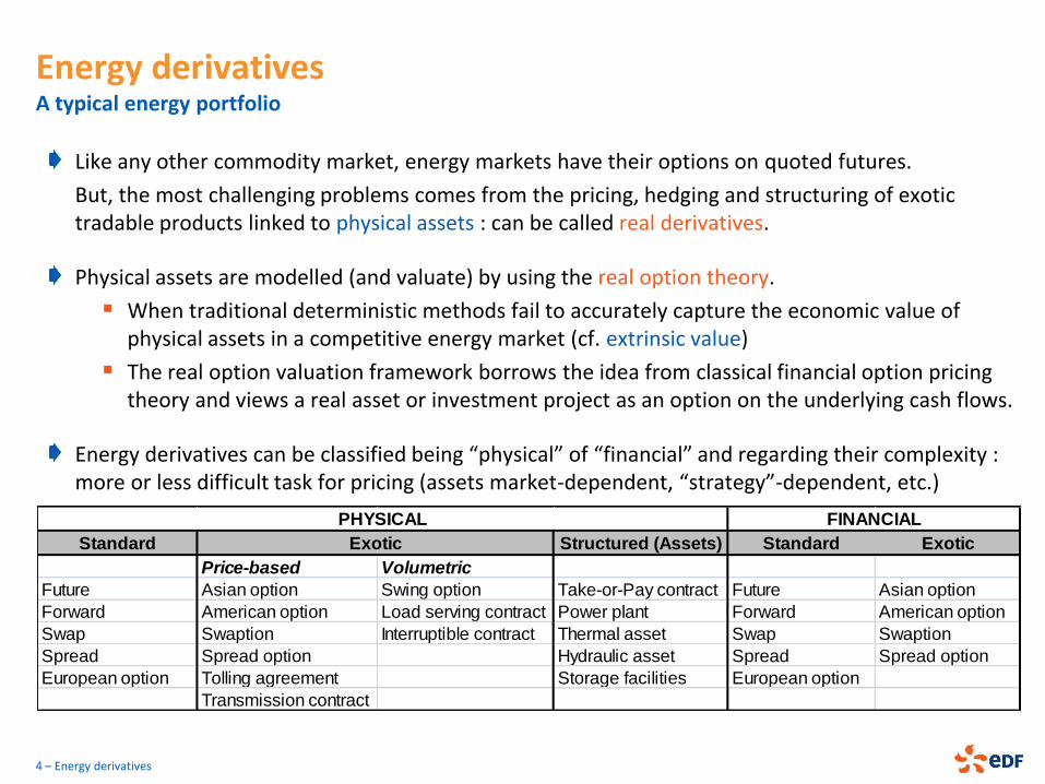
Energy derivatives A typical energy portfolio
Like any other commodity market, energy markets have their options on quoted futures.
But, the most challenging problems comes from the pricing, hedging and structuring of exotic tradable products linked to physical assets : can be called real derivatives.
Physical assets are modelled (and valuate) by using the real option theory.
When traditional deterministic methods fail to accurately capture the economic value of physical assets in a competitive energy market (cf. extrinsic value)
The real option valuation framework borrows the idea from classical financial option pricing theory and views a real asset or investment project as an option on the underlying cash flows.
Energy derivatives can be classified being “physical” of “financial” and regarding their complexity : more or less difficult task for pricing (assets market-dependent, “strategy”-dependent, etc.)
4 – Energy derivatives
Standard Structured (Assets) Standard Exotic
Price-based Volumetric
Future Asian option Swing option Take-or-Pay contract Future Asian option
Forward American option Load serving contract Power plant Forward American option
Swap Swaption Interruptible contract Thermal asset Swap Swaption
Spread Spread option Hydraulic asset Spread Spread option
European option Tolling agreement Storage facilities European option
Transmission contract
PHYSICAL FINANCIAL
Exotic
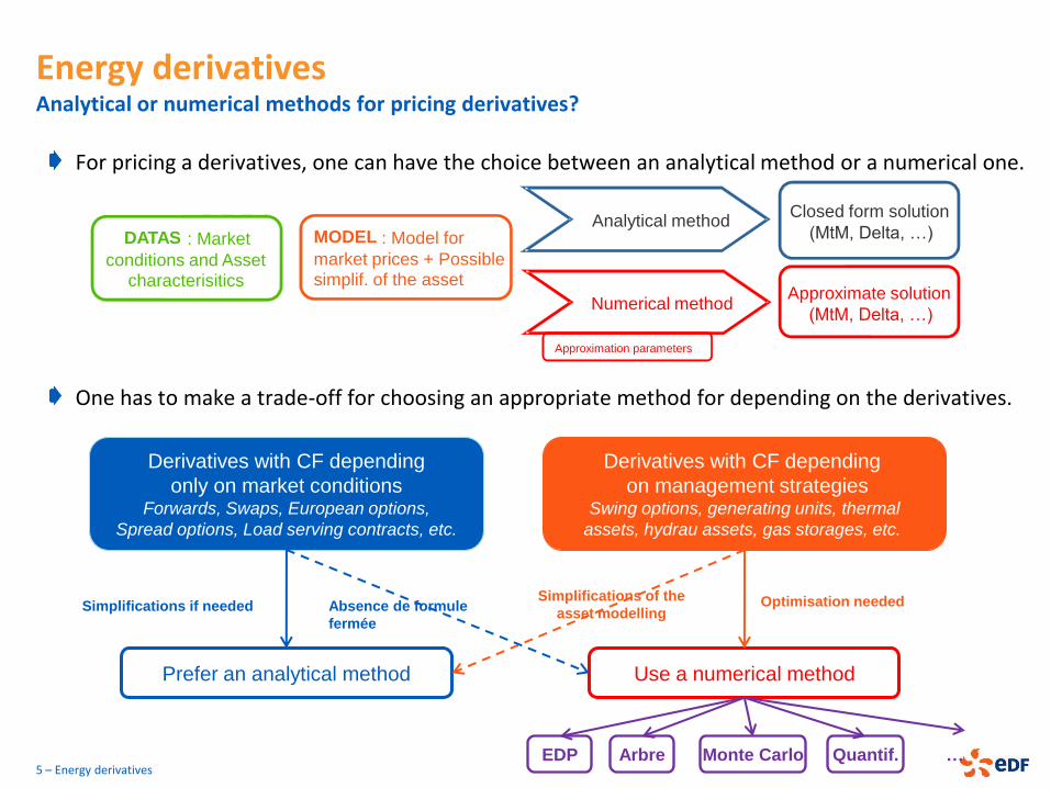
Energy derivatives Analytical or numerical methods for pricing derivatives?
For pricing a derivatives, one can have the choice between an analytical method or a numerical one.
One has to make a trade-off for choosing an appropriate method for depending on the derivatives.
Derivatives with CF depending
only on market conditions Forwards, Swaps, European options,
Spread options, Load serving contracts, etc.
Derivatives with CF depending
on management strategies Swing options, generating units, thermal
assets, hydrau assets, gas storages, etc.
Use a numerical method Prefer an analytical method
Simplifications of the
asset modelling Absence de formule
fermée
Optimisation needed Simplifications if needed
Monte Carlo EDP Arbre Quantif. … 5 – Energy derivatives
Numerical method
DATAS : Market
conditions and Asset characterisitics
Approximation parameters
MODEL : Model for
market prices + Possible simplif. of the asset
Analytical method
Approximate solution
(MtM, Delta, …)
Closed form solution
(MtM, Delta, …)
ENERGY DERIVATIVES
A typical energy portfolio
Forwards, Swaps and Spreads
Power plant modelling, Spread options pricing
Gas storage modelling
Swing options pricing
Load curve contract modelling
6 – Energy derivatives
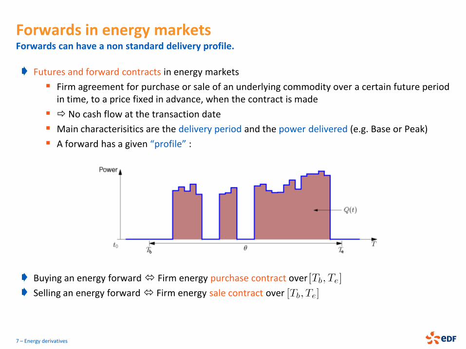
Forwards in energy markets Forwards can have a non standard delivery profile.
Futures and forward contracts in energy markets
Firm agreement for purchase or sale of an underlying commodity over a certain future period in time, to a price fixed in advance, when the contract is made
No cash flow at the transaction date
Main characterisitics are the delivery period and the power delivered (e.g. Base or Peak)
A forward has a given “profile” :
Buying an energy forward Firm energy purchase contract over
Selling an energy forward Firm energy sale contract over
7 – Energy derivatives
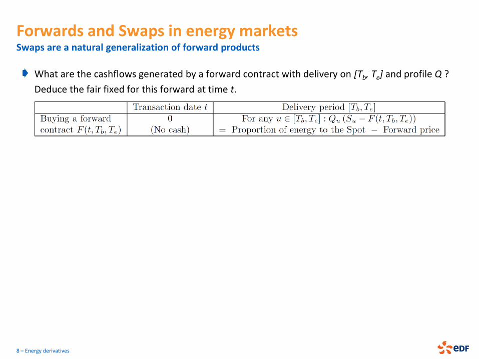
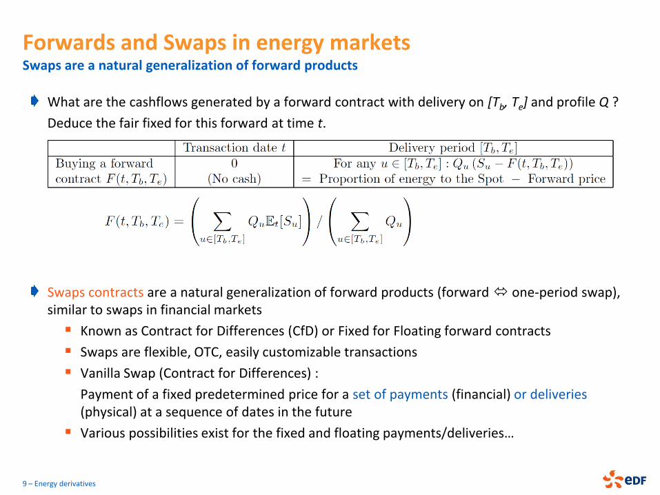
Forwards and Swaps in energy markets Swaps are a natural generalization of forward products
What are the cashflows generated by a forward contract with delivery on [Tb, Te] and profile Q ?
Deduce the fair fixed for this forward at time t.
8 – Energy derivatives
Forwards and Swaps in energy markets Swaps are a natural generalization of forward products
What are the cashflows generated by a forward contract with delivery on [Tb, Te] and profile Q ?
Deduce the fair fixed for this forward at time t.
Swaps contracts are a natural generalization of forward products (forward one-period swap), similar to swaps in financial markets
Known as Contract for Differences (CfD) or Fixed for Floating forward contracts
Swaps are flexible, OTC, easily customizable transactions
Vanilla Swap (Contract for Differences) :
Payment of a fixed predetermined price for a set of payments (financial) or deliveries (physical) at a sequence of dates in the future
Various possibilities exist for the fixed and floating payments/deliveries…
9 – Energy derivatives
Swaps in energy markets Some practice…
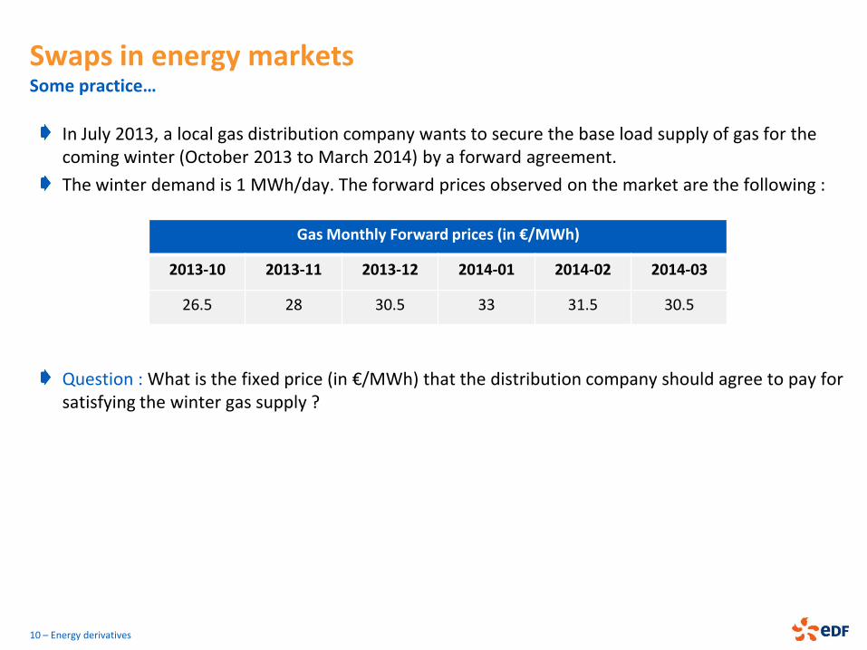
In July 2013, a local gas distribution company wants to secure the base load supply of gas for the coming winter (October 2013 to March 2014) by a forward agreement.
The winter demand is 1 MWh/day. The forward prices observed on the market are the following :
Question : What is the fixed price (in €/MWh) that the distribution company should agree to pay for satisfying the winter gas supply ?
10 – Energy derivatives
Gas Monthly Forward prices (in €/MWh)
2013-10 2013-11 2013-12 2014-01 2014-02 2014-03
26.5 28 30.5 33 31.5 30.5
Swaps in energy markets Some practice…
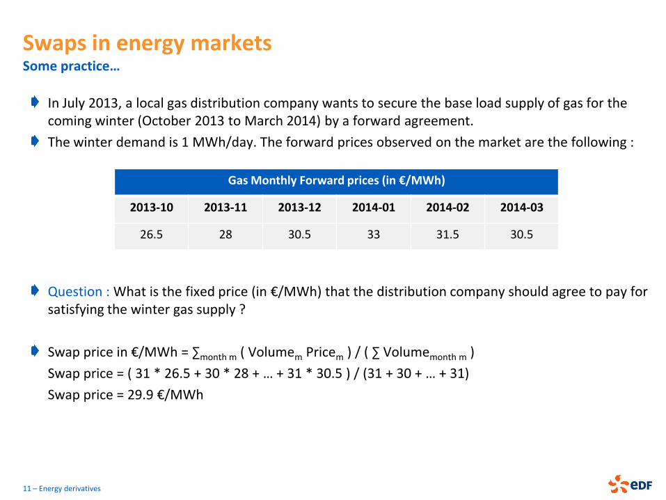
In July 2013, a local gas distribution company wants to secure the base load supply of gas for the coming winter (October 2013 to March 2014) by a forward agreement.
The winter demand is 1 MWh/day. The forward prices observed on the market are the following :
Question : What is the fixed price (in €/MWh) that the distribution company should agree to pay for satisfying the winter gas supply ?
Swap price in €/MWh = ∑month m ( Volumem Pricem ) / ( ∑ Volumemonth m )
Swap price = ( 31 * 26.5 + 30 * 28 + … + 31 * 30.5 ) / (31 + 30 + … + 31)
Swap price = 29.9 €/MWh
11 – Energy derivatives
Gas Monthly Forward prices (in €/MWh)
2013-10 2013-11 2013-12 2014-01 2014-02 2014-03
26.5 28 30.5 33 31.5 30.5
Spreads in energy markets Spreads are one of the most useful instrument in the “energy world”.
Spread : price differential between two commodities viewed as 2 points of the energy price system
Spreads can be used to describe power plants, refineries, storage facilities, etc.
There are four classes of Spreads : 1. Intra-commodity spread
Ex. Spread on oils with different qualities
2. Inter-commodity spread : price differential between two different but related commodities
Between two operational inputs or two operational outputs or between inputs and outputs (processing spread)
Crack Spread : gasoline or heating oil (refined products) versus crude oil (input)
Spark Spread : electricity versus a primary fuel (gas, oil, fuel oil, uranium)
Dark Spread : electricity versus coal
Clean XY Spread : X versus Y compensated for the price of CO2
3. Time or calendar spread
Ex. Summer 2014 versus Winter 2014
4. Geographic spread : difference between prices of a same product in two different locations
12 – Energy derivatives
Spark and Dark spreads… Practical application
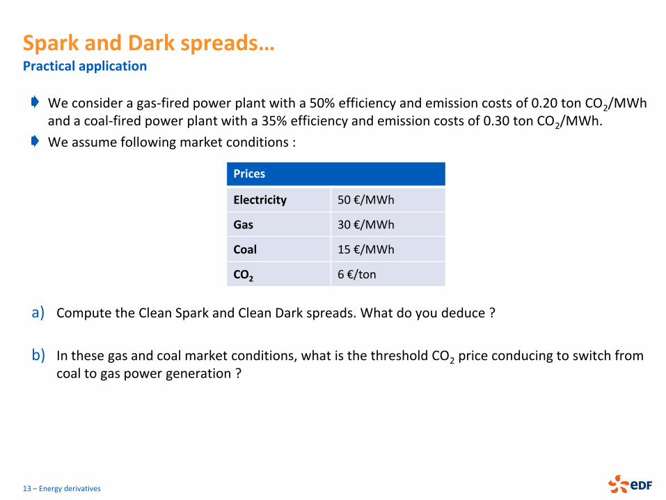
We consider a gas-fired power plant with a 50% efficiency and emission costs of 0.20 ton CO2/MWh and a coal-fired power plant with a 35% efficiency and emission costs of 0.30 ton CO2/MWh.
We assume following market conditions :
a) Compute the Clean Spark and Clean Dark spreads. What do you deduce ?
b) In these gas and coal market conditions, what is the threshold CO2 price conducing to switch from coal to gas power generation ?
13 – Energy derivatives
Prices
Electricity 50 €/MWh
Gas 30 €/MWh
Coal 15 €/MWh
CO2 6 €/ton
Spark and Dark spreads… Practical application
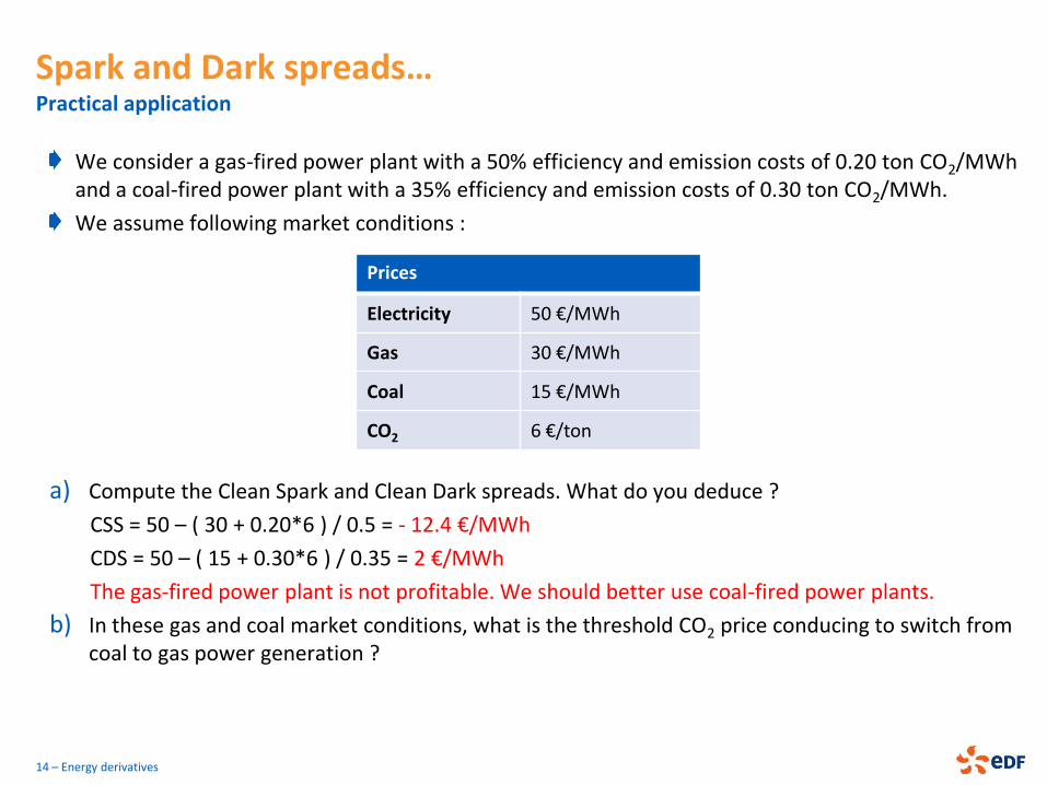
We consider a gas-fired power plant with a 50% efficiency and emission costs of 0.20 ton CO2/MWh and a coal-fired power plant with a 35% efficiency and emission costs of 0.30 ton CO2/MWh.
We assume following market conditions :
a) Compute the Clean Spark and Clean Dark spreads. What do you deduce ?
CSS = 50 – ( 30 + 0.20*6 ) / 0.5 = - 12.4 €/MWh
CDS = 50 – ( 15 + 0.30*6 ) / 0.35 = 2 €/MWh
The gas-fired power plant is not profitable. We should better use coal-fired power plants.
b) In these gas and coal market conditions, what is the threshold CO2 price conducing to switch from coal to gas power generation ?
14 – Energy derivatives
Prices
Electricity 50 €/MWh
Gas 30 €/MWh
Coal 15 €/MWh
CO2 6 €/ton
Spark and Dark spreads… Practical application
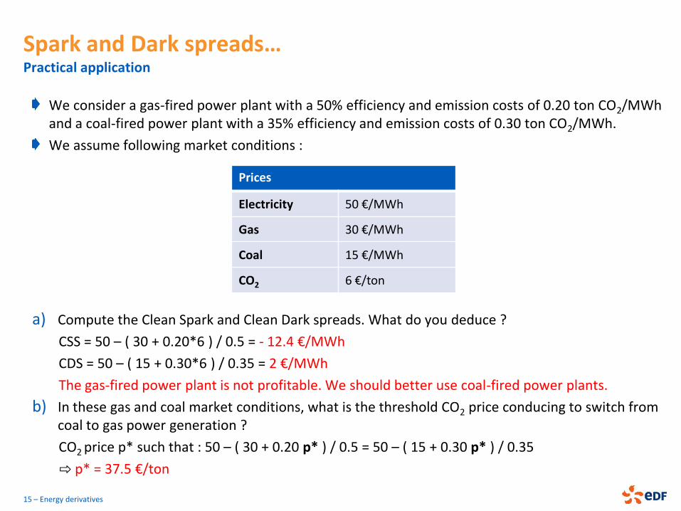
We consider a gas-fired power plant with a 50% efficiency and emission costs of 0.20 ton CO2/MWh and a coal-fired power plant with a 35% efficiency and emission costs of 0.30 ton CO2/MWh.
We assume following market conditions :
a) Compute the Clean Spark and Clean Dark spreads. What do you deduce ?
CSS = 50 – ( 30 + 0.20*6 ) / 0.5 = - 12.4 €/MWh
CDS = 50 – ( 15 + 0.30*6 ) / 0.35 = 2 €/MWh
The gas-fired power plant is not profitable. We should better use coal-fired power plants.
b) In these gas and coal market conditions, what is the threshold CO2 price conducing to switch from coal to gas power generation ?
CO2 price p* such that : 50 – ( 30 + 0.20 p* ) / 0.5 = 50 – ( 15 + 0.30 p* ) / 0.35
⇨ p* = 37.5 €/ton
15 – Energy derivatives
Prices
Electricity 50 €/MWh
Gas 30 €/MWh
Coal 15 €/MWh
CO2 6 €/ton
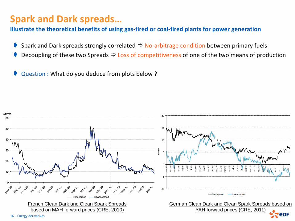
Spark and Dark spreads… Illustrate the theoretical benefits of using gas-fired or coal-fired plants for power generation
Spark and Dark spreads strongly correlated No-arbitrage condition between primary fuels
Decoupling of these two Spreads Loss of competitiveness of one of the two means of production
Question : What do you deduce from plots below ?
16 – Energy derivatives
German Clean Dark and Clean Spark Spreads based on
YAH forward prices (CRE, 2011)
French Clean Dark and Clean Spark Spreads
based on MAH forward prices (CRE, 2010)
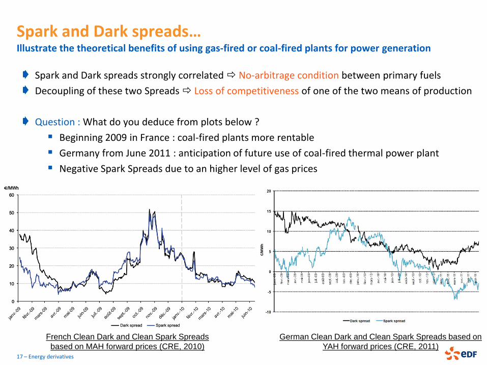
Spark and Dark spreads… Illustrate the theoretical benefits of using gas-fired or coal-fired plants for power generation
Spark and Dark spreads strongly correlated No-arbitrage condition between primary fuels
Decoupling of these two Spreads Loss of competitiveness of one of the two means of production
Question : What do you deduce from plots below ?
Beginning 2009 in France : coal-fired plants more rentable
Germany from June 2011 : anticipation of future use of coal-fired thermal power plant
Negative Spark Spreads due to an higher level of gas prices
17 – Energy derivatives
German Clean Dark and Clean Spark Spreads based on
YAH forward prices (CRE, 2011)
French Clean Dark and Clean Spark Spreads
based on MAH forward prices (CRE, 2010)
Transmission contracts Valuation as commodity derivatives
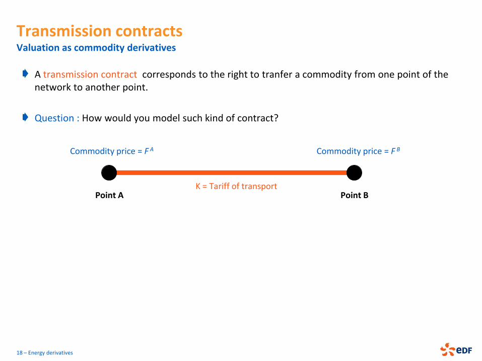
A transmission contract corresponds to the right to tranfer a commodity from one point of the network to another point.
Question : How would you model such kind of contract?
18 – Energy derivatives
Point A Point B K = Tariff of transport
Commodity price = F A Commodity price = F B
Transmission contracts Valuation as commodity derivatives
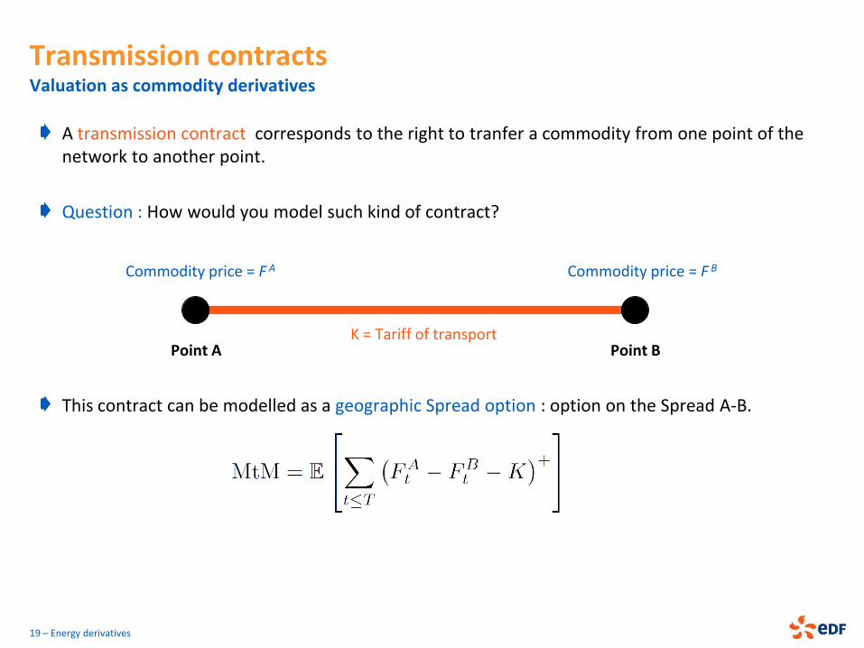
A transmission contract corresponds to the right to tranfer a commodity from one point of the network to another point.
Question : How would you model such kind of contract?
This contract can be modelled as a geographic Spread option : option on the Spread A-B.
19 – Energy derivatives
Point A Point B K = Tariff of transport
Commodity price = F A Commodity price = F B
ENERGY DERIVATIVES
A typical energy portfolio
Forwards, Swaps and Spreads
Power plant modelling, Spread options pricing
Gas storage modelling
Swing options pricing
Load curve contract modelling
20 – Energy derivatives
Power plants Power generating units can be viewed as derivatives.
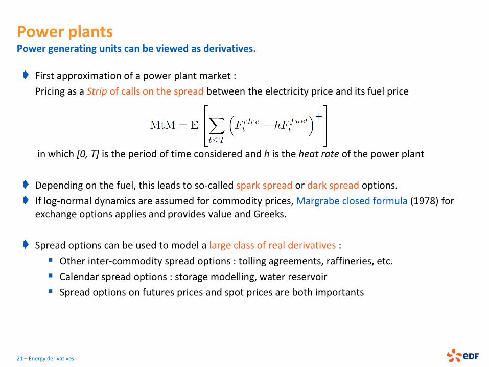
First approximation of a power plant market :
Pricing as a Strip of calls on the spread between the electricity price and its fuel price
in which [0, T] is the period of time considered and h is the heat rate of the power plant
Depending on the fuel, this leads to so-called spark spread or dark spread options.
If log-normal dynamics are assumed for commodity prices, Margrabe closed formula (1978) for exchange options applies and provides value and Greeks.
Spread options can be used to model a large class of real derivatives :
Other inter-commodity spread options : tolling agreements, raffineries, etc.
Calendar spread options : storage modelling, water reservoir
Spread options on futures prices and spot prices are both importants
21 – Energy derivatives
Power plants More complex pricing methods are required to model more realistic power plants.
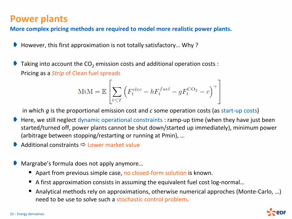
However, this first approximation is not totally satisfactory… Why ?
Taking into account the CO2 emission costs and additional operation costs :
Pricing as a Strip of Clean fuel spreads
in which g is the proportional emission cost and c some operation costs (as start-up costs)
Here, we still neglect dynamic operational constraints : ramp-up time (when they have just been started/turned off, power plants cannot be shut down/started up immediately), minimum power (arbitrage between stopping/restarting or running at Pmin), …
Additional constraints Lower market value
Margrabe’s formula does not apply anymore…
Apart from previous simple case, no closed-form solution is known.
A first approximation consists in assuming the equivalent fuel cost log-normal…
Analytical methods rely on approximations, otherwise numerical approches (Monte-Carlo, …) need to be use to solve such a stochastic control problem.
22 – Energy derivatives
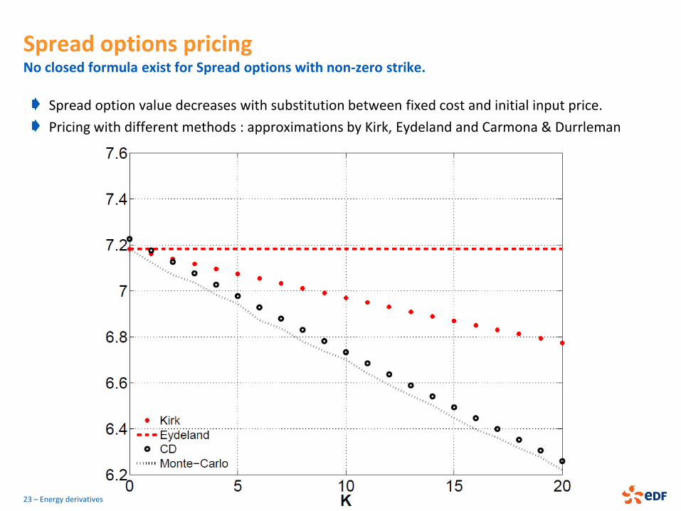
Spread options pricing No closed formula exist for Spread options with non-zero strike.
Spread option value decreases with substitution between fixed cost and initial input price.
Pricing with different methods : approximations by Kirk, Eydeland and Carmona & Durrleman
23 – Energy derivatives
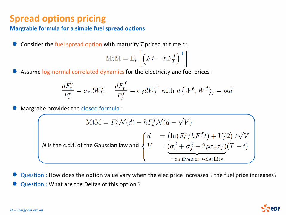
Spread options pricing Margrable formula for a simple fuel spread options
Consider the fuel spread option with maturity T priced at time t :
Assume log-normal correlated dynamics for the electricity and fuel prices :
Margrabe provides the closed formula :
N is the c.d.f. of the Gaussian law and
Question : How does the option value vary when the elec price increases ? the fuel price increases?
Question : What are the Deltas of this option ?
24 – Energy derivatives
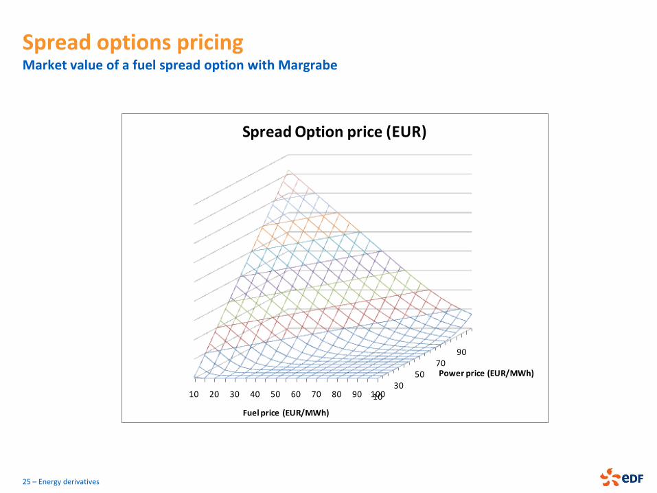
Spread options pricing Market value of a fuel spread option with Margrabe
25 – Energy derivatives
1030
5070
90
10 20 30 40 50 60 70 80 90 100
Power price (EUR/MWh)
Fuel price (EUR/MWh)
Spread Option price (EUR)
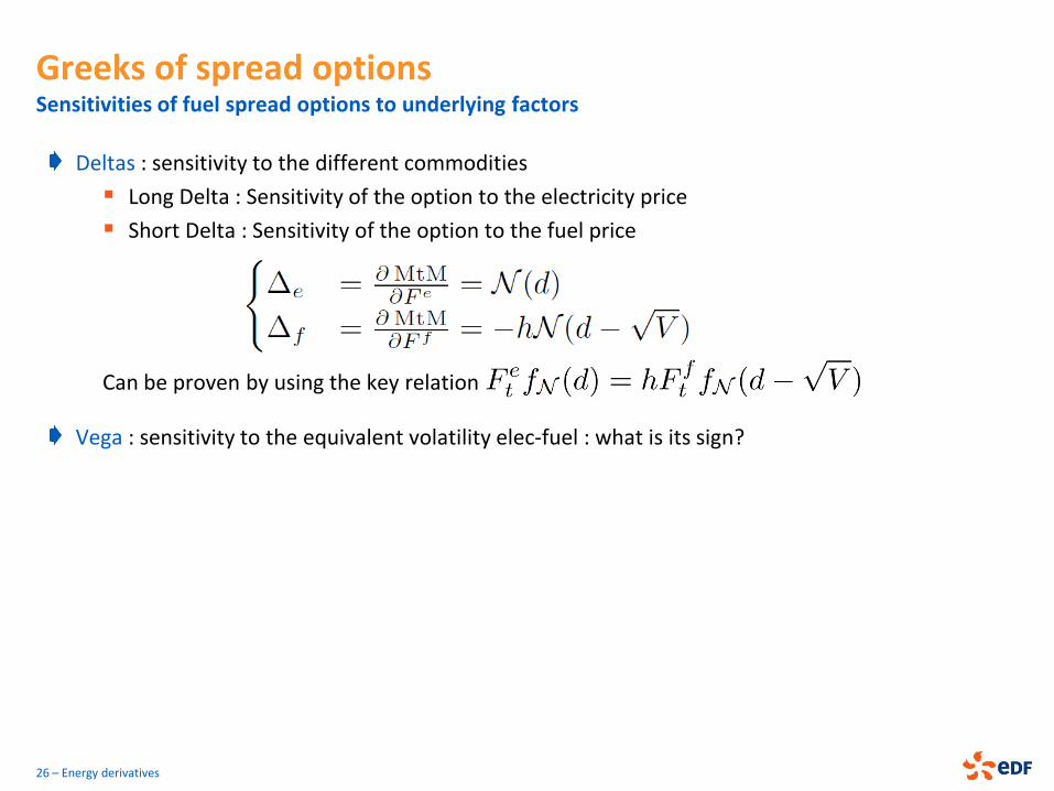
Greeks of spread options Sensitivities of fuel spread options to underlying factors
Deltas : sensitivity to the different commodities
Long Delta : Sensitivity of the option to the electricity price
Short Delta : Sensitivity of the option to the fuel price
Can be proven by using the key relation
Vega : sensitivity to the equivalent volatility elec-fuel : what is its sign?
26 – Energy derivatives

Greeks of spread options Sensitivities of fuel spread options to underlying factors
Deltas : sensitivity to the different commodities
Long Delta : Sensitivity of the option to the electricity price
Short Delta : Sensitivity of the option to the fuel price
Can be proven by using the key relation
Vega : sensitivity to the equivalent volatility elec-fuel : what is its sign?
Correlation Delta : sensitivity to the correlation between elec and fuel prices : what is its sign?
27 – Energy derivatives
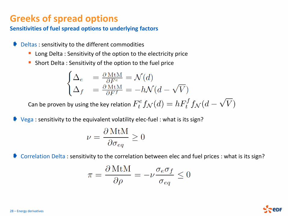
Greeks of spread options Sensitivities of fuel spread options to underlying factors
Deltas : sensitivity to the different commodities
Long Delta : Sensitivity of the option to the electricity price
Short Delta : Sensitivity of the option to the fuel price
Can be proven by using the key relation
Vega : sensitivity to the equivalent volatility elec-fuel : what is its sign?
Correlation Delta : sensitivity to the correlation between elec and fuel prices : what is its sign?
28 – Energy derivatives
29 – Energy derivatives
1030
5070
90
102030405060708090100
Power price (EUR/MWh)
Fuel price (EUR/MWh)
Power Delta (MW)
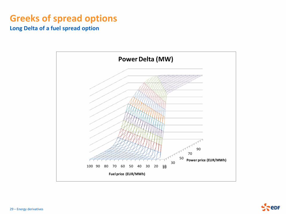
Greeks of spread options Long Delta of a fuel spread option
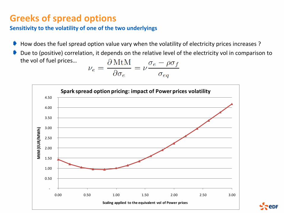
Greeks of spread options Sensitivity to the volatility of one of the two underlyings
How does the fuel spread option value vary when the volatility of electricity prices increases ?
Due to (positive) correlation, it depends on the relative level of the electricity vol in comparison to the vol of fuel prices…
-
0.50
1.00
1.50
2.00
2.50
3.00
3.50
4.00
4.50
0.00 0.50 1.00 1.50 2.00 2.50 3.00
MtM
(EU
R/M
Wh
)
Scaling applied to the equivalent vol of Power prices
Spark spread option pricing: impact of Power prices volatility
ENERGY DERIVATIVES
A typical energy portfolio
Forwards, Swaps and Spreads
Power plant modelling, Spread options pricing
Gas storage modelling
Swing options pricing
Load curve contract modelling
31 – Energy derivatives
Storages Storages are a major component of the gas chain
Why using storage facilities?
1. Physical and economic reasons (cost minimization)
Gas demand: variable (summer/winter) and inelastic
Inflexible gas supply: limited by the capacity of the pipeline system
Storages are closer to consumption areas
They ensure that gas will be easily accessible in response to higher demand
Interesting for non-producer countries with a high level of gas importation to reduce their dependance to producers
2. Regulation conditions
Gas supply compagnies have the obligation to own storage facilities to secure supply in periods of high demand
3. Financial reasons : arbitrage mechanism
Take benefit of the possible arbitrage between summer/winter or week-end/open days
Exploit market opportunities: inject gas in the storage while the gas is cheaper and withdraw it during periods with higher prices
Used for high consumption periods in gas but also for firing gas power plants (CCGT)
32 – Energy derivatives

Gas storages The storage has a strategic role for gas supply.
Storage is used by supply companies to store an extra gas capacity (issued from production fields or importations).
This buffer stock allows to hedge a part of the price risk (unexpected high demand).
The storage has thus an effect on the summer-winter spread.
33 – Energy derivatives
Injections in storages increase the global
demand thus increase the gas prices
Time
Price Withdrawals from storages increase the available
supply and decrease the gas prices
Winter Summer
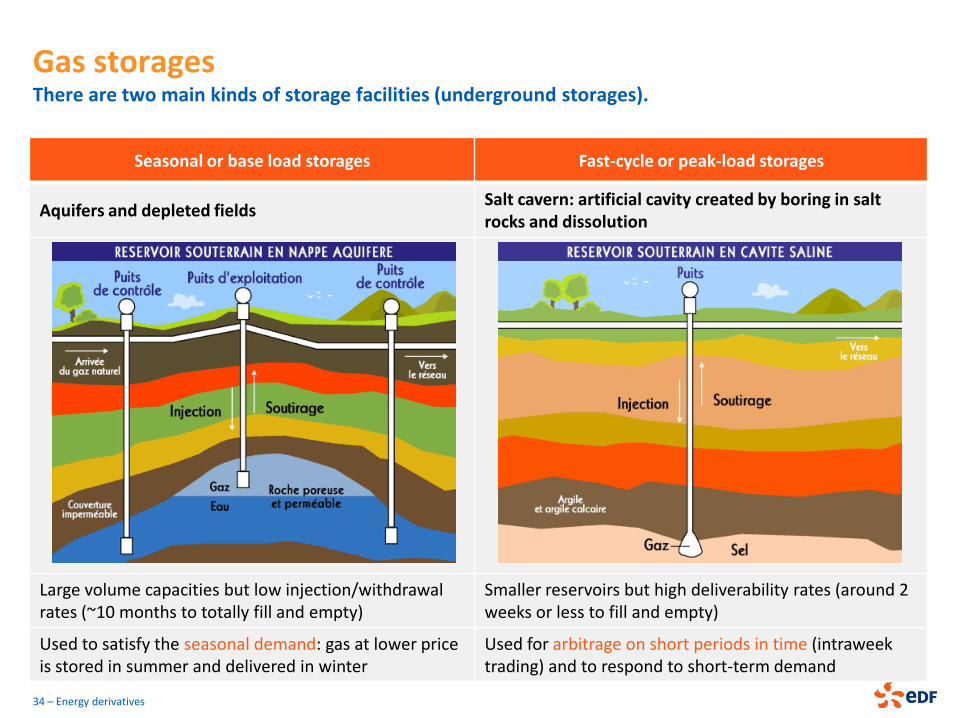
Gas storages There are two main kinds of storage facilities (underground storages).
34 – Energy derivatives
Seasonal or base load storages Fast-cycle or peak-load storages
Aquifers and depleted fields Salt cavern: artificial cavity created by boring in salt rocks and dissolution
Large volume capacities but low injection/withdrawal rates (~10 months to totally fill and empty)
Smaller reservoirs but high deliverability rates (around 2 weeks or less to fill and empty)
Used to satisfy the seasonal demand: gas at lower price is stored in summer and delivered in winter
Used for arbitrage on short periods in time (intraweek trading) and to respond to short-term demand
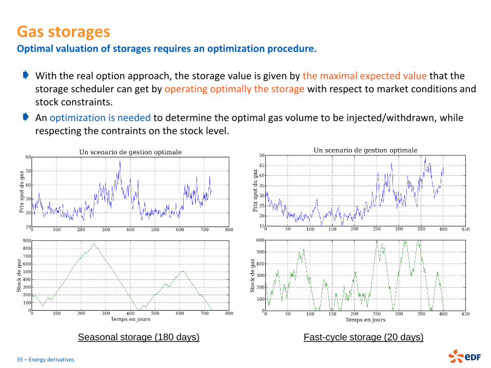
Gas storages Optimal valuation of storages requires an optimization procedure.
With the real option approach, the storage value is given by the maximal expected value that the storage scheduler can get by operating optimally the storage with respect to market conditions and stock constraints.
An optimization is needed to determine the optimal gas volume to be injected/withdrawn, while respecting the contraints on the stock level.
35 – Energy derivatives
Seasonal storage (180 days) Fast-cycle storage (20 days)
ENERGY DERIVATIVES
A typical energy portfolio
Forwards, Swaps and Spreads
Power plant modelling, Spread options pricing
Gas storage modelling
Swing options pricing
Load curve contract modelling
36 – Energy derivatives
Swing options in energy markets Many physical or financial assets including an optionality can be considered as Swing options
What is a Swing option ?
Right to receive/purchase a given volume of energy
Maximal number of ‘exercise’ rights nmax before the maturity
The exchange price (strike) can be fixed, variable or random.
Can be viewed as a multiple-exercise American options
More complex Swing options include a variable volume : can be “swing up” or “swing down”
In this case, global volume constraints impose a limited total energy amount
Swing options include a large class of structured assets in energy markets…
Gas supply contracts including Take-or-Pay clauses
Options to shut down services, demand-side mgmt contracts
Storage facilities (but allow both injections and withdrawals)
Water reservoirs, hydraulic assets (but include inflows)
37 – Energy derivatives
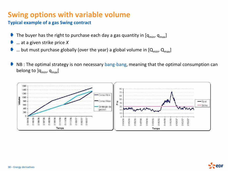
Swing options with variable volume Typical example of a gas Swing contract
The buyer has the right to purchase each day a gas quantity in [qmin, qmax]
… at a given strike price X
… but must purchase globally (over the year) a global volume in [Qmin, Qmax]
NB : The optimal strategy is non necessary bang-bang, meaning that the optimal consumption can belong to ]qmin, qmax[
38 – Energy derivatives
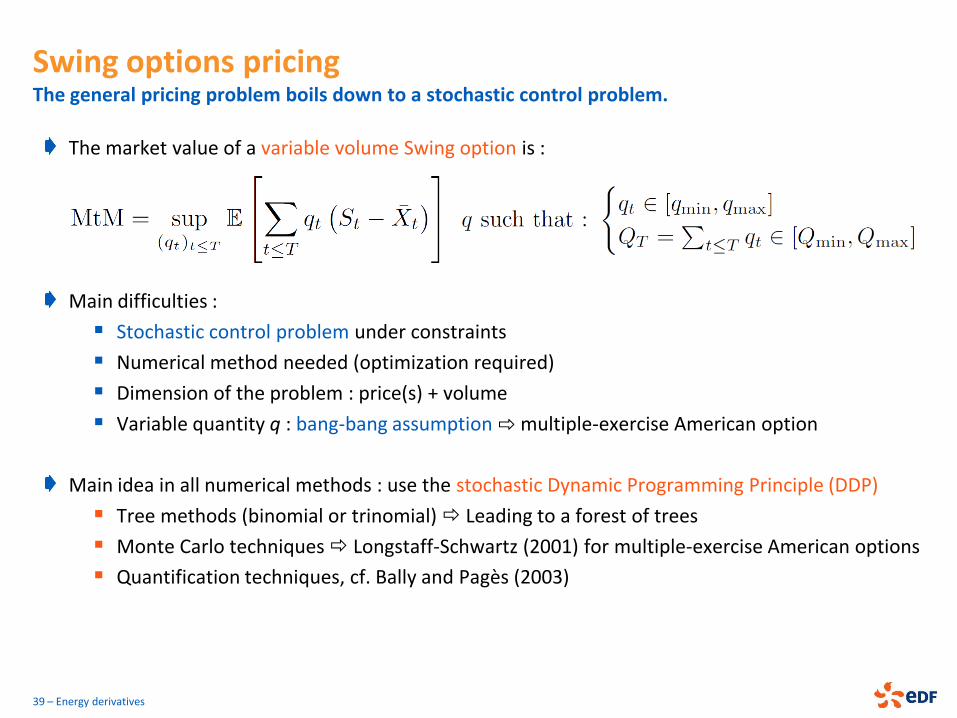
The market value of a variable volume Swing option is :
Main difficulties :
Stochastic control problem under constraints
Numerical method needed (optimization required)
Dimension of the problem : price(s) + volume
Variable quantity q : bang-bang assumption ⇨ multiple-exercise American option
Main idea in all numerical methods : use the stochastic Dynamic Programming Principle (DDP)
Tree methods (binomial or trinomial) Leading to a forest of trees
Monte Carlo techniques Longstaff-Schwartz (2001) for multiple-exercise American options
Quantification techniques, cf. Bally and Pagès (2003)
39 – Energy derivatives
Swing options pricing The general pricing problem boils down to a stochastic control problem.
Consider a gas Swing option over 180 days such that the minimal daily quantity is 10 MWh/day, the maximal daily quantity is 50 MWh/day and the global maximal quantity that can be purchased over the whole period is 6000 MWh.
After a standard normalization, this contract is usually separated into a firm Swap contract and a normalized Swing option.
a) What is the baseload volume provided by the Swap contract ? b) What is the remaining optional volume ? c) How many exercise rights are provided by the normalized Swing option ? d) Is the bang-bang assumption satisfied ?
Swing with q ∊ [qmin, qmax] Swap purchasing qmin every day + Purely Swing with q* ∊ [0, qmax – qmin]
40 – Energy derivatives
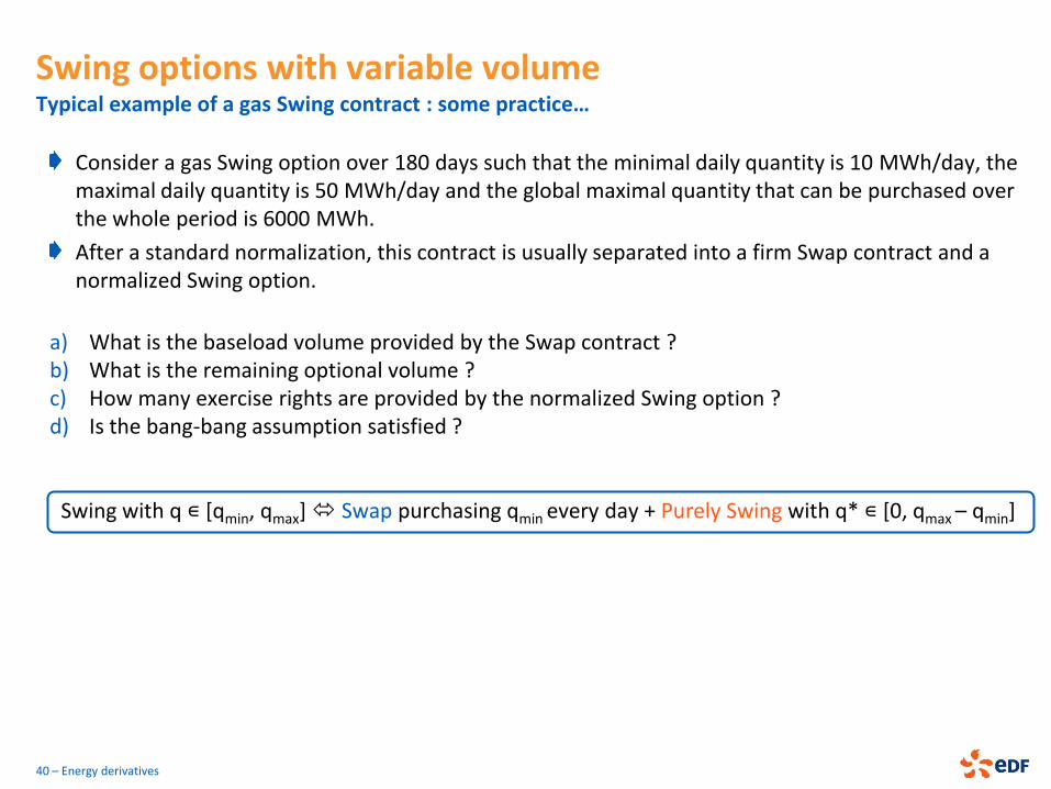
Swing options with variable volume Typical example of a gas Swing contract : some practice…

Consider a gas Swing option over 180 days such that the minimal daily quantity is 10 MWh/day, the maximal daily quantity is 50 MWh/day and the global maximal quantity that can be purchased over the whole period is 6000 MWh.
After a standard normalization, this contract is usually separated into a firm Swap contract and a normalized Swing option.
a) What is the baseload volume provided by the Swap contract ? b) What is the remaining optional volume ? c) How many exercise rights are provided by the normalized Swing option ? d) Is the bang-bang assumption satisfied ?
Swing with q ∊ [qmin, qmax] Swap purchasing qmin every day + Purely Swing with q* ∊ [0, qmax – qmin]
a) Baseload volume = 10 * 180 = 1800 MWh b) Remaining optional volume = 6000 – 1800 = 4200 MWh c) Number of exercise rights = 4200 / (50 – 10) = 105 times d) Yes, since there is an “integer” number of exercises in the Swing option
41 – Energy derivatives
Swing options with variable volume Typical example of a gas Swing contract : some practice…
42 – Energy derivatives
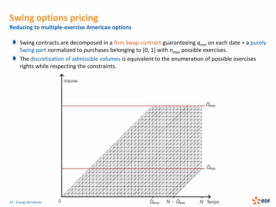
Swing options pricing Reducing to multiple-exercise American options
Swing contracts are decomposed in a firm Swap contract guaranteeing qmin on each date + a purely Swing part normalized to purchases belonging to [0, 1] with nmax possible exercises.
The discretization of admissible volumes is equivalent to the enumeration of possible exercises rights while respecting the constraints.
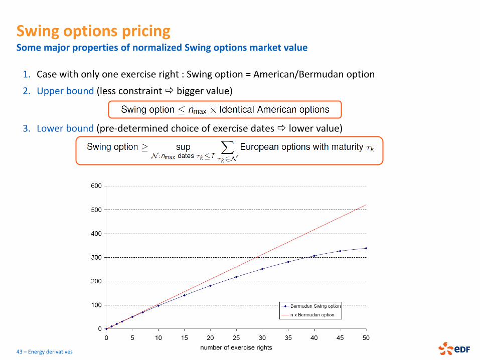
1. Case with only one exercise right : Swing option = American/Bermudan option
2. Upper bound (less constraint bigger value)
3. Lower bound (pre-determined choice of exercise dates lower value)
43 – Energy derivatives
Swing options pricing Some major properties of normalized Swing options market value
As multiple-exercise American options, Swing options can be valuate through :
Backward induction in time
An iteration on the number of exercise rights left
44 – Energy derivatives
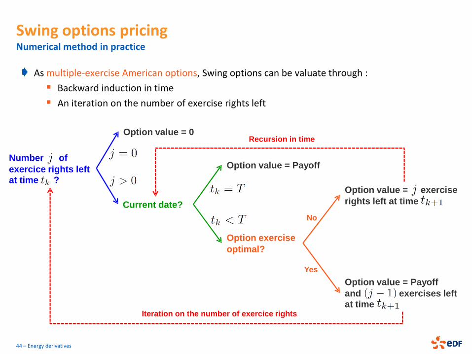
Swing options pricing Numerical method in practice
Number of
exercice rights left
at time ?
Option value = 0
Current date?
Option value = Payoff
Option exercise
optimal?
Option value = Payoff
and exercises left
at time
Option value = exercise
rights left at time
Yes
No
Iteration on the number of exercice rights
Recursion in time
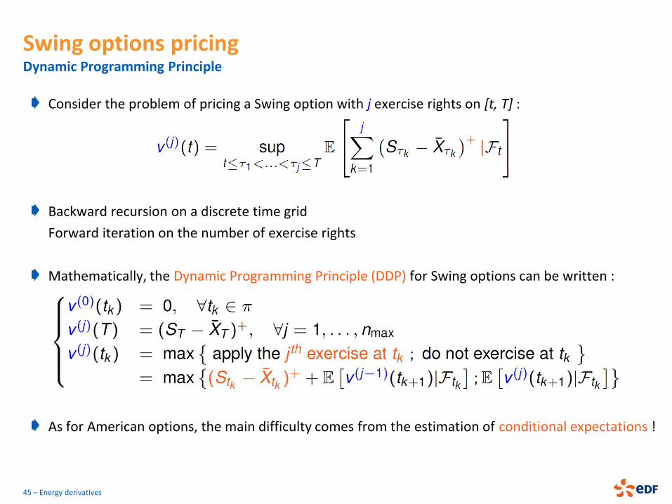
Consider the problem of pricing a Swing option with j exercise rights on [t, T] :
Backward recursion on a discrete time grid
Forward iteration on the number of exercise rights
Mathematically, the Dynamic Programming Principle (DDP) for Swing options can be written :
As for American options, the main difficulty comes from the estimation of conditional expectations !
45 – Energy derivatives
Swing options pricing Dynamic Programming Principle

Idea : representing the price evolution on a tree
Use of a binomial recombining tree
Possibility of upward and downward moves
At time ti the underlying price can take (i +1) values
46 – Energy derivatives
Swing options pricing Using tree method…

Example of trinominal recombining tree in a one factor model for gas prices :
47 – Energy derivatives
Swing options pricing Using tree method…
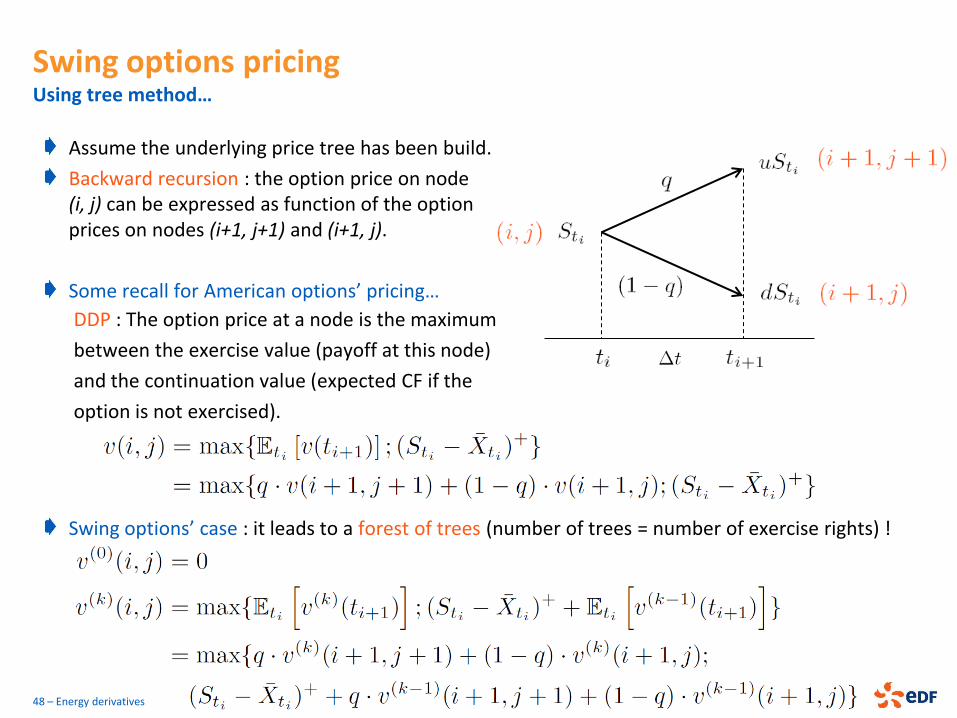
Assume the underlying price tree has been build.
Backward recursion : the option price on node (i, j) can be expressed as function of the option prices on nodes (i+1, j+1) and (i+1, j).
Some recall for American options’ pricing…
DDP : The option price at a node is the maximum
between the exercise value (payoff at this node)
and the continuation value (expected CF if the
option is not exercised).
Swing options pricing Using tree method…
48 – Energy derivatives
Swing options’ case : it leads to a forest of trees (number of trees = number of exercise rights) !
ENERGY DERIVATIVES
A typical energy portfolio
Forwards, Swaps and Spreads
Power plant modelling, Spread options pricing
Gas storage modelling
Swing options pricing
Load curve contract modelling
49 – Energy derivatives
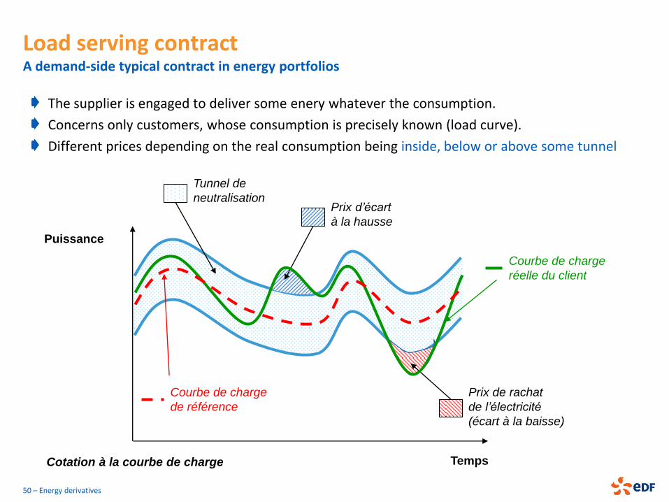
Load serving contract A demand-side typical contract in energy portfolios
The supplier is engaged to deliver some enery whatever the consumption.
Concerns only customers, whose consumption is precisely known (load curve).
Different prices depending on the real consumption being inside, below or above some tunnel
50 – Energy derivatives
Temps
Puissance
Tunnel de
neutralisation Prix d’écart
à la hausse
Prix de rachat
de l’électricité
(écart à la baisse)
Cotation à la courbe de charge
Courbe de charge
réelle du client
Courbe de charge
de référence