energy - e cient scheduling for cloud computing architectures
TRANSCRIPT

Technical University of Crete
Department of Electronic and Computer Engineering
Energy - Efficient Scheduling for CloudComputing Architectures
Diploma Thesis
Skevakis Emmanouil
Chania,
December 2012
1
Acknowledgements
First of all, I would like to express my sincere gratitude to my thesis supervisor, Polychro-
nis Koutsakis, whose expertise, understanding, and patience helped me complete my Diploma
thesis. I would also like to thank him for the opportunity he gave me, to work with him on my
thesis, and for his guidance through the last years of my undergraduate studies.
Furthermore, I would like to thank the members of my thesis examination committee, Prof.
Michael Paterakis and Prof. Minos Garofalakis for the time they devoted and their critical
evaluation.
My appreciation goes to Amir Sayegh, as well, for his participation in my thesis and for all
of his interesting ideas that led to the completion of this thesis.
Last but not least, I would like to thank my family and friends for their support and
encouragement through all these years.
2

Abstract
The rapid growth in demand for computational power driven by modern application ser-
vices along with the drop in storage and bandwidth pricing has led to the shift to the Cloud
Computing paradigm and to the establishment of large scale virtualized data centers, which
consume enormous amounts of electrical energy.
In our work, we focus on minimizing the energy consumption of cloud computing archi-
tectures using task consolidation and migration techniques. We also try to minimize the task
delays associated with the profit loss of the provider. We assume that a number of consumers
send their applications (tasks) and are processed by a number of resources that the provider
offers.
We first implemented an energy conscious task consolidation algorithm from the literature
on an extensive framework, the CloudSim ToolKit. We then designed and incorporated into
our system a live Virtual Machine migration process in order to reduce the energy consumed
by the system. As a last step, we implemented MinDelay, an algorithm which minimizes the
task delays while taking provider profit into account; we combined MinDelay with our energy-
efficient approach in order to study the potential gains of the hybrid scheme.
3

Contents
1 Introduction 5
1.1 What is Cloud Computing? . . . . . . . . . . . . . . . . . . . . . . . . . . . . . 5
1.2 Why do we need Cloud Computing? . . . . . . . . . . . . . . . . . . . . . . . . 5
1.3 Cloud Computing Models . . . . . . . . . . . . . . . . . . . . . . . . . . . . . . 6
1.4 Cloud Computing System Components . . . . . . . . . . . . . . . . . . . . . . . 8
1.5 Energy Problem . . . . . . . . . . . . . . . . . . . . . . . . . . . . . . . . . . . . 9
2 Simulation Tool - CloudSim 11
3 System Model 19
3.1 Cloud Model . . . . . . . . . . . . . . . . . . . . . . . . . . . . . . . . . . . . . 19
3.2 Application Model . . . . . . . . . . . . . . . . . . . . . . . . . . . . . . . . . . 19
3.3 Energy Model . . . . . . . . . . . . . . . . . . . . . . . . . . . . . . . . . . . . . 20
4 Task Consolidation 22
4.1 Energy Conscious Task Consolidation Algorithm - ECTC . . . . . . . . . . . . . 22
5 On the Potential of Simulated Annealing 25
5.1 Neighbour Search Techniques (NS) . . . . . . . . . . . . . . . . . . . . . . . . . 26
6 VM Live Migration 28
6.1 Migration Process . . . . . . . . . . . . . . . . . . . . . . . . . . . . . . . . . . . 29
6.2 Modified Best Fit Decreasing (MBFD) . . . . . . . . . . . . . . . . . . . . . . . 31
7 Profit - driven request scheduling (Min Delay) 33
8 Simulations 37
8.1 ECTC vs Random Assignment . . . . . . . . . . . . . . . . . . . . . . . . . . . . 38
8.1.1 Dynamic creation of hosts . . . . . . . . . . . . . . . . . . . . . . . . . . 38
4

8.1.2 Delaying Tasks . . . . . . . . . . . . . . . . . . . . . . . . . . . . . . . . 44
8.2 Activate Migrations vs Deactivate Migrations . . . . . . . . . . . . . . . . . . . 51
8.2.1 Dynamic creation of hosts . . . . . . . . . . . . . . . . . . . . . . . . . . 51
8.2.2 Delaying Tasks . . . . . . . . . . . . . . . . . . . . . . . . . . . . . . . . 58
9 Conclusions 65
5
1 Introduction
1.1 What is Cloud Computing?
In [1] the authors refer to cloud computing as “ the long-held dream of computing as a
utility, which has the potential to transform a large part of the Information Technology (IT)
industry, making software even more attractive as a service”. The Cloud Security Alliance, in
[2] states that “ the cloud describes the use of a collection of services, application and storage
resources ”. In this ideal concept of Cloud Computing, capacity seems infinite, scalability is
instantaneous and users only pay for what resource they use.
The National Institute of Standards and Technology (NIST) proposed the most broad accept-
able definition of cloud computing [3] and that is, “ a model for enabling convenient, on-demand
network access to a shared pool of configurable computing resources (such as networks, servers,
applications and services) that can be rapidly provisioned and released with minimal manage-
ment effort or service provider interaction”. This cloud model promotes availability and is
composed of five essential characteristics (On-demand self-service, Broad network access, Re-
source pooling, Rapid elasticity, Measured Service), three service models (Cloud Software as a
Service (SaaS), Cloud Platform as a Service (PaaS), Cloud Infrastructure as a Service (IaaS))
and four deployment models (Private cloud, Community cloud, Public cloud, Hybrid cloud).
The dramatic increase in cheap broadband wireless and wired network bandwidth along with
the drop in storage pricing has led to the practical fulfilment of the cloud computing idea. To-
day, cloud computing is gaining momentum as a business model that reduces capital investment
and reduces risk.
1.2 Why do we need Cloud Computing?
Cloud computing comes into focus when you think about what IT always needs : a way to
increase capacity or add capabilities on the fly without investing in new infrastructure, training
new personnel, or licensing new software. Cloud computing encompasses any subscription-based
6

or pay-per-use service that, in real time over the Internet, extends IT’s existing capabilities
[4]. The cloud does seem to solve some long-standing issues with the ever increasing costs
of implementing, maintaining, and supporting an IT infrastructure that is seldom utilized
anywhere near its capacity in the single-owner environment. There is an opportunity to increase
efficiency and reduce costs in the IT portion of the business and decision-makers are beginning
to pay attention [5]. Cloud computing intends to make the Internet the ultimate home of all
computing resources (storage, computations, applications) and allow end users (both individuals
and business) to take advantage of these resources in quantities of their choice, location of their
preferences, for the duration of their liking. The world web can become the provision store for
all our computing needs [6].
1.3 Cloud Computing Models
There are 3 fundamental models, according to which, cloud providers offer their services.
These models are Infrastructure as a Service (IaaS), Platform as a Service (PaaS) and Software
as a Service (SaaS) [7].
IaaS refers to the capability provided by the cloud provider to the end user for provision
processing, storage, networks and other fundamental computing resources. The user is able
to deploy and run software, such as applications and operating systems. He does not manage
or control the physical infrastructure of the cloud, but controls operating systems, storage,
deployed applications and has limited control of select networking components usually on a
pay-per-use model. To deploy their applications, users install operating system images and
their application software on the cloud infrastructure.
Examples of IaaS include Amazon EC2, Windows Azure, HP Cloud.
PaaS refers to the capability provided to the cloud user to deploy onto the cloud infras-
tructure user- created or acquired applications (on already installed platforms) using tools and
7

programming languages supported by the cloud provider. Users do not have to worry about
the cost of buying and managing the required hardware.
Examples of PaaS include Amazon Elastic Beanstalk, Goggle App Engine, Windows Azure
Compute.
Finally, SaaS refers to the capability provided to the user to use the provider’s applications,
already running on a cloud infrastructure. These applications are accessible from client devices
through a client interface, such as a web browser. The users rent the cloud’s application soft-
ware and databases usually per month or per year.
Examples of SaaS include Google Apps, Microsoft Office 365
Clouds aim to power the next generation data centers as the enabling platform for dynamic
and flexible application provisioning. This is facilitated by exposing data centers capabilities
as a network of virtual services so that users are able to access and deploy applications from
anywhere in the Internet driven by the demand and the QoS (Quality of Service) requirements.
Similarly, IT companies with innovative ideas for new application services are no longer required
to make large capital outlays in the hardware and software infrastructures. By using clouds
as the application hosting platform, IT companies are freed from the trivial task of setting
up basic hardware and software infrastructures. Thus they can focus more on innovation and
creation of business values for their application services.
There are four different deployment models used in cloud computing [8] : public cloud,
community cloud, hybrid cloud and private cloud. The differences between the four types are
based on the availability of the cloud. Public clouds are available to the general public, and
private clouds are available to an organization, whereas community clouds and hybrid clouds
are available to several organizations.
8

Public cloud : Applications, storage, and other resources are made available to the gen-
eral public by a service provider. These services are free or offered on a pay-per-use model.
Community cloud : Shares infrastructure between several organizations from a specific com-
munity with common interests and is hosted internally or externally. The costs are spread over
fewer users than a public cloud (but more than a private cloud), so only part of the cost savings
potential of cloud computing is realized.
Hybrid cloud : Consists of two or more clouds (private, community or public) that remain
unique entities but are bound together, offering the benefits of multiple deployment models.
Private cloud : Cloud infrastructure operated solely for a single organization, whether man-
aged internally or by a third-party and hosted internally or externally. Undertaking a private
cloud project requires a significant level and degree of engagement to virtualize the business en-
vironment, and it will require the organization to re-evaluate decisions about existing resources.
1.4 Cloud Computing System Components
A Cloud Computing (CC) system consists of several components. In a simple topologi-
cal sense, a CC system is made up of clients, datacenters, and physical resources (distributed
servers). Each of them has a specific role in order to deliver the functional application [9]
Clients are the devices that end-users use in order to manage their information on the cloud.
Such devices are PCs, laptops, PDAs, mobile phones or tablets. Clients can have a hard disk or
not. A client sends an application to the CC system’s provider specifying two constraints, time
and cost, which is later on processed by the system. Some cloud applications require specific
software to be installed on the client, whereas others just need a web browser.
9

Datacenters are collections of servers where the applications are processed. This can be a
large room, practically anywhere, full of servers that clients access through a network, usually
the Internet.
Physical Resources are servers usually placed in a datacenter but can be placed at dif-
ferent geographic locations, as well, and act like they were all placed in the same room. This
is done because if something went wrong at one server (or a group of servers placed in nearby
locations), other servers would still be accessible. Moreover, with virtualization techniques, we
can have many virtualized servers running on one physical server.
1.5 Energy Problem
The rapid growth in demand for computational power driven by modern service applica-
tions combined with the shift to the Cloud Computing model have led to the establishment
of large scale virtualized data centers. Data centers consume enormous amounts of electrical
energy resulting in high operating costs and carbon dioxide emissions. Researches from the
American Society of Heating, Refrigerating and Air-Conditioning Engineers (ASHRAE), in
[10] estimate that by the year 2014 infrastructure and energy costs will contribute about 75%
to the overall cost of an operating data center, whereas IT would contribute just 25% to the
overall cost [11]. In 2007 2% of the world’s total CO2 emissions were caused by the IT industry
and 1.5% of the total U.S. power consumption was by data centers (doubled since 2000). In
2010 the total energy bills for data centers was over 11 billion dollars and the energy costs in a
typical data center doubles every five years, according to the McKinsey report, [12]. Compute
resources and especially servers are the heart of the problem due to high operating and cooling
energy costs. The reason for this high energy consumption is not just the quantity of computing
resources but also the inefficient usage of these resources. Therefore we need to turn to solu-
tions, such as Green Cloud Computing, that do not only reduce electrical energy and carbon
emissions to the environment, but also reduce the operational costs of data centers. One of the
10

basic problems that contribute to the increase in energy consumption is that the utilization of
servers in data centers, rarely reaches 100%. Most servers operate at a utilization rate lower
than 50% and this leads to extra expenses. Additionally, servers on idle mode consume about
70% of their peak power. Thus, the need of keeping more servers switched off or at a lower
power mode and trying to achieve better utilization rates of switched on servers is imperative.
In this work we first we first implement the ECTC algorithm as presented in [13]. We focus
on minimizing the energy consumption of cloud computing architectures through decisions
made for task allocation and task migration. We used the CloudSim toolkit [14] in order to
implement the algorithms and evaluate them (whereas in [13]) the authors used a custom-made
simulation of theirs) via a widely used tool. We tested several scenarios which we present and
discuss in this thesis. The next chapters are organized as follows : in Chapter 2 we provide
an overview of the simulation tool we used and in Chapter 3 we analyse the system model
we used. In Chapter 4 we present the task consolidation problem and the ECTC algorithm.
Chapter 5 presents a method we used in order to obtain better results than ECTC and Chapter
6 presents our work on Virtual Machines (VMs) Live Migration. In Chapter 7 we incorporate
in our system an algorithm which focuses on minimizing the service delays. Chapter 8 presents
our results and Chapter 9 includes our conclusions.
11

2 Simulation Tool - CloudSim
For our simulations, we used CloudSim [14], a new generalized and extensible simulation
framework that allows seamless modelling, simulation and experimentation of emerging Cloud
computing infrastructures and application services. We modified and extended the CloudSim
Tool kit to implement our system model. The basic features that CloudSim offers are :
• Support for modelling and simulation of large scale Cloud computing environments, in-
cluding data centers, on a single physical computing node.
• Self-contained platform for modelling Clouds, service brokers, provisioning, and alloca-
tions policies.
• Support for simulation of network connections among the simulated system elements.
• Facility for simulation of federated Cloud environment that inter-networks resources from
both private and public domains.
• Availability of a virtualization engine that aids in creation and management of multiple,
independent, and co-hosted virtualized services on a data center node, and
• Flexibility to switch between space-shared and time-shared allocation of processing cores
to virtualized services.
Figure 1 shows the layered design of the Cloud computing architecture. Physical Cloud
resources along with core middleware capabilities form the basis for delivering IaaS and PaaS.
The user-level middleware aims at providing SaaS capabilities. The top layer focuses on applica-
tion services (SaaS) by making use of services provided by the lower layer services. PaaS/SaaS
services are often developed and provided by third party service providers, who are different
from the IaaS providers.
12

Figure 1: Layered Cloud Computing Architecture
Figure 2 shows the multi-layered design of the CloudSim software framework and its archi-
tectural components. Initial releases of CloudSim used SimJava, a discrete event simulation
engine that supports several core functionalities, such as queuing and processing of events,
creation of Cloud system entities (services, host, data center, broker, virtual machines), com-
munication between components, and management of the simulation clock.
The CloudSim simulation layer provides support for modelling and simulation of virtualized
Cloud-based data center environments including dedicated management interfaces for virtual
machines (VMs), memory, storage, and bandwidth. The fundamental issues such as provision-
ing of hosts to VMs, managing application execution, and monitoring dynamic system state are
handled by this layer. Cloud providers, who want to study the efficiency of different policies in
allocating their hosts to VMs (VM provisioning), would need to implement their strategies at
this layer. Such an implementation can be achieved by programmatically extending the core
VM provisioning functionality. There is a clear distinction at this layer related to provisioning
of hosts to VMs. A Cloud host can be concurrently allocated to a set of VMs that execute
applications based on SaaS providers defined QoS levels. This layer also exposes functionalities
that a Cloud application developer can extend to perform complex workload profiling and ap-
13

Figure 2: Layered CloudSim Architecture
plication performance studies. The top-most layer in the CloudSim stack is the User Code that
exposes basic entities for hosts (number of machines, their specification and so on), applications
(number of tasks and their requirements), VMs, number of users and their application types,
and broker scheduling policies. By extending the basic entities given at this layer, a Cloud
application developer can perform the following activities:
1. Generate a mix of workload request distributions and application configurations.
2. Model Cloud availability scenarios and perform robust tests based on the custom config-
urations.
3. Implement custom application provisioning techniques for clouds and their federation.
As Cloud computing is still an emerging paradigm for distributed computing, there is a
lack of defined standards, tools and methods that can efficiently tackle the infrastructure and
application level complexities. Hence, in the near future there will be a number of research
efforts both in academia and industry towards defining core algorithms, policies, and application
14

benchmarking based on execution contexts. By extending the basic functionalities already
exposed with CloudSim, researchers will be able to perform tests based on specific scenarios
and configurations, thereby allowing the development of the best practices in all of the critical
aspects related to Cloud Computing.
The infrastructure-level services (IaaS) related to the clouds can be simulated by extending
the Datacenter entity of CloudSim. The Data Center entity manages a number of host entities.
The hosts are assigned to one or more VMs based on a VM allocation policy that should be
defined by the Cloud service provider. Here, the VM policy stands for the operations control
policies related to VM life cycle such as: provisioning of a host to a VM, VM creation, VM
destruction, and VM migration. Similarly, one or more application services can be provisioned
within a single VM instance, referred to as application provisioning in the context of Cloud
computing. In the context of CloudSim, an entity is an instance of a component. A CloudSim
component can be a class (abstract or complete), or set of classes that represent one CloudSim
model (data center, host).
A Datacenter can manage several hosts that in turn manage VMs during their life cycles.
A Host is a CloudSim component that represents a physical computing server in a Cloud: it is
assigned a pre-configured processing capability (expressed in millions of instructions per second
MIPS), memory, storage, and a provisioning policy for allocating processing cores to virtual
machines. The Host component implements interfaces that support modelling and simulation
of both single-core and multi-core nodes.
VM allocation (provisioning) is the process of creating VM instances on hosts that match the
critical characteristics (storage, memory), configurations (software environment), and require-
ments (availability zone) of the SaaS provider. CloudSim does not enforce any limitation on the
service models or provisioning techniques that developers want to implement and perform tests
with. Once an application service is defined and modelled, it is assigned to one or more pre-
instantiated VMs through a service specific allocation policy. Allocation of application-specific
15

VMs to Hosts in a Cloud-based data center is the responsibility of a Virtual Machine Allocation
controller component (called VmAllocationPolicy). This component exposes a number of cus-
tom methods for researchers and developers that aid in the implementation of new policies based
on optimization goals (user centric, system centric or both). By default, VmAllocationPolicy
implements a straightforward policy that allocates VMs to the Host in First-Come-First-Served
(FCFS) basis. Hardware requirements such as the number of processing cores, memory and
storage form the basis for such provisioning. Other policies, including the ones likely to be ex-
pressed by Cloud providers, can also be easily simulated and modelled in CloudSim. However,
policies used by public Cloud providers (Amazon EC2, Microsoft Azure) are not publicly avail-
able, and thus a pre-implemented version of these algorithms is not provided with CloudSim.
For each Host component, the allocation of processing cores to VMs is done based on a
host allocation policy. This policy takes into account several hardware characteristics such as
number of CPU cores, CPU share, and amount of memory (physical and secondary) that are
allocated to a given VM instance. Hence, CloudSim supports several simulation scenarios that
assign specific CPU cores to specific VMs (a space-shared policy) or dynamically distribute the
capacity of a core among VMs (time-shared policy) and assign cores to VMs on demand. Each
Host component also instantiates a VM scheduler component, which can either implement the
space-shared or the time-shared policy for allocating cores to VMs. Fundamental software and
hardware configuration parameters related to VMs are defined in the VM class.
As we mentioned before, several classes of CloudSim were modified and basic functionalities
were extended in order to match our system model. The most important modifications we
made are analyzed at the end of this section. Some of the fundamental classes of CloudSim are
described below :
Datacenter : This class models the core infrastructure level services (hardware) that are
offered by Cloud providers. It encapsulates a set of compute hosts that can either be homoge-
16

neous or heterogeneous with respect to their hardware configurations (memory, cores, capacity
and storage). Furthermore, every Datacenter component instantiates a generalized application
provisioning component that implements a set of policies for allocating bandwidth, memory,
and storage devices to hosts and VMs.
Host : This class models a physical resource such as a compute or storage server. It
encapsulates important information such as the amount of memory and storage, a list and type
of processing cores (to represent a multi-core machine), an allocation of policy for sharing the
processing power among virtual machines, and policies for provisioning memory and bandwidth
to the virtual machines.
DatacenterBroker : This class models a broker, which is responsible for mediating negotia-
tions between SaaS and Cloud providers; and such negotiations are driven by QoS requirements.
The broker acts on behalf of SaaS providers. It discovers suitable Cloud service providers by
querying the Cloud Information Service (CIS) and undertakes on-line negotiations for allocation
of resources/services that can meet an application’s QoS requirements. The researchers and
system developers must extend this class for evaluating and testing custom brokering policies.
Cloudlet : This class models the Cloud-based application services (such as content deliv-
ery, social networking, and business workflow). CloudSim orchestrates the complexity of an
application in terms of its computational requirements. Every application service has a pre-
assigned instruction length and data transfer (both pre and post fetches) overhead that it needs
to undertake during its life-cycle. This class can also be extended to support modelling of other
performance and composition metrics for applications such as transactions in database-oriented
applications.
Vm : This class models a virtual machine, which is managed and hosted by a Cloud
host component. Every VM component has access to a component that stores the following
characteristics related to a VM: accessible memory, processor, storage size, and the VMs internal
provisioning policy that is extended from an abstract component called the CloudletScheduler.
17

CloudletScheduler : This abstract class is extended by implementation of different policies
that determine the share of processing power among Cloudlets in a virtual machine. Two types
of provisioning policies are offered: space-shared (CloudetSchedulerSpaceShared) and time-
shared (CloudletSchedulerTimeShared).
VmAllocationPolicy : VmAllocationPolicy is an abstract class that represents the provi-
sioning policy of hosts to virtual machines in a Datacenter. The chief functionality is to select
an available host in a data center that meets the memory, storage, and availability requirement
for a VM deployment. It supports a two-stage commitment of host’s reservation: first, the host
is reserved and, once the user commits, it is effectively allocated to the user.
VmScheduler : This is an abstract class implemented by a Host component that models
the policies (space-shared, time-shared) required for allocating processor cores to VMs. The
functionalities of this class can easily be overridden to accommodate application specific pro-
cessor sharing policies.
We created our own functions in the Datacenter class in order to measure the energy con-
sumption of the system and in order to create hosts dynamically (this option is analyzed in
section 8). We also modified the function updateCloudletProcessing(), which is responsible for
the VM migration process, for the need of the fourth step in the migration process (see Section
6.1).
A new function (processPeriodicCloudletCreation) was created in the DatacenterBroker class,
in order to create tasks dynamically (without this function all tasks would be created and sub-
mitted at the same time, at the beginning of the simulation). Another important function that
we created in this class is submitPeriodicCloudlets, which is responsible for submitting tasks
to the right resource. The right resource is found either from the ECTC algorithm (see Section
4.1) or from the MinDelay algorithm (see Section 7).
In the Host class, new functions were created in order to calculate the cost function of ECTC
(see Section 4.1) and in order to find which VM will serve each task.
18

Furthermore, modifications were made and new functions were created in the VmAllocatioPol-
icy class. The optimizeAllocation function was modified, a function responsible for finding the
Best Placement of VMs to hosts (see Section 6.1), and a few functions were created in order to
implement the four steps needed for our migration process (see Section 6.1).
19

3 System Model
In this section we describe our system model consisting of the cloud, the application
and the energy model. The details of the model presented in this section focus on resource
management characteristics and issues from a cloud provider’s perspective [13].
3.1 Cloud Model
The target system used in this work consists of a set R of r resources/processors that are
fully interconnected in the sense that a route exists between any two individual resources. We
assume that resources are homogeneous in terms of their computing capability and capacity.
This can be justified by using virtualization technologies. Although a cloud can span across
multiple geographical locations (i.e., distributed), the cloud model in our study is assumed to
be confined to a particular physical location. The inter-processor communications are assumed
to perform with the same speed on all links without substantial contentions. It is also assumed
that a message can be transmitted from one resource to another while a task is being executed
on the recipient resource, which is possible in many systems. We have selected a Space Shared
Scheduler for our VMs which is a scheduler that considers that there will be only one task
running per VM. Other tasks will be in a waiting list.
3.2 Application Model
Services offered by cloud providers can be classified into software as a service (SaaS),
platform as a service (PaaS) and infrastructure as a service (IaaS). Note that, when instances
of these services are running, they can be regarded as computational tasks or simply tasks.
While IaaS requests are typically tied with predetermined time frames (e.g., pay-per-hour),
requests of SaaS and PaaS are often not strongly tied with a fixed amount of time (e.g., pay-
per-use). However, it can be possible to have estimates for service requests for SaaS and PaaS
based on historical data and/or consumer supplied service information. Service requests in
20

our study arrive in a Poison process and the requested processing time follows the exponential
distribution. We assume that the processor/CPU usage (utilization) of each service request
can be identifiable. It is also assumed that disk and memory use correlates with processor
utilization [15]. The mean inter arrival time is generated using a random uniform distribution
between 10 and 100 seconds, as in [13]. A task’s resource usage is generated using a random
uniform distribution between 10% and 100%.
3.3 Energy Model
Our energy model is devised on the basis that processor utilization has a linear relationship
with energy consumption. In other words, for a particular task, the information on its process-
ing time and processor utilization is sufficient to measure the energy consumption for that task.
Recent studies ([15], [16]) have shown that the energy consumption by servers can be accurately
described by a linear relationship between the energy consumption and the CPU utilization,
even when Dynamic Voltage and Frequency Scaling (DVFS) is applied. For a resource ri at
any given time, the utilization Ui is defined as
Ui =n∑
j=1
Ui,j
where n is the number of tasks running at that time and ui,j is the resource usage of a task
tj . The energy consumption Ei of a resource ri at any given time is defined as
Ei = (pmax − pmin) ∗ Ui + pmin
where pmax is the power consumption at the peak load (or 100% utilization) and pmin
is the minimum power consumption in the active mode (or as low as 1% utilization).In this
21

study, we assume that resources in the target system are incorporated with an effective power-
saving mechanism (e.g.,[17]) for idle time slots. This results in a significant difference in energy
consumption of resources between active and idle states. Specifically, the energy consumption
of an idle resource at any given time is set to 10% of pmin. Since the overhead to turn a
resource off and back on takes a non negligible amount of time, this option for idle resources
is not considered in our study We used pmax and pmin of 30 and 21 respectively. These values
can be seen as rough estimates in actual resources and equivalent to 300 Watt and 210 Watt,
respectively.
22

4 Task Consolidation
Task Consolidation is an effective technique that can result in reducing the energy con-
sumption of cloud computing architectures. Energy consumption and resource utilization in
clouds are highly coupled. Studies have shown that server energy consumption scales linearly
with resource utilization. By using task consolidation techniques, resource utilization can be
increased and this will result in lowering the total energy consumption of the system. How-
ever, task consolidation can also lead to the freeing up of resources that can sit idling, yet still
drawing power.
The task consolidation (also known as server/workload consolidation) problem in this study
is the process of assigning a set N of n tasks (service requests or simply services) to a set R of r
cloud resources without violating time constraints aiming to maximize resource utilization and
ultimately to minimize energy consumption. Here, time constraints directly relate to resource
usage associated with tasks, that is, the resource allocated to a particular task must sufficiently
provide the resource usage of that task. For example, a task with its resource usage requirement
of 60% cannot be assigned to a resource for which the resource utilization at the time of that
task’s arrival is 50%. Task consolidation is an effective means to manage resources in clouds,
both in the short and long terms. In the short term case, volume flux on incoming tasks can be
energy - efficiently dealt with by reducing the number of active resources, and putting redundant
resources into a power-saving mode or even turning off some idle resources systematically. In the
long term case, cloud infrastructure providers can better model/provision power and resources.
This alleviates the burden of excessive operational costs due to overprovisioning.[13]
4.1 Energy Conscious Task Consolidation Algorithm - ECTC
In this section we describe and analyze ECTC (Algorithm 1), an energy conscious task
consolidation algorithm, proposed in [13]. ECTC algorithm tries to take advantage of the
fact that overlapping tasks impose a relatively low increase to the total energy consumption
23

of a resource. In a nutshell, ECTC assigns the newly arrived task to the resource where the
overlapping time will be greater. So, when a task arrives to the system, ECTC checks all the
available resources and finds the resource that has the greatest overlapping time, based on a
cost function when the task is assigned to that resource.
The cost function of ECTC computes the actual energy consumption of the current task
subtracting the minimum energy consumption (pmin) required to run a task if there are other
tasks running in parallel with that task. That is, the energy consumption of the overlapping
time period among those tasks and the current task is explicitly taken into account. The cost
function tends to discriminate the task being executed alone. The value fi,j of a task tj on a
resource ri obtained using the cost function of ECTC is defined as:
fi,j = ((pd ∗ uj + pmin) ∗ τ0)− ((pd ∗ uj + pmin) ∗ τ1 + pd ∗ uj ∗ τ2)
where pd is the difference between pmax and pmin, uj is the utilization rate of tj , and τ0,
τ1 and τ2 are respectively the total processing time of tj , the time period during which tj is
running alone and the time period during which tj is running in parallel with one or more tasks,
respectively.
Input : A task ti and a set R of r cloud resourcesOutput: A task - resource match
1 Let r∗ = ∅;2 for ∀ ri ∈ R do3 Compute the cost function fi,j of ti on ri;4 if (fi,j > f∗j) then5 Let r∗ = ri;6 Let f∗j = fi,j;
7 end
8 end9 Assign tj to r∗;
Algorithm 1: ECTC algorithm description
An example of task consolidation using the ECTC algorithm is shown below in Figure 3.
24

Task Arrival Time Processing Time Utilization
0 0 20 40%1 3 8 50%2 7 23 20%2 14 10 40%4 20 15 70%
Table 1: Task Properties
Figure 3: Task Consolidation of Table 1 Using ECTC algorithm
In [13] it is shown that energy savings using ECTC can be up to 33% compared to a random
algorithm, which takes no consideration of the energy imposed by the newly arrived task. We
implemented ECTC algorithm in our system in the following way : a task is created (properties
of the task are created using the above mentioned distributions (see System Model - Application
Model)) and then is submitted to our system. At the same time a message is sent in order
to create the next task after a time period(inter - arrival time). When a task is submitted
to the system, we check all the available resources and select the best one, based on ECTC’s
cost function. The task is submitted and starts its execution on the selected resource. Energy
consumption is measured based on the energy model (see System Model - Energy Model) each
time a task arrives or finishes its execution. When all tasks finish their execution the total
energy consumption is calculated.
25
5 On the Potential of Simulated Annealing
Simulated Annealing is a random - search technique proposed in[18], for finding the global
minimum of a cost function that may possess several local minima. It works by emulating
the physical process whereby a solid is slowly cooled so that when eventually its structure is “
frozen ”, this happens at a minimum energy configuration. SA’s major advantage over other
methods is an ability to avoid becoming trapped in local minima. The algorithm employs a
random search which not only accepts changes that decrease the objective function f (assuming
a minimization problem), but also some changes that increase it. Simulated Annealing was
used in [19], where the authors present a novel approach of heuristic based request scheduling
at each server, in each of the geographically distributed data centers of their system in order
to globally minimize the penalty charged to the cloud computing system.
We incorporated Simulated Annealing in our work, in order to find out whether we can
achieve a better allocation in terms of energy consumption than the one generated by ECTC
and if so, we wanted to find out how much better the best allocation that SA can generate is,
in comparison to ECTC. SA is an iterative method, beginning with a starting schedule and
moving on to the next schedule after the current schedule is evaluated. We assumed that the
system has knowledge of the total number of tasks and the order that tasks arrive. A First-
Come-First-Served scheduling policy was used; tasks will be executed in their order of arrival.
We first, we generated ECTC’s schedule. Then we used this schedule as the starting seed
and generate a next schedule based on a neighbour search technique. Two neighbour search
techniques were used in this study, pairwise interchange and last insertion [19] (they are pre-
sented in Section 5.1). The difference between these two methods is in the way they obtain
the next schedule. For each generated schedule we evaluated the total energy consumption of
the system and a new schedule was generated based on the schedule with the least energy con-
sumption at that time. When a number of iterations was reached we terminated the simulation
26
and kept the schedule with the least energy consumption.
The schedule is of the following form : task0 → hostj, task1 → hostj, · · · , taski → hostj,
where i ∈ [0, T ) and j ∈ [0, H). T is the total number of tasks and H is the total number of
Hosts.
Input : An assignment of i tasks to j hosts (seed schedule)Output: The best schedule
1 Let iterations = 0 ;2 Let MinEcons = Energy consumption of seed schedule;3 current schedule = seed schedule;4 while (iterations < MaxIterations) do5 newschedule = Generate new schedule using pairwise interchange or last
insertion from current schedule;6 Econs = Calculate energy consumption of new schedule;7 if (Econs < MinEcons) then8 MinEcons = Econs;9 current schedule = new schedule;
10 best schedule = new schedule;
11 end12 iterations+ +;
13 end
Algorithm 2: Simulated Annealing Algorithm Description
5.1 Neighbour Search Techniques (NS)
As explained above, we applied two neighbour search techniques. We have selected pairwise
interchange (PI) and last insertion (LI) due to the the computational overhead they introduce.
In the first method a new neighbour is generated by interchanging two randomly selected
positions of the schedule, so we have a maximum number of n ∗ (n − 1)/2 schedules. In the
second method a new neighbour is generated by inserting the recently arrived task in different
positions of the schedules. Because we do not change the order of the tasks, what we actually
do is insert the recently arrived task’s assignment (hostj) in different positions of the schedule,
which results in n ∗ (n− 1) different schedules.
27

Num of Tasks 500 1000 1500 2000 2500 3000 3500 4000 4500 5000
NSPI 0.24% 0.22% 0.21% 0.31% 0.26% 0.23% 0.27% 0.25% 0.20% 0.21%LI 0.20% 0.03% 0.02% 0.01% 0.01% 0.02% 0.01% 0% 0% 0%
Table 2: Improvement of ECTC results through SA.
Our simulations have shown that the use of SA does not result in a significant improvement,
in terms of energy consumption, for a reasonable number of iterations (up to 20000). Of course,
a much larger number of iterations will result in significantly improved results as it will be able
to find a better schedule. However, this would inflict a very high computational load on our
system (indicatively, for the results in Table 2 we had to perform simulations for more that two
weeks). ECTC, therefore, is a good enough heuristic algorithm in comparison to SA.
28

6 VM Live Migration
Live Migration of Virtual Machines across distinct physical resources is a very useful tool
for administrators of data centers [20]. It facilitates fault management, load balancing and low
- level system maintenance. By carrying out migrations while VMs are still running, impressive
performance can be achieved with minimum downtime. The virtualization of operating systems
offers the benefit of VM live migration. Migrating VMs and all of its applications as one unit
allows us to avoid many difficulties faced by process - level migration approaches. Also, with
VM migration the original host may be decommissioned after the migration has completed.
This is very helpful when it comes to maintenance of resources. Overall, VM migration is a
very powerful tool for cloud computing administrators which allows separation of hardware and
software considerations. Especially in a virtualized environment when a resource must be freed
due to maintenance issues, or certain VMs must be moved in order to balance the load on
congested hosts, live migration of VMs significantly improves manageability.
Dynamic consolidation of VMs using live migration and switching idle nodes to sleeping
mode allows Cloud providers to optimize resource usage and reduce energy consumption. Live
VM migration allows transferring a VM between nodes without suspension and with a short
downtime. However, migration has a negative impact on the performance of tasks running in
a VM during a migration. In our study we modelled this degradation on the performance as
in [21], where this degradation is estimated as approximately 10% of the CPU utilization. The
same amount of CPU is allocated to the destination host, during the migration. This means
that migrations may cause some SLA violations, thus it is crucial to minimize the number of
migrations. The length of a VM migration depends on the total amount of memory that the
VM uses and the available network bandwidth. As in CloudSim, we used BW/2 to model the
available bandwidth for migration purposes; the other half is used for VM communication. So,
the delay of a VM migration is VMRAM/(BW/2).
29

6.1 Migration Process
The live VM migration process which we designed and incorporated into our system, consists
of 4 steps.
1. Determine when the system should be checked for migrations.
2. Determine which VMs should be candidates for migration.
3. Determine which VMs should migrate and where they should migrate to.
4. Balance VMs to Hosts.
As far as the first step is concerned, since VM utilization is static over time (as long as a
task runs on the VM), unlike [22] (where a task has variable resource usage requirements over
time), the system is checked for migrations only after a task arrives, or finishes its execution.
Given the fact that when a task begins or finishes its execution the utilization of the resources
changes, a better allocation can be found only at that time for our system.
As far as the second step is concerned, all VMs that are not already in migration and
those whose utilization is greater than 0 (that have tasks running on them) are candidates for
migration. The other VMs remain on their pre-assigned hosts.
In the third step VMs that are candidates for migrations are placed on hosts according to
the Modified Best Fit Decreasing (MBFD) algorithm, proposed in [22] (section 6.2 and Algo-
rithm 3, below), except those whose migration time is more that the remaining execution time
of the task running on that VM. This algorithm provides the best possible placement, with a
complexity n ∗ m, where n is the number of VMs and m is the number of hosts, in terms of
energy consumption for all of the VMs that have tasks running on them at that time.
We then compare the best possible placement with the current placement (the one we had
before the migration process started) in order to find the minimum number of migrations that
need to occur for the best placement to take place. For each hosti, where i ∈ [0, H) (H is the
30
total number of Hosts), in the best placement we find the hostj, where j ∈ [0, H) in the current
placement who has the greatest ratio of matching VMs (matching VMs / host′sj total VMs).
Then, we insert hostj with the VMs that hosti has, in the final placement. Hosti and hostj
are removed from the best placement and the current placement, respectively. We repeat the
process until all hosts in the best placement are matched with those on the current placement
and the final placement is generated. VMs that need to be migrated to hostk (k ∈ [0, H) ), are
those that hostk has in the final placement but didn’t have before the migration process.
Finally, in the fourth step we try to balance the number of VMs to hosts. This procedure
is done because each host can have up to a certain number of VMs and must have available
VMs (with no tasks running on them), for the newly arriving tasks to be assigned to. When
migrations occur, VMs move from one host to another and as a result some hosts might exceed
this number and some others might have a few or none VMs available. So, for each host that
has less than 2 available VMs (and the total number of VMs is less than than the permissible)
we move one VM from the host that has the most available VMs, and for each host that has
more than 5 available VMs we move one to the host that has the least number of available VMs.
The above mentioned procedure imitates the behaviour of a “smart” host; switch off VMs that
are not needed and turn on VMs when needed. We assume that the migrations of idle VMs
take place instantly.
31

Tables 3 - 5 show an example of step 3 of the migration process. In this example a better
placement is found and according to the final placement VM 4 and VM 7 should migrate to
Host 1 and 2, from Host 2 and 1, respectively.
Host 0 Host 1 Host 2
VM 0 VM 5 VM 1VM 2 VM 8 VM 6VM 3 VM 7 VM 4
Table 3: Current placement of VMs to Hosts
Host 0 Host 1 Host 2
VM 5 VM 0 VM 1VM 8 VM 2 VM 6VM 4 VM 3 VM 7
Table 4: Best placement of VMs to Hosts fromMBFD algorithm
Host 0 Host 1 Host 2
VM 0 VM 5 VM 1VM 2 VM 8 VM 6VM 3 VM 4 VM 7
Table 5: Final placement of VMs to Hosts, aftermatching process
6.2 Modified Best Fit Decreasing (MBFD)
The problem of allocating VMs to a host can be seen as a bin packing problem. To
solve it we apply a modification of the Best Fit Decreasing (BFD) algorithm, MBFD which
was proposed in [22]. In MBFD we sort all VMs in decreasing order of current utilization
and allocate each VM to a host that provides the least increase of power consumption due
to this allocation. This allows leveraging heterogeneity of the nodes by choosing the most
power-efficient ones.
32

Input : The list of hosts and the list of VMsOutput: An allocation of VMs to hosts
1 Sort VMs by decreasing utilization;2 for ∀ VM ∈ V mList do3 minPower = MAX;4 allocatedHost = NULL;5 for ∀ host ∈ HostList do6 if (host has enough resources for VM) then7 power = Estimate power of host considering VM ;8 if (power < minPower) then9 allocatedHost = host;
10 minPower = power;
11 end
12 end
13 end14 if (allocatedHost 6= NULL) then15 allocate VM to allocatedHost16 end17
18 end19 return allocation;
Algorithm 3: MBFD algorithm description
33
7 Profit - driven request scheduling (Min Delay)
In this section, we describe a profit - driven scheduling algorithm, MinDelay, which was
proposed in [23]. We incorporated this algorithm in our system in order to combine our work
with the work of [23]. MinDelay aims to minimize service delays and maximize the profit for
providers without violating time constraints associated with consumer applications, when a
task is assigned to a VM. We made some modifications to MinDelay in order to incorporate it
in our system, analyzed at the end of this Section. The scheduling model focuses on service
requests and a set of VMs offered by a provider. The revenue of a provider for a particular time
frame is defined as the total of values charged to consumers for processing their applications
during that frame. Since a virtual machine runs constantly once it is created, the provider
needs to strike a balance between the number of virtual machines it provides and the service
request pattern, to ensure its profit is maximized.
The modified MinDelay is activated and starts the assignment of tasks only when ECTC
cannot assign the newly arrived task to any resource (the utilization of a resource must be at
any time below 1). So, when a task arrives and does not fit to any resource, MinDelay will
decide which VM this task will be assigned to, or if this task will be rejected. Tasks that are
assigned by MinDelay enter a waiting queue in the assigned VM and begin execution as soon
as possible. MinDelay mainly focuses on the minimization of the service delay, but also takes
into account the provider’s profit.
A consumer application (task) is associated with one type of allowable delay in its process-
ing, i.e., application-wise allowable delay. For a given consumer application, there is a certain
additional amount of time that the service provider can afford when processing the application.
This application-wise allowable delay is possible due to the fact that the provider will gain some
profit as long as the application is processed within the maximum acceptable mean processing
time Tmax. In our implementation, the minimum processing time Tmin of an application is its
processing time based on its length and we define the maximum acceptable mean processing
time as
34

Tmax = k ∗ Tmin
Thus, the application - wise allowable delay aad of a task is :
aad = Tmax − Tmin
The estimated finish time of a VM is the sum of the remaining time of the task that runs
on that VM and the processing times of the tasks in the waiting list of that VM.
eft = RTti +n∑
j=1
PTtj,
where RTti is the remaining time of taski running on that VM and PTtj is the processing time
of taskj in VM’s waiting list.
The estimated finish time of a VM considering the newly arrived task tk is :
eftwith = eft+ PTtk
The total delay of a VM is defined as the total time that it’s tasks need in order to finish
their execution.
The pseudocode for the modified version of MinDelay is shown below (Algorithm 4). We
will refer to this modified version as MinDelay for the rest of the thesis.
MinDelay starts by checking all the VMs and assigns the task to the one with the minimum
delay. It also calculates the profit in order to conclude if a virtual machine can accommodate
the current service without profit loss (Step 9). If the estimated finish time of the VM is greater
than the current latest finish time (clft), or the estimated finish time of the task on a VM is
35

Input : A newly arrived task ti and the list of VMsOutput: A task - VM assignment
1 Let upper bound = MAX;2 Let sj,∗ = ∅;3 for ∀ VM ∈ V mList do4 Let Tmin = processing time of ti on VM ;5 Let Tmax = k ∗ Tmin;6 Calculate eft of VM;7 Calculate eftwith of VM considering task ti;8 clft = eft+ aad;9 if (eftwith > clft) then
10 Go to Step 311 end12 if (eftwith > Tmax) then13 Go to Step 314 end15 Let del = total delay of VM;16 if (del < upper bound) then17 upper bound = del;18 sj,∗ = VM;
19 end
20 end21 if (sj,∗ = ∅) then22 if (∃ VM with no tasks (running or waiting)) then23 sj,∗ = select a random VM from VMs with no tasks (running or waiting);24 else25 Reject ti;26 end
27 end28 Assign ti to sj,∗;
Algorithm 4: Modified MinDelay algorithm description
36

greater than the one allowed (Tmax) then the VM is rejected and it moves to next VM (steps 9,
12). If the VM passes through those two controls, then the VM is considered a candidate for
assignment. Then, the delay of that VM is calculated (Step 15). taski is assigned to the VM
with the smaller delay. If no VM is selected (Step 21) then we assign taski to a free VM, if one
exists. Otherwise the task is rejected.
The reason for which we needed to modify the MinDelay algorithm, is that MinDelay was
implemented in a time - shared system, whereas ECTC was implemented in a space - shared
system. In a space - shared system, a VM can process simultaneously n tasks, where n is the
number of the VM’s processing cores. Each task is assigned all the processing power of one core
and thus, has a fixed processing time. Tasks that do not fit in the VM (all of its processing
cores are occupied), enter a waiting queue. In a time - shared system, a VM can process more
tasks than its processing cores. Each task is assigned to one core and the processing power
assigned to each task depends on the total number of tasks of the core. Each task’s processing
power is the core’s processing power divided by the total number of tasks in the core, at that
time.
The modifications we applied to the MinDelay algorithm concern the calculation of eft,
eftwith and del. We modified these metrics in order to fit in our space - shared system. We
used a space - shared policy in our system due to the fact that a task has a predefined processing
time, unlike when using a time - shared policy, where a task’s processing time depends on the
number of tasks that run on the same core. This processing time might slightly increase due
to migration delays, but this increment is considered negligible in this thesis. So, a task is
subjected to one kind of delay, the one concerning its starting time.
37

8 Simulations
We investigated several simulation scenarios using the CloudSim toolKit, which are pre-
sented, analysed and discussed in this section. For our simulations we used tasks of varying
lengths, all directly correlated with the mean interarrival time of the tasks. The tasks lengths
follow an exponential distribution with a mean of a∗ (mean interarrival), where a is a positive
integer and a ∈ [2, 8]. The system load is increasing as we increase the value of a; tasks will
last longer and thus more tasks will be in execution in the system at the same time. Another
factor that correlates with the system load is a task’s resource usage. We used two patterns to
generate the task resource usage. A random uniform distribution between 10 and 100 (Random
resource usage) and a Gaussian random distribution with a mean of 30% (Low resource usage).
The basic performance metrics we used in order to compare our results are energy consumption
and the total number of hosts. Other performance metrics used when MinDelay is included are
the average delay, the total number of delayed tasks and the total number of rejected tasks.
We ran the simulations with two options, dynamic creation of new hosts and delaying tasks
(in this second option we use the modified MinDelay algorithm as described in Section 7). In
the first option we open up a new host when a task cannot start its execution at its arrival time,
so that more tasks will be serviced at the same time. This option tries to imitate the behaviour
of a provider who opens up a new host when system load is high, in order to service more
tasks. When a new host is created, 5 VMs are also created on that host. In this option all tasks
start their execution at their arrival time (or slightly after that) and no delays occur. In the
second option the number of hosts is fixed and we delay tasks that cannot be serviced at their
arrival time. The most obvious advantage of the first option is that tasks are not subjected to
any delays and thus no tasks are rejected from the system. But this advantage does not come
without drawbacks. Since a lot of hosts are created, especially when the system load is high,
the energy consumption of the system will increase.
38

The system parameters used in the simulations were the following :
• Task Number ∈ [500, 5000]
• Initial Host Number = 6
• Initial VM Number = 30
• a ∈ [2, 8]
• CPU per VM = 1
8.1 ECTC vs Random Assignment
In this scenario we compare the performance of the ECTC algorithm with a Random
assignment algorithm (assigns tasks randomly to resources). We evaluated the performance of
the two algorithms in the case of dynamic creation of new hosts and in the case of delaying
tasks (both of them discussed above), for various system loads.
8.1.1 Dynamic creation of hosts
The metrics used in this scenario are the total energy consumption of the system and the
total number of hosts.
As we can see from Figures 4 - 11 and Tables 6 - 15 below, ECTC outperforms the Random
assignment algorithm in all scenarios. ECTC uses a smaller or equal number of hosts and can
reach up to 26.07% savings in energy consumption in comparison to the Random Assignment
algorithm, for low resource usage. The respective savings for random resource usage are 14.75%.
39

Figure 4: ECTC vs Random Assignment, Random resource usage.
Figure 5: ECTC vs Random Assignment, Random resource usage.
40

Figure 6: ECTC vs Random Assignment, Random resource usage.
Figure 7: ECTC vs Random Assignment, Random resource usage.
41

Figure 8: ECTC vs Random Assignment, Low resource usage.
Figure 9: ECTC vs Random Assignment, Low resource usage.
42

Figure 10: ECTC vs Random Assignment, Low resource usage.
Figure 11: ECTC vs Random Assignment, Low resource usage.
a 2 4 6 8
difference 8.81% 11.91% 12.78% 12.94%
Table 6: Difference in Energy Consumption between ECTC and Random Assignment, Randomresource usage.
43

Num of Tasks 500 1000 1500 2000 2500 3000 3500 4000 4500 5000
AlgorithmECTC 6 6 7 7 7 9 9 7 7 8
Random 6 7 8 8 7 9 9 8 7 8
Table 7: Total number of hosts, a = 2, Random resource usage.
Num of Tasks 500 1000 1500 2000 2500 3000 3500 4000 4500 5000
AlgorithmECTC 8 8 10 10 10 10 10 9 9 10
Random 7 8 10 11 11 10 10 11 10 10
Table 8: Total number of hosts, a = 4, Random resource usage.
Num of Tasks 500 1000 1500 2000 2500 3000 3500 4000 4500 5000
AlgorithmECTC 12 13 10 16 13 13 12 13 12 12
Random 13 13 11 15 13 13 13 13 13 13
Table 9: Total number of hosts, a = 6, Random resource usage.
Num of Tasks 500 1000 1500 2000 2500 3000 3500 4000 4500 5000
AlgorithmECTC 13 12 13 14 15 14 14 15 13 18
Random 14 13 14 14 15 14 14 17 14 18
Table 10: Total number of hosts, a = 8, Random resource usage.
a 2 4 6 8
difference 21.76% 24.98% 23.46% 21.60%
Table 11: Difference in Energy Consumption between ECTC and Random Assignment, Lowresource usage.
44
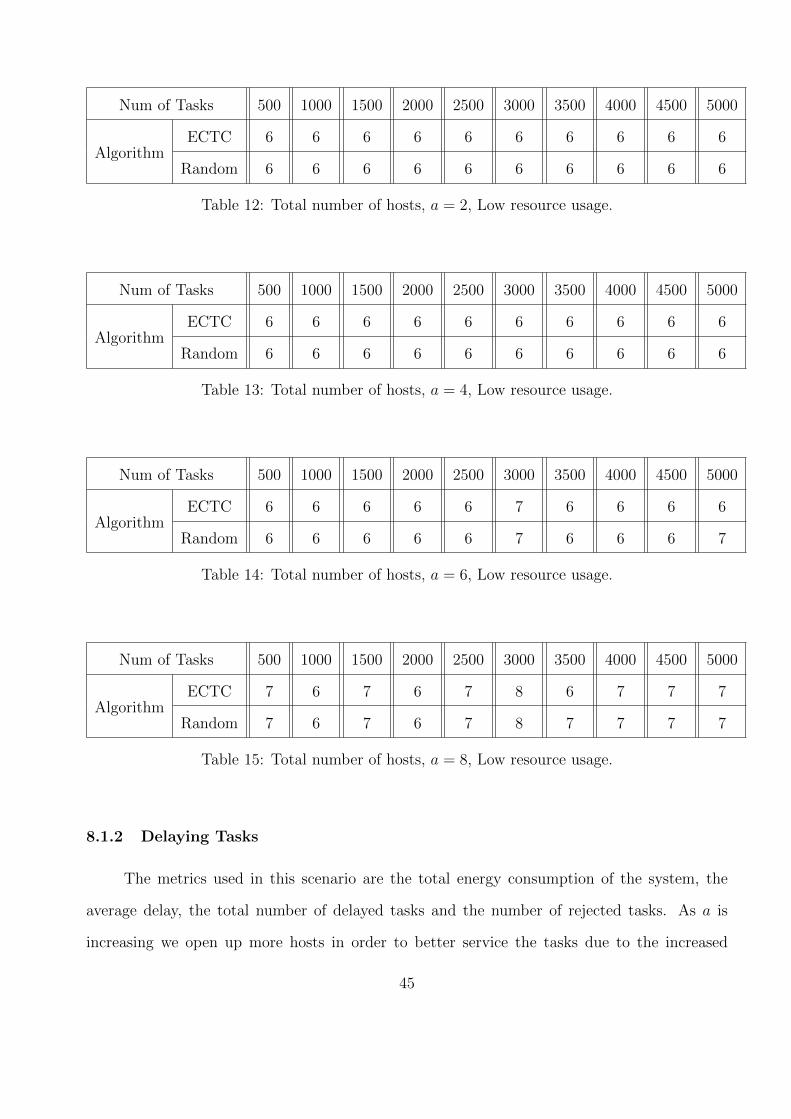
Num of Tasks 500 1000 1500 2000 2500 3000 3500 4000 4500 5000
AlgorithmECTC 6 6 6 6 6 6 6 6 6 6
Random 6 6 6 6 6 6 6 6 6 6
Table 12: Total number of hosts, a = 2, Low resource usage.
Num of Tasks 500 1000 1500 2000 2500 3000 3500 4000 4500 5000
AlgorithmECTC 6 6 6 6 6 6 6 6 6 6
Random 6 6 6 6 6 6 6 6 6 6
Table 13: Total number of hosts, a = 4, Low resource usage.
Num of Tasks 500 1000 1500 2000 2500 3000 3500 4000 4500 5000
AlgorithmECTC 6 6 6 6 6 7 6 6 6 6
Random 6 6 6 6 6 7 6 6 6 7
Table 14: Total number of hosts, a = 6, Low resource usage.
Num of Tasks 500 1000 1500 2000 2500 3000 3500 4000 4500 5000
AlgorithmECTC 7 6 7 6 7 8 6 7 7 7
Random 7 6 7 6 7 8 7 7 7 7
Table 15: Total number of hosts, a = 8, Low resource usage.
8.1.2 Delaying Tasks
The metrics used in this scenario are the total energy consumption of the system, the
average delay, the total number of delayed tasks and the number of rejected tasks. As a is
increasing we open up more hosts in order to better service the tasks due to the increased
45
system load. The values of all three metrics shown in Tables 16 - 25 represent the average over
10 experiments (10 volumes of tasks).
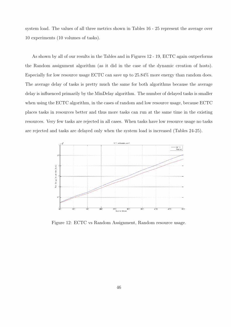
As shown by all of our results in the Tables and in Figures 12 - 19, ECTC again outperforms
the Random assignment algorithm (as it did in the case of the dynamic creation of hosts).
Especially for low resource usage ECTC can save up to 25.84% more energy than random does.
The average delay of tasks is pretty much the same for both algorithms because the average
delay is influenced primarily by the MinDelay algorithm. The number of delayed tasks is smaller
when using the ECTC algorithm, in the cases of random and low resource usage, because ECTC
places tasks in resources better and thus more tasks can run at the same time in the existing
resources. Very few tasks are rejected in all cases. When tasks have low resource usage no tasks
are rejected and tasks are delayed only when the system load is increased (Tables 24-25).
Figure 12: ECTC vs Random Assignment, Random resource usage.
46
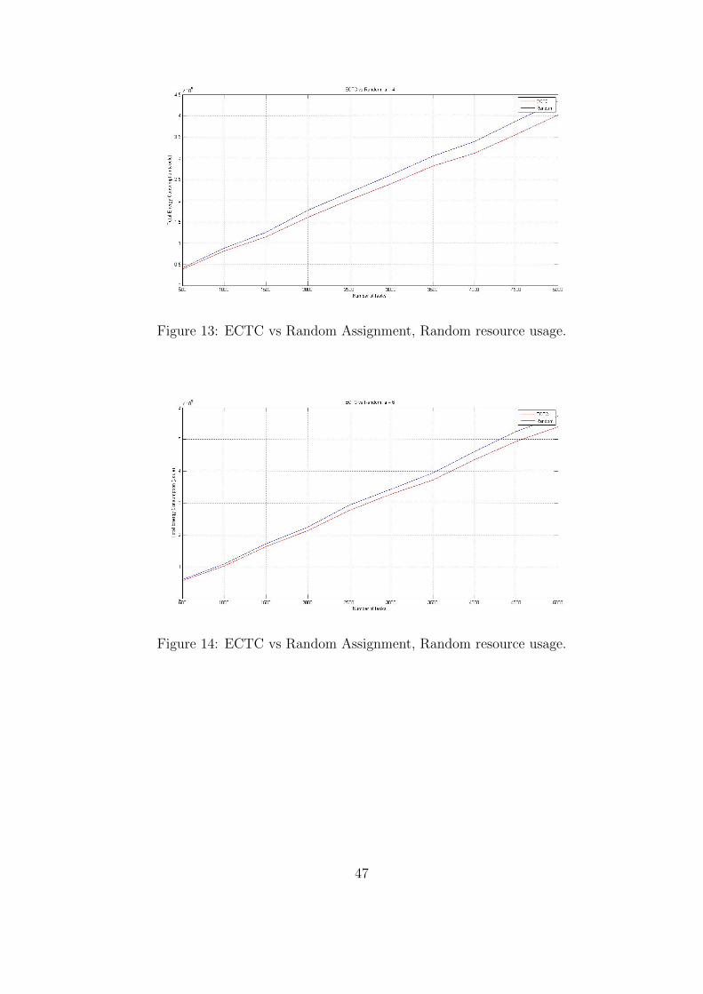
Figure 13: ECTC vs Random Assignment, Random resource usage.
Figure 14: ECTC vs Random Assignment, Random resource usage.
47
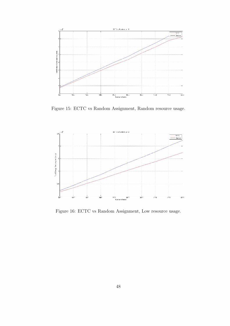
Figure 15: ECTC vs Random Assignment, Random resource usage.
Figure 16: ECTC vs Random Assignment, Low resource usage.
48

Figure 17: ECTC vs Random Assignment, Low resource usage.
Figure 18: ECTC vs Random Assignment, Low resource usage.
49

Figure 19: ECTC vs Random Assignment, Low resource usage.
a 2 4 6 8
difference 8.31% 8.15% 5.55% 8.15%
Table 16: Difference in Energy Consumption between ECTC and Random Assignment, Randomresource usage.
Metric Average Delay Delayed Tasks Rejected Tasks
AlgorithmECTC 181.2 3.2 0
Random 180.1 5.1 0
Table 17: Metric values, a = 2, Random resource usage.
Metric Average Delay Delayed Tasks Rejected Tasks
AlgorithmECTC 486.6 77.3 0
Random 473.4 99.8 0.5
Table 18: Metric values, a = 4, Random resource usage.
50

Metric Average Delay Delayed Tasks Rejected Tasks
AlgorithmECTC 877 381.2 1.6
Random 917.3 403.4 2.4
Table 19: Metric values, a = 6, Random resource usage.
Metric Average Delay Delayed Tasks Rejected Tasks
AlgorithmECTC 988.9 116.5 0
Random 1065.6 155.7 0.2
Table 20: Metric values, a = 8, Random resource usage.
a 2 4 6 8
difference 21.88% 24.8% 22.64% 19.17%
Table 21: Difference in Energy Consumption between ECTC and Random, Low resource usage.
Metric Average Delay Delayed Tasks Rejected Tasks
AlgorithmECTC 0 0 0
Random 0 0 0
Table 22: Metric values, a = 2, Low resource usage.
Metric Average Delay Delayed Tasks Rejected Tasks
AlgorithmECTC 0 0 0
Random 0 0 0
Table 23: Metric values, a = 4, Low resource usage.
51

Metric Average Delay Delayed Tasks Rejected Tasks
AlgorithmECTC 36 0.2 0
Random 77.2 0.3 0
Table 24: Metric values, a = 6, Low resource usage.
Metric Average Delay Delayed Tasks Rejected Tasks
AlgorithmECTC 79 116.5 0
Random 1065.6 223.3 0
Table 25: Metric values, a = 8, Low resource usage.
8.2 Activate Migrations vs Deactivate Migrations
In this scenario we compare the system when migrations are activated and when they are
deactivated. As we did in the previous scenario, we evaluate the system when the first option
(dynamic creation of new hosts) and when the second option (delaying tasks) is implemented,
under different system loads.
8.2.1 Dynamic creation of hosts
The metrics used in this scenario are the total energy consumption of the system and the
total number of hosts. Our results are presented in Tables 26 - 35 and Figures 20 - 27.
When the option of creating new hosts is activated, the energy consumption of the system
increases. This happens because the newly created hosts might be of no use after a time
period, but they are still drawing energy. As we can see from table 26, migrations can achieve
an improvement up to 4.17% in energy consumption. The maximum improvement in energy
consumption due to migrations is 6% in random resource usage and 7% in low resource usage.
52

This improvement can be further increased if resources that are not used for a certain period
of time are switched off (this, however, was not implemented in our system; it is left as future
work). When migrations are active, resources are used more efficiently and this can be seen in
tables 28-30; less hosts are created and thus less energy is spent. Nevertheless, in both cases
hosts will be created when tasks do not “fit” in the system and might be of no use after a time
period. In cases of low resource usage, migrations can perform better due to the fact that more
tasks can “fit” in a host; thus, by moving more VMs to other hosts energy consumption can be
decreased. As we can see from Tables 32 - 35 in some cases, when migrations are active, more
hosts are created. Still as shown in Figures 24 - 27, the activation of VM migrations always
leads to smaller energy consumption.
Figure 20: Migrations vs ECTC, Random resource usage.
53
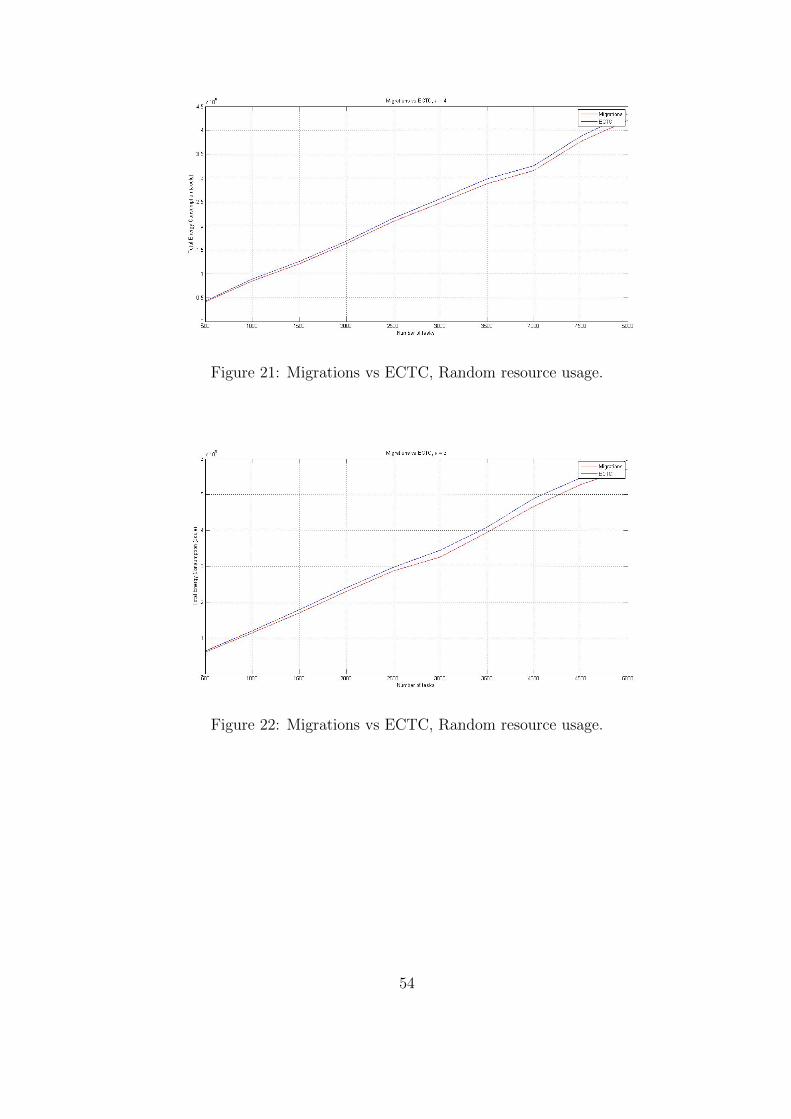
Figure 21: Migrations vs ECTC, Random resource usage.
Figure 22: Migrations vs ECTC, Random resource usage.
54

Figure 23: Migrations vs ECTC, Random resource usage.
Figure 24: Migrations vs ECTC, Low resource usage.
55
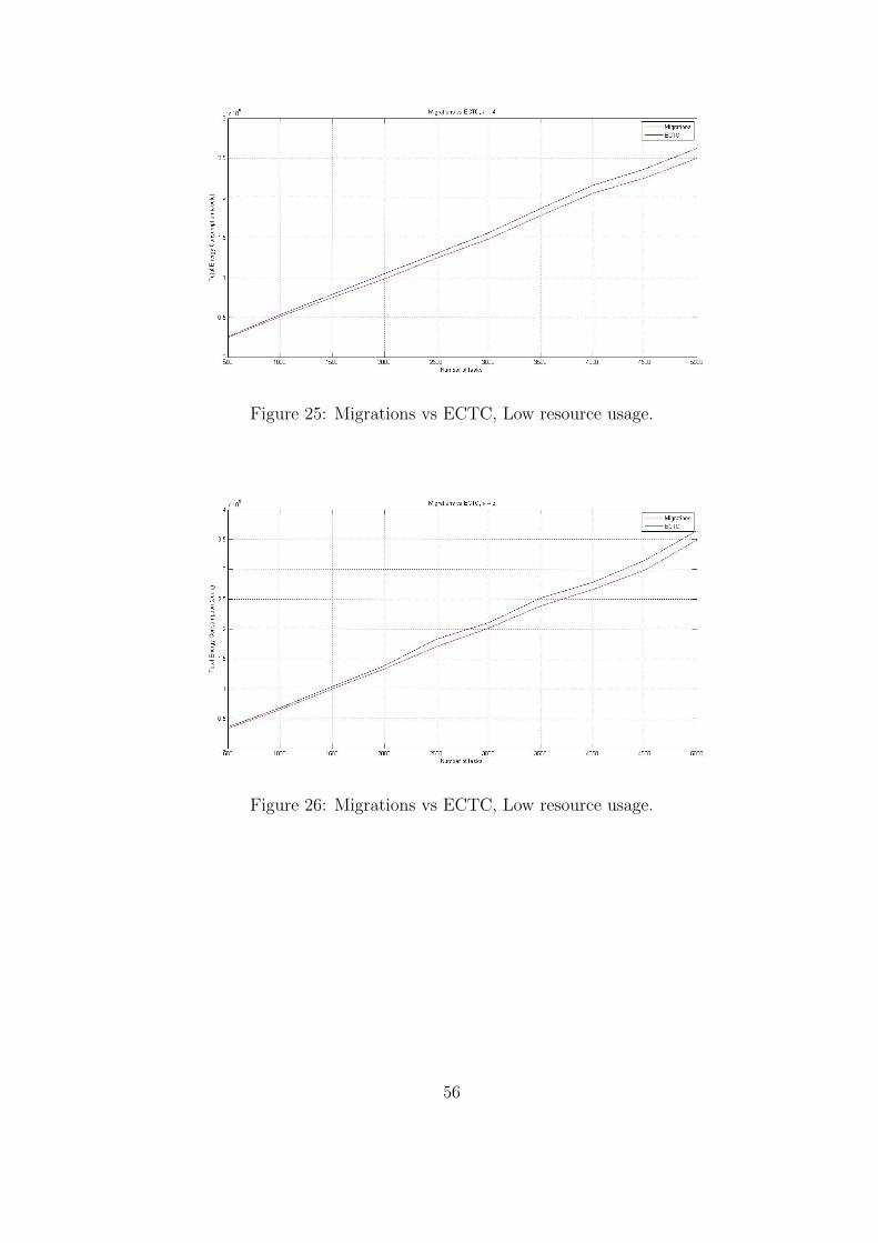
Figure 25: Migrations vs ECTC, Low resource usage.
Figure 26: Migrations vs ECTC, Low resource usage.
56

Figure 27: Migrations vs ECTC, Low resource usage.
a 2 4 6 8
difference 1.74% 3.3% 4.17% 4.14%
Table 26: Difference in Energy Consumption between ECTC with Migration and ECTC, Ran-dom resource usage.
Num of Tasks 500 1000 1500 2000 2500 3000 3500 4000 4500 5000
MigrationsYes 6 8 6 7 7 7 8 7 8 7
No 6 8 6 7 7 7 8 7 8 7
Table 27: Total number of hosts, a = 2, Random resource usage.
Num of Tasks 500 1000 1500 2000 2500 3000 3500 4000 4500 5000
MigrationsYes 8 9 10 9 10 9 9 9 10 10
No 8 10 10 9 10 10 10 9 10 10
Table 28: Total number of hosts, a = 4, Random resource usage.
57

Num of Tasks 500 1000 1500 2000 2500 3000 3500 4000 4500 5000
MigrationsYes 11 12 12 11 11 10 13 13 12 11
No 12 13 13 11 11 11 13 14 12 11
Table 29: Total number of hosts, a = 6, Random resource usage.
Num of Tasks 500 1000 1500 2000 2500 3000 3500 4000 4500 5000
MigrationsYes 12 12 13 14 17 14 14 13 13 15
No 13 13 14 15 17 14 15 13 14 15
Table 30: Total number of hosts, a = 8, Random resource usage.
a 2 4 6 8
difference 3.59% 4.95% 4.77% 3.65%
Table 31: Difference in Energy Consumption between ECTC with Migration and ECTC, Lowresource usage.
Num of Tasks 500 1000 1500 2000 2500 3000 3500 4000 4500 5000
MigrationsYes 6 6 6 6 6 6 6 6 6 6
No 6 6 6 6 6 6 6 6 6 6
Table 32: Total number of hosts, a = 2, Low resource usage.
Num of Tasks 500 1000 1500 2000 2500 3000 3500 4000 4500 5000
MigrationsYes 6 6 6 6 6 6 6 6 6 6
No 6 6 6 6 6 6 6 6 6 6
Table 33: Total number of hosts, a = 4, Low resource usage.
58
Num of Tasks 500 1000 1500 2000 2500 3000 3500 4000 4500 5000
MigrationsYes 6 6 6 6 7 6 7 6 6 7
No 6 6 6 6 6 7 6 6 6 6
Table 34: Total number of hosts, a = 6, Low resource usage.
Num of Tasks 500 1000 1500 2000 2500 3000 3500 4000 4500 5000
MigrationsYes 6 7 7 7 7 7 8 7 8 8
No 6 7 6 8 7 6 7 7 7 7
Table 35: Total number of hosts, a = 8, Low resource usage.
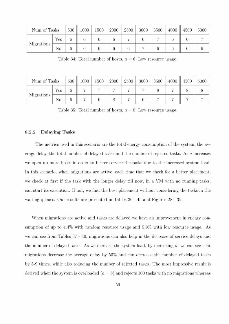
8.2.2 Delaying Tasks
The metrics used in this scenario are the total energy consumption of the system, the av-
erage delay, the total number of delayed tasks and the number of rejected tasks. As a increases
we open up more hosts in order to better service the tasks due to the increased system load.
In this scenario, when migrations are active, each time that we check for a better placement,
we check at first if the task with the longer delay till now, in a VM with no running tasks,
can start its execution. If not, we find the best placement without considering the tasks in the
waiting queues. Our results are presented in Tables 36 - 45 and Figures 28 - 35.
When migrations are active and tasks are delayed we have an improvement in energy con-
sumption of up to 4.4% with random resource usage and 5.9% with low resource usage. As
we can see from Tables 37 - 40, migrations can also help in the decrease of service delays and
the number of delayed tasks. As we increase the system load, by increasing a, we can see that
migrations decrease the average delay by 50% and can decrease the number of delayed tasks
by 5-9 times, while also reducing the number of rejected tasks. The most impressive result is
derived when the system is overloaded (a = 8) and rejects 100 tasks with no migrations whereas
59

with migrations this number drops to 5. When the task resource usage is low very few tasks
are delayed and only for a = 8.
Figure 28: Migrations vs ECTC, Random resource usage.
Figure 29: Migrations vs ECTC, Random resource usage.
60

Figure 30: Migrations vs ECTC, Random resource usage.
Figure 31: Migrations vs ECTC, Random resource usage.
61
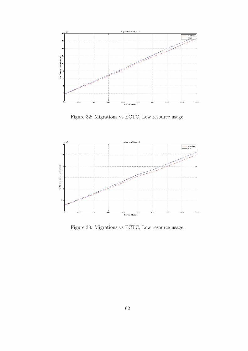
Figure 32: Migrations vs ECTC, Low resource usage.
Figure 33: Migrations vs ECTC, Low resource usage.
62

Figure 34: Migrations vs ECTC, Low resource usage.
Figure 35: Migrations vs ECTC, Low resource usage.
a 2 4 6 8
difference 1.23% 3.34% 3.29% 1.23%
Table 36: Difference in Energy Consumption between ECTC with Migration and ECTC, Ran-dom resource usage.
63

Metric Average Delay Delayed Tasks Rejected Tasks
MigrationsYes 139.3 1.5 0
No 192.9 1.9 0
Table 37: Metric values, a = 2, Random resource usage.
Metric Average Delay Delayed Tasks Rejected Tasks
MigrationsYes 564.1 230 3
No 631.6 362.8 4.8
Table 38: Metric values, a = 4, Random resource usage.
Metric Average Delay Delayed Tasks Rejected Tasks
MigrationsYes 529 41 1
No 948 355.2 1.22
Table 39: Metric values, a = 6, Random resource usage.
Metric Average Delay Delayed Tasks Rejected Tasks
MigrationsYes 812.2 212.2 4.8
No 1851.3 1081.9 100.1
Table 40: Metric values, a = 8, Random resource usage.
a 2 4 6 8
difference 3.78% 4.79% 4.4% 4.36%
Table 41: Difference in Energy Consumption between ECTC with Migration and ECTC, Lowresource usage.
64

Metric Average Delay Delayed Tasks Rejected Tasks
MigrationsYes 0 0 0
No 0 0 0
Table 42: Metric values, a = 2, Low resource usage.
Metric Average Delay Delayed Tasks Rejected Tasks
MigrationsYes 0 0 0
No 0 0 0
Table 43: Metric values, a = 4, Low resource usage.
Metric Average Delay Delayed Tasks Rejected Tasks
MigrationsYes 0 0 0
No 0 0 0
Table 44: Metric values, a = 6, Low resource usage.
Metric Average Delay Delayed Tasks Rejected Tasks
MigrationsYes 143.5 4.22 0
No 218 7.5 0
Table 45: Metric values, a = 8, Low resource usage.
65

9 Conclusions
In this thesis we implemented an energy conscious algorithm (ECTC) from the literature
in order to minimize energy consumption in cloud computing architectures, by using task con-
solidation techniques. We tried to improve the performance of our system through simulated
annealing but there was not much improvement in terms of energy consumption. We then ap-
plied the VM live migration process and we incorporated a profit driven scheduling algorithm
in our system in order to minimize the service delays.
We simulated a significant number of scenarios under different system loads in order to study
how much the energy efficiency of the system can improve with the modifications we have imple-
mented on ECTC. Our results have shown that energy consumption and delays (corresponding
to profit loss) can be simultaneously decreased with the use of an efficient scheduling algorithm.
Our future work will focus on the proposal of a scheduling algorithm that can provide even
larger gains in energy consumption, even for a high resource usage.
66

References
[1] M. Armbrust, A. Fox, R. Griffith, A. D. Joseph, R. H. Katz, A. Konwinski, G. Lee, D. A.
Patterson, A. Rabkin, I. Stoica, and M. Zaharia, Security guidance for critical areas of focus
in cloud computing v2.1, University of California, Berkeley, Tech. Rep. UCB-EECS-2009-28,
Feb 2009.
[2] Cloud Security Alliance (CSA), Security guidance for critical areas of focus in cloud com-
puting v2.1, http://www.cloudsecurityalliance.org/guidance/csaguide.v2.1.pdf.
[3] Mell, P., Grance, T., The NIST definition of cloud computing v1.5, http://www.
cloudsecurityalliance.org/guidance/csaguide.v2.1.pdf.
[4] http://www.infoworld.com/d/cloud-computing/what-cloud-computing-really-means-031.
[5] Ken E. Stavinoha, What is Cloud Computing and Why Do We Need It? http://
isacahouston.org/documents/WhatisCloudComputingandWhyDoWeNeedIt.pdf.
[6] http://cloudcomplete.blogspot.gr/2009/08/cloud-computing-why-do-we-need-it.
html.
[7] http://technet.microsoft.com/en-us/magazine/hh509051.aspx.
[8] http://info.apps.gov/content/what-are-deployment-models.
[9] http://www.south.cattelecom.com/Technologies/CloudComputing/0071626948_
chap01.pdf.
[10] ASHRAE Technical Committee, Datacom equipment power trends and cooling applications,
2005, http://books.google.gr/books/about/Datacom_Equipment_Power_Trends_and_
Cooli.html?id=pwXuAQAACAAJ&redir_esc=y.
[11] Belady C, In the data center, power and cooling costs more than the it equipment it sup-
ports, 2005. http://www.electronics-cooling.com/articles/2007/feb/a3/.
67

[12] http://searchstorage.techtarget.com.au.
[13] Y. Lee, A. Zomaya, Energy efficient utilization of resources in cloud computing systems,Vol.
60, No. 2, pp. 268-280,. The Journal of Supercomputing 113, doi:10.1007/s11227-010-0421-
3,2012.
[14] Rodrigo N. Calheiros, Rajiv Ranjan, Anton Beloglazov, Cesar A. F. De Rose, and Ra-
jkumar Buyya, CloudSim: A Toolkit for Modeling and Simulation of Cloud Computing
Environments and Evaluation of Resource Provisioning Algorithms, Software: Practice and
Experience (SPE), Volume 41, Number 1, Pages: 23-50, ISSN: 0038-0644, Wiley Press, New
York, USA, January, 2011.
[15] Fan X, Weber X-D, Barroso, Power provisioning for a warehouse-sized computer, Proc
34th annual international symposium on computer architecture (ISCA 07), 2007, pp 1323,
LA 2007.
[16] Srikantaiah S, Kansal A, Zhao F, Energy aware consolidation for cloud computing, in
Proceedings of the ACM HotPower, 2008.
[17] Meisner D, Gold BT, Wenisch TF, PowerNap: eliminating server idle power, Proc 14th
international conference on architectural support for programming languages and operating
systems (ASPLOS 09), 2009, pp 205216.
[18] Kirkpatrick, S., Gelett, C.D. and Vecchi, M.P., Optimization by simulated annealing, Sci-
ence, Vol. 220, 1983, p 671 - 680.
[19] K. Boloor, R. Chirkova, T. J. Salo, and Y. Viniotis, Heuristic-based request scheduling
subject to a percentile response time sla in a distributed cloud, in Proceedings of the IEEE
GLOBECOM, 2010.
[20] C. Clark, K. Fraser, S. Hand, J. G. Hansen, E. Jul, C. Limpach, I. Pratt, and A. Warfield,
Live migration of virtual machines, Proc. NSDI ’05, May 2005.
68
[21] A. Beloglazov and R. Buyya, Optimal online deterministic algorithms and adaptive heuris
tics for energy and performance efficient dynamic consolidation of virtual machines in cloud
data centers, Concurrency and Computation: Practice and Experience (CCPE), 2012, DOI:
10.1002/cpe.1867.
[22] A. Beloglazov, J. Abawajy, R. Buyya, Energy-aware resource allocation heuristics for effi
cient management of data centers for cloud computing, Future Generation Computer Sys-
tems, 28 (5) (2012), pp. 755768
[23] Koutsandria, G. , Investigation of Resource Allocation and Bandwidth Pricing for Cloud
Computing Architectures, Undergraduate thesis, Technical University of Crete, Chania,
Greece, 2012.
69