energies

Article

Energy-Efficient Torque Distribution Optimizationfor an Omnidirectional Mobile Robot with PoweredCaster Wheels

Wenji Jia 1,2, Guilin Yang 2,*, Chongchong Wang 2, Chi Zhang 2, Chinyin Chen 2 andZaojun Fang 2

1 College of Materials Sciences and Opto-Electronic Technology, University of Chinese Academy of Sciences,Beijing 100049, China; jiawenji@nimte.ac.cn

2 Zhejiang Key Laboratory of Robotics and Intelligent Manufacturing Equipment Technology, NingboInstitute of Materials Technology and Engineering, Chinese Academy of Sciences, Ningbo 315201, China;wangchongchong@nimte.ac.cn (C.W.); zhangchi@nimte.ac.cn (C.Z.); chenchinyin@nimte.ac.cn (C.C.);fangzaojun@nimte.ac.cn (Z.F.)

* Correspondence: glyang@nimte.ac.cn; Tel.: +86-0574-8760-4980

Received: 18 October 2019; Accepted: 19 November 2019; Published: 21 November 2019 �����������������

Abstract: A mobile robot with no less than two powered caster wheels (PCWs) has the ability toperform omnidirectional motions and belongs to a redundantly actuated system. Redundant actuationwill bring the issue of non-uniqueness of actuating torque distribution, and inappropriate choicesof torque distribution schemes will lead to unexpected large required actuating torques and extraenergy consumption. This paper proposes a new torque distribution optimization approach based ona gradient projection method (GPM) for the omnidirectional mobile robot (OMR) with direct drivePCWs. It can significantly reduce the maximal required actuating torque and the energy consumptionof the system. The modular kinematic and dynamic modeling method is presented first, which issuitable for an arbitrary number of employed PCWs, as well as their install positions in the chassis.The detailed energy consumption model of the OMR, including output energy consumption andelectrical energy loss, is formulated through experimental testing. The effectiveness of the proposedalgorithms is validated by simulation examples. Lastly, the computational efficiency of the methodis verified.

Keywords: omnidirectional mobile robot; torque distribution; mobile; energy consumption model

1. Introduction

Omnidirectional mobile robots (OMRs) are widely employed to perform tasks in narrow andcongested space for their ability to instantaneously move in any direction regardless of the currentposes. Among a variety of categories of OMRs, the mobile robot with powered castor wheels (PCWs)has a simple and efficient wheel design to achieve omnidirectional motions [1]. It can carry a heavypayload and is less sensitive to the ground conditions owing to the continuous contact between thewheels and the ground [2]. For fully utilizing their maneuverability and agility, OMRs are powered byonboard batteries. Energy-efficient becomes a vital performance index for OMRs as they are usuallyrestricted by the heavy and expensive batteries [3].

It is of great significance to study the energy consumption of the mobile robots, and energy-savingstrategies have been conducted by many researchers via different aspects, for example, trajectoryplanning [4–6], motion control [7,8], and mechanical design [9]. In order to study the energy-efficientstrategies, a detailed and accurate energy consumption model needs to first be established for therobot system. Hou et al. [10] propose an energy consumption model that incorporates three major

Energies 2019, 12, 4417; doi:10.3390/en12234417 www.mdpi.com/journal/energies

Energies 2019, 12, 4417 2 of 19

components: the sensor system, control system, and motion system. It is clarified by experimentsthat the motion system part consumes the overwhelming majority of energy, with up to more than90%. Xu et al. [11] present an energy consumption modelling method for an industry robot. Theirmethod does not have to measure the relevant parameters inside the robot and mainly concerns torquemodelling. A parameter estimation method is proposed for the torque modelling. Verstraten et al. [12]study several modeling methods that are commonly adopted. They investigate how well these methodscan be used to describe the energy consumption of a DC motor while performing dynamic tasks.The conclusion resulted from their work provides guidelines in determining which factors should beincluded in the energy consumption model. In this paper, we aim to study the impacts of differenttorque distribution schemes on the energy consumption of the OMR with PCWs. Hence, we focuson formulating the energy consumption model based on the actuation torques. Besides theoreticalenergy consumption modelling, the accurate experimental measurement of energy consumption isnecessary for the evaluation of energy consumption of a system combined with hardware and software.Laopoulos et al. [13] present a current measurement method that monitors the instantaneous supplycurrent. The method can provide high-performance evaluation of energy consumption, especially forlow-power applications. Roennau et al. [14] propose an energy consumption estimation based on anon-board current measurement for each joint individually and employ a non-linear function to fit themeasurement. There are two different motors integrated in a single PCW, which are responsible forrolling and steering motions, respectively. The energy consumption modelling methods for the twomotors are unified; detailed specifications of the energy consumption models can be obtained throughseparate energy consumption measurements.

The OMR with PCWs can be considered as a redundantly actuated parallel robot system. Thoughits degree-of-freedom remains constant regardless of the number of PCWs engaged, the distributionscheme for actuator torques remains non-unique. To obtain the torque distribution, the robot Jacobianis widely employed. However, for the OMR with redundant PCWs, the Jacobian matrix cannotbe obtained directly in kinematics. Instead, the Jacobian matrix usually is computed through thegeneralized inverse of the constraint matrix [15]. Different methods for computing the generalizedinverse of the constraint matrix are investigated to achieve better dynamic performance. Holmberg [16]and Li [17] both employ the augmented object model (AOM) to obtain the operational space dynamicsof the OMR with PCWs. Holmberg uses the pseudoinverse to determine the Jacobian matrix forminimizing the total perceived slip in a least-squares manner, and Li uses another pseudoinversefor minimizing the joint velocity differences, also in a least-squares manner. With these torquedistribution schemes, the performances of slip-minimization and stability are improved to someextent. However, the strategy of choosing the torque distribution scheme is simply based on theMoore–Penrose pseudoinverse calculation, and it is difficult to further study its influence on dynamicperformances, for example, the actuating torque limits and the energy efficiency. Liu et al. [18] present acontroller for torque distribution of an OMR by identification of the status of the vehicle and the wheelslip ratio. Zhao et al. [19] present an integrated scheme for motion control and internal force control foran OMR with PCWs. The controller for the torque distribution minimizes the internal force occurringduring the robot motion. Though the torque distribution is a crucial issue for the redundantly actuatedOMR with PCWs, few studies have investigated the torque distribution optimization for minimumenergy consumption or maximal required actuating torque control.

This paper proposes a torque distribution optimization for the OMR with PCWs by using thegradient projection method (GPM). The OMR is designed in a modular way in that an arbitrary numberof PCWs can be installed in any position of the OMR’s chassis. Modular kinematic and dynamicmodelling methods are proposed. An energy consumption model is then presented to predict theenergy consumed by the motion of the OMR and the concurrent electrical loss; the coefficients of themodel are obtained from the experimental test. In the optimization algorithm, a performance criterioncombined with torque limits and energy consumption is proposed. The vital target of the OMRperformance indexes including energy endurance and tracking precision are successfully optimized by

Energies 2019, 12, 4417 3 of 19

the proposed algorithm. Finally, the computational efficiency of the optimization method is verifiedthrough simulation examples.

2. Design and Modelling of the OMR

The PCWs for the OMR are designed as a direct driving type. Two direct driving motors areintegrated in a PCW, as shown in Figure 1. The upper motor is responsible for the steering motion, andthe hub wheel motor is responsible for the rolling motion. All the PCWs are installed in the chassis ofthe OMR, the control system and other devices, such as the battery and sensors, are installed insidethe mobile platform. By virtue of the direct driving PCWs, there is no transmission mechanism in thesystem, and the efficiency and stability of motion of the OMR are improved. Moreover, the PCW isintegrated with less components, and the reliability of the direct driving PCW is also better than theconventional ones. The prototype of the OMR with two direct driving PCWs is shown in Figure 2.

Energies 2019, 12, x FOR PEER REVIEW 3 of 21

2. Design and Modelling of the OMR

The PCWs for the OMR are designed as a direct driving type. Two direct driving motors are integrated in a PCW, as shown in Figure 1. The upper motor is responsible for the steering motion, and the hub wheel motor is responsible for the rolling motion. All the PCWs are installed in the chassis of the OMR, the control system and other devices, such as the battery and sensors, are installed inside the mobile platform. By virtue of the direct driving PCWs, there is no transmission mechanism in the system, and the efficiency and stability of motion of the OMR are improved. Moreover, the PCW is integrated with less components, and the reliability of the direct driving PCW is also better than the conventional ones. The prototype of the OMR with two direct driving PCWs is shown in Figure 2.

(a) (b)

Figure 1. The designed direct driving powered caster wheel (PCW). (a) Schematic figure of the PCW; (b) prototype of the PCW.

Figure 2. Prototype of the omnidirectional mobile robot (OMR) with PCWs.

2.1. Kinematic Model of the OMR

The kinematic analysis of the OMR with PCWs will be presented in this section. Because the OMR moves on a horizontal surface, its motion can be described in a 2D frame. The OMR is designed in a modular pattern, which means we can choose the appropriate number of PCWs as well as their installing positions according to specific task requirements. A schematic diagram that illustrates the kinematic model of that modular designed OMR is presented in Figure 3. We assume that there are n-PCWs installed in the chassis of the OMR, and the points ( )i 1, 2, ,iA n= represent the install positions for the PCWs, which are also called support points. The support points can also be regarded as the distal ends of the PCWs. A PCW is actuated by two active joints, which are responsible for the rolling motion and steering motion, respectively. It can produce a driving wrench

( ) ( ), , i 1, 2, ,i i i

Twi x y zF f f m n= = to the support point in the platform. The resultant forces by all

PCWs will drive the OMR to perform the desired trajectory.

Figure 1. The designed direct driving powered caster wheel (PCW). (a) Schematic figure of the PCW;(b) prototype of the PCW.

Energies 2019, 12, x FOR PEER REVIEW 3 of 21

2. Design and Modelling of the OMR

The PCWs for the OMR are designed as a direct driving type. Two direct driving motors are integrated in a PCW, as shown in Figure 1. The upper motor is responsible for the steering motion, and the hub wheel motor is responsible for the rolling motion. All the PCWs are installed in the chassis of the OMR, the control system and other devices, such as the battery and sensors, are installed inside the mobile platform. By virtue of the direct driving PCWs, there is no transmission mechanism in the system, and the efficiency and stability of motion of the OMR are improved. Moreover, the PCW is integrated with less components, and the reliability of the direct driving PCW is also better than the conventional ones. The prototype of the OMR with two direct driving PCWs is shown in Figure 2.

(a) (b)

Figure 1. The designed direct driving powered caster wheel (PCW). (a) Schematic figure of the PCW; (b) prototype of the PCW.

Figure 2. Prototype of the omnidirectional mobile robot (OMR) with PCWs.

2.1. Kinematic Model of the OMR

The kinematic analysis of the OMR with PCWs will be presented in this section. Because the OMR moves on a horizontal surface, its motion can be described in a 2D frame. The OMR is designed in a modular pattern, which means we can choose the appropriate number of PCWs as well as their installing positions according to specific task requirements. A schematic diagram that illustrates the kinematic model of that modular designed OMR is presented in Figure 3. We assume that there are n-PCWs installed in the chassis of the OMR, and the points ( )i 1, 2, ,iA n= represent the install positions for the PCWs, which are also called support points. The support points can also be regarded as the distal ends of the PCWs. A PCW is actuated by two active joints, which are responsible for the rolling motion and steering motion, respectively. It can produce a driving wrench

( ) ( ), , i 1, 2, ,i i i

Twi x y zF f f m n= = to the support point in the platform. The resultant forces by all

PCWs will drive the OMR to perform the desired trajectory.

Figure 2. Prototype of the omnidirectional mobile robot (OMR) with PCWs.

2.1. Kinematic Model of the OMR

The kinematic analysis of the OMR with PCWs will be presented in this section. Because the OMRmoves on a horizontal surface, its motion can be described in a 2D frame. The OMR is designed in amodular pattern, which means we can choose the appropriate number of PCWs as well as their installingpositions according to specific task requirements. A schematic diagram that illustrates the kinematicmodel of that modular designed OMR is presented in Figure 3. We assume that there are n-PCWsinstalled in the chassis of the OMR, and the points Ai(i = 1, 2, · · · , n) represent the install positions forthe PCWs, which are also called support points. The support points can also be regarded as the distalends of the PCWs. A PCW is actuated by two active joints, which are responsible for the rolling motion

and steering motion, respectively. It can produce a driving wrench Fwi =

(fxi , fyi , mzi

)T(i = 1, 2, · · · , n)

Energies 2019, 12, 4417 4 of 19

to the support point in the platform. The resultant forces by all PCWs will drive the OMR to performthe desired trajectory.Energies 2019, 12, x FOR PEER REVIEW 4 of 21

Figure 3. Modular design of the OMR with n PCWs.

The global reference frame XYZ is used to describe the configuration of the OMR, and , ,i j k

represent the three orthogonal axes of the local frame attached to the platform. As long as the number of PCWs is no less than two for singularity avoidance [20], the proposed kinematic analysis for the modular OMR is not restricted by the number of PCWs. Conventionally, the PCWs are arranged symmetrically for good dynamic performance and increasing the number of PCWs can improve the load capacity of the OMR. It should be noted that the kinematic model in this paper refers to the instantaneous kinematics, which maps the joint velocity q to the operational space velocity x . As

shown in Figure 3, ( )i 1, 2, ,i nρ = are defined as the rolling angles of the wheels and ij are defined as the steering angles; iσ are defined as the angular displacements of the ith wheels with respect to the X-axis. r denotes the wheels’ radius and b denotes the offset of the PCW, l is the vector

for the center of the OMR to the support point, and α is the angle between l and i

. Then for the ith PCW, the linear speed at the center of the platform can be derived by

(sin cos )

(- cos sin )

( sin cos )

iC O i i i

i i i

i i

i i

r

b b h

l l

s wr j js j jw a a

= + ´ + ´

= + ´+ ´ + ++ ´ +

v v k O A k A Ci j k

k i j kk i j

. (1)

Note that ω , representing the angular velocity of the OMR, can be computed by

w s j= + . (2)

Combining (1) and (2), the kinematics of a PCW can be expressed in a single matrix form written as

- sin sin cos sin

cos cos sin cos

1 0 1

x i i i i i

y i i i i i

i

v b l r l

v b l r l

j a j a sj a j a r

w j

é ù é ù é ù- -ê ú ê ú ê úê ú ê ú ê ú= +ê ú ê ú ê úê ú ê ú ê úê ú ê ú ê úë û ë û ë û

. (3)

Equation (3) presents the forward kinematic model of wheel i and the kinematic models of the rest of the wheels can be derived in the same manner. The single castor wheel Jacobian matrix iJ is always full rank as its determinant remains a nonzero constant. Thus, the inverse matrix of iJ always exists.

In practice, it would be difficult to measure or control iσ as it represents a passive rotational motion. This variable needs to be eliminated from the inverse kinematics of a single PCW. The

Figure 3. Modular design of the OMR with n PCWs.

The global reference frame XYZ is used to describe the configuration of the OMR, and→

i ,→

j ,→

krepresent the three orthogonal axes of the local frame attached to the platform. As long as the numberof PCWs is no less than two for singularity avoidance [20], the proposed kinematic analysis for themodular OMR is not restricted by the number of PCWs. Conventionally, the PCWs are arrangedsymmetrically for good dynamic performance and increasing the number of PCWs can improve theload capacity of the OMR. It should be noted that the kinematic model in this paper refers to theinstantaneous kinematics, which maps the joint velocity

.q to the operational space velocity

.x. As shown

in Figure 3, ρi(i = 1, 2, · · · , n) are defined as the rolling angles of the wheels and ϕi are defined as thesteering angles; σi are defined as the angular displacements of the ith wheels with respect to the X-axis.r denotes the wheels’ radius and b denotes the offset of the PCW, l is the vector for the center of the

OMR to the support point, and α is the angle between l and→

i . Then for the ith PCW, the linear speedat the center of the platform can be derived by

vC = vOi +.σk×OiAi +ωk×AiC

=.ρi(sinϕii + cosϕij) × rk

+.σk× (−b cosϕii + b sinϕij + hk)+ωk× (l sinαii + l cosαij)

. (1)

Note that ω, representing the angular velocity of the OMR, can be computed by

ω =.σ+

.ϕ. (2)

Combining (1) and (2), the kinematics of a PCW can be expressed in a single matrix form written asvx

vy

ω

=−b sinϕi − l sinαi r cosϕi −l sinαib cosϕi + l cosαi r sinϕi l cosαi

1 0 1

.σi.ρi.ϕi

. (3)

Equation (3) presents the forward kinematic model of wheel i and the kinematic models of the restof the wheels can be derived in the same manner. The single castor wheel Jacobian matrix Ji is alwaysfull rank as its determinant remains a nonzero constant. Thus, the inverse matrix of Ji always exists.

Energies 2019, 12, 4417 5 of 19

In practice, it would be difficult to measure or control σi as it represents a passive rotational motion.This variable needs to be eliminated from the inverse kinematics of a single PCW. The controllablejoint velocity denoted by qi, including steering and rolling variables only, can be expressed as

.qi =

[ .ρi.ϕi

]= Ci

vx

vy

ω

, (4)

where Ci is called the wheel constraint matrix [16] because it describes the constraints at each contactpoint between the wheel and the ground. All wheels’ equations are combined to get the unified inversekinematics, as follows:

C =

C1

C2...

Cn

,.q =

.q1.q2...

.qn

= C.x. (5)

2.2. Joint Space Dynamic Model of the OMR

In order to formulate the dynamic model of the entire system, the dynamic model of a single PCWshould first be obtained. In Figure 4, the schematic model of the PCW is presented. A PCW consists ofthree main components: a wheel, a bracket, and a “virtual” link from the upper side of the bracket tothe mass center of the OMR. We call the link “virtual” because it only exists conceptually. The PCWsare installed directly in the chassis of the robot. The virtual link just provides the position informationof the support points from the mass center of the robot.

Energies 2019, 12, x FOR PEER REVIEW 5 of 21

controllable joint velocity denoted by iq , including steering and rolling variables only, can be expressed as

=x

ii i y

i

v

q C vrj

w

é ùê úé ù ê úê ú= ê úê ú ê úê úë û ê úë û

, (4)

where iC is called the wheel constraint matrix [16] because it describes the constraints at each contact point between the wheel and the ground. All wheels’ equations are combined to get the unified inverse kinematics, as follows:

1 1

2 2,

n n

C q

C qC q Cx

C q

é ù é ùê ú ê úê ú ê úê ú ê ú= = =ê ú ê úê ú ê úê ú ê úê ú ê úë û ë û

. (5)

2.2. Joint Space Dynamic Model of the OMR

In order to formulate the dynamic model of the entire system, the dynamic model of a single PCW should first be obtained. In Figure 4, the schematic model of the PCW is presented. A PCW consists of three main components: a wheel, a bracket, and a “virtual” link from the upper side of the bracket to the mass center of the OMR. We call the link “virtual” because it only exists conceptually. The PCWs are installed directly in the chassis of the robot. The virtual link just provides the position information of the support points from the mass center of the robot.

Figure 4. Simplified PCW model subjected to driving torques.

The equation of motion for a PCW can be obtained through the Lagrangian method. The OMR can only achieve planner motion, hence there only exists kinetic energy iK . The rolling motion iρ is always orthogonal to the steering motion iϕ , thus they can be decoupled and calculated by

2 2 2( r)2 2 2r i s i w i

iI I m

Kρ ϕ ρ

= + +

, (6)

where rI is the inertial moment of the wheel about its rolling axis, sI is the inertial moment of the PCW about the steering axis, and wm is the mass of the PCW. The dynamic model of a PCW in the joint space can be derived as

i

i

i i

i i

K Kd

dt q qr

j

tt

é ù¶ ¶ ê ú- = ê ú¶ ¶ ê úë û. (7)

Because iK is only in regard to iq , / 0i iK q∂ ∂ = holds. The dynamic model of a single PCW can be formulated as

Figure 4. Simplified PCW model subjected to driving torques.

The equation of motion for a PCW can be obtained through the Lagrangian method. The OMRcan only achieve planner motion, hence there only exists kinetic energy Ki. The rolling motion

.ρi is

always orthogonal to the steering motion.ϕi, thus they can be decoupled and calculated by

Ki =Ir

.ρ

2i

2+

Is.ϕ

2i

2+

mw(.ρir)

2

2, (6)

where Ir is the inertial moment of the wheel about its rolling axis, Is is the inertial moment of the PCWabout the steering axis, and mw is the mass of the PCW. The dynamic model of a PCW in the joint spacecan be derived as

ddt∂Ki

∂.qi−∂Ki∂qi

=

[τρi

τϕi

]. (7)

Because Ki is only in regard to.qi, ∂Ki/∂qi = 0 holds. The dynamic model of a single PCW can be

formulated asMi

..qi = τi − τ fi + PT

i (−Fwi ), (8)

Energies 2019, 12, 4417 6 of 19

where

Mi =

[Ir + mr2 0

0 Is

],

..qi =

[ ..ρi..ϕi

],

PTi =

[−r cosϕi b sinϕi 0

0 0 1

].

In (8), τi represents the actuating torques and τ fi denotes the friction torques, which consist ofCoulomb friction and viscous friction. Pi is the matrix that maps the ith joint velocity to the supportpoint velocity, and −Fi is the external wrench applied by the platform.

The platform of the OMR can then be regarded as a manipulated object by the PCWs. Theforce resulted from the distal end of ith PCW is Fw

i . The dynamic model of the platform only can beexpressed as

Λp..x + µp(x,

.x) = Fw

o , (9)

where Λp = diag[

mo mo Io]

is the inertial term of the platform, and µp(x,.x) is the Coriolis and

centrifugal term. Fwo is the resultant force applied by all the PCWs.

2.3. Operational Space Dynamic Model of the OMR

The operational space dynamic model of a PCW is expressed in the form as

Λi..x + µi = Fi, (10)

where Λi = CTi MiCi is the operational space mass matrix, µi = CT

i Mi.Ci is the operational space Coriolis

and centripetal terms, and Fi is the operational space wrench. The OMR is assumed to move in a planesurface, so the gravity component is neglected here.

After deriving the dynamic models of the PCWs, the augmented object model (AOM) [21] can beemployed to obtain the dynamic model of the entire system. The AOM declares that the systematicdynamic model of the entire system in operational space can be obtained by adding all the operationalspace dynamics of the PCWs and the platform only at the operational space frame. Thus, the augmentedmass matrix Λ⊕ and Coriolis and centripetal terms µ⊕ of the OMR are given as

Λ⊕ =n∑

i=1

Λi + Λp, (11)

µ⊕ =n∑

i=1

µi + µp, (12)

where Λp and µp are the mass matrix and the Coriolis and centripetal terms of the platform onlyexpressed in the operational space, respectively. F is the resultant wrench applied to the OMR, expressedin the operational space frame. Finally, the operational dynamics of the OMR can be written as

Λ⊕..x + µ⊕ = F. (13)

3. Energy Consumption Model of the OMR

The intact energy consumption model of the OMR consists of three parts: the sensors, the controlsystem, and the motion system. The motion system consumes the overwhelming majority of energyin the OMR [10]. Hence, we mainly focus on the study of the influence of torque distributions to theenergy consumption. The energy consumptions of the sensor system and the control system will notbe discussed here. The formulation of energy consumption model is for predicting and evaluating the

Energies 2019, 12, 4417 7 of 19

amount of energy consumed by the actuators in the OMR. The energy consumption can be calculatedby integrating the power consumption about time. The power consumption model usually consist ofoutput power consumption Poutput and the subordinate electrical power loss Ploss [22,23].

Ptotal = Poutput + Ploss, (14)

where the output power consumption is the power consumed to attain and sustain the desired motionof the OMR, and refers to the mechanical power. Poutput can be computed by

Poutput =n∑

i=1

[τi

.qi

]∗. (15)

The definition of [a]∗ is that, if a is larger than zero, the value of [a]∗ is a. If a is smaller than zero, theoutcome value of the function is zero. It means that the negative output power cannot be regeneratedand is dissipated as heat [24].

The electrical power loss often contains three parts: coil loss, conduction loss, and switching loss.The coil loss results from the heat dissipation as the current flows through the resistances of a circuit. Itis formulated as follows:

Pcoil =n∑

i=1

RiI2i , (16)

where Ri is the resistance of the coil in the ith actuator. Ii is the current the of the ith actuator. The othertwo types of electrical power loss that happen in servo-amplifiers or servo-drives, including conductionloss and switching loss. Each loss happens when the current flows in an insulated-gate bipolar transistorof the servo-amplifier [25]. The conduction loss and switching loss are often formulated accordingto the voltage and current information. The literature of [25] provides a scheme for calculating theconduction and switching loss only dependent on the current information. The conduction loss andthe switch loss can be expressed, respectively, by:

Pconduction =n∑

i=1

µai Ii + µb

i I2i , (17)

Pswitching =n∑

i=1

ηiIi, (18)

where µai and µb

i are the coefficients for the conduction loss. The conduction loss is formulated in aquadratic polynomial manner with respect to the current. ηi is the constant coefficient of switchingwith respect to the current. Hence, the electrical power loss can be computed by summing the coil loss,conduction loss, and switching loss.

Ploss = Pcoil + Pconduction + Pswitching. (19)

All kinds of losses are formulated as the functions of current. By summing the coefficientsaccording to the power of the current, the power loss can be expressed as

Ploss =n∑

i=1

(λa

i Ii + λbi I2

i

), (20)

where λai = µa

i + ηi, and λbi = µb

i +Ri. λai and λb

i are the coefficients of the power loss of the ith actuatorin terms of the current.

Because we mainly investigate the relationship between the torque distributions and the energyconsumption in this paper, it is desired to express the power consumption in the manner of joint torques.

Energies 2019, 12, 4417 8 of 19

Fortunately, for the torque motors employed in the PCWs, their outputs are linearly proportional tothe current in the circuit. Therefore, the current term Ii and I2

i in (20) can be replaced by the torqueterm τi and τ2

i with their corresponding linear coefficients. Equation (20) can be reformulated as

Ploss =n∑

i=1

(κa

i |τi|+ κbi τ

2i

), (21)

where κai and κb

i are the coefficients for the electrical power loss of the absolute value of torque and thesquare of torque in the ith actuator, respectively. The new electrical power loss model (21) in terms ofthe torque represents a combination of the electrical power loss model in terms of the current and thelinear proportional relationship between the current and the torque in the actuator.

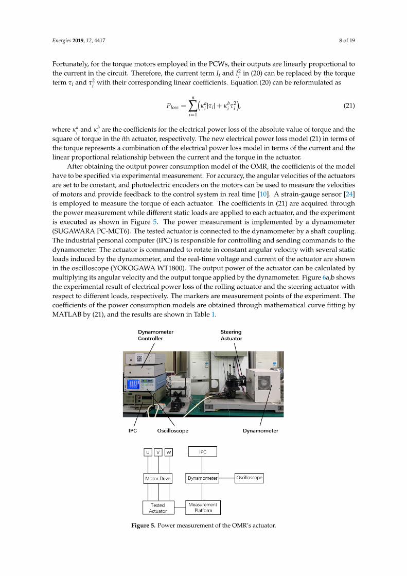
After obtaining the output power consumption model of the OMR, the coefficients of the modelhave to be specified via experimental measurement. For accuracy, the angular velocities of the actuatorsare set to be constant, and photoelectric encoders on the motors can be used to measure the velocitiesof motors and provide feedback to the control system in real time [10]. A strain-gauge sensor [24]is employed to measure the torque of each actuator. The coefficients in (21) are acquired throughthe power measurement while different static loads are applied to each actuator, and the experimentis executed as shown in Figure 5. The power measurement is implemented by a dynamometer(SUGAWARA PC-MCT6). The tested actuator is connected to the dynamometer by a shaft coupling.The industrial personal computer (IPC) is responsible for controlling and sending commands to thedynamometer. The actuator is commanded to rotate in constant angular velocity with several staticloads induced by the dynamometer, and the real-time voltage and current of the actuator are shownin the oscilloscope (YOKOGAWA WT1800). The output power of the actuator can be calculated bymultiplying its angular velocity and the output torque applied by the dynamometer. Figure 6a,b showsthe experimental result of electrical power loss of the rolling actuator and the steering actuator withrespect to different loads, respectively. The markers are measurement points of the experiment. Thecoefficients of the power consumption models are obtained through mathematical curve fitting byMATLAB by (21), and the results are shown in Table 1.Energies 2019, 12, x FOR PEER REVIEW 9 of 21

Figure 5. Power measurement of the OMR’s actuator.

Figure 5. Power measurement of the OMR’s actuator.

Energies 2019, 12, 4417 9 of 19

Energies 2019, 12, x FOR PEER REVIEW 10 of 21

(a)

(b)

Figure 6. Experimental results of the electrical power loss: (a) function fitting for the rolling motor; (b) function fitting for the steering motor.

From the above, the total power consumption of the motion system can be written as

[ ] ( )*

2

1 1

n na b

total i i i i i ii i

P qτ κ τ κ τ= =

= + + . (22)

The energy consumption model for the OMR can be calculated by

( ) [ ] ( )0

*2

1 1

ft n na b

i i i i i ii it

E qτ τ κ τ κ τ= =

= + +

. (23)

Each PCW has two motors for rolling and steering motions, respectively, so the number n is 2m for the OMR with m PCWs.

4. Torque Distribution Schemes for the OMR

The torque distribution schemes of robots can be derived from the forward kinematic model by

TJ Fτ = , (24)

where τ is the actuating torques applied by the joints and J is the Jacobian matrix of the robot. In the analysis of the torque distribution for the OMR, because the PCWs are direct driven, the impact of the transmission system in the PCWs and the dynamics of the motors are neglected. We assume that the torques produced by the actuators are the same torques applied to the joints. Owing to the parallel structure and redundant actuation of the OMR, the Jacobian matrix cannot be derived

Figure 6. Experimental results of the electrical power loss: (a) function fitting for the rolling motor; (b)function fitting for the steering motor.

Table 1. Experimental results for the coefficients of the power loss model.

Class of Actuators κai κb

i

Steering actuator 2.98 1.40Rolling actuator 3.39 2.31

From the above, the total power consumption of the motion system can be written as

Ptotal =n∑

i=1

[τi

.qi

]∗+

n∑i=1

(κa

i |τi|+ κbi τ

2i

). (22)

The energy consumption model for the OMR can be calculated by

E(τ) =

t f∫t0

n∑i=1

[τi

.qi

]∗+

n∑i=1

(κa

i |τi|+ κbi τ

2i

). (23)

Each PCW has two motors for rolling and steering motions, respectively, so the number n is 2mfor the OMR with m PCWs.

Energies 2019, 12, 4417 10 of 19

4. Torque Distribution Schemes for the OMR

The torque distribution schemes of robots can be derived from the forward kinematic model by

τ = JTF, (24)

where τ is the actuating torques applied by the joints and J is the Jacobian matrix of the robot. In theanalysis of the torque distribution for the OMR, because the PCWs are direct driven, the impact of thetransmission system in the PCWs and the dynamics of the motors are neglected. We assume that thetorques produced by the actuators are the same torques applied to the joints. Owing to the parallelstructure and redundant actuation of the OMR, the Jacobian matrix cannot be derived directly throughkinematics analysis. Instead, it is obtained by computing the generalized inverse of the constrainedmatrix C of the OMR [15]. This means that if the task space velocity of the OMR is given, the jointvelocity can be directly calculated by the constraint matrix. However, the task space velocity cannot beobtained from arbitrary joint velocity because of the kinematic constraints. The constraint matrix mapsthe operational space velocity

.x to the joint space velocity

.q by

.x = C

.q. (25)

The Jacobian matrix of the OMR can be obtained by computing the generalized inverse matrix ofthe constraint matrix:

J = C+. (26)

Because the OMR is redundantly actuated, the constraint matrix C is not square. Hence, thereexists a non-unique Jacobian matrix for the OMR, and the different choices of the generalized inversewill lead to different torque distribution schemes.

4.1. Torque Distribution Schemes Resulting from the Generalized Inverse of the Jacobian

Two reasonable determinations of torque distribution schemes proposed by the publishedresearch [17] are first presented. The kinematics of the OMR with PCWs can be expressed in anequivalent way as

A.x = B

.q, (27)

where B is a diagonal matrix and A is a non-square matrix. The first torque distribution scheme isexpressed as

τ =(B−1A

)T

LPIF, (28)

where(B−1A

)LPI

means computing the left Moore–Penrose pseudo-inverse of B−1A. Using this model,the joint torque differences are minimized in a least-squares manner. The second torque distributionscheme is expressed as

τ = BTATLPIF, (29)

where ALPI means computing the left Moore–Penrose pseudo-inverse of A. Using this model, thejoint torque as well as the interaction forces between different contact points are minimized, in aleast-squares manner.

4.2. Gradient Projection-Based Torque Optimization

The gradient projection method is an efficient and widely-employed optimization method in thecontrol of redundant robots [26,27]. It fully utilizes the null space of the Jacobian matrix to optimizevarieties of performance criteria, such as manipulability, obstacle avoidance, and joint limit avoidance.It is approached by projecting the steepest descent direction of the performance criterion onto thenull space and finding the best solution along the projected vector. The flowchart of the proposedtorque distribution optimization algorithm is shown in Figure 7. For the torque distribution of the

Energies 2019, 12, 4417 11 of 19

redundant actuated OMR, as mentioned before, the joint space torque is not directly projected from theoperational space force by the transpose of the Jacobian matrix, but instead of the constraint matrix C,written by

CTτ = F. (30)Energies 2019, 12, x FOR PEER REVIEW 12 of 21

4.2. Gradient Projection-Based Torque Optimization

Figure 7. Flowchart of the optimization algorithm.

The gradient projection method is an efficient and widely-employed optimization method in the control of redundant robots [26,27]. It fully utilizes the null space of the Jacobian matrix to optimize varieties of performance criteria, such as manipulability, obstacle avoidance, and joint limit avoidance. It is approached by projecting the steepest descent direction of the performance criterion onto the null space and finding the best solution along the projected vector. The flowchart of the proposed torque distribution optimization algorithm is shown in Figure 7. For the torque distribution of the redundant actuated OMR, as mentioned before, the joint space torque is not directly projected from the operational space force by the transpose of the Jacobian matrix, but instead of the constraint matrix C , written by

TC Fτ = . (30)

As the 3-DOF OMR is actuated by ( )4m m ≥ actuators, the joint torques can be expressed as

( ) ( )T T TC F I C C vτ + + = + − , (31)

where mv R∈ is an arbitrary vector. On the basis of GPM, it can be replaced by the gradient of a performance criterion ( )H τ , which yields

Figure 7. Flowchart of the optimization algorithm.

As the 3-DOF OMR is actuated by m(m ≥ 4) actuators, the joint torques can be expressed as

τ = (CT)+

F +[I − (CT)

+CT

]v, (31)

where v ∈ Rm is an arbitrary vector. On the basis of GPM, it can be replaced by the gradient of aperformance criterion H(τ), which yields

τ = (CT)+

F + k[I − (CT)

+CT

]∇H(τ), (32)

where k is the searching step size and ∇H(τ) is the gradient of H(τ). Note that scalar k is positive ifH(τ) needs to be maximized and is negative if H(τ) needs to be minimized. The detailed constructionof H(τ) for the optimization will be presented later.

Energies 2019, 12, 4417 12 of 19

In order to implement GPM to the torque distribution of the OMR, the torque limits have to bedetermined first. The limit of the torque τmax and τmin is determined by two factors: the maximumand minimum produced torques of the actuator τmotormax and τmotormin; and the maximum groundtraction τtraction, which is expressed below:

τtraction = N · (µc + µvv) · sign(vc)

τmax = min(τmotormax, τtraction)

τmin = max(τmotormin,−τtraction)

, (33)

where N is the ground contact force of the wheel, µc is the Coulomb friction coefficient, µv is the viscousfriction coefficient, and vc is the velocity of the wheel at the wheel-ground contact point. In practice, themaximum ground traction is smaller than the maximum produced torque, which means that, duringthe motions of the OMR, the actuating torques may exceed the ground traction and, consequently,slippage happens to the wheels. Employing the limit of the actuating torques and rewriting (22), ityields the following:

τ− (CT)+F = k

[I − (CT)

+CT]∇H(τ)

τmin − (CT)+F ≤ k

[I − (CT)

+CT]∇H(τ) ≤ τmax − (CT)

+F. (34)

Let τ′ = τ− (CT)+F, where τ′ is a point in the null space of CT, then the optimization problem

can be expressed as

Objective function : H(τ′)

Subjected to : C+τ′ = 0τmin − (CT)

+F ≤ τ′ ≤ τmax − (CT)+F

.

(35)Resolving the optimization problem of (35) will produce an optimal solution τ′g in the null space

of CT. After that, the optimal solution of τg can be obtained by τg = τ′g +(CT

)+F.

After defining the optimization problem of the actuating torques of the OMR, the performancecriterion H(τ′) need to be formulated. The boundary conditions in (35) declare that τ′ must be withinthe feasible zone, which is away from the actuating torque limit. It can be expressed as

τ′min ≤ τ′≤ τ′max(

τ′min = τmin − (CT)+F, τ′max = τmax − (CT)

+F) . (36)

The performance criterion used to generate the feasible zone can be given as

H f easible zone(τ′)i =

1[(τ′max)i − (τ

′)i][(τ′)i − (τ

′min)i]

, (37)

where i refers to the ith component of the corresponding torque vector. For such a performancecriterion, the value of the function goes to infinity, while the actuating torque approaches either amaximal or minimal limit, and goes to minimal while the actuating torque reaches the midpoint of thefeasible torque interval. This indicates that, while searching for the minimal point, the performancecriterion will retain the actuating torque within the feasible torque zone and away from either themaximum or minimal limit. Hence, using this performance criterion, the maximal (or absolute valueof minimal) required actuating torque of the OMR for a specific trajectory will be reduced.

Energies 2019, 12, 4417 13 of 19

In addition, it is our main purpose to take the energy consumption into account for the torquedistribution of the OMR. Therefore, another term that resulted from (22) is introduced into theperformance criterion, which is given as

H(τ′) =m∑

i=1H(τ′)i

H(τ′)i =1

[(τ′max)i−(τ′)i][(τ

′)i−(τ′min)i]

∗

[[τ′i

.qi

]∗+

(κa

i |τ′i|+ κb

i τ′2i

)] . (38)

The modified performance criterion is used to optimize for a preference of better energy efficiency.It should be noted that the performance criterion function must be continuous while applying GPM,but the function in (38) is discontinuous at the point τ′i = 0. This issue can be solved by using a curvefitting polynomial function to replace the original function at a small interval [−0.1, 0.1] around τ′i = 0,with an acceptable sacrifice of accuracy.

Now, with the objective function given in (38), the optimization problem expressed in (35) becomesa convex optimization problem because both the objective function and the inequality constraints areconvex. In this situation, using the GPM can always find the global optimal solution. The GPM isexecuted by the following equation:

τ′lg = τ′start − k([

I − (CT)+CT

]∇H(τ′start)

)unit

= τ′start − k(Pv)unit, (39)

where τ′lg is the local optimal solution along the unit projective vector (Pv)unit, τ′start is the starting

point in the null space of CT, and k is the step size along (Pv)unit. On the basis of the definition ofgradient, (Pv)unit is obtained by projecting the steepest descent direction of the objective function ontothe null space of CT. In order to get the global optimal solution, set τ′start = τ′lg and repeat (39) againand again. The global optimal solution τ′g will be obtained when the iteration stops at (Pv)unit = 0,indicating that the performance criterion has already come to its “lowest position”.

The last problem that needs to be coped with is the determination of the starting point τ′start. TheGPM will have a low computational cost and converge more rapidly if τ′start is closer to the globaloptimal solution. A simple, but effective method is to project the torque distribution in (29) onto thenull space of CT, and to set the result as the starting point for each motion in the entire trajectory, asthe result in (29) has already been optimized in a least-squares manner. However, a more reasonablestarting point in the current motion j of the planned trajectory can be obtained by projecting the optimalsolution of last motion j− 1 onto the null space of the current motion j, expressed as

τ′start_ j =(I −

(CT

j

)+CT

j

)τ′g_ j−1. (40)

As F and CT are continuous, τ′start_ j will be very close to the new optimal solution τ′g_ j if τ′g_ j isthe optimal solution in the last motion j− 1.

5. Simulation Examples and Results Analysis

The simulation is presented in this section for validating the effectiveness of the proposedoptimization method by MATLAB (r-2015b version, MathWorksS, Natick, US). The OMR used forsimulation is shown in Figure 8. All PCWs in the OMR are identical. The platform of the OMR isdesigned in squared shape, and each PCW locates at one of the four corners of the platform. Theparameters of the OMR are given as follows: the mass of the platform without any PCWs is 52 kg, theside length L of the platform is 0.5 m, the radius of each wheel is 0.05 m, the offset of the castor wheelis 0.046 m, and the mass of each PCW is 5 kg. The coefficients of the electrical power loss are referredfrom the experimental results in Figure 6. The lower and upper bounds of the actuating torque are±6N ·m for the rolling motors and ±8N ·m for the steering motors.

Energies 2019, 12, 4417 14 of 19

Energies 2019, 12, x FOR PEER REVIEW 15 of 21

simulation is shown in Figure 8. All PCWs in the OMR are identical. The platform of the OMR is designed in squared shape, and each PCW locates at one of the four corners of the platform. The parameters of the OMR are given as follows: the mass of the platform without any PCWs is 52 kg, the side length L of the platform is 0.5 m, the radius of each wheel is 0.05 m, the offset of the castor wheel is 0.046 m, and the mass of each PCW is 5 kg. The coefficients of the electrical power loss are referred from the experimental results in Figure 6. The lower and upper bounds of the actuating torque are 6N m± ⋅ for the rolling motors and 8N m± ⋅ for the steering motors.

Figure 8. Structure of the OMR with four PCWs.

Figure 9. Cosine-functional curvilinear path.

In order to further illustrate the results of the torque distribution optimization for the OMR with PCWs, a curvilinear trajectory is proposed next. The path is shown in Figure 9; the OMR moves from the original point to the endpoint, then turns around at the endpoint and moves back to the original point. The OMR is commanded to track the path with self-rotation for taking full advantage of holonomicity, and the red arrows in Figure 9 represent the head directions (vector i

in Figure 8) of

the OMR. The function of the trajectory is expressed as follows:

x=4 4cos(t/20) ; (meter)y=3 3cos(t/10) ; (meter)

=3 3cos(t/15) ; (rad)θ

− − −

. (41)

Figure 8. Structure of the OMR with four PCWs.

In order to further illustrate the results of the torque distribution optimization for the OMR withPCWs, a curvilinear trajectory is proposed next. The path is shown in Figure 9; the OMR movesfrom the original point to the endpoint, then turns around at the endpoint and moves back to theoriginal point. The OMR is commanded to track the path with self-rotation for taking full advantage of

holonomicity, and the red arrows in Figure 9 represent the head directions (vector→

i in Figure 8) of theOMR. The function of the trajectory is expressed as follows:

x = 4− 4 cos(t/20) ; (meter)y = 3− 3 cos(t/10) ; (meter)θ= 3− 3 cos(t/15) ; (rad)

. (41)

Energies 2019, 12, x FOR PEER REVIEW 15 of 21

simulation is shown in Figure 8. All PCWs in the OMR are identical. The platform of the OMR is designed in squared shape, and each PCW locates at one of the four corners of the platform. The parameters of the OMR are given as follows: the mass of the platform without any PCWs is 52 kg, the side length L of the platform is 0.5 m, the radius of each wheel is 0.05 m, the offset of the castor wheel is 0.046 m, and the mass of each PCW is 5 kg. The coefficients of the electrical power loss are referred from the experimental results in Figure 6. The lower and upper bounds of the actuating torque are 6N m± ⋅ for the rolling motors and 8N m± ⋅ for the steering motors.

Figure 8. Structure of the OMR with four PCWs.

Figure 9. Cosine-functional curvilinear path.

In order to further illustrate the results of the torque distribution optimization for the OMR with PCWs, a curvilinear trajectory is proposed next. The path is shown in Figure 9; the OMR moves from the original point to the endpoint, then turns around at the endpoint and moves back to the original point. The OMR is commanded to track the path with self-rotation for taking full advantage of holonomicity, and the red arrows in Figure 9 represent the head directions (vector i

in Figure 8) of

the OMR. The function of the trajectory is expressed as follows:

x=4 4cos(t/20) ; (meter)y=3 3cos(t/10) ; (meter)

=3 3cos(t/15) ; (rad)θ

− − −

. (41)

Figure 9. Cosine-functional curvilinear path.

Compared with the series manipulators, the mobile robots usually have much larger trackingerrors, and one of the primary reasons for the tracking errors is the slippage between the wheels and theground. The slippage is often difficult to predict because of the uncertainty of the ground conditions.However, because the phenomenon often occurs when the actuating torques of the wheels exceed thetraction limit of the ground, reducing the maximal required actuating torques of the wheels during theperformance of a specific trajectory can decrease the tendency of slippage. According to the normalindoor ground condition and the limits of the actuators, the maximal torque limits are calculatedby (33) and set to be ±5.3N ·m and ±4.6N ·m for the rolling and steering actuators, respectively.

Energies 2019, 12, 4417 15 of 19

Figure 10 shows the maximal required actuating torque among all PCWs during the motion, withboth forward and backward rotation. The maximal positive actuating torque is significantly reducedby the optimization, by approximately 11% at the highest point compared with the former torquedistribution Schemes 1 and 2 expressed in (28) and (29), respectively. The maximal negative actuatingtorque is also reduced by 6% at the highest point. Moreover, the red dotted lines represent the maximalpositive and negative torque limits of the motors in the PCW. The maximal torque resulted from theformer two torque distribution schemes exceed the torque limit. As it is difficult to simultaneouslyconsider the torque limits when using the pseudoinverse method. In contrast, the optimized torque istotally below the limit. For such a trajectory, the actuators are commanded to produce less torquesfor the backward rotation, so that all three torques’ distributions have kept the maximal negativetorques within the torque limits. For other joints with less actuating torques, the differences betweenthe optimization outcomes and the results from pseudoinverse are not as significant as the differencesshown in Figure 10. However, the torques of the other joints are still decreased to a smaller extent, andthe data are not listed for concision. Figure 11 shows the power consumption of the OMR followingthe curvilinear trajectory adopting the three kinds of torque distribution schemes. As shown inFigure 11b,c, the power consumption is reduced by using the optimized torque distribution comparedwith the other two schemes, basically owing to the saving in electrical power loss part. The outputpower consumptions for the three torque distribution schemes are the same; because the OMR iscommanded to follow the same trajectory by using the three different torque distribution schemes, theoutput power consumption that attains and sustains the motion of the OMR will be the same for thethree cases. Besides being transferred into kinetic energy, the actuating torques are partly consumed toproduce internal forces. The internal forces will be counteractive to each other and do not contributeto the motion of the OMR; the portion of the actuating torques corresponding to the internal forcesstill consumes energy in the actuators and is transformed to different kinds of losses expressed in (27).The total energy consumption as well as energy loss are presented in Table 2. By using the proposedoptimization method, the total energy consumption can be reduced by 9.3% for the given trajectory.

Table 2. Simulation results of total energy consumption for the curvilinear trajectory.

Torque Distribution Scheme Energy Loss (Joule) Energy Consumption (Joule)

Optimized torque distribution 7.24 × 103 1.26 × 104Torque distribution 1 8.37 × 103 1.38 × 104Torque distribution 2 8.39 × 103 1.39 × 104

Furthermore, the torque distribution optimization has to be computationally efficient if it isapplied in real-time dynamic control. Because the optimization algorithm is iteration-based, thecomputational time is determined by the number of iterations per step. The step size of the continuousmotion is discretized in every 0.1 second, and the average numbers of iterations per motion step areshown in Table 3. In order to reveal the superiority of the proposed method for determining the startingpoint expressed in (40), the results of the number of iterations from two other choices of starting pointare also presented as a contrast. The first choice is an arbitrary simple point, and the second choice isthe pseudo-inverse solution resulting from (29). The computational efficiency of the proposed methodfor determining the starting point is apparently approved.

Energies 2019, 12, 4417 16 of 19

Energies 2019, 12, x FOR PEER REVIEW 16 of 21

(a)

(b)

Figure 10. Maximal required actuating torque during the motion (a) Forward rotation (b) Backward rotation.

Compared with the series manipulators, the mobile robots usually have much larger tracking errors, and one of the primary reasons for the tracking errors is the slippage between the wheels and the ground. The slippage is often difficult to predict because of the uncertainty of the ground conditions. However, because the phenomenon often occurs when the actuating torques of the wheels exceed the traction limit of the ground, reducing the maximal required actuating torques of the wheels during the performance of a specific trajectory can decrease the tendency of slippage. According to the normal indoor ground condition and the limits of the actuators, the maximal torque limits are calculated by (33) and set to be 5.3N m± ⋅ and 4.6N m± ⋅ for the rolling and steering actuators, respectively. Figure 10 shows the maximal required actuating torque among all PCWs during the motion, with both forward and backward rotation. The maximal positive actuating torque is significantly reduced by the optimization, by approximately 11% at the highest point compared with the former torque distribution schemes 1 and 2 expressed in (28) and (29), respectively. The maximal negative actuating torque is also reduced by 6% at the highest point. Moreover, the red dotted lines represent the maximal positive and negative torque limits of the motors in the PCW. The maximal torque resulted from the former two torque distribution schemes exceed the torque limit. As it is difficult to simultaneously consider the torque limits when using the pseudoinverse method. In contrast, the optimized torque is totally below the limit. For such a trajectory, the actuators are commanded to produce less torques for the backward rotation, so that all three torques’ distributions have kept the maximal negative torques within the torque limits. For other joints with less actuating torques, the differences between the optimization outcomes and the results from pseudoinverse are not as significant as the differences shown in Figure 10. However, the torques of the other joints are still decreased to a smaller extent, and the data are not listed for concision. Figure 11 shows the power

Figure 10. Maximal required actuating torque during the motion (a) Forward rotation (b)Backward rotation.

Table 3. Number of iterations per step.

Starting Point [1,1,1,1,1,1,1,1]T

(An Arbitrary Choice)Pseudo-Inverse

Solution Proposed Method

Average number ofiterations per step 79.24 19.57 4.86

Energies 2019, 12, 4417 17 of 19

Energies 2019, 12, x FOR PEER REVIEW 18 of 21

(a)

(b)

(c)

Figure 11. Power consumption of the OMR following the trajectory: (a) total power consumption; (b) output power consumption; (c) electrical power loss.

Table 2. Simulation results of total energy consumption for the curvilinear trajectory.

Torque Distribution Scheme Energy Loss (Joule) Energy Consumption (Joule)

Optimized torque distribution 7.24 × 103 1.26 × 104

Torque distribution 1 8.37 × 103 1.38 × 104

Torque distribution 2 8.39 × 103 1.39 × 104

Figure 11. Power consumption of the OMR following the trajectory: (a) total power consumption; (b)output power consumption; (c) electrical power loss.

6. Conclusions and Future Work

This paper presents the optimization of the torque distribution for the redundantly actuated OMRwith PCWs based on GPM. The kinematic and dynamic models of the OMR are firstly formulated.In this paper, although the model used in simulation is an OMR with four PCWs, the modellingapproach is in a modular way, which is suitable for the OMR with an arbitrary number of PCWs,

Energies 2019, 12, 4417 18 of 19

as well as their mounting positions in the chassis. The detailed energy consumption model of theOMR including output energy consumption and electrical energy loss is then formulated, the thecoefficients of the model are obtained by experimental test. Besides the energy consumption, themaximal required actuating torque to perform a specific trajectory is also non-negligible, as slippageoften occurs when the actuating torques of the wheels exceed the ground traction limits. A performancecriterion combined with torque limits and energy consumption is proposed in the GPM. Comparedwith two torque distribution schemes, which result from the Moore–Penrose pseudo-inverse method,the optimized torque distribution can significantly decrease the maximal required actuating torqueas well as the total energy consumption, by 11% and 9.3%, respectively. Finally, the computationalefficiency of the proposed optimization algorithm is validated. In further research, we intend to extendthe torque distribution optimization method to an omnidirectional mobile manipulator, which means aserial manipulator is mounted on the OMR. While performing a task, the torque limit for each actuatorof the PCW may change in real-time because the ground contact force of each PCW is related to thecurrent configuration and motion of the manipulator. Moreover, the trajectory planning will becomemore complicated for that case, the motion of the OMR has to be decoupled from the motion of theentire system, and a multi-objective optimization method is expected to cope with the issues.

Author Contributions: Conceptualization, W.J. and G.Y.; Methodology, W.J.; Software, W.J. and C.W.; Validation,W.J.; Formal analysis, W.J. and C.W.; Investigation, W.J., C.C.; Resources, G.Y., C.C.; Data curation, W.J.;Writing—original draft preparation, W.J.; Writing—review and editing, G.Y., C.C. and C.W.; Visualization, W.J.;Supervision, G.Y.; Project administration, G.Y. and Z.F.; Funding acquisition, G.Y. and C.Z.

Funding: This research is funded by National Key R&D Program of China (2017YFB1300400), NSFC-Zhejiang JointFund (U1509202), Equipment Pre-research fund Project (6140923010102), Ningbo International Cooperative Project(2017D10023), Ningbo International Cooperative Project (2018D10010), and Innovation Team of Key Componentsand Technology for the New Generation Robot (2016B10016).

Conflicts of Interest: The authors declare no conflict of interest.

References

1. Yang, G.; Li, Y.; Lim, T.M.; Lim, C.W. Decoupled powered caster wheel for omnidirectional mobile platforms.In Proceedings of the 2014 IEEE 9th Conference on Industrial Electronics and Applications (ICIEA), Hangzhou,China, 9–11 June 2014; pp. 954–959.

2. Holmberg, R.; Khatib, O. A powered-caster holonomic robotic vehicle for mobile manipulation tasks. InRomansy 13; Springer: Berlin, Germany, 2000; pp. 157–167.

3. Canfield, S.L.; Hill, T.W.; Zuccaro, S.G. Prediction and Experimental Validation of Power Consumption ofSkid-Steer Mobile Robots in Manufacturing Environments. J. Intell. Robot. Syst. 2018, 94, 1–15. [CrossRef]

4. Shen, P.; Zhang, X.; Fang, Y. Complete and Time-Optimal Path-Constrained Trajectory Planning with Torqueand Velocity Constraints: Theory and Applications. IEEE/ASME Trans. Mechatron. 2018, 23, 735–746.[CrossRef]

5. Shuang, L.; Dong, S. Minimizing Energy Consumption of Wheeled Mobile Robots via Optimal MotionPlanning. IEEE/ASME Trans. Mechatron. 2014, 19, 401–411.

6. Xie, L.; Henkel, C.; Stol, K.; Xu, W. Power-minimization and energy-reduction autonomous navigation of anomnidirectional Mecanum robot via the dynamic window approach local trajectory planning. Int. J. Adv.Robot. Syst. 2018, 15, 1729881418754563. [CrossRef]

7. Haidegger, T.; Kovács, L.; Precup, R.-E.; Benyó, B.; Benyó, Z.; Preitl, S. Simulation and control for telerobotsin space medicine. Acta Astronaut. 2012, 81, 390–402. [CrossRef]

8. Kim, H.; Kim, B.K. Minimum-energy trajectory planning and control on a straight line with rotation forthree-wheeled omni-directional mobile robots. In Proceedings of the IEEE/RSJ International Conference onIntelligent Robots & Systems, Vilamoura, Portugal, 7–12 October 2012.

9. Seok, S.; Wang, A.; Chuah, M.Y.; Hyun, D.J.; Lee, J.; Otten, D.M.; Lang, J.H.; Kim, S.; Chuah, M.Y.M.Design Principles for Energy-Efficient Legged Locomotion and Implementation on the MIT Cheetah Robot.IEEE/ASME Trans. Mechatron. 2015, 20, 1117–1129. [CrossRef]

Energies 2019, 12, 4417 19 of 19

10. Hou, L.; Zhang, L.; Kim, J. Energy Modeling and Power Measurement for Mobile Robots. Energies 2018, 12,27. [CrossRef]

11. Xu, W.; Liu, H.; Liu, J.; Zhou, Z.; Pham, D.T. A Practical Energy Modeling Method for Industrial Robots inManufacturing. 2016. Available online: https://link.springer.com/chapter/10.1007%2F978-3-319-61994-1_3(accessed on 15 August 2019).

12. Verstraten, T.; Furnemont, R.; Mathijssen, G.; Vanderborght, B.; Lefeber, D. Energy Consumption of GearedDC Motors in Dynamic Applications: Comparing Modeling Approaches. IEEE Robot. Autom. Lett. 2017, 1,524–530. [CrossRef]

13. Laopoulos, T.; Neofotistos, P.; Kosmatopoulos, C.; Nikolaidis, S. Measurement of current variations for theestimation of software-related power consumption [embedded processing circuits]. IEEE Trans. Instrum.Meas. 2003, 52, 1206–1212. [CrossRef]

14. Roennau, A.; Sutter, F.; Kerscher, T.; Dillmann, R. On-Board Energy Consumption Estimation for a Six-LeggedWalking Robot. 2015. Available online: https://www.worldscientific.com/doi/abs/10.1142/9789814374286_0064 (accessed on 15 August 2019).

15. Holmberg, R. Design and Development of Powered-Caster Holonomic Mobile Robots; Stanford University: Stanford,CA, USA, 2000.

16. Holmberg, R.; Khatib, O. Development and control of a holonomic mobile robot for mobile manipulationtasks. Int. J. Robot. Res. 2000, 19, 1066–1074. [CrossRef]

17. Li, Y.P.; Oetomo, D.; Ang, M.H.; Lim, C.W. Torque distribution and slip minimization in an omnidirectionalmobile base. In Proceedings of the International Conference on Advanced Robotics, Seattle, WA, USA, 18–20July 2005.

18. Yong, L.; Jia, Y.; Ning, X. Dynamic model and adaptive tracking controller for 4-Powered Caster Vehicle. InProceedings of the IEEE International Conference on Robotics & Automation, Anchorage, AK, USA, 3–8May 2010.

19. Zhao, D.; Deng, X.; Yi, J. Motion and internal force control for omnidirectional wheeled mobile robots.IEEE/ASME Trans. Mechatron. 2009, 14, 382–387. [CrossRef]

20. Campion, G.; Dandrea-Novel, B.; Bastin, G. Structural properties and classification of kinematic and dynamicmodels of wheeled mobile robots. IEEE Trans. Robot. Autom. 1996, 12, 47–62. [CrossRef]

21. Chang, K.-S.; Holmberg, R.; Khatib, O. The augmented object model: Cooperative manipulation and parallelmechanism dynamics. In Proceedings of the 2000 IEEE International Conference on Robotics and Automation(ICRA′00), San Francisco, CA, USA, 24–28 April 2000; Volume 1, pp. 470–475.

22. Halevi, Y.; Carpanzano, E.; Montalbano, G.; Koren, Y. Minimum energy control of redundant actuationmachine tools. CIRP Ann. 2011, 60, 433–436. [CrossRef]

23. Martin, B.; Bobrow, J. Minimum-Effort Motions for Open-Chain Manipulators with Task-DependentEnd-Effector Constraints. Int. J. Robot. Res. 1999, 18, 213–224. [CrossRef]

24. Lee, G.; Park, S.; Lee, D.; Park, F.C.; Jeong, J.I.; Kim, J. Minimizing Energy Consumption of ParallelMechanisms via Redundant Actuation. IEEE/ASME Trans. Mechatron. 2015, 20, 2805–2812. [CrossRef]

25. Drofenik, U.; Kolar, J.W. A general scheme for calculating switching-and conduction-losses of powersemiconductors in numerical circuit simulations of power electronic systems. In Proceedings of the IPEC,Toki Messe, Japan, 4–8 April 2005; Volume 5, pp. 4–8.

26. Dubey, R.V.; Euler, J.A.; Babcock, S.M. Real-time implementation of an optimization scheme forseven-degree-of-freedom redundant manipulators. IEEE Trans. Robot. Autom. 1991, 7, 579–588. [CrossRef]

27. Li, L.; Gruver, W.A.; Zhang, Q.; Yang, Z. Kinematic control of redundant robots and the motion optimizabilitymeasure. IEEE Trans. Syst. Man Cybern. Part B. 2001, 31, 155–160. [CrossRef] [PubMed]

© 2019 by the authors. Licensee MDPI, Basel, Switzerland. This article is an open accessarticle distributed under the terms and conditions of the Creative Commons Attribution(CC BY) license (http://creativecommons.org/licenses/by/4.0/).