energy efï¬cient transmission techniques in continuous
TRANSCRIPT
Energy Eficient Transmission Techniques in Continuous-Monitoring and Event-Detection Wireless Sensor Networks 97
Energy Eficient Transmission Techniques in Continuous-Monitoring and Event-Detection Wireless Sensor Networks
Nizar Bouabdallah, Bruno Sericola, Soiane Moad and Mario E. Rivero-Angeles
0
Energy Efficient Transmission Techniques inContinuous-Monitoring and Event-Detection
Wireless Sensor Networks
Nizar Bouabdallah, Bruno Sericola, Sofiane MoadINRIA Rennes-Bretagne Atlantique
France
Mario E. Rivero-AngelesINRIA Rennes-Bretagne Atlantique / UPIITA-IPN
France / Mexico
1. Introduction
Wireless Sensor Networks (WSNs) can be typically used to achieve Continuous Monitoring(CM) or Event-Detection Driven (EDD) inside the supervised area. For both applications,sensors consume energy for three main reasons: sensing, processing and wireless commu-nicating. The wireless communication refers to data transmission and reception. Amongthese three operations, it is known that the most power consuming task is data transmission.Approximatively 80% of power consumed in each sensor node is used for data transmission.Hence, unnecessary transmissions and/or unnecessary large data packets reduce the system’slifetime. In this work, we are interested in studying different data transmission schemes thatreduce the energy consumption by means of compression, in order to reduce the data packet’slength, or by means of avoiding transmission of redundant information.Continuous-monitoring applications require periodic refreshed data information at the sinknodes. To date, this entails the need of the sensor nodes to transmit continuously in a periodicfashion to the sink nodes, which may lead to excessive energy consumption. In this work, weshow that continuous-monitoring does not imply necessarily continuous reporting. Instead,we demonstrate that we can achieve continuous-monitoring using an event-driven reportingapproach. For example, consider a continuous-monitoring temperature application, whereeach sensor node transmits periodically the sensed temperature to the sink node. In such ap-plication, it may happen that sensors have very similar reading during long periods of timeand it would not be energy-efficient for sensors to continuously send the same value to thesink node. The network lifetime would be greatly increased by programming the sensors totransmit only when they have sensed a change in the temperature compared to the last trans-mitted information. In doing so, the end user would have a refreshed value of the temperaturein the supervised area even if the sensors are not transmitting continuously in a periodic fash-ion. The final user would have exactly the same information gathered by the WSN as with theclassical continuous-monitoring applications, but while the sensors only transmit when thereis relevant data.
5
www.intechopen.com
Sustainable Wireless Sensor Networks98
Building on this, we propose two new mechanisms that enable energy conservation incontinuous-monitoring WSNs. The first mechanism can augment any existing protocol,whereas the second is conceived for cluster-based WSNs. With both mechanisms, sensornodes only transmit information whenever they sense relevant data. Specifically, we refer tothese techniques as Continuous-Monitoring based on an Event Driven Reporting (CM-EDR)philosophy. Our proposed CM-EDR mechanisms can be viewed as a particular type of EDDapplications, where an event is defined as an important change in the supervised phenomenoncompared to the last reading sent to the sink node. However, the main difference with typicalEDD applications is that with CM-EDR, the end user would have a continuous reading of thephenomenon of interest, which is not the case with EDD applications.In Event-Detection Driven applications, on the other hand, once an event occurs, it is reportedto the sink node by the sensors within the event area. As such, the reporting nodes are ex-pected to be closer to each other compared to the continuous-monitoring case where all nodesin the system are active simultaneously. Therefore, it is possible to take advantage of thespatial correlation inherit in these conditions. In view of this, we propose a compression tech-nique for clustered-based event driven applications in wireless sensor networks. The mainidea behind our proposal is to exploit the spatial correlation of such networks in order to re-duce the size of the data packets by means of data compression. Specifically, the proposedscheme is composed of two major operations: Cluster Head (CH) selection and data compres-sion.Data compression is based on the following reasoning: Since the active nodes are inside theevent area, they are usually very close to each other and the data correlation is expected tobe high. As such, the data values sensed by the different nodes are most likely very similar.The proposed scheme exploits this correlation since nodes transmit only the difference of theirsensed data and a reference value which is transmitted constantly by the node selected as CH.As it is shown, fewer bits are required to encode this difference compared to the case where thecomplete data value is transmitted. The other important procedure of the proposed scheme isthe CH selection. This selection is carried out at the sink node (which is assumed to be outsidethe system’s area and therefore is not energy constrained). The sink node receives a samplevalue of all active nodes at the beginning of the event and then selects the node that minimizesthe aggregated data packet’s size. Numerical results show that the proposed scheme achievessignificant energy conservation compared to a classical clustering scheme 1.
2. Reference Protocols
As stated before, in this work we focus mainly in cluster-based reference protocols for theintroduction of the CM-EDR mechanism. The reason for this is that, as show in section III,clustering sensor nodes provides several advantages compared to the unscheduled case. Itallows reducing the energy consumption due to collisions, idle listening and overhearing bycoordinating sensor nodes belonging to each cluster with a common schedule. The CH assignsresources by clarifying which sensor nodes should utilize the channel at any time ensuringthus a collision-free access to the shared data channel.In unscheduled MAC protocol-based WSNs (Kredo et al., 2007), the sensor nodes transmitdirectly their sensing data to the sink node without any coordination between them.On the other hand, in cluster-based WSNs (i.e., scheduled MAC protocol-based WSNs) theWSN is divided into clusters. Each sensor communicates information only to the CH, which
1 This is footnote
www.intechopen.com
Energy Eficient Transmission Techniques in Continuous-Monitoring and Event-Detection Wireless Sensor Networks 99
communicates the aggregated information to the sink node. In our study, we consider the wellknown Low Energy Adaptive Clustering Hierarchy (LEACH) (Heinzelman et al., 2002) whichis a simple and efficient clustering protocol.
3. Comparison between Cluster-Based and Unscheduled WSNs
In this section, we focus on the analysis of the LEACH protocol as it represents the basicclustering protocol in WSNs.Results regarding the remaining reference protocols are provided in subsequent sections.Specifically, we explore the main interest of WSN clustering by comparing the LEACH cluster-based model to the basic unscheduled model, where communications are performed directlybetween the sensor nodes and the sink node.As a distinguishing future from previous works, we consider in our study the energy con-sumption due to overhead in the cluster formation phase. We show that the energy consumedin this phase is far from being negligible. Recall that the main philosophy behind clusteringis to reduce the energy consumption compared to the unscheduled systems by reducing colli-sions, idle listening and overhearing at the cost of coordination message overhead during thecluster formation phase.
3.1 Network Model
In our analysis, we consider different variations of the CSMA protocol to arbitrate the ac-cess to the medium among the sensor nodes at the cluster formation phase. Specifically, theNP-CSMA, 1P-CSMA and CSMA/CA variations are considered along with different backoffpolicies are investigated (i.e., GB, UB, BEB and NEB).According to the CSMA technique, a sensor node listens to the medium before transmission.If the medium is sensed idle, the node starts transmission. Otherwise, in NP-CSMA, the nodedraws a random waiting time (backoff period) before attempting to transmit again. Duringthis time, the sensor does not care about the state of the medium. In 1P-CSMA, after detectingactivity on the medium, the node continues to sense the channel until the end of the ongoingtransmission and then immediately transmits. Since in a wireless environment, nodes can nothear collisions, another variant of CSMA called CSMA/CA is used, such as the one used inthe Distributed Coordination Function (DCF) of the IEEE 802.11 protocol (IEEE Specification,1999). Accordingly, the node first senses the medium and if it is idle it does not immediatelytransmits but rather waits for a certain period of time called Distributed Inter Frame Space(DIFS). If the channel remains idle, the node transmits, otherwise, it continues listening to thechannel until it becomes idle for a DIFS period and then enters to the backoff procedure toavoid collisions.Whenever a collision occurs, sensor nodes must retransmit their packet according to the differ-ent backoff policies. For instance, considering the CSMA/CA case, the sending node attemptsto send its frame again when the channel is free for a DIFS period augmented by the newbackoff value, which is sampled according to the backoff policy. Let Wi (expressed in termsof time slots) be a random variable representing the backoff delay at a node experiencing iconsecutive collisions. Wi is distributed as follows according to the different backoff policies:
• UB: Wi is uniformly chosen from the range [1, w].
• BEB: Wi is uniformly chosen from the range [1, 2i−1w], where w is the initial backoffwindow size. This means that the range of the backoff delay is incremented in a bi-nary exponential manner according to the number of collisions suffered by the packet.
www.intechopen.com
Sustainable Wireless Sensor Networks100
Following each unsuccessful transmission, the backoff window size is doubled until amaximum backoff window size value equal to 2mw is reached, where m is the numberof backoff stages.
• GB: Wi is geometrically distributed with parameter q.
• NEB: Wi follows a negative exponential distribution with mean 1/R.
Based on these random access protocols, a comparison between the LEACH cluster-basedWSN and the basic unscheduled WSN is performed using the following assumptions andsystem parameters:
• The total number of sensor nodes in the system is N = 100.
• Sensor nodes are uniformly distributed in an area between (0, 0) and (100, 100) meters(i.e., square 100 × 100 area).
• The sink node is situated outside of the supervised area at the coordinate (50, 175) as in(Heinzelman et al., 2002).
• All sensor nodes have the same amount of initial energy (2 J).
• Each sensor node senses its area periodically, each Tsensing = 1s, and transmits theproduced data information to the sink node.
• All nodes can transmit with enough power to reach directly the sink node. Additionally,nodes can use power control to vary the amount of transmit power.
• The energy consumed to transmit a packet depends on both the length of the packet land the distance between the transmitter and receiver nodes d. We use the same modelas in (Heinzelman et al., 2002) where:
Etx(l, d) =
{
l × Eelec + l × ǫ f s × d2, if d < d0
l × Eelec + l × ǫmp × d4, if d ≥ d0(1)
where Eelec is the electronics energy, ǫ f s × d2 or ǫmp × d4 are the amplifier energies thatdepends on the distance to the receiver, and d0 is a distance threshold between thetransmitter and the receiver over which the multipath fading channel model is used(i.e., d4 power loss), otherwise the free space model (i.e., d2 power loss) is considered.
• The energy to receive a packet depends only on the packet size, then, Erx(l) = l × Eelec
• Considering LEACH, each CH dissipates energy in reception, transmission and in ag-gregating the signals received from the CMs. The energy for data aggregation is set asEDA = 5 nJ/bit/signal.
• CHs perform ideal data aggregation.
• The expected number NCH of CHs following the cluster formation phase is set equal to5. In this section, we used the same network topology as in (Heinzelman et al., 2002),where it was demonstrated that LEACH is most efficient when the number of CHs,NCH , is equal to 5 in a 100-node network. Hence, the results shown here for LEACH areobtained by choosing the best parameter value for NCH .
• The rest of the parameters are listed in Table I.
0 1 2 3 4 5 6 7 8
x 104
10
20
30
40
50
60
70
80
90
100
Simulation Time (sec)
Num
ber o
f Sen
sors
Aliv
e
NP−CSMA LEACH1P−CSMA LEACHCSMA/CA LEACHNP−CSMA Unscheduled
0 2000 4000 6000 8000 10000
10
20
30
40
50
60
70
80
90
100
Simulation Time (sec)
Num
ber o
f sen
sors
Aliv
e
NP−CSMA LEACH1P−CSMA LEACHCSMA/CA LEACHNP−CSMA Unscheduled
www.intechopen.com
Energy Eficient Transmission Techniques in Continuous-Monitoring and Event-Detection Wireless Sensor Networks 101
Parameter Value
ǫ f s 10 pJ/bit/m2
ǫmp 0.0013 pJ/bit/m4
Eelec 50 nJ/bit
EDA 5 nJ/bit/signal
Idle power 13.5 mW
Sleep power 15 µW
Initial energy per node 2 J
Transmission bit rate 40 kbs−1
Round time 20 sec.
Table 1. Parameters setting
0 1 2 3 4 5 6 7 8
x 104
10
20
30
40
50
60
70
80
90
100
Simulation Time (sec)
Num
ber o
f Sen
sors
Aliv
e
NP−CSMA LEACH1P−CSMA LEACHCSMA/CA LEACHNP−CSMA Unscheduled
(a) q= 0.01
0 2000 4000 6000 8000 10000
10
20
30
40
50
60
70
80
90
100
Simulation Time (sec)
Num
ber o
f sen
sors
Aliv
e
NP−CSMA LEACH1P−CSMA LEACHCSMA/CA LEACHNP−CSMA Unscheduled
(b) q = 0.3
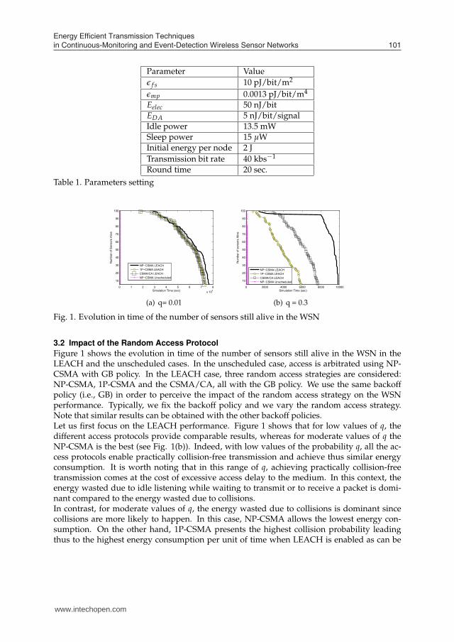
Fig. 1. Evolution in time of the number of sensors still alive in the WSN
3.2 Impact of the Random Access Protocol
Figure 1 shows the evolution in time of the number of sensors still alive in the WSN in theLEACH and the unscheduled cases. In the unscheduled case, access is arbitrated using NP-CSMA with GB policy. In the LEACH case, three random access strategies are considered:NP-CSMA, 1P-CSMA and the CSMA/CA, all with the GB policy. We use the same backoffpolicy (i.e., GB) in order to perceive the impact of the random access strategy on the WSNperformance. Typically, we fix the backoff policy and we vary the random access strategy.Note that similar results can be obtained with the other backoff policies.Let us first focus on the LEACH performance. Figure 1 shows that for low values of q, thedifferent access protocols provide comparable results, whereas for moderate values of q theNP-CSMA is the best (see Fig. 1(b)). Indeed, with low values of the probability q, all the ac-cess protocols enable practically collision-free transmission and achieve thus similar energyconsumption. It is worth noting that in this range of q, achieving practically collision-freetransmission comes at the cost of excessive access delay to the medium. In this context, theenergy wasted due to idle listening while waiting to transmit or to receive a packet is domi-nant compared to the energy wasted due to collisions.In contrast, for moderate values of q, the energy wasted due to collisions is dominant sincecollisions are more likely to happen. In this case, NP-CSMA allows the lowest energy con-sumption. On the other hand, 1P-CSMA presents the highest collision probability leadingthus to the highest energy consumption per unit of time when LEACH is enabled as can be
www.intechopen.com
Sustainable Wireless Sensor Networks102
0.1 0.2 0.3 0.4 0.5 0.6 0.7 0.8 0.9 110−4
10−3
10−2
q
Ene
rgy
Con
usm
ptio
n pe
r Uni
t of T
ime
per S
enso
r (J)
NP−CSMA LEACH1P−CSMA LEACHCSMA/CA LEACHNP−CSMA Unscheduled
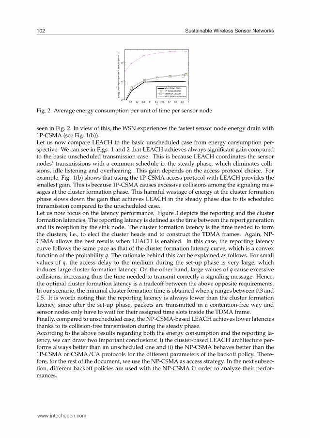
Fig. 2. Average energy consumption per unit of time per sensor node
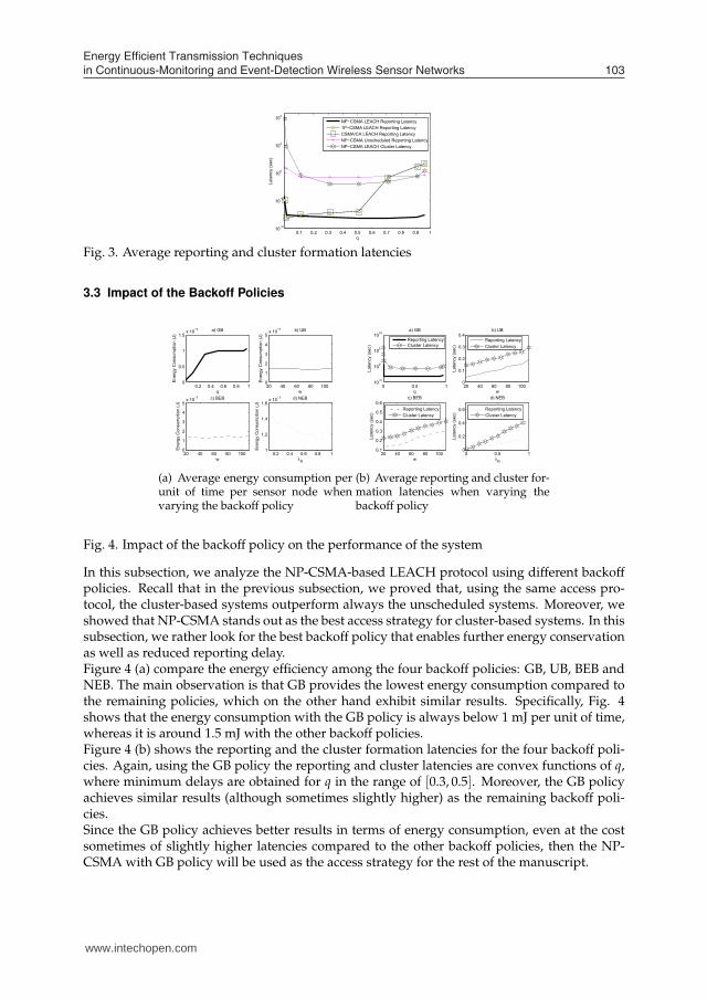
seen in Fig. 2. In view of this, the WSN experiences the fastest sensor node energy drain with1P-CSMA (see Fig. 1(b)).Let us now compare LEACH to the basic unscheduled case from energy consumption per-spective. We can see in Figs. 1 and 2 that LEACH achieves always significant gain comparedto the basic unscheduled transmission case. This is because LEACH coordinates the sensornodes’ transmissions with a common schedule in the steady phase, which eliminates colli-sions, idle listening and overhearing. This gain depends on the access protocol choice. Forexample, Fig. 1(b) shows that using the 1P-CSMA access protocol with LEACH provides thesmallest gain. This is because 1P-CSMA causes excessive collisions among the signaling mes-sages at the cluster formation phase. This harmful wastage of energy at the cluster formationphase slows down the gain that achieves LEACH in the steady phase due to its scheduledtransmission compared to the unscheduled case.Let us now focus on the latency performance. Figure 3 depicts the reporting and the clusterformation latencies. The reporting latency is defined as the time between the report generationand its reception by the sink node. The cluster formation latency is the time needed to formthe clusters, i.e., to elect the cluster heads and to construct the TDMA frames. Again, NP-CSMA allows the best results when LEACH is enabled. In this case, the reporting latencycurve follows the same pace as that of the cluster formation latency curve, which is a convexfunction of the probability q. The rationale behind this can be explained as follows. For smallvalues of q, the access delay to the medium during the set-up phase is very large, whichinduces large cluster formation latency. On the other hand, large values of q cause excessivecollisions, increasing thus the time needed to transmit correctly a signaling message. Hence,the optimal cluster formation latency is a tradeoff between the above opposite requirements.In our scenario, the minimal cluster formation time is obtained when q ranges between 0.3 and0.5. It is worth noting that the reporting latency is always lower than the cluster formationlatency, since after the set-up phase, packets are transmitted in a contention-free way andsensor nodes only have to wait for their assigned time slots inside the TDMA frame.Finally, compared to unscheduled case, the NP-CSMA-based LEACH achieves lower latenciesthanks to its collision-free transmission during the steady phase.According to the above results regarding both the energy consumption and the reporting la-tency, we can draw two important conclusions: i) the cluster-based LEACH architecture per-forms always better than an unscheduled one and ii) the NP-CSMA behaves better than the1P-CSMA or CSMA/CA protocols for the different parameters of the backoff policy. There-fore, for the rest of the document, we use the NP-CSMA as access strategy. In the next subsec-tion, different backoff policies are used with the NP-CSMA in order to analyze their perfor-mances.
0.1 0.2 0.3 0.4 0.5 0.6 0.7 0.8 0.9 110−4
10−2
100
102
104
q
Late
ncy
(sec
)
NP−CSMA LEACH Reporting Latency1P−CSMA LEACH Reporting LatencyCSMA/CA LEACH Reporting LatencyNP−CSMA Unscheduled Reporting LatencyNP−CSMA LEACH Cluster Latency
20 40 60 80 1000
1
2
3
4
5x 10⁻³
w
Ene
rgy
Con
sum
ptio
n (J
)
b) UB
20 40 60 80 1000
1
2
3
4
5x 10⁻³
w
Ene
rgy
Con
sum
ptio
n (J
)
c) BEB
0.2 0.4 0.6 0.8 11
1.2
1.4
1.6x 10⁻³
R
Ene
rgy
Con
sum
ptio
n (J
)
d) NEB
0.2 0.4 0.6 0.8 10
0.5
1
1.5x 10⁻³
q
Ene
rgy
Con
sum
ptio
n (J
)
a) GB
0 0.5 110−5
100
105
1010
q
Late
ncy
(sec
)
a) GB
20 40 60 80 1000
0.1
0.2
0.3
0.4
w
Late
ncy
(sec
)
b) UB
20 40 60 80 1000.1
0.2
0.3
0.4
0.5
0.6
w
Late
ncy
(sec
)
c) BEB
0 0.5 10
0.2
0.4
0.6
R
Late
ncy
(sec
)
d) NEB
Reporting LatencyCluster Latency
Reporting LatencyCluster Latency
Reporting LatencyCluster Latency
Reporting LatencyCluster Latency
www.intechopen.com
Energy Eficient Transmission Techniques in Continuous-Monitoring and Event-Detection Wireless Sensor Networks 103
0.1 0.2 0.3 0.4 0.5 0.6 0.7 0.8 0.9 110−4
10−3
10−2
q
Ene
rgy
Con
usm
ptio
n pe
r Uni
t of T
ime
per S
enso
r (J)
NP−CSMA LEACH1P−CSMA LEACHCSMA/CA LEACHNP−CSMA Unscheduled
0.1 0.2 0.3 0.4 0.5 0.6 0.7 0.8 0.9 110−4
10−2
100
102
104
q
Late
ncy
(sec
)
NP−CSMA LEACH Reporting Latency1P−CSMA LEACH Reporting LatencyCSMA/CA LEACH Reporting LatencyNP−CSMA Unscheduled Reporting LatencyNP−CSMA LEACH Cluster Latency
Fig. 3. Average reporting and cluster formation latencies
3.3 Impact of the Backoff Policies
20 40 60 80 1000
1
2
3
4
5x 10⁻³
w
Ene
rgy
Con
sum
ptio
n (J
)
b) UB
20 40 60 80 1000
1
2
3
4
5x 10⁻³
w
Ene
rgy
Con
sum
ptio
n (J
)
c) BEB
0.2 0.4 0.6 0.8 11
1.2
1.4
1.6x 10⁻³
λR
Ene
rgy
Con
sum
ptio
n (J
)
d) NEB
0.2 0.4 0.6 0.8 10
0.5
1
1.5x 10⁻³
q
Ene
rgy
Con
sum
ptio
n (J
)
a) GB
(a) Average energy consumption perunit of time per sensor node whenvarying the backoff policy
0 0.5 110−5
100
105
1010
q
Late
ncy
(sec
)
a) GB
20 40 60 80 1000
0.1
0.2
0.3
0.4
w
Late
ncy
(sec
)
b) UB
20 40 60 80 1000.1
0.2
0.3
0.4
0.5
0.6
w
Late
ncy
(sec
)
c) BEB
0 0.5 10
0.2
0.4
0.6
λR
Late
ncy
(sec
)
d) NEB
Reporting LatencyCluster Latency
Reporting LatencyCluster Latency
Reporting LatencyCluster Latency
Reporting LatencyCluster Latency
(b) Average reporting and cluster for-mation latencies when varying thebackoff policy
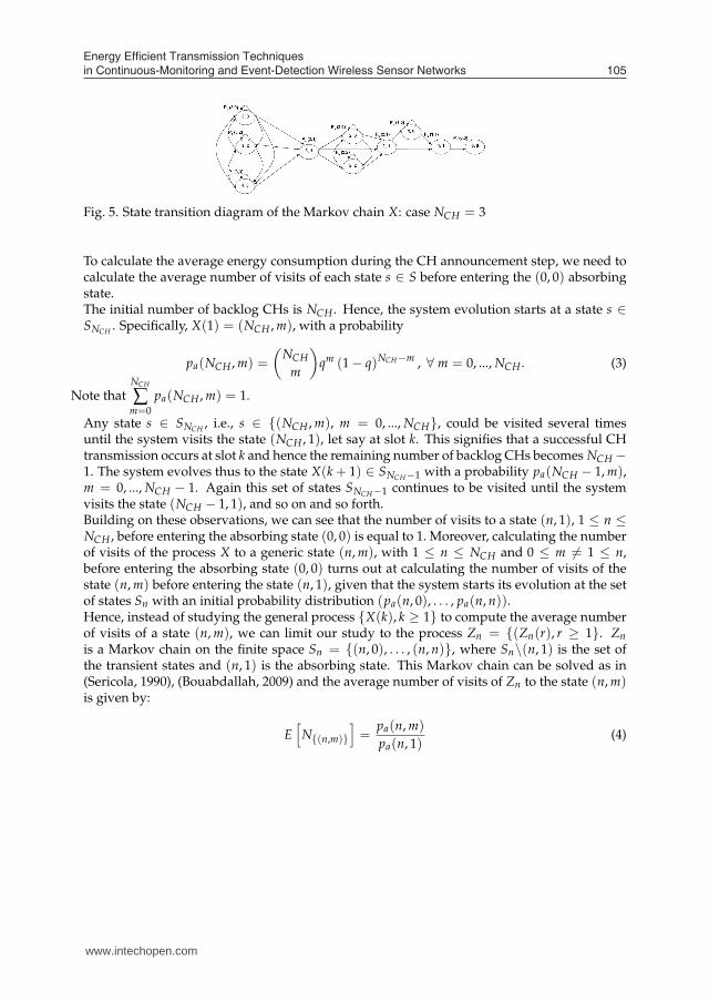
Fig. 4. Impact of the backoff policy on the performance of the system
In this subsection, we analyze the NP-CSMA-based LEACH protocol using different backoffpolicies. Recall that in the previous subsection, we proved that, using the same access pro-tocol, the cluster-based systems outperform always the unscheduled systems. Moreover, weshowed that NP-CSMA stands out as the best access strategy for cluster-based systems. In thissubsection, we rather look for the best backoff policy that enables further energy conservationas well as reduced reporting delay.Figure 4 (a) compare the energy efficiency among the four backoff policies: GB, UB, BEB andNEB. The main observation is that GB provides the lowest energy consumption compared tothe remaining policies, which on the other hand exhibit similar results. Specifically, Fig. 4shows that the energy consumption with the GB policy is always below 1 mJ per unit of time,whereas it is around 1.5 mJ with the other backoff policies.Figure 4 (b) shows the reporting and the cluster formation latencies for the four backoff poli-cies. Again, using the GB policy the reporting and cluster latencies are convex functions of q,where minimum delays are obtained for q in the range of [0.3, 0.5]. Moreover, the GB policyachieves similar results (although sometimes slightly higher) as the remaining backoff poli-cies.Since the GB policy achieves better results in terms of energy consumption, even at the costsometimes of slightly higher latencies compared to the other backoff policies, then the NP-CSMA with GB policy will be used as the access strategy for the rest of the manuscript.
www.intechopen.com

Sustainable Wireless Sensor Networks104
4. Mathematical Model for LEACH
In this section, we present a mathematical model for the LEACH-enabled WSNs. Comparedto (Heinzelman et al., 2002), we consider the energy consumption and the delay introduced bythe cluster formation phase. We present explicit expressions for the average energy consumedper unit of time by a sensor node, the average reporting latency and the average cluster for-mation time. We consider the LEACH protocol with the NP-CSMA access strategy and theGB policy, where a packet transmission is done with probability q. It is important to note thatthe results provided by this model will be used as baselines to which the CM-EDR improve-ments are compared. In the next section, we present the analytical model when the CM-EDRstrategy is enabled.
4.1 Energy Consumption Analysis
At the beginning of each new cycle or round, a new set of NCH CHs is elected. The CH role isrotated among all sensor nodes in order to balance the energy consumption inside the WSN.The cluster formation phase can be divided into three steps: CH announcement, CM join andCH schedules. In the first step, each elected CH advertises all the sensor nodes in the WSN.Once the CH announcement step is completed, each sensor node transmits a CM join messageto its associated CH. Based on this information, each CH transmits a message indicating theschedule to its associated CMs. In what follows, each step will be analyzed separately.
4.1.1 CH announcement step
At the beginning of the set-up phase, all the elected CHs try to advertise the remaining sensornodes at the same time, leading thus to a collision occurrence. All the CH nodes undergohence the backoff procedure. Accordingly, the channel is divided into time slots that can beused by the CHs to transmit their announcement messages. The duration of a time slot tsig isby definition the time that takes a sensor to transmit a control packet.In order to calculate the energy consumption in the CH announcement step, we consider thatat any time slot, the system can be defined according to the number of potential nodes thatcan initiate transmission, n, and the number of actual transmissions made, m, at the begin-ning of the time slot. Hence, the system can be described by the duple (n, m). We makeuse of a transitory Markov chain in order to derive the average number of time slots that theLEACH system remains in the state (n, m) at the cluster formation phase, where n representsthe number of CHs with a backlog packet (i.e., CHs that have not yet transmitted correctlytheir announcement messages) at the beginning of the slot k and m ∈ {0, ..., n} represents thenumber of nodes that transmit on the slot k.Let X(k) be the system state at the slot k defined by the tuple (n, m). Then, the event {X(k) =(n, 0)} means that no node transmits on the slot k and hence the slot remains free. {X(k) =(n, m)} with m > 1 means that a collision occurs on the slot k. Finally, {X(k) = (n, 1)} meansthat a successful transmission of a CH announcement message is achieved on the slot k. Inthis case, the next slot system state will be X(k + 1) = (n − 1, m′) with m′ ∈ {0, ..., n − 1}.The transmission of each backlog node on a slot is achieved according to a geometric processwith a probability q. Hence, the process {X(k), k ≥ 1} is a discrete time Markov chain withthe state space S = {(n, m) | 0 ≤ n ≤ NCH , 0 ≤ m ≤ n} as depicted in Fig. 5. The space stateS can be also expressed as follows:
S =NCH⋃
n=0
Sn, with Sn = {(n, m) | 0 ≤ m ≤ n} (2)
www.intechopen.com
Energy Eficient Transmission Techniques in Continuous-Monitoring and Event-Detection Wireless Sensor Networks 105
Fig. 5. State transition diagram of the Markov chain X: case NCH = 3
To calculate the average energy consumption during the CH announcement step, we need tocalculate the average number of visits of each state s ∈ S before entering the (0, 0) absorbingstate.The initial number of backlog CHs is NCH . Hence, the system evolution starts at a state s ∈SNCH
. Specifically, X(1) = (NCH , m), with a probability
pa(NCH , m) =
(
NCH
m
)
qm (1 − q)NCH−m , ∀ m = 0, ..., NCH . (3)
Note thatNCH
∑m=0
pa(NCH , m) = 1.
Any state s ∈ SNCH, i.e., s ∈ {(NCH , m), m = 0, ..., NCH}, could be visited several times
until the system visits the state (NCH , 1), let say at slot k. This signifies that a successful CHtransmission occurs at slot k and hence the remaining number of backlog CHs becomes NCH −1. The system evolves thus to the state X(k + 1) ∈ SNCH−1 with a probability pa(NCH − 1, m),m = 0, ..., NCH − 1. Again this set of states SNCH−1 continues to be visited until the systemvisits the state (NCH − 1, 1), and so on and so forth.Building on these observations, we can see that the number of visits to a state (n, 1), 1 ≤ n ≤NCH , before entering the absorbing state (0, 0) is equal to 1. Moreover, calculating the numberof visits of the process X to a generic state (n, m), with 1 ≤ n ≤ NCH and 0 ≤ m �= 1 ≤ n,before entering the absorbing state (0, 0) turns out at calculating the number of visits of thestate (n, m) before entering the state (n, 1), given that the system starts its evolution at the setof states Sn with an initial probability distribution (pa(n, 0), . . . , pa(n, n)).Hence, instead of studying the general process {X(k), k ≥ 1} to compute the average numberof visits of a state (n, m), we can limit our study to the process Zn = {(Zn(r), r ≥ 1}. Zn
is a Markov chain on the finite space Sn = {(n, 0), . . . , (n, n)}, where Sn\(n, 1) is the set ofthe transient states and (n, 1) is the absorbing state. This Markov chain can be solved as in(Sericola, 1990), (Bouabdallah, 2009) and the average number of visits of Zn to the state (n, m)is given by:
E[
N{(n,m)}
]
=pa(n, m)
pa(n, 1)(4)
www.intechopen.com
Sustainable Wireless Sensor Networks106
Accordingly, the total energy consumption in the WSN during the CH announcement stepcan be calculated as follows:
ECH_Announ = f (NCH , lsig) = NCH Etx(lsig, dmax) + (N − NCH) Erx(lsig)
+NCH
∑n=1
n
∑m=1
E[
N{(n,m)}
]
(
mEtx(lsig, dmax) + (N − m) Erx(lsig)
)
+ NEidletsig
NCH
∑n=1
E[
N{(n,0)}
]
(5)
where lsig denotes the size of a control packet, dmax =√
2M the diameter of the M × Msquare supervised area and Eidle the average amount of energy consumed per unit of time bya sensor node in the idle state. We highlight that the first element of (5) corresponds to theenergy dissipated in the WSN due to the first collision among all the CHs when attemptingto send for the first time all together their announcement messages at the beginning of theset-up phase. The remaining elements of (5) correspond to the energy consumption duringthe backoff procedure that undergo the NCH CHs.
4.1.2 CM join step
As explained before, once the CH announcement step is completed, each sensor node trans-mits a CM join message to its associated CH. Similarly to the CH announcement step, theN − NCH sensor nodes try to join their CHs at the same time, leading thus to a collision occur-rence. Then, the sensor nodes enter in backoff procedure to transmit their CM join messages.Following the same reasoning as in the CH announcement step (i.e., using (5)), we obtain theaverage energy dissipated during the CM join step as ECM_Join = f (N − NCH , lsig).
4.1.3 CH schedules step
In this step, each CH transmits a message indicating the schedule to its associated CMs. Usingthe same reasoning as before, the average energy consumed during the CH schedules step isgiven by ECH_Sched = f (NCH , lsig).Finally, the average amount of energy dissipated to form clusters is:
ESet−up(LEACH)=ECH_Announ+ECM_Join+ECH_Sched (6)
4.1.4 Energy consumption in the steady phase
Let us now calculate the average amount of energy consumed during the steady phase, whereeach CH receives periodically a TDMA frame from its CMs. In our study, we assume that theN sensor nodes are uniformly distributed in the supervised area. Hence, there are on averageN/NCH nodes, including the CH, in each cluster.In continuous-monitoring WSNs, each sensor node senses its area periodically, each Tsensing
period of time, where Tsensing ≥ Tf rame. We note that Tf rame = NNCH
tdata is the duration of aTDMA frame, where tdata is the duration of a time slot needed by a sensor to transmit a datapacket of size ldata. In the particular case where Tsensing = Tf rame, the WSN operates in thesaturation regime, i.e., a sensor node always has data to send to the sink node. Since eachsensor node wakes up only during its attributed time slot, then the energy consumed by a CMi node during a sensing period Tsensing is:
ECM(i) =(
Tsensing − tdata
)
Esleep + Etx(ldata, dCM(i)_CH) (7)
www.intechopen.com
Energy Eficient Transmission Techniques in Continuous-Monitoring and Event-Detection Wireless Sensor Networks 107
where Esleep is the average amount of energy consumed by a sensor node per unit of timein the sleep state and dCM(i)_CH is the distance between the CM node i and its associatedCH. In (Heinzelman et al., 2002), it was demonstrated that if the density of nodes is uniformthroughout the cluster area, then the expected square distance from the CM nodes to the CH
is given by E[
(dCM_CH)2]
= M2
2πNCHwhere M is the side length of the square supervised area.
Hence the average amount of energy consumed by a CM node during a sensing period is:
ECM(LEACH) =(
Tsensing − tdata
)
Esleep + Etx
(
ldata,M√
2πNCH
)
In turn, each CH consumes energy in receiving and aggregating the data sent by its CMs aswell as in the transmission of that aggregated data to the sink node. The energy consumed bya CH node during a TDMA frame is therefore:
ECH_ f rame(LEACH) =
(
N
NCH− 1
)
Erx(ldata) +N
NCHldataEDA + Etx(ldata, dCH_SN)
where dCH_SN is the average distance from the CH to the sink node. Thus, the energy con-sumed by a CH node during a sensing period is:
ECH(LEACH) = ECH_ f rame(LEACH) +(
Tsensing − Tf rame
)
Esleep
The energy consumed in the network during a sensing period is therefore:
EWSN(LEACH) = NCH
((
N
NCH− 1
)
ECM(LEACH) + ECH(LEACH)
)
and the total energy consumed in the network during the steady phase is:
ESteady(LEACH) = EWSN(LEACH)×Tround − Tset−up(LEACH)
Tsensing
where Tround is the round time after which the CH nodes are elected anew andTset−up(LEACH) is the average time spent in the cluster formation phase, which will be de-rived in the next subsection.Finally, we obtain the average amount of energy consumed by each sensor node in the WSNper unit of time when the basic LEACH clustering is adopted:
Esensor(LEACH) =ESteady(LEACH) + ESet−up(LEACH)
NTround(8)
4.2 Latency Analysis
In this subsection we derive both the average cluster formation time and the average reportinglatency.
www.intechopen.com
Sustainable Wireless Sensor Networks108
4.2.1 The average cluster formation time
It is the time needed to form the clusters, i.e., to perform the CH announcement, the CM joinand the CH schedules steps. Using the same model introduced in the previous section, theCH announcement time is simply the time elapsed from the beginning of the cluster formationprocedure to the instant where all the CHs successfully transmit their announcement message.As such, the CH announcement time can be expressed as follows:
TCH_Announ = g(NCH , tsig) =
(
1 +NCH
∑n=1
n
∑m=0
E[
N{(n,m)}
]
)
tsig (9)
We highlight that (9) is the sum of the time lost due to the first collision among all the CHswhen attempting to send for the first time all together their announcement messages (i.e., tsig)and the average duration of the backoff procedure that undergo the NCH CHs.Following the same reasoning, we obtain the average time spent in the CM join and the CHschedules steps as follows:
TCM_Join = g(N − NCH , tsig) (10)
TCH_Sched = g(NCH , tsig) (11)
Finally, the average time needed to form clusters is:
TSet−up(LEACH) = TCH_Announ + TCM_Join + TCH_Sched (12)
4.2.2 The average reporting latency
It is the time needed by a generated report to be received by the sink node. In continuous-monitoring WSNs, the sensor nodes produce data information at the beginning of each sens-ing period. In the steady phase, the average reporting time is simply the transmission timeof a TDMA frame. Considering the extra delay spent in the construction of the clusters, thereporting latency increases slightly as follows:
Treporting(LEACH) = Tf rame +Tset−up(LEACH)Tsensing
Tround(13)
5. Energy Efficient Protocols for Continuous-Monitoring Applications
This section introduces our CM-EDR scheme. In the previous section, we presented a math-ematical analysis for the classical continuous-monitoring LEACH WSNs. In this section, weanalyze the corresponding CM-EDR-aware extension. Comparing the new results, i.e., the av-erage energy consumption, the average reporting latency and the average cluster formationtime, to that obtained with the classical approach, we can gauge the benefits introduced bythe proposed CM-EDR technique.
5.1 The CM-EDR Scheme
The main idea behind the CM-EDR introduction is avoiding the extra transmission of nonrelevant data information, typical in classical continuous-monitoring WSNs. With CM-EDR,continuous-monitoring does not imply indeed continuous reporting. By reporting onlyrelevant data, the sink node would gather exactly the same information as with classicalcontinuous-monitoring applications while receiving less reports and thus dissipating less en-ergy.
www.intechopen.com
Energy Eficient Transmission Techniques in Continuous-Monitoring and Event-Detection Wireless Sensor Networks 109
Enabling the CM-EDR technique, each sensor node continues to produce periodically datainformation. However, the sensed information is reported to the sink node only if it differsfrom the last transmitted data information. In doing so, the sensor node dissipates also lessenergy in communications, achieving thus significant energy conservation. Clearly, the energyconsumption will greatly depend on the rate of variation of the phenomenon that the sensorsare monitoring.With CM-EDR, each sensor node needs to storage the last transmitted data (i.e., only a singlepacket). Evidently, this does not entail the need to increase the memory capacity of sensornodes. Following to each periodic observation, the sensor node compares the new readingto the stored one. If both readings are similar, the new generated data packet is discarded.Otherwise, the new information is reported to the sink node and the stored information isupdated. In this case, we deal with relevant data, referred to us also as an event.It is worth noting that our approach can be seen as a new alternative to reduce the trans-mission of redundant information, by profiting from the natural temporal correlation amongthe sensed data information. Our technique complement the data fusion or aggregation tech-niques (Intanagonwiwat et al., 2000) – (Larrea er al., 2007) and the spatial-correlation basedschemes (Bouabdallah et al., 2009) – (Vuran et al., 2006).
5.2 Analytical Model for the CM-EDR-enabled LEACH WSNs
This subsection extends the analysis done in section IV to the case where the CM-EDR tech-nique is enabled. Since the CM-EDR technique does not affect the set-up phase, the analysisfor this phase remains unchanged. Hereafter, we focus on the analysis of the steady phase.Assume that the variations on the sensed information, for example the temperature around asensor node, happen following a Poisson process of rate λ. In other words, the time betweentwo variations of the temperature is exponentially distributed. In our case, each sensor nodesenses its area periodically, each Tsensing period of time. Tsensing is chosen by the administratorsuch that the probability that two or more changes on the sensed information occurs duringTsensing be negligible, i.e., be below a certain threshold ε as follows:
Pr{Nevent ≥ 2} = 1 − e−λTsensing − λTsensinge−λTsensing ≤ ε (14)
where Nevent is the number of changes that occurs on the sensed information during Tsensing.As such, Tsensing must verify:
Tsensing ≤ sup{t | 1 − e−λt − λte−λt ≤ ε} (15)
Hence, the probability that the sensed information be relevant, for example the temperaturechanges between two observations, i.e., during the last Tsensing period, is given by:
Pevent ≃ Pr{Nevent = 1} = λTsensinge−λTsensing (16)
Based on this model, during the steady phase each CM-EDR-enabled sensor node transmitson its reserved slot (i.e., uses the current frame) according to a geometric process of probabilityPevent. Assuming that a CM node enters the sleep mode during the sensing period and wakesup only on its associated slot if it has relevant data to transmit, the average amount of energyconsumed by a CM node during a sensing period is:
ECM(CM−EDR) = PeventECM(LEACH) + (1 − Pevent) TsensingEsleep
www.intechopen.com
Sustainable Wireless Sensor Networks110
On the other hand, each CH consumes energy in receiving and aggregating the data sent byits CMs as well as in the transmission of that aggregated data to the sink node. The averageamount of energy dissipated by a CH node in the reception of a frame can be given by:
ECH_rec =
⌈
NNCH
⌉
−1
∑k=0
(
⌈
NNCH
⌉
−1
k
)
(Pevent)k(1−Pevent)
⌈
NNCH
⌉
−1−k
×
(
kErx(ldata) + tdataEidle
(⌈
N
NCH
⌉
−1−k
))
Assuming perfect data aggregation, the average amount of energy dissipated by a CH nodedue to aggregation is:
ECH_agg =
⌈
NNCH
⌉
∑k=0
(
⌈
NNCH
⌉
k
)
(Pevent)k (1 − Pevent)
⌈
NNCH
⌉
−k× (kldataEDA)
The average amount of energy dissipated by a CH for a possible transmission of the aggre-gated data to the sink node is:
ECH_tr =
(
1 − (1 − Pevent)N
NCH
)
Etx(ldata, dCH_SN)
Hence, the total energy consumed by a CH node during a TDMA frame when CM-EDR isenabled is:
ECH_ f rame(CM−EDR) = ECH_rec+ECH_agg+ECH_tr (17)
and the energy consumed by a CH node during a sensing period is:
ECH(CM−EDR) = ECH_ f rame(CM−EDR) +(
Tsensing − Tf rame
)
Esleep
The energy consumed in the network during a sensing period is therefore:
EWSN(CM−EDR) = NCH
(
ECH(CM−EDR) +
(
N
NCH−1
)
ECM(CM−EDR)
)
and the total energy consumed in the network during the steady phase is:
ESteady(CM−EDR) = EWSN(CM−EDR)×Tround − Tset−up(LEACH)
Tsensing
Finally, we obtain the average amount of energy consumed by each sensor node in the WSNper unit of time when the CM-EDR option is enabled:
Esensor(CM−EDR) =
(
ESteady(CM−EDR) + ESet−up(LEACH)
)
1
NTround
With regard to the latency performance, it is worth noting that the CM-EDR scheme does notimpact the latency compared to the classical LEACH case. Indeed, a relevant data packet isreceived by the sink node at the same time whether the CM-EDR mechanism is enabled ornot. The CM-EDR mechanism avoids only the transmission of non relevant data.
www.intechopen.com

Energy Eficient Transmission Techniques in Continuous-Monitoring and Event-Detection Wireless Sensor Networks 111
5.3 Optional Mechanism for CM-EDR-enabled Cluster-Based WSNs
Using CM-EDR, a CH node transmits to the sink node only if it senses or receives relevantdata from its CMs. As such, the CH may not transmit to the sink during a long period ifit does not receive any relevant information. Even though, it dissipates energy due to idlelistening. The energy wasted due to idle listening is far from being negligible and can accountfor a significant portion of the energy a sensor dissipates in some cases (Woo et al., 2001).To achieve further energy conservation, the CH will be allowed with the optional CM-EDR(OCM-EDR) to enter sleep mode during Nsleep sensing periods if it does not receive any rel-evant data during Nidle consecutive frames. The CH assumes indeed that the supervised en-vironment is "calm" and it is improbable that an event occurs in the next sensing periods. Inthis case, the CH advertises its CMs that it will undergo the sleep state during Nsleep sensingperiods. However, during this period, a CM node may sense a relevant data that needs tobe reported immediately (i.e., in the current frame) to the sink node, otherwise continuous-monitoring property is lost. To do so, the sensor node is allowed to transmit directly thisinformation to the sink node during its reserved slot.Let us now calculate the average energy consumption by a sensor node when this optionalmechanism is enabled. Let Y(k) be the CH state at the sensing period k of the steady phasedefined by the tuple (i, j), where i = 0 if the CH is in the sleep state and i = 1 otherwise.Moreover, if i = 0, j = 1, ..., Nsleep signifies that the CH has been for j sensing periods inthe sleep state (including the current sensing period); otherwise (i.e., if i = 1) j = 1, ..., Nidle
indicates the number of consecutive empty (non relevant) frames that has received the CH.The process Y = {Y(k), k ≥ 1} is a discrete time Markov chain with the state space S = {(i, j)| 0 ≤ i ≤ 1, 1 ≤ j ≤ Nsleep1{
i=0} + Nidle1{
i=1}}. For every s ∈ S, we denote by
Πs = limk→+∞
Pr{Y(k) = s}
where Π = [Πs] is the steady state distribution of the Markov chain Y, which satisfies
ΠP = Π and ∑s∈S
Πs = 1, (18)
and P = (P(s, s′)), s = (i, j) , s′ = (i′, j′) ∈ S, is the transition probability matrix of Y given by:
P(s, s′) =
Pf ree if(
i = i′ = 1 and j′ = j + 1)
;
1 − Pf reeif(
s′ = (1, 1) and s = (1, j)with j < Nidle
)
;
1 if
(
i = i′ = 0 and j′ = j + 1)
or(
s = (1, Nidle) ands′ = (0, 1)
)
or(
s = (0, Nsleep) and
s′ = (1, 1))
;0 otherwise.
(19)
where Pf ree is the probability that the CH node does not transmit to the sink node since it hasnot any relevant data to forward. Pf ree is given by:
Pf ree = (1 − Pevent)N
NCH (20)
www.intechopen.com
Sustainable Wireless Sensor Networks112
Let K =
⌈
Tround
Tsensing
⌉
denote the number of sensing periods during a round. We denote by
PCH_sleep the percentage of sensing periods in a round, during which a CH is in the sleepstate. PCH_sleep can be expressed as follows:
PCH_sleep =1
K
Nsleep
∑j=1
V(0,j)(K) (21)
where V(0,j)(K) is the number of visits to the state (0, j) during a round, i.e., during the K firsttransitions of process Y. Then, PCH_sleep is given by:
PCH_sleep =1
K
Nsleep
∑j=1
K
∑k=1
Pr{Y(k) = (0, j)}
=1
K
Nsleep
∑j=1
K
∑k=1
(
αPk)
(0,j)(22)
where α is the initial probability distribution of Y and(
αPk)
(0,j)is the (0, j) element of the
vector αPk. Note that when K goes to the infinity, PCH_sleep denotes the probability that a CHis in the sleep state during a sensing period, i.e.,
limK→+∞
PCH_sleep = ∑s∈S
Πs1{i=0
} =Nsleep
∑j=1
Π(0,j) (23)
Deriving the steady state distribution of the Markov chain Y, we get
limK→+∞
PCH_sleep =Nsleep
∑j=1
Nsleep
(
Pf ree
)Nidle−1Π(1,1)
=Nsleep
(
1 − Pf ree
) (
Pf ree
)Nidle−1
1 −(
Pf ree
)Nidle
+Nsleep
(
1 − Pf ree
)(
Pf ree
)Nidle−1(24)
Now, we can derive the average amount of energy consumed by a CM node during a sensingperiod as follows:
ECM(OCM−EDR) = (1 − Pevent) TsensingEsleep
+Pevent
(
1−PCH_sleep
)
ECM(LEACH)
+PeventPCH_sleep
(
Etx (ldata, dCM_SN)
+(
Tsensing − tdata
)
Esleep
)
(25)
0 2 4 6 8 100
1
2
x 10−4
Ave
rage
Ene
rgy
Con
sum
ptio
n (J
)
CM−EDR (Simul)OCM−EDR (Simul)CM−EDR (Anal)OCM−EDR (Anal)
0 2 4 6 8 1010−5
10−4
10−3
10−2
10−1
Ave
rage
Ene
rgy
Con
sum
ptio
n (J
)
Basic LEACHUnscheduledCM−EDROCM−EDR
www.intechopen.com
Energy Eficient Transmission Techniques in Continuous-Monitoring and Event-Detection Wireless Sensor Networks 113
0 2 4 6 8 100
1
2
x 10−4
λ
Ave
rage
Ene
rgy
Con
sum
ptio
n (J
)
CM−EDR (Simul)OCM−EDR (Simul)CM−EDR (Anal)OCM−EDR (Anal)
(a) Proposed protocols
0 2 4 6 8 1010−5
10−4
10−3
10−2
10−1
λ
Ave
rage
Ene
rgy
Con
sum
ptio
n (J
)
Basic LEACHUnscheduledCM−EDROCM−EDR
(b) Comparison with LEACH
Fig. 6. Average energy consumption per unit of time per sensor node
where dCM_SN is the average distance between a CM node and the sink node. On the otherhand, the average energy consumed by a CH node during a sensing period with OCM-EDRis:
ECH(OCM−EDR) =(
1 − PCH_sleep
)
ECH(CM−EDR) + PCH_sleepTsensingEsleep
Using the expressions of ECM(OCM−EDR) and ECH(OCM−EDR) given by (we derive in theway as in (18) the average energy consumed by a sensor node with OCM-EDR.
5.4 Numerical Results
We now evaluate the efficiency of our proposed mechanisms We first study the gain that theyintroduced using four baseline examples: the case of unscheduled WSNs and three variants ofcluster-based WSNs. Then, we compare between the CM-EDR and OCM-EDR mechanisms.A simulation model has been developed in order to validate the analytic results. The systemof WSNs was implemented as a discrete event simulation. Numerous evaluations were per-formed in order to confirm the analytic results. In all cases, the results matched very closely.Figure 6 (a) compares the simulation results of the energy consumption with CM-EDR to thatgiven by equation (18) as a function of the rate λ. In this case, Tsensing is chosen such that it
verifies the constraint given by (15) with ε = 10−4. For the OCM-EDR mechanism, Figure 6compares the simulation results of the energy consumption as a function of λ. In this case,we consider Nidle = 1, Nsleep = 10 and ε = 10−4. Figure 6 (a) shows that there is a good fitbetween the simulation and analytical results, which exhibits the accuracy of our analysis.For the remainder of the results, it has been confirmed that there is a good fit between thesimulation and analytical results. Therefore, for presentation purposes, all remaining figuresshow only the simulation results. We assume the same network topology used in the previoussections, i.e., 100 sensor node-network. We assume also that ε = 10−4, i.e., Tsensing = sup{t |
1− e−λt −λte−λt ≤ 10−4}. Moreover, unless explicitly notified, we consider q = 0.3, Nidle = 1and Nsleep = 10. The parameters setting in our experiments are listed in table I.According to the results presented in Fig. 6 we can draw three main observations:
• Clustering achieves always significant gain in terms of energy Further energy conser-vation can be achieved when the CM-EDR mechanisms are enabled, which brings us tothe second observation.
www.intechopen.com
Sustainable Wireless Sensor Networks114
• The sensor node lifetime is increased considerably when enabling our CM-EDR mech-anisms. Clearly, the CM-EDR abilities provide an advantage over the classical WSNs,by preventing the transmission of redundant data. For reference, Fig. 6 (b) shows therelative decrease in the energy consumption by a sensor node per unit of time of theCM-EDR networks compared to the classic networks. The magnitude of the increaseregarding the sensor node lifetime decreases as the rate λ grows. In other words, therelative improvement decreases when the supervised area becomes agitated since lessnon relevant data are transmitted by the classical WSNs.
• The OCM-EDR mechanism outperforms the CM-EDR one, when we deal with calmWSNs, whereas in agitated WSNs, it is better to use the basic CM-EDR mechanism.The rationale behind this can be explained as follows. Allowing the CHs to go to sleepwith OCM-EDR results in the occurrence of expensive direct transmissions from theCMs to the sink node. In agitated environment, the energy conservation achieved atthe CHs due to their asleep abilities is dominated by the additional energy consumedat the CM nodes due to frequent direct communications to the sink node. These directcommunications become rare in calm WSNs.
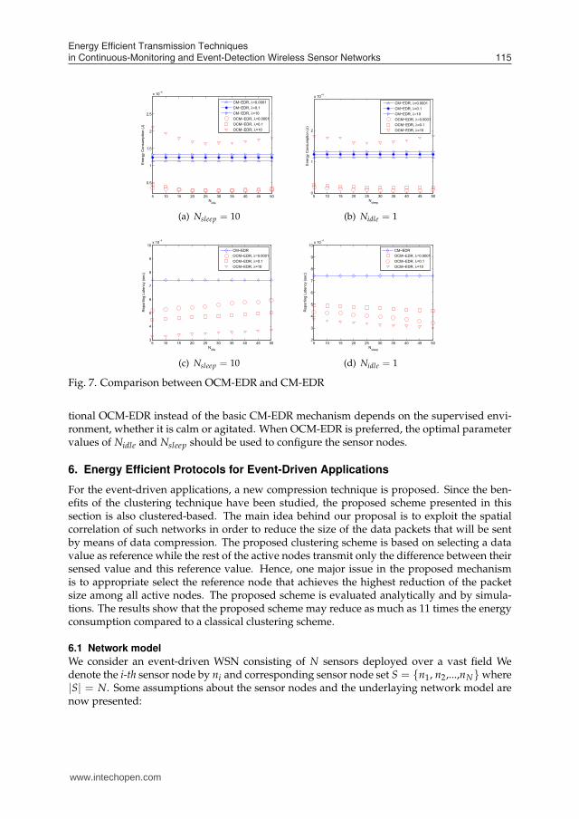
Clearly, the CM-EDR systems are a major improvement over the classic networks. Figure6(b) shows the average amount of energy consumed by a sensor node per unit of time as afunction of the rate λ. Again, we can observe that the CM-EDR abilities provide significantenergy conservation, notably in calm WSNs. This improvement decreases with λ. Moreover,enabling the optional version OCM-EDR is helpful only for small to moderate values of λ;otherwise, the basic version of CM-EDR performs better.Figure 7 provides more insight into the effectiveness of using the OCM-EDR extension in-stead of the basic CM-EDR mechanism in the context of cluster-based WSNs. In this case, thetwo variants of the CM-EDR technique are introduced over a classical LEACH WSN. Notethat similar results can be obtained when using the remaining clustering protocols. Figure 7shows the performance of OCM-EDR as a function of the setting parameters Nidle and Nsleep
for various values of the rate λ. Recall that with the optional OCM-EDR, the CH enters thesleep mode during Nsleep sensing periods if it does not receive any relevant data during Nidle
consecutive frames.The energy consumption with OCM-EDR is a convex function of Nidle (see Fig. 7(a)). Forlow values of Nidle, the CHs enter frequently to the sleep mode. Hence, the sensor nodesare most likely transmitting directly to the sink node instead of passing through the CHs.On the other hand, when Nidle gets large values, the CHs almost never enter the sleep modeand can not profit from the calm periods of the supervised environment. Hence, the energyconsumption increases. For moderate values of Nidle, the CHs enter the sleep mode withoutreally penalizing the sensor nodes. In our scenario, setting Nidle = 25 enables the minimalenergy consumption in the network (see Fig. 7(a)).In the same way, the energy consumption with OCM-EDR is a convex function of Nsleep (seeFig. 7(b)). Decreasing Nsleep, the CHs enter into the sleep state for very short periods of timeand hence can not really profit from the calm periods of the supervised environment. In ourexample, the energy consumption is minimal when Nsleep = 36 (see Fig. 7(b)).With regard to reporting latency, we can see that OCM-EDR achieves always better resultsthan the basic CM-EDR. This is because the OCM-EDR mechanism replaces some relativelylong multi-hop transmissions (i.e.,To conclude this study, we can state that the CM-EDR philosophy enables significant energyconservation while ensuring continuous-monitoring applications. The decision to use the op-
5 10 15 20 25 30 35 40 45 50
0.5
1
1.5
2
2.5
x 10−4
Nidle
Ene
rgy
Con
sum
ptio
n (J
)
CM−EDR, =0.0001CM−EDR, =0.1CM−EDR, =10OCM−EDR, =0.0001OCM−EDR, =0.1OCM−EDR, =10
5 10 15 20 25 30 35 40 45 500
1
2
x 10−4
Nsleep
Ene
rgy
Con
sum
ptio
n (J
)
CM−EDR, =0.0001CM−EDR, =0.1CM−EDR, =10OCM−EDR, =0.0001OCM−EDR, =0.1OCM−EDR, =10
5 10 15 20 25 30 35 40 45 503
4
5
6
7
8
9
10x 10−4
Nidle
Rep
ortin
g La
tenc
y (s
ec)
CM−EDROCM−EDR, =0.0001OCM−EDR, =0.1OCM−EDR, =10
5 10 15 20 25 30 35 40 45 502
3
4
5
6
7
8
9
10x 10−4
Nsleep
Rep
ortin
g La
tenc
y (s
ec)
CM−EDROCM−EDR, =0.0001OCM−EDR, =0.1OCM−EDR, =10
www.intechopen.com
Energy Eficient Transmission Techniques in Continuous-Monitoring and Event-Detection Wireless Sensor Networks 115
5 10 15 20 25 30 35 40 45 50
0.5
1
1.5
2
2.5
x 10−4
Nidle
Ene
rgy
Con
sum
ptio
n (J
)
CM−EDR, λ=0.0001CM−EDR, λ=0.1CM−EDR, λ=10OCM−EDR, λ=0.0001OCM−EDR, λ=0.1OCM−EDR, λ=10
(a) Nsleep = 10
5 10 15 20 25 30 35 40 45 500
1
2
x 10−4
Nsleep
Ene
rgy
Con
sum
ptio
n (J
)
CM−EDR, λ=0.0001CM−EDR, λ=0.1CM−EDR, λ=10OCM−EDR, λ=0.0001OCM−EDR, λ=0.1OCM−EDR, λ=10
(b) Nidle = 1
5 10 15 20 25 30 35 40 45 503
4
5
6
7
8
9
10x 10−4
Nidle
Rep
ortin
g La
tenc
y (s
ec)
CM−EDROCM−EDR, λ=0.0001OCM−EDR, λ=0.1OCM−EDR, λ=10
(c) Nsleep = 10
5 10 15 20 25 30 35 40 45 502
3
4
5
6
7
8
9
10x 10−4
Nsleep
Rep
ortin
g La
tenc
y (s
ec)
CM−EDROCM−EDR, λ=0.0001OCM−EDR, λ=0.1OCM−EDR, λ=10
(d) Nidle = 1
Fig. 7. Comparison between OCM-EDR and CM-EDR
tional OCM-EDR instead of the basic CM-EDR mechanism depends on the supervised envi-ronment, whether it is calm or agitated. When OCM-EDR is preferred, the optimal parametervalues of Nidle and Nsleep should be used to configure the sensor nodes.
6. Energy Efficient Protocols for Event-Driven Applications
For the event-driven applications, a new compression technique is proposed. Since the ben-efits of the clustering technique have been studied, the proposed scheme presented in thissection is also clustered-based. The main idea behind our proposal is to exploit the spatialcorrelation of such networks in order to reduce the size of the data packets that will be sentby means of data compression. The proposed clustering scheme is based on selecting a datavalue as reference while the rest of the active nodes transmit only the difference between theirsensed value and this reference value. Hence, one major issue in the proposed mechanismis to appropriate select the reference node that achieves the highest reduction of the packetsize among all active nodes. The proposed scheme is evaluated analytically and by simula-tions. The results show that the proposed scheme may reduce as much as 11 times the energyconsumption compared to a classical clustering scheme.
6.1 Network model
We consider an event-driven WSN consisting of N sensors deployed over a vast field Wedenote the i-th sensor node by ni and corresponding sensor node set S = {n1, n2,...,nN} where|S| = N. Some assumptions about the sensor nodes and the underlaying network model arenow presented:
www.intechopen.com
Sustainable Wireless Sensor Networks116
• Nodes are uniformly distributed in an A × A area with (x, y) coordinates. Nodes arehomogenous and have the same capabilities. Each node is assigned a unique identifierID.
• Sensor nodes and the Base Station (BS) are all stationary after deployment. The BS canbe reached by sensor nodes under a single high transmission range Rt meters.
• Nodes have two power controls to vary the transmission power which depends on thedistance to the receiver. Each node ni can reach any other node with a transmissionrange Rc. The BS can be reached with transmission range Rt > Rc.
• CHs use the average operation as the aggregation to eliminate the data redundancy.Other aggregation techniques, such as those proposed in (Azim et al., 2010) can also beimplemented.
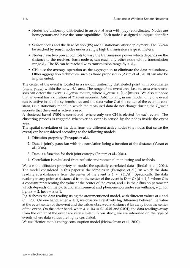
The center of the event is located in a random uniformly distributed point with coordinates(xevent, yevent) within the network’s area. The range of the event area, i.e., the area where sen-sors can detect the event is R_event meters, where R_event ∈ [1, A]meters. We also supposethat an event has a duration of T_event seconds. Additionally, in our model, only one eventcan be active inside the systemns area and the data value C at the center of the event is con-stant, i.e, a stationary model in which the measured data do not change during the T_eventseconds that the event is active is used.A clustered based WSN is considered, where only one CH is elected for each event. Theclustering process is triggered whenever an event is sensed by the nodes inside the eventarea.The spatial correlation of the data from the different active nodes (the nodes that sense theevent) can be considered according to the following models:
1. Diffusion propriety (Faruque, et al.).
2. Data is jointly gaussian with the correlation being a function of the distance (Vuran etal., 2006).
3. Data is a function for their joint entropy (Pattem et al., 2004).
4. Correlation is calculated from realistic environmental monitoring and testbeds.
We use the diffusion propriety to model the spatially correlated data (Jindal et al., 2004).The model considered in this paper is the same as in (Faruque, et al.) in which the datareading at a distance d from the center of the event is D ∝ f (1/d). Specifically, the datareading in any point at distance d from the center of the event is D = C/(d + 1)α, where C isa constant representing the value at the center of the event, and α is the diffusion parameterwhich depends on the particular environment and phenomenon under surveillance, e.g., forlight α = 2, heat = α ≃ 1.Fig. 8 shows the data reading using the aforementioned model, with different values of α andC = 250. On one hand, when α ≥ 1, we observe a relatively big difference between the valueat the event center of the event and the values observed at distance d far away from the centerof the event. On the other hand, when α < 1(α = 0.1, 0.01 and 0.001), the data readings awayfrom the center of the event are very similar. In our study, we are interested on the type ofevents where data values are highly correlated.We use Henizelman’s energy consumption model (Heinzelman et al., 2002).
0 20 40 60 80 1000
50
100
150
200
250
Dat
a re
adin
g R
distance
alpha=1alpha=0.1alpha=0.01alpha=0.001
www.intechopen.com
Energy Eficient Transmission Techniques in Continuous-Monitoring and Event-Detection Wireless Sensor Networks 117
0 20 40 60 80 1000
50
100
150
200
250
Dat
a re
adin
g R
distance
alpha=1alpha=0.1alpha=0.01alpha=0.001
Fig. 8. Variation of data reading with distance d from the center of the event.
6.2 Classical clustering protocol
A classical clustering process is composed by two phases: set up phase and steady state phase.When an event occurs in a random (uniformly distributed) point of the network, nodes insidethe event area weak up and start the clustering process. At the beginning of this phase, ac-tive nodes compete among each other to become CH. Specifically, active nodes transmit theircontrol packet to the BS according to the specified random medium access protocol. For thisprotocol the NP-CSMA control protocol is used since it has been proven to be the most energyefficient protocol. The control packet only comprises the node’s ID and no data are trans-mitted at this point. The first node that successfully transmits this packet becomes the CH.All nodes involved in the event reporting immediately send their signaling message to theBS. Therefore, the BS selects the first node that transmitted successfully the signaling messageand broadcasts a signaling message over the network for a CH notification. Thus the rest ofthe nodes inside the event area become CMs. In the steady phase, CMs send their data in ascheduled fashion using a Time Division Multiple Access (TDMA) protocol. The CH aggre-gates the data values received from its CMs with its own data and sends the resulted data tothe BS.
6.3 Proposed clustering protocol
The proposed clustering process is also composed of the same two phases, namely: set upphase and steady state phase. As in the classical protocol, the set up phase is triggered when-ever an event occurs in a region of the network. However, in the proposed scheme, the activenodes send their first measured data value to the BS, i.e., they no longer send just their controlpacket. Instead, active nodes send a data packet. The reason for this is that, this sensed data isused for the CH selection procedure. Indeed, this entails an extra energy consumption at theset up phase compared to the classical protocol. However, this first data transmission allowsimportant energy saving in the steady state phase.It is important to notice that, our proposed scheme is best suited for environments wherethe event conditions are fairly stable during the event duration. This is due to the fact thatthe CH is chosen according to the first sensed data. Hence, if the event conditions suffer ahigh variation, the originally selected CH may no longer render acceptable energy savings.Example of such applications includes fire surveillance forest, in which when a fire occurs in aregion, the temperature remains stationary for the duration of that fire in this region. Anotherexample of application includes target tracking. In this kind of application, the target is thesource of the measured data at sensor nodes, such as light or temperature. Here, the measureddata remains the same whenever the target stays in the same place and hence the sensor nodes
www.intechopen.com

Sustainable Wireless Sensor Networks118
sense the same measured data during the presence of the target. Next, we describe the set upand the steady phase of the proposed algorithm.
• In the set up phase, after reception of the first data packets of all active nodes, the BScalculates the difference between the data of node ni and the data of node nj (i �= j,and i ≤ N, j ≤ N). Next, these differences are summed over. We call this sum ofthe data value differences Si. Then, the BS selects as CH the node which minimizesthe total difference calculated value Si between each node ni and node nj (i �= j, andi ≤ N, j ≤ N). Finally, the BS broadcasts a control message to the active nodes to notifythe node selected as CH. Therefore, the rest of the nodes consider themselves as CMs.Note that there is no need for the CMs to send any extra packets since the BS alreadyknows the active nodes.
• In the steady state phase, CMs send the difference between their sensed data and theCH’s data value, which corresponds to a compressed value, called ∆i, rather than thecomplete data packet, value_CMi. Therefore, ∆i = |value_CMi − value_CH| representsthe difference between the i-th CM’s data value value_CMi, and the corresponding CHdata value value_CH. In order to perform this compression, the CH sends its completesample data value to the CMs at the beginning of each round. Therefore, the CMssend only the ∆i to the CH. The main advantage of the proposal scheme is that the Si
calculation is centralized at the BS, which is not energy constrained.
6.4 Mathematical Model
In this section, the mathematical model for the clustering protocol is described. For reasonsof clarity, the random access protocol is not considered in this analysis. First, because it hasbeen studied in detail in the previous sections. Second, because we are interested on studyingthe effect of the compression scheme without the extra energy consumption of the collisionsand idle listening and third, because the effect of the energy consumption is considered in thesimulation results.The total energy consumed in the network Etotal for a duration of the event can be calculatedas follows:
Etotal = Ecompeting + Ereporting (26)
where Ecompeting is the energy consumed during the cluster formation phase and Ereporting isthe energy consumed during the steady state phase. We calculate hereafter E[Etotal ], the av-erage energy consumed through the network for both the classical and the proposed protocolas E[Etotal ] = E[Ecompeting] + E[Ereporting].
6.4.1 Classical protocol
We first calculate E[Ecompeting]. The energy consumed at the cluster formation phase is due tothe signaling packet transmission of the active nodes in the event area directly to the BS plusthe reception of the signaling packet from the BS to the active nodes, then:
E[Ecompeting] = m × [Etx(S, Rt) + Erx(S)] (27)
where m = Nπ(R_event)2/A2, is the average number of active nodes in the dish of radiusR_event and N is the total number of nodes in the network. S = 24bit is the size of signalingmessage, m × Etx(S, Rt) is the energy consumed to sent by the m compete messages to the BS,
www.intechopen.com
Energy Eficient Transmission Techniques in Continuous-Monitoring and Event-Detection Wireless Sensor Networks 119
and m × Erx(S) is the energy consumed by the resulting compete message sent from the BSthought the network. On the other hand, the average energy consumption in the steady phaseper event can be calculated as:
E[Ereporting] = Number_report × [Etx(S, Rc)+ (m − 1)× Erx(S)+
(m − 1)× Etx( f ixe, Rc)+ (m − 1) ∗ Erx( f ixe)+ EDA × f ixe + Etx( f ixe, Rt)]
where fixe is the size of the full data packets of 32bits, Number_report = 29 is the number ofpacket sent during the steady phase, Etx(S, Rc) is the energy consumed due to the signalingmessages sent by the CH to its CMs to begin the event reporting, (m− 1)× Erx(S) is the energyconsumed by CMs to receive this message, (m − 1)× Etx( f ixe, Rc) is the energy consumed bythe CMs to send the data to the CH, (m − 1)× Erx( f ixe) is the energy consumed by the CHto receive the data sent by the CMs, EDA × f ixe is the energy consumed by the CH due to thedata aggregation, and Etx( f ixe, Rt) is the energy consumed by the CH to send the aggregateddata to the BS
6.4.2 Proposed protocol
Note that, at the cluster formation phase, the proposed scheme behaves in the same manneras the classical protocol with the important difference that the nodes transmit the data packetinstead of the signaling packet, then:
E[Ecompeting] = m × [Etx( f ixe, Rt)+ Erx(S)] (28)
where m × Etx( f ixe, Rt) is the energy consumed to send the m data packets to the BS andm × Erx(S) is the energy consumed by the transmission of the compete packets from the BS tothe active nodes in the network. The energy consumption in the steady state can be found asfollows:
E[Ereporting] = Etx( f ixe, Rc)+ (m − 1)Erx( f ixe)+ Number_report[Etx(S, Rc)+ (m − 1)Erx(S)+
(m − 1)Etx(S + log2(E[∆i]), Rc + (m − 1)Erx(S + log2(E[∆i]))+ f ixeEDA + Etx( f ixe, Rt)])
where, Etx( f ixe, Rc) is the energy consumed by the data packet transmission that is used asthe reference value from the CH to the CMs, (m − 1)× Erx( f ixe) is the energy consumed bythe CMs to receive the aforementioned reference value, Etx(S, Rc) is the energy consumedfrom a signaling message sent by the CH to its CMs in order to send their data, (m − 1) ×Erx(S) is the energy consumed by CMs to receive this signaling message, (m − 1)× Etx(S +log2(E[∆i]), Rc) is the energy consumed by the CMs to send the compressed data to the CH,(m − 1)× Erx(S + log2(E[∆i])) is the energy consumed by the CH to receive the compresseddata from the CMs, EDA × f ixe is the energy consumed by the CH due to the data aggregationprocedure, Etx( f ixe, Rt) is the energy consumed by the CH to send the aggregated data to theBS, E[∆i] is the average data packet size which corresponds to the difference between theCMs’ data and the CH’s data. It is worth noting that considering a uniform node distributionwith a large N, the node that minimizes the distance in the R_event region will be located inthe center of R_event. Therefore, to calculate E[∆i] let us first calculate the average distancebetween active nodes and the CH, E[dtoCH ].
∫ R_event0 r2πrdr/
∫ R_event0 2πrdr = 2R_event/3
www.intechopen.com
Sustainable Wireless Sensor Networks120
If the density of the nodes is uniform through the R_event area. We now calculate E[∆i]. Theaverage data difference between the data at the CM and the reference value at the CH C isdescribed by:
E[∆i] = C
∣
∣
∣
∣
1 −1
(1 + 2R_event/3)α
∣
∣
∣
∣
(29)
6.5 Numerical Results
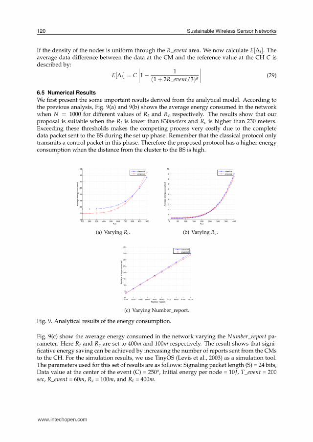
We first present the some important results derived from the analytical model. According tothe previous analysis, Fig. 9(a) and 9(b) shows the average energy consumed in the networkwhen N = 1000 for different values of Rt and Rc respectively. The results show that ourproposal is suitable when the Rt is lower than 830meters and Rc is higher than 230 meters.Exceeding these thresholds makes the competing process very costly due to the completedata packet sent to the BS during the set up phase. Remember that the classical protocol onlytransmits a control packet in this phase. Therefore the proposed protocol has a higher energyconsumption when the distance from the cluster to the BS is high.
100 200 300 400 500 600 700 800 900 100018
20
22
24
26
28
30
32
34
R_t
Ave
rage
ene
rgy
cons
umed
classicalproposal
(a) Varying Rt.
0 50 100 150 200 250 300 350 4000
1
2
3
4
5
6
7
8
9
10
R_c
Ave
rage
ene
rgy
cons
umed
classicalproposal
(b) Varying Rc.
1000 2000 3000 4000 5000 6000 7000 8000 9000 100000
5
10
15
20
25
30
35
40
Number_repport
Ave
rage
ene
rgy
cons
umed
classicalproposal
(c) Varying Number_report.
Fig. 9. Analytical results of the energy consumption.
Fig. 9(c) show the average energy consumed in the network varying the Number_report pa-rameter. Here Rt and Rc are set to 400m and 100m respectively. The result shows that signi-ficative energy saving can be achieved by increasing the number of reports sent from the CMsto the CH. For the simulation results, we use TinyOS (Levis et al., 2003) as a simulation tool.The parameters used for this set of results are as follows: Signaling packet length (S) = 24 bits,Data value at the center of the event (C) = 250°, Initial energy per node = 10J, T_event = 200sec, R_event = 60m, Rc = 100m, and Rt = 400m.
0 5 10 15 200
0.1
0.2
0.3
0.4
0.5
0.6
0.7
0.8
0.9
1
Time= number of events
Rat
io o
f the
ene
rgy
cons
umed
.
Ratio: proposal/classicalRatio: proposal/single hop.
www.intechopen.com
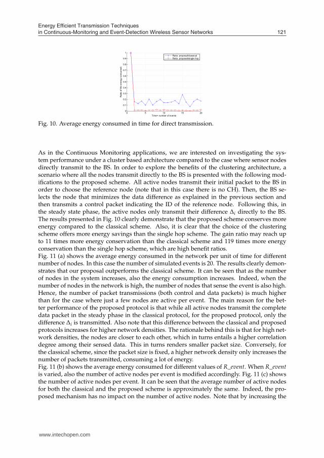
Energy Eficient Transmission Techniques in Continuous-Monitoring and Event-Detection Wireless Sensor Networks 121
100 200 300 400 500 600 700 800 900 100018
20
22
24
26
28
30
32
34
R_t
Ave
rage
ene
rgy
cons
umed
classicalproposal
0 50 100 150 200 250 300 350 4000
1
2
3
4
5
6
7
8
9
10
R_c
Ave
rage
ene
rgy
cons
umed
classicalproposal
1000 2000 3000 4000 5000 6000 7000 8000 9000 100000
5
10
15
20
25
30
35
40
Number_repport
Ave
rage
ene
rgy
cons
umed
classicalproposal
0 5 10 15 200
0.1
0.2
0.3
0.4
0.5
0.6
0.7
0.8
0.9
1
Time= number of events
Rat
io o
f the
ene
rgy
cons
umed
.
Ratio: proposal/classicalRatio: proposal/single hop.
Fig. 10. Average energy consumed in time for direct transmission.
As in the Continuous Monitoring applications, we are interested on investigating the sys-tem performance under a cluster based architecture compared to the case where sensor nodesdirectly transmit to the BS. In order to explore the benefits of the clustering architecture, ascenario where all the nodes transmit directly to the BS is presented with the following mod-ifications to the proposed scheme. All active nodes transmit their initial packet to the BS inorder to choose the reference node (note that in this case there is no CH). Then, the BS se-lects the node that minimizes the data difference as explained in the previous section andthen transmits a control packet indicating the ID of the reference node. Following this, inthe steady state phase, the active nodes only transmit their difference ∆i directly to the BS.The results presented in Fig. 10 clearly demonstrate that the proposed scheme conserves moreenergy compared to the classical scheme. Also, it is clear that the choice of the clusteringscheme offers more energy savings than the single hop scheme. The gain ratio may reach upto 11 times more energy conservation than the classical scheme and 119 times more energyconservation than the single hop scheme, which are high benefit ratios.Fig. 11 (a) shows the average energy consumed in the network per unit of time for differentnumber of nodes. In this case the number of simulated events is 20. The results clearly demon-strates that our proposal outperforms the classical scheme. It can be seen that as the numberof nodes in the system increases, also the energy consumption increases. Indeed, when thenumber of nodes in the network is high, the number of nodes that sense the event is also high.Hence, the number of packet transmissions (both control and data packets) is much higherthan for the case where just a few nodes are active per event. The main reason for the bet-ter performance of the proposed protocol is that while all active nodes transmit the completedata packet in the steady phase in the classical protocol, for the proposed protocol, only thedifference ∆i is transmitted. Also note that this difference between the classical and proposedprotocols increases for higher network densities. The rationale behind this is that for high net-work densities, the nodes are closer to each other, which in turns entails a higher correlationdegree among their sensed data. This in turns renders smaller packet size. Conversely, forthe classical scheme, since the packet size is fixed, a higher network density only increases thenumber of packets transmitted, consuming a lot of energy.Fig. 11 (b) shows the average energy consumed for different values of R_event. When R_event
is varied, also the number of active nodes per event is modified accordingly. Fig. 11 (c) showsthe number of active nodes per event. It can be seen that the average number of active nodesfor both the classical and the proposed scheme is approximately the same. Indeed, the pro-posed mechanism has no impact on the number of active nodes. Note that by increasing the
www.intechopen.com

Sustainable Wireless Sensor Networks122
10 20 30 40 50 60 700
0.2
0.4
0.6
0.8
1
1.2
1.4
# Number of nodes.
Tota
l ene
rgy
cons
umed
in th
e ne
twor
k (J
oule
/tim
es). standard
proposal
(a) Average energy consumption forunit of time vs number of nodes
0 5 10 15 200
0.005
0.01
0.015
0.02
0.025
0.03
Time= number of rounds
Ave
rage
con
sum
ed e
nerg
y (J
oule
s/no
de)
S.R_event=30S.R_event=60S.R_event=90P.R_vent=30P.R_event=60P.R_event=90
(b) Average energy consumed withvarying the R_event region
0 2 4 6 8 10 12 14 16 18 200
5
10
15
20
25
30
35
40
45
50
Time= number of rounds
Num
ber o
f par
ticip
ant
P.R_event=30P.R_event=60P.R_event=90S.R_event=30S.R_event=60S.R_event=90
(c) Number of active nodes for eachround
0 5 10 15 200
0.005
0.01
0.015
0.02
0.025
0.03
0.035
0.04
Time= number of rounds
Ave
rage
ene
rgy
cons
umed
(Jou
les/
node
)
S.T_event=200S.T_event=300S.T_event=400P.T_event=200P.T_event=300P.T_event==400
(d) Average energy consumption vsT_event
Fig. 11. Average energy consumption for unit of time for different parameters.
number of active nodes the energy consumption also increases. Observe for instance that theenergy consumption when R_event = 30 is less than the consumption when R_event = 60 and90. In each scenario, we observe that enabling our compression scheme reduces the energyconsumption over the network and therefore extends the network lifetime.Fig. 11 (c) shows the average energy consumed for different values of the T_event period.Increasing T_event also increases the period of the steady state phase and the number of datareported, therefore it can be seen an increase on the energy consumption. That explains whythe energy consumed for T_event = 200 sec is less than the energy consumed for T_event =300 and 400 sec. In each scenario, we observe that enabling our compression scheme reducesthe energy consumption over the network and therefore extends the network lifetime. It isimportant to note that the proposed mechanism is particularly energy efficient for high eventduration times. This is due to the fact that as the event duration increases, the CMs in theclassical scheme transmit many full length packets while for the proposed mechanism, theCMs also transmit many packets but with a much smaller length. This renders a slight increaseof energy consumption for the proposed mechanism while for the classical scheme there is animportant augmentation in the energy consumption when the event duration increases.
www.intechopen.com
Energy Eficient Transmission Techniques in Continuous-Monitoring and Event-Detection Wireless Sensor Networks 123
10 20 30 40 50 60 700
0.2
0.4
0.6
0.8
1
1.2
1.4
# Number of nodes.
Tota
l ene
rgy
cons
umed
in th
e ne
twor
k (J
oule
/tim
es). standard
proposal
0 5 10 15 200
0.005
0.01
0.015
0.02
0.025
0.03
Time= number of rounds
Ave
rage
con
sum
ed e
nerg
y (J
oule
s/no
de)
S.R_event=30S.R_event=60S.R_event=90P.R_vent=30P.R_event=60P.R_event=90
0 2 4 6 8 10 12 14 16 18 200
5
10
15
20
25
30
35
40
45
50
Time= number of rounds
Num
ber o
f par
ticip
ant
P.R_event=30P.R_event=60P.R_event=90S.R_event=30S.R_event=60S.R_event=90
0 5 10 15 200
0.005
0.01
0.015
0.02
0.025
0.03
0.035
0.04
Time= number of rounds
Ave
rage
ene
rgy
cons
umed
(Jou
les/
node
)
S.T_event=200S.T_event=300S.T_event=400P.T_event=200P.T_event=300P.T_event==400
7. Conclusion
This work has focused on studying the benefits to the energy consumption that can be gainedby adding CM-EDR capabilities to systems of classical, unscheduled and cluster-based WSNs.The resulting continuous-monitoring WSN has been modeled, analyzed, simulated and stud-ied.It has been verified that CM-EDR can allow for an improvement in the network lifetime whileensuring the continuous-monitoring task. More significantly however, it has been shownthat for calm supervised environment, it is more convenient to use the optional OCM-EDR,whereas in agitated environment, it is better to use the basic CM-EDR mechanism.It is worth noting that enabling the CM-EDR and OCM-EDR mechanisms reduces always theenergy consumption. On the other hand, the OCM-EDR mechanism has superior performancein terms of energy consumption for low values of λ while for higher values of λ the CM-EDRmechanism provides lower energy consumption.For both low and moderate values of λ, with low or high values of Nidle, OCM-EDR providesgood performance. Considering moderate values of Nidle the performance is superior sincethe energy consumption decreases. A similar effect can be seen when Nsleep is varied. In thiscase, OCM-EDR has the best performance when λ is low. On the other hand, when the valueof λ is high, OCM-EDR presents relatively bad performance for any values of Nidle and Nsleep
since the energy consumption is higher than the basic CM-EDR mechanism.For the event detection applications, a new cluster-based compression technique has beenproposed. The clustering scheme is based on selecting the node that reduces the packet sizeamong all active nodes in the system. The BS selects the node which minimizes the totalamount of data as a CH, therefore it increases the efficiency of the compression technique bysending only the difference, rather than the complete data value to the CH. By varying differ-ent parameters of the system, simulation and analytical results conclude that considering thespatial correlation in the communication of WSNs achieves significant energy conservationcompared to a classical clustering scheme. The ratio benefit may reach up to 11 times the clas-sical scheme. The proposed scheme extends the network lifetime. In addition, an approximatemathematical model is developed which validate the results.
8. References
K. Kredo II, P. Mohapatra, Medium access control in wireless sensor networks, Computer Net-works, Volume 51, Issue 4, 14, pp. 961–994, March 2007.
W. B. Heinzelman, A. P. Chandrakasan, H. Balakrishnan, An application-specific protocol architec-ture for wireless microsensor networks, IEEE Transactions on Wireless Communication,vol. 1, no. 4, pp. 660–670, Oct. 2002.
Wireless LAN Medium Access Control (MAC) and Physical Layer (PHY) Specifications, ISO/IECIEEE 802.11 Standard, 1999.
B. Sericola, Closed form solution for the distribution of the total time spent in a subset of states of aMarkov process during a finite observation period, Journal of Applied Probability, 27, pp.713–719, 1990.
N. Bouabdallah, M. Rivero-Angeles, B. Sericola, Continuous monitoring using event-drivenreporting for cluster-based wireless sensor networks, IEEE Transactions on VehicularTechnology, vol. 58, No. 7, pp. 3360-3479, Sep. 2007.
www.intechopen.com

Sustainable Wireless Sensor Networks124
C. Intanagonwiwat, R. Govindan, and D. Estrin, Directed Diffusion: A Scalable and Robust Com-munication Paradigm for Sensor Networks, (2000), in Proc. Sixth Annual InternationalConference on Mobile Computing and Networks (MobiCom 2000), Boston, Mas-sachusetts, August 2000.
M. Larrea, C. Martin, J. J. Astrain, Hierarchical and fault-tolerant data aggregation in wireless sen-sor networks, in Proc. IEEE Second International Symposium on Wireless PervasiveComputing (ISWPC ’07), pp. 531–536, Feb. 2007.
F. Bouabdallah, N. Bouabdallah, and R. Boutaba, Towards Reliable and Efficient Reporting inWireless Sensor Networks, IEEE Transaction on Mobile Computing, 2009.
M. C. Vuran, and I. F. Akyildiz, Spatial correlation-based collaborative medium access control inwireless sensor networks, IEEE/ACM Transactions On Networking, vol 14, Issue 2, pp.316–329, April 2006.
A. Woo, D.E. Culler, A transmission control scheme for media access in sensor networks, in Proc.of the International Conference on Mobile Computing and Networking (MobiCom2001), pp. 221–235, 2001.
M. A.l Azim, S. Moad and N. Bouabdallah, SAG: Smart Aggregation Technique for Continuous-Monitoring in Wireless Sensor Networks, In Proc. of the IEEE International Comunica-tion Conference (ICC), Cap town, May 2010.
J. Faruque and A. Helmy, Rugged: Routing on fingerprint gradient in sensor network, in IEEEinternational confrenece on pervasive Service (ICPS’2004), July 2004.
S. Pattem, B. Krishnmachari, R. Govindan and J. Heidemann, The impact of spatial correlationon routing with coprerssion in wireless sensor networks, in Synposium on informationPorcessin in Sensor Networks," (IPSN), April 2004.
A. Jindal and K. Psounis,‘Modeling spatially-correlated sensor network data, In the Proceedingsof IEEE International Conference on Sensor and Ad hoc Communications and Net-works (SECON’04), Santa Clara, CA, October 2004.
P. Levis, N. Lee, M. Welsh and D. Culler, TOSSIM: Accurate and Scalable Simulation of EntireTinyOS Applications, In Proc. of the First ACM Conference on Embedded NetworkedSensor Systems (SenSys), 2003.
www.intechopen.com
Sustainable Wireless Sensor NetworksEdited by Yen Kheng Tan
ISBN 978-953-307-297-5Hard cover, 574 pagesPublisher InTechPublished online 14, December, 2010Published in print edition December, 2010
InTech EuropeUniversity Campus STeP Ri Slavka Krautzeka 83/A 51000 Rijeka, Croatia Phone: +385 (51) 770 447 Fax: +385 (51) 686 166www.intechopen.com
InTech ChinaUnit 405, Office Block, Hotel Equatorial Shanghai No.65, Yan An Road (West), Shanghai, 200040, China
Phone: +86-21-62489820 Fax: +86-21-62489821
Wireless Sensor Networks came into prominence around the start of this millennium motivated by theomnipresent scenario of small-sized sensors with limited power deployed in large numbers over an area tomonitor different phenomenon. The sole motivation of a large portion of research efforts has been to maximizethe lifetime of the network, where network lifetime is typically measured from the instant of deployment to thepoint when one of the nodes has expended its limited power source and becomes in-operational –commonly referred as first node failure. Over the years, research has increasingly adopted ideas from wirelesscommunications as well as embedded systems development in order to move this technology closer to realisticdeployment scenarios. In such a rich research area as wireless sensor networks, it is difficult if not impossibleto provide a comprehensive coverage of all relevant aspects. In this book, we hope to give the reader with asnapshot of some aspects of wireless sensor networks research that provides both a high level overview aswell as detailed discussion on specific areas.
How to referenceIn order to correctly reference this scholarly work, feel free to copy and paste the following:
Nizar Bouabdallah, Mario E. Rivero-angeles, Sofiane Moad and Bruno Sericola (2010). Energy EfficientTransmission Techniques in Continuous-Monitoring and Event-Detection Wireless Sensor Networks,Sustainable Wireless Sensor Networks, Yen Kheng Tan (Ed.), ISBN: 978-953-307-297-5, InTech, Availablefrom: http://www.intechopen.com/books/sustainable-wireless-sensor-networks/energy-efficient-transmission-techniques-in-continuous-monitoring-and-event-detection-wireless-senso

© 2010 The Author(s). Licensee IntechOpen. This chapter is distributedunder the terms of the Creative Commons Attribution-NonCommercial-ShareAlike-3.0 License, which permits use, distribution and reproduction fornon-commercial purposes, provided the original is properly cited andderivative works building on this content are distributed under the samelicense.