energy efficiency in the south · energy efficiency in the south ... calculator” that contributed...
TRANSCRIPT
ENERGY EFFICIENCY IN THE SOUTH
Marilyn A. Brown,1 Etan Gumerman,2
Xiaojing Sun,2 Youngsun Baek,1 Joy Wang,1 Rodrigo Cortes,1
and Diran Soumonni1
April 12, 2010
Sponsored by:
Energy Foundation
Kresge Foudation
Turner Foundation
Published by:
Southeast Energy Efficiency Alliance
Atlanta, GA
1Georgia Institute of Technology 2Duke University
ACKNOWLEDGEMENTS
Funding for this research was provided by the Energy Foundation (under the direction of
Meredith Wingate), the Turner Foundation (under the direction of Judy Adler), and the Kresge
Foundation (under the direction of Lois Debacker). The support of these three sponsors is greatly
appreciated.
Several Graduate Research Assistants contributed meaningfully to the completion of this report.
At the Georgia Institute of Technology, Ben Deitchman assisted with the analysis of employment
and water conservation impacts of energy efficiency investments, Yu Wang assisted with the
residential sector NEMS analysis, and Elizabeth Noll helped with the graphics. At Duke
University, Cullen Morris helped with the commercial sector NEMS analysis and Gabriel Kwok
helped with the final report preparation. Their assistance is also appreciated.
Skip Laitner (American Council for an Energy Efficient Economy) developed the “jobs
calculator” that contributed to our estimates of employment and economic impacts of the energy-
efficiency policies examined in this study.
Michael Halicki (Ahmann, Inc.) and Ben Taube and Julie Harrison (Southeast Energy Efficiency
Alliance) helped the team summarize the report‟s findings in terms that could be easily digested
and understood by a wide range of audiences.
Valuable comments on a previous draft of this report were received from Paul Baer (Georgia
Institute of Technology), Stan Hadley (Oak Ridge National Laboratory), John Wilson (Southern
Alliance for Clean Energy), and Todd Wooten (Duke University)
Useful feedback regarding the study‟s design and results was also provided by members of the
project‟s advisory and stakeholder committees, composed of:
Dennis Creech (Southface Institute)
Larry Shirley (North Carolina Department of Commerce)
Dan Skelly (U.S. Energy Information Agency)
William “Dub” Taylor (Texas State Energy Conservation Office)
Stephen Walz (Commonwealth of Virginia)
Chris Edge, Progress Energy
John Masiello, Progress Energy
Robert Burnette, Dominion Power
Raiford Smith, Duke Energy
The authors are grateful for the willingness of these individuals to engage in a dialogue about the
potential to expand energy-efficiency resources in the South. Any errors that survived this review
process are strictly the responsibility of the authors.

Contents ENERGY EFFICIENCY IN THE SOUTH ......................................................................................... i
ACKNOWLEDGEMENTS ......................................................................................................... ii
EXECUTIVE SUMMARY ........................................................................................................... vi
Magnitude of the Energy-Efficiency Resource in the South ................................................... viii
Impact on Power Plant Construction ......................................................................................... xi
Economic Impacts ..................................................................................................................... xii
Cost-Effectiveness of the Portfolio of Energy-Efficiency Policies ......................................... xiv
Water Conservation from Energy Efficiency ........................................................................... xv
Policy Supply Curves for Energy Efficiency in the South ...................................................... xvi
Carbon Constrained Sensitivity Analysis ............................................................................... xvii
Conclusions ............................................................................................................................ xviii
1. INTRODUCTION .................................................................................................................. 2
1.1 GOALS AND ORGANIZATION OF THE REPORT .................................................... 2
1.2 OVERVIEW OF THE SOUTH CENSUS REGION ....................................................... 4
1.3 ENERGY SUPPLY IN THE SOUTH ............................................................................. 5
1.4 ENERGY USE IN THE SOUTH ..................................................................................... 5
1.4.1 Energy Consumption by Source ............................................................................... 6
1.4.2 Energy Consumption by Sector ................................................................................ 8
1.4.3 Energy Prices ............................................................................................................ 9
1.4.4 Carbon Footprint ..................................................................................................... 10
1.5 ENERGY-EFFICIENCY PROGRAMS AND PRACTICES IN THE SOUTH ............ 10
1.5.1 Illustrative Energy-Efficient Technologies and Policies ........................................ 10
1.5.2 Energy-Efficiency Practices in the South ............................................................... 12
1.5.3 Previous Estimates of Energy-Efficiency Potential in the South ............................ 15
2. METHODOLOGY .................................................................................................................. 18
2.1 PORTFOLIO OF ENERGY-EFFICIENCY POLICIES ............................................... 20
2.2 NATIONAL ENERGY MODELING SYSTEM (NEMS) ............................................ 21
2.2.1 The Baseline Forecast ............................................................................................. 22
2.3 DEFINITION OF PROGRAM ACHIEVABLE POTENTIAL ..................................... 23
2.3.1 Cost-Effectiveness Tests ......................................................................................... 24
2.3.2 Measuring Energy Savings: Delivered and Primary ............................................... 25
2.4 RESULTS...................................................................................................................... 25
2.5 SENSITIVITY ANALYSIS CASE: CARBON CONSTRAINED FUTURE ............... 26

2.6 ESTIMATING GRP AND EMPLOYMENT IMPACTS .............................................. 27
2.7 CALCULATING WATER CONSERVATION FROM ENERGY EFFICIENCY ...... 27
2.8 METHOD FOR DERIVING STATE-SPECIFIC ESTIMATES ................................... 28
3. ENERGY EFFICIENCY IN RESIDENTIAL BUILDINGS ................................................... 29
3.1 INTRODUCTION TO THE RESIDENTIAL BUILDINGS IN THE SOUTH ............. 29
3.2 BARRIERS TO RESIDENTIAL ENERGY EFICIENCY AND POLICY OPTIONS . 30
3.3 ENERGY EFFICIENCY POLICIES IN RESIDENTIAL BUILDINGS ...................... 34
3.3.1 Residential Building Codes with Third-Party Verification ................................... 34
3.3.2 Appliance Incentives and Standards ....................................................................... 39
3.3.3 Expanded Low-Income Weatherization Assistance ............................................... 45
3.3.4 Residential Retrofit Incentive with Equipment Standards ...................................... 53
3.4 INTEGRATED RESIDENTIAL POLICIES ................................................................ 58
3.5 SUMMARY AND DISCUSSION OF RESULTS FOR THE RESIDENTIAL SECTOR 63
3.5.1 Comparison with Other Studies .............................................................................. 63
3.5.2 Limitations and Needs for Future Research............................................................ 64
4. ENERGY EFFICIENCY IN THE COMMERCIAL SECTOR ................................................ 67
4.1 INTRODUCTION TO COMMERCIAL BUILDINGS IN THE SOUTH .................... 67
4.2 BARRIERS TO COMMERCIAL ENERGY EFICIENCY AND POLICY OPTIONS 69
4.2.1 Barriers to Energy-Efficiency in Commercial Buildings........................................ 69
4.2.2 Policy Options to Improve Energy-Efficiency in the Commercial Sector ............. 69
4.3 MODELED ENERGY EFFICIENCY POLICIES FOR COMMERCIAL SECTOR ... 73
4.3.1 Commercial Appliance Standards .......................................................................... 73
4.3.2 Commercial Building HVAC Retrofit .................................................................... 79
4.4 COMBINED COMMERCIAL POLICIES, RESULTS ................................................ 83
4.4.1 Energy Efficiency .................................................................................................. 83
4.4.2 Energy Bill Savings ............................................................................................... 85
4.4.3 Economic Test of Combined Commercial Policies ................................................ 86
4.5 SUMMARY AND DISCUSSION OF RESULTS FOR COMMERCIAL SECTOR ... 86
4.5.1 Comparison with Other Studies .............................................................................. 88
4.5.2 Limitations and Needs for Future Research............................................................ 89
5. ENERGY EFFICIENCY IN INDUSTRY ................................................................................ 92
5.1 INTRODUCTION TO THE INDUSTRIAL SECTOR IN THE SOUTH .................... 92
5.2 POLICY OPTIONS FOR INDUSTRIAL ENERGY EFFICIENCY ............................ 93
5.2.1 Barriers to Industrial Energy Efficiency in the South ............................................. 93

5.2.2 Policy Options ......................................................................................................... 95
5.3 ENERGY EFFICIENCY POTENTIAL IN INDUSTRY IN THE SOUTH .................. 97
5.3.1 Spreadsheet Analysis for Industrial Assessments for Plant Utility Upgrades ........ 97
5.3.2 SNUG-NEMS Modeling of Industrial Assessments of Plant Utility Upgrades ... 100
5.3.3 Policies to Accelerate Industrial Process Improvements ...................................... 103
5.3.4 SNUG-NEMS Modeling to Accelerate Industrial Process Improvements ........... 106
5.3.5 Supporting Industrial Combined Heat and Power (CHP) with Incentives ........... 108
5.3.6 SNUG-NEMS Modeling of Industrial CHP with Incentives ................................ 111
5.4 COMBINED INDUSTRIAL ENERGY EFFICIENCY POLICIES ............................ 116
5.4.1 Energy Efficiency Results..................................................................................... 116
5.4.2. Energy Price Results ............................................................................................. 117
5.4.3 Energy Bill Savings .............................................................................................. 118
5.5 SUMMARY OF RESULTS FOR INDUSTRIAL ENERGY EFFICIENCY .............. 119
5.5.1 Comparison with Other Studies ................................................................................. 120
5.5.2 Limitations and the Need for Further Research ......................................................... 121
6. INTEGRATED ANALYSIS .................................................................................................. 123
6.1 INTRODUCTION ....................................................................................................... 123
6.2 ENERGY-EFFICIENCY POLICY SCENARIO RESULTS ................................... 124
6.2.1 Energy Savings and Efficiency ............................................................................. 124
6.2.2 Electricity Capacity ............................................................................................... 126
6.2.3 Rate Impact ........................................................................................................... 128
6.2.4 Energy Bill Savings ............................................................................................. 128
6.2.5 Economic Tests and Supply Curves ..................................................................... 129
6.2.6 Macroeconomic and Job Impacts......................................................................... 133
6.3 SENSITIVITY ANALYSIS ............................................................................................ 137
6.3.1 Elements of the CCF Sensitivity ........................................................................... 138
6.3.2 Energy-Efficiency Policies and CCF .................................................................... 140
6.4 WATER CONSERVATION THROUGH ENERGY EFFICIENCY ............................. 144
6.4.1 Water in Reference Future .................................................................................... 144
6.4.2 Water Conservation from the Energy-Efficiency Policies .................................... 145
6.4.3 Water Conservation in the Carbon Constrained Future ........................................ 146
6.5 CONCLUSIONS.............................................................................................................. 148
References ................................................................................................................................... 151

vi
EXECUTIVE SUMMARY
The economic recession, climate change concerns and rising electricity costs have motivated
many states to embrace energy efficiency as a way to create new local jobs, lower energy bills,
and promote environmental sustainability. With this surge of interest in energy efficiency,
policymakers are asking how much wasted energy can be eliminated by expanding investments
in cost-effective technologies and practices.
This report describes the results of primary in-depth research focused on the size of the South‟s
energy-efficiency resources and the types of policies that could convert this potential resource
into reality over the next 20 years. We limit the scope of our analysis to energy-efficiency
improvements in three sectors: residential and commercial buildings and industry (RCI). Our
rigorous modeling approach – applied uniformly across the multi-state region and accompanied
by a detailed documentation of assumptions and methods – separates this study from many
previous assessments of energy-efficiency potential.
The major findings are listed below.
1. Aggressive energy-efficiency initiatives in the South could prevent energy
consumption in the RCI sectors from growing over the next twenty years.
The initiatives would involve actions at multiple levels (state and local, national,
utility, business, and personal). In the absence of such initiatives, energy consumption
in these three sectors is forecast to grow by approximately 16% between 2010 and
2030.
2. Fewer new power plants would be needed with a commitment to energy
efficiency.
Our analysis of nine illustrative policies shows the ability to retire almost 25 GW of
older power plants – approximately 10 GW more than in the reference case. The nine
policies would also avoid over the next twenty years the need to construct 49 GW of
new plants to meet a growing electricity demand from the RCI sectors.
3. Increased investments in cost-effective energy efficiency would generate jobs and
cut utility bills.
The public and private investments stimulated by the nine energy-efficiency policies
would deliver rapid and substantial benefits to the region. In 2020, energy bills in the
South would be reduced by $41 billion, electricity rate increases would be moderated,
380,000 new jobs would be created, and the region‟s economy would grow by $1.23
billion.
The cost/benefit ratios for the modeled policies range from 4.6 to 0.3, with only two
showing costs greater than benefits. When the value of saved CO2 is included, only
one policy is not cost effective, and it could be tailored to reduce the amount of
subsidy.

vii
4. Energy efficiency would result in significant water savings.
The electricity generation that could be avoided by the nine energy-efficiency policies
in the South could in turn conserve significant quantities of freshwater consumed for
cooling. In the North American Electric Reliability Council (NERC) regions in the
South, 8.6 billion gallons of freshwater could be conserved in 2020 (56% of projected
growth in cooling water needs) and in 2030 this could grow to 20.1 billion gallons of
conserved water (or 45% of projected growth).
Methodology and Background
The research team used a modified version of the National Energy Modeling System (NEMS) for
its analysis, which is referred to as “SNUG-NEMS” (SNUG is short for the Southeast NEMS
Users Group). By employing a hybrid approach using both the “bottom-up” and “top-down”
modeling features of SNUG-NEMS and Global Insight‟s macroeconomic model, we are able to
characterize a host of complicated interactive effects that are important, but often overlooked
consequences of energy and climate policies. These include:
the interaction of multiple energy efficiency policies on one another and their effect on
the final demand for energy;
the interaction of demand-side policies on supply-side trends;
the feedback of energy efficiency policies on energy prices, and the subsequent (i.e.,
second-order) effect of prices on energy demand; and
the interaction of energy-efficiency policies with the implementation of a carbon
constrained future that puts a price on carbon.
We do not examine the impact of energy-efficiency investments on peak demand reductions.
While clipping system peaks is critical to improving electric system performance, we treat this as
an ancillary benefit of energy efficiency. Nor do we examine the role of demand-response or
load-management programs aimed strictly at shifting on-peak consumption to off-peak hours.
The geographic scope covered by this report is defined by the U.S. Census Bureau‟s definition of
the South, composed of the District of Columbia and 16 States stretching from Delaware down
the Appalachian Mountains, including the Southern Atlantic seaboard and spanning the Gulf
Coast to Texas. The South is the largest and fastest growing region in the United States, with
36% of the nation‟s population and a considerably larger share of the nation‟s total energy
consumption (44%) and supply (48%). It produces a large portion of the nation‟s fossil fuels, and
the vast majority of the energy it consumes is derived from fossil resources.
Relative to the rest of the country, the South consumes a particularly large share of industrial
energy, accounting for 51% of the nation‟s total industrial energy use. In addition, the region has
a higher-than-average per capita energy consumption for each of the end-use sectors covered in

viii
this report: the South consumes 43% of the nation‟s electric power, 40% of the energy consumed
in residences, and 38% of the energy used in commercial buildings. This energy-intensive
lifestyle may be influenced by a range of factors including:
the South‟s historically low electricity rates,
the significant heating and cooling loads that characterize many southern states,
its relatively weak energy conservation ethic (based on public opinion polls),
its low market penetration of energy-efficient products (based on purchase behavior) and
its lower than average expenditures on energy-efficiency programs.
If the South could achieve the substantial energy-efficiency improvements that have already been
proven effective in other regions and other nations, carbon emissions across the South would
decline, air quality would improve, and plans for building new power plants to meet growing
electricity demand could be downsized and postponed, while saving ratepayers money.
Magnitude of the Energy-Efficiency Resource in the South
The U.S. Energy Information Administration projects energy consumption in the RCI sectors of
the South to increase over the next 20 years, expanding from approximately 30,000 TBtu in 2010
to more than 35,000 TBtu in 2030 (Figure ES.1).
Figure ES.1 Primary Energy Consumption Projections (RCI Sectors) in the South
With the nine energy-efficiency policies, energy consumption does not grow over the next 20
years. This flat consumption trajectory represents a 16% reduction in energy consumption in
2030 relative to the reference forecast, or a savings of 5,600 trillion Btu (that is, 5.6 quads) in
that year.
25,000
27,000
29,000
31,000
33,000
35,000
37,000
2010 2015 2020 2025 2030
Tri
llio
n B
tu
Reference EE Policies
12% reduction
in 2020
16% reduction
in 2030

ix
Energy-Efficiency Potential, by End-Use Sector. Among the three energy demand sectors in the
South, the potential for improved energy efficiency is greatest in the commercial building sector
in terms of percent energy reductions (Figure ES.2), while industrial sector has the largest
absolute energy saving.
Figure ES.2 Energy-Efficiency Potential by Sector, in 2020 and 2030
Energy-Efficiency Potential, by Policy. Figure ES.3 portrays the energy-efficiency potential of
each of the nine policies evaluated in this study.

x
Figure ES.3 Energy-Efficiency Potential by Sector and Policy, in 2030* (*The range of energy-efficiency potential shown for each sector reflects differences from summing individual
policy estimates, SNUG-NEMS modeling of specific sectors, and economy-wide modeling estimates.)
Of the nine policies, commercial appliance standards are estimated to have the greatest
energy-savings potential in both 2020 and 2030. Commercial retrofit incentives account
for additional cost-effective energy savings potential.
In the industrial sector, process improvements could save significant quantities of natural
gas and other fossil fuels. Significant industrial savings are also possible through policies
that promote plant utility upgrades and incentives for combined heat and power systems.
In the residential sector, retrofit incentives combined with equipment standards for
heating, cooling, and water heating, is the dominant policy in terms of estimated energy-
savings potential. It accounts for more than the other three residential policies combined
(building codes, appliance standards, and expanded weatherization).
xi
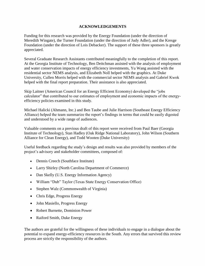
Impact on Power Plant Construction
By 2030, the Reference Scenario forecasts the need for an increase of 49 GW of electricity
capacity in the southern National Electricity Reliability Council (NERC) regions above the
capacity in operation in 2010 (Figure ES.4). This growing demand is expected to be met
primarily by the addition of new combined cycle natural gas plants and new combined natural
gas/diesel plants, along with some additional nuclear power, coal plants, and renewable power
generation. Some oil and natural gas steam plants are retired during this period, as well. This is
represented by the part of the bar in Figure ES.4 that is below the zero axis.
Figure ES.4 Incremental Generating Capacity in 2030
Beyond 2010 -- Southern NERC Regions
In contrast, implementation of vigorous energy-efficiency policies could eliminate the need to
expand overall capacity between 2010 and 2030; in fact, the electricity capacity in the Southern
NERC regions could decrease over the 20-year period by 19 GW. While new plants are needed,
their capacity is more than offset by plant retirements. In addition to retiring more than 20 GW of
oil and natural gas steam plants and some natural gas capacity, the energy-efficiency policies
eliminate the need for all but 7 GW of new capacity, most of which is expected to be nuclear and
natural gas powered, based on the SNUG-NEMS model. Very little new renewable capacity is
added in this Energy-Efficiency scenario because the addition of new capacity of any type is
minimized, and most renewable power options exceed the cost of power production by new
combined cycle natural gas plants.
-40
-20
0
20
40
60
80
Reference with EE Policies
GW
Renewables
Nuclear Power
Comb Turbine/Diesel
Combined Cycle
Oil & NG Steam
Coal
Less 19 GW new capacity net
49 GW new capacity net

xii
Economic Impacts
The public and private investments stimulated by the energy-efficiency policies outlined in this
study could reduce energy bills in the South, moderate electricity rate increases, create new
employment opportunities, and expand the region‟s level of economic activity (i.e., Gross
Regional Product) (Table ES.1).
Table ES.1 Economic and Employment Impacts of
Energy-Efficiency Policies in the South
2020 2030
Annual Energy Savings
(billion $2007) $40.9 $71.0
Annual Public and Private Investment
(billion $2007) $15.8 $22.4
Annual Increased Employment (From
Productive Investment and Energy
Savings) (in full-time-equivalents)
380,000 520,000
Impact on Gross Regional Product
(GRP) (billion $2007)
$1.23 $2.12
Energy Bill Savings. Consumers in the South could save $41 billion in reduced energy bills in
the year 2020 as a result of the portfolio of nine energy-efficiency policies. These energy bill
savings increase to $71 billion in 2030. For example, a typical household in the South would
save $26 on its monthly electricity bill in 2020, and would save $50 each month in 2030. In
addition to directly benefiting the consumers who make energy-efficiency investments, these
policies benefit all consumers because the reduction in overall energy consumption causes
energy prices to rise more moderately than would otherwise occur.
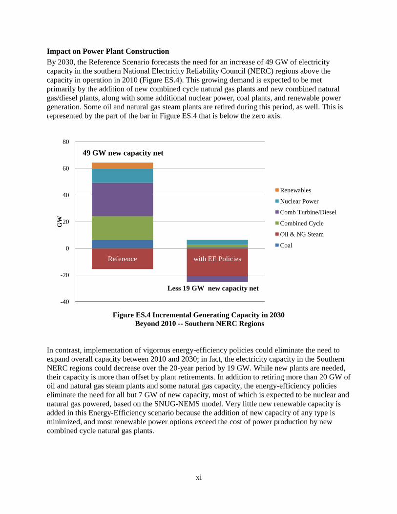
Electricity Rate Impacts. The portfolio of nine energy-efficiency policies modeled together
would lead to a moderation of the energy price escalation that is otherwise forecast to occur over
the next two decades (Table ES.2). For example, residential electricity rates in 2030 would be
17% lower in the Energy-Efficiency scenario than in the Reference Scenario. The reduced prices
resulting from improved energy efficiency occur for both electricity and natural gas and across
all sectors. The moderating impact on electricity rates grows over time as electricity consumption
declines relative to the Reference case.
xiii
Table ES.2 The Effect of Energy-Efficiency Policies on
Expected Southern Electricity Rates
2015 2020 2025 2030
Residential -3% -8% -11% -17%
Commercial -1% -6% -8% -13%
Industrial -3% -8% -11% -16%
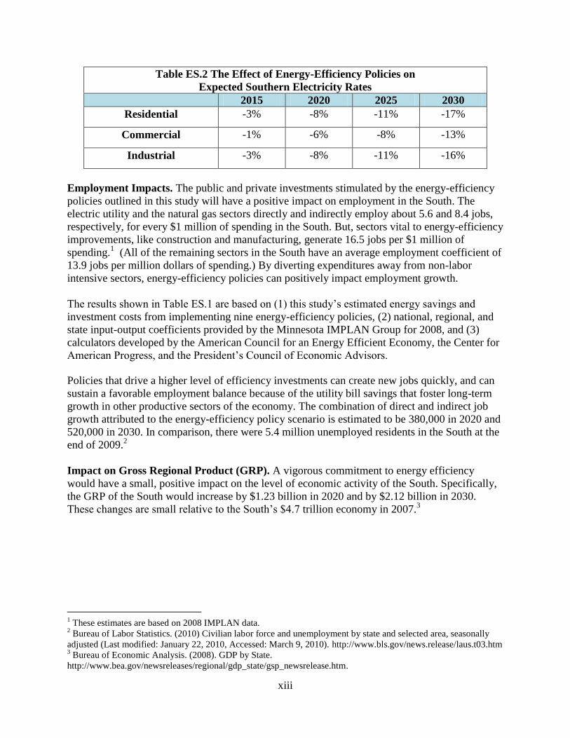
Employment Impacts. The public and private investments stimulated by the energy-efficiency
policies outlined in this study will have a positive impact on employment in the South. The
electric utility and the natural gas sectors directly and indirectly employ about 5.6 and 8.4 jobs,
respectively, for every $1 million of spending in the South. But, sectors vital to energy-efficiency
improvements, like construction and manufacturing, generate 16.5 jobs per $1 million of
spending.1 (All of the remaining sectors in the South have an average employment coefficient of
13.9 jobs per million dollars of spending.) By diverting expenditures away from non-labor
intensive sectors, energy-efficiency policies can positively impact employment growth.
The results shown in Table ES.1 are based on (1) this study‟s estimated energy savings and
investment costs from implementing nine energy-efficiency policies, (2) national, regional, and
state input-output coefficients provided by the Minnesota IMPLAN Group for 2008, and (3)
calculators developed by the American Council for an Energy Efficient Economy, the Center for
American Progress, and the President‟s Council of Economic Advisors.
Policies that drive a higher level of efficiency investments can create new jobs quickly, and can
sustain a favorable employment balance because of the utility bill savings that foster long-term
growth in other productive sectors of the economy. The combination of direct and indirect job
growth attributed to the energy-efficiency policy scenario is estimated to be 380,000 in 2020 and
520,000 in 2030. In comparison, there were 5.4 million unemployed residents in the South at the
end of 2009.2
Impact on Gross Regional Product (GRP). A vigorous commitment to energy efficiency
would have a small, positive impact on the level of economic activity of the South. Specifically,
the GRP of the South would increase by $1.23 billion in 2020 and by $2.12 billion in 2030.
These changes are small relative to the South‟s $4.7 trillion economy in 2007.3
1 These estimates are based on 2008 IMPLAN data.
2 Bureau of Labor Statistics. (2010) Civilian labor force and unemployment by state and selected area, seasonally
adjusted (Last modified: January 22, 2010, Accessed: March 9, 2010). http://www.bls.gov/news.release/laus.t03.htm 3 Bureau of Economic Analysis. (2008). GDP by State.
http://www.bea.gov/newsreleases/regional/gdp_state/gsp_newsrelease.htm.

xiv
Cost-Effectiveness of the Portfolio of Energy-Efficiency Policies
As Table ES.3 shows, the portfolio of nine energy-efficiency policies is cost-effective. The two
policies addressing commercial buildings have the highest combined ratio of benefits to costs
using the “total resource cost test.” Over the 20-year period, an investment of $31.5 billion4
would generate energy bill savings of $126 billion. Energy bill savings would begin immediately
in 2010, would grow through 2030, and would then taper off until 2050 when the useful life of
the improved technologies is expected to end. The result is a benefit/cost (B/C) ratio of 4.0 for
the commercial sector. That is, for every dollar invested by the government and the private
sector, four dollars of benefit is received. The industrial and residential sector policies are
similarly cost effective with B/C ratios of 3.4 and 1.3.
The savings from the greater efficiency stimulated by these nine policies would total
approximately $448 billion in present value to the U.S. economy. It would require an investment
over the 20-year planning horizon of approximately $200 billion in present value terms. These
costs include both public program implementation costs as well as private-sector investments in
improved technologies and practices.
Among the nine individual policies, only two have benefit/cost ratios of less than one –
indicating that they are not cost-effective. These include appliance incentives and standards (with
a B/C ratio of 0.3) and combined heat and power incentives (with a B/C ratio of 0.7). When
clothes washers and refrigerators are removed from the suite of appliance standards with
incentives, the B/C ratio rises to 0.7. When carbon dioxide emission reductions are valued at a
range of $15 per metric ton in 2010 rising to $51 in 2030), both of these policies approach or
exceed the breakeven B/C ratio of 1.
According to the total resource cost test, the most cost-effective policy is tighter commercial
appliance standards (with a B/C ratio of 4.6) followed by B/C ratios of 4.5 for industrial plant
utility upgrades and 4.1 for residential building codes with third-party verification. These high
B/C ratios combined with the fact that we examined an incomplete set of policies and
technologies suggests that greater levels of investment could generate additional, cost-effective
energy savings.
4 In 2007 dollars, using a 7% discount rate.

xv
Table ES.3 Total Resource Cost Tests by Sector (Million $2007)
Residential Sector Policies
NPV Cost NPV Benefit B/C Ratio
Building Codes with
Third-Party
Verification
$10,000
$41,400
4.1
Appliance Incentives
and Standards
$25,500
$7,060
0.3
Expanded
Weatherization
Assistance Program
$5,840
$6,420
1.1
Residential Retrofit
and Equipment
Standards
$86,600
$119,000
1.4
Combined Policies $115,000 $143,000 1.3
Commercial Sector Policies
NPV Cost NPV Benefit B/C Ratio
Tighter Commercial
Appliance Standards
$26,300 $109,000 4.6
Commercial Retrofit
Incentives
$8,540 $20,900 2.4
Combined Policies $31,500 $126,000 4.0
Industrial Sector Policies
NPV Cost NPV Benefit B/C Ratio
Industrial Plant
Utility Upgrades
$10,800
$48,400
4.5
Industrial Process
Improvement Policy
$36,000
$128,811 3.6
Combined Heat and
Power Incentives
$16,900 $11,400
$17,600*
0.67
1.04*
Combined Policies $53,200 $179,000 3.4 * Includes the environmental benefits from CO2 emissions avoided by CHP systems.
Water Conservation from Energy Efficiency
Water conservation is an important co-benefit of policies that promote the efficient use of
electricity. Based on a water calculator developed for this project, the freshwater consumed in
the process of cooling conventional and nuclear thermoelectric power plants in the Southern
NERC regions is forecast to grow to 334 billion gallons in 2020 and 381 billion gallons in 2030.
Implementation of the nine Energy-efficiency policies examined here could avoid generation that
in turn would save southern NERC regions 8.6 billion gallons of freshwater in 2020 and 20.1
billion gallons in 2030. On a percentage basis, this represents 56% of the projected growth in
water consumption over the next decade, and 43% of the projected growth for the following

xvi
decade. These savings in 2030 represent about one-quarter of the current total water needs of the
City of Atlanta.
Policy Supply Curves for Energy Efficiency in the South
Energy-efficiency supply curves have typically focused on individual technologies. Since the
emphasis of this report is on energy-efficiency potential that is achievable with policy initiatives,
we have developed policy supply curves. The magnitude of energy demand resources that can be
achieved by launching aggressive energy-efficiency policies is shown along the horizontal axis,
and the vertical axis presents the levelized cost of delivering these energy demand resources. The
policies are ordered from the lowest to the highest levelized cost. Only the electricity supply
curve is presented here, in Figure ES.5. Chapter 6 also presents energy-efficiency supply curves
for total energy savings and natural gas. In all cases, we focus on the year 2020.
The electricity efficiency supply curve for the South (Figure ES.5) illustrates how more than
2,000 TBtu of electricity savings could be realized from implementing eight energy-efficiency
policies. (The combined heat and power policy could not be assigned a levelized cost value.)
Figure ES.5 Supply Curve for Electricity Efficiency Resources in the South in 2020
(RCI Sectors)
The supply curve also highlights the large, low-cost potential of industrial efficiency
opportunities, which together could save more than 500 TBtu of electricity for a levelized cost
that is significantly lower than the price of electricity for industrial consumers (6.2 cents/kWh).
The next most cost-effective efficiency option is the commercial standards policy, followed by

xvii
building codes, bringing the cumulative savings for these four policies to nearly 900 TBtu. When
the retrofit incentives and equipment standards are added, a large additional savings can be
achieved. The three remaining policies do not save as much electricity and are more costly.
The natural gas supply curve distributes approximately 1,450 TBtu of savings across the eight
efficiency policies. Commercial standards and residential building codes offer particularly low-
cost, but somewhat limited natural gas savings. Industrial plant utility upgrades and process
improvements, on the other hand, offer low-cost and large-scale opportunities for natural gas
savings in the South.
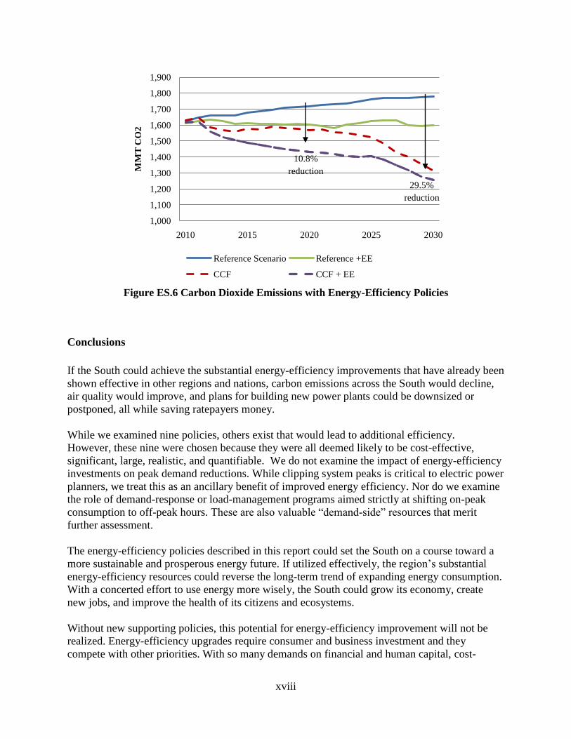
Carbon Constrained Sensitivity Analysis
An analysis of the sensitivity of our study‟s findings to a particular key parameter was
undertaken to ensure the analysis helps capture some of the uncertainties associated with SNUG-
NEMS forecasting. This sensitivity is called the Carbon-Constrained Future (CCF). It was
chosen because the national regulation of greenhouse gases appears possible and will affect how
energy-efficiency policies are perceived and implemented. The scenario is modeled by assuming
a $15/tCO2 price on carbon in 2010, increasing linearly to $51/tCO2 in 2030.
Given our interest in how energy-efficiency policies interact with other supply- and demand-side
initiatives, we evaluated the CCF constraint both on its own and in the presence of energy-
efficiency polices. In this combined set up of CCF + energy-efficiency policies, the effect of
efficiency policies on consumption under the assumption of a Carbon Constrained Future
appears to be additive. That is, the efficiency policies reduce consumption by approximately the
same increment when added to either the Reference scenario or the CCF.
However, this is not to say that there is no interactive effect at all. Rather, the interaction is
apparent when examining the reduction in CO2 emissions. Emission reductions from energy-
efficiency policies result from the consumption of less energy, while the reductions from the
Carbon-Constrained Future result primarily from switching to cleaner fuels. When these two
policy scenarios are imposed simultaneously, the interactions between them grow over time, as
the cleaner fuels predicted in a CCF scenario become the fuels not consumed as the result of
energy-efficiency investments. This effect is noticeable in Figure ES.6 starting around 2025.
xviii
Figure ES.6 Carbon Dioxide Emissions with Energy-Efficiency Policies
Conclusions
If the South could achieve the substantial energy-efficiency improvements that have already been
shown effective in other regions and nations, carbon emissions across the South would decline,
air quality would improve, and plans for building new power plants could be downsized or
postponed, all while saving ratepayers money.
While we examined nine policies, others exist that would lead to additional efficiency.
However, these nine were chosen because they were all deemed likely to be cost-effective,
significant, large, realistic, and quantifiable. We do not examine the impact of energy-efficiency
investments on peak demand reductions. While clipping system peaks is critical to electric power
planners, we treat this as an ancillary benefit of improved energy efficiency. Nor do we examine
the role of demand-response or load-management programs aimed strictly at shifting on-peak
consumption to off-peak hours. These are also valuable “demand-side” resources that merit
further assessment.
The energy-efficiency policies described in this report could set the South on a course toward a
more sustainable and prosperous energy future. If utilized effectively, the region‟s substantial
energy-efficiency resources could reverse the long-term trend of expanding energy consumption.
With a concerted effort to use energy more wisely, the South could grow its economy, create
new jobs, and improve the health of its citizens and ecosystems.
Without new supporting policies, this potential for energy-efficiency improvement will not be
realized. Energy-efficiency upgrades require consumer and business investment and they
compete with other priorities. With so many demands on financial and human capital, cost-
1,000
1,100
1,200
1,300
1,400
1,500
1,600
1,700
1,800
1,900
2010 2015 2020 2025 2030
MM
T C
O2
Reference Scenario Reference +EE
CCF CCF + EE
10.8%
reduction
29.5%
reduction

xix
effective energy-efficiency improvements are easily ignored. Through a combination of
information dissemination and education, financial assistance, regulations, and capacity building,
consumers can be encouraged to invest in energy efficiency. In addition, expanded research and
development and public-private partnerships are needed to innovate and deploy transformational
technologies that enlarge the efficiency potential over the long run.
The ability to convert this vision into reality will depend on the willingness of consumer,
business and government leaders to champion the kinds of policies modeled here.

2
1. INTRODUCTION
For the past several years, U.S. House and Senate committees have debated the pros and cons of
alternative energy and climate legislation. Emerging from this dialogue is a consensus that
energy efficiency should play a key role in transitioning the nation to a clean energy future.
Energy efficiency is generally seen as a large, affordable, and environmentally attractive energy
resource. Investments in energy efficiency can save consumers and businesses money while
reducing pollution, mitigating greenhouse gas (GHG) emissions, and conserving water.
In the electricity sector, evidence has shown that energy efficiency can be as reliable as the
construction of new power plants and the purchase of electricity via long-term contracts or spot
markets (Vine, Kushler, and York, 2007). Energy efficiency is also a low-cost contributor to
system adequacy – the ability of the electric system to supply the aggregate energy demand at all
times. In addition to environmental benefits, energy efficiency often comes hand-in-hand with
productivity gains and job growth.
At the same time, energy efficiency typically requires increased utility and government
incentives, regulations, information, and other policies to overcome barriers and transform
markets. As a result, specific estimates of the size of energy-efficiency resources are highly
variable. The supply of cost-effective energy-efficiency varies according to assumptions made
about future policies, future energy prices, rates of economic growth, and a host of other factors.
Energy Efficiency in the South examines these factors in the design of its detailed primary and in-
depth research on the size of cost-effective energy-efficiency potential in the South.
1.1 GOALS AND ORGANIZATION OF THE REPORT
By implementing new policy approaches that tackle key barriers, create new incentives, set
minimum standards, and enable change, how much energy efficiency can be stimulated? Which
technologies hold the greatest potential and what policies and programs can most effectively
translate that potential into reality? These are the essential questions addressed by this study.
Energy Efficiency in the South is organized into six chapters followed by references and
numerous appendices. The chapters can be grouped into three sections:
Introduction (Chapter 1) and Methodology (Chapter 2): The remainder of this chapter sets the
context for the empirical analysis, describing energy production and consumption in the South
and characterizing current efforts to tap demand-side energy resources. Chapter 2 provides a
broad overview of the methodology used in the policy analysis and energy-efficiency resource
assessments. This chapter also outlines the portfolio of policies modeled in the analysis and
describes the alternative future scenarios that could shape their influence.
Energy-Efficiency Resources, by Sector (Chapters 3-5): These chapters estimate the potential for
cost-effective efficiency policies in each of the Region‟s major sectors: residential and
commercial buildings and industry (the RCI sectors). These assessments begin with a description

3
of energy consumption in the South and the energy-efficiency levels assumed in the “Reference
Scenario” forecast. The chapters then describe each of the energy efficiency policies, the
methodology used to analyze them, and the estimates of energy savings and costs. The chapters
then estimate the cost-effectiveness of each policy, compare their results with other studies, and
describe the limitations including needs for further research.
Integrated Analysis (Chapter 6): This chapter describes the integrated engineering and economic
results of our assessment of energy-efficiency potential in the South. In addition to presenting the
economy-wide cost-effectiveness tests, this chapter characterizes the employment and
macroeconomic impacts of each scenario, as well as the water conservation benefits of the
energy-efficiency policies. In addition to the Reference Scenario forecast, we examine a Carbon
Constrained Future Scenario for a measure of sensitivity analysis. The chapter concludes with a
discussion of the study‟s principal findings.
These chapters are supplemented by detailed appendices that provide additional background on
the current federal policy environment that operates as a backdrop for the proposed new and
expanded policy initiatives, description of our assumptions and methodologies, and in a few
cases, a more detailed description of our findings.
Appendix A describes the hundreds of federal policies and measures that are currently in
place, which seek to promote investments in energy-efficient buildings and industry.
Appendix B provides supplemental information about the study‟s overall methodological
approach.
Appendices C through E provide additional information about the methodologies used to
analyze each sector.
Appendix F provides further information on the baseline analysis and the use of the use
of the ACEEE employment calculator, as well as the methodology used to evaluate water
conservation benefits of the Energy-Efficiency Policy Scenario.
Appendix G contains short (8- to 10-page) profiles of the findings for each of the 16
states in the South, along with the District of Columbia. These profiles are posted on the
website of the Southeast Energy Efficiency Alliance (http://www.seealliance.org/).

4
1.2 OVERVIEW OF THE SOUTH CENSUS REGION
The South census region is comprised of the District of Columbia and 16 States, covering two of
the most populous states in the country – Texas and Florida. The U.S. Census Bureau divides the
South into three divisions. The South Atlantic includes eight states and the District of
Columbia; all but West Virginia sit along the eastern seaboard. The East South Central region
includes Alabama and three states with western borders that touch the Mississippi River. The
West South Central region also includes four states, which all lie west of the Mississippi River.
The South as defined by the U.S. Census Bureau is almost identical to the Region served by the
Southern Governors‟ Association (SGA).5 It is slightly larger than the 11-state region served by
the Southeast Energy Efficiency Alliance.6
Figure 1.1 The South Census Region with Three Divisions7
5All of the SGA member states except for Missouri are located in the South; Missouri is in the West North Central
region. In the South Atlantic region, all states except for DC and DE are member states of SGA. SGA also includes
the U.S. Virgin Islands and Puerto Rico. 6 The region as defined by SEEA includes the 11 states from Kentucky and Virginia south, and from Arkansas and
Louisiana east – see www.seea.us. 7 Map and definition from U.S. Census Bureau document on Regions and Divisions of the United States
www.census.gov/geo/www/us_regdiv.pdf
5
With 36.4% of the country‟s population in 2009, the South is the most populous of the four
census regions of the United States (U.S. Bureau of the Census, 2009). The South region leads
the nation not only in population but also in in-migration and population growth.8 As the nation‟s
largest and fastest growing region, the South has experienced a 20% population growth over the
past decade, and this rapid expansion is expected to continue.
1.3 ENERGY SUPPLY IN THE SOUTH
The South produces significant portions of the nation‟s fossil fuels. In 2007, the region supplied
48% of the nation‟s energy resources, proportionately more for fossil energy resources than for
renewable energy resources. Specifically, the region accounts for the following percentages of
the nation‟s energy production, by fuel (EIA, 2009b):
56% of conventional oil
65% of natural gas marketed production
38% of coal production
43% of nuclear power
28% of renewable energy production.
With a fuel mix for generating electricity that is 77% derived from nonrenewable fossil fuels
(EIA, 2009c), achieving the substantial energy efficiency improvements experienced in many
other parts of the United States would postpone the need for new power plants to meet growing
demand and could improve air quality and reduce carbon emissions across the region. In 12 of
the 16 states in the South, coal is the primary source of power production.
In part because of its heavy reliance on coal and petroleum and it small production (and
consumption) of renewable energy, the South accounts for 41% of U.S. carbon emissions.
1.4 ENERGY USE IN THE SOUTH
The South accounted for 43.6% of the nation‟s total energy consumption in 2006, considerably
more than its share of the country‟s population of 36%. Its higher-than-average per capita energy
consumption is true for each of the major end-use sectors: residential buildings (39%),
commercial buildings (38%), industry (51%), and transportation (41%), and for electric power
(43%).
8 The South has the highest in-migration and population growth in persons, but the West leads the nation in growth
rate on a percentage basis. For the period from 2000 to 2008, population growth for the whole U.S. was estimated at
7.8% with growth for the South at 11.1% and the West at 11.7%; over the same time, the average annual population
growth rate for the whole U.S. was 0.94% with average annual population growth rates for the South at 1.32% and
West at 1.39% (U.S. Bureau of the Census, 2008).

6
1.4.1 Energy Consumption by Source
As is the case nationwide, coal is forecast to increase its share of energy use in the Region
between 2015 and 2030, in the absence of restrictions on CO2 emissions (Figure 1.2). However,
the market share of western coal is expected to increase, while Appalachian coal production is
forecast by EIA to decline slightly. EIA states, “Although producers in Central Appalachia are
well situated to supply coal to new generating capacity in the Southeast, that portion of the
Appalachian basin has been mined extensively, and production costs have been increasing more
rapidly than in other Regions” (EIA, 2008a, p. 84). With 67% of the nation‟s jobs in the U.S.
coal industry supporting only 35% of U.S. coal production, Appalachia has significantly lower
levels of labor productivity and therefore higher costs. In contrast, the Powder River Basin has
vast remaining surface-minable reserves that can be reached by large earth-moving equipment
with significant benefits from economies of scale.
Figure 1.2 Energy Consumption Projection for the South, by Source, 2007-2030
(including transportation, EIA, 2009c)
Availability of reasonably priced and reliable energy has been a value to business in the South
and has helped to drive the region‟s economic development. For example, in 2007, the South
enjoyed an average population-weighted residential electricity price of 10.1 cents per kWh,
compared with a national average of 10.6 cents (EIA, 2009d). Within the South, electricity rates
are lowest in the East South Central Division and highest in the West South Central Division,
although there is variation between and within states accounting for different service providers.
Despite its generous endowment of energy resources, the region is economically challenged. It
accounts for only 33% of the nation‟s gross domestic product (BEA, 2009), and it has the largest
proportion of households living in poverty, of all the Census regions.
As Table 1.1 shows, coal dominates electricity generation in the South, accounting for 54% in
2008, which is slightly higher than the U.S. average of 51%. In contrast, hydropower in the
South, at 2% of generation, is considerably smaller than the 8% national average. The South
0
5
10
15
20
25
30
35
40
45
50
2010 2015 2020 2025 2030
Quad
rill
ion B
tu
Liquid Fuels
Biofuels and Renewables
Nuclear Power
Natural Gas
Coal

7
depends less on renewable sources of electricity than any other region. As a result of this heavy
reliance on fossil fuels, the South accounts for 41% of U.S. carbon emissions. These regional
averages mask a great deal of state-by-state diversity. Three states in the South rely primarily on
natural gas for power production, and one state (South Carolina) relies primarily on nuclear
power.
Table 1.1 Energy Consumption for Electric Power in the South and the U.S.
Coal Renewables Fuel Oil Petroleum
Coke Natural
Gas Nuclear Imports
U.S. 51.3% 8.7% 1.2% 0.4% 17.3% 20.9% 0.3%
South 53.8% 2.9% 1.2% 0.7% 20.8% 20.5% 0.0%
http://www.eia.doe.gov/emeu/states/sep_sum/html/pdf/sum_btu_eu.pdf
EIA forecasts that fuel consumption in the future will correspond to the total energy consumption
projections. EIA forecasts that the South will increase its share of coal consumption for
electricity generation between 2020 and 2030 as shown in Figure 1.3.
Figure 1.3 Energy Consumption for Electric Power Generation in the South, 2007-2030
(EIA, 2008a)
States in other regions of the nation are meeting one to two percent of their electricity
consumption each year with energy efficiency at a cost of approximately $0.03 per kilowatt-hour
(kWh) compared with projected costs of $0.05 to $0.07 per kWh of electricity from coal, gas
combined cycle, wind or nuclear plants (Brown and Chandler, 2008; Kushler, York and Witte,
2004). California, New York, Vermont, and other states have shown that energy efficiency can
represent a low-cost, low-risk energy strategy.
California, in part due to aggressive and sustained energy-efficiency measures, has kept per
capita electricity use flat over recent decades (National Academy of Sciences, 2008). This is in
0
5
10
15
20
25
2010 2015 2020 2025 2030
Quad
rill
ion B
tu
Fuel Oil
Renewable
Nuclear Power
Natural Gas
Coal

8
direct contrast to national trends over the last 25 years, where U.S. per capita electricity use as a
whole has risen about 50%. Rufo and Coito (2002) have shown that the potential for further
energy-efficiency improvements in California remains strong. A similar potential for aggressive
and sustained energy-efficiency programs has been demonstrated in Vermont and other states,
where electricity consumption per capita has remained fairly flat while the state‟s economy has
grown significantly. Thus, these states have shown that energy demand growth can be
significantly reduced without compromising economic growth. The challenge is to move these
energy-efficiency “best practices” to the South.
1.4.2 Energy Consumption by Sector
In 2007, the South consumed 16.6 quads of energy in the industrial sector, more than any other
sector in the South and proportionately more than the industrial sector in the United States as a
whole (Figure 1.4). This high industrial energy consumption reflects the strong industrial base of
this region, and the heavy representation of energy-intensive industries in the South.
Consequently, compared with the nation as a whole, the South consumes slightly less of its
energy on buildings and transportation. The industrial share is projected to decline over time but
the industrial energy will still be the largest portion by far in 2030 (Table 1.2).
Figure 1.4 Energy Consumption Shares in the U.S. and the South
by End-Use Sectors, in 2007
0%
5%
10%
15%
20%
25%
30%
35%
40%
Residential Commercial Industrial Transportation
US South

9
Table 1.2 Energy Consumption Forecast for the South (quadrillion Btu)
Year RCI
Total
Residential
Buildings
Commercial
Buildings Industry
2007 31.7 8.3 6.8 16.6
2020 31.6 8.9 7.9 14.9
2030 33.2 9.8 8.9 14.5
(EIA, 2009c Annual Energy Outlook)
The energy consumption of each sector is forecast to increase over the next 25 years. Compared
to 2007, consumption expands in 2030 to 9.8 quads of energy (18%) in the residential sector, and
8.9 quads (31%) in the commercial sector. In contrast, energy consumption in industry declines
by 13% to 14.5 quads in the year 2030.
1.4.3 Energy Prices
Energy in the South is relatively cheap, and EIA forecasts that this comparative advantage will
continue through 2030. Table 1.3 compares U.S. and Southern prices.
Analysis by the Center for Business and Economic Research (2006), the Electric Power Research
institute (EPRI), and others suggests that residential and commercial consumers are fairly
insensitive in the short-run to increases in the price of electricity. If this price insensitivity
applies across all energy sources, which is likely, then strong policy interventions will be needed
to promote energy-efficient purchases and practices. Notwithstanding short-term price
insensitivity, smart policies can accelerate investments in energy efficiency (Brown, et al, 2001;
Geller et al., 2006). It is this perspective that we actively explore in the analysis that follows.
Table 1.3 Average Energy Prices to All Users in the South and
the United States
(in 2006 dollars per million Btu)
Fuel Type United States The South
2007 2020 2030 2007 2020 2030
Distillate Fuel Oil $19.5 $25.9 $27.9 $19.5 $25.6 $27.4
Natural Gas $11 $10.9 $11.9 $8.2 $8.3 $9.7
Electricity $44.2 $38.6 $41.5 $25.0 $26.4 $29.1
(EIA, 2009c)

10
1.4.4 Carbon Footprint
When the greater intensity of energy consumption in the South is compounded by its lower-than-
average use of renewable fuels, the Region‟s carbon footprint expands well beyond the national
average. A recent study by Brown, Southworth and Sarzynski (2009) estimated the per capita
carbon footprint of the nation‟s largest 100 metropolitan areas, measured in terms of the metric
tons of carbon emissions per capita from the consumption of residential electricity, residential
energy and light duty vehicle and freight trucks fuels. Eleven of the 20 metropolitan areas with
the largest carbon footprints are located in the South (Figure 1.5). Thus, from a climate policy
perspective, while the South may be more vulnerable to the costs associated with any national
climate policy, it could perhaps gain the most by capitalizing on opportunities to transform its
energy system, compared with other areas of the country.
Figure 1.5 Carbon Footprints of Metropolitan Areas in the South, 2005 (Map drawn from data published in Brown, Southworth, and Sarzynski, 2009)
1.5 ENERGY-EFFICIENCY PROGRAMS AND PRACTICES IN THE SOUTH
1.5.1 Illustrative Energy-Efficient Technologies and Policies
A large potential for improved efficiency exists in numerous energy-consuming equipment and
practices. For instance, high-quality adjustable-speed electronic motor drives, once exotic and
costly, are now mass-produced in Asia and are widely used because of their protective and soft-

11
start circuits. High-efficiency compact fluorescent lamps sell for a fifth of their 1983 price, now
that a billion are made yearly. Real prices have fallen several fold in 15 years for electronic
lighting ballasts and heat-reflecting window coatings. The economic potential for energy
efficiency continues to grow (Lovins, 2007).
Layers of energy inefficiency exist throughout the U.S. economy. For example, converting coal
at the power plant into useable light given off by incandescent lamps is only two percent efficient
(National Academy of Sciences, 2008). By simply replacing incandescent bulbs with compact
fluorescents, a four-fold improvement in efficiency can be achieved. The payback period can be
quite short – in this case for compact fluorescent light (CFL) bulbs, less than a year or as little as
a month, depending on how may hours each day the CFL is used. However, as with many (but
not all) energy-efficiency improvements, consumers need to purchase a more expensive device
in order to generate the energy savings. How can reluctant consumers be persuaded to pay more
up front to save money in the future when they often do not understand the sometimes complex
economic analysis that goes into such a purchasing decision?
Energy-efficiency policy mechanisms are numerous and are implemented at all levels of
government from the local jurisdiction and state to the regional and national scale. To make
matters more complicated, energy-efficiency measures and incentives can be delivered by a
multiplicity of actors and agents, including independent organizations, non-government
statewide organizations, fully integrated independently owned utilities, unaffiliated distribution
companies, as well as government agencies (Harrington and Murray, 2003). In this report, we
use the typology developed by the Committee on Climate Change Science and Technology
Integration (2009) to inventory existing policies and to consider alternatives (see Appendix A).
Together, energy efficiency and demand response can delay or completely avoid the need for
expensive new generation and transmission investments, thus keeping the future cost of
electricity affordable and freeing up energy dollars to be spent on other resources to expand the
Region‟s economy. A greater share of the dollars invested in energy efficiency goes to local
companies that create new jobs compared with conventional electricity resources where much of
the money flows out of the Region to equipment manufacturers and fuel suppliers.

12
1.5.2 Energy-Efficiency Practices in the South
The Digest of Climate Change and Energy Initiatives in the South (SSEB, 2009) provides an
overview of the climate change and energy policy initiatives currently underway in the South. It
catalogues a large number of energy efficiency programs currently operating throughout the
region. In summarizing the nature of these initiatives, it concludes the following about the
approach of the South:
“Rather than attempting to craft regional cap and trade programs or mandating
specific technologies, Southern states are focusing on incentives for building
energy efficiency, fostering a bioeconomy through industry, supporting research
and development of clean energy technologies and adopting „lead by example‟
policies for state governments.” (SSEB, 2009, p. 5)
Other assessment of energy policies have noted that per capita spending on electric utility energy
efficiency programs in the Southeast is just one-fifth the national average (Elliott et al., 2003;
Elliott and Shipley, 2005). In 2003 and 2005, ten southern states were given a “D” grade for
current policies and environment (the lowest grade given to any state). Texas was the only state
in the South to receive an “A”. For context, of the 48 contiguous states, the grades distributed
were: A (12), B (12), C (8), and D (16).
As illustrated in Table 1.4, States in the South are comparable to the nation as a whole in terms
of their adoption of 2006 (or more recent) International Energy Conservation Codes for
residential and commercial buildings. On the other hand, their adoption of Leadership for
Environment and Energy Design (LEED) standards for State buildings is much lower than the
national average, as is the market penetration of Energy Star Homes.
In terms of utility policies that support energy efficiency investments, southern States also lag
behind the rest of the nation. Only 71% of the States in the South have adopted net metering
policies. Net metering allows customers with small generating facilities to use a single meter to
measure both power drawn from the grid and power fed back into the grid from on-site
generation. This enables customers to receive retail prices for the excess electricity they
generate, which can be critical to the economic viability of industrial combined heat and power
systems as well as on-site renewable generation.
Only a few States in the South have adopted provisions to decouple profits from sales of either
electricity or natural gas, to provide a “level playing field” for energy efficiency. “Decoupling”
of utility revenues and profits can be achieved either through periodic and frequent true-ups of
projected sales or by other mechanisms that provide utilities with timely cost recovery and
earnings opportunities for operating energy-efficiency programs (Brown, et al., 2009). Similarly,
only four southern states have undergone active electric utility restructuring, three are part of
regional carbon cap and trade programs, and only two have promulgated state appliance or
equipment standards that exceed federal requirements.

13
Table 1.4. Energy Efficiency Policies Implemented by States in the South
Census
Division State
IECC 2006 Building Code
or Better
LEED
Standard or
Equivalent
for State
Buildings
Market
Penetration
of Energy
Star Homes
> 20%
Net
Metering
State
Policy Commercial Residential
South
Atlantic Delaware
D.C.
Florida
Georgia
Maryland
North Carolina
South Carolina
Virginia
West Virginia
East
South
Central
Alabama
Kentucky
Mississippi
Tennessee West
South
Central
Arkansas
Louisiana
Oklahoma
Texas
South Total 9/17 9/17 6/17 3/17 12/17
U.S. Total 29/51 27/51 24/51 13/51 44/51

14
Table 1.4. Energy Efficiency Policies Implemented by States in the South (cont.)
Census
Division State
Decoupling Active
Electricity
Restructuring
by State
Regional
Carbon
Cap and
Trade
Appliance
and
Equipment
Standards Natural
Gas Electricity
South
Atlantic Delaware
D.C.
Florida
Georgia
Maryland
North Carolina
South Carolina
Virginia
West Virginia East
South
Central
Alabama
Kentucky
Mississippi
Tennessee West
South
Central
Arkansas
Louisiana
Oklahoma
Texas
South Total 4/17 2/17 4/17 3/17 2/17
U.S. Total 18/51 6/51 15/51 33/51 13/51
Sales data suggest a low market penetration of energy-efficiency products in the South. For
Energy Star appliances with sales data that are tracked by EPA, the South has the lowest rates of
market penetration (McNary, 2009). This purchase behavior is undoubtedly a function of the
historically low electricity rates that the South has enjoyed. It would also appear to reflect a
relatively weak energy conservation ethic. Evidence of this is provided by the results of a poll
conducted in January 2009 by Public Agenda.
The poll suggests that Americans are divided geographically in terms of their views on energy
conservation and regulating energy use and prices versus exploring, mining, drilling and
construction of new power plants. Yuliya Chernova, a reporter in New York for Clean
Technology Insight, a Dow Jones & Co. newsletter, notes that conservation is supported by a

15
large majority nationwide, however, it is close to even with exploration and drilling in the South,
48% to 45%, (Figure 1.6).
Figure 1.6 Public Agenda Poll
(Chernova, 2009)
On the other hand, utilities in the South have embraced demand-side management as a means of
reducing the peak power requirements of their largest customers. According to Goldman (2006),
there were 2,700 commercial and industrial customers enrolled in TOU programs in 2003,
representing 11,000 MW. Three utility programs in the Southeast (TVA, Duke Power, and
Georgia Power) account for 80% of these participants, and they primarily engage large energy
users.
1.5.3 Previous Estimates of Energy-Efficiency Potential in the South
Many studies have examined the potential for deploying greater energy efficiency in the South.
Nineteen of these were recently examined in a “meta-review” by Chandler and Brown (2009).
These studies contain more than 250 estimates of the energy efficiency potential for different
fuels (electricity, natural gas, and other fuels), sectors of the economy (residential buildings,
commercial buildings, and industry), and types of potential (technical, economic, maximum
achievable, and moderate achievable).
The meta-review concludes that a reservoir of cost-effective energy savings exists in the South.
The full deployment of these nearly pollution-free opportunities could largely offset the growth
in energy consumption forecast for the region over the next decade. Such deployment would

16
reduce capacity-related costs associated with the expansion of electricity and natural gas
infrastructure and supply. The full deployment of energy-efficient technologies could bring
energy consumption in 2020 down 9 percent below projected levels, which would bring future
consumption to slightly less than present levels, as shown in Figure 1.7. This would entirely
offset the need to expand electricity generation capacity in the South through the year 2020.
Figure 1.7 Achievable Energy Efficiency Potential in the South:
Results of a “Meta Review” (Chandler and Brown, 2009)
By “full deployment” the report means the maximum achievable energy efficiency potential that
is also cost-effective. The meta-review concludes that the South has the technical potential to
reduce its energy consumption over the next decade by 2 percent per year, but some of this
potential is not cost-effective at current energy prices. The region has the economic potential to
reduce its energy consumption by 1.5 percent per year, but some of this potential is not
achievable with feasible policy interventions. With vigorous policies, it is possible to reduce
energy consumption in the South by 1 percent per year, which would more than eliminate the
projected growth in energy demand in the region. “Maximum achievable potential” refers to the
economic energy savings potential that can be achieved with such public policies.
More recently, McKinsey Global Energy and Markets (2009) published an assessment of
economic potential for energy efficiency improvements in the RCI sectors of the U.S.
Specifically, it focused on the opportunities that are “net-present-value positive” and therefore
should be considered to be economically attractive. Their estimates do not discount economic
potentials to reflect the difficulty of realizing these opportunities through policy or other
interventions.
17
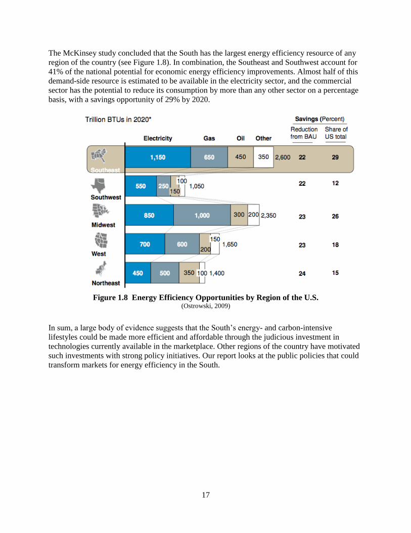
The McKinsey study concluded that the South has the largest energy efficiency resource of any
region of the country (see Figure 1.8). In combination, the Southeast and Southwest account for
41% of the national potential for economic energy efficiency improvements. Almost half of this
demand-side resource is estimated to be available in the electricity sector, and the commercial
sector has the potential to reduce its consumption by more than any other sector on a percentage
basis, with a savings opportunity of 29% by 2020.
Figure 1.8 Energy Efficiency Opportunities by Region of the U.S.
(Ostrowski, 2009)
In sum, a large body of evidence suggests that the South‟s energy- and carbon-intensive
lifestyles could be made more efficient and affordable through the judicious investment in
technologies currently available in the marketplace. Other regions of the country have motivated
such investments with strong policy initiatives. Our report looks at the public policies that could
transform markets for energy efficiency in the South.

18
2. METHODOLOGY
Many different approaches have been used to assess the potential for improved energy efficiency
in the United States. They are often classified as either “bottom-up” or “top-down.”9 We use a
hybrid approach that combines the strengths of both. Specifically, by using a version of the
National Energy Modeling System (a multi-regional general equilibrium model) supplemented
by spreadsheet analysis our approach produces technologically explicit and behaviorally realistic
results typical of a “bottom-up” approach. By evaluating these technology and behavioral effects
including the Global Insight macroeconomic module, we are able to account for the economy-
wide macroeconomic feedback effects, which are the strength of “top-down” approaches.
This chapter provides an overview of the methodology we developed to estimate cost-effective
and achievable energy-efficiency improvements in the South. The general approach and
methodology is summarized in a flow chart showing eight interrelated steps (see Figure 2.1). The
policy-specific methodologies are summarized in each chapter and detailed in Appendices B
through E. We do not examine the transportation sector.
The first step involves identifying a set of policies that could effectively transform markets for
energy efficiency in residential and commercial buildings and industry – the RCI sectors (box
1).10
The Energy Efficiency Policies were then evaluated based on the published literature and
spreadsheet analysis (box 2). Simultaneously, we considered how to model these policies in
SNUG-NEMS11
(box 3). Testing and modeling these policies in SNUG-NEMS was an iterative
process. Often a preliminary policy design was fine-tuned as results were evaluated (box 4). For
example, modeling the extension of tax incentives for industrial CHP systems was found to have
only a minor impact in the absence of expanded R&D to deliver superior technologies over the
20-year period; as a result, the fiscal policy was enhanced with an increased R&D effort.
Eventually when the modeling of individual policies delivered the types of effects consistent
with the literature, SNUG-NEMS (including Global Insight‟s macro-economic module to ensure
system-side adjustments) used to calculate changes in energy consumption and rates, capacity
and generation, as well as utility bills (box 5).
The resulting indicators were then used to perform three different analyses. First, economic
analysis using total resource cost test, for each of the policies (box 6). Second, results were
transformed into state level values so that our key results could be presented at a level of
geographic granularity that exceeds the NEMS outputs. GRP impacts were estimated with the
9 Supply curves of energy savings and carbon mitigation opportunities are an example of a bottom up approach.
They provide a means of identifying least-cost technology investments (McKinsey, 2009); however, they do not
fully account for cross-sector influences and price feedback effects. “Top-down” approaches use macroeconomic
models to identify the response of markets to changes in energy prices. They typically do not offer the degree of
technology specificity needed to understand how markets are responding.
10
These policies are implemented in the same manner for both the Reference Scenario forecast that does not assume
the creation of a price on greenhouse gases, and for a Carbon-Constrained Future scenario forecast that assumes the
promulgation of a generic carbon cap and trade or another carbon constrained system. The specifics of the CCF
scenario are described in Section 2.5.
11
SNUG-NEMS is Southeast NEMS User Group, a version of EIA‟s NEMS, described in Section 2.2.

19
ACEEE calculator tool (box 7). Regional results are provided in the main report, while state
level results can be found in Appendix G. Third, an off-line spreadsheet was developed to
analyze the SNUG-NEMS output on electricity plants in the South to estimate the impact of the
Energy-Efficiency Policy Scenario on water consumption (box 8).
Figure 2.1 Flow Diagram of Study’s Methodology
The advantage of using an integrated energy model for this type of analysis, one that evaluates a
range of policy options both separately and together, is that such a model captures a wide array
of associated costs, benefits, and interactive effects, as well as robust feedback. An integrated
model can capture second order effects, price interactions (unlike spreadsheet models or supply
curves), the impacts of regional actions on individual states, and non-participant economic
effects. In additional, sensitivity analysis requires fewer assumptions, and layering policies one
on top of another is relatively easy.
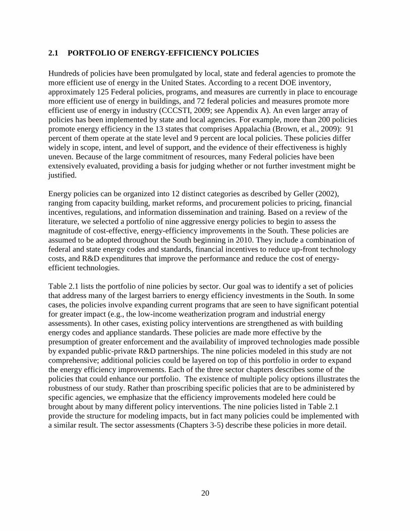
20
2.1 PORTFOLIO OF ENERGY-EFFICIENCY POLICIES
Hundreds of policies have been promulgated by local, state and federal agencies to promote the
more efficient use of energy in the United States. According to a recent DOE inventory,
approximately 125 Federal policies, programs, and measures are currently in place to encourage
more efficient use of energy in buildings, and 72 federal policies and measures promote more
efficient use of energy in industry (CCCSTI, 2009; see Appendix A). An even larger array of
policies has been implemented by state and local agencies. For example, more than 200 policies
promote energy efficiency in the 13 states that comprises Appalachia (Brown, et al., 2009): 91
percent of them operate at the state level and 9 percent are local policies. These policies differ
widely in scope, intent, and level of support, and the evidence of their effectiveness is highly
uneven. Because of the large commitment of resources, many Federal policies have been
extensively evaluated, providing a basis for judging whether or not further investment might be
justified.
Energy policies can be organized into 12 distinct categories as described by Geller (2002),
ranging from capacity building, market reforms, and procurement policies to pricing, financial
incentives, regulations, and information dissemination and training. Based on a review of the
literature, we selected a portfolio of nine aggressive energy policies to begin to assess the
magnitude of cost-effective, energy-efficiency improvements in the South. These policies are
assumed to be adopted throughout the South beginning in 2010. They include a combination of
federal and state energy codes and standards, financial incentives to reduce up-front technology
costs, and R&D expenditures that improve the performance and reduce the cost of energy-
efficient technologies.
Table 2.1 lists the portfolio of nine policies by sector. Our goal was to identify a set of policies
that address many of the largest barriers to energy efficiency investments in the South. In some
cases, the policies involve expanding current programs that are seen to have significant potential
for greater impact (e.g., the low-income weatherization program and industrial energy
assessments). In other cases, existing policy interventions are strengthened as with building
energy codes and appliance standards. These policies are made more effective by the
presumption of greater enforcement and the availability of improved technologies made possible
by expanded public-private R&D partnerships. The nine policies modeled in this study are not
comprehensive; additional policies could be layered on top of this portfolio in order to expand
the energy efficiency improvements. Each of the three sector chapters describes some of the
policies that could enhance our portfolio. The existence of multiple policy options illustrates the
robustness of our study. Rather than proscribing specific policies that are to be administered by
specific agencies, we emphasize that the efficiency improvements modeled here could be
brought about by many different policy interventions. The nine policies listed in Table 2.1
provide the structure for modeling impacts, but in fact many policies could be implemented with
a similar result. The sector assessments (Chapters 3-5) describe these policies in more detail.

21
Table 2.1 Portfolio of Energy-Efficiency Policies
Residential
Buildings
Commercial
Buildings
Industry
Appliance Incentives and
Standards
Aggressive Commercial
Appliance Standards
Process Improvement
Policy
Residential Retrofit and
Equipment Standards
Commercial Retrofit
Incentives
Assessments of Plant
Utility Upgrades
Expanded Weatherization
Assistance Program
Combined Heat and Power
Incentives
Building Codes with
Third-Party Verification
2.2 NATIONAL ENERGY MODELING SYSTEM (NEMS)
NEMS models U.S. energy markets and is the principal modeling tool used by EIA and DOE. It
consists of four supply-side modules, four demand-side modules, two conversion modules, two
exogenous modules, and one integrating module (Figure 2.2). NEMS is one of the most credible
national modeling systems used to forecast the impacts of energy, economic, and environmental
policies on the supply and demand of energy sources and end-use sectors. Its “reference case”
forecasts are based on federal, state, and local laws and regulations in affect at the time of the
prediction. The baseline projections developed by NEMS are published annually in the Annual
Energy Outlook, which is regarded as a reliable reference in the field of energy and climate
policy. It is also widely utilized to conduct the sensitivity analyses of alternative energy policies
and to validate research findings conducted by other government agencies including the
Environmental Protection Agency, Lawrence Berkeley National Laboratory, Oak Ridge National
Laboratory, and the Pacific Northwest National Laboratory.

22
Figure 2.2 National Energy Modeling System (NEMS) (EIA, 2008)
The version of NEMS used for this modeling is SNUG-NEMS, which is short for Southeast
NEMS Users Group. Duke and Georgia Tech have calibrated SNUG-NEMS to the stimulus
release of NEMS, in March 2009. Any references to “NEMS” in this report indicate generic
attributes of EIA‟s model. The distinction of SNUG-NEMS is that while it uses all the same
initial data as NEMS, SNUG-NEMS incorporates changes specified for this study and does not
run on EIA‟s system.
2.2.1 The Baseline Forecast
The starting point, or baseline, for any analysis that is measuring avoided energy consumption or
avoided expenses in the future, i.e. something that does not happen that otherwise might have, is
critical to the results. Our baseline forecast (henceforth called Reference Scenario) of energy
consumption for the South, its three Census Divisions, the 16 individual states and the District of
Columbia are derived for this study from the updated Annual Energy Outlook 2009 (AEO2009)12
reference projections. This Reference Scenario forecast takes into account the Economic
Stimulus Package 2009 (EIA, 2009a).
EIA‟s Annual Energy Outlook 2009 provides energy consumption for the nation, its four census
regions, and its nine census divisions, including the three that are in the South (South Atlantic,
East South Central, and West South Central). Energy production projections are provided by
12
The AEO 2009 was released three times. The final version, the “updated AEO 2009” is the one that will be
discussed as the basis for the Baseline Scenario throughout this document.

23
NERC region. The difference between NERC regions and census divisions is illustrated in
Figure 2.3. The lines represent census divisions and the colors the NERC regions.
This Reference Scenario portrays the South in 2030, much as it is today. It assumes that over the
next 20 years, the nation remains uncommitted to climate policy, and coal continues to be an
economically competitive energy resource. As such, energy efficiency is expected to carry the
external benefits of reduced greenhouse gas emissions and improved energy security. Many
energy-efficiency investments are more cost-effective than many supply-side options, but
numerous barriers including the policy environment often hinder energy-efficiency investments
(Prindle, 2007; Brown and Chandler, 2008).
Figure 2.3 Overlapping Census and NERC Regions
(Fritze, 2009)
Because the AEO 2009 includes several strong efficiency policies promulgated in the Energy
Independence and Security Act of 2007 (EISA, 2007) and the American Recovery and
Reinvestment Act of 2009 (ARRA, 2009), it includes more “naturally occurring energy-
efficiency improvement” than was forecast in the AEO 2007. In addition, the AEO 2009 uses
higher energy prices and a slower GDP growth rate.
2.3 DEFINITION OF PROGRAM ACHIEVABLE POTENTIAL
When evaluating the potential for any energy alternative to be deployed in future years, several
types of estimates are generally used (Rufo and Coito, 2002; NYSERDA, 2003; Eldridge, Elliott,
Neubauer, 2008). Technical potential refers to the complete penetration of all energy-efficient
applications that are technologically feasible, regardless of economic cost-effectiveness. We do
not quantify this potential because it would involve assessing many other policies and some that

24
are not cost-competitive. Economic potential is defined as that portion of the technical potential
that is judged cost-effective. While this is a useful way to frame the current potential, it includes
investments that will not occur because decision-makers cannot be assumed to make optimal
decisions every time a technology or practice is selected. Program achievable potential is
defined as the amount of cost-effective (economic) potential that would occur in response to
specific policies such as subsidies and information dissemination. It recognizes that the full
economic potential is difficult to achieve, but that effective policies and programs can cause
much of the cost-effective potential to be realized. As such, program achievable potential is the
focus of our analysis. Of course, the program achievable potential identified in this study is not a
maximum program achievable, as time and modeling constraints kept us from evaluating a wider
range of cost-effect policies.
2.3.1 Cost-Effectiveness Tests
A number of economic approaches have been used to measure the cost-effectiveness of energy
efficiency investments. The most common approaches look at different actors and their
perspective of cost-effectiveness: only program participants, only utilities, society as a whole,
and more narrowly regional utility and customers (NAPEE, 2007b).
We focus on the total resource cost (TRC) test to evaluate the cost-effectiveness of each of the
modeled energy policies. Originally developed to evaluate utility demand-side management
programs (OTA, 1993), the TRC test concludes that a policy or program is considered cost-
effective if the net present value of benefits is greater than the net present value of costs. It is a
measure of the total net benefits of a program from the point of view of the utility and its
ratepayers as a whole. In sum, a policy or program is cost-effective if it does not increase the
total costs of meeting the customers‟ service needs. A seven percent discount rate is used with
the total resource cost test (Office of Management and Budget‟s Circular No. A-94 p. 8).
According to NAPEE (2007b) the total resource cost test includes the following potential
benefits: avoided supply costs (production, transmission, and distribution) based on net energy
and load reductions, as well as other benefits that do not affect a utility such as fuel oil savings
and water savings. Energy efficiency costs include program administration costs and net
participant costs.
Numerous types of co-benefits tend to be excluded from TRC tests, such as improved comfort
and safety, reduced operation and maintenance costs, increased worker productivity, higher
resale value associated with energy-efficient building upgrades, greenhouse gas emission
reductions, and improved air quality. These benefits are often difficult to monetize. For example,
no consensus exists today to place a value on avoiding the emission of a ton of carbon dioxide
(Tol, 2005). Numerous co-costs also tend to be excluded because they, too, tend to be difficult to
monetize, such as aesthetic issues (e.g., associated with compact fluorescent bulbs) and increased
maintenance costs due to unfamiliarity with new energy-efficient equipment.
The reason that the TRC test is well matched for SNUG-NEMS is the same reason that another
approach, the participant cost test, is less so. SNUG-NEMS integrates the effects of the policies
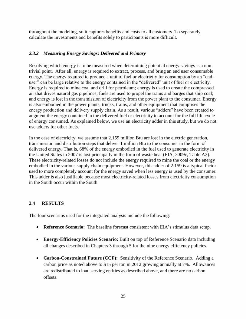
25
throughout the modeling, so it captures benefits and costs to all customers. To separately
calculate the investments and benefits solely to participants is more difficult.
2.3.2 Measuring Energy Savings: Delivered and Primary
Resolving which energy is to be measured when determining potential energy savings is a non-
trivial point. After all, energy is required to extract, process, and bring an end user consumable
energy. The energy required to produce a unit of fuel or electricity for consumption by an “end-
user” can be large relative to the energy contained in the “delivered” unit of fuel or electricity.
Energy is required to mine coal and drill for petroleum; energy is used to create the compressed
air that drives natural gas pipelines; fuels are used to propel the trains and barges that ship coal;
and energy is lost in the transmission of electricity from the power plant to the consumer. Energy
is also embodied in the power plants, trucks, trains, and other equipment that comprises the
energy production and delivery supply chain. As a result, various “adders” have been created to
augment the energy contained in the delivered fuel or electricity to account for the full life cycle
of energy consumed. As explained below, we use an electricity adder in this study, but we do not
use adders for other fuels.
In the case of electricity, we assume that 2.159 million Btu are lost in the electric generation,
transmission and distribution steps that deliver 1 million Btu to the consumer in the form of
delivered energy. That is, 68% of the energy embodied in the fuel used to generate electricity in
the United States in 2007 is lost principally in the form of waste heat (EIA, 2009c, Table A2).
These electricity-related losses do not include the energy required to mine the coal or the energy
embodied in the various supply chain equipment. However, this adder of 2.159 is a typical factor
used to more completely account for the energy saved when less energy is used by the consumer.
This adder is also justifiable because most electricity-related losses from electricity consumption
in the South occur within the South.
2.4 RESULTS
The four scenarios used for the integrated analysis include the following:
Reference Scenario: The baseline forecast consistent with EIA‟s stimulus data setup.
Energy-Efficiency Policies Scenario: Built on top of Reference Scenario data including
all changes described in Chapters 3 through 5 for the nine energy efficiency policies.
Carbon-Constrained Future (CCF): Sensitivity of the Reference Scenario. Adding a
carbon price as noted above to $15 per ton in 2012 growing annually at 7%. Allowances
are redistributed to load serving entities as described above, and there are no carbon
offsets.

26
All Energy-Efficiency Policies and a Carbon Constraint: This sensitivity layers all of
the energy efficiency policies on top of the CCF scenario.
The SNUG-NEMS analysis of the Energy Efficiency Policies looked at the policies from
multiple directions. Policies were evaluated one at a time, together within a sector as well as all
nine policies together. The major results were estimates of reductions in energy consumption by
sector (aka, energy savings), change in electricity and natural gas rates, energy efficiency,
change in electricity generation and new capacity, as well as energy bill changes. Decreased
water demand was evaluated in a spreadsheet, while jobs and gross regional product (macro-
economic indicators) are captured by the DEEPER model.
For the purposes of this study, energy savings is avoided energy consumption in the future due to
program achievable potential from efficiency policies. Energy efficiency refers to the percent
reduction of one future year‟s projected energy consumption represented by the energy savings
in that year, as a result of the program potential. Energy bill savings is a measure of reduced
expenditures associated with energy as a result of efficiency policies and any second order
effects. Changes in future generation and capacity needs due to the policy bundle are reported
by NERC region as NEMS evaluates electricity supply and dispatch as such, while demand is
grouped by census regions (the mapping of census and NERC regions is shown above in Figure
2.3).
As there is no direct mapping of supply and demand regions. Southern totals will have a bit of
uncertainty. Three NERC regions are almost entirely within the Southern census regions, while
two others contain large chunks of Southern states.13
2.5 SENSITIVITY ANALYSIS CASE: CARBON CONSTRAINED FUTURE
The integrated analysis involved combining the residential, commercial, and industrial energy
efficiency policies into one is known as the “Energy-Efficiency Policies” Scenario.
This full policy analysis, is done twice starting at two different points. The Reference Scenario
is the obvious starting point, while the sensitivity case is a future with a carbon constraint (the
“Carbon-Constrained Future” or CCF Scenario). Based on current political concerns it seems
prudent to evaluate whether the Energy Efficiency Policies hold up better, worse or similarly in
the event that a price will be placed on greenhouse gas emissions over the next 20 years.
We approximate the impact of a carbon constraint by adjusting several parameters in SNUG-
NEMS. First, after examining the allowance price projections estimated by the Energy
Information Administration (EIA), Congressional Budget Office (CBO), Environmental
Protection Agency (EPA), and Natural Resource Defense Council (NRDC), we set a carbon
13
Some details of NERC regions mapping to census regions as per Figure 2.3: FERC is part of South Atlantic,
ERCOT is part of WSC region, and SERC other than a piece of Missouri is a piece of all three Southern census
regions. Parts of SPP, including all of Oklahoma overlap with WSC and SA, while ECAR, particularly all of
Kentucky and West Virginia are within ESC and SA respectively. MAAC encompasses the tip of SA.
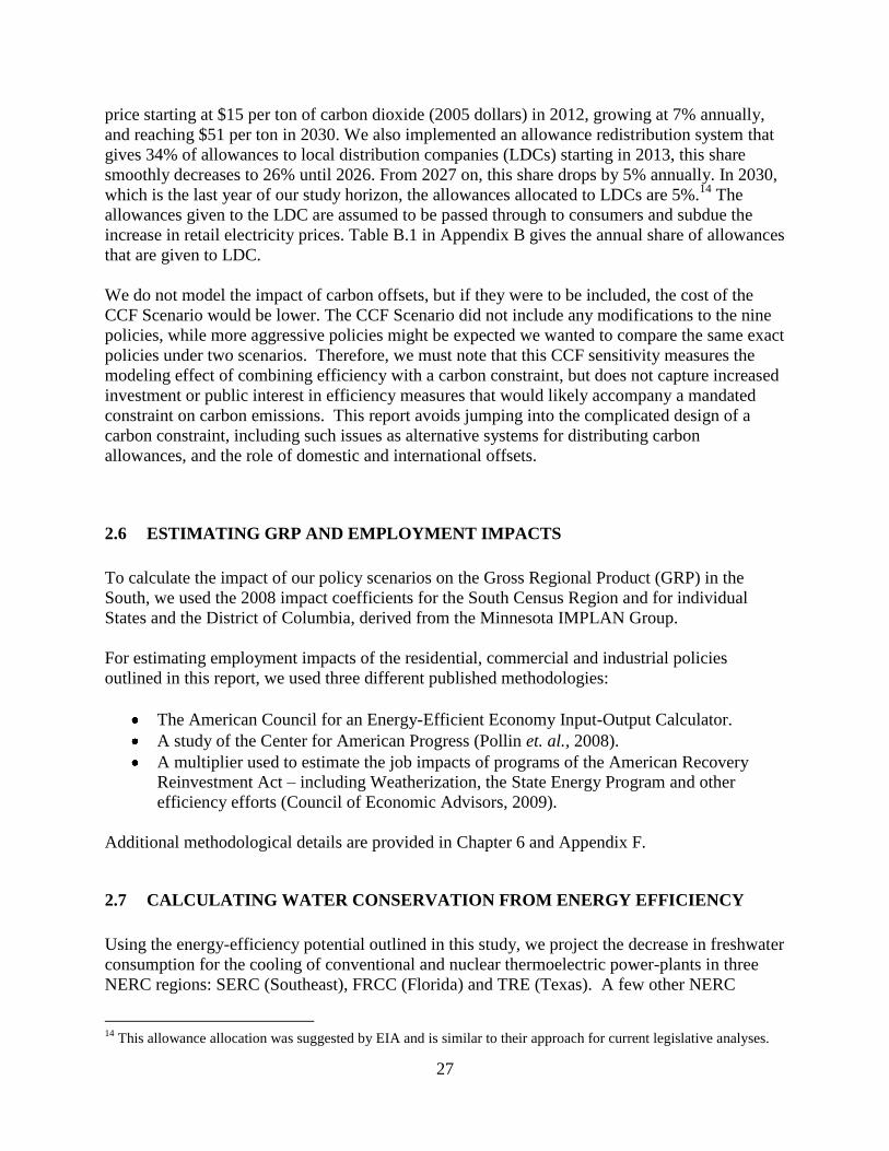
27
price starting at $15 per ton of carbon dioxide (2005 dollars) in 2012, growing at 7% annually,
and reaching $51 per ton in 2030. We also implemented an allowance redistribution system that
gives 34% of allowances to local distribution companies (LDCs) starting in 2013, this share
smoothly decreases to 26% until 2026. From 2027 on, this share drops by 5% annually. In 2030,
which is the last year of our study horizon, the allowances allocated to LDCs are 5%.14
The
allowances given to the LDC are assumed to be passed through to consumers and subdue the
increase in retail electricity prices. Table B.1 in Appendix B gives the annual share of allowances
that are given to LDC.
We do not model the impact of carbon offsets, but if they were to be included, the cost of the
CCF Scenario would be lower. The CCF Scenario did not include any modifications to the nine
policies, while more aggressive policies might be expected we wanted to compare the same exact
policies under two scenarios. Therefore, we must note that this CCF sensitivity measures the
modeling effect of combining efficiency with a carbon constraint, but does not capture increased
investment or public interest in efficiency measures that would likely accompany a mandated
constraint on carbon emissions. This report avoids jumping into the complicated design of a
carbon constraint, including such issues as alternative systems for distributing carbon
allowances, and the role of domestic and international offsets.
2.6 ESTIMATING GRP AND EMPLOYMENT IMPACTS
To calculate the impact of our policy scenarios on the Gross Regional Product (GRP) in the
South, we used the 2008 impact coefficients for the South Census Region and for individual
States and the District of Columbia, derived from the Minnesota IMPLAN Group.
For estimating employment impacts of the residential, commercial and industrial policies
outlined in this report, we used three different published methodologies:
The American Council for an Energy-Efficient Economy Input-Output Calculator.
A study of the Center for American Progress (Pollin et. al., 2008).
A multiplier used to estimate the job impacts of programs of the American Recovery
Reinvestment Act – including Weatherization, the State Energy Program and other
efficiency efforts (Council of Economic Advisors, 2009).
Additional methodological details are provided in Chapter 6 and Appendix F.
2.7 CALCULATING WATER CONSERVATION FROM ENERGY EFFICIENCY
Using the energy-efficiency potential outlined in this study, we project the decrease in freshwater
consumption for the cooling of conventional and nuclear thermoelectric power-plants in three
NERC regions: SERC (Southeast), FRCC (Florida) and TRE (Texas). A few other NERC
14
This allowance allocation was suggested by EIA and is similar to their approach for current legislative analyses.

28
regions include fractions of the South (as shown in Figure 2.3 above), but we chose to focus on
these three which are almost exclusively within the South. Using data from the Electric Power
Research Institute, we estimate average water consumption in gallons per megawatt hour based
on plant and cooling system type (see Chapter 6 and Appendix F for further details).
One assumption made is that half of current plants in use would have once-through cooling
systems, but that all potential new generation would use recirculating (close-loop) systems due to
permitting restrictions on open-loop systems. These assumptions are consistent with NETL and
EIA data. Finally, we assumed that the ratio of freshwater to saltwater from power-plant cooling
would remain consistent in each of the NERC regions (See Table B.2 for USGS data on the
current freshwater and saltwater percentages).
2.8 METHOD FOR DERIVING STATE-SPECIFIC ESTIMATES
For Appendix G, a “proportioning” methodology was used to produce “business as usual”
baseline forecasts for the 16 individual states and the District of Columbia, which comprise the
Census-defined South. The forecasts are derived from the third version of Annual Energy
Outlook 2009 (AEO2009) reference projections, which takes into account the Economic Stimulus
Package 2009 (EIA, 2009a). The methodology is based on the approach used by Stan Hadley in
his study of the energy efficiency and renewable energy potential in North Carolina (Hadley,
2003).
EIA‟s Annual Energy Outlook 2009 provides energy consumption and production projections for
the nation, its four census regions, and its nine census divisions, including the three that are in
the South (West South Central, and East South Central, and South Atlantic). To create state
estimates, we combine the values for all states in each census division and calculate the share of
each state to the total. In addition to the method, we adjust the state specific proportions,
considering the variation and difference in population growth rates across the states.
The Southern Energy Efficiency Center (SEEC) has developed measurement and verification
protocols to estimate the energy consumption of individual states. According to that study, the
energy use per capita of each southern state in each sector has been relatively constant over the
last decade. The SEEC study supports our assumption that the energy use by state increases
proportionally to the population growth.
The methodology used here involves four steps:
• First, we calculated the Normalized Energy Use per Capita (NEUC) from 2004 to 2006
with the historical energy consumption and population by state from the EIA‟s State
Energy Data System (SEDS) (EIA, 2009e).
• Second, we approximated the energy use by state with the fixed NEUC and population
projections from the U.S. Census Bureau.
• Then, we derived the annual share of each state to the total division.
• Finally, using the state specific percentages, we allocated out the regional AEO
projections to each state.

29
3. ENERGY EFFICIENCY IN RESIDENTIAL BUILDINGS
3.1 INTRODUCTION TO THE RESIDENTIAL BUILDINGS IN THE SOUTH
In 2007, the total residential consumption in the South Census Region was 8.52 quadrillion Btu.
This represented 19.5% of the total energy consumption in the region. Nationally, the residential
sector was 21.3% of total energy consumption. Due to the South‟s heavy industrial energy
consumption, the residential sector represents less of the total South‟s energy consumption than
that of the nation (EIA, 2009a; Table S1). Though the residential sector is a smaller fraction of
the total energy consumed, per capita residential energy consumption is higher than the national
average. In 2007, the South had an estimated 36.6% of the nation‟s population while its
residential sector consumption was 39.5% of all U.S. residential consumption (EIA, 2009a;
Census, 2009a). This higher energy consumption points to a greater potential for residential
energy efficiency in the South than the rest of the nation.
The South‟s residential sector relies more on electricity than the national average. Retail
electricity sales composed 27% of residential consumption in the South compared to 22%
nationally (EIA, 2009b; Table S4). Since electricity generation in the South is more reliant on
coal, natural gas, and petroleum than the nation (EIA, 2009c; Table S8), the electricity consumed
in the South is more carbon intensive and is associated with higher electrical system losses.
Figure 3.1 compares residential fuel consumption between the South and the United States.
Figure 3.1 Residential Sector Consumption in the South and US, 2007 (EIA, 2009b)
The historical and projected energy consumption by the South‟s residential sector is shown in
Figure 3.2. Historical consumption is shown from 1960 to 2007 (EIA, 2009d). The projected
consumption is shown from 2007 to 2030 and is expected to increase 18% from 2010 to 2030
(EIA, 2009).
Liquid Fuels
Subtotal
2.6%
Natural Gas
11%
Coal
.01%
Renewables
2%
Electricity
27%Electricity
Related
Losses58%
South
Liquid
Fuels
Subtotal5.8%
Natural Gas
22%
Coal
.03%
Renewables
3%
Electricity
22%
Electricity
Related
Losses47%
United States
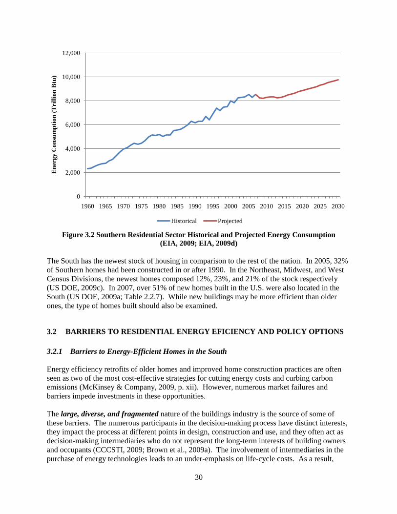
30
Figure 3.2 Southern Residential Sector Historical and Projected Energy Consumption
(EIA, 2009; EIA, 2009d)
The South has the newest stock of housing in comparison to the rest of the nation. In 2005, 32%
of Southern homes had been constructed in or after 1990. In the Northeast, Midwest, and West
Census Divisions, the newest homes composed 12%, 23%, and 21% of the stock respectively
(US DOE, 2009c). In 2007, over 51% of new homes built in the U.S. were also located in the
South (US DOE, 2009a; Table 2.2.7). While new buildings may be more efficient than older
ones, the type of homes built should also be examined.
3.2 BARRIERS TO RESIDENTIAL ENERGY EFICIENCY AND POLICY OPTIONS
3.2.1 Barriers to Energy-Efficient Homes in the South
Energy efficiency retrofits of older homes and improved home construction practices are often
seen as two of the most cost-effective strategies for cutting energy costs and curbing carbon
emissions (McKinsey & Company, 2009, p. xii). However, numerous market failures and
barriers impede investments in these opportunities.
The large, diverse, and fragmented nature of the buildings industry is the source of some of
these barriers. The numerous participants in the decision-making process have distinct interests,
they impact the process at different points in design, construction and use, and they often act as
decision-making intermediaries who do not represent the long-term interests of building owners
and occupants (CCCSTI, 2009; Brown et al., 2009a). The involvement of intermediaries in the
purchase of energy technologies leads to an under-emphasis on life-cycle costs. As a result,
0
2,000
4,000
6,000
8,000
10,000
12,000
1960 1965 1970 1975 1980 1985 1990 1995 2000 2005 2010 2015 2020 2025 2030
En
erg
y C
on
sum
pti
on
(T
rill
ion
Btu
)
Historical Projected

31
homeowners cannot see beyond the relatively high initial costs of energy-efficient appliances
and building construction practices. Similarly, many builders adopt green building practices
because they do not know if higher up-front expenditures will translate into increased sale
values.
Information barriers occur when decision-makers do not possess enough usable information to
make investments that are in their own best interest. Consumers have been found to be largely
unaware of the relationships between their lifestyles, energy consumption, and the environment
(Garrett and Koontz, 2008). Behavioral-related studies have shown that individuals do not know
how much energy appliances or their homes use, do not know where energy comes from, assume
new appliances are efficient, do not consider energy when they make purchasing decisions, and
focus on up-front costs (Lutzenhiser, 2009; DEFRA, 2007; McKeown, 2007). Sometimes
information barriers are compounded by a lack of trusted, actionable information. While a
bounty of facts and data is available to consumers, the information is often presented in terms
that are not specific enough to the consumer to be useful or to drive change.
Outdated building codes and appliance standards represent regulatory barriers to energy-
efficient residential buildings. For example, seven states in the South either do not have
statewide residential building codes, or have outdated codes from 2003 or earlier. Building
standards can also be distortionary, in spite of their numerous positive influences. Because codes
and standards take a long time to adopt and modify, the best performing materials and
technologies are not readily deployed, thereby inhibiting innovation and encouraging obsolete
technology (Brown, et al., 2009a).
Even when states surpass older building codes, their code compliance is often limited. The
continuous updating of existing codes, adoption of new codes, and expansion of code programs
to improve compliance and achieve real energy and financial savings appear to be difficult for
many states because they lack consistent code enforcement and support programs (Yang, 2005;
Zing Communications, 2007, p.23). Building code compliance is difficult to determine,
especially given performance-based standards, where information is not readily available and
determination of measures require unavailable resources that many times may be prohibitively
expensive (Smith and McCullough, 2001; Yang, 2005).
3.2.2 Policy Options
To address these barriers and to support energy efficiency in the residential sector, this study
models four policy packages: residential building energy codes with third party verification,
expansion of the Weatherization Assistance Program, incentives for existing home retrofits with
equipment standards, and improved appliance standards and incentives.
High initial costs, regulatory barriers, and code compliance are addressed by the modeled
policies. Incentives for retrofit equipment and appliances lower the relatively high initial costs
of energy efficient equipment and appliances. The residential building energy codes remove
regulatory barriers by implementing more efficient and updated codes, while third party
verification also improves building code compliance. All standards and regulations also assist in

32
overcoming the building industry‟s fragmented structure and the information shortfalls that
impede voluntary consumer adoption.
The four policy packages are only some of many policy alternatives that may improve residential
energy efficiency and address barriers. Table 3.1 lists examples of policy actions including those
that are modeled, which are presented in italics. Some of the presented policies could be used as
substitutes to the modeled packages, or as complementary actions.
Table 3.1 Policy Actions that Support Residential Energy Efficiency
Actions
Retrofit Incentives
and Equipment
Standards
Residential
Building Codes
with Third-Party
Verification
Appliances
Incentives and
Standards
Expanded
Weatherization
Assistance Program
Research,
Development, and
Demonstration
Development of new
insulation, heating,
and cooling
technologies for local
climates
Support for R&D in
advanced building
processes and
materials
Support for research
and development for
innovation in
appliance
performance
Development of new
insulation, heating,
and cooling
technologies for local
climates
Financing
Low or No-Interest
Loans for Incremental
Cost of Improvements
for Existing Buildings
Low or no-interest
loans for incremental
costs of new
construction
improvements
Support for Energy-
Efficiency Mortgages
(EEMs)
Low or No-Interest
Loans for ENERGY
STAR® Appliances
N/A
Financial Incentives
Retrofits rebates
Tax credits for
efficient purchases
Incremental cost
rebates to builders for
homes that meet or
exceed building
energy code
Permit fee or property
tax reductions for
efficient homes
Efficient appliance
rebates
Tax credits for
efficient purchases
Appliance Buyback
Programs
Grants or publicly
funded provision of
retrofits
Pricing N/A N/A N/A N/A
Voluntary Agreements N/A
Agreement between
major builders in the
area to meet or exceed
code
N/A N/A
Regulations
Allowing third party
compliance inspection
Resale energy rating
and labeling
National efficiency
standards for retrofit
equipment
Model Building
Energy Code
legislation
Allowing third party
compliance inspection
Energy-efficiency
rating and labeling
Broad appliance
standards with tighter
requirements
Standby Efficiency
Standards
National efficiency
standards for
appliances
National standards on
minimum efficiency
for retrofit equipment
and appliances

33
Table 3.1 Policy Actions that Support Residential Energy Efficiency
Actions
Retrofit Incentives
and Equipment
Standards
Residential
Building Codes
with Third-Party
Verification
Appliances
Incentives and
Standards
Expanded
Weatherization
Assistance Program
Information
Dissemination &
Training
Training architects and
contractors
Public Awareness
campaigns to inform
consumers of the
benefits of
conservation and
efficiency measures
Advanced metering
(interior, real-time,
with price signal)
Training architects,
builders, contractors,
and code enforcement
officials
Public Awareness
campaigns to inform
consumers of the
benefits of
conservation and
efficiency measures
Advanced metering
(interior, real-time,
with price signal)
Training contractors,
weatherization
officials, and
community providers
Public Awareness
campaigns to inform
consumers of the
benefits of
conservation and
efficiency measures
Procurement N/A N/A
Government efficient
appliance lead by
example programs
N/A
Market Reforms Enable On-bill
Financing for Retrofits N/A N/A N/A
Planning Techniques N/A
Evaluation and
monitoring for
feedback
N/A N/A
Capacity Building
Centers for energy
efficiency to train next
generation of
architects, builders,
retrofitters
Centers for energy
efficiency to train next
generation of
architects, builders,
retrofitters
Centers for energy
efficiency to train
next generation of
architects, builders,
retrofitters
Centers for energy
efficiency to train next
generation of
architects, builders,
retrofitters
Lighting efficiency policies were not included in this report. Such policies are typically
considered appliance efficiency standards, but the SNUG-NEMS logic handles it separately.
Most of the savings possible through energy-efficient lighting have already been accounted for in
the American Recovery and Reinvestment Act (ARRA) and in the SNUG-NEMS Reference
Scenario (Personal Correspondence with John Cymbalsky, October 1, 2009). The Energy
Independence and Security Act of 2007 (EISA) called for an increase in incandescent bulb
performance and required the Secretary of Energy to consider implementing a minimum standard
of 45 lumens per watt for general service lamps by 2014 (EISA 2007). This effectively phases
out incandescent bulbs, which only produce about 15 lumens per watt. The implementation of
the ARRA in NEMS was done by phasing out inefficient incandescent bulbs starting in 2012,
thereby leading to increased adoption of compact fluorescent light bulbs (CFLs) and light
emitting diodes (LEDs) for this bulb type (Personal Correspondence with John Cymbalsky,
October 1, 2009). In addition to this measure, the American Clean Energy and Security Act
(ACESA) calls for the creation of lighting efficiency standards for outdoor light sockets in 2012
(ACESA, 2009).
The Department of Energy (DOE) has announced new lighting standards that address fluorescent
tubes and recessed can lighting fixtures, which contain reflector lamps (Mufson, 2009). The
more efficient T8 lamps will replace T12 lamps in fluorescent lamps, while both incandescent
and halogen bulbs in reflector lamps will be replaced by highly efficient halogen infrared

34
reflector bulbs (ACEEE, 2009). While the performance standards for general service
incandescent lamps required by the 2007 Energy Independence and Security Act (EISA) are
already accounted for in the 2009 baseline, the new standards will be implemented by the EIA in
the 2010 Annual Energy Outlook (AEO) (Personal communication with John Cymbalsky,
October 1, 2009). Therefore, the savings from the new lighting standards for the year 2010 are
an example of many small savings opportunities that were not captured in our report.
Lastly, if solid-state lighting (SSL) is successfully commercialized such that it achieves its price
and performance levels for full-spectrum white LEDs, it could displace general illumination by
2027 while saving about 1.2 quads in that year alone, which is equivalent to the annual output of
44 large power plants (EERE 2007). This is also one of the opportunities for energy savings that
has not been taken into account in this report.
3.3 ENERGY EFFICIENCY POLICIES IN RESIDENTIAL BUILDINGS
3.3.1 Residential Building Codes with Third-Party Verification
Most states adopted residential energy codes in the 1970s but implementation and enforcement
are not consistent across or between states, which is in part due to the fact that energy codes rank
below health and safety codes as a priority for enforcement (Yang, 2005). As a consequence, the
energy and cost savings potential from building code implementation is not fully achieved.
Figure 3.3 shows a commercially available home with an airtight high-R exterior insulation
finish system (EIFS) that is resistant to moisture and saves more energy than brick, concrete,
stucco, or fiber cement siding (Lapsa, 2009).
Figure 3.3 Exterior Insulation Finish System (Lapsa, 2009)
DOE evaluates states that have the International Energy Conservation Code (IECC) and the
ASHRAE Standard or an equivalent code for residential buildings (US DOE, 2009e). No state in
the South has adopted the IECC 2009 code, its equivalent or better. Florida, the District of
Columbia, Georgia, Kentucky, Louisiana, Maryland, North Carolina, South Carolina, and
Virginia have adopted the IECC 2006 code or better. Arkansas, Tennessee and West Virginia
have adopted the IECC 2003 code, while Texas has adopted the IECC 2001-1998 code.
Meanwhile, Mississippi, Alabama and Oklahoma have adopted no statewide code (US DOE,
2009e). Figure 3.4 presents a map of residential building code adoption in the South.

35
Figure 3.4 Residential Building Codes in the South as of December 2009
Policy Description and Modeling. The policy for reducing energy consumption through more
stringent building codes was modeled by providing a 30% subsidy in the installation costs for
appliances that were covered by the most stringent building codes in NEMS namely. The most
stringent building codes are subsidized by 30% of installation costs for building equipment.
Updated and improved building codes were assumed to be implemented every six years by
eliminating the least stringent code and allowing only the more stringent ones to remain. See
Appendix C-2.1 for further details.
Technology Demand Shifts. As shown in Table 3.2, more aggressive building codes with
increased enforcement can cause a shift in the types of cooling, heating, and water heating
equipment that are bought. The building code policy results in the virtual elimination of new
purchases of room air conditioners and a sizeable increase in the purchase of electric heat pumps
with their inherently high efficiencies. Similarly, electric radiators see a significant decline in
purchase with the building code policy, with electric heat pumps accounting for nearly half of
heating equipment purchased in 2030. For water heating, the building code policy causes a shift
away from natural gas units and toward electric water heating.
Interestingly, the residential code upgrades do not create a large demand for geothermal heat
pumps or solar water heating. Other types of policies (or revised building codes) are needed to
encourage a shift to these renewable alternatives.

36
Table 3.2 Technology Demand Shifts from Building Codes
with Third Party Verification Policy*
Efficiency Reference Policy
End Use Equipment Class 2020 2030 2020 2030 2020 2030
Cooling Central A/C - SEER 14-23 15-23 52% 50% 53% 57%
Electric heat pumps - SEER 13-20 13-21 18% 22% 43% 41%
Geothermal heat pumps - EER 19-30 19-31 0% 0% 2% 2%
Room A/C - EER 11-13 11-13 31% 28% 1% 1%
Heating Electric heat pumps - HSPF 8-11 8-11 27% 33% 44% 49%
Electric radiators --- ---- 33% 29% 20% 7%
Geothermal heat pumps - COP 3.9-5.1 3.9-5.1 0% 1% 2% 2%
LPG furnaces - AFUE 81-96% 82-96% 5% 5% 5% 6%
Natural gas furnaces - AFUE 81-96% 82-96% 27% 26% 27% 35%
Natural gas radiator ---- ---- 4% 4% 1% 1%
Water
heating Electric water heating - EF 0.92-0.95 0.92-0.95 58% 58% 70% 71%
LPG water heating - EF 0.63-1.4 0.86-1.4 2% 2% 4% 4%
Natural gas water heating - EF 0.80-0.85 0.80-0.86 40% 39% 26% 26%
Solar water heating - EF 0.8-4.8 0.8-4.8 0% 0% 0% 0% *These refer to the percentage of new appliances purchased in the reference case and in the policy scenario
in each year.
*SEER = Seasonal Energy Efficiency Ratio
*EER = Energy Efficiency Ratio
*HSPF = Heating Seasonal Performance Factor
*COP = Coefficient of Performance
*AFUE = Annual Fuel Utilization Efficiency
*EF = Energy Factor
Energy Savings. Figure 3.5 displays the percentage reduction of primary savings by census
region showing that the energy savings in 2020 and 2030 are greatest in the South Atlantic,
followed by the West South Central and East South Central divisions. The primary savings for
this program by census division are shown in Table 3.3 where the cumulative primary energy
savings in 2030 are also highest in the South Atlantic division, followed by the West South
Central and East South Central. The SNUG-NEMS output shows that from 2010 to 2030,
441,667 homes are affected by the policy, which is equivalent to an incremental cost of about
$9,000 per home in public costs.
The building envelope improvements resulted in significant savings for heating, cooling, and
water heating end-uses.

37
Figure 3.5 Primary Energy Savings for Residential Building Codes
Table 3.3 Primary Energy Savings for Residential Building Codes (TBtu)
WSC ESC SA Total
2020 56.2 22.8 104 183
2030 92.5 40.3 174 307
Cumulative to 2030 1,090 469 1,970 3,520
*Primary energy savings is the energy required to generate the avoided energy.
Energy Bill Savings. See Figure 3.6 for the percentage of energy bill savings from the
Residential Building Codes with Third-Party Verification policy. Energy bill savings range from
about 4% in the West South Central to about 6% in the South Atlantic Division in 2030.
Figure 3.6 Energy Bill Savings for Residential Building Codes
with Third-Party Verification
0%
1%
2%
3%
4%
5%
6%
2020 2030
Per
cen
tag
e R
edu
ctio
n
WSC ESC SA
2.9%
2.0%
3.2%
4.3%
3.4%
4.8%
0
0.01
0.02
0.03
0.04
0.05
0.06
0.07
2010 2015 2020 2025 2030
Per
cen
tag
e R
edu
ctio
n
WSC ESC SA

38
Economic Test. Energy bill savings measure the private household benefits, but the costs
associated with the residential building codes policy include both public and private costs. The
policy is evaluated for a twenty year period beginning 2010. Investment costs occur during this
same duration, while energy bill savings continue beyond this period due to the lifetime of the
measures installed in the latter years of the policy. The energy bill savings exceed the public and
private investment costs for much of the time, suggesting the policy is highly cost-effective
(Figure 3.7). Appendix C.3 summarizes the cost and savings calculations for the policy.
Figure 3.7 Cost and Savings from Residential Building Codes
with Third-Party Verification Policy
Levelized Cost of Energy Efficiency. The levelized cost reflects the cost to achieve a particular
amount of energy savings through the implemented policies. Table 3.4 presents the levelized
costs from the Residential Building Codes with Third-Party Verification policy.
Table 3.4 Levelized Cost of Energy Efficiency from Residential
Building Codes with Third-Party Verification Policy in 2020
Energy Type Cost of Efficiency
Electricity (¢/kWh) 3.4
Natural Gas (¢/therm) 9.2
Total Energy ($/MMBtu) 10.8
Economic Test. Administrative costs are based on one administrator per state at a salary of
$150,000 per annum and an employee at $75,000 per annum. It also includes an additional
employee for the verification of every 100,000 homes in the state at $75,000 per year (ARC
report, 2009). The investment cost is calculated by subtracting the new investment in the policy
scenario from the new investment under the basic stimulus plan and then summing up this
0
1
2
3
4
5
6
7
8
2010 2015 2020 2025 2030 2035 2040 2045 2050
Bil
lio
n 0
7$
Energy Bill Saving Public Investment Private Investment

39
difference in investment from 2010 to 2030. The values are provided in the NEMS output files.
The savings are extrapolated to 2050 in order to account for the extra savings that accrue through
the lifetime of the appliances adopted in 2030. Prices used in the calculation are from the
SNUG-NEMS price forecasts to 2030.
Table 3.5 displays some details of the total resource cost test for this policy. The benefit-cost
ratio is 5.6, which shows that the benefits from the policy are nearly six times as great as the
associated costs.
Table 3.5 Total Resource Test for Residential Building Codes with Third-Party Verification*
(Million $2007)
B/C Public Costs Private Costs
Total
Discount
Costs
Total
Discount
Savings
Annual Annual Annual
Cumulative
Costs
Cumulative
Savings Administration Cost Investment
Cost
(Investment &
Other)
2020 3.85 201 769 5,740 11,600
5.6 2030 3.83 305 21 7,280 31,100
NPV 42 1,550 5,690 7,280 40,900
*Cumulative Costs and Savings beginning in 2011. NPV included savings post 2030.
3.3.2 Appliance Incentives and Standards
Appliance efficiency standards require that certain appliances meet minimum energy efficiency
levels. They are cost effective, increase consumer bill savings, reduce air and water pollution,
and improve electric system reliability by reducing peak demand (Eldridge, deLaski et al., 2006).
The first states began adopting residential appliance standards in the 1970s, but as of October
2008, only the District of Columbia and Maryland have passed state appliance efficiency
standards in the South. Other states follow national standards (ASAP, 2009a; DSIRE, 2009).
Federal standards for residential products such as refrigerators, freezers, clothes dryers, ranges
and ovens, dishwashers, and clothes washers exist. Many were implemented by the National
Appliance Energy Conservation Act of 1987 (ASAPa, 2009).
The American Clean Energy and Security Act of 2009 calls for the provision of financial
incentives to retailers selling large quantities of “best-in-class” appliances and makes several
improvements to the current standard-setting process at the Department of Energy (Waxman and
Markey, 2009). The electric heat pump clothes dryer is an example of an appliance that can
increase residential energy efficiency (See Figure 3.8 below). It can achieve a cumulative energy
reduction of 34 trillion Btu in the South from 2009 to 2030 (EPRI, 2009b).

40
Figure 3.8 Heat Pump Clothes Dryer (PriceInspector, 2009)
Policy Description and Modeling. Due to the long lead time in the development of new technologies, it is necessary to implement
policies to increase the adoption of more efficient technologies. Such policies also addresses the
slow rate of turnover for many of these appliances and helps generate significant long term
savings (Philibert 2007).
This policy is defined as a 30% subsidy for the capital cost of the most efficient appliance
available. The subsidy focuses on the following equipment classes: dishwashers, cooking,
clothes washers, food refrigeration, and food freezing.
In addition, a federal appliance standard, assumed to be adopted by all states as required by
federal rule, was also implemented for refrigerators, freezers, and clothes washers. The
standards are assumed to be renewed every ten years, where more efficient appliances are
mandated. The lowest efficiency appliance in each equipment class was removed in the year that
the respective standard is assumed to come into effect. See Appendix C.2.3 for additional
details.
A federal subsidy for efficient appliances has been modeled by altering an SNUG-NEMS
residential input file detailing appliance efficiencies and costs. Only equipment classes with an
efficiency improvement during the study period received the subsidy for the highest efficiency
appliance within the class. For these appliances, a 30% reduction in their cost was given.
An additional sensitivity analysis was conducted to determine the effect of clothes washers and
refrigerators on the appliance policy‟s savings and economics. In the modeled appliance policy,
these two appliances cost the most per energy saved. The sensitivity run removed clothes
washers and refrigerators from both the appliance standards and the incentives. This allowed a
range to be estimated for the appliance policy, given a varied policy design.
Technology Demand Shifts. This policy causes a shift towards higher efficiency equipment, as
would be expected, for heating, cooling, and water heating end-uses. Table 3.6 lists the
appliances, their efficiencies, and their percentage of use in the reference and policy scenarios for
a few examples. See Appendix C.2.3 for additional technologies. The numbers listed in the
efficiency column are derived from the SNUG-NEMS input file. Some numbers exceed one

41
since they includes traditional efficiency numbers and efficiency as rated by usage. Due to the
discrepancy of the efficiency numbers in SNUG-NEMS presented as efficiency and as rated by
usage, in some cases the efficiency increases in numeric value with increased efficiency (like
LPG and natural gas stoves). In other cases, the efficiency is presented as rated by usage and
decreases in numeric value with increased efficiency (like dishwashers).
Table 3.6 Total Technology Demand Shifts from Appliance Incentives and Standards Policy
Description Efficiency Reference Policy
2020 2030 2020 2030
Dishwasher 0.65 52% 52% 0% 0%
0.35* 0% 0% 100% 100%
LPG Stove 0.399 75% 74% 30% 0%
0.420* 25% 26% 70% 100%
Natural Gas Stove 0.399 82% 82% 29% 0%
0.420* 2% 18% 71% 100%
*These are the high efficiency models.
Energy Savings. The primary savings for this policy by census region are shown in Table 3.7,
which indicates that the highest savings can be obtained in the South Atlantic, followed by the
West South Central, and then the East South Central division (Figure 3.9).
Table 3.7 Primary Energy Savings from
Appliance Incentives and Standards Policy (TBtu)
WSC ESC SA Total
2020 13 7 32 53
2030 28 15 59 102
Cumulative to 2045 509 268 1,110 1,880
*Primary energy savings is the energy required to generate the avoided energy.

42
Figure 3.9 Primary Energy Savings for Appliance Incentives and Standards
The sensitivity analysis found that the removal of clothes washers and refrigerators from the
policy decreased total cumulative energy savings by 43%. A total of 1,080 TBtu of energy
savings were realized cumulatively to 2045 in the sensitivity case.
Energy Bill Savings. Energy bills are reduced with the policy, varying from zero to about one
percent savings (Figure 3.10). The energy bill savings around 2022 dip significantly for all three
census divisions. During this time, the policy scenario prices increase above the reference
scenario prices.
Figure 3.10 Energy Bill Savings from Appliance Incentives and Standards
Levelized Cost of Energy Efficiency. The levelized cost reflects the cost to achieve a particular
amount of energy savings through the implemented policies (Table 3.8).
0.5%
0.9%
0.5%
0.8%
0.7%
1.1%
0.0%
0.2%
0.4%
0.6%
0.8%
1.0%
1.2%
2020 2030
Per
cen
tag
e R
edu
ctio
n
WSC ESC SA
0.0%
0.2%
0.4%
0.6%
0.8%
1.0%
1.2%
1.4%
1.6%
2010 2015 2020 2025 2030
Per
cen
tag
e R
edu
ctio
n
WSC ESC SA

43
Table 3.8 Levelized Cost of Energy Efficiency from Appliance
Incentives and Standards in 2020
Energy Type Cost of Efficiency
Electricity (¢/kWh) 15
Natural Gas (¢/therm) 60
Total Energy ($/MMBtu) 42
The levelized cost for electricity is above residential market prices, while the levelized cost for
natural gas is below market prices. This may suggest that the policy may be either at or below
cost beneficial.
The sensitivity analysis removed clothes washers and refrigerators from the policy. These two
appliances were the most expensive per unit energy saved in the appliance policy. With their
removal, the levelized cost for total energy decreased to $14.5 per MMBtu. This decrease shows
that the levelized cost is variable, depending on the appliances that receive standards and
incentives.
Economic Test. Energy bill savings measure the private household benefits, but the costs associated with the
residential appliance policy include both public and private costs. The policy is evaluated for a
twenty year period beginning 2010. Investment costs occur during this same duration, while
energy bill savings continue beyond this period to 2045 due to the lifetime of the measures
installed in the latter years of the policy.
In general, the public investment cost for this policy is higher than the private investment costs
and energy bill savings. Energy bill savings decrease around 2022, likely due to the relative fuel
price increase projected for the policy scenario in comparison to the reference scenario. Private
investment costs are negative for the first four years (Figure 3.11). Along with possible free
rider issues, it is possible the policy may be providing too generous of a subsidy which is
inflating public investment costs and depressing private investment cost. Appendix C.3
summarizes the cost and savings calculations for the policy.

44
Figure 3.11 Costs and Savings from Appliance Incentives and Standards Policy
Table 3.9 Total Resource Test for Appliance Incentives and Standards*
(Million $2007)
B/C Public Costs Private Costs
Total
Discount
Costs
Total
Discount
Savings
Annual Annual Annual Cumulative
Costs
Cumulative
Savings Administration Cost Investment Cost (Investment & Other)
2020 6.86 2,360 348 14,500 2,100
0.3 2030 13.3 3,480 352 25,500 5,350
NPV 63.8 22,900 2,590 25,500 7,060
*Cumulative Costs and Savings beginning in 2011. NPV included savings post 2030.
The benefit-cost ratio of the policy is 0.3, showing that the benefits actually less than the cost of
the policy. This ratio is lower than expected. It is likely that the 30% subsidy for appliances is
too generous, which causes the public costs to be much higher than necessary for the estimated
energy efficiency potential. Also, due to the limited selections of appliances in SNUG-NEMS,
the most efficient technology that received the subsidy in some cases was also the only
technology available due to the implementation of the standards. This likely forced the public
cost to be higher in these cases, due to a free rider effect as consumers who were going to buy
the appliances regardless also collected the subsidy.
The cost per energy savings varied for each appliance that was included in the policy. In the
sensitivity case, the removal of the two most expensive appliances (clothes washers and
refrigerators) improved the benefit cost ratio. Total net present value costs reduced to $5,650
and total net present value benefits decreased to $4,080. This increased the benefit cost ratio to
0.7. Overall, the sensitivity run‟s cumulative costs were 22% of the appliance policy‟s
-$1
$0
$1
$2
$3
$4
2010 2015 2020 2025 2030 2035 2040 2045
Bil
lio
n 0
7$
Public Investment Private Investment Energy Bill Savings

45
cumulative cost. Its cumulative benefits were 58% of the appliance policy‟s cumulative benefits.
Since some appliances may be more costly per energy savings, the appliances that should receive
incentives and other policy actions should be selected judiciously. The sensitivity findings
suggest that appliances included within the policy may significantly impact the cost benefit level.
Additional exploration into the effect of individual appliances on the total economics must occur
for greater insight into their effects on the overall policy.
3.3.3 Expanded Low-Income Weatherization Assistance
The Weatherization Assistance Program (WAP) is a federal block grant program implemented in
50 states, the District of Columbia, Puerto Rico, and other U.S. territories (Kaiser and Pulsipher,
2004; US DOE, 2009f). The program increases the energy efficiency of homes occupied by low-
income individuals to reduce energy expenditures and increase health and safety. The program
especially focuses on the elderly, the disabled, and families with children (US DOE, 2009g).
Households at or below one and a half times the poverty level are eligible.
By 2005, the WAP had weatherized over 5.8 million low-income homes since inception (DOE,
2009j). Improvements in energy savings from weatherization measures have increased in the WAP
since its original inception. These additional savings were largely due to improved technologies in
determining infiltration leakages, the use of energy audits, and better program design. Insulation
measures were also more commonly used in recent years (McCold et al, 2008).
In a study by Schweitzer, the average cost for weatherizing a natural gas heated home was $2,913 in
2003 dollars. The lifetime benefits associated with weatherizing a house was estimated to be $3,466
in 2003 dollars. This generated a benefit to cost ratio of 1.34 for lifetime energy savings. A benefit
to cost ratio of 2.53 was found when both energy and non-energy benefits were included (2005).
According to the Census, Southern states have a higher proportion than the national average of
individuals and families who qualify for WAP (See Table 3.10). This means it has a larger
population that can benefit from the policy we call Expanded Weatherization Assistance Program.

46
Table 3.10 Below 150% Poverty by Southern State, 2008
(Census, 2009c)
% Individuals % Families
Nation
23 18
South Average
25 20
South Atlantic DC 26 23
DE 20 16
FL 23 18
GA 24 20
MD 16 13
NC 25 20
SC 26 22
VA 17 14
WV 25 20
East South Central AL 25 19
KY 27 21
MS 33 27
TN 28 24
West South Central AR 27 23
LA 30 24
OK 24 19
TX 28 24
The American Recovery and Reinvestment Act of 2009 (ARRA) provides $5 billion dollars to
the Weatherization Assistance Program, with a presidential goal of weatherizing 1 million homes
per year (DOE, 2009h). Under the American Recovery and Reinvestment Act of 2009 (ARRA),
the amount of funding for each state varies from a low of about $4 million for Hawaii to $394
million for New York (DOE, 2009i). The southern state with the highest amount of funding is
Texas with over $326 million dollars, while the lowest amount of funding goes to the District of
Columbia, about $8 million dollars (DOE, 2009h). See Figure 3.12 shows the stimulus funding
for all the southern states.

47
Figure 3.12 ARRA Weatherization Assistance Program Funding for Southern States
The ARRA revises several program statutes. First, any household at or below 200% of poverty
is now eligible for the program. Second, the maximum that can be spent per dwelling was raised
to $6,500 from $2,500. Third, the Secretary may encourage states to prioritize certain activities,
such as attic insulation, if he believes such changes would increase program effectiveness.
Fourth, up to 20% of total funds can be for training and technical assistance. Lastly, assistance
for previously weatherized dwellings are eligible for weatherization again if they were
weatherized before September 30, 1994, instead of September 30, 1979 (ARRA, 2009).
The Weatherization Assistance Program was touted as one of the best programs to create green
jobs and stimulate the economy during this economic downturn. Recently, it has become the
focus of criticism. As of February 2010, only an estimated 8% of the five billion dollars
appropriated to the program was spent (Ling, 2010). This limited the program‟s effectiveness,
inhibiting a larger contribution to economic revitalization. As is true with all programs, the
Weatherization Assistance Program cannot be effective if the necessary funds are not received.
Though funding dispersal may have temporarily affected the number of homes weatherized by
the program, the Department of Energy is resolving the issue (Ling, 2010). It is unlikely that the
program‟s effectiveness in achieving energy efficiency, once the needed funds are in hand, has
been affected by the temporary funding setback.
Over the years, the Weatherization Assistance Program has increased the cost effectiveness of
implemented measures due to advanced diagnostics, like blower-door guided air sealing and
improved methods for weatherization measure selection (US DOE, 2009j). Other diagnostics
such as infrared cameras to detect heat loss and duct blowers to measure duct air leakage can
also be used (Energy Star, 2009a).
New innovations in retrofit technologies that not only improve energy efficiency, but also
decrease costs, will also improve the effectiveness of the Expanded Weatherization Assistance
Program. For instance, cellulose insulation has a high insulation factor and low cost since it can
$0
$50
$100
$150
$200
$250
$300
$350
DE DC FL GA MD NC SC VA WV AL KY MS TN AR LA OK TX
SA ESC WSC
Fu
nd
ing
in
Mil
lio
ns

48
be made from recycled content such as newspapers. Use of such insulation can also increase fire
safety. Cellulose insulation was found to have the highest fire resistance when compared to rock
fiber and fiberglass insulation (Kodur and Sultan, 2006).
New developments, such as cellulose insulation with 20% phase change material (PCM), can
bring additional efficiency. This new generation dynamic insulation uses the PCM, a substance
like paraffin wax, to absorb thermal energy when hot and to release it when cold to better
regulate the home‟s temperature (Advanced Fiber Technology, nd). This material is appropriate
for retrofitting and for new homes and is currently commercially available (Lapsa, 2009).
Application of the new insulation can use existing cellulose insulation technology (Advanced
Fiber Technology, nd; Lapsa, 2009). Figure 3.13 shows magnified pictures of the PCM within
cellulose insulation and Figure 3.14 shows cellulose insulation with 20% PCM being applied.
Figure 3.13 Phase Change Material in Dynamic Cellulose Insulation (Lapsa, 2009)
Figure 3.14 Implementation of Dynamic Cellulose Insulation with Phase Change Material
(Lapsa, 2009)
Policy Description and Modeling. The expanded Low Income WAP assumes that the increase
in funding to the WAP from the ARRA will continue, but decline to a national budget allocation
of 1.7 billion dollars per year (2007 dollars) through 2030. This policy only considers assistance
provided by DOE funding. A lifetime of 20 years is assumed for the weatherization measures.
During this time, the efficiency of the weatherization measures is assumed to decrease by 30%.
Single family, multi-family, and manufactured housing were all included within the policy
scenario. The $6,500 investment per home allowed by the ARRA is assumed to decline. The
investment cost per home in 2010 was assumed to be $2,600. Thereafter, it is assumed to

49
decrease by 1% per year due to improved technologies, diagnostics, and knowledge. From
2010-2030, an 18% increase in the number of home weatherized per year is achieved with these
assumptions with a cost of $2,127/home in 2030.
A table of new values was calculated to replace the existing values in an SNUG-NEMS input file
(See Appendix C-1.2). Afterwards, SNUG-NEMS was run to project the savings from the
expanded WAP alone. See Appendix C-2.4 for additional details on expanded WAP in SNUG-
NEMS.
Energy Savings. The primary energy savings values vary from census division to census
division (Table 3.11). The energy savings are largest for the South Atlantic, followed by the
West South Central, and the East South Central census regions. These energy savings follow
population trends.
Table 3.11 Primary Energy Savings from
Expanded Weatherization Assistance Program Policy (TBtu)
WSC ESC SA Total
2020 7.25 5.56 13.0 25.8
2030 8.45 6.01 8.66 23.1
Cumulative to 2050 227 167 312 707 *Primary energy savings is the energy required to generate the avoided energy.
The primary energy savings by census division is small because the program participants are a
small fraction of all households (See Figure 3.11). The percentage reduction in energy
consumption from expanded WAP is greatest in the East South Central census division, which
has a larger low-income population.
Figure 3.11 Percentage Reduction of Primary Energy from Expanded Weatherization
Assistance Program Policy
0.25% 0.27%
0.34%0.33%
0.26%
0.15%
0.00%
0.05%
0.10%
0.15%
0.20%
0.25%
0.30%
0.35%
0.40%
2020 2030
Per
cen
tag
e R
edu
ctio
n
WSC ESC SA
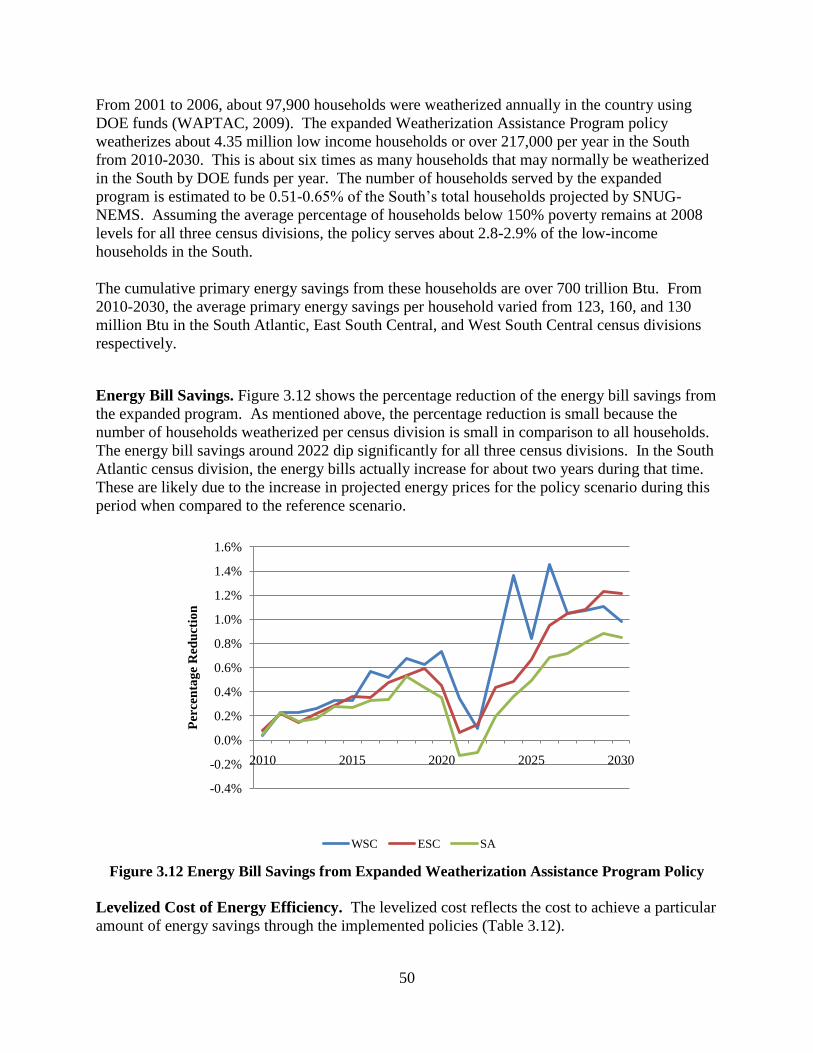
50
From 2001 to 2006, about 97,900 households were weatherized annually in the country using
DOE funds (WAPTAC, 2009). The expanded Weatherization Assistance Program policy
weatherizes about 4.35 million low income households or over 217,000 per year in the South
from 2010-2030. This is about six times as many households that may normally be weatherized
in the South by DOE funds per year. The number of households served by the expanded
program is estimated to be 0.51-0.65% of the South‟s total households projected by SNUG-
NEMS. Assuming the average percentage of households below 150% poverty remains at 2008
levels for all three census divisions, the policy serves about 2.8-2.9% of the low-income
households in the South.
The cumulative primary energy savings from these households are over 700 trillion Btu. From
2010-2030, the average primary energy savings per household varied from 123, 160, and 130
million Btu in the South Atlantic, East South Central, and West South Central census divisions
respectively.
Energy Bill Savings. Figure 3.12 shows the percentage reduction of the energy bill savings from
the expanded program. As mentioned above, the percentage reduction is small because the
number of households weatherized per census division is small in comparison to all households.
The energy bill savings around 2022 dip significantly for all three census divisions. In the South
Atlantic census division, the energy bills actually increase for about two years during that time.
These are likely due to the increase in projected energy prices for the policy scenario during this
period when compared to the reference scenario.
Figure 3.12 Energy Bill Savings from Expanded Weatherization Assistance Program Policy
Levelized Cost of Energy Efficiency. The levelized cost reflects the cost to achieve a particular
amount of energy savings through the implemented policies (Table 3.12).
-0.4%
-0.2%
0.0%
0.2%
0.4%
0.6%
0.8%
1.0%
1.2%
1.4%
1.6%
2010 2015 2020 2025 2030
Per
cen
tag
e R
edu
ctio
n
WSC ESC SA

51
Table 3.12 Levelized Cost of Energy Efficiency from
Expanded Weatherization Assistance Program Policy in 2020
(2007$)
Energy Type Cost of Efficiency
Electricity (¢/kWh) 8.6
Natural Gas (¢/therm) 230
Total Energy ($/MMBtu) 24
The electricity levelized cost for this policy is 8.6¢/kWh in 2007 dollars, which is lower than
most residential retail electricity prices seen in the South, which averaged 8.5-10.5¢/kWh by
census division in 2007 (EIA, 2009g). Since the levelized cost for electricity efficiency is lower
than most retail costs, the electricity efficiency potential from the Expanded Weatherization
Assistance Program policy can be achieved with modest savings in most savings. In 2007, only
four states in the South had retail electricity prices that were lower than the levelized cost for
electricity efficiency. These states were: West Virginia (6.73¢/kWh), Kentucky (7.34¢/kWh),
Tennessee (7.84¢/kWh), and Oklahoma (8.58¢/kWh) (EIA, 2009g).
The natural gas levelized cost for this policy is 230¢/therm, which is also higher than residential
retail natural gas prices seen in the South. In 2007, Southern residential retail prices varied from
120-206¢/therm in the states and DC (EIA, 2009g). The levelized cost of natural gas efficiency
for the expanded Weatherization Assistance Program is higher than all of these prices,
suggesting that the natural gas measures implemented by the policy would not be cost effective
immediately.
As electricity efficiency comprises 50-66% of the total efficiency potential while natural gas
comprises 26-37%, the savings from implementing electricity efficiency measures will likely
offset the costs associated with natural gas efficiency measures.
Economic Tests. The energy bill savings from the policy exceeds the public and private
investment costs associated with the program for the much of their duration (See Figure 3.13).
Due to the relative price increase of the policy scenario around 2022 in comparison to the
reference scenario, the energy bill savings decrease around that duration. Appendix C.3
summarizes the cost and savings calculations for the policy.

52
Figure 3.13 Costs and Savings from Expanded Weatherization Assistance Program Policy
The benefit cost ratio of the net present value benefits and costs is 1.1 for this test. For the
approximate 5.31 million low income households served by the Expanded Weatherization
Assistance Program, the average total discounted cost per home was $1,340 while the total
discounted savings per home was about $1,600. Outside of the calculated savings and costs,
non-energy benefits also accrue from the program and are not included in this calculation.
Table 3.13 Total Resource Test for Expanded Weatherization Assistance Program Policy*
(Million $2007)
B/C Public Costs Private Costs
Total
Discount
Costs
Total
Discount
Savings
Annual Annual Annual Cumulative
Costs
Cumulative
Savings Administration Cost Investment Cost (Investment & Other)
2020 54 486 11.6 3,870 2,180
1.1 2030 54 486 12.8 5,840 4,560
NPV 572 5,150 121 5,840 6,420
*Cumulative Costs and Savings beginning in 2011. NPV included savings post 2030 to until 2050, when the
lifetime of weatherization measures installed in 2030 cease.
Some non-energy benefits experienced by weatherized households include property value
benefits and water and sewage savings. There are also health, safety, and comfort benefits
accrued by residents. Other social, environmental, and economic benefits accrue to society in
general from the weatherization assistance program. For instance, the reduction of bad debt
write-off, fewer service calls, reduction in electricity transmission and distribution losses and
other benefits that reduce utility costs and should indirectly benefit rate payers. Schweitzer and
-$0.2
$0.0
$0.2
$0.4
$0.6
$0.8
$1.0
$1.2
$1.4
2010 2015 2020 2025 2030 2035 2040 2045 2050
Bil
lio
n 0
7$
Public Investment Private Investment Energy Bill Savings

53
Tonn calculated the societal benefit cost ratio to be 3.7, with a range from 2.0 and 52.5, when
including low and high non-energy benefit estimates (2002). Naturally, the benefit to cost ratio
would be even higher than 1.1 if these non-energy benefits were included.
3.3.4 Residential Retrofit Incentive with Equipment Standards
A retrofitting policy can offer greater savings than the weatherization assistance program, since
all new homes are eligible. The Middle Class Task Force found that residential retrofitting may
reduce energy consumption by up to 40% per home (Recovery through Retrofit, 2009).
Residential standards exist for products pertaining to the modeled residential retrofit. These
include central air conditioners, room air conditioners, heat pumps, furnaces, boilers, and water
heaters. Standards for these products were implemented by the National Appliance Energy
Conservation Act of 1987 (ASAP, 2009a).
When households retrofit heating, cooling, or water heating equipment, they have the
opportunity to reduce their monthly costs by increasing their efficiency. New products emerging
on the market can provide greater energy savings without sacrificing performance. For instance,
heat pump water heaters (Figure 3.14) available in late 2009 can cut annual energy costs for
water heating by over 50% (Energy Star, 2009b). These water heaters pull heat from the air to
heat the water. They can be standalone units, like the one shown in Figure 3.14, or they can be
added to existing conventional storage water heaters as a retrofit measure (DOE/EERE, 2009d).
The higher upfront costs for a standalone unit are estimated to be paid back by energy savings in
about three years (Energy Star, 2009b).
Figure 3.14: Heat Pump Water Heater (Lapsa, 2009)
Policy Description and Modeling. This policy includes a retrofit program for heating, cooling,
and water heating, as well as standards for furnaces, heat pumps, air-conditioners, and water
heaters. The retrofit program includes an incentive measure for 30% of capital cost for the most
efficient technologies available.

54
The residential subsidy for efficient retrofit appliances was implemented by making changes to a
residential input file in SNUG-NEMS detailing appliance efficiencies and costs. Only
equipment classes that have a projected efficiency improvement during the study period received
the subsidy for the highest efficiency equipment within the class. For these, a 30% reduction in
their capital cost was given.
A federal equipment standard is assumed to be adopted by all states as required by federal rule.
This standard was implemented in SNUG-NEMS in the same input file as the incentives. When
a standard was implemented, the least efficient grouping of equipment was removed from the
market. Every ten years, the lowest efficiency equipment remaining was removed (See
Appendix C-2.2 for additional information on standard implementation).
Table 3.14 lists the equipment affected by the incentives, standards, and the year of standard
implementation. See Appendix C-2.2 for additional information on the equipment incentives,
standards, and dates.
Table 3.14 Equipment Affected by
Residential Retrofit Incentives and Equipment Standards*
Equipment Classes 30% Incentive Equipment Standard
Implementation Year*
Electric Heat Pump Heat Pump 4 Heat Pump 1 & 2 (2014)
Natural Gas Furnace Furnace 5 Furnace 1, 2, & 3 (2014)
Natural Gas Radiator Radiator 3 Radiator 1 & 2 (2013)
Kerosene Furnace Furnace 3 Furnace 1 & 2 (2015)
LPG Furnace Furnace 5 Furnace 1, 2, & 3 (2015)
Distillate Furnace Furnace 3 Furnace 1 & 2 (2015)
Distillate Radiator Radiator 3 Radiator 1 & 2 (2013)
Geothermal Heat Pump Heat Pump 2 Heat Pump 1 (2014)
Natural Gas Heat Pump --- Heat Pump (2014)
Room Air Conditioner Room ACs 2 & 3* Room AC 1 (2006)*
Central Air Conditioner Central AC 4 Central AC 1 & 2 (2014)
Natural Gas Water Heater Water Heater 4 Water Heater 1 & 2 (2013)
Electric Water Heater Water Heater 5 Water Heater 1, 2, & 3 (2013)
Distillate Water Heater Water Heater 3 Water Heater 1 &2 (2013)
LPG Water Heater Water Heater 4 Water Heater 1 & 2 (2013) *See Appendix C.2.2 for additional details.
Technology Demand Shifts. The Residential Retrofit Incentives and Equipment Standards
Policy causes demand changes for energy efficient technologies. The policy causes a shift
towards higher efficiency equipment, as can be expected, in heating, cooling, and water heating
end-uses. Table 3.15 lists examples of equipment, their efficiencies, and their percentage of use
in the reference and policy scenarios to show how technology demand has shifted. See
Appendix C.2.2 for additional technologies. The numbers listed in the efficiency column are
derived from the SNUG-NEMS input file.

55
Table 3.15 Total Technology Demand Shifts from
Residential Retrofit Incentives and Equipment Standards Policy
Description Efficiency Reference Policy
2020 2030 2020 2030 2020 2030
Central Air 4.69 --- 29% 33% 35% 0%
6.74 --- 6% 7% 65% 100%
Natural Gas Furnace 0.90 0.90 40% 35% 41% 0%
0.96 0.96 12% 12% 59% 100%
Electric Water Heater 2.30 --- 4% 10% 40% 0%
2.40 --- 0% 0% 60% 100%
Energy Savings. The policy saves over 26,800 trillion Btu of primary energy over the duration
of the implemented measures, which last until 2050. Table 3.16 shows the primary energy
savings in trillion Btu from the policy by census division. These values vary from division to
division, with the largest savings attributed to the South Atlantic census division, which includes
the most states. Retrofit measures are assumed to have a lifetime of 20 years, so even though
investsments discontinue after 2030, the savings from the investments persist until 2050.
Table 3.16 Primary Energy Savings from Residential Retrofit
Incentives & Equipment Standards Policy (TBtu)
WSC ESC SA Total
2020 211 107 421 739
2030 355 177 777 1,310
Cumulative to 2050 7,380 3,720 15,700 26,800 *Primary energy savings is the energy required to generate the avoided energy.
Figure 3.15 shows the percentage reduction of primary energy savings attributed to the policy in
each census division in 2020 and 2030. The percentage reduction due to the policy increases
from over time. For the South Atlantic region, it rises from 8.56% in 2020 to 13.8% reduction in
2030.

56
Figure 3.15 Primary Energy Savings for Residential Retrofit Incentives
and Equipment Standards Policy
The SNUG-NEMS modeling of this policy applies to both retrofit and new homes. Though the
policy is mostly applied to retrofits, about a quarter of the efficient equipment attributable to the
policy are not retrofit applications. The results presented here does not separate the savings
between retrofit and new applications. Because of this, the savings and costs attributed to the
Retrofit Incentives and Equipment Standards policy may be inflated.
Levelized Cost of Energy Efficiency. The electricity levelized cost for this policy is 3.4¢/kWh (noted in Table 3.17), which is lower
than the residential retail electricity prices seen in the South. In 2007, Southern residential retail
prices averaged 8.5-10.5¢/kWh by census division (EIA, 2009g). As the levelized cost for
electricity efficiency is much lower than the retail cost, the electricity efficiency potential from
the residential retrofit policy can likely be achieved economically.
Table 3.17 Levelized Cost of Energy Efficiency from Residential
Retrofit Incentives and Equipment Standards Policy in 2020
Energy Type Cost of Efficiency
Electricity (¢/kWh) 3.4
Natural Gas (¢/therm) 110
Total Energy ($/MMBtu) 11
The natural gas levelized cost for this policy is 110¢/therm, which is also lower than residential
retail natural gas prices seen in the South. In 2007, Southern residential retail prices ranged from
120-206¢/therm by state (EIA, 2009g). This indicates that every therm of natural gas saved
through the efficiency measures from this policy is and will likely continue to be cheaper to
implement than continuing previous consumption habits by using that therm. In general, this
7.4%
11%
6.4%
9.6%8.6%
14%
0%
2%
4%
6%
8%
10%
12%
14%
16%
2020 2030
Per
cen
tag
e R
edu
ctio
n
WSC ESC SA

57
policy can provide energy efficiency savings economically since natural gas and electricity
efficiency potential dominate the efficiency potential from the policy.
Energy Bill Savings. Figure 3.16 shows the percentage reduction in energy bill savings from
this retrofit policy. The percentage reduction increases over time, going from zero in 2010 to
about 16-18% reduction in 2030, depending on the census division.
Figure 3.16 Energy Bill Savings from Residential Retrofit Incentives
and Equipment Standards Policy
Economic Tests. Energy bill savings due to this policy increase steadily over the duration of the
policy and are assumed to decrease linearly until 2050, after the 20 year lifetime assumed for
retrofit measures. Figure 3.17 shows the public and private investment trends from retrofits,
which are similar up to about 2025 when public costs then jump upwards. Larger public subsidy
outlays for increased purchases of highly efficient equipment occur around 2025, prompted by
equipment standards that remove cheaper, but less efficient models from the market. The energy
bill savings from the policy exceeds the public and private investment. Appendix C.3 details the
cost calculations for the policy.
0%
2%
4%
6%
8%
10%
12%
14%
16%
18%
20%
2010 2015 2020 2025 2030
Per
cen
tag
e R
edu
ctio
n
WSC ESC SA

58
Figure 3.17 Costs and Savings from Residential Retrofit and Equipment Standards Policy
The equipment implemented by the program is estimated to have a twenty year life. Therefore,
savings from the program continue to accrue until 2050 even though all costs cease in 2030. The
benefit cost ratio is 1.4, suggesting that benefits from this policy are 1.4 times greater than the
associated costs.
Table 3.18 Total Resource Test for Residential Retrofit and Equipment Standards Policy*
(Million $2007)
B/C Public Costs Private Costs
Total
Discount
Costs
Total
Discount
Savings
Annual Annual Annual Cumulative
Costs
Cumulative
Savings Administration Cost Investment Cost (Investment & Other)
2020 1.43 5,360 4,350 46,700 26,100
1.4 2030 1.43 8,800 3,420 86,600 84,400
NPV 15.1 52,300 34,300 86,600 119,000
*Cumulative Costs and Savings beginning in 2011. NPV included savings post 2030 to until 2050, when retrofit
measures implemented in 2030 reached the end of the assumed 20 year life.
3.4 INTEGRATED RESIDENTIAL POLICIES
The remainder of this chapter describes the analysis of combining all the residential policies:
Residential Building Codes with Third Party Verification, Appliance Incentives and Standards,
Expanded Weatherization Assistance Program, and Residential Retrofit Incentives and
Equipment Standards. Due to the synergistic effects of SNUG-NEMS modeling, the integrated
results will not be the sum of the previous single policy results.
$0
$5
$10
$15
$20
$25
2010 2015 2020 2025 2030 2035 2040 2045 2050
Bil
lio
n 0
7$
Public Investment Private Investment Energy Bill Savings
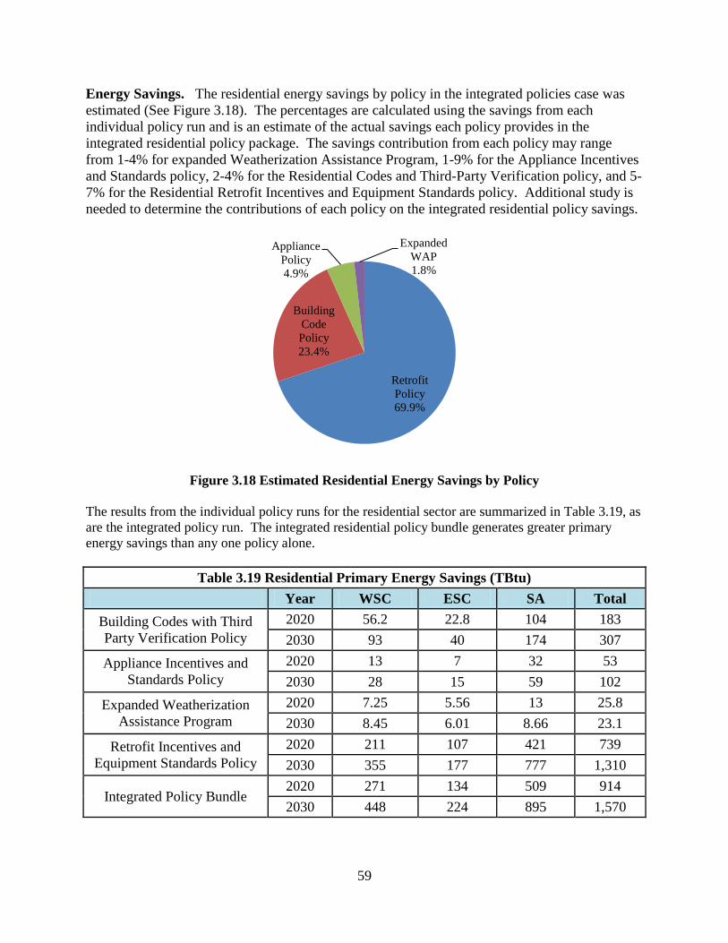
59
Energy Savings. The residential energy savings by policy in the integrated policies case was
estimated (See Figure 3.18). The percentages are calculated using the savings from each
individual policy run and is an estimate of the actual savings each policy provides in the
integrated residential policy package. The savings contribution from each policy may range
from 1-4% for expanded Weatherization Assistance Program, 1-9% for the Appliance Incentives
and Standards policy, 2-4% for the Residential Codes and Third-Party Verification policy, and 5-
7% for the Residential Retrofit Incentives and Equipment Standards policy. Additional study is
needed to determine the contributions of each policy on the integrated residential policy savings.
Figure 3.18 Estimated Residential Energy Savings by Policy
The results from the individual policy runs for the residential sector are summarized in Table 3.19, as
are the integrated policy run. The integrated residential policy bundle generates greater primary
energy savings than any one policy alone.
Table 3.19 Residential Primary Energy Savings (TBtu)
Year WSC ESC SA Total
Building Codes with Third
Party Verification Policy
2020 56.2 22.8 104 183
2030 93 40 174 307
Appliance Incentives and
Standards Policy
2020 13 7 32 53
2030 28 15 59 102
Expanded Weatherization
Assistance Program
2020 7.25 5.56 13 25.8
2030 8.45 6.01 8.66 23.1
Retrofit Incentives and
Equipment Standards Policy
2020 211 107 421 739
2030 355 177 777 1,310
Integrated Policy Bundle 2020 271 134 509 914
2030 448 224 895 1,570
Retrofit
Policy
69.9%
Building
Code
Policy
23.4%
Appliance
Policy
4.9%
Expanded
WAP
1.8%
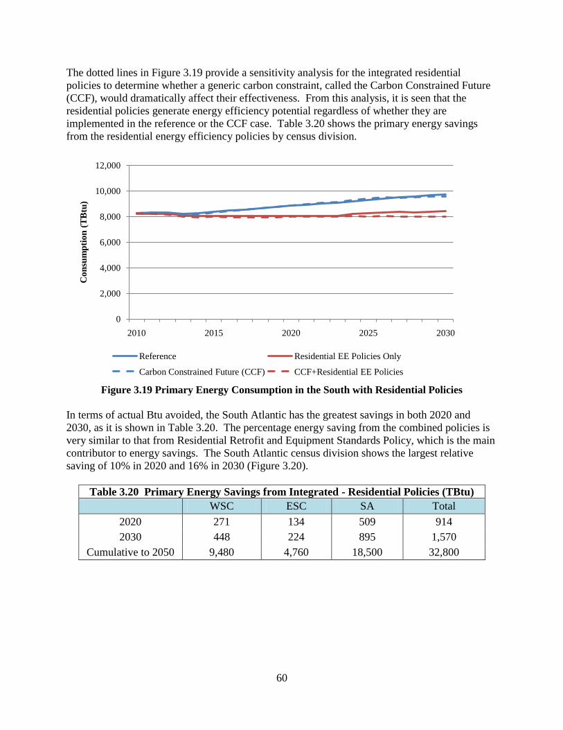
60
The dotted lines in Figure 3.19 provide a sensitivity analysis for the integrated residential
policies to determine whether a generic carbon constraint, called the Carbon Constrained Future
(CCF), would dramatically affect their effectiveness. From this analysis, it is seen that the
residential policies generate energy efficiency potential regardless of whether they are
implemented in the reference or the CCF case. Table 3.20 shows the primary energy savings
from the residential energy efficiency policies by census division.
Figure 3.19 Primary Energy Consumption in the South with Residential Policies
In terms of actual Btu avoided, the South Atlantic has the greatest savings in both 2020 and
2030, as it is shown in Table 3.20. The percentage energy saving from the combined policies is
very similar to that from Residential Retrofit and Equipment Standards Policy, which is the main
contributor to energy savings. The South Atlantic census division shows the largest relative
saving of 10% in 2020 and 16% in 2030 (Figure 3.20).
Table 3.20 Primary Energy Savings from Integrated - Residential Policies (TBtu)
WSC ESC SA Total
2020 271 134 509 914
2030 448 224 895 1,570
Cumulative to 2050 9,480 4,760 18,500 32,800
0
2,000
4,000
6,000
8,000
10,000
12,000
2010 2015 2020 2025 2030
Co
nsu
mp
tio
n (
TB
tu)
Reference Residential EE Policies Only
Carbon Constrained Future (CCF) CCF+Residential EE Policies
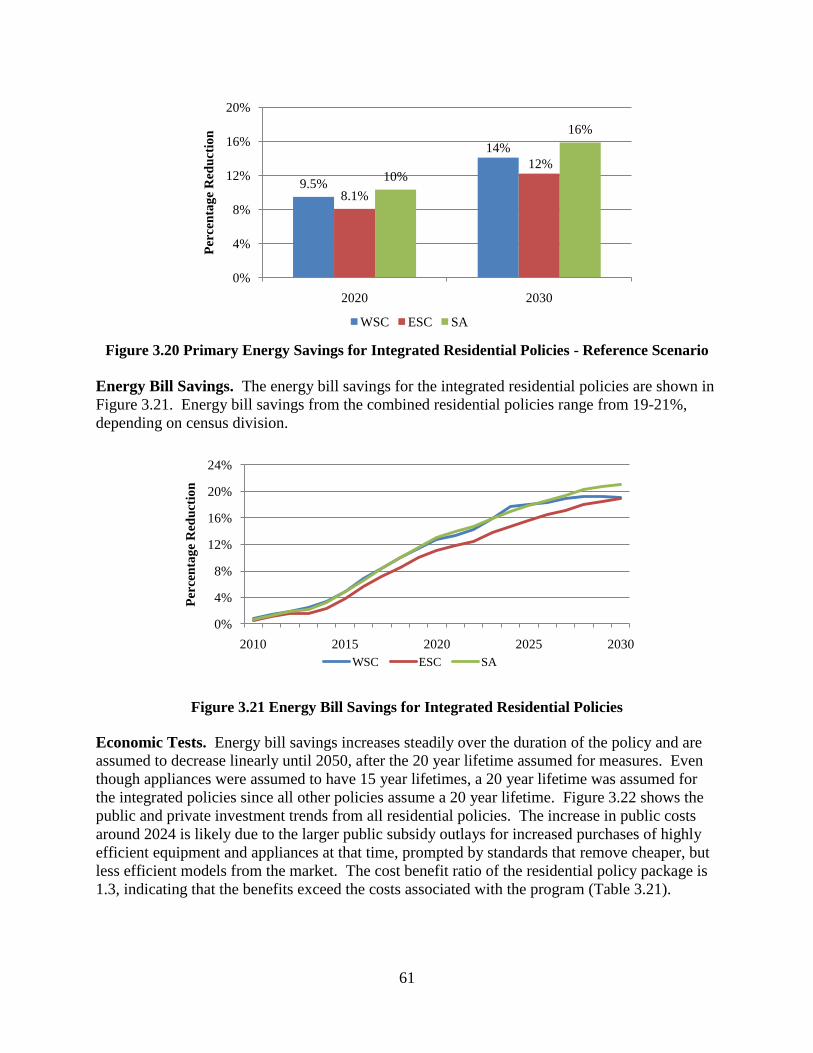
61
Figure 3.20 Primary Energy Savings for Integrated Residential Policies - Reference Scenario
Energy Bill Savings. The energy bill savings for the integrated residential policies are shown in
Figure 3.21. Energy bill savings from the combined residential policies range from 19-21%,
depending on census division.
Figure 3.21 Energy Bill Savings for Integrated Residential Policies
Economic Tests. Energy bill savings increases steadily over the duration of the policy and are
assumed to decrease linearly until 2050, after the 20 year lifetime assumed for measures. Even
though appliances were assumed to have 15 year lifetimes, a 20 year lifetime was assumed for
the integrated policies since all other policies assume a 20 year lifetime. Figure 3.22 shows the
public and private investment trends from all residential policies. The increase in public costs
around 2024 is likely due to the larger public subsidy outlays for increased purchases of highly
efficient equipment and appliances at that time, prompted by standards that remove cheaper, but
less efficient models from the market. The cost benefit ratio of the residential policy package is
1.3, indicating that the benefits exceed the costs associated with the program (Table 3.21).
9.5%
14%
8.1%
12%10%
16%
0%
4%
8%
12%
16%
20%
2020 2030
Per
cen
tag
e R
edu
ctio
n
WSC ESC SA
0%
4%
8%
12%
16%
20%
24%
2010 2015 2020 2025 2030
Per
cen
tag
e R
edu
ctio
n
WSC ESC SA

62
Figure 3.22 Costs and Savings from the Integrated Residential Policies
Table 3.21 Total Resource Test for Integrated Residential Policies*
(Million $2007)
B/C Public Costs Private Costs
Total
Discount
Costs
Total
Discount
Savings
Annual Annual Annual Cumulative
Costs
Cumulative
Savings Administration Cost Investment Cost (Investment & Other)
2020 548 7,540 4,120 65,600 35,900
1.3 2030 648 12,100 2,870 115,000 104,000
NPV 5,760 75,300 33,600 115,000 143,000
*Cumulative Costs and Savings beginning in 2011. NPV included savings post 2030.
$0
$5
$10
$15
$20
$25
$30
2010 2015 2020 2025 2030 2035 2040 2045 2050
Bil
lio
n 0
7$
Public Investment Private Investment Energy Bill Savings

63
3.5 SUMMARY AND DISCUSSION OF RESULTS FOR THE RESIDENTIAL SECTOR
This analysis of residential efficiency potential suggests that the South could save 9.7% of the
energy it is forecasted to consume in the residential sector in 2020 and 15% in 2030 by
implementing this collection of four policies. Table 3.22 gives a summary of the net present
cost, benefit, and benefit cost ratio from the residential policies and integrated policy bundle.
Table 3.22 Total Resource Cost Tests by Sector (Million 07$)
Residential Sector Policies
Building
Codes with
Third-Party
Verification
Appliances
Incentives
&
Standards
Expanded
Weatherization
Assistance
Program
Retrofit
Incentives
&
Equipment
Standards
Integrated
Residential
Policies
NPV Cost $7,280 $25,500 $5,840 $86,600 $115,00
NPV Benefit $40,900 $7,060 $6,420 $119,000 $143,000
B/C Ratio 5.6 0.3 1.1 1.4 1.3
3.5.1 Comparison with Other Studies
Over the past decade, numerous state and regional studies have examined the potential for
energy efficiency improvements in the South (the results of several key studies are summarized
in Figure 3.23). Based on a review of 19 of these, focusing on estimates for 2020, Chandler and
Brown (2009) concluded that 800 TBtu of residential energy (or 9% of the residential
consumption forecast for 2020) could be cost-effectively avoided with aggressive, but feasible
policies. Since that study was published, McKinsey and Company (2009) completed a national
analysis of the “NPV-positive potential for energy efficiency,” including a breakdown of results
for the South and individual sectors. The estimate of energy efficiency potential in the South‟s
residential sector in 2020 from the McKinsey study is 26%.
This study‟s estimate for residential efficiency potential is essentially identical to the estimate
for Appalachia (Brown, et al., 2009), which included many of the Southern states and involved a
similar analytic approach. Our result is comparable to the moderate scenario in the IWG (2000)
study of the nation, but is substantially less than that study‟s advanced scenario. A significant
portion of the residential savings from both the McKinsey and IWG studies are attributable to
improved lighting technologies (about 16% in the case of McKinsey). Yet lighting was excluded
from the residential estimate in this study because most of its potential savings have now been
legislated through lighting standards and have been subtracted from the baseline forecast of
future consumption. It is likely if lighting had been included in this study, the estimated energy
efficiency potential within the residential sector might have increased by 1-2%.

64
Figure 3.23 Comparison of Residential Energy Savings Estimates Across Studies
EPRI (2009) provides an estimate of residential electricity efficiency potential for the South in
2030. The realistic potential for efficiency is estimated to be 5%, and the maximum potential is
larger at 8%. These estimates are considerably smaller because they only take into account the
reduction in electricity consumption that could occur as the result of programs run by electric
utilities. As a result, they do not include the potential savings from building codes or appliance
standards (Personal Communication with Ammi Amarnath, Electric Power Research Institute,
December 10, 2009). No comparison of overall estimates in 2030 was conducted due to the
limited number of studies that provided estimates for that year.
3.5.2 Limitations and Needs for Future Research
This analysis of energy efficiency potential in the residential sector in the South has several
limitations that require further analysis and research than was possible in this project.
Specifically, the analysis could be improved in several ways.
A. Include more technology options, especially emerging technologies, to better model
the energy efficiency potential. The technology profiles included in the SNUG-NEMS
input files are limited and in some cases do not reflect the most recent advancements.
For instance, integrated heat pump systems are not included in the residential
technologies, despite existing commercialization activities. This limits the technology
options available for incentives and standards. The residential retrofit policy only
incentivized 13 technologies and only implemented standards for 18 technologies.
Greater technology options would allow for more realistic modeling of the energy
efficiency potential.
B. Account for household behavioral effects to identify a wider range of energy
efficiency potential. SNUG-NEMS employs price elasticities of demand that result in
0%
5%
10%
15%
20%
25%
30%
Energy
Efficiency in the
South (2010)
Chandler and
Brown (2009)
Brown et al.
(2009)
IWG (2000)
Moderate
IWG (2000)
Advanced
McKinsey
(2009)
Per
cen
tag
e S
av
ing
s
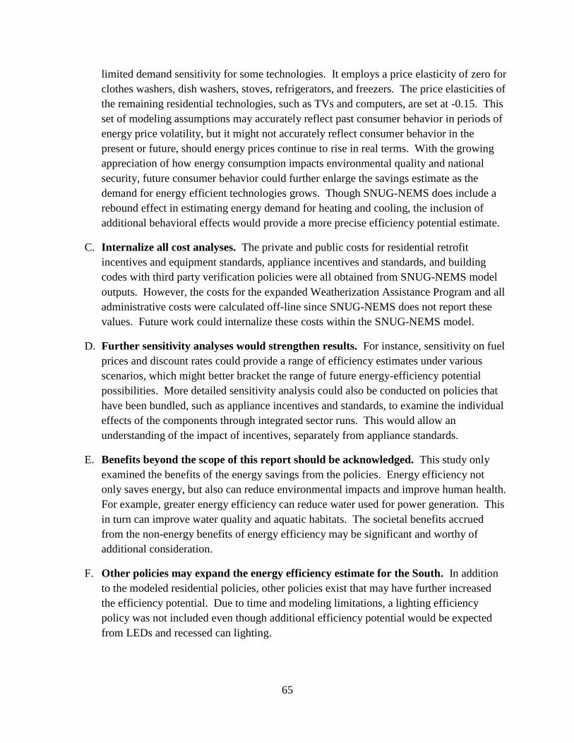
65
limited demand sensitivity for some technologies. It employs a price elasticity of zero for
clothes washers, dish washers, stoves, refrigerators, and freezers. The price elasticities of
the remaining residential technologies, such as TVs and computers, are set at -0.15. This
set of modeling assumptions may accurately reflect past consumer behavior in periods of
energy price volatility, but it might not accurately reflect consumer behavior in the
present or future, should energy prices continue to rise in real terms. With the growing
appreciation of how energy consumption impacts environmental quality and national
security, future consumer behavior could further enlarge the savings estimate as the
demand for energy efficient technologies grows. Though SNUG-NEMS does include a
rebound effect in estimating energy demand for heating and cooling, the inclusion of
additional behavioral effects would provide a more precise efficiency potential estimate.
C. Internalize all cost analyses. The private and public costs for residential retrofit
incentives and equipment standards, appliance incentives and standards, and building
codes with third party verification policies were all obtained from SNUG-NEMS model
outputs. However, the costs for the expanded Weatherization Assistance Program and all
administrative costs were calculated off-line since SNUG-NEMS does not report these
values. Future work could internalize these costs within the SNUG-NEMS model.
D. Further sensitivity analyses would strengthen results. For instance, sensitivity on fuel
prices and discount rates could provide a range of efficiency estimates under various
scenarios, which might better bracket the range of future energy-efficiency potential
possibilities. More detailed sensitivity analysis could also be conducted on policies that
have been bundled, such as appliance incentives and standards, to examine the individual
effects of the components through integrated sector runs. This would allow an
understanding of the impact of incentives, separately from appliance standards.
E. Benefits beyond the scope of this report should be acknowledged. This study only
examined the benefits of the energy savings from the policies. Energy efficiency not
only saves energy, but also can reduce environmental impacts and improve human health.
For example, greater energy efficiency can reduce water used for power generation. This
in turn can improve water quality and aquatic habitats. The societal benefits accrued
from the non-energy benefits of energy efficiency may be significant and worthy of
additional consideration.
F. Other policies may expand the energy efficiency estimate for the South. In addition
to the modeled residential policies, other policies exist that may have further increased
the efficiency potential. Due to time and modeling limitations, a lighting efficiency
policy was not included even though additional efficiency potential would be expected
from LEDs and recessed can lighting.

66
These limitations suggest the presented estimate of residential energy efficiency potential is
conservative because it does not include certain behavioral effects, estimates for lighting, the full
range of technologies, environmental benefits, and other possible policies.
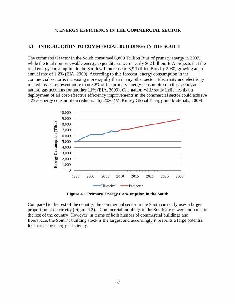
67
4. ENERGY EFFICIENCY IN THE COMMERCIAL SECTOR
4.1 INTRODUCTION TO COMMERCIAL BUILDINGS IN THE SOUTH
The commercial sector in the South consumed 6,800 Trillion Btus of primary energy in 2007,
while the total non-renewable energy expenditures were nearly $62 billion. EIA projects that the
total energy consumption in the South will increase to 8,9 Trillion Btus by 2030, growing at an
annual rate of 1.2% (EIA, 2009). According to this forecast, energy consumption in the
commercial sector is increasing more rapidly than in any other sector. Electricity and electricity
related losses represent more than 80% of the primary energy consumption in this sector, and
natural gas accounts for another 11% (EIA, 2009). One nation-wide study indicates that a
deployment of all cost-effective efficiency improvements in the commercial sector could achieve
a 29% energy consumption reduction by 2020 (McKinsey Global Energy and Materials, 2009).
Figure 4.1 Primary Energy Consumption in the South
Compared to the rest of the country, the commercial sector in the South currently uses a larger
proportion of electricity (Figure 4.2). Commercial buildings in the South are newer compared to
the rest of the country. However, in terms of both number of commercial buildings and
floorspace, the South‟s building stock is the largest and accordingly it presents a large potential
for increasing energy-efficiency.
0
1,000
2,000
3,000
4,000
5,000
6,000
7,000
8,000
9,000
10,000
1995 2000 2005 2010 2015 2020 2025 2030
En
erg
y C
on
sum
pti
on
(T
Btu
)
Historical Projected

68
Figure 4.2 Commercial Energy Source by Fuel in 2007 (EIA,2009)
A number of commercial efficiency programs exist in the South. Maryland and Washington DC
have adopted state-specific commercial appliance standards for equipment that is not covered by
federal standards. Several states, such as Alabama, Florida, North Carolina, and Virginia have
policies that promote energy efficiency in public buildings through retrofitting programs (U.S.
Environmental Protection Agency 2008). Table 4.1 shows the number of commercial building
and floorspace that they represent in the South.
Table 4.1 Commercial Buildings in the South by Building Type, 2003
Number of Buildings
(thousands)
Total Floorspace
(million square feet)
Principal Building
Activity 156 3,983
Education 94 487
Food Sales 127 764
Food Service 48 1,277
Health Care 100 2,970
Lodging 295 5,094
Mercantile 545 8,877
Office 92 1,174
Public Assembly 15 373
Public Order and Safety 158 1,498
Religious Worship 198 1,358
Service 277 3,966
Warehouse and Storage 21 Q
Other 88 701
(CBECS, 2003)
Liquid
Fuels
Subtotal2%
Natural
Gas
11%Other
1%
Renewabl
es
0%
Electricity
28%Electricity
Related
Losses
58%
South
Liquid
Fuels
Subtotal2%
Natural
Gas
16%
Other
4%
Renewable
s
1%
Electricity
24%Electricity
Related
Losses53%
United States

69
4.2 BARRIERS TO COMMERCIAL ENERGY EFICIENCY AND POLICY OPTIONS
4.2.1 Barriers to Energy-Efficiency in Commercial Buildings
Energy-efficient commercial buildings are seen by many experts to be one of the most cost-
effective strategies for cutting energy costs and curbing carbon emissions (McKinsey &
Company, 2009, p. xii; National Academy of Sciencs, 2009). However, for a variety of reasons,
developers, building owners, and tenants typically under invest in these “NPV-positive”
improvements.
The large, diverse, and fragmented nature of the buildings industry helps explain some of this
underinvestment. Developers, architects, engineering firms, leasing agents, and many others
influence the design and construction of commercial buildings, and they often do not represent
the long-term interests of building owners and occupants (CCCSTI, 2009; Brown et al., 2009).
This market structure results in an overemphasis on minimizing first costs, meaning that owners
and occupants are saddled with higher operating costs, including energy bills.
Once a commercial building is built, the landlord-tenant relationship becomes a disincentive for
energy upgrades (Murtishaw and Sathaye, 2006). When the tenants pay the energy bill, the
landlord is not incentivized to invest in efficient equipment. The situation that favors the
purchase of efficient equipment (when the landlord pays the utility bill) leads to a disincentive
for the tenants to use energy wisely (Ottinger and Williams, 2002). Since 51% of
nongovernment-owned commercial buildings are rented or leased (DOE, 2008, Table 1.3.8),
commercial buildings are particularly prone to this problem of misplaced incentives.
In the buildings industry, there is also a workforce training gap. Many architects, engineers,
builders and tradespeople do not have access to sufficient training in new technologies, new
standards, new regulations, and best practices. Lowe and Oreszczyn (2008) describe this lack of
knowledge as a remnant of the shift of the construction industry from one of apprenticeship to
one of labor, and they suggest that the industry will need to become a producer of human capital
in order to support a new generation of buildings. Local government authorities tend to face this
gap as well with building code officials working without skills necessary to evaluate compliance
with building energy codes.
The result of these (and many other) market barriers and obstacles is a large reservoir of lost
opportunities for improving the energy efficiency of U.S. buildings.
4.2.2 Policy Options to Improve Energy-Efficiency in the Commercial Sector
This study evaluates two policies15
to improve energy efficiency in commercial buildings and
appliances in the South: Aggressive Commercial Appliance Standards, wherein more stringent
15
Originally, there was a third policy, Commercial Building Codes, which has been advocated for in a number of
studies. However, after preliminary modeling, the energy efficiency gains from reduced heating were fully offset by
increased cooling. After discussing this with a number of experts (North Carolina State Energy Office, Oak Ridge
National Laboratory, and Energy Information Agency), we determined that using SNUG-NEMS to model tighter
commercial building shells would not show efficiency improvements because of the increased internal heat gains
from lighting and electronic equipment that would require air conditioning.

70
appliance standards are implemented; and Incentivizing HVAC Retrofits, where customers are
encouraged to upgrade their current appliances with higher efficient ones. These polices, as with
most of those in other chapters, are envisioned as being more aggressive than existing programs
but are anticipated to be no cost or low cost. For the purposes of this study, these policies are
implemented across the South uniformly. However, the way these policies would actually be
implemented may vary and would conform to the specific goal and capacity of each policy
making body (local, state, or federal). Table 4.2 shows some supporting actions and policies that
states may wish to pursue in conjunction with or instead of the policies described in this report.
The relevance of this analysis should extend beyond the potential of implementing these
particular policies. Rather these policies are general enough that a range of potential
implementations could attain the energy and economic effects by reaching similar levels of
avoided energy consumption.
Table 4.2 Policy Actions that Support Commercial Energy Efficiency
Actions HVAC Retrofit Policy Aggressive Commercial Equipment
Standards
Research, Development,
and Demonstration
Development of new insulation,
heating, and cooling technologies
useful for the local climate
Support for research and development
for innovation in appliance
performance
Financing
Low or no-interest loans for
incremental cost of improvements for
existing buildings
Efficiency Grants
Enable performance contracting
Low or no-interest loans for ENERGY
STAR equipment
Enable performance contracting
Financial Incentives
Incremental cost incentives for efficient
retrofits
Tax credits for efficient purchases
Incentives to use efficiency features
and lower consumption
Tax credits for efficient purchases
Equipment buyback programs
Regulations NA
Tighter office equipment standards
Tighter equipment standards
Standby efficiency standards
Information
Dissemination & Training
Training Architects, Builders,
Contractors, and Building Managers
Public awareness campaigns to inform
consumers of the benefits of
conservation and efficiency measures.
Awareness campaigns to inform
executives of the benefits of efficiency
measures
Advanced metering or billing methods
Awareness campaigns to inform
executives of the benefits of
conservation and efficiency measures
Advanced metering and billing
Procurement Government lead by example
procurement programs
Government lead by example
procurement programs
Capacity Building
Centers for energy efficiency to train
next generation of architects, builders,
retrofitters
N/A
This table describes policy actions available that could further the savings from the policy packages modeled in
this study. The policy actions shown in italics are modeled in this study, while the others are not.
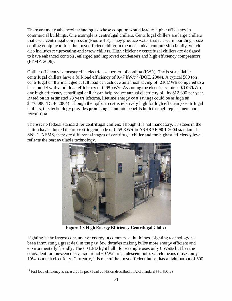
71
There are many advanced technologies whose adoption would lead to higher efficiency in
commercial buildings. One example is centrifugal chillers. Centrifugal chillers are large chillers
that use a centrifugal compressor (Figure 4.3). They produce water that is used in building space
cooling equipment. It is the most efficient chiller in the mechanical compression family, which
also includes reciprocating and screw chillers. High efficiency centrifugal chillers are designed
to have enhanced controls, enlarged and improved condensers and high efficiency compressors
(FEMP, 2006).
Chiller efficiency is measured in electric use per ton of cooling (kW/t). The best available
centrifugal chillers have a full-load efficiency of 0.47 kW/t16
(DOE, 2004). A typical 500 ton
centrifugal chiller managed at full load can achieve an annual saving of 210MWh compared to a
base model with a full load efficiency of 0.68 kW/t. Assuming the electricity rate is $0.06/kWh,
one high efficiency centrifugal chiller can help reduce annual electricity bill by $12,600 per year.
Based on its estimated 23 years lifetime, lifetime energy cost savings could be as high as
$170,000 (DOE, 2004). Though the upfront cost is relatively high for high efficiency centrifugal
chillers, this technology provides promising economic benefits both through replacement and
retrofitting.
There is no federal standard for centrifugal chillers. Though it is not mandatory, 18 states in the
nation have adopted the more stringent code of 0.58 KW/t in ASHRAE 90.1-2004 standard. In
SNUG-NEMS, there are different vintages of centrifugal chiller and the highest efficiency level
reflects the best available technology.
Figure 4.3 High Energy Efficiency Centrifugal Chiller
Lighting is the largest consumer of energy in commercial buildings. Lighting technology has
been innovating a great deal in the past few decades making bulbs more energy efficient and
environmentally friendly. The 60 LED light bulb, for example uses only 6 Watts but has the
equivalent luminescence of a traditional 60 Watt incandescent bulb, which means it uses only
10% as much electricity. Currently, it is one of the most efficient bulbs, has a light output of 300
16
Full load efficiency is measured in peak load condition described in ARI standard 550/590-98

72
lumens and a warm light temperature of 3000K. Though the upfront cost to replace regular
bulbs with this high efficiency one is relatively high, it has a long lifespan of 35,000 hours of
Pharox 60 (compared to an average of 1,000 hours of incandescent bulb), which may make the
payback attractive for some segments of consumers.
Figure 4.4 High Energy Efficiency LED light Bulb
(Source: www.inhabitate.com/2009)

73
4.3 MODELED ENERGY EFFICIENCY POLICIES FOR COMMERCIAL SECTOR
4.3.1 Commercial Appliance Standards
Minimum energy efficiency standards for many major appliances were first established by the
U.S. Congress in Part B of Title III of the Energy Policy and Conservation Act (EPCA), as
amended by the National Energy Conservation Policy Act, by the National Appliance Energy
Conservation Act, by the National Appliance Energy Conservation Amendments of 1988, by the
Energy Policy Act of 1992, by the Energy Policy of 2005 (DOE, 2009a) and by Energy
Independence and Security Act of 2007. These laws and regulations set energy conservation
standards for commercial heating, air conditioning, and water heater equipment (42 U.S.C.
6313(a)). Specifically, the statutes set standards for small, large, and very large commercial
package air conditioning and heating equipment, packaged terminal air conditioners, packaged
terminal heat pumps, warm-air furnaces, packaged boilers, storage water heaters, and unfired hot
water storage tanks. For these types of equipment, the laws and regulations established federal
energy conservation standards that generally correspond to the levels set in the American Society
of Heating, Refrigeration, and Air-Conditioning Engineers (ASHRAE) Standard 90.1 (DOE,
2009b)
EPCA directs DOE to consider amending the existing federal energy efficiency standard for each
type of equipment listed, each time ASHRAE Standard 90.1 is amended with respect to such
equipment (42 U.S.C. 6313(a)(6)(A)). For each type of equipment, EPCA directs that DOE must
adopt amended standards at the new efficiency level in ASHRAE Standard 90.1 (DOE, 2009c).
The latest version of ASHRAE Standard is ASHRAE Standard 90.1-2007, and it was approved
for distribution and officially released to the public on January 10, 2008. Federal energy
efficiency standards generally preempt state laws or regulations except in the case that DOE
grants a waiver of Federal preemption (DOE, 2008) for a particular state law. As of 2009, the
only state that has filed a petition is California. However, states are allowed to develop their own
commercial appliance standards for any equipment that is not covered under federal standards.
Commercial Appliance Standards in the South. Required by federal rule, all states adopt
federal energy efficiency standards. California has successfully petitioned to implement
standards that are more stringent than federal standard for five commercial appliances. In the
South, state standards are not as vigorous as in other regions such as New England.
Maryland and Washington DC are the only southern entities which have adopted their own
standards for commercial appliances. Maryland has standards for Reach-In Refrigerators and
Freezers, Commercial Air Conditioner, Commercial Clothes Washers, Unit Heaters, Hot Food
Holding Cabinets and Water Dispensers. Washington DC has its own commercial appliance
standards for Walk-In Refrigerators and Freezers, Hot Food Holding Cabinets and Water
Dispensers (ASAP, 2009b). However, these standards have been superseded by or will be
superseded by federal standards that are scheduled to be put in place in the next few years.
Compared to residential appliance standards, federal standards for commercial appliances are
less well developed. As there is ample opportunities to achieve meaningful energy efficiency
savings through improving commercial appliances standard. This study develops a set of

74
stringent commercial appliance standard to cover many commercial end uses where there is no
existing federal standard.
Aggressive Commercial Appliance Standards. The definition of our standard policy is the
aggressive implementation of cost effective commercial appliance standards in the South.
Previous studies of similar policies, though with different geographical focus, show significant
energy and energy bill savings and indicate the cost-effectiveness of appliance standards. With a
national model of energy savings using appliance and equipment standards, Rosenquist et.al
identified 12,000 Trillion Btu nationwide of cumulative primary energy saving during the 2010-
2030 period. They note that potential energy bill savings from commercial sector standards have
a greater net present value than those from the residential sector (Rosenquist et.al., 2005).
Another analysis, Energy Efficiency in Appalachia, identified an energy saving potential in 2030
of 143 trillion Btu in the Appalachian region just from implementing commercial appliance
standards (SEEA, 2009)
This appliance standard policy focuses on ten end uses: space heating, space cooling, water
heating, ventilation, cooking, lighting, refrigeration, office equipment (PCs), office equipment
(non-PCs), and miscellaneous. Table D.1.1 in Appendix D.1 lists about thirty technologies that
were identified as candidates or proxies for standards.
SNUG-NEMS Modeling. Aggressive standards are implemented through making changes to the
commercial technology input file in SNUG-NEMS. This is done by eliminating the most
inefficient appliances and thereby accelerating the switch from less efficient appliances to more
efficient ones. There are nine for most appliance technologies, different types become availabe
each decade (usually at least three). This policy generally eliminates the least efficiency option
each decade. Table 4.3 uses the example of water heaters to illustrate how this policy stimulates
the switch from lower efficiency appliances to higher ones. In the reference forecast, most
businesses have purchased the lowest efficiency equipment installed. Appendix D.5 shows the
forecasted energy consumption changes for six commercial end uses.
Table 4.3 Energy Consumption Changes Due to Standards Policy*
Technology
Description
Energy
Efficiency
Factor
Reference Standards
Policy
2020 2030 2020 2030
HP Water Heater 2.30 100% 100% 0% 0%
2.40 0% 0% 100% 100%
Gas Water Heater 0.78 55% 53% 0% 0%
0.93 45% 47% 100% 100%
Oil Water Heater 0.78 60% 55% 0% 0%
0.80 40% 45% 100% 100%
* These refer to the percentage of new appliances purchased in the reference case and in the
policy.
This policy also includes a 2% annual efficiency improvement for the three other end uses not
included in the technology input file: office equip-PCs, office equip-non PCs, and all other

75
uses17
. This is done directly as there are no technology choices for these end uses. SNUG-
NEMS has a separate input file which contains annual energy efficiency improvement for these
services. Appendix D.2 describes the changes made to SNUG-NEMS input files.
These three end-uses compromise a significant share of the commercial sector‟s energy
consumption. In the Annual Energy Outlook 2009 reference case, it is forecasted that energy
consumption from these three sectors will grow from 6,900 to 11,000 Trillion Btu between 2006
and 2030. This growth increases their share from 38% to 47% of total commercial energy
consumption.
Standards Policy Results: Energy Savings and Efficiency. In the Reference future, after
implementing standards, energy savings in the commercial sector is 9,790 trillion Btu in 2030
(Figure 4.5), which represents 17% reduction in commercial primary energy consumption
relative to the reference case. West South Central and South Atlantic regions have larger energy
savings than the East South Central in both 2020 and 2030 as is shown in Figure 4.6. They both
reach 12% energy saving in 2020 and 18% in 2030. Table 4.4 shows the primary energy savings
in Trillion Btu‟s from each of the three census divisions.
Figure 4.5 Commercial Primary Energy Consumption in the South
17
Other uses includes miscellaneous uses, such as service station equipment, automated teller machines,
telecommunications equipment, medical equipment, pumps, emergency generators, combined heat and power in
commercial buildings, manufacturing performed in commercial buildings, and cooking (distillate), plus residual fuel
oil, liquefied petroleum gases, coal, motor gasoline, and kerosene.
6,000
7,000
8,000
9,000
10,000
2010 2015 2020 2025 2030
TBtu
Reference Standard Policy
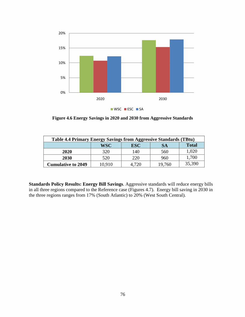
76
Figure 4.6 Energy Savings in 2020 and 2030 from Aggressive Standards
Standards Policy Results: Energy Bill Savings. Aggressive standards will reduce energy bills
in all three regions compared to the Reference case (Figures 4.7). Energy bill saving in 2030 in
the three regions ranges from 17% (South Atlantic) to 20% (West South Central).
0%
5%
10%
15%
20%
2020 2030
WSC ESC SA
Table 4.4 Primary Energy Savings from Aggressive Standards (TBtu)
WSC ESC SA Total
2020 320 140 560 1,020
2030 520 220 960 1,700
Cumulative to 2049 10,910 4,720 19,760 35,390

77
Figure 4.7 Energy Bill Savings from Aggressive Standards Policy
Standards Policy Results: Levelized Cost of Energy Efficiency. The levelized cost reflects the
cost to achieve a particular amount of energy saving through commercial energy efficiency
policies. Table 4.5 shows the levelized cost of electricity, natural gas and total energy efficiency
for the standards policy. Both the electricity and natural gas numbers are lower than the current
energy rates for commercial business in most southern states.
Table 4.5 Levelized Cost of Energy Efficiency from Standards Policy in 2020
Electricity Efficiency (¢//kWh) 3.1
Natural Gas Efficiency (¢/Therm) 3.1
Total Energy Efficiency ($/MMBtu) 9.3
Standards Policy Results: Economic Test. While energy bill savings measures commercial
benefits, the costs of implementing standards are both the private and public. Private parties
invest in the more expensive but higher efficient appliances while the public costs are those
associated with administrators incur administration and program.
These standards are being evaluated for 20 years starting in 2010 and the investments will occur
during the same period, the energy savings will continue beyond this period, for the lifetime of
the products installed through 2030. Figure 4.8 illustrates the costs ending in 2030, and extended
benefits from the aggressive standards policy. The energy bill savings exceed the public and
private investments by many times, indicating that the policy is highly cost-effective. An
“Annual Cost and Saving” table in Appendix D.4 summarizes the cost and saving from standards
policy as well as the HVAC retrofit policy and the commercial combined policy and it further
emphasizes the dynamic nature of cost and savings pattern and the cost-effectiveness of the
policy.
0%
5%
10%
15%
20%
25%
2010 2015 2020 2025 2030
WSC ESC SA

78
Figure 4.8 Costs and Savings from Aggressive Standard Policy
Table 4.6 shows the regional public and private cost in 2020 and 2030 and net present values
calculated for the Total Resource Test. The benefit-cost ratio is one measure of the cost
effectiveness of a program. A ratio greater than 1 indicates higher benefits than costs.
Table 4.6 Total Resource Test for Aggressive Standards Policy
(Million $2007)
B/C
Annual Public Costs Annual Private Costs Total
Costs
Total Savings
Administration
Cost
Investment
Cost
Investment and
Others*1
Cumulative
Costs
Cumulative
Savings *2
2020 10 0 2,170 16,050 31,730
4.6 2030 10 0 3,620 26,270 81,320
NPV 80 0 26,220 26,300 109,400 *
1 A range of investment related to “Office Equipment (PC)” “Office Equipments (Non PC)” and “Other” end uses
are estimated externally. Total resource test used the mid range value, which is considered as the best estimate. For
more details, please reference to Appendix D.3
*2 NPV of cumulative savings includes post 2030 savings
0
5
10
15
20
2010 2015 2020 2025 2030 2035 2040 2045 2050
Bill
ion
07
$
Energy Bill Savings Public Investment Private Investment Cost
79
4.3.2 Commercial Building HVAC Retrofit
Background. New, high efficiency energy efficient heating and cooling technologies can reduce
an energy bill up to 25% (Farrel et.al, 2007).To be effective, a commercial building HVAC
retrofit program should provide information and incentives for property owners to replace lower
efficiency HVAC systems with newer, more efficient ones.
Retrofitting in the South. Some southern states and utilities have begun to implement programs
that encourage commercial building HVAC system efficiency upgrades. States can use Energy
Efficiency Resource Standards to motivate utilities to work with energy services companies to
upgrade performance of commercial building systems (Amann et al., 2005). These energy
services companies, also known as ESCO‟s, can offer contracting services with financing options
based on the payback period for the energy savings realized. Utilities may facilitate this process
by offering incentives tied to reduction in energy demand.
States also can play an important role in encouraging energy efficiency by mandating minimum
efficiency requirements in public buildings. According to the U.S. Environmental Protection
Agency, several southern states, such as Alabama, Florida, North Carolina, and Virginia have
policies that promote energy efficiency in public buildings (EPA, 2008). South Carolina requires
that new and renovated public buildings attain LEED Silver certification, or the equivalent. The
U.S. Green Building Council states that many local governments across the region require
energy and green building certifications for public buildings (U.S. Green Building Council,
2009). States may choose to work closely with utilities and local governments to more
effectively use available federal funding. Financial support could be in the form of efficiency
grants, low interest loans, tax credits, or rebates. Providing flexible and widely available
financial incentives can go a long way toward stimulating investment in high efficiency
commercial building upgrades (World Resources Institute, 2009).
Commercial Building HVAC Retrofit Policy. The retrofit policy conceptualized in this study
could be made up of a set of teams whose task is to evaluate commercial building space within
their home state or region. These teams would distribute information about energy efficiency and
the eligibility requirements for available financial incentives. Each team would also provide
auditing services which identify potential energy savings achievable through individual
technology or whole building system retrofits. Oversight of these teams would be managed by a
program administrator.
SNUG-NEMS Modeling. The policy as modeled in this study reduces the capital costs for
installation of nine higher efficiency technologies, each of which come from one of three end
uses: space heating, space cooling and ventilation. Seven technologies are incentivized by 30%.
A different incentive is applied to ventilation. The two ventilation technologies receive 9%
incentive.18 Appendix D.2 summarizes the incentivized technologies.
HVAC Retrofit Policy Results: Energy Efficiency. Primary energy consumption is reduced as
a result of this policy (Figure 4.9). The total reduction of primary energy in 2030 is 316 TBtu.
18
Ventilation has a lower incentive rate because the relative costs are closer among technology vintage classes and a
larger incentive seemed to be more costly than necessary.
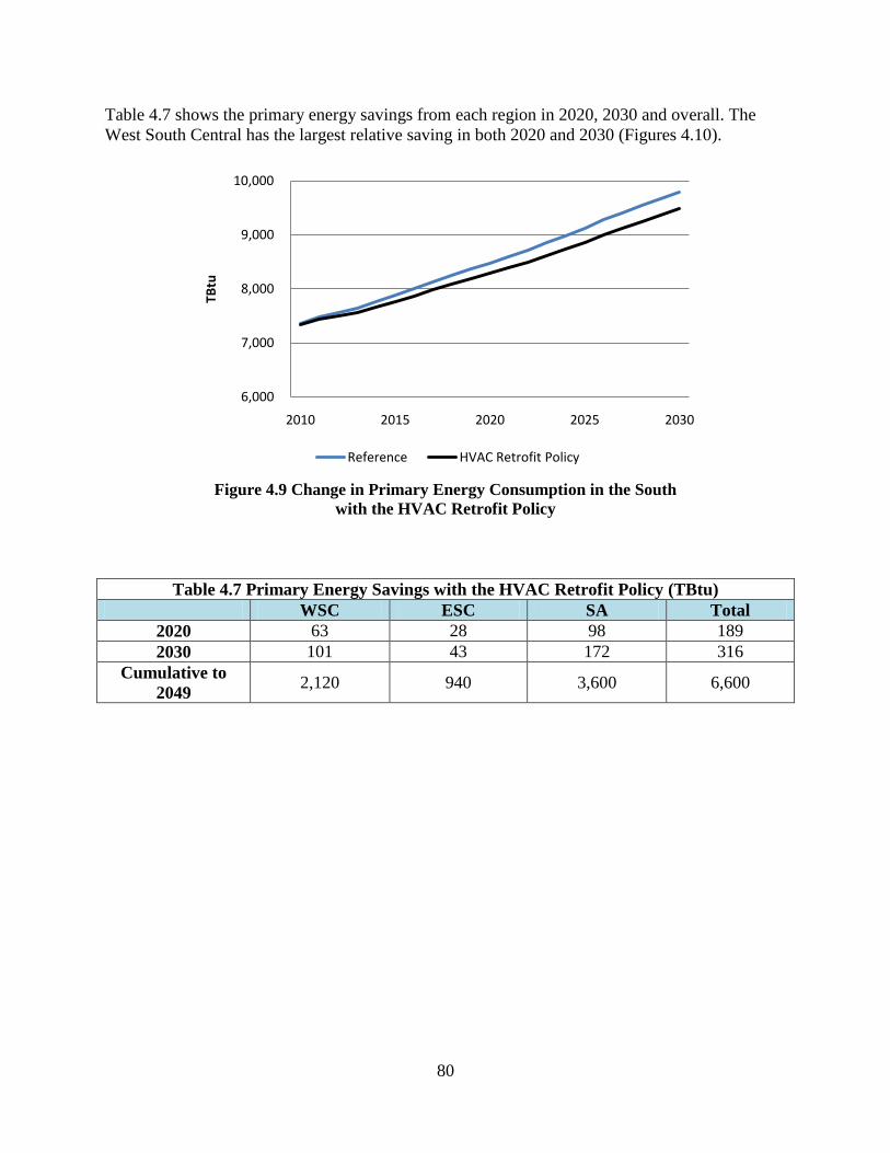
80
Table 4.7 shows the primary energy savings from each region in 2020, 2030 and overall. The
West South Central has the largest relative saving in both 2020 and 2030 (Figures 4.10).
Figure 4.9 Change in Primary Energy Consumption in the South
with the HVAC Retrofit Policy
Table 4.7 Primary Energy Savings with the HVAC Retrofit Policy (TBtu)
WSC ESC SA Total
2020 63 28 98 189
2030 101 43 172 316
Cumulative to
2049 2,120 940 3,600 6,600
6,000
7,000
8,000
9,000
10,000
2010 2015 2020 2025 2030
TBtu
Reference HVAC Retrofit Policy

81
Figure 4.10 Primary Energy Savings in 2020 and 2030 with the HVAC Retrofit Policy
HVAC Retrofit Policy Results: Energy Bill. The commercial HVAC retrofit program modeled
in this study achieves a reduction in commercial energy bill of 2 to 3% by the year 2020 (Figure
4.11). The WSC‟s energy bill saving is noticeably higher than the other regions after 2020.
Figure 4.11 Energy Bill Savings from the HVAC Retrofit Policy
0%
1%
2%
3%
4%
2020 2030
Pe
rce
nta
ge R
ed
uct
ion
WSC ESC SA
0%
1%
2%
3%
4%
5%
6%
2010 2015 2020 2025 2030
Pe
rce
nta
ge R
ed
uct
ion
WC ESC SA

82
HVAC Retrofit Policy Results: Levelized Cost. The natural gas efficiency improvement
modeled for this policy is smaller than 1% of the total energy efficiency from the same policy.
Therefore, only the levelized cost of electricity efficiency and total energy efficiency are
estimated. Compared with the standards policy, the HVAC retrofit policy is higher in cost (Table
4.8). However, the levelized cost of electricity is still lower than most of the commercial
electricity rates in the southern States.
Table 4.8 Levelized Cost of Energy Efficiency from the HVAC Retrofit Policy
in 2020
Electricity Efficiency(¢//kWh) 4.2
Total Energy Efficiency ($/MMBtu) 12.3
Economic Tests. The private investment cost to carry out the HVAC retrofit policy is negative
meaning business‟s pay less for the equipment that is incentivized than they would have paid for
less efficient equipment without incentives. Note that this negative cost is offset by the cost of
the subsidy, shown as public investment (Figure 4.12). Energy bill savings exceeds the costs of
this program by almost 150%, which indicates the cost-effectiveness of the HVAC retrofit policy
(Table 4.9). The annual savings and costs are shown in Appendix D.4.
Figure 4.12 Costs and Savings from HVAC Retrofit Policy
-1
0
1
2
3
4
2010 2015 2020 2025 2030 2035 2040 2045 2050
Bill
ion
07
$
Energy Bill Saving Public Investment Private Investment Cost

83
Table 4.9 Total Resource Test for HVAC Retrofit Policy
(Million $2007)
B/C
Annual Public Costs Annual Private
Costs
Total
Costs
Total
Savings
Administration
Cost
Investment
Cost
Investment and
Others
Cumulative
Costs
Cumulative
Savings
2020 50 1,580 -540 4,550 6,390
2.4 2030 50 1,760 -620 8,540 14,000
NPV 570 11,050 -3,070 8,540 20,850
4.4 COMBINED COMMERCIAL POLICIES, RESULTS
The rest of this chapter describes the analysis of combining the aggressive standards and HVAC
retrofit policies. SNUG-NEMS modeling effects can be overlapping and synergistic so results
will not add up to the sum of the previous results.
4.4.1 Energy Efficiency
By implementing the combined commercial policies, the annual energy efficiency gain in 2030
in the South is 1,980 trillion Btu in the reference scenario. This represents a 20% reduction in
energy consumption compared to the reference case. (Figure 4.13) The dotted lines on this plot
represent a sensitivity analysis for these policies. The sensitivity analysis was done to determine
whether modeling a generic carbon constraint, called the Carbon Constrained Future (CCF)19
,
would dramatically reduce or increase the effectiveness of these particular policies.
Figure 4.13 Primary Energy Consumption in South U.S. with Commercial Policies
19
CFF is explained in detail in section 6.3.2
6,000
7,000
8,000
9,000
10,000
2010 2015 2020 2025 2030
Trill
ion
Btu
Reference Commercial EE Policies Only
Carbon Constrained Future (CCF) CCF+Commercial EE Policies
20%
14%

84
The percentage energy saving from the combined policies is very similar to that from aggressive
standards alone because 83% of the total commercial energy savings come from the standard
policy. The West South Central region shows the largest relative saving of 14% in 2020 and 21%
in 2030 (Figure 4.14). In terms of actual Btu avoided, the South Atlantic has the greatest savings
in both 2020 and 2030, as it is shown in Table 4.10.
Figure 4.14 Energy Efficiency Potential in 2020 and 2030 with Commercial Policies
0%
5%
10%
15%
20%
25%
2020 2030
Pe
rce
nta
ge R
ed
uct
ion
WSC ESC SA
14% 14%
12%
20%
18%
21%

85
4.4.2 Energy Bill Savings
Commercial savings due to energy efficiency policies in all three regions exceed ten percent in
2020 and reach approximately 20% in 2030 (Table 4.11). Under the reference scenario,
commercial consumers would pay an estimated $11 billion less in energy bills in 2020 and $21
billion less in 2030. Figure 4.16 shows how bill savings change over time.
Table 4.11 Energy Bill Savings (Billion 07$)
2020 2030
WSC $3.5 16% $7.0 24%
ESC $1.3 12% $2.5 20%
SA $6.1 14% $11.7 22%
South Total $10.9 15% $21.2 22%
Figure 4.16 Energy Bill Savings from Commercial Policies – Reference Scenario
0%
5%
10%
15%
20%
25%
2010 2015 2020 2025 2030
Pe
rce
nta
ge R
ed
uct
ion
WSC ESC SA
Table 4.10 Primary Energy Savings from Commercial Policies (TBtu)
WSC ESC SA
2020 360 150 620
2030 600 260 1,120
Cumulative to 2049 12,500 5,440 22,830

86
4.4.3 Economic Test of Combined Commercial Policies
According to the total resource test, these commercial sector policies are cost-effective (Table
4.12). Private investment on commercial energy efficiency measures drops by over 50% in 2020
while public investment is doubled in the same year (Figure 4.17). This is because most of the
retrofitting starts in 2020 and the associated subsidies drive the changes in public and private
investment after that year. Private investment is increasing over time related to office equipment
and other end use purchases.
Table 4.12 Total Resource Test for Commercial Policies
(Million $2007)
B/C Annual Public Costs
Annual
Private Costs
Total
Costs
Total
Savings
Administration
Cost
Investment
Cost
Investment
& Other
Cumulative
Costs
Cumulative
Savings
2020 60 2,050 890 23,590 59,500
4.0 2030 60 2,350 2,180 31,530 94,100
NPV 680 15,230 15,660 31,530 126,300
Figure 4.17 Costs and Savings from Commercial Policies-Reference Scenario
4.5 SUMMARY AND DISCUSSION OF RESULTS FOR COMMERCIAL SECTOR
The commercial energy efficiency policy bundle is forecasted to help the South achieve a 14%
primary energy reduction in 2020 (1,200 TBtu saving from EIA‟s reference forecast) and a 20%
reduction in 2030 (2,100 TBtu saving compared to EIA‟s projection). Aggressive standards,
individually, could reduce the South‟s primary energy consumption by almost 18% in 2030
0
5
10
15
20
25
2010 2015 2020 2025 2030 2035 2040 2045 2050
Bill
ion
07
$
Energy Bill Saving Public Investment Private Investment

87
while commercial HVAC retrofit policy would reduce by nearly 3%, in 2030, relative to the
reference scenario. Figure 4.18 shows most of the energy efficiency savings in commercial
sector is from standards policy while HVAC retrofit policy is also significant. The levelized
costs of electricity and natural gas efficiency are low for both commercial policies, compared to
the energy rates that are currently charged in the South. Table 4.14 summarizes the energy
savings potential by policy that has been discussed in this chapter.
Figure 4.18 Commercial Energy Savings by Policy in 2030
Table 4.14 Commercial Primary Energy Savings
- Reference Scenario (Trillion Btu)
2020 2030
WSC ESC SA Total WSC ESC SA Total
Aggressive Equipment
Standards 360 150 630 1,140 560 250 1,050 1,860
HAVC Retrofit 100 40 160 300 130 50 200 380
Policy Bundle 370 160 650 1,180 630 280 1,170 2,080
These policies could generate over $20 billion in energy bill saving in 2030. While there are
costs to public and private entities, these costs are relatively small compared to the benefits. Both
policies are cost-effective as measured by the total resource test.
Standards Policy
1,852 TBtu,
83%
Retrofit Policy
380 TBtu,
17%

88
4.5.1 Comparison with Other Studies
A large number of studies have examined topics related to the energy efficiency potential in the
South and the key results from some of them are summarized in Figure 4.19. In a recent review,
Brown and Chandler (2009) examined 26 energy efficiency potential studies published over the
past 12 years. They conclude that the energy efficiency potential for the South‟s commercial
sector in 2020 is 1,400 TBtu which equals 14% of the region‟s commercial energy consumption
forecast. Brown and Chandler‟s result is very close to the estimates from this study (14% and
1,200 TBtu in 2020). Another study, Brown et al. (2009), covering the Appalachian region
showed somewhat a larger energy efficiency potential from the commercial sector. They
estimated that the Appalachian region, which includes many of the Southern states, could
achieve 22% savings from energy efficiency in the commercial sector in 2020. The discrepancy
between this study and the Appalachia study may be attributed to the different policy coverage.
In this study, the estimated commercial energy savings come from the policy bundle which
includes only two policies, commercial appliance standards policy and HVAC retrofit policy.
However, the Appalachia study also included building codes and commissioning of the existing
building as part of their commercial policy package and the energy savings associated with these
two polices are significant.
In the same year, McKinsey and Company (2009) released their estimates of national energy
efficiency potential based on their “NPV-positive potential for energy efficiency” approach. This
report includes results for each individual sector. McKinsey‟s commercial energy efficiency
potential for the South is 32% in 2020, which means 3,000 TBtu of energy consumption could be
avoided in a cost effective way. This estimate is more than twice as high as our result for at least
three reasons. First, beyond commercial buildings and office equipment, McKinsey identified the
potential from community infrastructure, such as water purification treatment, water distribution,
street and traffic lights, as 13% of the national total energy efficiency, and these savings are not
fully captured in our study. Second, McKinsey identified certain cost effective measures to
improve energy efficiency of buildings and office equipments that are not modeled in our study,
such as voluntary building standard for private commercial building and mandatory benchmarks
or standards for government buildings. Finally, the McKinsey study focuses on “economic
potential” and not “achievable potential”, which takes into account the inability of policies to
realize all of the cost-effective energy savings.

89
Figure 4.19 Comparison of Estimates of Commercial Energy Efficiency Potential in 2020
from Other Key Studies
In summary, our estimate falls in the middle of the range, it is higher than the Interlaboratary
Working Group‟s (IWG) Moderate scenario estimate of 9.4% (equivalent to 1,700 TBtu avoided
consumption) while lower than IWG (2000) Advanced scenario estimate of 19.1% (3,400 TBtu
avoided consumption. Though the IWG analysis was a national level study, the gap between our
estimates and IWG‟s is not due to regional idiosyncrasies. Rather, as with the McKinsey and
Appalachia (2009) studies, a significant portion of the commercial sector energy efficiency
potential estimated in IWG (2000) Advanced is attributed to new buildings through a building
codes policy. As discussed in the next section, a commercial building codes policy was excluded
from this study.
EPRI (2009) offers an estimate of commercial electricity efficiency from the utility point of
view.20
In 2020, the commercial sector realistic potential is estimated by EPRI to be 5% and
maximum potential is 10%. They are both lower in comparison to our results. Because EPRI
only considers the electricity efficiency potential that can be realized through utilities‟ programs,
appliance standards as well as other approaches that are implemented by state and federal
government regulations are not considered. This means that EPRI‟s electricity efficiency
potential estimate covers only a portion of the overall commercial sector potential that other
studies estimate.
4.5.2 Limitations and Needs for Future Research
This analysis of the energy efficiency potential in the South uses an integrated energy model
(SNUG-NEMS) with many strengths and advantages over alternative approaches. However, the
analysis could be strengthened in several ways.
20
The EPRI estimate is not shown in Figure 4.19 because they estimate electricity not total energy efficiency
potential.
0%
5%
10%
15%
20%
25%
30%
35%
Energy Efficiency in
the South (2010)
Chandler and Brown
(2009)
Brown et al. (2009)
IWG (2000) Moderate
IWG (2000) Advanced
McKinsey (2009)
90
A. Include more technology options in both policies to identify more energy efficiency
potential. The number of technologies modeled in this study is limited. There are 59
different types of technologies in the commercial technology input file. Thirty seven of
them were chosen to be subject to more stringent standards. In the HVAC retrofit policy,
nine types of technologies are incentivized. Being selective in choosing technology
subjects, we limited the number of technologies modeled, therefore underestimating the
energy efficiency potential, especially for the retrofit policy.
B. Account for real market behavioral shifting to identify a wider range of energy
efficiency potential. Due to the limitations in SNUG-NEMS, we assume there is no
shifting across classes of equipment due to our policies. For instance, even if the retrofit
incentives make the rooftop Air-Source Heat Pumps more economically desirable than a
Rooftop Air Conditioner for heating, consumers who have a Rooftop Air Conditioner
cannot switch to purchase a rooftop Air-Source Heat Pump. Instead, their purchase
decision is limited to alternatives within their existing technology class. In practice,
however, this is not true because consumers have freedom to choose between different
types of technologies in a free market. Accounting for behavior shifting that is currently
limited by SNUG-NEMS, could identify more energy efficiency potential.
C. Internalize the cost estimates. Most of our analysis is conducted inside the SNUG-
NEMS model so that we can fully capture the interplay between different factors. There
are only two exceptions. The administrative cost of the two policies and the private
investment costs associated with the office PCs, non-PC office equipment and other
equipment are estimated externally because SNUG-NEMS does not report these costs.
Appendix D.3 explains the method developed in this study to calculate the administrative
costs and investment costs associated with office equipments and miscellaneous end uses.
Future work that would refine this analysis includes internalizing the costs in SNUG-
NEMS modeling process.
D. Additional sensitivity analysis could add more nuance to the results. For example,
with more time, a wider range of standards, standards customized by end-use, or more
retrofit policies could have been evaluated. That would allow us to explore greater energy
potentials in the South‟s commercial sector. In addition, sensitivity analyses on fuel
prices and discount rates would offer a range of energy efficiency potential under
different future scenarios.
E. Certain benefits are beyond the scope of this report, but should be acknowledged.
The savings discussed here are primarily energy bill savings. However, in the real world,
energy efficiency could help achieve not only energy savings but also environmental and
public health benefits by reducing pollution such as CO2, SOx and NOx from being
emitted. These benefits may have significant value to society making the pursuit of
energy efficiency policies even more attractive. Public health and environmental benefits
are extremely hard to monetize but we would be remiss not to mention them.

91
F. Other policy options also have the potential to expand the energy efficiency
potential in the South. For example, new buildings were not a focus of our policies but
are a fertile area to pursue energy efficiency. New building codes were initially thought
of as likely to be cost effective, however, due to the difficulties in SNUG-NEMS
modeling, it was excluded from our analysis. In SNUG-NEMS, the relevant building
code input file considers only the wall and roof rather than a whole set of building
envelope which could also include windows and doors. In that case, a tighter building
code with new envelope standard in SNUG-NEMS leads to an increase in energy
consumption because the decrease in heating demand in the winter is offset by the
growing demand from cooling in the summer. As a result of this counterintuitive
outcome, we did not include building codes as part of our commercial energy efficiency
policy bundle. Therefore, our policies are primarily focused on the existing commercial
buildings though the appliance standard policy applies to both existing buildings and new
constructions.

92
5. ENERGY EFFICIENCY IN INDUSTRY
5.1 INTRODUCTION TO THE INDUSTRIAL SECTOR IN THE SOUTH
The industrial sector in the South consumed about 16,500 Trillion Btu (or 16.5 quad) of energy
in 2007 (EIA, 2009), which comprises 50% of the total U.S. industrial energy consumption.
According to the EIA‟s Annual Energy Outlook (AEO) 2009, industrial consumption will remain
significant, but shows a decreasing trend into the future. The reference forecast of industrial
energy consumption in the South region is illustrated in Figure 5.1. Two-thirds of the industrial
energy consumption is normally used for production processes, while one third of the energy is
consumed as feedstock in several industries, such as chemicals, petroleum refining, and plastics
manufacturing. Industrial energy consumption in the South is expected to remain relatively
consistent at around 14,000 Trillion Btu through 2030 (EIA, 2009).
Figure 5.1 Energy Consumption Reference Forecast for Industry in the South (EIA, 2009)
Industrial energy users consume a wide variety of energy sources and use them to produce steam,
heat, and electricity for operating equipment. Figure 5.2 illustrates the variety of fuels used by
southern industries. Electricity and its related losses account for 28 percent of usage, while liquid
fuels and natural gas respectively account for 36 and 24 percent.
0
2
4
6
8
10
12
14
16
18
20
1995 2000 2005 2010 2015 2020 2025 2030
En
erg
y C
on
sum
pti
on
(Q
ua
dri
llio
n B
tu)
Historical Projected
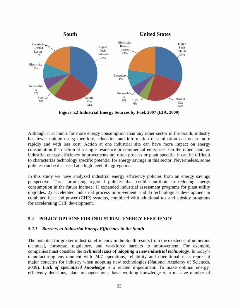
93
Figure 5.2 Industrial Energy Sources by Fuel, 2007 (EIA, 2009)
Although it accounts for more energy consumption than any other sector in the South, industry
has fewer unique users; therefore, education and information dissemination can occur more
rapidly and with less cost. Action at one industrial site can have more impact on energy
consumption than action at a single residence or commercial enterprise. On the other hand, as
industrial energy-efficiency improvements are often process or plant specific, it can be difficult
to characterize technology specific potential for energy savings in this sector. Nevertheless, some
policies can be discussed at a high level of aggregation.
In this study we have analyzed industrial energy efficiency policies from an energy savings
perspective. Three promising regional policies that could contribute to reducing energy
consumption in the future include: 1) expanded industrial assessment programs for plant utility
upgrades, 2) accelerated industrial process improvement, and 3) technological development in
combined heat and power (CHP) systems, combined with additional tax and subsidy programs
for accelerating CHP development.
5.2 POLICY OPTIONS FOR INDUSTRIAL ENERGY EFFICIENCY
5.2.1 Barriers to Industrial Energy Efficiency in the South
The potential for greater industrial efficiency in the South results from the existence of numerous
technical, corporate, regulatory, and workforce barriers to improvement. For example,
companies must consider the technical risks of adopting a new industrial technology. In today‟s
manufacturing environment with 24/7 operations, reliability and operational risks represent
major concerns for industry when adopting new technologies (National Academy of Sciences,
2009). Lack of specialized knowledge is a related impediment. To make optimal energy-
efficiency decisions, plant managers must have working knowledge of a massive number of
Liquid
Fuels
Subtotal36%
Natural
Gas
24%
Coal
5%
Renewable
s
7%
Electricity
9%
Electricity
Related
Losses19%
South
Liquid
Fuels
Subtotal30%
Natural
Gas
24%
Coal
6%
Renewable
s
6%
Electricity
11%
Electricity
Related
Losses23%
United States

94
technologies (McKinsey and Company, 2008). Researching new technologies consumes time
and resources, especially for small firms, and many industries prefer to expend human and
financial capital on other investment priorities (Worrell and Biermans, 2005).
Relatively high initial costs for industrial energy-efficiency improvements result in longer
payback periods than for traditional equipment. Senior managers often delay investing in costly
refurbishments because they are uncertain about the longevity of their companies (McKinsey and
Company, 2008, p. 9). Plant closures and production downturns in the textile industry in North
Carolina and Georgia and in aluminum manufacturing in Kentucky and Tennessee illustrate that
these are real concerns, particularly during the economic recession that began in 2008. Projects
to improve energy efficiency have to compete for resources against projects that achieve other
company goals and against familiar technologies. A large share of capital goes toward meeting
government standards for health, safety, security, and emissions; the remaining discretionary
capital is then allocated to other goals such as product improvement, production expansion, and
(finally) cost savings such as energy efficiency. This lack of access to capital is one of the most
significant barriers to energy efficiency improvements in industry (CCCSTI, 2009).
In the United States, existing fiscal policies are often unfavorable to investments in industrial
efficiency. The current federal tax code discourages capital investments in general, as opposed to
direct expensing of energy costs. Furthermore, outdated tax depreciation rules require firms to
depreciate energy efficiency investments over a longer period of time than many other
investments (Brown and Chandler, 2008). Existing regulations can also be unfavorable to
industrial energy efficiency. The threat of triggering a New Source Review has prevented many
upgrades from occurring (Brown and Chandler, 2008). Significant utility company
interconnection fees, overly layered permitting processes, and the lack of net-metering policies
provide disincentives for manufacturing plants to capture waste energy for the generation of
electricity in combined heat and power systems. For example, many states have low limits for
individual projects to receive net metering, such as 100 kW for commercial and industrial
projects in Georgia, 30 kW in Kentucky, and 25 kW in West Virginia (Figure 5.3). Finally,
policy uncertainty about the future cost of carbon emissions and the absence of an international
climate agreement are leading to competitiveness concerns and reduced cooperation across firms
(CCCSTI, 2009).

95
Figure 5.3 Geographic Variability of Net Metering (kW)
5.2.2 Policy Options
To address these barriers and support the expansion of industrial assessments in the South,
several programs have been investigated. Three complementary policies were chosen to be
modeled for energy efficiency potential. The first one is the Industrial Assessments of Plant
Utility Upgrades, with the expansion of Industrial Assessment Centers (IACs), oriented to small
and medium industrial sites, and increasing the scope of the Save Energy Now (SENA) program
for large firms. These two programs of the DOE are oriented to monitoring the principal
equipment that uses energy, such as motor and drive systems, pumps, steam systems, process
heating and fans. This equipment requires regular maintenance to ensure optimal performance.
The principal goal of these two programs is for specialists to visit the facilities and make
recommendations in order to guarantee the efficient use of energy in consumptive equipment and
identify replacements where needed. The second policy is to foster the acceleration of industrial
process improvements. This policy ensures the implementation of most efficient technologies.
The third policy option explored involves the stimulation of the installation of CHP units at
industrial sites.
Table 5.1 lists complementary actions to these three policies. The policies and programs listed
could be used as substitutions to the ones that were modeled in this study. The form of policies
adopted in different parts of the South will depend on which critical barriers and market failures

96
inhibit the market uptake of energy-efficient technologies and practices. These barriers vary
across industries and census divisions of the South. The specific choice of policies will also
reflect the goals and capacity of state and local agencies.
These three policies have the potential to reach nearly all southern industrial facilities by 2030.
Policy-makers would need to provide resources for advertising and information dissemination in
order to reach as many small to medium-sized industrial locations as possible. In addition,
program personnel may need to travel to sites for in-person visits to discuss the benefits of
industrial assessments. Once an industrial site requests an assessment, expert personnel should be
available to act. In order to increase the number of industrial assessments within the Region,
additional personnel should be added at current industrial assessment centers. The U.S.
Department of Energy could ask additional universities to form IACs to keep up with new
demand. This recommendation was taken into account in the last American Clean Energy
Leadership Act of 2009.
Table 5.1 Policy Actions that Support Industrial Energy Efficiency
Actions
Industrial Assessments
of Plant Utility
Upgrades
Policies to Accelerate
Industrial Process
Improvements
Industrial Combined Heat and
Power
Research, Development,
and Demonstration
Increased equipment and
system performance;
reduced installed cost
Increased equipment and
system performance;
reduced installed cost
Increased equipment and system
performance; reduced installed
cost
Financing Low or no interest loans
for capital improvements
Low or no interest loans
for capital improvements
Low or no-interest loans for
CHP equipment purchase
Financial Incentives
Assistance with energy
audit costs; grants and tax
credits
Grants and tax credits
Grants, tax credits, and
subsidies
- Extend the duration of existing
Investment Tax Credit (ITC)
- Subsidize a certain percentage
of initial installation costs
Pricing Time-of-use rates Time-of-use rates Reduced rates for natural gas for
CHP users
Voluntary Agreements N/A N/A N/A
Regulations Equipment standards Equipment standards Net metering and feed-in tariffs;
equipment standards
Information
Dissemination & Training
Campaigns to inform
small to medium-sized
industrial sites of
potential for energy and
cost savings
Training for on-site
personnel during first
Assessments to evaluate CHP
feasibility at site;
Campaign to inform industrial
sites of the potential for energy
and cost savings

97
Table 5.1 Policy Actions that Support Industrial Energy Efficiency
Actions
Industrial Assessments
of Plant Utility
Upgrades
Policies to Accelerate
Industrial Process
Improvements
Industrial Combined Heat and
Power
assessment;
Software tools to perform
Future assessments;
Campaign to inform large
industrial sites of the
potential for energy and
cost savings
Procurement
Assistance with
equipment procurement
to lessen lead times
Assistance with
equipment procurement to
lessen lead times
Assistance with equipment
procurement to lessen lead times
Market Reforms Public assistance fund Public assistance fund Public assistance fund
Planning Techniques
Outage management to
facilitate energy-
efficiency upgrades;
zoning and land use
planning
Outage management to
facilitate energy-
efficiency upgrades;
zoning and land use
planning
Outage management to facilitate
energy-efficiency upgrades;
zoning and land use planning
Capacity Building
Increase the number of
industrial assessment
universities and
personnel
Software development
Energy Service Company
(ESCO) Incubators
This table describes policy actions available that could further the savings from the policy packages modeled in this study.
The policy actions shown in italics are modeled in this study, while the others are not.
5.3 ENERGY EFFICIENCY POTENTIAL IN INDUSTRY IN THE SOUTH
This section describes the three policies evaluated to increase the industrial energy efficiency
saving. In order to capture the potential energy saving of each industrial group, the authors
collected a spreadsheet of state level data from the IAC and SENA programs which is presented
in the following section.
5.3.1 Spreadsheet Analysis for Industrial Assessments for Plant Utility Upgrades
This policy is designed to stimulate current growth in industrial assessments to improve the
plant‟s energy efficiency through the two DOE programs: IACs are oriented to save energy in
small and medium-sized firms and SENAs are designed for relatively larger energy consumers.
The information on energy use from these two programs had been analyzed below in order to
obtain the source of potential energy efficiency necessary to modify and run the unit energy
consumption in SNUG-NEMS.

98
Currently, there are 26 DOE Industrial Assessment Centers (IACs) located throughout the U.S.
(DOE/EERE, 2009k), with 13 located in the South. These centers are university-based, and
include teams comprised of both faculty and students who perform thorough energy analyses at
small to medium-sized industrial facilities within the local region. These assessments suggest
potential savings through improvements in energy efficiency, waste minimization, pollution
prevention, and productivity. Table E.1 in the appendix illustrates the activities of this program
in the South, including the number of assessments completed and the implementation rate of
recommendations.
In order to estimate the potential benefits of increasing IAC capacity, findings from recent
industrial assessments were evaluated. The resulting information was used with the state values
of shipment by industrial groups to determine potential energy savings. The details of this
spreadsheet analysis of IAC data are in Appendix E.1. The results of implementing increased
IAC capacity are shown in Tables 5.2 and 5.3. Details of the IAC modeling, including baseline
data, assumptions, and methodology are also detailed in Appendix E.1.
The IAC Program is estimated to reduce industrial energy consumption for small and medium
companies by: 0.2% in 2010, 1.0% in 2020, and 1.4% in 2030, with a total of 0.207 Quads of
savings in the South Region in 2030. The highest savings are expected to be in the West South
Central division, with 47% of the total savings, followed by the South Atlantic and East South
Central, with 31% and 22% respectively. Electricity constitutes a majority of the savings (0.129
Quads), while natural gas accounts for only 0.079 Quads of savings in 2030.
Table 5.2 Energy Savings from Increasing IAC Assessments and Training (TBtu),
Spreadsheet Analysis
Region
Electricity Savings Natural Gas Savings Total Energy Saved
2010 2020 2030 2010 2020 2030 2010 2020 2030
WSC 18 42 61 3 24 36 22 66 97
ESC 3 24 35 1 8 12 4 31 46
SA 3 22 33 3 21 31 6 44 64
Total 45 88 129 7 54 79 32 141 208
(Source: DOE, IAC and Team Analysis)
These savings figures assume that IAC assessments are able to increase to completing
assessments of nearly all small to medium-sized facilities by 2030 through an increase in the
workforce and the number of centers located in or near the region. In 2006, the South was home
to 14,112 small and medium manufacturing firms (50-250 employees). The energy savings could
increase to 1.4 percent of the projected sector use, which represents 0.207 Quads of savings. This
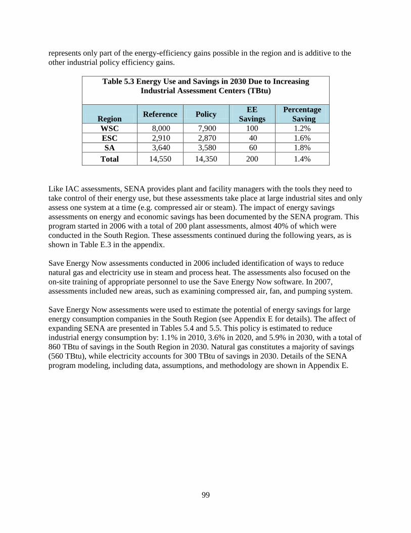
99
represents only part of the energy-efficiency gains possible in the region and is additive to the
other industrial policy efficiency gains.
Table 5.3 Energy Use and Savings in 2030 Due to Increasing
Industrial Assessment Centers (TBtu)
Region Reference Policy
EE
Savings
Percentage
Saving
WSC 8,000 7,900 100 1.2%
ESC 2,910 2,870 40 1.6%
SA 3,640 3,580 60 1.8%
Total 14,550 14,350 200 1.4%
Like IAC assessments, SENA provides plant and facility managers with the tools they need to
take control of their energy use, but these assessments take place at large industrial sites and only
assess one system at a time (e.g. compressed air or steam). The impact of energy savings
assessments on energy and economic savings has been documented by the SENA program. This
program started in 2006 with a total of 200 plant assessments, almost 40% of which were
conducted in the South Region. These assessments continued during the following years, as is
shown in Table E.3 in the appendix.
Save Energy Now assessments conducted in 2006 included identification of ways to reduce
natural gas and electricity use in steam and process heat. The assessments also focused on the
on-site training of appropriate personnel to use the Save Energy Now software. In 2007,
assessments included new areas, such as examining compressed air, fan, and pumping system.
Save Energy Now assessments were used to estimate the potential of energy savings for large
energy consumption companies in the South Region (see Appendix E for details). The affect of
expanding SENA are presented in Tables 5.4 and 5.5. This policy is estimated to reduce
industrial energy consumption by: 1.1% in 2010, 3.6% in 2020, and 5.9% in 2030, with a total of
860 TBtu of savings in the South Region in 2030. Natural gas constitutes a majority of savings
(560 TBtu), while electricity accounts for 300 TBtu of savings in 2030. Details of the SENA
program modeling, including data, assumptions, and methodology are shown in Appendix E.
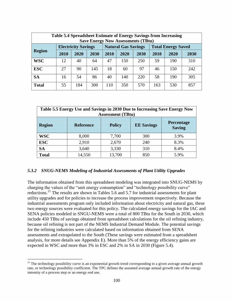
100
Table 5.4 Spreadsheet Estimate of Energy Savings from Increasing
Save Energy Now Assessments (TBtu)
Region Electricity Savings Natural Gas Savings Total Energy Saved
2010 2020 2030 2010 2020 2030 2010 2020 2030
WSC 12 40 64 47 150 250 59 190 310
ESC 27 90 145 18 60 97 46 150 242
SA 16 54 86 40 140 220 58 190 305
Total 55 184 300 110 350 570 163 530 857
Table 5.5 Energy Use and Savings in 2030 Due to Increasing Save Energy Now
Assessment (TBtu)
Region
Reference Policy EE Savings
Percentage
Saving
WSC 8,000 7,700 300 3.9%
ESC 2,910 2,670 240 8.3%
SA 3,640 3,330 310 8.4%
Total 14,550 13,700 850 5.9%
5.3.2 SNUG-NEMS Modeling of Industrial Assessments of Plant Utility Upgrades
The information obtained from this spreadsheet modeling was integrated into SNUG-NEMS by
charging the values of the “unit energy consumption” and “technology possibility curve”
reductions.21
The results are shown in Tables 5.6 and 5.7 for industrial assessments for plant
utility upgrades and for policies to increase the process improvement respectively. Because the
industrial assessments program only included information about electricity and natural gas, these
two energy sources were evaluated for this policy. The calculated energy savings for the IAC and
SENA policies modeled in SNGU-NEMS were a total of 800 TBtu for the South in 2030, which
include 450 TBtu of savings obtained from spreadsheet calculations for the oil refining industry,
because oil refining is not part of the NEMS Industrial Demand Module. The potential savings
for the refining industries were calculated based on information obtained from SENA
assessments and extrapolated to the South (These savings were estimated from a spreadsheet
analysis, for more details see Appendix E). More than 5% of the energy efficiency gains are
expected in WSC and more than 3% in ESC and 2% in SA in 2030 (Figure 5.4).
21
The technology possibility curve is an exponential growth trend corresponding to a given average annual growth
rate, or technology possibility coefficient. The TPC defines the assumed average annual growth rate of the energy
intensity of a process step or an energy end use.

101
Figure 5.4 Primary Energy Savings for Plant Utility Upgrade Policy
The greatest electricity and natural gas savings in 2030 would occur in the chemical industry,
although as a percentage reduction the values are not the highest because of the large energy
budgets of this industry in 2010. The largest percentages of reductions are in paper and cement.
4%
5%5%
3%
4%
2%
0%
1%
2%
3%
4%
5%
6%
2020 2030WSC ESC SA
Table 5.6 Total Energy Savings Industrial Assessment for
Plant Utility Upgrades (TBtu)
Year WSC ESC SA Total
2020 370 150 170 690
2030 430 170 200 800
Cumulative to 2050 10,500 4,400 5,000 19,900

102
Table 5.7 Results from the Industrial Assessment for Plant Utility Upgrades
in 2030 (TBtu)
Industrial
Sector
Electricity Savings Natural Gas Savings
Reference
Case
Policy
Case
%
Difference
Reference
Case
Policy
Case
%
Difference
Chemicals 167 166 -0.4% 337 290 -14%
Paper 76 60 -20.7% 92 85 -8%
Cement 20 18 -4.0% 10 9 -8%
Oil and gas
mining
91
81
-10.8%
226
165
-27%
Metal and
other non-
metal mining
39 35 -10.6% 14 10 -27%
Utility Upgrade Policy Results: Levelized Cost of Energy Efficiency. The levelized cost
reflects the cost to achieve a particular amount of energy saving through our industrial energy
efficiency policies. This study focuses on electricity efficiency potential, natural gas efficiency
potential and total energy efficiency potential from each individual policy.
Table 5.8 shows the levelized cost of electricity, natural gas and the total energy efficiency in the
Utility Upgrade policy. Both the electricity and natural gas numbers are lower than the energy
rates charged to industrial business in most of the southern states.
Table 5.8 Levelized Cost of Energy Efficiency from
Utility Upgrade Policy in 2020
Electricity Efficiency (¢//kWh) 0.9
Natural Gas Efficiency (¢/Therm) 15.7
Total Energy Efficiency ($/MMBtu) 1.1
Economic Tests. The costs and savings for this policy are shown in Table 5.9. Investment costs
are calculated from the cost information contained in the IAC and SENA programs. Both
programs present detailed information about costs required to update plant utilities for increasing
energy efficiency. All the investment costs are assumed to be made by the industry.
Nevertheless, policy-makers could consider a public subsidy as part of the investment scenario,
but that was not evaluated in this study. Administrative costs are assumed entirely by the public
sector, which represents less than one percent of the total costs. The government role is to
motivate industry to conduct energy efficiency assessments, through the creation of Champion
programs. Additionally the public sector could establish a program for the diffusion of best
practices in energy use for the 22 most significant industries, for small, medium and large firms
(for more details about the calculation see Appendix E section).

103
Table 5.9 Total Resource Test -- Industrial Assessment for
Plant Utility Upgrades Policy*
Year
(Million $2007)
B/C Public Costs Private Costs
Total
Discount
Costs
Total
Discount
Savings Annual
Administration
Cost
Annual
Investment Cost
Annual
(Investment & Other)
Cumulative
Costs
Cumulative
Savings
2020 10.6 0 750 8,600 17,100
2030 9.3 0 590 10,800 38,700
NPV 124 0 10,500 10,800 48,400 4.5
*Cumulative Costs beginning in 2010 and Savings beginning in 2011. NPV includes savings post 2030
Energy Bill Savings. This policy appears to be highly cost-effective. The energy bill savings
exceed the public and private investments by many times. This policy‟s energy savings are is
expected to decrease rapidly after 2030, since this is the last year when new assessments are
modeled.
Figure 5.5 Energy Bill Savings for Plant Utility Upgrade policy
5.3.3 Policies to Accelerate Industrial Process Improvements
Several studies have shown high energy savings potential in the highly energy-intensive
industries. A recent study of the National Academies (2009) recompiled these studies for 5
industries‟ potential energy savings in 2020: petroleum refining, iron and steel, cement,
chemicals manufacturing, and pulp and paper. These five industries represent 83% of the total
energy consumption in the South (EIA, 2006).
1
2
3
4
5
2010 2015 2020 2025 2030 2035 2040 2045 2050
Bil
lio
n 0
7$
Energy Bill Saving
Public Investment
Private Investment
104
The petroleum refining industry‟s energy savings are presented in 3 studies; the lowest estimate
of 0.3 quads, which represent 5% of energy consumption in 2020 came from McKinsey and
Company (2008). The highest estimate is a range of 1.68 to 3.94 quads published in a DOE
(2006j) report, with a range of 28-65% of reduction in consumption in 2020. The intermediate
range of saving, between 0.73 to 1.46 quads in 2020, was shown by the study of LBNL (2005),
with a range between 12 to 24%.
The iron and steel industry also presents an important opportunity for energy savings. McKinsey
and Company (2008) identified 0.3 quads or 22% of energy consumption in 2020. The AISI
study (2005) provided a higher level of energy savings at 0.79 quad, or 58% of energy use.
Three studies analyzed the cement industry, the lower estimation of energy savings is presented
by Brown M., et al (2001) with 0.08 or 19% quads of saving in 2020, followed by McKinsey and
Company with a 0.1 quads or 23%. The highest potential of savings is presented in the study of
Worrell (2004), with 0.29 quads or 67% of energy saving in 2020.
The chemical manufacturing industry was analyzed by three studies: the lowest level of savings
is presented in the NREL (2002) report with only 0.19 quads or 3.1% of energy use in 2020. A
similar result was presented in McKinsey with a potential for savings of 0.3 quads or 5% in
2020. The highest amount of savings was shown by Energetics Incorporated (US DOE 2007),
with a total of 1.1 quads or 18% of energy use in 2020.
Finally, the pulp and paper industry also represents a potential of energy savings through its
process improvement, from 0.14 quads or 6.1% in the CEF study to 0.85 quads or 37% of energy
use, in the study of Jacobs and IPST (2006).
Among the most prominent industrial process improvement technologies are super boilers, which
present over 95 percent fuel-to-steam efficiency (Industrial Technology Program (ITP) DOE,
2008). This technology is able to improve heat transfer thanks to the use of advanced firetubes
with extended surfaces that help achieve a compact design, reducing size, weight, and footprint.
The advanced heat recovery system combines compact economizers, a humidifying air heater,
and a patented transport membrane condenser. Many boilers used today are more than 40 years
old, suggesting a large energy-savings opportunity (Gemmer, 2007). This technology provides
compelling economic benefits to accelerate replacement of aging boilers (see Figure 5.6)

105
Figure 5.6 Gas-fired Super Boiler (Source: ITP 2008)
Table 5.10 lists each industry and business-as-usual (Reference) projected energy use. The
different estimates for energy-efficiency potential savings is shown by the two rightmost
columns.
Table 5.10 Estimated Energy Savings Due to Energy-Efficiency From
Accelerated Industrial Process Improvements (in TBtu)
Industry
Energy Use in the Reference
Case
Savings Over the Reference
Case
2009 2020 2030 2020* 2030**
Petroleum Refining 4,950 5,640 6,720
300
610 to 1,210
1,400 to 3,280
5,490
Iron & Steel 1,310 1,220 940 210 to 790 740
Cement 330 430 420 80
290 320
Chemicals
Manufacturing 5,540 5,280 4,490
300
190 to 1,100 1,150
Pulp & Paper 1,960 2,100 2,200 140 to 600
370 to 850 1,410
* Based on a review of studies for specific energy-using industries.
**Based on average of energy saving of 2020 savings projected to 2030

106
5.3.4 SNUG-NEMS Modeling to Accelerate Industrial Process Improvements
This policy as modeled in SNUG-NEMS resulted in a total savings of 1.38 quads in 2020 and
1.57 quads in 2030. This represents savings of 9% of energy in 2020 and 10% in 2030. The
highest energy efficiencies are in the West South Central region with 89% of the total savings
(see Table 5.11). Figure 5.7 shows energy efficiency gains by region, and WSC has the largest
potential.
Table 5.11 Primary Energy Savings Industrial Process Improvements (TBtu)
Year WSC ESC SA Total
2020 1,230 90 60 1,380
2030 1,350 150 70 1,570
Cumulative to 2050 36,000 3,180 1,840 41,100
Figure 5.7 Primary Energy Saving in the Industrial Process Improvement Policy
Table 5.12 shows the levelized cost of electricity, natural gas and the total energy efficiency
(including savings from liquid fuels with 344 TBtu in 2020) for this policy. Both the electricity
and natural gas numbers are lower than the energy rates charged to industrial business in most of
the southern states.
15%
17%
6%5%5%
2%
0%
2%
4%
6%
8%
10%
12%
14%
16%
18%
2020 2030WSC ESC SA

107
Table 5.12 Levelized Cost of Energy Efficiency from Process Improvement
Policy in 2020
Electricity Efficiency (¢//kWh) 2.4
Natural Gas Efficiency (¢/Therm) 23.8
Total Energy Efficiency ($/MMBtu) 3.6
Economic Tests. The costs and savings for the industrial policy to increase the process
improvement are shown in Table 5.13. The investment costs are calculated based an estimation
of the costs previously presented for the Plant Utility Upgrade policy. Considering that the
adoption of new technologies to improve energy efficiency is more costly, this study assumed
that the Plant Utility Upgrades policy represented 40% of the total investment cost of the Policy
to accelerate industrial process improvements. All the investment costs are assumed to be made
by the private-sector industry. Nevertheless, policy-makers could consider a public subsidy as
part of the investment scenario, but that was not evaluated in this study. Administrative costs are
assumed entirely by the public sector, which represents less than one percent of the total costs. It
is designed to motivate the industry to conduct process improvement, through the acquisition of
newest technologies. (See more details about the calculations in Appendix E section)
Table 5.13 Total Resource Cost Test for Process Improvement Policy
Year
(Million $2007)
B/C Public Costs Private Costs
Total
Discount
Costs
Total
Discount
Savings Annual
Administration
Cost
Annual
Investment Cost
Annual
(Investment & Other)
Cumulative
Costs
Cumulative
Savings
2020 6.5 0 1,700 20,000 57,300 -
2030 10.6 0 1,400 36,000 108,700 -
NPV 65.4 0 24,800 36,000 128,800 3.6
*Cumulative Costs beginning in 2010 and Savings beginning in 2011. NPV included savings post 2030
Energy Bill Savings. The Process Improvement Policy appears to be cost-effective. The energy
bill savings exceed the public and private investments by many times (see Figure 5.8). Energy
savings is expected to rapidly decrease returns after 2030.
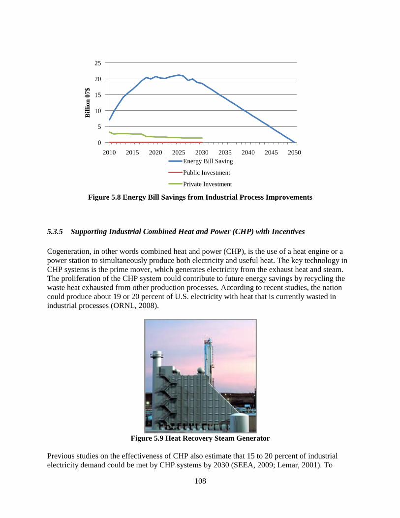
108
Figure 5.8 Energy Bill Savings from Industrial Process Improvements
5.3.5 Supporting Industrial Combined Heat and Power (CHP) with Incentives
Cogeneration, in other words combined heat and power (CHP), is the use of a heat engine or a
power station to simultaneously produce both electricity and useful heat. The key technology in
CHP systems is the prime mover, which generates electricity from the exhaust heat and steam.
The proliferation of the CHP system could contribute to future energy savings by recycling the
waste heat exhausted from other production processes. According to recent studies, the nation
could produce about 19 or 20 percent of U.S. electricity with heat that is currently wasted in
industrial processes (ORNL, 2008).
Figure 5.9 Heat Recovery Steam Generator
Previous studies on the effectiveness of CHP also estimate that 15 to 20 percent of industrial
electricity demand could be met by CHP systems by 2030 (SEEA, 2009; Lemar, 2001). To
0
5
10
15
20
25
2010 2015 2020 2025 2030 2035 2040 2045 2050
Bil
lio
n 0
7$
Energy Bill Saving
Public Investment
Private Investment
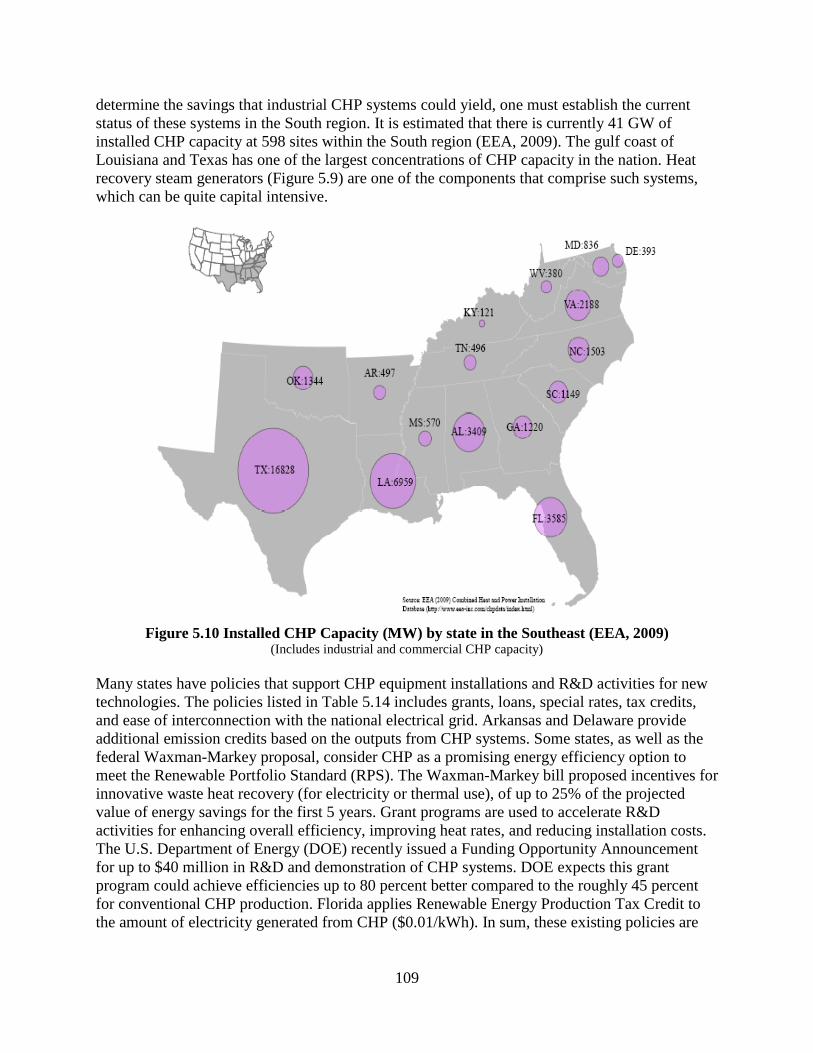
109
determine the savings that industrial CHP systems could yield, one must establish the current
status of these systems in the South region. It is estimated that there is currently 41 GW of
installed CHP capacity at 598 sites within the South region (EEA, 2009). The gulf coast of
Louisiana and Texas has one of the largest concentrations of CHP capacity in the nation. Heat
recovery steam generators (Figure 5.9) are one of the components that comprise such systems,
which can be quite capital intensive.
Figure 5.10 Installed CHP Capacity (MW) by state in the Southeast (EEA, 2009)
(Includes industrial and commercial CHP capacity)
Many states have policies that support CHP equipment installations and R&D activities for new
technologies. The policies listed in Table 5.14 includes grants, loans, special rates, tax credits,
and ease of interconnection with the national electrical grid. Arkansas and Delaware provide
additional emission credits based on the outputs from CHP systems. Some states, as well as the
federal Waxman-Markey proposal, consider CHP as a promising energy efficiency option to
meet the Renewable Portfolio Standard (RPS). The Waxman-Markey bill proposed incentives for
innovative waste heat recovery (for electricity or thermal use), of up to 25% of the projected
value of energy savings for the first 5 years. Grant programs are used to accelerate R&D
activities for enhancing overall efficiency, improving heat rates, and reducing installation costs.
The U.S. Department of Energy (DOE) recently issued a Funding Opportunity Announcement
for up to $40 million in R&D and demonstration of CHP systems. DOE expects this grant
program could achieve efficiencies up to 80 percent better compared to the roughly 45 percent
for conventional CHP production. Florida applies Renewable Energy Production Tax Credit to
the amount of electricity generated from CHP ($0.01/kWh). In sum, these existing policies are

110
designed to motivate plant owners to install new CHP systems and actively use their existing
equipment.
Table 5.14 Summary of CHP-Supportive Policies in the South
Type of Policy State Applicability and
Amount
Requirements and
Limits
Environmental
Regulations
AR, DE
Output-Based
Regulations,
Combined heat and
power (CHP)
systems can receive
emissions credits
Renewable Portfolio
Standard DC, MD, VA, WV
Grants for New
Technologies
EPA small business
innovation research
program (phase I
R&D funding by
$70,000, phase II
$225,000)
Interconnection
DC, TX, MW, KS,
FL, DE
DC, TX
Interconnection
Standards, up to 10
MW, KS (5MW), FL
(2MW) and DE
(1MW)
Long-term Loans for
Customer-side Distributed
Generation
$150 million
available
Renewable Energy
Production Tax
Credit FL
$0.01/kWh of
electricity produced
and sold
Renewable Energy
Tax Credit NC
35 % of the cost of
renewable energy
systems built
purchased, or leased
Loan
MS
Energy Investment
Program, interest rate
3%, max 7 years
$15,000 to $300,000

111
5.3.6 SNUG-NEMS Modeling of Industrial CHP with Incentives
To motivate plant owners to install more CHP equipment, policy makers must address several
technology barriers. Two key parameters that influence economic viability are operating costs
(driven by efficiency and fuel price) and capital costs (driven by initial installation costs)
(ORNL, 2008). We have developed a policy scenario to address the two factors. To assess the
magnitude of cost-effectiveness and achievable energy-efficiency improvements from CHP
proliferation, we have assumed adoption of a set of transformative energy policies: 1) extension
of the duration of existing tax credit programs and 2) acceleration of R&D activities.
The first part of the policy bundle was modeled in SNUG-NEMS by extending the duration of
the current Investment Tax Credits (ITC) included in the Energy Improvement and Extension
Act of 2008. Congress passed this law on October 3, 2008 and established a new ITC for CHP
systems. The credits began in 2008 and are currently scheduled to continue through 2016. In this
study, we assumed that policymakers would extend the duration of the ITC through 2030. In
addition, we implemented a 20% subsidy policy for accelerating additional installation of CHP
equipment. On balance, 30% of the total investment cost for new CHP systems would be
supported by government.
We also modeled grant programs that support R&D activities for improving the performance of
CHP systems. We assumed that the programs could increase the overall efficiency by 0.7%
annually and raise the average efficiency level up to 83% by 2030 without any additional
increase in installation cost. Table 5.15 shows that the overall efficiency values for the EIA‟s
reference case and those for our study. We approximated that the grant program would spend
$20 million annually to cost share the R&D of research entities. CHP system performance and
cost information from EIA were used to quantify energy savings and financial costs.
Table 5.15 Overall Efficiency by CHP System (Size)
Reference* Policy**
System Size
(kilowatts)
2020 2030 2020 2030
1 Engine 1,000 0.73 0.74 0.77 0.82
2 Engine 3,000 0.74 0.75 0.77 0.83
3 Gas Turbine 3,000 0.70 0.71 0.75 0.80
4 Gas Turbine 5,000 0.72 0.72 0.76 0.82
5 Gas Turbine 10,000 0.71 0.72 0.76 0.82
6 Gas Turbine 25,000 0.72 0.73 0.77 0.82
7 Gas Turbine 40,000 0.73 0.73 0.78 0.83
8 Combined Cycle 100,000 0.72 0.73 0.76 0.81 * Industrial CHP Technology Performance Data used for EIA‟s AEO 2009 projections
** We increased the overall efficiency of each CHP system by 0.7% annually and raised the efficiency level up to 83% by 2030.
When the CHP policy is implemented, the electricity generation capacity would increase by
29.1% in the South, and the Region could produce 38.1 TWh of electricity and 122 TBtu of
useful steam additionally. In sum, the South could produce 147.9 TWh of electricity and 1.1
Quads of useful steam from both existing (i.e. installed before the policy implementation) and

112
newly installed CHP equipment in 2030 (Figure 5.11 and 5.12).
Figure 5.11 Electricity Generation Capacity in the Industrial Sector (*Only industrial CHP capacity counted)
Figure 5.12 Energy Consumption and Production in Industrial CHP Systems in the South in
2030
10,000
14,000
18,000
22,000
26,000
30,000
2010 2015 2020 2025 2030
MW
Policy Reference

113
The WSC shows the highest cumulative primary energy savings of 3,351 TBtu followed by the
SA with 1,478 TBtu and the ESC with 591 TBtu (Table 5.16).
Table 5.16 Primary Energy Savings from CHP Policy (TBtu)
Year WSC ESC SA Total
2020 68 12 30 110
2030 178 32 78 289
Cumulative to 2050 3,350 590 1,480 5,420
We could expect more than 2% of the energy efficiency gains in the WSC and the SA in 2030
(Figure 5.13).
Figure 5.13 Primary Energy Savings from CHP policy
The impact of the policy would increase gradually throughout the study horizon. The total
installed CHP equipment in the South could reduce the total industrial energy consumption by
3.5% in 2020 and 4.7% in 2030 (Table 5.17).
Table 5.17 Energy Production and Consumption in Total CHP systems
Year
Total
Electricity
Production
(TWh)
Total
Steam
Production
(TBtu)
Total Fuel
Consumption
(TBtu)
Net Primary
Fuel Saved
(TBtu)
% of Energy
Saved
2020 118 1,020 2,410 408 3.5%
2030 148 1,140 2,720 613 4.7%
0.8%
2.3%
0.4%
1.0%0.8%
2.2%
0.0%
0.5%
1.0%
1.5%
2.0%
2.5%
2020 2030
Per
cen
tag
e o
f R
edu
ctio
n
WSC ESC SA
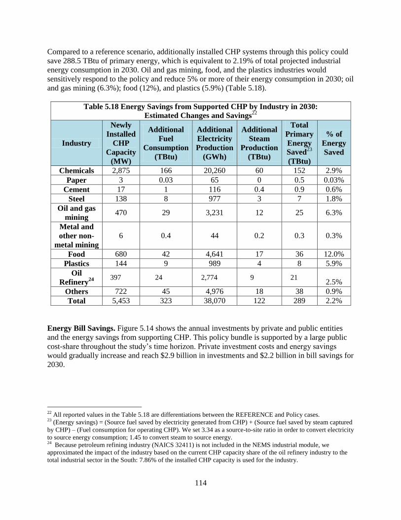
114
Compared to a reference scenario, additionally installed CHP systems through this policy could
save 288.5 TBtu of primary energy, which is equivalent to 2.19% of total projected industrial
energy consumption in 2030. Oil and gas mining, food, and the plastics industries would
sensitively respond to the policy and reduce 5% or more of their energy consumption in 2030; oil
and gas mining (6.3%); food (12%), and plastics (5.9%) (Table 5.18).
Table 5.18 Energy Savings from Supported CHP by Industry in 2030:
Estimated Changes and Savings22
Industry
Newly
Installed
CHP
Capacity
(MW)
Additional
Fuel
Consumption
(TBtu)
Additional
Electricity
Production
(GWh)
Additional
Steam
Production
(TBtu)
Total
Primary
Energy
Saved23
(TBtu)
% of
Energy
Saved
Chemicals 2,875 166 20,260 60 152 2.9%
Paper 3 0.03 65 0 0.5 0.03%
Cement 17 1 116 0.4 0.9 0.6%
Steel 138 8 977 3 7 1.8%
Oil and gas
mining 470 29 3,231 12 25 6.3%
Metal and
other non-
metal mining
6 0.4 44 0.2 0.3 0.3%
Food 680 42 4,641 17 36 12.0%
Plastics 144 9 989 4 8 5.9%
Oil
Refinery24
397 24 2,774 9 21
2.5%
Others 722 45 4,976 18 38 0.9%
Total 5,453 323 38,070 122 289 2.2%
Energy Bill Savings. Figure 5.14 shows the annual investments by private and public entities
and the energy savings from supporting CHP. This policy bundle is supported by a large public
cost-share throughout the study‟s time horizon. Private investment costs and energy savings
would gradually increase and reach $2.9 billion in investments and $2.2 billion in bill savings for
2030.
22
All reported values in the Table 5.18 are differentiations between the REFERENCE and Policy cases. 23
(Energy savings) = (Source fuel saved by electricity generated from CHP) + (Source fuel saved by steam captured
by CHP) – (Fuel consumption for operating CHP). We set 3.34 as a source-to-site ratio in order to convert electricity
to source energy consumption; 1.45 to convert steam to source energy. 24
Because petroleum refining industry (NAICS 32411) is not included in the NEMS industrial module, we
approximated the impact of the industry based on the current CHP capacity share of the oil refinery industry to the
total industrial sector in the South: 7.86% of the installed CHP capacity is used for the industry.

115
Figure 5.14 Energy Bill saving in Industrial CHP Policy
Economic Tests. Supporting CHP with incentives is cost-effective, with a benefit-to-cost ratio of
about 1.01 for participants. It is not, however, cost effective, with a ratio of 0.67 based on total
resource cost test. CHP systems are environmentally friendly equipment and they could
contribute to reducing CO2 emissions. The benefits expected from the CO2 emissions reduction
are not included in the benefit-cost ratio of this study. If we capture the environmental benefits
and include them in the calculation, the benefit-cost ratio would be 1.04, assuming that a ton of
CO2 increases in value from $15 to $51 over the study period.
Table 5.19 Total Resource Test for CHP Policy
(Million $2007)
B/C
Public Costs Private Costs Total
Discounted
Costs
Total
Discounted Savings
Annual
Administration
Cost
Annual Investment
Cost
Annual (Investment &
Other)
Cumulative
Costs Cumulative
Savings
2020 5 543 1,221 6,444 2,953
2030 5 1,276 2,932 16,930 7,826
NPV 56 5,214 11,660 16,930 11,380 0.67
(17,570**) (1.04**)
*Cumulative Costs beginning in 2010 and Savings beginning in 2011. NPV included savings post 2030
** In case that environmental benefits from CO2 emissions avoided by CHP systems are counted
0
500
1000
1500
2000
2500
3000
3500
2010 2015 2020 2025 2030 2035 2040 2045 2050
Mil
lio
n 0
7$
Energy Savings Public Investment Private Investment

116
5.4 COMBINED INDUSTRIAL ENERGY EFFICIENCY POLICIES
5.4.1 Energy Efficiency Results
The three combined industrial energy efficiency policies could reduce the total industrial energy
consumption by 15.8% under the no Carbon-Constrained Future (CCF) scenario and 16.5%
under a CCF in the South in 2030 (Figure 5.15).
Figure 5.15 Industrial Energy Consumption Projections
The three policies are significant contributors to energy efficiency gains. The West South Central
division presents the highest savings of 14% in 2020 and 21% in 2030, followed by the East
South Central with 10% in 2020 and 15% in 2030. The South Atlantic shows the lowest energy
savings levels, indicating only 7% in 2020 and 9% in 2030.
10
11
12
13
14
15
16
2010 2015 2020 2025 2030
Qu
ad
rill
ion
Btu
Reference
Carbon Constrained Future
Industrial EE policies
Industrial EE policies with Carbon-Constrained Future
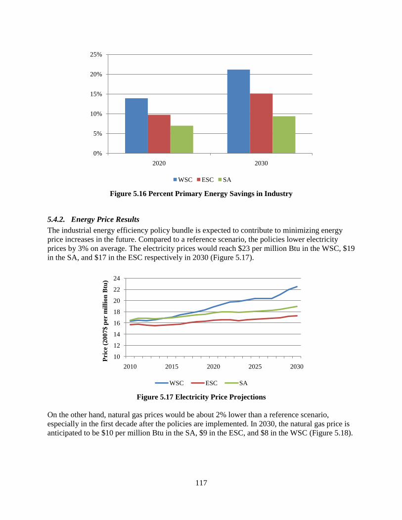
117
Figure 5.16 Percent Primary Energy Savings in Industry
5.4.2. Energy Price Results
The industrial energy efficiency policy bundle is expected to contribute to minimizing energy
price increases in the future. Compared to a reference scenario, the policies lower electricity
prices by 3% on average. The electricity prices would reach $23 per million Btu in the WSC, $19
in the SA, and $17 in the ESC respectively in 2030 (Figure 5.17).
Figure 5.17 Electricity Price Projections
On the other hand, natural gas prices would be about 2% lower than a reference scenario,
especially in the first decade after the policies are implemented. In 2030, the natural gas price is
anticipated to be $10 per million Btu in the SA, $9 in the ESC, and $8 in the WSC (Figure 5.18).
0%
5%
10%
15%
20%
25%
2020 2030
WSC ESC SA
10
12
14
16
18
20
22
24
2010 2015 2020 2025 2030
Pri
ce (
20
07
$ p
er m
illi
on
Btu
)
WSC ESC SA

118
Figure 5.18 Natural Gas Price Projections
5.4.3 Energy Bill Savings
The three industrial energy efficiency policies would increase energy bill savings in all three
census divisions (Figure 5.19). The savings are much greater in the West South Central states
than those in other census divisions. The percentage of reduction of the WSC starts at 7% in
2010, reaches a peak in 2017, remains constant until 2027, and then shows a slight drop in 2030.
The East South Central and South Atlantic show gradual increases in bill savings.
Figure 5.19 Percentage Change in Energy Bill Savings
0
2
4
6
8
10
12
2010 2015 2020 2025 2030
Pri
ce (
20
07
$ p
er m
illi
on
Btu
)
WSC ESC SA
0%
2%
4%
6%
8%
10%
12%
14%
2010 2015 2020 2025 2030
Per
cen
tag
e o
f R
edu
ctio
n
WSC ESC SA

119
5.5 SUMMARY OF RESULTS FOR INDUSTRIAL ENERGY EFFICIENCY
Our analysis of industrial energy efficiency policies suggests that the South could expect 11% of
energy efficiency gains in 2020 and 16% in 2030 by implementing the three policy bundles.
Since the South accounts for 50% of the total U.S. industrial energy use, these savings represent
a significant reduction in national energy consumption. Accelerating process improvements
could produce the greatest energy savings among the three policies, generating a 11% reduction
in industrial energy consumption in 2030. Expanding assessments of plant utility upgrades and
supporting CHP with incentives also reduce the energy required in this sector by 6% and 2%
respectively.
Figure 5.20 Industrial Energy Savings by Policy Package in 2030
The South could save 2.1 quads of industrial energy in 2030. The West South Central could
expect the greatest energy efficiency gains among the three census divisions in South, followed
by the South Atlantic and the East South Central (Table 5.20). These estimated savings are
similar to other efficiency studies. They demonstrate that significant gains can be achieved by
implementing industrial energy efficiency policies in the South.
Table 5.20 Summary of Industrial Primary Energy Savings
by Policy and Census Division in 2020 and 2030 (TBtu)*
Policy Year WSC ESC SA Total
Plant Utility Upgrades
2020 370 150 170 690
2030 430 170 200 800
Process Improvements
2020 1,230 90 60 1,380
2030 1,350 150 70 1,570
CHP 2020 70 10 30 110
2030 180 30 80 290
Combined Policy Bundle 2020 1,040 250 290 1,580
2030 1,380 370 400 2,150
* These results include the energy savings from Oil Refining Industry which was modeled in SNUG-NEMS.
Assessments
of Plant
Utility
Upgrades
801 TBtu
(30%)Process
Improvements
1,564 TBtu
(59%)
CHP with
Incentives
289 TBtu
(11%)

120
The first two policies for Plant Utility Upgrades and Process Improvements are cost effective
with a ratio of 4.5 and 3.6 respectively. On the other hand, supporting CHP with incentives is
cost ineffective when we consider only primary energy savings as benefits. However, the
benefit-cost ratio would be 1.04 if we capture benefits from avoided CO2 emissions by newly
installed CHP systems.
Table 5.21 Summary of Economic Tests by Policy (Million $2007)
Policy NPV
Cost NPV
Benefit B/C
Ratio
Cumulative
Savings to
2050 (TBtu)
Savings in 2030 (TBtu)
Plant Utility Upgrades 10,800 48,400 4.5 16,900 800
Process Improvements 36,000 129,000 3.6 41,000 1,570
CHP 16,900 11,400
(17,600*) 0.67
(1.04*) 5,420 290
Combined Policy
Bundle 53,200 179,000 3.4 50,600 2,150
* Environmental benefits from CO2 emissions avoided by CHP systems are included in this alternative set of
calculations.
5.5.1 Comparison with Other Studies
A large number of previous studies have analyzed the potential for energy efficiency
improvements in the South over the past decade. Based on a meta review of more than 250
estimates from 19 of these, Chandler and Brown (2009) concluded that 9% of the industrial
energy consumption (1.3 Quads) could be saved with a set of aggressive, but feasible policies in
2020. Compared to the estimated energy efficiency of the previous studies, we could expect 2%
more energy savings with the policies suggested by this study. The improved efficiency can be
explained by a set of policies for accelerating industrial process improvements of 5 energy
intensive industries such as petroleum refining, iron and steel, cement, chemicals manufacturing,
and pulp and paper.
McKinsey and Company (2009) recently released a national analysis of the “NPV-positive
potential for energy efficiency” providing results by region and sector. According to the results
for the industrial sector in the South, the estimate of energy efficiency potential is 17% in 2020,
which means 2.5 Quad of energy consumption could be avoided in a cost efficient way. Similar
to our study, the McKinsey report took into account energy support systems, industrial processes,
and CHP. However, the McKinsey study focused on “economic potential” and not “achievable
potential;” thus, it assumes fill penetration of all measures that are cost-effective. Our study, on
the other hand, recognizes that policies cannot deliver 100% of economic potential.

121
Figure 5.21 Comparison of Estimates of Industrial Energy Efficiency Potential in 2020 from
Other Key Studies
The results of several key studies are summarized in Figure 5.21. Our study‟s estimate for
industrial efficiency potential is 3% greater than the estimate for Appalachia (Brown, et al.,
2009), which employed a similar analytical approach but did not include process improvements
for energy intensive industries. Compared to the estimates of the IWG (2000) study, our result is
located in between those of the moderate and advanced scenarios of the IWG. Unlike our study,
the IWG (2000) study includes a set of aggressive environmental policies and industrial
standards in the policy coverage. On balance, the industrial energy efficiency potential estimated
in this study is comparable to other studies.
5.5.2 Limitations and the Need for Further Research
In this study, we analyze industrial energy efficiency potential in the South using a
comprehensive energy-market model. However, there is still room for improvement by
addressing a range of additional issues such as following.
More of the analysis needs to be conducted inside the SNUG-NEMS so that we can
evaluate how various policy factors interplay in the simulation system. The principal
variables and factors that can be adjusted in the Industrial Demand Module (IDM) are
the unit energy consumption by industry, technology possibility curves, and capital
cost functions. Because the NEMS treats supply and demand in the petroleum
refinery industry separately in the Petroleum Market Module (PMM), the energy
savings from petroleum manufacturing were calculated in spreadsheets external to the
SNUG-NEMS. In addition, investment costs for implementing Process Improvements
and accelerating Assessments of Plant Utility Upgrades are indirectly estimated with
external data sources. By internalizing the above-mentioned components, we could
have a more realistic estimate of industrial energy efficiency potential.
0%
2%
4%
6%
8%
10%
12%
14%
16%
18%
Energy
Efficiency
in the South
(2010)
Chandler
and Brown
(2009)
Brown et al.
(2009)
IWG (2000)
Moderate
IWG (2000)
Advanced
McKinsey
(2009)

122
Further analysis of knowledge and technology transfer from large firms to small and
medium-sized firms could strengthen our results. In terms of scope, our industrial
policy analysis excludes small firms with less than 49 employees. Due to a difficulty
of handling diverse firms in size in a single policy framework, we implement
efficiency-assessment programs to relatively large firms and analyze the direct policy
impacts. However, we anticipate that spin-off benefits would occur to small-sized
firms.
A more comprehensive set of emerging technologies should be included in the
industrial technology bundles in the SNUG-NEMS. The technology profiles included
in the IDM input files are incomplete and in some cases do not reflect the most recent
advancements. For instance, the IDM uses unit energy consumption by industry and
technology possibility curves collected in 2002. Considering the rapid technological
development in the energy field, more recent technology profiles should be used.
If this study captured environmental benefits of the efficiency policies, the benefit to
cost (B-C) ratios would be higher. This study regards only primary energy savings as
benefits, and does not include additional benefits that we could expect such as
avoiding greenhouse gas emissions. For example, CHP systems are environmentally
friendly equipment and they could contribute to reducing CO2 emissions. However,
the benefits expected from the CO2 emissions reduction are not included in the B-C
ratio of this study. This results in 0.7 of the B-C ratio of the CHP policy. Were
environmental benefits include it in the calculation, the B-C ratio would be greater.
More policy options to motivate plant owners to recycle exhaust energy could be
analyzed. The industrial policy bundle in this study contains three policy options for
boosting the use of CHP. However, not only waste heat but also other types of
exhaust energy such as compressed air and flared gas could be reused in the industrial
sector. NEMS does not allow explicit modeling of such technology opportunities.
Further sensitivity analyses would strengthen our results. For instance, sensitivity on
fuel prices and discount rates could provide a range of efficiency estimates under
various scenarios, which might better bracket the range of future energy-efficiency
potential possibilities.
In sum, these limitations lead us to conclude that our estimate of industrial energy efficiency
potential is conservative because it does not include small firms, the full range of technologies,
and environmental policies.

123
6. INTEGRATED ANALYSIS
6.1 INTRODUCTION
Bringing all of the Energy-Efficiency Policies together is one of the most important parts of this
modeling analysis. The integrated analysis involved combining the residential, commercial, and
industrial Energy-Efficiency Policies into one “Energy-Efficiency Policies” scenario. Unlike a
more simplified approach where each policy is evaluated unto itself, frequently overlooking
second-order effects, using the SNUG-NEMS model captures a host of complicated interactive
effects. By examining how multiple policies operate together as system, unanticipated, non-
additive, and indirect outcomes can be illuminated. In particular, four types of interactions will
be discussed in this chapter.
First is the interaction of Energy-Efficiency Policies on one another and their effect on the final
demand for energy. If policies tackle similar market barriers and target the same market
segments, the combined energy savings will be less than the sum of the individual policy effects.
Alternatively, if policies are designed to target distinct barriers and markets, their total energy
savings could in fact be greater than the sum of their individual policy effects. For example, the
development of a trained workforce to certify building code compliance, the benefits of this
improved workforce could spillover into other market areas.
Second is the interaction of demand-side policies on supply-side trends. For example, how do
Energy-Efficiency Policies influence decisions about the timing, size, fuels and types of new
plant investments. Similarly, to what extent do Energy-Efficiency Policies impact decisions to
retire, convert, or upgrade existing power plants. An integrated modeling approach allows us to
evaluate important and even more complicated questions that might otherwise be overlooked.
For example, is there a counterintuitive effect that at some point, more energy efficiency has
diminishing returns in that newer, more efficient supply is delayed?
Third is the feedback of Energy- Efficiency Policies on energy prices, and the second-order
effect of prices on the subsequent demand for energy. If prices escalate as the result of power
plant construction prompted by a rising demand for energy, consumers will invest in
technologies, products, and practices to cut their energy bill consumption. In contrast, declining
energy prices can precipitate an increase in energy use. In addition, an integrated modeling
approach will capture the effect of energy efficiency in one sector lowering electricity prices
noticeably for non-participants in that sector or in other demand sectors.
Finally, we examine the interaction of Energy-Efficiency Policies with the implementation of
some sort of carbon constraint. It is not intuitively obvious if the two policy effects will be
additive, synergistic, or duplicative.
This chapter will attempt to shed light on many of these questions and make clear where the
largest uncertainty lies related to achieving energy efficiency‟s “program potential.”

124
6.2 ENERGY-EFFICIENCY POLICY SCENARIO RESULTS
6.2.1 Energy Savings and Efficiency
In the Reference Scenario future, energy consumption in the South is expected to grow by 16%
over the next 20 years. However, Energy-Efficiency Policies could keep energy use essentially
flat or better. As modeled, the Energy-Efficiency Policies keep long term energy consumption
hovering close to its current level (Figure 6.1). This represents a reduction of 5,600 trillion Btu in
2030, or cumulatively 75,300 trillion Btu by 2030 (cumulative value is the area between the
lines). The reduction by 2020 reaches the level predicted by Chandler and Brown (as discussed
in Chapter 1).
Figure 6.1 Primary Energy Consumption (RCI Sectors) in the South
Table 6.1 compares the energy efficiency potentials when evaluated three different ways. The
first row shows the sum of the savings for the nine policies each evaluated independently. The
second row has the sum of savings when the nine policies are combined into three groups by
sector and the fourth row shows the savings from integrating all nine policies into one Energy-
Efficiency Policy scenario. The potential is lower as policies are combined because of possible
redundancies between policies. Also, due to the lower energy prices, there may be a small “take-
back” effect. Integrated modeling is a great tool to capture the extent of these interactions. Rows
three and five show how much energy-efficiency savings are reduced by these interactions.
25,000
27,000
29,000
31,000
33,000
35,000
37,000
2010 2015 2020 2025 2030
Tri
llio
n B
tu
Reference EE Policies
12% reduction
in 2020
16% reduction
in 2030

125
Table 6.1 Energy Efficiency and Interactions (TBtu)
2020 2030
Summing up Individual Policies 4,100 6,120
Sum of Three Sectors Combined (RCI) 3,610 5,690
% Change Attributed to Policy Interactions -12% -7%
Energy-Efficiency Policies (Integrated) 3,340 5,340
% Additional Change Attributed to Sector Interactions -7% -6%
The integrated energy savings are shown by region relative to the Reference Scenario in Figure
6.2. The West South Central region has the largest energy efficiency potential. The potential for
large industrial energy savings gives the WSC the highest energy-savings potential for the RCI
sectors as a whole, with more than half of its efficiency potential coming from the industrial
sector. Across all three regions, the estimated cost-effective energy efficiency improvements
continue to rise from 2020 to 2030. The efficiency gains seem to be stronger earlier in the
modeling forecast, perhaps because the available technology advances in the second decade is
more limited within SNUG-NEMS.
Figure 6.2 Energy Efficiency by Region in 2020 and 2030
In this study, the commercial sector has the largest energy efficiency potential in percentage
terms while the industrial sector possesses the largest efficiency potential in real energy terms as
Table 6.2 relates. In 2020, the South could cost-effectively reduce its commercial energy use by
almost 12%, and by 2030, it could expand this to an 18% reduction. Compared to McKinsey‟s
recent assessment of opportunities (Granade, et al., 2009), the industrial potential is similar
(Figure 5.21 above), while the building sectors show a little more than half of what McKinsey
0%
5%
10%
15%
20%
2020 2030
WSC ESC SA
12%
9%9.5%
17%
13%
14%

126
identified (Figure 4.19 above). The main reasons for this difference in energy efficiency
potentials are due to the number of policies analyzed, and the definition of what is considered as
potential.
Table 6. 2 Energy Efficiency Potential by Sector (TBtu)
2020 2030
Residential 910 9% 1,570 13%
Commercial 1,120 12% 1,980 18%
Industrial 1,580 11% 2,140 16%
Total 3,610 5,690
6.2.2 Electricity Capacity
SNUG-NEMS forecasts electricity generation and capacity, as well as power plant retirements
and construction. These results are characterized by North American Electricity Reliability
Council (NERC) region and by fuel and type of power plant. Because of the lack of a one-to-one
correspondence between these NERC regions and the South Census Region, we have elected to
characterize capacity in the South by summarizing the results for the three NERC regions that
are located entirely, or almost entirely, within the 16-state Census region (Figure 2.3 in Chapter 2
shows how NERC and Census regions correspond). This is an incomplete approach as this leaves
out at least three states.
One natural and anticipated outcome of increased energy efficiency is the construction of fewer
new power plants, while a few older plants also end up retiring. Figure 6.3 shows how the
growth in new electricity generating capacity changes as a result of Energy-Efficiency Policies.
By 2030, the Reference Scenario forecasts that the growing demand for electricity in the
Southern NERC regions will result in an increase of 49 GW of electricity capacity above the
capacity in operation in 2010. Growing demand is expected to be met primarily by new natural
gas plants and new combined natural gas/diesel plants, along with some additional nuclear
power, coal plants, and renewables.
However, if Energy-Efficiency Policies were in place, the need to expand combined cycle
capacity between 2010 and 2030 is eliminated; and as a result, electricity capacity in the South
decreases over the 20-year period by 19 GW. Energy-Efficiency Policies eliminate the need for
all but 7 GW of new capacity, in order to replace retiring capacity. The avoided new capacity is
mostly nuclear and natural gas.

127
Figure 6.3 Southern NERC Incremental Generating Capacity in 2030 Beyond 2010
Most notable of all, the Energy-Efficiency Policies not only lead to fewer new power plants
being built, but after retirements, in 2030 less capacity should exist than in 2010. Table 6.3
shows how the policies would affect the number and type of plants not built and retired. The
related effect on freshwater consumption is discussed in section 6.4.
Table 6.3 Energy-Efficiency Policies Effect on Electricity Plants in The South
Generation Type
Avoided
(GW)
Retired
(GW)
Plants not
Built*
Additional Plants
Retired*
Coal 6 - 9 -
Combustion
Turbine 25 4 124 22
Combined Cycle 16 - 64 -
Nuclear 7 - 7 -
Renewable 5 - 94 -
Oil and Natural
Gas Steam - 5 - 18
* Note: Plant numbers are approximate based on simplified average plant sizes. Using NEMS sizes as guidance. New coal
plants 600 MW, Combustion Turbines 200 MW, Combined Cycle 250 MW, Nuclear 1 GW, Renewable 50 MW (as wind
predominates), and existing Steam 300 MW .
-40
-20
0
20
40
60
80
Reference with EE Policies
GW
Coal Oil & NG Steam Combined Cycle Comb Turbine/Diesel Nuclear Power Renewables
Less 19 GW new capacity
49 GW new capacity net
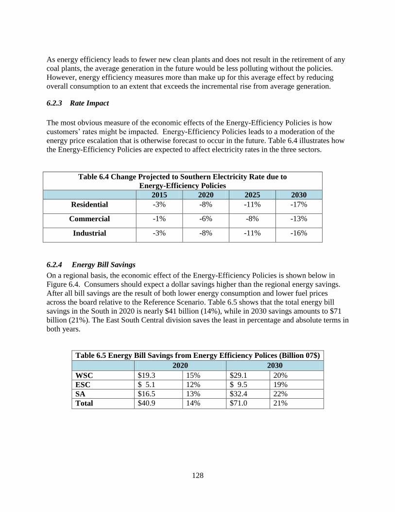
128
As energy efficiency leads to fewer new clean plants and does not result in the retirement of any
coal plants, the average generation in the future would be less polluting without the policies.
However, energy efficiency measures more than make up for this average effect by reducing
overall consumption to an extent that exceeds the incremental rise from average generation.
6.2.3 Rate Impact
The most obvious measure of the economic effects of the Energy-Efficiency Policies is how
customers‟ rates might be impacted. Energy-Efficiency Policies leads to a moderation of the
energy price escalation that is otherwise forecast to occur in the future. Table 6.4 illustrates how
the Energy-Efficiency Policies are expected to affect electricity rates in the three sectors.
Table 6.4 Change Projected to Southern Electricity Rate due to
Energy-Efficiency Policies
2015 2020 2025 2030
Residential -3% -8% -11% -17%
Commercial -1% -6% -8% -13%
Industrial -3% -8% -11% -16%
6.2.4 Energy Bill Savings
On a regional basis, the economic effect of the Energy-Efficiency Policies is shown below in
Figure 6.4. Consumers should expect a dollar savings higher than the regional energy savings.
After all bill savings are the result of both lower energy consumption and lower fuel prices
across the board relative to the Reference Scenario. Table 6.5 shows that the total energy bill
savings in the South in 2020 is nearly $41 billion (14%), while in 2030 savings amounts to $71
billion (21%). The East South Central division saves the least in percentage and absolute terms in
both years.
Table 6.5 Energy Bill Savings from Energy Efficiency Polices (Billion 07$)
2020 2030
WSC $19.3 15% $29.1 20%
ESC $ 5.1 12% $ 9.5 19%
SA $16.5 13% $32.4 22%
Total $40.9 14% $71.0 21%
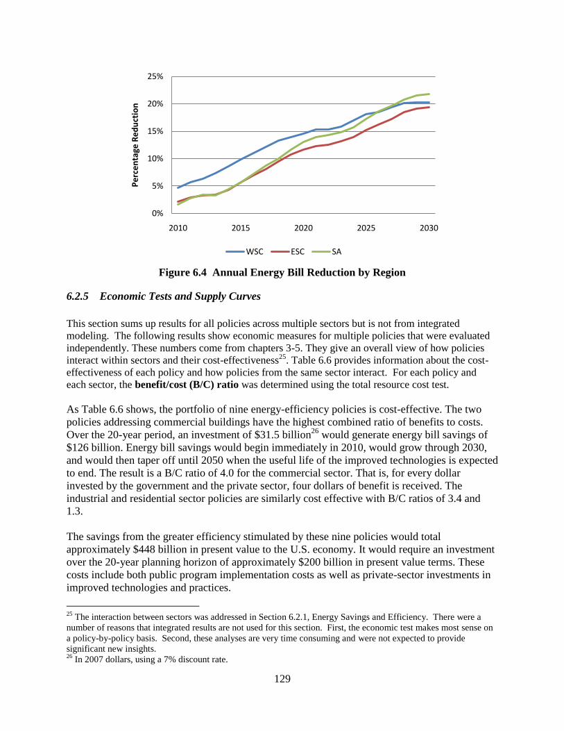
129
Figure 6.4 Annual Energy Bill Reduction by Region
6.2.5 Economic Tests and Supply Curves
This section sums up results for all policies across multiple sectors but is not from integrated
modeling. The following results show economic measures for multiple policies that were evaluated
independently. These numbers come from chapters 3-5. They give an overall view of how policies
interact within sectors and their cost-effectiveness25. Table 6.6 provides information about the cost-
effectiveness of each policy and how policies from the same sector interact. For each policy and
each sector, the benefit/cost (B/C) ratio was determined using the total resource cost test.
As Table 6.6 shows, the portfolio of nine energy-efficiency policies is cost-effective. The two
policies addressing commercial buildings have the highest combined ratio of benefits to costs.
Over the 20-year period, an investment of $31.5 billion26
would generate energy bill savings of
$126 billion. Energy bill savings would begin immediately in 2010, would grow through 2030,
and would then taper off until 2050 when the useful life of the improved technologies is expected
to end. The result is a B/C ratio of 4.0 for the commercial sector. That is, for every dollar
invested by the government and the private sector, four dollars of benefit is received. The
industrial and residential sector policies are similarly cost effective with B/C ratios of 3.4 and
1.3.
The savings from the greater efficiency stimulated by these nine policies would total
approximately $448 billion in present value to the U.S. economy. It would require an investment
over the 20-year planning horizon of approximately $200 billion in present value terms. These
costs include both public program implementation costs as well as private-sector investments in
improved technologies and practices.
25
The interaction between sectors was addressed in Section 6.2.1, Energy Savings and Efficiency. There were a
number of reasons that integrated results are not used for this section. First, the economic test makes most sense on
a policy-by-policy basis. Second, these analyses are very time consuming and were not expected to provide
significant new insights. 26
In 2007 dollars, using a 7% discount rate.
0%
5%
10%
15%
20%
25%
2010 2015 2020 2025 2030
Pe
rce
nta
ge R
ed
uct
ion
WSC ESC SA

130
Table 6.6 Total Resource Cost Tests by Sector (Million 07$)
Residential Sector Policies
NPV Cost NPV Benefit B/C Ratio
Building Codes with
Third-Party
Verification
$10,000
$41,400
4.1
Appliance Incentives
and Standards
$25,500
$7,060
0.3
Expanded
Weatherization
Assistance Program
$5,840
$6,420
1.1
Residential Retrofit
and Equipment
Standards
$86,600
$119,000
1.4
Combined Policies $115,000 $143,000 1.3
Commercial Sector Policies
NPV Cost NPV Benefit B/C Ratio
Tighter Commercial
Appliance Standards
$26,300 $109,000 4.6
Commercial Retrofit
Incentives
$8,540 $20,900 2.4
Combined Policies $31,500 $126,000 4.0
Industrial Sector Policies
NPV Cost NPV Benefit B/C Ratio
Industrial Plant
Utility Upgrades
$10,800
$48,400
4.5
Industrial Process
Improvement Policy
$36,000
$128,811 3.6
Combined Heat and
Power Incentives
$16,900 $11,400
$17,600*
0.67
1.04*
Combined Policies $53,200 $179,000 3.4 * Includes the environmental benefits from CO2 emissions avoided by CHP systems.
The findings of McKinsey's "Unlocking Energy Efficiency in the U.S. Economy" are quite
consistent with these estimates for the South, despite the fact that their analytic approach is quite
different (Granade, et al., 2009). They conclude that by 2020, the United States could cost-
effectively reduce its annual energy consumption by 23 percent from a business-as-usual
projection, saving 9.1 quads of end-use energy. Further, these savings would be worth
approximately $1.2 trillion in present value to the U.S. economy, and would require an initial
upfront investment of about $520 billion. Public costs associated with implementing the policies
needed to achieve these savings are not included in this estimate.
Among the nine individual policies, only two have benefit/cost ratios of less than one –
indicating that they are not cost-effective. These include appliance incentives and standards (with
a B/C ratio of 0.3) and combined heat and power incentives (with a B/C ratio of 0.7). When

131
clothes washers and refrigerators are removed from the suite of appliance standards with
incentives, the B/C ratio rises to 0.7. When carbon dioxide emission reductions are valued (at a
range of $15 per metric ton in 2010 rising to $51 in 2030), both of these policies approach or
exceed the breakeven B/C ratio of 1.
According to the total resource cost test, the most cost-effective policy is tighter commercial
appliance standards (with a B/C ratio of 4.6), followed by B/C ratios of 4.5 for industrial plant
utility upgrades and 4.1 for residential building codes with third party verification. These high
B/C ratios combined with the fact that we examined an incomplete set of policies and
technologies, suggests that greater levels of investment could generate additional, cost-effective
energy savings.
Energy-efficiency supply curves have typically focused on individual technologies. Since the
emphasis of this report is on program achievable energy efficiency potential, we have developed
policy supply curves. The magnitude of energy demand resources that can be achieved by
launching aggressive energy efficiency programs is shown along the horizontal axis, and they are
ordered from the lowest to the highest levelized cost.
The energy supply curve for the South in 2020 (Figure 6.5) illustrates how over 4,300 TBtu of
cost-effective opportunities for energy efficiency could be realized through policy
implementation in 2020. McKinsey‟s 2009 study estimated a slightly smaller energy-efficiency
opportunity in 2020 – 3,650 TBtu (Ostrowski, 2009).
Figure 6.5 Supply Curve Energy-Efficiency Policies in the South in 2020 (RCI Sectors)
The least-cost savings can be achieved in the industrial sector, where over 50% of the potential
would be realized. On the other hand, Residential Retrofit Incentives with Equipment Standards
achieve very little energy efficiency for a much higher price.

132
The electricity efficiency supply curve for the South (Figure 6.6) illustrates how more than 2,100
TBtu of electricity savings could be realized from implementing eight energy-efficiency policies.
(The combined heat and power policy could not be assigned a levelized cost value.) The supply
curve also highlights the large, low-cost potential of industrial efficiency opportunities, which
together could save more than 500 TBtu of electricity for a levelized cost that is significantly
lower than the price of electricity for industrial consumers (6.2 cents/kWh). The next most cost-
effective efficiency option is the commercial standards policy, followed by building codes,
bringing the cumulative savings for these four policies to nearly 900 TBtu. When the retrofit
incentives and equipment standards are added, a large additional savings can be achieved. The
three remaining policies do not save as much electricity, including appliance incentives and
standards, which produce electricity savings at a levelized cost that exceeds the residential price
of electricity (10.5 cents/kWh).
Figure 6.6 Supply Curve for Electricity Efficiency Resources in the South in 2020
(RCI Sectors)
The natural gas supply curve (Figure 6.7) distributes approximately 1,450 TBtu of savings across
the eight efficiency policies. While commercial standards and residential building codes offer the
least-cost natural gas savings, the magnitude of impact of these two policies is limited. Industrial
plant utility upgrades and process improvements are also low-cost, and they offer larger-scale
opportunities for cost-effective natural gas savings in the South.

133
Figure 6.7 Supply Curve for Natural Gas Efficiency in the South in 2020 (RCI Sectors)
6.2.6 Macroeconomic and Job Impacts
To evaluate how the nine energy-efficiency policies might impact levels of employment and
economic activity in the South, we use an Input-Output Calculator developed by the American
Council for an Energy-Efficient Economy (ACEEE) for evaluating macroeconomic and job
impacts of investments in energy efficiency (Laitner and Knight, 2009). The most important
component of the calculator are the South Census Region‟s impact coefficients for 2008
provided by IMPLAN (IMpact Analysis for PLANing). IMPLAN is an econometric modeling
system developed by applied economists at the University of Minnesota and the U.S. Forest
Service. Currently in use by more than 500 organizations, IMPLAN models the trade flow
relationships between businesses and between businesses and final consumers.27
Methodology. The critical statistics for estimating employment impacts are the jobs coefficients,
which represent the number of jobs generated by an investment of $1 million in a particular
industry. These coefficients indicate that an investment of $1 million in the construction and
energy-efficient product manufacturing sectors (which includes both new building and
retrofitting) generated 16.45 jobs in 2008. For the electricity and natural gas sectors, $1 million
generated only 5.63 and 8.43 jobs, respectively. All other sectors of the economy had an average
impact coefficient of 13.86 jobs per million dollars in 2008 (Figure 6.8). The higher labor
intensity indicated by the large jobs coefficient for construction and energy-efficient
manufacturing is one of the indicators that investing in energy efficiency is an engine for job
creation.
27
http://www.massachusetts.edu/econimpact/methodology.html

134
Figure 6.8 GSP, Jobs, and Regional Purchase Coefficients of Economic Sectors in the South
Jobs calculations going forward in time use the same coefficients, but also accounts for an annual
1.9% increase in labor productivity, based on Bureau of Labor Statistics (2009a) estimates.
Also important for estimating regional employment impacts are the Regional Purchase
Coefficients (RPCs). An RPC is the proportion of the total demand for commodities by all users
in the region that is supplied by producers located within the region. Of the four sectors
examined here, the RPC in the South is highest for electricity (0.96) followed by construction
and energy-efficiency product manufacturing (0.86), other sectors (0.75), and natural gas (0.72).
Thus, 86% of the demand for construction and energy-efficiency product manufacturing in the
South is supplied by producers located in the South, while 14% of the demand is satisfied by
import.28
Investment in goods with significant “local” content (i.e., larger RPC‟s) leads to greater
local job creation. Local job growth is particularly large when a high RPC Coefficient is
combined with a high Job Coefficient, as in the case of construction and energy-efficiency
manufacturing.
The critical statistics for estimating impacts on economic activity are the GRP Coefficients,
which represent the value added to the economy per dollar of investment. In 2008 the IMPLAN
GRP coefficients for the South Census Region were 1.09 for construction and energy-efficient
product manufacturing, 1.08 for electricity, 0.98 for natural gas and 1.10 for all other sectors.
(See Table F.3.1 in Appendix F for the aggregation scheme of the sectors in the ACEEE
calculator).
28
These coefficients tend to be smaller and more variable as the size of the region shrinks – e.g., in the analysis of
State impacts.
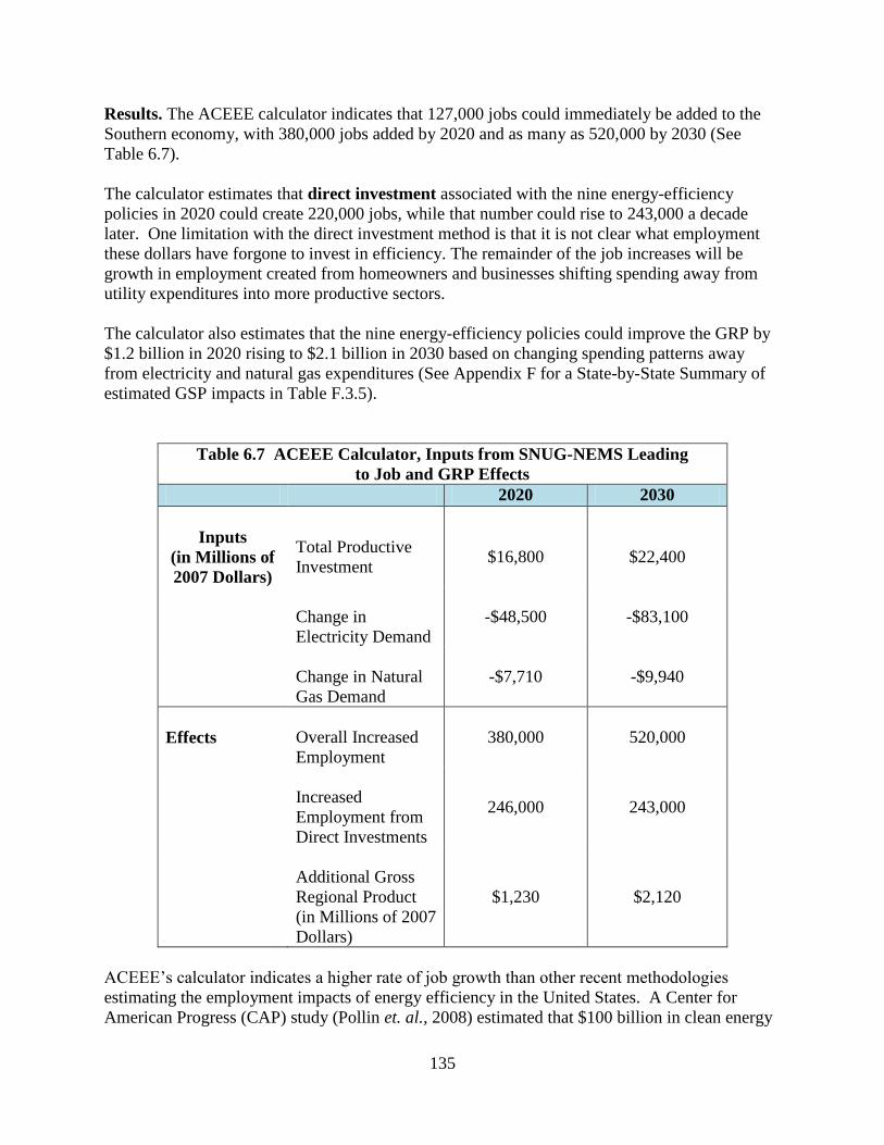
135
Results. The ACEEE calculator indicates that 127,000 jobs could immediately be added to the
Southern economy, with 380,000 jobs added by 2020 and as many as 520,000 by 2030 (See
Table 6.7).
The calculator estimates that direct investment associated with the nine energy-efficiency
policies in 2020 could create 220,000 jobs, while that number could rise to 243,000 a decade
later. One limitation with the direct investment method is that it is not clear what employment
these dollars have forgone to invest in efficiency. The remainder of the job increases will be
growth in employment created from homeowners and businesses shifting spending away from
utility expenditures into more productive sectors.
The calculator also estimates that the nine energy-efficiency policies could improve the GRP by
$1.2 billion in 2020 rising to $2.1 billion in 2030 based on changing spending patterns away
from electricity and natural gas expenditures (See Appendix F for a State-by-State Summary of
estimated GSP impacts in Table F.3.5).
Table 6.7 ACEEE Calculator, Inputs from SNUG-NEMS Leading
to Job and GRP Effects
2020 2030
Inputs
(in Millions of
2007 Dollars)
Total Productive
Investment
$16,800
$22,400
Change in
Electricity Demand
-$48,500 -$83,100
Change in Natural
Gas Demand
-$7,710 -$9,940
Effects
Overall Increased
Employment
380,000 520,000
Increased
Employment from
Direct Investments
246,000 243,000
Additional Gross
Regional Product
(in Millions of 2007
Dollars)
$1,230 $2,120
ACEEE‟s calculator indicates a higher rate of job growth than other recent methodologies
estimating the employment impacts of energy efficiency in the United States. A Center for
American Progress (CAP) study (Pollin et. al., 2008) estimated that $100 billion in clean energy
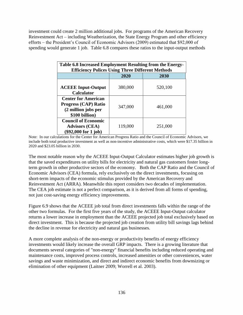
136
investment could create 2 million additional jobs. For programs of the American Recovery
Reinvestment Act – including Weatherization, the State Energy Program and other efficiency
efforts – the President‟s Council of Economic Advisors (2009) estimated that $92,000 of
spending would generate 1 job. Table 6.8 compares these ratios to the input-output methods
Table 6.8 Increased Employment Resulting from the Energy-
Efficiency Polices Using Three Different Methods
2020 2030
ACEEE Input-Output
Calculator
380,000 520,100
Center for American
Progress (CAP) Ratio
(2 million jobs per
$100 billion)
347,000 461,000
Council of Economic
Advisors (CEA)
($92,000 for 1 job)
119,000 251,000
Note: In our calculations for the Center for American Progress Ratio and the Council of Economic Advisors, we
include both total productive investment as well as non-incentive administrative costs, which were $17.35 billion in
2020 and $23.05 billion in 2030.
The most notable reason why the ACEEE Input-Output Calculator estimates higher job growth is
that the saved expenditures on utility bills for electricity and natural gas customers foster long-
term growth in other productive sectors of the economy. Both the CAP Ratio and the Council of
Economic Advisors (CEA) formula, rely exclusively on the direct investments, focusing on
short-term impacts of the economic stimulus provided by the American Recovery and
Reinvestment Act (ARRA). Meanwhile this report considers two decades of implementation.
The CEA job estimate is not a perfect comparison, as it is derived from all forms of spending,
not just cost-saving energy efficiency improvements.
Figure 6.9 shows that the ACEEE job total from direct investments falls within the range of the
other two formulas. For the first five years of the study, the ACEEE Input-Output calculator
returns a lower increase in employment than the ACEEE projected job total exclusively based on
direct investment. This is because the projected job creation from utility bill savings lags behind
the decline in revenue for electricity and natural gas businesses.
A more complete analysis of the non-energy or productivity benefits of energy efficiency
investments would likely increase the overall GRP impacts. There is a growing literature that
documents several categories of "non-energy" financial benefits including reduced operating and
maintenance costs, improved process controls, increased amenities or other conveniences, water
savings and waste minimization, and direct and indirect economic benefits from downsizing or
elimination of other equipment (Laitner 2009; Worrell et al. 2003).

137
Figure 6.9 Increased Employment Impacts from Energy-Efficiency Policies for the Region *Includes jobs from direct investment and changes in electricity
Shifting revenues from the non-labor intensive energy production industries to more labor
intensive industries can create long-term job growth prospects, particularly during periods of
high unemployment when labor is underutilized. The seasonally adjusted unemployment rate in
the South Census Region was 9.6% in December 2009 (Bureau of Labor Statistics, 2009b).
While this is lower than the national rate of 10.0%, the District of Columbia, Florida, North
Carolina, and South Carolina all had over 11% unemployment.
While energy-efficiency policies may not be an instantaneous or complete solution to the current
financial difficulties of the South, our analysis suggests that the public and private investments
stimulated by the nine energy-efficiency policies will have a positive impact on employment and
macroeconomic growth over the next two decades.
6.3 SENSITIVITY ANALYSIS
We use sensitivity analysis to help capture uncertainty associated with SNUG-NEMS
forecasting. Sensitivity analysis helps practitioners and policymakers understand the implications
of key assumptions, such as the future price of carbon or future technology breakthroughs.
The major topic chosen for sensitivity analysis of the Energy-Efficiency Policies was a case where
a price is placed on carbon emissions, starting at $15/tonne CO2 rising to $51/tonne in 2030. This
sensitivity is called the Carbon Constrained Future (CCF). This sensitivity was chosen because
regional and national regulation of greenhouse gases has been prominent and seems likely to
affect the marketplace for energy-efficient technologies and the response to energy policies. To

138
evaluate the combined effect of Energy-Efficiency Policies with a carbon constraint, we modeled
CCF alone and combined with the Energy-Efficiency Policies. As mentioned in Chapter 2 there
will be four scenarios compared in this section: Reference, Reference with Energy-Efficiency
Policies, CCF, and CCF with Energy-Efficiency Policies.
6.3.1 Elements of the CCF Sensitivity
The CCF parameters include a very basic modeling of limiting greenhouse emissions, because
this is not meant to be an analysis of any particular aspects of potential greenhouse gas
legislation, many others have done that. EPA (2009) conducted a holistic estimate of greenhouse
gas emissions and possible means of reduction in the U.S. McKinsey & Company (2008), from
an economics perspective, estimated the U.S. greenhouse gas emission potential and some of the
associated costs. In addition, the Center for Climate Strategies (2009) examined the greenhouse
gas reduction strategies and potentials in the South. Further, a major report released by ACEEE
in 2008 documents the large economic development contribution of productive investments in
green technologies, which will likely be seen in a carbon-constrained future (Laitner, 2008).
Therefore, unlike anything being discussed in Congress, our CCF scenario is purposely
simplistic which has its limitations, but also serves the purpose of keeping the scenario
straightforward and simple. The main components and caveats include:
Modeling a modest emissions reduction by picking a carbon price that is within EPA‟s
(2009) range of allowance prices ($15 to $51).29
No international offsets, banking, or borrowing.
Allowance revenues are not put into R & D or Energy Efficiency programs.
A portion of revenues are distributed to Load Distribution Companies (LDCs) in order to
offset price increases that consumers would otherwise face30
. This has the side-effect of
reducing the market signal to consumers.
Figure 6.10 shows greenhouse gas emissions of CCF scenario relative to the Reference Scenario,
both in the absence of Energy-Efficiency Policies, leading to 26% less emissions in 2030 from
three demand sectors. Compared to Figure 6.11 which presents the energy consumption in CCF
and Reference Scenarios, the energy savings from CCF are less pronounced (4%) than the
emissions effect. The reason for this is that carbon constraints will first lead to cleaner fuels
being used before reducing total consumption31
.
29
Appendix F Figure F.2.1 illustrates the change of allowance price over years. 30
Appendix B Table B.1 shows the annual allowance given to LDCs. 31
In the EIA‟s analysis of ACESA, they project that in most cases between 6 and 85 percent of existing coal power
plants will be retired by 2030, and that the capacity will be replaced by nuclear, renewable, and coal plants equipped
with CCS. It is projected that annual electricity demand growth will decline from 0.9% to 0.64% between 2007 and
2030 (EIA, 2009i).

139
Figure 6.10 Southern CO2 Emissions Divergence for Sensitivity Analysis
Figure 6.11 Southern Energy Divergence for Sensitivity Analysis
Figure 6.12, which shows the forecast for new capacity in 2030 for the Reference Scenario
compared to the CCF. Most noticeable is that the CCF scenario has increased the nuclear
generating capacity by nearly 44 GW while lowering the combined cycle and combustion
turbine/diesel by over 17 GW each. However, capacity is largely unchanged (marginally higher)
because the CCF effect on total demand is secondary to its effect on fuel type associated with
generation. In both scenarios, more than 15 GW of oil and gas steam generation are retired.
0
200
400
600
800
1,000
1,200
1,400
1,600
1,800
2,000
2010 2015 2020 2025 2030
MM
T C
O2
Reference Scenario CCF
25,000
27,000
29,000
31,000
33,000
35,000
37,000
2010 2015 2020 2025 2030
Trill
ion
Btu
Reference Scenario CCF

140
Figure 6.12 Generating Capacity Installed in 2030 Beyond 2010
Comparing the Reference Scenario and CCF
The next section addresses the question of whether implementing the Energy-Efficiency Policies
under a carbon constrained future leads to similar or different conclusions regarding efficiency
potential and economics than previously discussed in section 6.2.
6.3.2 Energy-Efficiency Policies and CCF
The main conclusion of the sensitivity analysis is that Energy-Efficiency Policies reduce energy
consumption even in a carbon constrained future, when the higher price of fossil fuels has
already lowered the overall consumption. When combined, the Energy-Efficiency Policies lower
energy consumption still further.
This section will attempt to point out how and why CCF and Energy-Efficiency Policies interact.
The energy interactions seem to be limited because at the chosen levels the CCF primarily leads
to lower emissions and higher energy rates, and these rate increases are below the threshold that
leads to significant consumer efficiency choices.
Energy Savings. Figure 6.13 shows that the predominate driver of reduced consumption is
Energy-Efficiency Policies, while this CCF adds only a few percent of further reductions. There
seems to be little synergy or redundant savings at these levels. Measuring the energy savings
from the nine policies added to either the CCF or Reference Scenario reveals a very similar
-20
0
20
40
60
80
Reference CCF
GW
Coal Oil & NG Steam Combined Cycle
Comb Turbine/Diesel Nuclear Power Renewables
49 GW new Capacity net52 GW new Capacity net
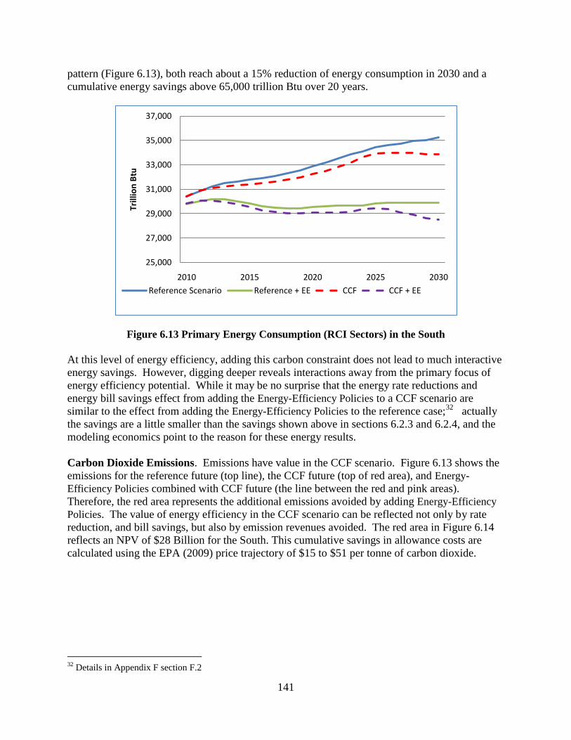
141
pattern (Figure 6.13), both reach about a 15% reduction of energy consumption in 2030 and a
cumulative energy savings above 65,000 trillion Btu over 20 years.
Figure 6.13 Primary Energy Consumption (RCI Sectors) in the South
At this level of energy efficiency, adding this carbon constraint does not lead to much interactive
energy savings. However, digging deeper reveals interactions away from the primary focus of
energy efficiency potential. While it may be no surprise that the energy rate reductions and
energy bill savings effect from adding the Energy-Efficiency Policies to a CCF scenario are
similar to the effect from adding the Energy-Efficiency Policies to the reference case;32
actually
the savings are a little smaller than the savings shown above in sections 6.2.3 and 6.2.4, and the
modeling economics point to the reason for these energy results.
Carbon Dioxide Emissions. Emissions have value in the CCF scenario. Figure 6.13 shows the
emissions for the reference future (top line), the CCF future (top of red area), and Energy-
Efficiency Policies combined with CCF future (the line between the red and pink areas).
Therefore, the red area represents the additional emissions avoided by adding Energy-Efficiency
Policies. The value of energy efficiency in the CCF scenario can be reflected not only by rate
reduction, and bill savings, but also by emission revenues avoided. The red area in Figure 6.14
reflects an NPV of $28 Billion for the South. This cumulative savings in allowance costs are
calculated using the EPA (2009) price trajectory of $15 to $51 per tonne of carbon dioxide.
32
Details in Appendix F section F.2
25,000
27,000
29,000
31,000
33,000
35,000
37,000
2010 2015 2020 2025 2030
Trill
ion
Btu
Reference Scenario Reference + EE CCF CCF + EE

142
Figure 6.14 Emissions and Allowance Revenue with CCF
While energy savings are not interactive between the CCF and the policies, emissions reductions
are. Figure 6.15 shows that combining the emissions levels for the four scenarios under
discussion. In the short term, through 2020, the CCF and Energy-Efficiency Policies in and of
themselves, lead to similar emissions reductions and the combination of the two seems to reach
an additive level that might be expected without any interactions. After 2023 or so, CCF
emissions continue to decline, but when CCF and Energy-Efficiency Policies are combined the
emissions effect starts to diminish. At first, energy efficiency leads to less fossil generation, but
after a while, energy efficiency more and more leads to less clean generation (less nuclear and
renewable). This is reflected below as the dotted lines begin to converge after 2024.
Figure 6.15 Carbon Dioxide Emissions with Energy-Efficiency Policies
0
200
400
600
800
1,000
1,200
1,400
1,600
1,800
2,000
2010 2015 2020 2025 2030
MM
T C
O2
CCF CCF + EE Reference Scenario
1960 MMT Cumulative$ 28 Billion
1,000
1,100
1,200
1,300
1,400
1,500
1,600
1,700
1,800
1,900
2010 2015 2020 2025 2030
MM
T C
O2
Reference Scenario Reference +EE CCF CCF + EE

143
Generating Capacity
Emissions limits, as discussed above, transform power plant fuels but do not lead to much energy
savings in and of it itself. Net capacity growth, beyond 2010, for the four scenarios is shown in
Figure 6.15. As noted regarding consumption, capacity is also about the same regardless of a
CCF, but the fuel mix is quite different when under the CCF scenarios.
In a CCF future, nuclear replaces the new combined cycle and coal plants and some of the
combustion turbines built in a Reference future. In the absence of Energy-Efficiency Policies,
over 50 GW of nuclear power would be built by 2030. Implementing Energy-Efficiency Policies
in this CCF scenario, reduces by half the new nuclear power built. Some renewable plants are
also built to replace retiring generators, but the net capacity change is a reduction of 12 GW in
the Southern NERC regions. Energy-Efficiency Policies mean 64 - 68 GW less capacity in the
Southern NERCs by 2030.
Figure 6.15 Southern NERC Incremental Generating Capacity in 2030 beyond 2010,
The change in number of plants built and retired for CCF with and without Energy-Efficiency
Policies is shown in Appendix Table F.2.2.
-40
-20
0
20
40
60
80
Reference CCF Reference + EE CCF + EE
GW
Coal Oil & NG Steam Combined Cycle
Comb Turbine/Diesel Nuclear Power Renewables
49 GW New Capacity Net
52 GW New Capacity Net
12 GW Less NewCapacity Net
19 GW Less New Capacity Net
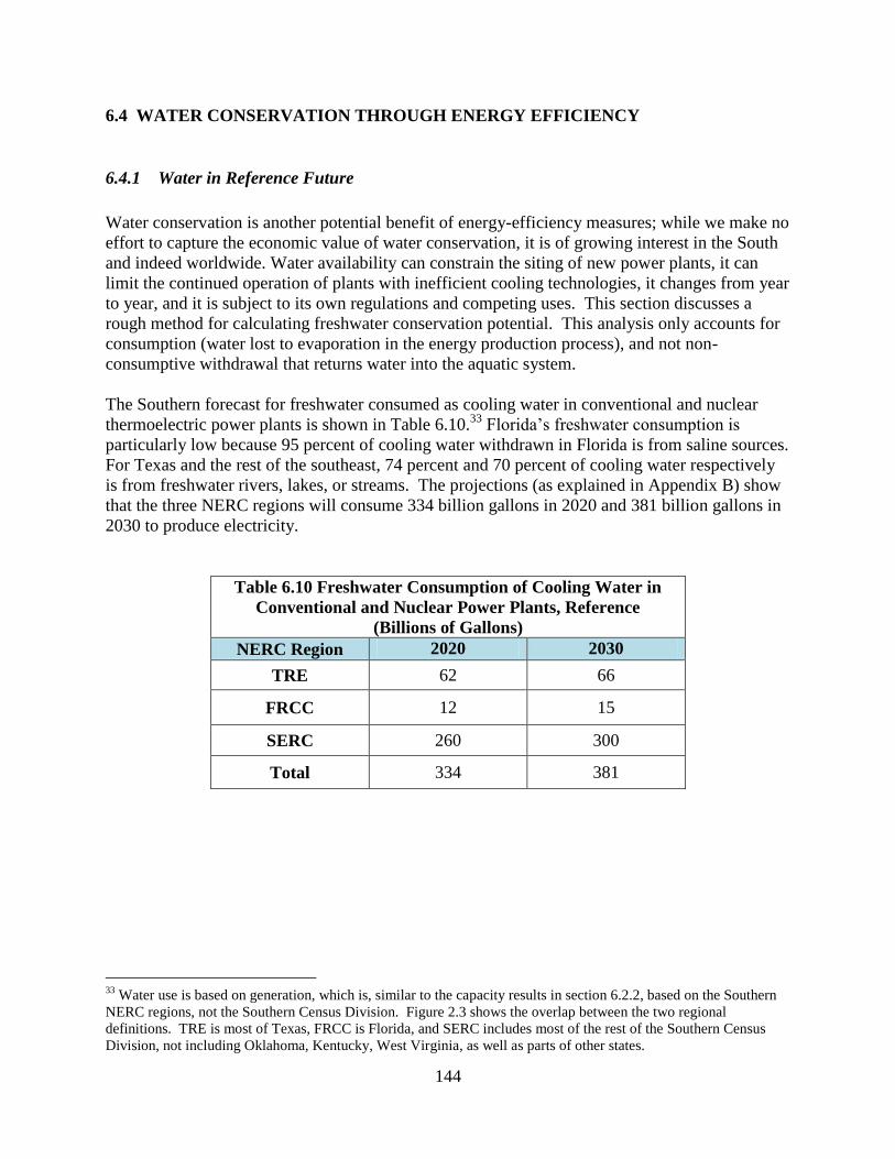
144
6.4 WATER CONSERVATION THROUGH ENERGY EFFICIENCY
6.4.1 Water in Reference Future
Water conservation is another potential benefit of energy-efficiency measures; while we make no
effort to capture the economic value of water conservation, it is of growing interest in the South
and indeed worldwide. Water availability can constrain the siting of new power plants, it can
limit the continued operation of plants with inefficient cooling technologies, it changes from year
to year, and it is subject to its own regulations and competing uses. This section discusses a
rough method for calculating freshwater conservation potential. This analysis only accounts for
consumption (water lost to evaporation in the energy production process), and not non-
consumptive withdrawal that returns water into the aquatic system.
The Southern forecast for freshwater consumed as cooling water in conventional and nuclear
thermoelectric power plants is shown in Table 6.10.33
Florida‟s freshwater consumption is
particularly low because 95 percent of cooling water withdrawn in Florida is from saline sources.
For Texas and the rest of the southeast, 74 percent and 70 percent of cooling water respectively
is from freshwater rivers, lakes, or streams. The projections (as explained in Appendix B) show
that the three NERC regions will consume 334 billion gallons in 2020 and 381 billion gallons in
2030 to produce electricity.
Table 6.10 Freshwater Consumption of Cooling Water in
Conventional and Nuclear Power Plants, Reference
(Billions of Gallons)
NERC Region 2020 2030
TRE 62 66
FRCC 12 15
SERC 260 300
Total 334 381
33
Water use is based on generation, which is, similar to the capacity results in section 6.2.2, based on the Southern
NERC regions, not the Southern Census Division. Figure 2.3 shows the overlap between the two regional
definitions. TRE is most of Texas, FRCC is Florida, and SERC includes most of the rest of the Southern Census
Division, not including Oklahoma, Kentucky, West Virginia, as well as parts of other states.

145
6.4.2 Water Conservation from the Energy-Efficiency Policies
From the implementation of our water calculator (more details in section 2.7 and Appendix F),
we found that energy efficiency could avoid the consumption of significant quantities of
freshwater across the South (Table 6.11). The nine energy-efficiency policies alone, could avoid
generation that in turn would save the South 8.6 billion gallons of water in 2020 and 20.1 billion
gallons in 2030.
Table 6.11 Freshwater Saved with Energy-Efficiency Policies
Comparison In 2020 In 2030
Billions of Gallons Saved 8.6 20.1
2009 to 2020 2020 to 2030
Projected Change in
Consumption (Reference
Case)
4.6% 12.2%
Cumulative Avoided
Increase from Policies
3% 7%
Cumulative Avoided
Marginal Increase from
Policies
56% 43%
On a percentage basis, the Energy-Efficiency Policies could reduce more than half of the
projected growth in cooling water needs for conventional and nuclear power from 2009 to 2020
and 43% of the projected growth for 2020 to 2030. Table 6.12 shows the new consumption
forecasts with energy-efficiency policies for 2020 and 2030.
Table 6.12 Freshwater Consumption of Cooling Water in
Conventional and Nuclear Power Plants, Reference with
Energy-Efficiency Policies
(Billions of Gallons)
NERC Region 2020 2030
TRE 62 65
FRCC 12 14
SERC 252 282
Total 326 361
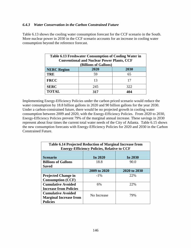
146
6.4.3 Water Conservation in the Carbon Constrained Future
Table 6.13 shows the cooling water consumption forecast for the CCF scenario in the South.
More nuclear power in 2030 in the CCF scenario accounts for an increase in cooling water
consumption beyond the reference forecast.
Table 6.13 Freshwater Consumption of Cooling Water in
Conventional and Nuclear Power Plants, CCF
(Billions of Gallons)
NERC Region 2020 2030
TRE 59 65
FRCC 13 17
SERC 245 322
TOTAL 317 404
Implementing Energy-Efficiency Policies under the carbon priced scenario would reduce the
water consumption by 18.8 billion gallons in 2020 and 90 billion gallons for the year 2030.
Under a carbon-constrained future, there would be no projected growth in cooling water
consumption between 2009 and 2020, with the Energy-Efficiency Policies. From 2020 to 2030,
Energy-Efficiency Policies prevent 79% of the marginal annual increase. These savings in 2030
represent about four times the current total water needs of the City of Atlanta. Table 6.15 shows
the new consumption forecasts with Energy-Efficiency Policies for 2020 and 2030 in the Carbon
Constrained Future.
Table 6.14 Projected Reduction of Marginal Increase from
Energy-Efficiency Policies, Relative to CCF
Scenario
In 2020
In 2030
Billions of Gallons
Saved
18.8 90.0
2009 to 2020 2020 to 2030
Projected Change in
Consumption (CCF)
-1% 22%
Cumulative Avoided
Increase from Policies
6% 22%
Cumulative Avoided
Marginal Increase from
Policies
No Increase 79%

147
Table 6.15 Freshwater Consumption of Cooling Water in
Conventional and Nuclear Power Plants, CCF with Energy-
Efficiency Policies
(Billions of Gallons)
NERC Region 2020 2030
TRE 54 48
FRCC 12 16
SERC 233 250
TOTAL 298 314
Table 6.16 provides a summary of the forecasts for the different scenarios. It shows clearly that
freshwater consumption of cooling water in conventional and nuclear power plants in the South
is lowest under a carbon-constrained scenario with energy-efficiency policies. Although fresh
water savings as a percentage of reference case consumption are not as high as the percent
energy savings, water conservation is a significant benefit of energy efficiency.
Table 6.16 Freshwater Consumption of Cooling Water in
Conventional and Nuclear Power Plants, Summary of
Scenarios for the TRE, FRCC and SERC NERC Regions
(Billions of Gallons)
NERC Region 2020 2030
Reference Case 334 381
Reference Case
with EE Policies 326 361
CCF 317 404
CCF with EE
Policies 298 314
Further research and analysis is likely to show other water conservation co-benefits from energy
efficiency.
The weatherization and retrofit programs discussed in this report may include water
conservation components (such as instillation of low-flow toilets) on top of the energy
saving measures.
Power-plant water withdrawals would be reduced as the result of energy-efficiency
policies, but this is difficult to characterize due to the high variability between power
plants in this area. Water withdrawals, even where used cooling water is returned to the
environment, can have a deleterious impact on freshwater ecosystems.
Energy efficiency may also lead to reductions in mining and extraction, thereby
preventing degradation of waterways from coal-ash and other harmful materials.

148
As noted in a recent Government Accountability Office report (2009), available data on power-
plant water consumption is relatively incomplete. Policy-makers and researchers have only
recently begun focusing on the energy-water nexus regarding the significant benefit of water
conservation from energy efficiency, but it could be a useful tool for integrated resource
planning.
6.5 CONCLUSIONS
The Energy-Efficiency Policies modeled in this study suggest the potential for significant energy
savings in the South – either in a reference future or in a future where carbon emissions are
priced. In 2030, more than 5,600 trillion Btu could be saved, with or without a future carbon
constraint, and the cumulative energy savings from 2010 to 2030 could be more than 65,000
trillion Btu. These results are in line with estimates from other major studies.
Our analysis has documented that Energy-Efficiency Policies generally dampen energy price
increases. Rate reductions coupled with energy savings leads to significant energy bill savings.
In 2030, the South could realize $68 billion energy bill saving in the CCF scenario and more than
$70 billion in the reference case, which each represent more than 20% of total expenses.
In addition, it is estimated that 49 GW of new power plant capacity would not need to be built in
the South, if aggressive Energy-Efficiency Policies were implemented instead. At the same time,
Energy-Efficiency Policies could conserve 90 billion gallons of water that would otherwise be
consumed in processes related to energy generation, in the year 2030.
Though our Energy-Efficiency Policies result in significant energy savings, it is conservative in
many respects, as is illustrated in Figure 6.17. On a percentage basis, the energy savings
estimated in this report are lower than those of many other studies of the South. In some cases
this is because we‟re comparing our estimates of achievable economic potential with NPV-
positive estimates that do not account for shortfalls in implementation (McKinsey). In other
cases, the higher potential is produced in part by the assumption of major technology
improvements from large-scale R&D investments (IWG).

149
Figure 6.17: Comparisions with Other Studies for 2020 Savings
Our analysis is also limited by a range of simplifying assumptions and omissions. A number of
these are described below.
Limited assumptions are made about the technology improvements that could emerge
from expanded R&D investments. Greater resources could be committed to energy
efficiency R&D in the future if, for instance, a price were to be put on carbon, which is
also not fully explored in this study. While we do examine a simplified carbon
constrained future scenario, it does not include many policy dimensions currently under
debate such as the use of domestic and international carbon offsets and the creation of a
national trading program for carbon credits and energy efficiency certificates.
Many aspects of consumer behavior are treated inadequately. For example, we do not
consider the transformational influence of an increased public commitment to clean
energy as a means of addressing global climate change. Indeed, we do not consider the
impacts of a 2 degree Centigrade rise in global temperatures by mid-century, on
requirements for air conditioning and the availability of water-demanding forms of
electricity generation including hydropower, coal, and nuclear plants.
Several sectors and technologies are insufficiently addressed (including new construction
of commercial buildings, residential lighting technologies, and several forms of recycled
0
5
10
15
20
25
30
35
Residential Commercial Industrial
Per
cen
tag
e E
ner
gy
Sa
vin
gs
Energy Efficiency in the South (2009) IWG (2000) Moderate
Brown et al. (2009) IWG (2000) Advanced
Beck et al. (2002) McKinsey (2009)

150
energy in industry). More comprehensive coverage of these would increase our estimates
of energy efficiency potential.
Transportation energy efficiency is omitted from our analysis, and yet it could have a
large impact on the operation of the three sectors we do address. For example, the
electrification of transportation in the U.S. could escalate power prices, creating greater
demand for energy-saving devices. Several other synergies between policies are also not
fully elaborated such as workforce development issues including possible economies of
scale in training the future green workforce.
In the future, sensitivity analysis taking these factors into account should further explore the
additional potential for energy efficiency under a range of assumptions about future carbon
policies and climate conditions.
151
References
ACEEE (2009, June 29, 2009). "President Obama Announces New Light Bulb Standards:
Biggest Energy Saver in History of Energy Department." 2009.
Retrieved from: http://www.aceee.org/press/0906lighting.htm
Advanced Fiber Technology. (nd). Dynamic Cellulose Insulation (Blend with Phase Change
Material). Retrieved on October 29, 2009 from:
http://www.advancedfiber.com/dynamicci.pdf.
AISI. 2005. Saving One Barrel of Oil per Ton. Washington, DC: AISI. October.
Amamath, A. (2009, December 10). Personal Communication. Electric Power Research Institute.
Amann, J.T., and E. Mendelsohn. 2005. “Comprehensive Commercial Retrofit Programs: A
Review of Activity and Opportunities.” ACEEE A052.
www.aceee.org/pubs/a052.pdf?CFID=3441108&CFTOKE N=85072968
American Clean Energy and Security Act of 2009 (ACESA). 2009. HR 2454.
http://energycommerce.house.gov/index.php?option=com_content&task=view&id=1560
#toc0
American Recovery and Reinvestment Act of 2009. (2009). Retrieved on March 30, 2009 from:
http://frwebgate.access.gpo.gov/cgi-bin/getdoc.cgi?dbname=111_cong_bills&docid=
f:h1enr.pdf.
Appliance Standard Awareness Project (ASAP). 2009. Status of State Adoption if Energy
Efficiency Standards.
http://www.standardsasap.org/state/index.htm
Appliance Standards Awareness Project (ASAP). (2009). Federal Standards. Retrieved on
October 19, 2009 from: http://www.standardsasap.org/federal.htm.
Beck, Fredric, Damian Kostiuk, Tim Woolf, David White, Monserrat Ramio, Michael Brower,
and Virinder Singh. 2002. Powering the South: A Clean Affordable Energy Plan for the
Southern United States. Renewable Energy Policy Project.
http://www.repp.org/articles/static/1/binaries/pts_repp_book.pdf
Brown, M.., M. Levine, W. Short, and J. Koomey. 2001. Scenarios for a clean energy future.
Energy Policy 29(14):1179-1196.
Brown, Marilyn and Sharon “Jess” Chandler. 2008. “Governing Confusion: How
Statutes, Fiscal Policy, and Regulations Impede Clean Energy Technologies,” Stanford
Law and Policy Review,(19) 3: 472-509.
http://slpr.stanford.edu/previous/Volume19.html#Issue3

152
Brown, Marilyn A., Jess Chandler, Melissa Lapsa, and Moonis Ally. 2009a. Making Homes Part
of the Climate Solution. Oak Ridge National Laboratory, ORNL/TM-2009/104, June,
http://www.ornl.gov/sci/eere/PDFs/CCTP_PolicyOptions_200906.pdf.
Brown, Marilyn A., John A. “Skip” Laitner, Sharon “Jess” Chandler, Elizabeth D. Kelly, Shruti
Vaidyanathan, Vanessa McKinney, Cecelia “Elise” Logan, and Therese Langer. 2009b.
Energy Efficiency in Appalachia: How much more is available, at what cost, and by
when? Appalachian Regional Commission and Southeast Energy Efficiency Alliance.
Brown, Marilyn A., Frank Southworth, and Andrea Sarzynski. 2009. “The Geography of
Metropolitan Carbon Footprints,” Policy and Society 27: 285-304.
Bureau of Labor Statistics. 2009a. Labor Productivity and Costs. Washington, DC: Bureau of
Labor Statistics. Accessed October 2009.
http://www.bls.gov/lpc/.
Bureau of Labor Statistics. 2009b. Regional and State Unemployment. Washington, DC:
Bureau of Labor Statistics. Accessed 1/28/10.
http://www.bls.gov/news.release/pdf/laus.pdf.
California Energy Commission. (2001). California Standard Practice Manual: Economic
Analysis of Demand-Side Programs and Projects. Retrieved on August 11, 2009 from:
http://www.energy.ca.gov/greenbuilding/documents/background/07-
J_CPUC_STANDARD_PRACTICE_MANUAL.PDF
CCTP, 2010. Brown, Marilyn, Roderick Jackson, Matt Cox and Benjamin Deitchman. Policy
Options for Energy Efficiency in the Industrial Sector. Oak Ridge, TN: Oak Ridge
National Laboratory, forthcoming.
Census Bureau. (2009a). GCT-T1-R. Population Estimates. Retrieved from:
http://factfinder.census.gov/servlet/GCTTable?_bm=y&-geo_id=01000US&-
_box_head_nbr=GCT-T1-R&-ds_name=PEP_2008_EST&-format=US-40S.
Census Bureau. (2009b). Historical Census of Housing Tables: Units in Structure. Retrieved
from: http://www.census.gov/hhes/www/housing/census/historic/ units.html.
Census Bureau. (2009c). Current Population Survey, 2009 Annual Social and Economic
Supplement. Retrieved on September 11, 2009 from:
http://www.census.gov/hhes/www/cpstables/032009/pov/new46_135150_01.htm.
Center for Climate Strategies (2009) Southern Regional Economic Assessment of Climate Policy
Options and Review of Economic Studies of Climate Policy
Committee on Climate Change Science and Technology Integration (CCCSTI). 2009. “Strategies
for the Commercialization and Deployment of Greenhouse Gas Intensity-Reducing
Technologies and Practices.” Washington, DC: U.S. Department of Energy, DOE/PI-
0007. http://www.climatetechnology.gov/Strategy-Intensity-Reducing-Technologies.pdf

153
Council of Economic Advisors. (2009). Estimates of Job Creation from the American Recovery
and Reinvestment Act of 2009. Executive Office of the President, Washington, DC.
Cymbalsky, J. (October 1, 2009). E-mail communication. Recessed Can Lighting Standard. O.
Soumonni and J. Wang.
Cymbalsky, J. (2009). Recessed Can Lighting Standard. O. Soumonni and J. Wang.
DSIRE. (2009). Rules, Regulations, & Policies for Energy Efficiency. Retrieved on
October 19, 2009 from: http://www.dsireusa.org/summarytables/rrpee.cfm.
Department for Environment, Food and Rural Affairs (DEFRA). 2007. “Public Understanding of
Sustainable Energy Consumption in the Home.”
http://randd.defra.gov.uk/Document.aspx?Document=EV02046_6701_FRP.pdf
Eldridge, M., A. deLaski, et al. (2006). Opportunities for Appliance and Equipment Efficiency
Standards in Texas.
Eldridge, Maggie, R. Neal Elliott, and Max Neubauer. 2008. “State-Level Energy
Efficiency Analysis: Goals, Methods and Lessons Learned.” Proceedings of the 2008
ACEEE Summer Study on Energy Efficiency in Buildings. Washington, DC: American
Council for an Energy-Efficient Economy.
Electric Power Research Institute. (2009a). Assessment of Achievable Potential from Energy
Efficiency and Demand Response Programs in the U.S. (2010-2030). Retrieved on
December 20, 2009 from:
http://mydocs.epri.com/docs/public/000000000001018363.pdf.
Electric Power Research Institute. (2009b). The Potential to Reduce CO2 Emissions by
Expanding End-Use Applications of Electricity. Retrieved on March 12, 2010 from:
http://my.epri.com/portal/server.pt?Abstract_id=000000000001018871.
Energy and Environmental Analysis Inc. (EEA). 2009. Combined Heat and Power Installation
Database.
http://www.eea-inc.com/chpdata/index.html
Energy Independence and Security Act (EISA). 2007. Subtitle B - Lighting Energy Efficiency.
U. S. Congress. Washington D.C. H.R.6: p.88.
Energy Information Administration (EIA). 2003. National Energy Modeling System: An
Overview 2003.
http://www.eia.doe.gov/oiaf/aeo/overview/pdf/international.pdf
Energy Information Administration (EIA). 2006. Manufacturing Energy Consumption Survey
(MECS).
http://www.eia.doe.gov/emeu/mecs/mecs2006/2006tables.html
154
Energy Information Administration (EIA). 2007. Annual Energy Outlook 2007.
http://tonto.eia.doe.gov/ftproot/forecasting/0383(2007).pdf
Energy Information Agency (EIA). 2008. Annual Energy Outlook 2008.
http://www.eia.doe.gov/oiaf/aeo/index.html
Energy Information Agency (EIA). 2008. Model Documentation Report: Industrial Sector
Demand Module of the National Energy Modeling System
Energy Information Administration (EIA). 2009. Annual Energy Outlook 2009 (AEO2009).
http://www.eia.doe.gov/oiaf/aeo/pdf/0383(2009).pdf
Energy Information Administration. (2009a). Table S-1 Energy Consumption Estimates by
Source and End-Use Sector, 2007. Retrieved from:
http://www.eia.doe.gov/emeu/states/sep_sum/html/pdf/sum_btu_1.pdf.
Energy Information Administration. (2009b). Table S4. Residential Sector Energy Consumption
Estimates, 2007. Retrieved from: http://www.eia.doe.gov/emeu/
states/hf.jsp?incfile=sep_sum/plain_html/sum_btu_res.html.
Energy Information Administration. (2009c). Table S8. Electric Power Sector Consumption
Estimates, 2007. Retrieved from: http://www.eia.doe.gov/emeu/
states/sep_sum/html/pdf/sum_btu_eu.pdf.
Energy Information Administration. (2009d). State Energy Data System. Retrieved on August 6,
2009 from: http://www.eia.doe.gov/emeu/states/_seds.html.
Energy Information Administration. (2009e). Assumptions to the Annual Energy Outlook 2009:
Residential Demand Module. Retrieved on August 7, 2009 from:
http://www.eia.doe.gov/oiaf/aeo/assumption/residential.html.
Energy Information Administration. (2009f). 2005 Residential Energy Consumption Survey
Detailed Tables: Table US1. Total Energy Consumption, Expenditures, and Intensities,
2005, Part 2: Household Characteristics. Retrieved from:
http://www.eia.doe.gov/emeu/recs/recs2005/c&e/summary/pdf/tableus1part2.pdf.
Energy Information Administration. (2009g). Natural Gas Navigator: Natural Gas Prices.
Retrieved from: http://tonto.eia.doe.gov/dnav/ng/ng_pri_sum_dcu_STX_a.htm
Energy Information Administration. (2009h). Electric Power Annual 2007 - State Data Tables :
1990 - 2007 Average Price by State by Provider (EIA-861). Retrieved from:
http://www.eia.doe.gov/cneaf/electricity/epa/epa_sprdshts.html.
Energy Information Administration. (2009i). Energy Market and Economic Impacts of H.R.
2454, the American Clean Energy and Security Act of 2009. Retrieved from:
http://www.eia.doe.gov/oiaf/servicerpt/hr2454/index.html

155
Energy Star. (2009a). Diagnostics. Retrieved from: http://www.energystar.gov/index.
cfm?c=home_sealing.hm_improvement_diagnostic.
Energy Star. (2009b). Save Money and More with ENERGY STAR Qualified Heat Pump Water
Heaters. Retrieved from: http://www.energystar.gov/index.cfm?c=heat_
pump.pr_savings_benefits.
Executive Office of the President. Council of Economic Advisers. “Estimates of Job Creation
from the American Recovery and Reinvestment Act of 2009.” 2009.
Farrel, D., and T. Halstead. 2007. “Americans Should Be Warming to Energy Efficiency.”
Financial Times.
www.mckinsey.com/mgi/mginews/americans_energy.asp.
Franklin, R.S. (2003). Domestic Migration Across Regions, Divisions, and States: 1995 to 2000.
Retrieved on March 31, 2009 from: http://www.census.gov/prod/2003pubs/censr-7.pdf.
Fritze, K. 2009. "Modeling CO2 Storage Pipeline Routes in the United States", Duke University,
Available at
http://dukespace.lib.duke.edu/dspace/bitstream/10161/985/1/Fritze_MP_Final_0
Garrett, Vicki and Tomas M. Koontz. 2008. “Breaking the cycle: Producer and consumer
perspectives on the non-adoption of passive solar housing in the U.S.,” Energy Policy, 36
(4): 1551-1566.
Gemmer, Bob. 2007. Super Boiler Update. Presentation at Manufacturers Conference, American
Boiler Manufacturers Association.
http://www1.eere.energy.gov/industry/combustion/pdfs/abma_2007.pdf
Government Accountability Office. 2009. Improvements to Federal Water Use Data Would
Increase Understanding of Trends in Power Plant Water Use. Washington, DC:
Government Accountability Office.
Granade, Hannah Choi, Jon Creyts, Anton Derkach, Philip Farese, Scott Nyquist, and Ken
Ostrowski. (2009). Unlocking energy efficiency in the U.S. Economy. McKinsey &
Company. Retrieved on December 20, 2009 from:
http://www.mckinsey.com/clientservice/electricpowernaturalgas/
downloads/US_energy_efficiency_full_report.pdf.
Hadley, S. 2003. The Potential for Energy Efficiency and Renewable Energy in North
Carolina. Oak Ridge National Laboratory.
http://www.ornl.gov/~webworks/cppr/y2006/rpt/116643.pdf
Geller, Howard. 2003. “Barriers”. In Energy Revolution: Policies for Sustainable Future. Island
Press, Washington, D.C.

156
IMPLAN Group, Inc. 2008. IMPLAN Data Files: Total File for USA 2007. Stillwater, MN:
Minnesota.
IMPLAN Group, Inc. 2009. IMPLAN Data Files: Total File for Georgia 2008. Stillwater, MN:
Minnesota.
Interlaboratory Working Group. 2000. Scenarios for a Clean Energy Future (Oak Ridge, TN;
Oak Ridge National Laboratory and Berkeley, CA; Lawrence Berkeley National
Laboratory), ORNL/CON-476 and LBNL-44029, November.
Industrial Technology Program (ITP) DOE. 2008. Super Boiler: A super Hero of Steam
Generation.
http://apps1.eere.energy.gov/industry/bestpractices/energymatters/articles.cfm/article_id=
265
Jacobs Engineering and IPST DOE. 2006c. Pulp and Paper Industry Energy Bandwidth Study.
Prepared by Jacobs Engineering Group and the Institute of Paper Science and
Technology for the American Institute of Chemical Engineers and DOE. Washington,
D.C.: DOE. August.
http://www1.eere.energy.gov/industry/forest/bandwidth.html
Kaiser, MJ and A.G. Pulsipher. (2004). WAP explained. Energy Policy 32, 1843-1860.
Kodur, V.K.R. and M.A. Sultan. (2006). Factors influencing fire resistance of load-bearing steel
stud walls. Fire Technology, 42, 5–26.
Laitner, John A. “Skip.” 2009. Climate Change Policy as an Economic Redevelopment
Opportunity: The Role of Productive Investments in Mitigating Greenhouse Gas
Emissions. Washington, DC: American Council for an Energy-Efficient Economy.
Laitner, John A. "Skip" and Christopher Poland Knight. 2009. “The ACEEE Stimulus Jobs
Calculator User‟s Guide.” Washington, DC, American Council for an Energy-Efficient
Economy.
Laitner, John A. “Skip” and Donald A. Hanson. Forthcoming. Draft DEEPER
Documentation. Forthcoming. Washington, DC: American Council for an Energy-
Efficient Economy.
Lapsa, M. (2009). Buildings Summary: “Considerable Room for Improvement,” Powerpoint
presentation, Oak Ridge National Laboratory.
Lawrence Berkeley National Laboratory (LBNL). 2005. Energy Efficiency Improvement and
Cost Saving Opportunities for Petroleum Refineries, An ENERGY STAR Guide for
Energy and Plant Managers. LBNL-57260-Revision. Prepared by C. Galitsky, S. Chang,
E. Worrell, and E. Masanet. Berkeley, Calif.: LBNL. February.

157
Lemar, Paul. 2001. The potential impact of policies to promote combined heat and power in U.S.
Industry. Energy Policy, 29, pp. 1243-1254.
Ling, Katherine. (2010, March 5). DOE Says Stimulus Program Past Its Growing Pains.
Retrieved from the New York Times website at: http://www.nytimes.com/gwire/2010/
03/05/05greenwire-doe-says-stimulus-program-past-its-growing-pai-
92681.html?scp=1&sq=weatherization%20assistance%20program&st=cse.
Lowe, R. and T. Oreszczyn. 2008. “Regulatory standards and barriers to improved performance
for housing.” Energy Policy, 36(12), 4475-4481.
Lutzenhiser, Loren. 2009. Behavioral Assumptions Underlying California Residential Sector
Energy Efficiency Programs. Oakland, CA: California Institute for Energy and
Environment. http://www.ucop.edu/ciee/energyeff/financing.html.
Martin, M.A. and M.B. Gettings. (1998). Review of water, lighting, and cooling energy
efficiency measures for low-income homes located in warm climates. ORNL/CON-437.
Martin, N., N. Anglani, D. Einstein, M. Khrushch, E. Worrell, and L.K. Price. 2000.
Opportunities to Improve Energy Efficiency and Reduce Greenhouse Gas Emissions in
the U.S. Pulp and Paper Industry. LBNL-46141. Berkeley, Calif.: Lawrence Berkeley
National Laboratory.
McCold, L., R. Goeltz, M. Ternes, and L. Berry. (2008). Texas field experiment: Performance of
the Weatherization Assistance Program in hot-climate, low-income homes. ORNL/CON-
499. April. Retrieved from: http://weatherization.ornl.gov/pdf/CON%20499.pdf.
McKeown, Rosalyn. 2007. “Energy Myth Two – The Public is Well Informed About Energy.” In
B.K. Sovacool and M.A. Brown (Eds.), Energy and American society – Thirteen myths
pp. 51-7. Dordrecht: Springer.
McKinsey & Company (2008) Reducing U.S Greenhouse Gas Emission: How Much Does It
Cost?
McKinsey and Company. 2008. The Untapped Energy Efficiency Opportunity of the U.S.
Industrial Sector: Details of Research, 2008. New York: McKinsey and Company.
National Academies of Sciences. 2009. Real Prospect for Energy Efficiency in the United
States (Washington, DC: National Academies of Sciences).
Mufson, S. (2009). New Lighting Standards Announced. The Washington Post. Washington,
D.C.
Murtishaw, Scott and Jayant Sathaye. 2006. Quantifying the Effect of the Principal-Agent
Problem on US Residential Energy Use, LBNL-59773 Rev, http://ies.lbl.gov/node/302

158
National Academy of Sciences. 2009. Real Prospects for Energy Efficiency in the United States.
http://www.nap.edu/catalog.php?record_id=12621
National Action Plan for Energy Efficiency (NAPEE). 2007a. Guide to Resource
Planning with Energy Efficiency.
http://www.epa.gov/solar/documents/resource_planning.pdf
National Action Plan for Energy Efficiency (NAPEE). 2007b. Model Energy Efficiency Program
Impact Evaluation Guide, November,
http://www.epa.gov/cleanrgy/documents/evaluation_guide.pdf
New York State Energy Research and Development Authority (NYSERDA). 2004.
Guideline to the Commissioning Process for Existing Buildings, or “Retro-
Commissioning.” Portland Energy Conservation, Inc.
http://www.nyserda.org/programs/pdfs/retrocxhandbookfinal040704.pdf
Neubauer, M., A. deLaski, M. DiMascio, and S. Nadel. (2009). Ka-BOOM! The power of
appliance standards: Opportunities for new federal appliance and equipment standards,
(ASAP-7/ACEEE-A091). Retrieved on August 20,2009 from:
http://www.standardsasap.org/documents/A091.pdf.
Office of Management and Budget (OMB). Accessed October 2009. Circular No. A-94.
http://www.whitehouse.gov/omb/rewrite/circulars/a094/a094.html#8
ORNL (2008) Combined Heat and Power: Effective Energy Solutions for a Sustainable Future
SEEA (2009) Energy Efficiency in Appalachia: How much more is available, at what
cost, and by when?
Ostrowski, Ken. 2010. “Perspectives on Energy Efficiency”, Presentation in the Georgia Tech
Clean Energy Speaker Series, January 17, http://www.secleanenergy.org/.
Ottinger, Richard L. and Rebecca Williams. 2002. “2002 Energy Law Symposium: Renewable
Energy Sources for Development.” Environmental Law 32, 331-362.
Philibert, C. (2007, May 2007). "Technology Penetration and Capital Stock Turnover: Lessons
from IEA Scenario Analysis." from
http://philibert.cedric.free.fr/Downloads/Technology%20Penetration%20Capital%20Stoc
kTurnover.pdf.
Pollin, Robert, Heidi Garrett-Peltier, James Heintz and Helen Scharber. (2008). Green Recovery.
Political Economy Research Institute (PERI), University of Massachusetts, Amerhest and
the Center for American Progress, Washington, DC.

159
Prindle, William. 2007. Quantifying the Effects of Market Failures in the End-Use of
Energy, ACEEE Report Number E071, Washington, DC: American Council for an
Energy-Efficient Economy.
http://www.aceee.org/energy/IEAmarketbarriers.pdf
Prindle, Bill. 2010. From Shop Floor to Top Floor: Best Business Practices in Energy Efficiency
(Washington, DC: Pew Center), forthcoming.
Rahall, N. (2007). Energy Independence and Security Act of 2007. Pub. L. 110-140.
Recovery Through Retrofit. (2009). Middle Class Task Force, Council on Environmental
Quality, Executive Office of the President of the United States. Retrieved on October 19,
2009 from: http://www.whitehouse.gov/assets/documents/Recovery_
Through_Retrofit_Final_Report.pdf.
Regional Economics Models, Inc. (REMI). 2007. Data provided to the authors by the
Appalachian Regional Commission on Dec 21, 2007.
Rosenquist, et,al. 2005. “Energy Efficiency Standards for Equipment: Additional Opportunities
in the Residential and Commercial Sectors.”
http://www.clasponline.org/files/EnergyPolicy-AdditionalOpportunities_aug05.pdf
Rufo, M., and F. Coito. 2002. “California‟s Secret Energy Surplus: The Potential for
Energy Efficiency.” The Energy Foundation, San Francisco.
http://www.ef.org/news_reports.cfm?program=viewall&sort=creationdate
Schweitzer, M. (2005). Estimating the national effects of the U.S. Department of Energy’s
Weatherization Assistance Program with state-level data: A metaevaluation using studies
from 1993 to 2005 (ORNL/CON-493). Oak Ridge: Oak Ridge National Laboratory.
Schweitzer, M. and B. Tonn. (2002). Nonenergy benefits from the Weatherization Assistance
Program: A summary of findings from the recent literature (ORNL/Con-484). Oak
Ridge: Oak Ridge National Laboratory.
Smith, D.L. and J.J. McCullough. 2001. Alternative Code Implementation Strategies for States.
Office of Building Technology, State, and Community Programs, Office of Energy
Efficiency and Renewable Energy, U.S. Department of Energy.
http://www.energycodes.gov/implement/pdfs/strategies.pdf.
Southeast Energy Efficiency Alliance (SEEA). 2009. “Energy Efficiency in Appalachia: How
Much More is Available, At What Cost and By When?”
http://www.arc.gov/images/reports/2009/energy/Energy_Efficiency_in_Appalachia.pdf
Tol, Richard. 2005. “The Marginal Damage of Carbon Dioxide Emissions: An
Assessment of the Uncertainties,” Energy Policy, 33:2064-2074.

160
U.S. Congress, Office of Technology Assessment (OTA). 1993. Energy Efficiency:
Challenges and Opportunities for Electric Utilities, OTA-E-561. Washington, DC: U.S.
Government Printing Office.
U.S. Department of Energy: Energy Efficiency and Renewable Energy (DOE/EERE). 2009a.
Appliances & Commercial Equipment Standards: Laws and Regulations.
http://www1.eere.energy.gov/buildings/appliance_standards/laws_regs.html
U.S. Department of Energy: Energy Efficiency and Renewable Energy (DOE/EERE). Last
Accessed on October 7, 2009b. Building Technology Program.
http://www1.eere.energy.gov/buildings/appliance_standards/index.html
U.S. Department of Energy: Energy Efficiency and Renewable Energy (DOE/EERE). 2009c.
ASHRAE Products.
http://www1.eere.energy.gov/buildings/appliance_standards/commercial/ashrae_products
_docs_meeting.html
U.S. Department of Energy: Energy Efficiency and Renewable Energy (DOE/EERE). (2009d).
Retrieved on March 12, 2010 from: http://www.energysavers.gov/your_home/water_
heating/index.cfm/mytopic=12840.
U.S. Department of Energy: Energy Efficiency and Renewable Energy (DOE/EERE). 2008.
State Petitions.
http://www1.eere.energy.gov/buildings/appliance_standards/state_petitions.html
U.S. Department of Energy: Energy Efficiency and Renewable Energy (DOE/EERE). 2006a.
Solid State Lighting Program Commercialization Support Pathway.
http://apps1.eere.energy.gov/buildings/publications/pdfs/ssl/ssl_comm_support_feb2006.
U.S. Department of Energy: Energy Efficiency and Renewable Energy (DOE/EERE). 2006b.
Energy Bandwidth for Petroleum Refining Processes. Prepared by Energetics
Incorporated. October. Washington, DC: DOE.
http://www1.eere.energy.gov/industry/petroleum_refining/bandwidth.html
US Department of Energy (DOE). (2009a). Table 2.2.7 2007 New Homes Completed/Placed, by
Census Region. Retrieved from the Buildings Energy Data Book at:
http://buildingsdatabook.eren.doe.gov/TableView.aspx?table=2.2.7.
US Department of Energy (DOE). (2009b). Table 2.2.2 Share of Households, by Housing Type
and Type of Ownership, as of 2005. Retrieved from the Buildings Energy Data Book at:
http://buildingsdatabook.eren.doe.gov/TableView.aspx?table =2.2.2.
US Department of Energy (DOE). (2009c). Table 2.2.3 Share of Households, by Census Division
and Vintage, as of 2005. Retrieved from the Buildings Energy Data Book at:
http://buildingsdatabook.eren.doe.gov/TableView.aspx?table=2.2.3.

161
US Department of Energy (DOE). (2009d). Table 2.3.11 2005 Energy Expenditures per
Household, by Housing Type and Square Footage ($2006). Retrieved from the Buildings
Energy Data Book at: http://buildingsdatabook.eren.doe.gov/Table
View.aspx?table=2.3.11.
US Department of Energy (DOE). (2009e). "Status of Residential Energy Codes." Status of State
Energy Codes. from http://www.energycodes.gov/implement/state_codes/ index.stm.
US Department of Energy (DOE). (2009f). Weatherization formula grants American Recovery
and Reinvestment Act (ARRA). Funding Opportunity number: DE-FOA-0000051, Issue
date 3/12/09. Retrieved on March 30, 2009 from: http://apps1.eere.energy.gov/wip/pdfs/
wap_recovery_act_foa.pdf.
U.S. Department of Energy (DOE). (2009g). Weatherization Assistance Program for low-income
persons - Title 10, Part 440, Direct Final Rule - Federal Register, June 22, 2006.
Retrieved on April 11, 2009 from: http://www.waptac.org/sp.asp?id=1812.
US Department of Energy - Energy Efficiency and Renewable Energy (DOE). (2009h).
Weatherization Assistance Program - the American Recovery and Reinvestment Act of
2009. Retrieved on March 30, 2009 from: http://apps1.eere.energy.gov/
weatherization/recovery_act.cfm.
US Department of Energy - Energy Efficiency and Renewable Energy (DOE). (2009i).
Weatherization Assistance Program - the American Recovery and Reinvestment Act of
2009. Retrieved on March 30, 2009 from: http://apps1.eere.energy.gov/ weatherization/.
US Department of Energy (DOE). (2009j). Table 2.9.3 Households, by Weatherization
Eligibility and Year (Million). Retrieved from the Buildings Energy Data Book at:
http://buildingsdatabook.eren.doe.gov/TableView.aspx?table=2.9.3.
U.S. Environmental Protection Agency (EPA). 2006. Clean Energy-Environment Guide
to Action: Policies, Best Practices, and Action Steps for States.
http://www.epa.gov/cleanenergy/documents/gta/guide_action_full.pdf
U.S. Environmental Protection Agency (EPA). Last Accessed in October 2008. "Energy
Efficiency Actions." From http://www.epa.gov/ RDEE/energy-programs/state-and-
local/efficiency_actions.html.
U.S. Environmental Protection Agency (EPA). 2008. “State Planning and Incentive
Structures.”
www.epa.gov/cleanenergy/energy-programs/state-and-local/state_planning.html#eea
U.S. EPA (2009) Inventory of U.S. Greenhouse Gas Emissions and Sinks: 1990-2007
U.S. Green Building Council. 2009. “LEED Initiatives in Governmentand Schools.”
www.usgbc.org/DisplayPage.aspx?CMSPageID=1852#local

162
World Resources Institute (WRI). 2009. “Southeast Energy Policy Briefs.” (Joint Publication
of WRI, Southeast Energy Efficiency Alliance, Southern Alliance for Clean Energy,
and Southface).
http://www.wri.org/publication/southeast-energy-policy
Worrell, E., and G. Biermans. 2005. Move over! Stock turnover, retrofit, and industrial energy
efficiency. Energy Policy 33:949-962.
Worrell, E., and C. Galitsky. 2004. Energy Efficiency Improvement and Cost Saving
Opportunities for Cement Making3/4An ENERGY STAR (R) Guide for Energy and
Plant Managers. LBNL-54036. Berkeley, California: Lawrence Berkeley National
Laboratory.
Worrell, Ernst, John A. Laitner, Michael Ruth & Hodayah Finman. 2003. “Productivity Benefits
of Industrial Energy Efficiency Measures.” Energy 11 28 pp.1081-1098.
Worrell, Ernst and Price, Lynn. 2001. Policy scenarios for energy efficiency improvement in
industry. Energy Policy 29(14):1223-1241.
Wright, Anthony, Michaela Martin, Bob Gemmer, Paul Scheihing, and James Quinn. 2007.
Results from the U.S. DOE 2006 Save Energy Now Assessment Initiative: DOE‟s
Partnership with U.S. Industry to Reduce Energy Consumption, Energy Costs, and
Carbon Dioxide Emissions.
http://apps1.eere.energy.gov/industry/saveenergynow/partners/pdfs/sena_2006_report_fin
al_09_17_07.pdf
Yang, Brian. 2005. “Residential Energy Code Evaluations: Review and Future Directions.”
(Building Code Assistance Program) A Joint Project of The Alliance to Save Energy,
American Council for an Energy-Efficient Economy, Natural Resources Defense
Council.
http://www.bcapenergy.org/files/BCAP_RESIDENTIAL_ENERGY_CODE_EVALUAT
ION_STUDY_June2005.pdf
Zing Communications, Inc. 2007. “2007 Commercial Energy Code Compliance Study.”
http://www.aboutlightingcontrols.org/education/pdfs/2007%20Commercial%20Energy%
20Code%20Compliance%20Study.pdf