DRAFT, FOR COMMENTS ONLY NOT FOR CITATION 

Energy Intensity, Greenhouse Gas, and Global Warming

Lance Taylor

Background paper World Economic and Social Survey 2010

 

 

February 2010

Energy Intensity, Greenhouse Gas, and Global Warming

Lance Taylor1

These notes provide background and a potentially quantifiable model of the

economic impacts of energy use which generates greenhouse gas (GHG) emissions

and global warming. The focus is on interactions between energy productivity and labor

productivity and their spillover effects on the production of GHG. The analysis draws

upon the economic development literature regarding models of produced means of

production, e.g. machines to make machine for Feldman and Mahalanobis, exports to

generate foreign exchange for Chenery, and educational expenditures to enhance

human capital for Lucas. GHG emission, in contrast, is a “produced means of

destruction.” How to deal with it is a pressing global question.

In a bit more detail, global warming is the consequence of three very strong and

increasingly contradictory trends. First, emission of carbon dioxide or CO2, the main

driver (for now) of the greenhouse effect, is a direct consequence of using fossil fuels

and biomass as the predominant sources of energy for utilization by humans.

Second, people in developing countries worldwide desperately want to increase

their real income levels per capita. That necessarily requires growth in real output per

unit of labor, or labor productivity. Population growth also enters the equation for overall

income (and output) expansion, but if all goes well its energy-use impacts will be less

than those of rising per capita incomes. That is, output growth is the sum of growth

2  

rates of per capita income and population. If over the next few decades poor countries

do have rising per capita income (the historical rate in rich economies is around two

percent per year), productivity growth will dominate population expansion.

The third point is that historically a crucial factor supporting rising labor

productivity and per capita income has been increasing use of energy. This is an old

idea, widely accepted among ecological economists but never fully taken on board by

the professional mainstream. It dates back to the ‘energetics’ movement of the last half

of the 19th century (Martinez-Alier and Schlüpmann, 1987; Mirowski, 1989) but not

much further.2 A slightly overstated paraphrase is “The currency of the world is not the

dollar, it’s the joule” (Lewis, 2007).

Simple algebra can be used to illustrate the issues involved. Let X be real output,

and assume that the both labor force and population are proportional to a variable L

(that is, labor force participation rates are stable). Energy use at any time is E. Let

and stand for labor and energy productivity respectively. If is

energy intensity then it is easy to see that . Let a “hat” over a variable denote its

growth rate, e.g. . It follows that

(1)

or labor productivity growth is the sum of the growth rates of energy intensity and

energy productivity. Data exist to illustrate this relationship.

3  

Empirical results

Output is measured in real 1990 dollars at market prices, not in terms of

purchasing power parity which is macroeconomically meaningless (Ocampo, et. al.,

2009).

To concentrate on global warming, it makes sense to focus on fossil fuels and

biomass as the principal energy inputs at a national level. We will assume that energy

production from hydro, solar, wind, nuclear power can initially be ignored, since these

sources currently represent only a small fraction of global energy use.

Figure 1 presents two scatter diagrams of growth rates of the ratio of annual

energy use to employment and labor productivity, for the periods 1970–1990 and 1990–

2004 for 12 regional groups of developing economies and the rich countries in the

OECD.3 There appears to be a robust relationship between increasing energy use per

worker and labor productivity growth, with a steeper slope and a better fit in the later

period. Similar results show up when growth rates are compared at the individual

country level. The slope of the relationship in 1990–2004 is around 0.6, suggesting a

substantial contribution of more energy use per worker to higher productivity.

Figure 1

Table 1 presents the data in numerical form for the regions and selected

countries. A unit of time is necessarily involved – so we are really considering power

usage. The numbers are in units of terajoules per worker-year.4 In 2004, there was

evidently a wide range of energy/labor ratios per year – from 0.01 (77 gallons of

gasoline) in sub-Saharan Africa to 0.74 (5700 gallons) in Saudi Arabia. The ratio is 0.58

4  

in the US and less than 0.3 in Western European countries, the Asian Tigers, and

Japan.

Table 1

Implications for global warming

In the context of global warming, these numbers are not reassuring. For

example, if the slope of the relevant future curve as in Figure 1 really is 0.6, then two

percent per capita income growth would require the energy/labor ratio to rise at 1.2%

per year. Factoring in population growth might raise total energy usage by around two

percent annually. In fact, the situation is not quite so dire because the largest non-

industrialized groups (notably China, the former USSR, South Asia, and the semi-

industrialized economies) report relatively high energy productivity growth. But it still

makes sense to ask how current growth rates of energy consumption may feed into the

atmospheric stock of carbon dioxide.

As background, Table 2 presents comparisons of energy consumption per

worker and carbon dioxide emission per capita for the world and selected countries in

2004. Emissions per unit of energy are in the range of 65–75 metric tons per terajoule in

rich countries and somewhat higher in (some) developing and transition economies.

Table 2

One implication is that lower emission levels in the latter are mostly due to

smaller energy/labor ratios. The numbers for China, Kenya, Brazil, etc. suggest that

there is room for reducing worldwide emissions simply by increasing poor countries’

5  

efficiency of carbon utilization, but that major benefits can only come from cutting back

on energy use per capita and per unit of economic output.5

Rich and poor country trade-offs

Assuming that the CO2/energy ratio stays constant, Figure 2 illustrates the

potential trade-offs.

In the period 1990–2004, energy productivity rose at 1.9% per year in the rich

OECD economies and at 2.8% in the rest of the world because of high productivity

growth rates (noted above) in some of the larger economies. The downward-sloping line

is an isocline showing combinations of energy productivity growth rates that would have

been needed to hold the growth rate of total energy use to zero. This scenario

represents the initial stages of the “flat path” of carbon emissions that Socolow and

Pacala (2006) propose to hold atmospheric CO2 to less than twice its pre-industrial

level.

Figure 2

The prospects are not favorable. Had the energy productivity growth rate in poor

countries remained stable, a rate of almost 4.5% per year would have been required in

the developed world to hold energy growth to zero.

Alternatively, with a constant energy productivity growth rate in the rich countries,

energy productivity growth of almost five percent per year would have been needed in

the poor ones. The growth rates of the energy/labor ratio corresponding to these cases

for rich and poor countries are -2.5% and -2.3% respectively. A flat path could also be

6  

achieved with a worldwide energy productivity growth rate of about 3.5%, (i.e. 3.5% in

both developed and developing countries). This would imply a growth rate in the

energy/labor ratio of about -1.5% in rich countries and about -1% in poor countries.

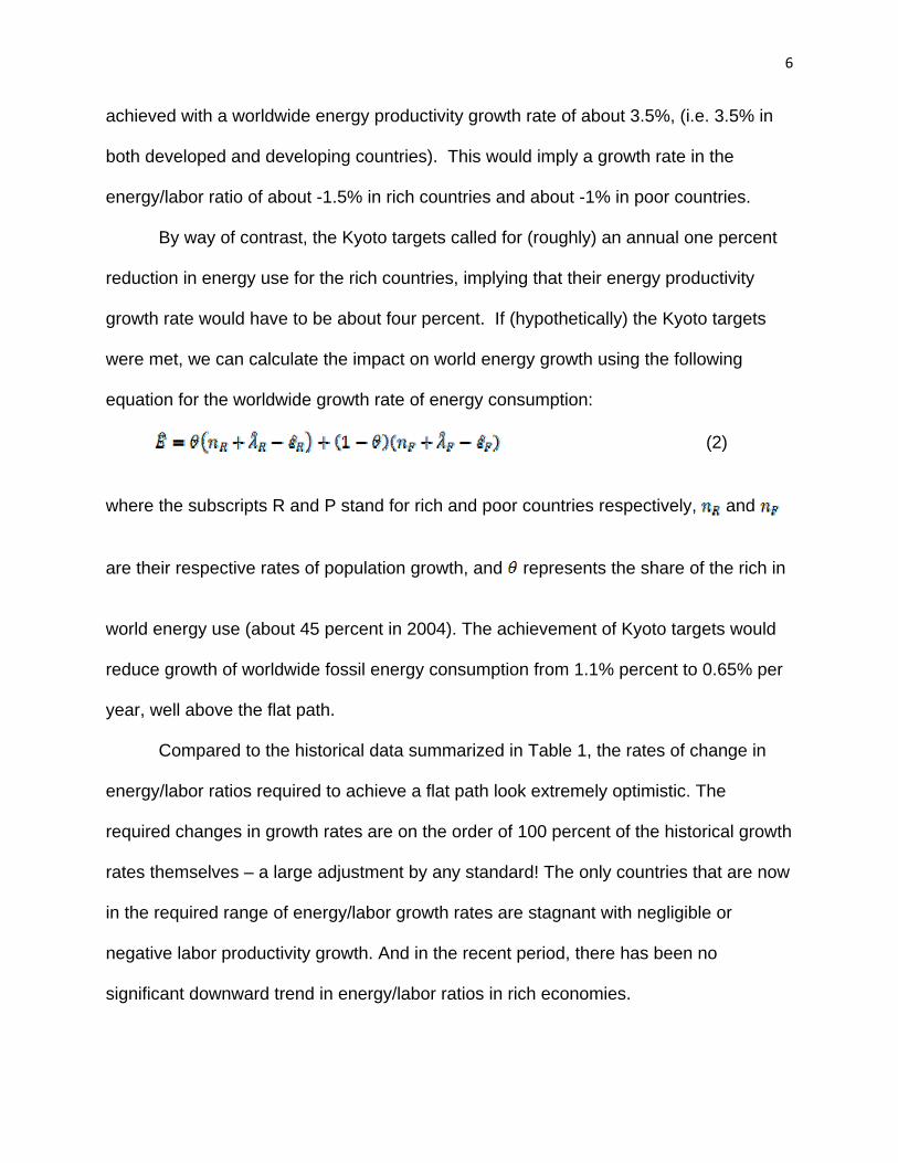
By way of contrast, the Kyoto targets called for (roughly) an annual one percent

reduction in energy use for the rich countries, implying that their energy productivity

growth rate would have to be about four percent. If (hypothetically) the Kyoto targets

were met, we can calculate the impact on world energy growth using the following

equation for the worldwide growth rate of energy consumption:

(2)

where the subscripts R and P stand for rich and poor countries respectively, and

are their respective rates of population growth, and represents the share of the rich in

world energy use (about 45 percent in 2004). The achievement of Kyoto targets would

reduce growth of worldwide fossil energy consumption from 1.1% percent to 0.65% per

year, well above the flat path.

Compared to the historical data summarized in Table 1, the rates of change in

energy/labor ratios required to achieve a flat path look extremely optimistic. The

required changes in growth rates are on the order of 100 percent of the historical growth

rates themselves – a large adjustment by any standard! The only countries that are now

in the required range of energy/labor growth rates are stagnant with negligible or

negative labor productivity growth. And in the recent period, there has been no

significant downward trend in energy/labor ratios in rich economies.

7  

It is also possible that CO2/energy ratios could decline, either due to a

significantly higher proportion of non-carbon energy sources (solar, wind, hydro,

nuclear, etc.) or to the introduction of effective carbon capture and storage technology.

Socolow and Pacala (2006) include these possibilities as potential contributors to a flat

path of carbon emissions. Unless there are truly dramatic changes in these areas,

however, the requirements for changes in energy/labor ratios would not be much less

drastic than those outlined above.

“Medium Term” analysis

To complement these numerical illustrations it makes sense to take an analytical

look at future prospects, over a climatic “medium term,” most appropriately measured in

a time frame of decades.

Let G stand for the atmospheric concentration of CO2, currently on the order of

380 ppmv (parts per million by volume). Concentration per capita (or GHG intensity) can

be expressed as . With labor productivity as we have as

a measure of output per unit of atmospheric carbon.6

Standard analysis of sources of growth suggests that most expansion of real

output per capita is due to increases in labor productivity. To simplify initially we assume

that productivity growth is the only source, so that real global GDP grows at a rate

with n as the rate of worldwide population growth.

8  

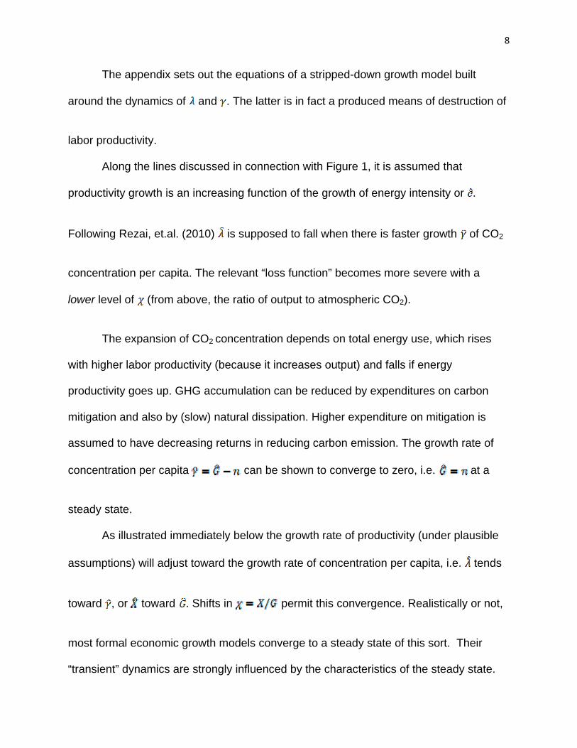
The appendix sets out the equations of a stripped-down growth model built

around the dynamics of and . The latter is in fact a produced means of destruction of

labor productivity.

Along the lines discussed in connection with Figure 1, it is assumed that

productivity growth is an increasing function of the growth of energy intensity or .

Following Rezai, et.al. (2010) is supposed to fall when there is faster growth of CO2

concentration per capita. The relevant “loss function” becomes more severe with a

lower level of (from above, the ratio of output to atmospheric CO2).

The expansion of CO2 concentration depends on total energy use, which rises

with higher labor productivity (because it increases output) and falls if energy

productivity goes up. GHG accumulation can be reduced by expenditures on carbon

mitigation and also by (slow) natural dissipation. Higher expenditure on mitigation is

assumed to have decreasing returns in reducing carbon emission. The growth rate of

concentration per capita can be shown to converge to zero, i.e. at a

steady state.

As illustrated immediately below the growth rate of productivity (under plausible

assumptions) will adjust toward the growth rate of concentration per capita, i.e. tends

toward , or toward . Shifts in permit this convergence. Realistically or not,

most formal economic growth models converge to a steady state of this sort. Their

“transient” dynamics are strongly influenced by the characteristics of the steady state.

9  

In the present case, an additional crucial consideration is that a climate

catastrophe may be inevitable unless the absolute level of atmospheric carbon

becomes constant or decreases. In the world of the model this can only occur if the

population growth rate n becomes zero or negative. Natural dissipation and/or mitigation

might then make total CO2 decrease, along with the level of real GDP.

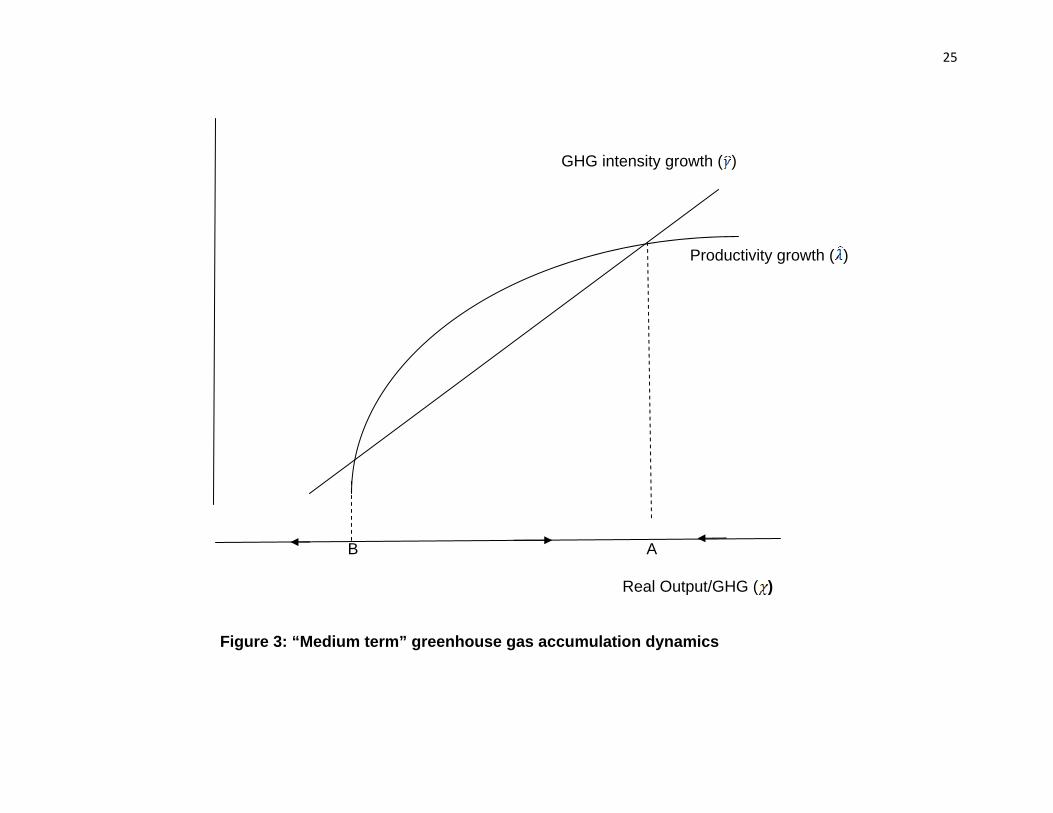
Figure 3 shows how the dynamics works out. Because growth rates of both GHG

intensity ( ) and productivity ( ) depend on it becomes a natural “state variable”

with . The “GHG intensity growth” curve corresponds to equation (A-1) in the

appendix. It shows that is an increasing function of , essentially because more output

creates more emissions.

The “Productivity growth” curve represents equation (A-3). It is concave because

for lower values of (higher values of the ratio ) productivity growth drops off

sharply because of the loss function mentioned above.

Equation (A-4) for shows that the growth model is stable under a plausible

upper bound on the elasticity of the loss function with respect to . As illustrated in

Figure 3, the dynamics resembles that of the Solow-Swan growth model. There is a

stable equilibrium level of at point A, and a potential instability at B due to the

steepness of the loss function. At a full equilibrium, as observed above, it will be true

that .

10  

Figure 3

The model differs from Solow-Swan, however, because the two schedules shift

over time. Growth in GHG intensity decreases when energy productivity rises, and

increases when labor productivity goes up. On balance, the data in Table 1 suggest that

the GHG intensity curve may be shifting upward (largely because of rapid labor

productivity growth in South, Southeast, and East Asia).

To trace through the implications, the first thing to observe is that currently , the

growth rate of CO2 concentration, is on the order of 0.5% per year, well less than the

trend growth of world output. In terms of the model, the current value of must lie

somewhere between points B and A in Figure 3. Because the productivity schedule is

above the GHG intensity schedule for values of in that range, and is rising

over time. An upward shift in the GHG intensity curve would dampen this trend

(worsening global warming), as would a possible downward drift in the Productivity

growth curve.

Policy implications

With these observations as background we can turn the policy implications. The

most immediate one follows from the nature of growth based on produced means of

production or destruction. All dynamic optimization models indicate that means of

production should be produced early in a plan, i.e. first concentrate on producing

machines for Mahalanobis, exports or import substitutes to earn hard currency for

11  

Chenery, or teachers for Lucas. The reason is that the fruits of these early efforts will

support production over a longer time span.

For a produced means of destruction such as atmospheric carbon, the

implication is that mitigation efforts should begin early. They would shift the GHG

schedule downward, causing to rise. The degree of decreasing returns to mitigation

could serve as a guideline about the extent to which the effort should be pursued.

Similar reasoning suggests that slower population growth and more rapid growth

in energy productivity also shift the GHG schedule downward, with a resulting increase

in .

If early mitigation is desirable, how should it be paid for? Output in the model at

hand is fixed by productivity and population in the short run. Saving can be viewed as

increasing physical capital K as a form of infrastructure. New capital goods may also

stimulate productivity directly by embodying better technologies. To capture this

possibility a term such as could be added to equation (A-3) for .

The growth rate of the capital stock as shown in equation (A-5) in the appendix

depends on the saving rate s and a capital utilization rate . Over time utilization

can vary freely over a “reasonable” range of values as K changes with respect to the

level of X coming from productivity growth. Under plausible assumptions u will converge

to a steady state.

12  

Spending on mitigation can be seen as a specific use of a fraction of total

saving sX. The effort becomes less effective at the margin, the higher the value of . At

the same time faster capital stock growth from more saving can raise the productivity

growth rate . In the model’s “short run” of a decade or so an increase in the saving rate

would shift the GHG locus in Figure 3 downward by permitting more spending on

mitigation. It would shift the productivity locus upward. On both counts would

tend to rise because the numerator would go up and the denominator fall.

There has been a lot of discussion in the literature about whether the present

population cohort has to “sacrifice” resources to overcome a GHG “externality.” Foley

(2009) argues convincingly that this question is incorrectly posed. In microeconomic

terms an externality can only be properly defined if the economy is operating efficiently

in all other aspects. The presence of GHG means that the global economy operates

“inside” its production possibility frontier. Moving toward the frontier by increasing

mitigation would create a surplus which could permit both present and future

generations to gain. The former could invest less in conventional capital and use those

resources both to increase consumption and to undertake mitigation. The latter would

benefit from a better allocation involving less conventional capital offset by reductions in

GHG. The optimal growth model reported by Rezai, et. al. (2010) illustrates how Foley’s

arguments apply.

In the present model with the linkage between capital stock growth and

productivity growth in force, a lower saving rate (reversing the thought experiment

13  

described above) would make tend to fall with G increasing and X going down.

However, an increased mitigation effort could move the GHG intensity locus downward

enough to offset these shifts.

Another distributive conflict pivots around how to allocate the cost of mitigation

between rich and poor countries. As in equation (A-2) it is easy to decompose

worldwide GHG expansion into contributions from rich and poor countries. Figure 4 is

an exaggerated hypothetical illustration about how the contributions might change as

overall output increases. The solid lines represent “business as usual” (or BAU). For

“low” (or late 20th century) levels of X most GHG emission comes from rich countries

and the contribution of poor countries is small. For “high” (mid 21st century?) with BAU

the situation changes, as poor countries contribute most of the growth of GHG.

The dashed lines show a mitigation scenario in which the poor country

contribution drops off notably on the assumption that decreasing returns to mitigation

are less onerous in economies which use relatively low levels of energy in production,

often under conditions of low efficiency. Trade-offs about how and where mitigation

should be pursued immediately arise.

On the whole, poor countries import ‘modern’ technologies previously created in

advanced economies. The key policy question in this regard is whether in the near

future rich country energy/labor ratios can be reduced (or energy productivity increased

relative to labor productivity) substantially by technological innovation and social

rearrangements.7 If such innovations work out, then perhaps they can be passed to

developing economies soon enough to enable them to maintain positive per capita

output growth with only slowly increasing or (better) decreasing energy/labor ratios.

14  

If such a growth pattern does not prove to be possible, then the three

contradictory trends mentioned at the outset will inevitably collide. Only 16 percent of

the world’s population now lives in the rich countries which account for 45 percent of

world energy use. Both shares are declining. Unless the advanced economies find the

means to reduce their own energy-labor ratios substantially (and unhistorically) and

pass the techniques along to the rest of the world, the consequences of colliding income

growth, energy use per capita, and global warming trends are unforeseeable but may

well be catastrophic indeed.

Appendix

Using notation already defined in the text, this appendix sets out the equations

behind the growth scenarios depicted in Figures 3-xX. Defining as , the

increase in atmospheric CO2 concentration can be written as

.

Carbon emission rises with energy use according to the coefficient . Let s be the

saving rate from output and the share of saving devoted to mitigation. The function

gauges the effectiveness of mitigation in reducing emission. Presumably it will be

concave. The coefficient reflects the slow natural dissipation of atmospheric CO2.

Dividing both sides of this equation by G gives

.

It follows that

15  

. (A-1)

This equation for the growth rate of CO2 concentration per capita can be restated as

.

This differential equation is stable, so that will converge to a “quasi-steady

state” value

with . Of course, so long as energy and labor productivity levels and are

changing over time will be a moving target for . It will stable when

.

The rapid labor productivity growth rates for well-performing developing regions in Table

1 suggest that they are driving the worldwide level of GHG accumulation up; the

evidence is less clear for the industrialized world.

This line of thought can be pursued one step further. Let be an index for

rich and poor regions, and define as . Then the overall change

in GHG emission becomes

(A-2)

with where the are regional output levels. This sort of decomposition

underlies Figure 4.

16  

The growth of productivity can be described as

in which is a time trend. Faster growth of GHG per capita reduces the growth rate of

output per capita according to the loss function . As decreases (so that the ratio

of GHG to output goes up), the loss becomes more acute. Finally, growth in energy

intensity stimulates productivity growth according to the coefficient (recall the

discussion of Figure 1).

Plugging (A-1) into this equation gives

. (A-3)

and the growth rate of itself becomes

. (A-4)

It is easy to see that the differential equation for will be stable if

, i.e. the absolute value of the elasticity of with respect to is not

“too high”. Again, the quasi-steady state value will be changing over time as a moving

target for .

Figure 3 in the text depicts the dynamics of the system based on (A-1) and (A-3).

A quick extension of the model would be to take into account capital

accumulation. With output determined by labor productivity exclusively, physical capital

17  

is best viewed as providing required infrastructure. New capital goods may also

stimulate productivity directly.

To bring these possibilities into play, let K be the capital stock and be

“utilization,” which is assume to be able to vary freely within some “reasonable” range,

i.e. there are no locally diminishing returns to the use of capital. A simple equation for

capital stock growth then becomes

with s as the saving rate (as above) and the rate of depreciation. Using and

it follows that u satisfies a differential equation

)] . (A-5)

Without going into the details, suppose that in (A-3) is also positively affected

by capital stock growth and thereby the level of u. If the effect is not too strong, (A-5) will

be locally stable with . The time-derivative will also depend negatively on

via (A-3). From (A-4) the productivity linkage means that will depend negatively on

and positively on u. These signs of partial derivatives lead to the configuration of the

phase diagram shown in Figure 5. It could be used to explore long-term developments

in a non-optimizing framework.

Figure 5

18  

Notes

1. New School for Social Research. Ideas from Duncan Foley, Jonathan Harris,

Codrina Rada, and Armon Rezai are gratefully acknowledged.

2. Leibniz proposed the basic concept of energy around 1680 but it did not take

its modern form until the 1840s.

3. The data in this paper were initially presented in Taylor (2009). The country

groups are described in Ocampo, et. al. (2009).

4. One joule is the energy required to lift a small (100 gram) apple one meter

against the earth’s gravity. One terajoule is roughly equivalent to 7700 gallons of

gasoline or 31 tons of coal. Alternatively, one watt equals one joule of energy use per

second. Dividing terajoules per year by the number of seconds in a year shows that an

American worker utilizes 19.3 kilowatts of power to produce his or her contribution to

real GDP. An African uses 300 watts.

5. In any case, switching from the current worldwide mix of fossil fuel energy

sources to using natural gas (the least carbon-intensive source) exclusively would

reduce carbon emissions by only about 15 percent (see Lewis, 2007).

6. The ratio can be interpreted as the “velocity” of the turnover of GHG with

respect to production. In the model being described a fall in (less recycling of GHG)

has an adverse effect on productivity growth.

7. The same observation applies to CO2/energy ratios as well.

19  

REFERENCES

Foley, Duncan K. (2009) “The Economic Fundamentals of Global Warming” in Jonathan

M. Harris and Neva R. Goodwin (eds.) Twenty-First Century Macroeconomics:

Responding to the Climate Challenge, Northhampton MA: Edward Elgar

Lewis, Nathan S. (2007), ‘Powering the Planet’, Engineering and Science, 70 (2): 12–23

Martinez-Alier, Juan and Klaus Schlüpmann (1991), Ecological Economics: Energy,

Environment, and Society, Oxford, UK: Basil Blackwell Publishing.

Mirowski, Phillip (1989), More Heat than Light, Cambridge, UK: Cambridge University

Press.

Ocampo, José Antonio, Codrina Rada, and Lance Taylor (2009) Growth and Policy in

Developing Countries: A Structuralist Approach, New York: Columbia University

Press

Rezai, Armon, Duncan K. Foley, and Lance Taylor (2010) “Global Warming and

Economic Externalities,”

Socolow Robert H., and Stephen W. Pacala (2006), ‘A Plan to Keep Carbon in Check’,

Scientific American, 295 (3): 50–57.

Taylor, Lance (2009) “Energy Productivity, Labor Productivity, and Global Warming” in

Jonathan M. Harris and Neva R. Goodwin (eds.) Twenty-First Century

Macroeconomics: Responding to the Climate Challenge, Northhampton MA:

Edward Elgar

20  

Growth of energy to labor ratio and labor productivity: 1990-2004

-2.0%

-1.0%

0.0%

1.0%

2.0%

3.0%

4.0%

5.0%

6.0%

-2.0% 0.0% 2.0% 4.0% 6.0% 8.0% 10.0%Labor productivity growth

E/L

grow

th

Tigers

Andean

Central Americaand the Caribbean

OECD

Middle East and

N h Af i

Sub Sahara Africa

South Asia

Central and Eastern Europe

South East Asisa

FormerUSSR

China

Semi-industrialized

Growth of energy to labor ratio and labor productivity: 1970-1990

-1.0%

0.0%

1.0%

2.0%

3.0%

4.0%

5.0%

6.0%

7.0%

-2.0% -1.0% 0.0% 1.0% 2.0% 3.0% 4.0% 5.0%Labor productivity growth

E/L

grow

th

Tigers

AndeanCentral Americaand the Caribbean

Semi-industrialized

OECD

Middle East and North Africa

Sub Sahara Africa

South Asia

Central and Eastern Europe

South East Asisa

FormerUSSR

China

 

Figure 1: Growth rates of labor productivity and the energy/labor ratio.

21  

1970-1990

Selected OECD

Central and Eastern Europe

USSR* (1989 end year)

Tigers South East Asia

China South Asia

Semi-Industrialized countries

Central America and the Caribbean

Andean Middle East

SubSahara Africa

Growth Rates Energy Productivity 2.1% 2.4% 1.6% 0.6% -1.3% 1.4% -2.1% -1.0% -0.8% -1.1% -4.9% -3.5% Growth Rates Labor Productivity 1.6% 3.0% 4.0% 4.4% 3.1% 3.9% 1.4% 0.4% -0.2% -1.0% 0.8% 1.6% Growth Rates E/L -0.5% 0.6% 2.3% 3.7% 4.5% 2.5% 3.5% 1.4% 0.6% 0.2% 6.0% 5.3%

E/L beginning year (1970) 0.49

0.21

0.26

0.08

0.01

0.02

0.01

0.09

0.04

0.04

0.05

0.0048

E/L end year (1990) 0.45

0.24

0.40

0.17

0.03

0.04

0.02

0.12

0.05

0.04

0.16

0.0133  

1990-2004

Selected OECD

Central and Eastern Europe

USSR* (beginning year)

Tigers South East Asia

China South Asia

Semi-Industrialized countries

Central America and the Caribbean

Andean Middle East

SubSahara Africa

Growth Rates Energy Productivity 1.9% 3.2% 2.1% 0.4% -1.3% 4.5% 0.8% 0.4% -0.3% 1.0% -0.9% -0.2% Growth Rates Labor Productivity 2.0% 3.2% -0.2% 3.9% 2.6% 8.6% 4.1% 0.8% 1.3% 0.7% 0.6% -0.9% Growth Rates E/L 0.1% 0.0% -0.9% 3.5% 3.9% 3.9% 3.3% 0.4% 1.6% -0.2% 1.5% -0.7%

E/L beginning year (1990) 0.45 0.24 0.41

0.17 0.03

0.04

0.02

0.12

0.05

0.04

0.16

0.01

E/L end year (2004) 0.45 0.24 0.37

0.27 0.05

0.07

0.04

0.12

0.06

0.04

0.19

0.01

Table 1: Growth of energy productivity, labor productivity, and the energy/labor ratio.

Data Sources: World Bank Development Indicators 2005 database; Gronningen Center for Growth and Development

22  

World US UK Sweden France Japan

Total CO2 Emission

(thousands of metric tons)

27,245,758

6,049,435 587,261 53,033 373,693 1,257,963

Total Energy Consumption

(thousands of terajoules)

361,849.00

81,762.00

8,926.00 671.00

5,667.00

17,094.00

Employment

2,836,437 140,702 28,008 4,311 24,963 63,290

Population

6,411,145 293,028 60,271 8,986 60,991 127,480

Energy Consumption/Labor 0.13 0.58 0.32 0.16 0.23 0.27

CO2 Emission/Energy

Consumption 75.3 74.0 65.8 79.0 65.94 74

CO2 Emissions/Population 4.25 20.6 9.7 5.9 6.1 9.9

23  

China India Argentina Brazil Venezuela

South

Africa Kenya

Saudi

Arabia Poland Russia

Total CO2 Emission

(thousands of metric tons) 5,012,377 1,342,962 141,786 331,795 172,623 437,032 10,588 308,393 307,238 1,524,993

Total Energy Consumption

(thousands of terajoules)

51,339

14,890 2,358 4,880 2,295

4,939 119 5,715 3,745 24,355

Employment 752,000 394,612 14,329 71,058 8,855 19,092 15,110 7,675 13,855 66,407

Population 1,295,734 1,065,071 38,984 183,169 24,765 44,448 33,973 25,796 38,580 143,508

Energy Consumption/Labor 0.07 0.04 0.16 0.07 0.26 0.26 0.01 0.74 0.27 0.37

Carbon Emission/Energy

Consumption 97.6 74.0 65.8 79.0 65.94 74 89.0 74.0 73.7 74.7

Carbon Emissions/Population 3.87 1.3 3.6 1.8 7.0 9.8 0.31 12.0 8.0 10.6

Table 2: Carbon dioxide emission and energy consumption in 2004.

Data Sources: Gronningen Center for Growth and Development; 2004 Energy Statistics Yearbook, United Naions; Carbon

Dioxide Information Analysis Center, United States Department of Energy

24  

Required Energy Productivity Growth for Energy Consumption to Remain Constant:1990-2004

0.000

0.010

0.020

0.030

0.040

0.050

0.060

0.070

0.000 0.010 0.020 0.030 0.040 0.050 0.060 0.070 0.080

Energy Productivity Growth OECD

Ener

gy P

rodu

ctiv

ity G

row

th D

evel

opin

g

1990-2004 valuesEnergy growth=1.1%

 

Figure 2: Energy productivity growth rates required to hold overall growth of energy use to zero, 1990-2004

25  

GHG intensity growth ( )

Productivity growth ( )

B A Real Output/GHG ( )

Figure 3: “Medium term” greenhouse gas accumulation dynamics

26  

Contributions to GHG Total emission Poor countries World Real Output (X) Figure 4: Hypothetical contributions to GHG emission

27  

Real Output/GHG ( )

Steady state

Steady state u Real Output/Capital (u) Figure 5: Long term phase diagram for capital utilization and GHG concentration